Hybrid high-order method for singularly perturbed fourth-order problems on curved domains

Abstract

We propose a novel hybrid high-order method (HHO) to approximate singularly perturbed fourth-order PDEs on domains with a possibly curved boundary. The two key ideas in devising the method are the use of a Nitsche-type boundary penalty technique to weakly enforce the boundary conditions and a scaling of the weighting parameter in the stabilization operator that compares the singular perturbation parameter to the square of the local mesh size. With these ideas in hand, we derive stability and optimal error estimates over the whole range of values for the singular perturbation parameter, including the zero value for which a second-order elliptic problem is recovered. Numerical experiments illustrate the theoretical analysis.

1 Introduction

Fourth-order singular perturbed PDEs are used in the modeling of various physical phenomena, such as thin plate elasticity, micro-electromechanical systems, and phase separation to mention a few examples. In the present work, we consider the following model problem: Find $u:\Omega\to\mathbb{R}$ such that

$$\left\{\begin{aligned} \varepsilon\Delta^{2}u-\Delta u&=f&\qquad&\text{in $\Omega$},\\ u&=g_{\rm D}&\qquad&\text{on $\partial\Omega$},\\ \varepsilon{\bf n}_{\Omega}{\cdot}\nabla u&=\varepsilon g_{\rm N}&\qquad&\text{on $\partial\Omega$},\end{aligned}\right.$$ (1)

where $\Omega$ is a open bounded Lipschitz domain in $\mathbb{R}^{d}$, $d=2,3$, with boundary $\partial\Omega$ and unit outward normal ${\bf n}_{\Omega}$. The problem data are the forcing term $f:\Omega\to\mathbb{R}$ and the Dirichlet and Neumann data $g_{\rm D},g_{\rm N}:\partial\Omega\to\mathbb{R}$. The assumptions on the data are specified below. The use of other boundary conditions in (1) is currently under study. Moreover, the perturbation parameter $\varepsilon$ is a nonnegative real number, i.e., we only assume that $\varepsilon\geq 0$, and we are especially interested in the singularly perturbed regime where $\varepsilon\ll\ell_{\Omega}^{2}$, where $\ell_{\Omega}$ is some suitable length scale associated with $\Omega$, e.g., its diameter ($\ell_{\Omega}=1$ if the problem is written in nondimensional form). Notice that the Neumann boundary condition is scaled by $\varepsilon$ so that the model problem (1) becomes the Poisson problem with Dirichlet boundary condition when $\varepsilon=0$. Another feature of interest here is that the domain $\Omega$ can have a curved boundary.

The purpose of this work is to design and analyze a hybrid high-order (HHO) method to approximate the model problem (1). The key feature of the proposed method is its ability to handle in a robust way the whole scale for the singular perturbation parameter $\varepsilon\in[0,\ell_{\Omega}^{2}]$ (notice that the value $\varepsilon=0$ is allowed). HHO methods were introduced in [14] for linear diffusion and in [13] for locking-free linear elasticity. In such methods, discrete unknowns are attached to the mesh cells and to the mesh faces. The two key ingredients to devise HHO methods are a local reconstruction operator and a local stabilization operator in each mesh cell. HHO methods offer various attractive features, such as the support of polytopal meshes, optimal error estimates, local conservation properties, and computational efficiency due to compact stencils and local elimination of the cell unknowns by static condensation. As a result, these methods have been developed extensively over the past few years and now cover a broad range of applications; we refer the reader to the two recent monographs [12, 8] for an overview. As shown in [9], HHO methods can be embedded into the broad framework of hybridizable discontinuous Galerkin (HDG) methods, and they can be bridged to nonconforming virtual element methods (ncVEM). Moreover, HHO methods are closely related to weak Galerkin (WG) methods. Indeed, the reconstruction operator in the HHO method corresponds to the weak gradient (or any other differential operator) in WG methods, so that the only relevant difference between HHO and WG methods lies in the choice of the discrete unknowns and the design of the stabilization operator.

Various HHO methods for the biharmonic operator were devised and analyzed recently in [15], including a comparison with existing WG methods for the biharmonic operator. We also refer the reader to [1] for the first HHO method for the biharmonic operator in primal form. In [15], two HHO methods were proposed (called HHO-A and HHO-B). Both methods use cell unknowns to approximate the solution in each mesh cell, face unknowns to approximate its trace on the mesh faces, and face unknowns to approximate its normal derivatives on the mesh faces. In both methods, the cell unknowns are polynomials of degree $(k+2)$ and the face unknowns for the normal derivative are polynomials of degree $k$, with $k\geq 0$. HHO-A is restricted to two space dimensions and uses polynomials of degree $(k+1)$ for the face unknowns related to the trace, whereas HHO-B supports any space dimension but uses polynomials of degree $(k+2)$ for these face unknowns. Moreover, the HHO-A method was combined in [15] with a Nitsche-type boundary penalty technique, originally introduced in [7] to weakly enforce Dirichlet conditions in HHO methods for second-order PDEs and further developed in [4, 3] to handle unfitted meshes in problems with a curved interface or boundary. In particular, one of the advances in [3] is that the weighting parameter in the boundary penalty term does not need to be large enough, but only positive.

In the present work, our starting point is the HHO-B method from [15]. Consistently with the paradigm considered for singularly perturbed second-order elliptic PDEs, the boundary conditions in (1) are weakly enforced by means of a Nitsche-type boundary penalty technique. This is the first key idea to capture possible boundary layers and to achieve robustness for the singularly perturbed fourth-order elliptic problem. The second key idea to achieve robustness is to revisit the weighting of the stabilization operator in the HHO-B method by including a scaling factor that compares the singular perturbation parameter $\varepsilon$ with the square of the (local) mesh size. With these two ideas in hand, we can devise a novel HHO method that remains uniformly stable over the full range $\varepsilon\in[0,\ell_{\Omega}^{2}]$ and that delivers optimally decaying error estimates, both in the case $\varepsilon\approx\ell_{\Omega}^{2}$ (representative of a fourth-order PDE) and in the case $\varepsilon\ll\ell_{\Omega}^{2}$ and even $\varepsilon=0$ (representative of a second-order PDE). In a nutshell (see Theorem 4.5 for a more precise statement and the remarks below for a discussion), the error estimate takes the general form $\varepsilon^{\frac{1}{2}}\|\nabla^{2}e\|_{\Omega}+\|\nabla e\|_{\Omega}\leq C(\varepsilon^{\frac{1}{2}}h^{k+1}+h^{k+2})$, where $e$ represents the approximation error, $h$ the mesh size, and the constant $C$ depends on the regularity of the exact solution, the shape-regularity of the underlying meshes, and the polynomial degree $k\geq 0$. An additional benefit of using the Nitsche-type boundary penalty technique is the seamless support of domains with a curved boundary, in the wake of the ideas developed in [4, 3] for second-order PDEs.

Let us briefly put our contribution in perspective with the literature on singularly perturbed fourth-order PDEs. Consistently with the present approach, we focus on discretization methods that hinge on the primal form of the PDE and thus lead, at the algebraic level, to a symmetric positive definite linear system. To the best of our knowledge, the present method appears to be the first in the literature that, at the same time, supports polytopal meshes and offers a robust behavior over the full range of values for the singular perturbation parameter $\varepsilon$. On the one hand, robust approximation methods developed on specific meshes (composed, e.g., of simplices or cuboids) include $C^{0}$-interior penalty discontinuous Galerkin (IPDG) methods [2] and methods based on the modified Morley element [21, 26, 25, 19, 24], for which a weak enforcement of the boundary conditions using Nitsche-type techniques was considered more recently in [27, 20]. On the other hand, discretization methods for singularly perturbed fourth-order operators on polytopal meshes include the WG method from [10] and the $C^{0}$-ncVEM from [29]. Both methods, however, do not support the limit with $\varepsilon=0$ and in this case lead, at the algebraic level, to a singular linear system. More precisely, in this limit, the sub-blocks coupling the face unknowns discretizing the gradient (or the normal gradient) on the faces either to the other unknowns or to themselves all vanish. Thus, to recover a nonsingular linear system when $\varepsilon=0$, one needs to manually remove these gradient face unknowns, but unfortunately this fix cannot be applied when $\varepsilon\ll 1$, leading to serious conditioning issues in this case. This situation is instead avoided by the present method: by including a mesh-dependent cutoff in the stabilization coefficient coupling the gradient face unknowns to the other unknowns, the linear system at the limit $\varepsilon=0$ remains nonsingular without any need to remove manually some unknowns.

The rest of this work is organized as follows. We present the weak formulation of the model problem together with the discrete setting in Section 2. In Section 3, we introduce the present HHO method. In Section 4, we present our main results on the stability and error analysis of the HHO method. Numerical results are discussed in Section 5. Finally, the proofs of our main results are collected in Section 6.

2 Weak formulation and discrete setting

In this section, we present the weak formulation of the model problem (1) together with the discrete setting.

2.1 Weak formulation

We use standard notation for the Lebesgue and Sobolev spaces. In particular, when considering fractional-order Sobolev spaces, we use the Sobolev–Slobodeckij seminorm based on the double integral. For an open, bounded, Lipschitz set $S$ in $\mathbb{R}^{d}$, $d\in\{1,2,3\}$, with a piecewise smooth boundary, we denote by $(v,w)_{S}$ the $L^{2}(S)$-inner product, and we employ the same notation when $v$ and $w$ are vector- or matrix-valued fields. We denote by $\nabla w$ the (weak) gradient of $w$ and by $\nabla^{2}w$ its (weak) Hessian. It is convenient to consider the following inner product and corresponding seminorm on $\varepsilon H^{2}(S)+H^{1}(S)$ (this is just a shortcut notation for $H^{2}(S)$ if $\varepsilon>0$ and $H^{1}(S)$ if $\varepsilon=0$):

$$(\nabla v,\nabla w)_{S,\varepsilon}:=\varepsilon(\nabla^{2}v,\nabla^{2}w)_{S}+(\nabla v,\nabla w)_{S},\qquad\|\nabla v\|_{S,\varepsilon}^{2}:=(\nabla v,\nabla v)_{S,\varepsilon}.$$ (2)

Let ${\bf n}_{S}$ be the unit outward normal vector on the boundary $\partial S$ of $S$. Assuming that the functions $v$ and $w$ are smooth enough, we have the following integration by parts formula:

$$\varepsilon(\Delta^{2}v,w)_{S}-(\Delta v,w)_{S}={} (\nabla v,\nabla w)_{S,\varepsilon}+\varepsilon\big{(}(\nabla\Delta v,{\bf n}_{S}w)_{\partial S}-(\nabla^{2}v{\bf n}_{S},\nabla w)_{\partial S}\big{)}-(\nabla v,{\bf n}_{S}w)_{\partial S}.$$ (3)

To alleviate the notation, it is implicitly understood that within integrals over $\partial S$, $\partial_{n}$ denotes the normal derivative on $\partial S$ along ${\bf n}_{S}$. Moreover, $\partial_{t}$ denotes the ($\mathbb{R}^{d-1}$-valued) tangential derivative on $\partial S$. We also denote by $\partial_{nn}v$ the (scalar-valued) normal-normal second-order derivative and by $\partial_{nt}v$ the ($\mathbb{R}^{d-1}$-valued) normal-tangential second-order derivative. The integration by parts formula (3) can then be rewritten as

$$\varepsilon(\Delta^{2}v,w)_{S}-(\Delta v,w)_{S}={} (\nabla v,\nabla w)_{S,\varepsilon}+\varepsilon\big{(}(\partial_{n}\Delta v,w)_{\partial S}-(\partial_{nn}v,\partial_{n}w)_{\partial S}-(\partial_{nt}v,\partial_{t}w)_{\partial S}\big{)}-(\partial_{n}v,w)_{\partial S}.$$ (4)

Let us consider the Hilbert spaces $V:=\varepsilon H^{2}(\Omega)+H^{1}(\Omega)$ and $V_{0}:=\varepsilon H^{2}_{0}(\Omega)+H^{1}_{0}(\Omega)$ equipped with the inner product $(\nabla v,\nabla w)_{\Omega,\varepsilon}$. Assume that the source term in (1) satisfies $f\in L^{2}(\Omega)$ and that the boundary data are such that there is $u_{g}\in V$ such that $u_{g}=g_{\rm D}$ and $\varepsilon{\bf n}{\cdot}\nabla u_{g}=\varepsilon g_{\rm N}$ on $\partial\Omega$. Using the above integration by parts formula, the following weak formulation for (1) is derived: Find $u\in u_{g}+V_{0}$ such that

$$(\nabla u,\nabla w)_{\Omega,\varepsilon}=(f,w)_{\Omega},\qquad\forall w\in V_{0}.$$ (5)

The Lax–Milgram lemma readily shows that this problem is well-posed.

2.2 Polytopal and curved meshes

In this work, we assume that $\partial\Omega$ can be covered by a finite number of closed $C^{2}$ manifolds with nonoverlapping interior, and we write $\partial\Omega=\bigcup_{m\in\{1,\ldots,N_{\partial}\}}S_{m}$. Let $\{\mathcal{T}_{h}\}_{h>0}$ be a mesh family such that each mesh $\mathcal{T}_{h}$ covers $\Omega$ exactly. A generic mesh cell is denoted by $K\in\mathcal{T}_{h}$, its diameter by $h_{K}$, and its unit outward normal by ${\bf n}_{K}$. We define the following mesh-dependent parameter for measuring locally the dominant operator in the PDE: For all $K\in\mathcal{T}_{h}$,

$$\sigma_{K}:=\max\{1,\varepsilon h^{-2}_{K}\}.$$ (6)

We partition the boundary $\partial K$ of any mesh cell $K\in\mathcal{T}_{h}$ by means of the two subsets $\partial K^{\mathrm{i}}:=\overline{\partial K\cap\Omega}$ and $\partial K^{\mathrm{b}}:=\partial K\cap\partial\Omega$. Similarly, we partition the mesh as $\mathcal{T}_{h}=\mathcal{T}_{h}^{\mathrm{i}}\cup\mathcal{T}_{h}^{\mathrm{b}}$, where $\mathcal{T}_{h}^{\mathrm{b}}$ is the collection of all the mesh cells $K$ such that $\partial K^{\mathrm{b}}$ has positive measure. The mesh faces are collected in the set $\mathcal{F}_{h}$, which is split as $\mathcal{F}_{h}=\mathcal{F}_{h}^{\mathrm{i}}\cup\mathcal{F}_{h}^{\mathrm{b}}$, where $\mathcal{F}_{h}^{\mathrm{i}}$ is the collection of the interior faces (shared by two distinct mesh cells) and $\mathcal{F}_{h}^{\mathrm{b}}$ the collection of the boundary faces. For all $F\in\mathcal{F}_{h}$, we orient $F$ by means of the fixed unit normal vector ${\bf n}_{F}$ whose direction is arbitrary for all $F\in\mathcal{F}_{h}^{\mathrm{i}}$ and ${\bf n}_{F}:={\bf n}_{\Omega}$ for all $F\in\mathcal{F}_{h}^{\mathrm{b}}$. For any mesh cell $K\in\mathcal{T}_{h}$, the mesh faces composing its boundary $\partial K$ are collected in the set $\mathcal{F}_{\partial K}$, which is partitioned as $\mathcal{F}_{\partial K}=\mathcal{F}_{\partial K^{\mathrm{i}}}\cup\mathcal{F}_{\partial K^{\mathrm{b}}}$ with obvious notation. To avoid distracting technicalities, we assume that each mesh $\mathcal{T}_{h}$ is compatible with the decomposition $\partial\Omega=\bigcup_{m\in\{1,\ldots,N_{\partial}\}}S_{m}$, so that for all $K\in\mathcal{T}_{h}^{\mathrm{b}}$, each face $F\in\mathcal{F}_{\partial K^{\mathrm{b}}}$ is a closed $C^{2}$ manifold.

In this work, we consider mesh sequences satisfying the following mesh shape-regularity assumption.

Assumption 2.1 (Mesh shape-regularity)

(i) Any interior mesh cell $K\in\mathcal{T}_{h}^{\mathrm{i}}$ is a polytope with planar faces, and the sequence of interior meshes $\{\mathcal{T}_{h}^{\mathrm{i}}\}_{h>0}$ is shape-regular in the sense of [13, Definition 1]. (ii) For any boundary mesh cell $K\in\mathcal{T}_{h}^{\mathrm{b}}$, all the faces in $\mathcal{F}_{\partial K^{\mathrm{i}}}$ are planar with diameter uniformly equivalent to $h_{K}$, and all the faces in $\mathcal{F}_{\partial K^{\mathrm{b}}}$ are subsets of $\partial\Omega$ which are closed $C^{2}$ manifolds. Moreover, for each $F\in\mathcal{F}_{\partial K^{\mathrm{b}}}$, $K$ can be decomposed into a finite union of nonoverlapping subsets, $\{K_{F,m}\}_{m\in\{1,\ldots,n_{K,F}\}}$, so that each $K_{F,m}$ is star-shaped with respect to an interior ball of radius uniformly equivalent to $h_{K}$; see Figure 1 for an illustration with $n_{K,F}=1$. (Notice that the star-shapedness assumption implies that $n_{K,F}$ is uniformly bounded.)

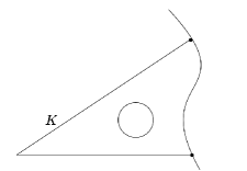
Figure 1: Example of a boundary mesh cell with a curved boundary face and which is star-shaped with respect an interior ball; • denotes a mesh vertex at the boundary.

Remark 2.2 (Mesh assumptions)

The above assumptions on the mesh sequence are fairly general. Let us briefly discuss some of the most significant ones. (i) The assumption that each mesh $\mathcal{T}_{h}$ covers $\Omega$ exactly is reasonable in the present context where boundary conditions are enforced by means of a Nitsche-like penalty method. In particular, all the integrals in the mesh cells and their faces are performed in the physical space without invoking a geometric mapping that can introduce some error due to the approximation of the geometry. To avoid distracting technicalities, we do not consider quadrature errors in our error analysis. (ii) The assumption that the interior faces of the mesh are planar is important in the present setting of HHO methods which use polynomial functions as discrete unknowns attached to these interior faces. Notice though that the use of a Nitsche-like penalty method allows us to avoid introducing discrete unknowns on the boundary faces; thus, such faces do not need to be planar. (iii) The star-shapedness assumption on the mesh boundary cells is introduced to invoke a Poincaré-type inequality in such cells (and, more generally, polynomial approximation properties; see Lemma 2.5 below). An alternative is to invoke an extension operator when asserting polynomial approximation properties, as, for instance, in [4]. In this case, only the multiplicative trace inequality (see Lemma 2.4 below) requires a star-shapedness assumption for the mesh boundary cells, but for this latter result to hold, star-shapedness with respect to an interior point for each $K_{F,m}$ is a sufficient assumption [6, Lemma 32] (and in this setting, the number $n_{K,F}$ does no longer need to be uniformly bounded).

2.3 Analysis tools

Let us briefly review the main analysis tools used in this work. We simply state the results and refer the reader to Remark 2.6 for some comments on the proofs. In what follows, we always consider a shape-regular mesh sequence satisfying Assumption 2.1. Moreover, in various bounds, we use the symbol $C$ to denote any positive generic constant (its value can change at each occurrence) that is independent of $h>0$, the considered mesh cell $K\in\mathcal{T}_{h}$, and the considered function in the inequality. The value of $C$ can depend on the parameters quantifying the shape-regularity of the mesh sequence and the polynomial degree (whenever relevant).

Lemma 2.3 (Discrete inverse inequalities)

Let $l\geq 0$ be the polynomial degree. There is $C$ (depending on $l$) such that for all $h>0$, all $K\in\mathcal{T}_{h}$, and all $v_{h}\in\mathbb{P}^{l}(K)$,

$$\|{v}_{h}\|_{\partial K} \leq Ch_{K}^{-\frac{1}{2}}\|{v}_{h}\|_{K},$$ (7)

$$\|\nabla{v}_{h}\|_{K} \leq Ch_{K}^{-1}\|{v}_{h}\|_{K},$$ (8)

$$\|\partial_{t}{v}_{h}\|_{F} \leq Ch_{K}^{-1}\|{v}_{h}\|_{F},\quad\forall F\in\mathcal{F}_{\partial K^{\mathrm{i}}}.$$ (9)

Lemma 2.4 (Multiplicative trace inequality)

There is $C$ such that for all $h>0$, all $K\in\mathcal{T}_{h}$, and all $v\in H^{1}(K)$,

$$\|{v}\|_{\partial K}\leq C\big{(}h_{K}^{-\frac{1}{2}}\|{v}\|_{K}+h_{K}^{\frac{1}{2}}|v|_{H^{1}(K)}\big{)}.$$ (10)

Lemma 2.5 (Polynomial approximation)

Let $l\geq 0$ be the polynomial degree. There is $C$ (depending on $l$) such that for all $r\in[0,l+1]$, all $m\in\{0,\ldots,\lfloor r\rfloor\}$, all $h>0$, all $K\in\mathcal{T}_{h}$, and all $v\in H^{r}(K)$,

$$|{v}-\Pi^{l}_{K}(v)|_{H^{m}(K)}\leq Ch^{r-m}_{K}|{v}|_{H^{r}(K)},$$ (11)

where $\Pi_{K}^{l}$ denotes the $L^{2}$-orthogonal projection onto $\mathbb{P}^{l}(K)$.

Let us briefly highlight some useful consequences of the above results. First, (11) includes the following Poincaré-like inequalities (take, respectively, $l=0$, $r=1$, and $l=1$, $r=2$, $m\in\{0,1\}$ in (11)): For all $K\in\mathcal{T}_{h}$,

$$\|v-\Pi_{K}^{0}(v)\|_{K}\leq Ch_{K}\|\nabla v\|_{K}, \forall v\in H^{1}(K),$$ (12)

$$\|v-\Pi_{K}^{1}(v)\|_{K}+h_{K}\|\nabla(v-\Pi_{K}^{1}(v))\|_{K}\leq Ch_{K}^{2}\|\nabla^{2}v\|_{K}, \forall v\in H^{2}(K).$$ (13)

The following consequences of (12)-(13) combined with the multiplicative trace inequality (10) will be useful in our analysis: Letting $k\geq 0$ be the polynomial degree, we have for all $v\in H^{2}(K)$,

$$h_{K}^{-\frac{1}{2}}\|v-\Pi_{K}^{k+2}(v)\|_{\partial K}\leq C\|\nabla(v-\Pi_{K}^{k+2}(v))\|_{K},$$ (14)

$${h_{K}^{-\frac{3}{2}}}\|v-\Pi_{K}^{k+2}(v)\|_{\partial K}+h_{K}^{-\frac{1}{2}}\|\nabla(v-\Pi_{K}^{k+2}(v))\|_{\partial K}\leq C\|\nabla^{2}(v-\Pi_{K}^{k+2}(v))\|_{K}.$$ (15)

Recalling that $\sigma_{K}$ is defined in (6) and the norm $\|{\cdot}\|_{K,\varepsilon}$ in (2) (with $S:=K$), we have for all $v\in H^{2}(K)$,

$$\sigma_{K}^{\frac{1}{2}}h_{K}^{-\frac{1}{2}}\|v-\Pi_{K}^{k+2}(v)\|_{\partial K}\leq C\|\nabla(v-\Pi_{K}^{k+2}(v))\|_{K,\varepsilon}.$$ (16)

Remark 2.6 (Proofs)

Let us briefly comment on the proofs of the above lemmas. Concerning Lemma 2.3 and Lemma 2.4, the proof on mesh cells having flat faces can be found, e.g., in [11, Sec. 1.4.3]. On mesh cells having a curved face, these results are established, e.g., in [4, 28] assuming that the curved face is a $C^{2}$ manifold. More recently, these results were extended in [5] with fully explicit constants to $C^{1}$ manifolds (and sometimes even Lipschitz) and some mild additional geometric assumptions.

Concerning Lemma 2.5, the key step is to establish the Poincaré inequality (12) since (11) can then be derived by using recursively the Poincaré inequality. On the interior mesh cells, which can be decomposed as a finite union of (convex) subsimplices, this latter inequality is established by proceeding as in [23, 16]. On the boundary mesh cells, which can have a curved face, one invokes the star-shapedness assumption with respect to a ball. We refer the reader to [30] for the derivation of this inequality with an explicitly determined constant under such an assumption.

3 HHO discretization

In this section, we first introduce the local ingredients to formulate the HHO discretization in each mesh cell and then we derive the global discrete problem.

3.1 Local unknowns, reconstruction, and stabilization

Let $k\geq 0$ be the polynomial degree. For all $K\in\mathcal{T}_{h}$, the local HHO space is

$$\widehat{V}_{K}^{k}:=\mathbb{P}^{k+2}(K)\times\mathbb{P}^{k+2}(\mathcal{F}_{\partial K^{\mathrm{i}}})\times\mathbb{P}^{k}(\mathcal{F}_{\partial K^{\mathrm{i}}}),$$ (17)

where $\mathbb{P}^{l}(\mathcal{F}_{\partial K^{\mathrm{i}}}):=\times_{F\in\mathcal{F}_{\partial K^{\mathrm{i}}}}\mathbb{P}^{l}(F)$ for all $l\geq 0$. Notice that we do not introduce any discrete unknowns on the faces of $K$ that lie on the boundary. A generic element in $\widehat{V}_{K}^{k}$ is denoted $\widehat{v}_{K}=(v_{K},v_{\partial K},\gamma_{\partial K})$ with $v_{K}\in\mathbb{P}^{k+2}(K)$, $v_{\partial K}\in\mathbb{P}^{k+2}(\partial K^{\mathrm{i}})$, and $\gamma_{\partial K}\in\mathbb{P}^{k}(\partial K^{\mathrm{i}})$. The first component of $\widehat{v}_{K}$ aims at representing the solution inside the mesh cell, the second its trace on the interior part of the cell boundary, and the third its normal derivative on the interior part of the cell boundary (along the direction of the outward normal ${\bf n}_{K}$).

We define the local reconstruction operator $R_{K}^{\mathrm{i}}:\widehat{V}_{K}^{k}\rightarrow\mathbb{P}^{k+2}(K)$ such that, for all $\widehat{v}_{K}\in\widehat{V}_{K}^{k}$ with $\widehat{v}_{K}:=(v_{K},v_{\partial K},\gamma_{\partial K})$, the polynomial $R_{K}^{\mathrm{i}}(\widehat{v}_{K})\in\mathbb{P}^{k+2}(K)$ is uniquely defined by solving the following problem with test functions $w\in\mathbb{P}^{k+2}(K)^{\perp}:=\{w\in\mathbb{P}^{k+2}(K)\;|\;(w,1)_{K}=0\}$:

$$(\nabla R_{K}^{\mathrm{i}}(\widehat{v}_{K}),\nabla w)_{K,\varepsilon}={} (v_{K},\varepsilon\Delta^{2}w)_{K}-(v_{K},\Delta w)_{K}+(v_{\partial K},\partial_{n}w)_{\partial K^{\mathrm{i}}}$$

$$-\varepsilon\Big{\{}(v_{\partial K},\partial_{n}\Delta w)_{\partial K^{\mathrm{i}}}-(\gamma_{\partial K},\partial_{nn}w)_{\partial K^{\mathrm{i}}}-(\partial_{t}v_{\partial K},\partial_{nt}w)_{\partial K^{\mathrm{i}}}\Big{\}},$$ (18)

together with the condition $(R_{K}^{\mathrm{i}}(\widehat{v}_{K}),1)_{K}=(v_{K},1)_{K}$. Integration by parts shows that (18) is equivalent to

$$(\nabla R_{K}^{\mathrm{i}}(\widehat{v}_{K}),\nabla w)_{K,\varepsilon}={} (\nabla{v}_{K},\nabla w)_{K,\varepsilon}-(v_{K}-v_{\partial K},\partial_{n}w)_{\partial K^{\mathrm{i}}}-(v_{K},\partial_{n}w)_{\partial K^{\mathrm{b}}}$$

$$+\varepsilon\Big{\{}(v_{K}-v_{\partial K},\partial_{n}\Delta w)_{\partial K^{\mathrm{i}}}-(\partial_{n}v_{K}-\gamma_{\partial K},\partial_{nn}w)_{\partial K^{\mathrm{i}}}-(\partial_{t}(v_{K}-v_{\partial K}),\partial_{nt}w)_{\partial K^{\mathrm{i}}}$$

$$+(v_{K},\partial_{n}\Delta w)_{\partial K^{\mathrm{b}}}-(\nabla v_{K},\nabla\partial_{n}w)_{\partial K^{\mathrm{b}}}\Big{\}}.$$ (19)

Notice that $(\nabla v_{K},\nabla\partial_{n}w)_{\partial K^{\mathrm{b}}}=(\partial_{n}v_{K},\partial_{nn}w)_{\partial K^{\mathrm{b}}}+(\partial_{t}v_{K},\partial_{nt}w)_{\partial K^{\mathrm{b}}}$.

The local stabilization bilinear form is composed of a contribution on $\partial K^{\mathrm{i}}$ and one on $\partial K^{\mathrm{b}}$. These two contributions are defined such that, for all $(\widehat{v}_{K},\widehat{w}_{K})\in\widehat{V}_{K}^{k}\times\widehat{V}_{K}^{k}$, with $\widehat{v}_{K}:=(v_{K},v_{\partial K},\gamma_{\partial K})$ and $\widehat{w}_{K}:=(w_{K},w_{\partial K},\chi_{\partial K})$,

$$S^{\mathrm{i}}_{\partial K}(\widehat{v}_{K},\widehat{w}_{K}):={} \sigma_{K}h_{K}^{-1}\big{(}v_{\partial K}-v_{K},w_{\partial K}-{w}_{K}\big{)}_{\partial K^{\mathrm{i}}}+\sigma_{K}h_{K}\big{(}\Pi^{k}_{\partial K^{\mathrm{i}}}(\gamma_{\partial K}-\partial_{n}{v}_{K}),\chi_{\partial K}-\partial_{n}{w}_{K}\big{)}_{\partial K^{\mathrm{i}}},$$ (20)

and

$$S^{\mathrm{b}}_{\partial K}(v_{K},w_{K}):={} \sigma_{K}h_{K}^{-1}\big{(}v_{K},{w}_{K}\big{)}_{\partial K^{\mathrm{b}}}+\varepsilon h_{K}^{-1}\big{(}\nabla{v}_{K},\nabla{w}_{K}\big{)}_{\partial K^{\mathrm{b}}},$$ (21)

where $\Pi^{k}_{\partial K^{\mathrm{i}}}$ denotes the $L^{2}$-orthogonal projection onto the broken polynomial space $\mathbb{P}^{k}(\mathcal{F}_{\partial K^{\mathrm{i}}})$.

Finally, we define the local bilinear form $\widehat{a}_{K}$ on $\widehat{V}_{K}^{k}\times\widehat{V}_{K}^{k}$ such that

$$\widehat{a}_{K}(\widehat{v}_{K},\widehat{w}_{K}):=(\nabla R_{K}^{\mathrm{i}}(\widehat{v}_{K}),\nabla R_{K}^{\mathrm{i}}(\widehat{w}_{K}))_{K,\varepsilon}+S^{\mathrm{i}}_{\partial K}(\widehat{v}_{K},\widehat{w}_{K})+S^{\mathrm{b}}_{\partial K}(v_{K},w_{K}).$$ (22)

Remark 3.1 (Reconstruction)

There are two differences with the reconstruction operator introduced in [15] for the biharmonic problem. First, as expected, the terms related to the second-order operator are added, whereas the terms related to the fourth-order operator are scaled by $\varepsilon$. The second difference is more subtle and is inspired from the ideas in [3] for the second-order operator and extended here to the fourth-order operator as well. It consists in discarding the integrals over $\partial K^{\mathrm{b}}$ and only keeping the integrals over $\partial K^{\mathrm{i}}$ for all the boundary terms on the right-hand side of (18). Following the ideas in [7], it is also possible to keep the boundary terms and to use the trace of the cell unknown $v_{K}$ and its normal derivative on $\partial K^{\mathrm{b}}$ to evaluate them. The disadvantage of this latter approach is that the Nitsche-type boundary penalty terms need then to be weighted by a coefficient that is large enough, whereas the weighting coefficient needs only to be positive in the present setting.

Remark 3.2 (Stabilization)

The interior stabilization bilinear form $S^{\mathrm{i}}_{\partial K}$ is inspired from [15] and is weighted here by the local coefficient $\sigma_{K}$ defined in (6) to cover both regimes of interest (dominant Laplacian and dominant bi-Laplacian). Moreover, the boundary stabilization bilinear form $S^{\mathrm{b}}_{\partial K}$ is associated with the Nitsche-type boundary penalty. We emphasize that this latter bilinear form does not need to be weighted by a coefficient which is large enough.

3.2 The global discrete problem

Recall that $k\geq 0$ is the polynomial degree and that the local HHO space $\widehat{V}_{K}^{k}$ is defined in (17) for all $K\in\mathcal{T}_{h}$. The global HHO space is defined as

$$\widehat{V}_{h}^{k}:=\mathbb{P}^{k+2}(\mathcal{T}_{h})\times\mathbb{P}^{k+2}(\mathcal{F}_{h}^{\mathrm{i}})\times\mathbb{P}^{k}(\mathcal{F}_{h}^{\mathrm{i}}).$$ (23)

A generic element in $\widehat{V}_{h}^{k}$ is denoted $\widehat{v}_{h}:=(v_{\mathcal{T}_{h}},v_{\mathcal{F}_{h}^{\mathrm{i}}},\gamma_{\mathcal{F}_{h}^{\mathrm{i}}})$ with $v_{\mathcal{T}_{h}}:=(v_{K})_{K\in\mathcal{T}_{h}}$, $v_{\mathcal{F}_{h}^{\mathrm{i}}}:=(v_{F})_{F\in\mathcal{F}_{h}^{\mathrm{i}}}$, and $\gamma_{\mathcal{F}_{h}^{\mathrm{i}}}:=(\gamma_{F})_{F\in\mathcal{F}_{h}^{\mathrm{i}}}$, where $\gamma_{F}$ is meant to approximate the normal derivative in the direction of the unit normal vector ${\bf n}_{F}$ orienting $F$. For all $K\in\mathcal{T}_{h}$, the local components of $\widehat{v}_{h}$ are collected in the triple $\widehat{v}_{K}:=(v_{K},v_{\partial K},\gamma_{\partial K})\in\widehat{V}_{K}^{k}$ with $v_{\partial K}|_{F}:=v_{F}$ and $\gamma_{\partial K}|_{F}:=({\bf n}_{F}{\cdot}{\bf n}_{K})\gamma_{F}$ for all $F\in\mathcal{F}_{\partial K^{\mathrm{i}}}$.

For all $\widehat{v}_{h},\widehat{w}_{h}\in\widehat{V}_{h}^{k}$, the global bilinear form $\widehat{a}_{h}$ is assembled cellwise as follows:

$$\widehat{a}_{h}(\widehat{v}_{h},\widehat{w}_{h}):=\sum_{K\in\mathcal{T}_{h}}\widehat{a}_{K}(\widehat{v}_{K},\widehat{w}_{K}),$$ (24)

with $\widehat{a}_{K}$ defined in (22). To assemble the right-hand side of the discrete problem, we define the discrete linear form

$${\ell}_{h}(\widehat{w}_{h}):= \sum_{K\in\mathcal{T}_{h}}\Big{\{}(f,{w}_{K})_{K}+\big{(}g_{\rm D},\sigma_{K}h_{K}^{-1}w_{K}+\varepsilon\partial_{n}\Delta(R_{K}^{\mathrm{i}}(\widehat{w}_{K}))-\partial_{n}(R_{K}^{\mathrm{i}}(\widehat{w}_{K}))\big{)}_{\partial K^{\mathrm{b}}}$$

$$+\varepsilon\big{(}g_{\rm N}{\bf n}+(\partial_{t}g_{\rm D}){\bf t},h_{K}^{-1}\nabla w_{K}-\nabla\partial_{n}(R_{K}^{\mathrm{i}}(\widehat{w}_{K}))\big{)}_{\partial K^{\mathrm{b}}}\Big{\}}.$$ (25)

The devising of $\ell_{h}$ is motivated by the consistency error analysis (see the proof of Lemma 4.4 in Section 6.3). Finally, the discrete problem consists in finding ${\widehat{u}_{h}}\in\widehat{V}_{h}^{k}$ such that

$$\widehat{a}_{h}(\widehat{u}_{h},\widehat{w}_{h})={\ell}_{h}(w_{h}),\qquad\forall w_{h}\in\widehat{V}_{h}^{k}.$$ (26)

In the next section, we establish stability and consistency properties for (26), leading to robust and optimal error estimates. Let us also mention that, at the algebraic level, the discrete problem (26) is amenable to static condensation: all the cell unknowns can be eliminated locally, leading to a global problem coupling only the face unknowns approximating the trace and the normal derivative of the solution at the mesh interfaces.

Remark 3.3 (Limit regime $\varepsilon=0$)

We emphasize that the discrete problem (26) remains well-posed even in the limit regime where $\varepsilon=0$. The resulting HHO discretization though differs from the usual HHO discretizations for second-order PDEs. Indeed, taking $\varepsilon=0$ in (26), one still has triples of local unknowns. In other words, discrete unknowns approximating the normal derivative at the mesh interfaces are still present and coupled to the other discrete unknowns.

Remark 3.4 (Other HHO method)

In the two-dimensional case, one can also think of using the HHO-A method developed in [15, section 3] for the biharmonic operator. The advantage is that the global HHO space can be reduced to $\mathbb{P}^{k+2}(\mathcal{T}_{h})\times\mathbb{P}^{k+1}(\mathcal{F}_{h}^{\mathrm{i}})\times\mathbb{P}^{k}(\mathcal{F}_{h}^{\mathrm{i}})$. However, it is not yet clear how to design the stabilization bilinear form so as to derive stability and error estimates that remain robust in the singularly perturbed regime $\varepsilon\ll 1$.

4 Main results

In this section, we state our main results concerning the analysis of the above HHO method: stability and well-posedness, polynomial approximation and bound on consistency error, and, finally, the main error estimate leading to robust and optimally decaying convergence rates. The proofs of these results are contained in Section 6. Recall that in this work, we use the symbol $C$ in bounds to denote any positive generic constant (its value can change at each occurrence) that is independent of $h>0$, the considered mesh cell $K\in\mathcal{T}_{h}$, and the considered function in the bound. The value of $C$ can depend on the parameters quantifying the shape-regularity of the mesh sequence and the polynomial degree. In addition, the value of $C$ is independent of the singular perturbation parameter $\varepsilon\geq 0$.

4.1 Stability and well-posedness

We define the local energy seminorm defined such that, for all $K\in\mathcal{T}_{h}$ and all $\widehat{v}_{K}:=(v_{K},v_{\partial K},\gamma_{\partial K})\in\widehat{V}_{K}^{k}$,

$$|\widehat{v}_{K}|^{2}_{\widehat{V}_{K}^{k}}:={} \|\nabla v_{K}\|_{K,\varepsilon}^{2}+\sigma_{K}h_{K}^{-1}\|v_{\partial K}-v_{K}\|_{\partial K^{\mathrm{i}}}^{2}+{\sigma_{K}}{h_{K}}\|\gamma_{\partial K}-\partial_{n}v_{K}\|_{\partial K^{\mathrm{i}}}^{2}$$

$$+\sigma_{K}h_{K}^{-1}\|v_{K}\|^{2}_{\partial K^{\mathrm{b}}}+\varepsilon h_{K}^{-1}\|\nabla v_{K}\|^{2}_{\partial K^{\mathrm{b}}}.$$ (27)

The proof of the following result is postponed to Section 6.1.

Lemma 4.1 (Local stability and boundedness)

There is a real number $\alpha>0$, depending only on the mesh shape-regularity and the polynomial degree $k$, such that, for all $h>0$, all $K\in\mathcal{T}_{h}$, and all $\widehat{v}_{K}\in\widehat{V}_{K}^{k}$,

$$\alpha|\widehat{v}_{K}|^{2}_{\widehat{V}_{K}^{k}}\leq\|\nabla R_{K}^{\mathrm{i}}(\widehat{v}_{K})\|_{K,\varepsilon}^{2}+S^{\mathrm{i}}_{\partial K}(\widehat{v}_{K},\widehat{v}_{K})+S^{\mathrm{b}}_{\partial K}(v_{K},v_{K})\leq\alpha^{-1}|\widehat{v}_{K}|^{2}_{\widehat{V}_{K}^{k}}.$$ (28)

We equip the space $\widehat{V}_{h}^{k}$ with the norm $\|\widehat{v}_{h}\|_{\widehat{V}_{h}^{k}}^{2}:=\sum_{K\in\mathcal{T}_{h}}|\widehat{v}_{K}|^{2}_{\widehat{V}_{K}^{k}}$. It is readily verified that $\widehat{v}_{h}\mapsto\|\widehat{v}_{h}\|_{\widehat{V}_{h}^{k}}$ indeed defines a norm on $\widehat{V}_{h}^{k}$. An immediate consequence of Lemma 4.1 is the following bound establishing that the discrete bilinear form $\widehat{a}_{h}$ is coercive on $\widehat{V}_{h}^{k}$:

$$\widehat{a}_{h}(\widehat{v}_{h},\widehat{v}_{h})\geq\alpha\|\widehat{v}_{h}\|_{\widehat{V}_{h}^{k}}^{2},\qquad\forall\widehat{v}_{h}\in\widehat{V}_{h}^{k}.$$ (29)

Invoking the Lax–Milgram lemma readily yields the following result.

Corollary 4.2 (Well-posedness)

The discrete problem (26) is well-posed.

4.2 Approximation and consistency

For all $K\in\mathcal{T}_{h}$, we define the local reduction operator $\mathcal{\widehat{I}}^{k}_{K}:H^{2}(K)\rightarrow\widehat{V}_{K}^{k}$ such that, for all $v\in H^{2}(K)$,

$$\mathcal{\widehat{I}}^{k}_{K}(v):=(\Pi_{K}^{k+2}(v),\Pi_{\partial K^{\mathrm{i}}}^{k+2}(v),\Pi_{\partial K^{\mathrm{i}}}^{k}({\bf n}_{K}{\cdot}\nabla v))\in\widehat{V}_{K}^{k}.$$ (30)

In addition, we define the operator $\mathcal{E}_{K}^{\mathrm{i}}:=R_{K}^{\mathrm{i}}\circ\mathcal{\widehat{I}}^{k}_{K}:H^{2}(K)\rightarrow\mathbb{P}^{k+2}(K)$. This operator does not have approximation properties if $K\in\mathcal{T}_{h}^{\mathrm{b}}$ because some boundary terms have been removed in the definition of the reconstruction operator. This leads us to define the lifting operator $\mathcal{L}_{K}:H^{2}(K)\rightarrow\mathbb{P}^{k+2}(K)$ for all $K\in\mathcal{T}_{h}$ such that, for all $v\in H^{2}(K)$ and all $w\in\mathbb{P}^{k+2}(K)^{\perp}$,

$$(\nabla\mathcal{L}_{K}(v),\nabla w)_{K,\varepsilon}:=-\varepsilon\Big{(}(v,\partial_{n}\Delta w))_{\partial K^{\mathrm{b}}}-(\partial_{n}v,\partial_{nn}w)_{\partial K^{\mathrm{b}}}-(\partial_{t}v,\partial_{nt}w)_{\partial K^{\mathrm{b}}}\Big{)}+(v,\partial_{n}w)_{\partial K^{\mathrm{b}}},$$ (31)

together with the condition $(\mathcal{L}_{K}(v),1)_{K}=0$. Notice that $\mathcal{L}_{K}(v)=0$ for all $K\in\mathcal{T}_{h}^{\mathrm{i}}$. We then define the operator $\mathcal{E}_{K}:H^{2}(K)\rightarrow\mathbb{P}^{k+2}(K)$ such that

$$\mathcal{E}_{K}(v):=\mathcal{E}_{K}^{\mathrm{i}}(v)+\mathcal{L}_{K}(v).$$ (32)

The definition of $R_{K}^{\mathrm{i}}$ implies that

$$(\nabla R_{K}^{\mathrm{i}}(\mathcal{\widehat{I}}^{k}_{K}(v)),\nabla w)_{K,\varepsilon}={} \varepsilon\Big{(}(\Pi_{K}^{k+2}(v),\Delta^{2}w)_{K}-(\Pi_{\partial K^{\mathrm{i}}}^{k+2}(v),\partial_{n}\Delta w)_{\partial K^{\mathrm{i}}}+(\Pi^{k}_{\partial K^{\mathrm{i}}}(\partial_{n}v),\partial_{nn}w)_{\partial K^{\mathrm{i}}}$$

$$+(\partial_{t}(\Pi^{k+2}_{\partial K^{\mathrm{i}}}(v)),\partial_{nt}w)_{\partial K^{\mathrm{i}}}\Big{)}-(\Pi_{K}^{k+2}(v),\Delta w)_{K}+{(\Pi^{k+2}_{\partial K^{\mathrm{i}}}(v),\partial_{n}w)_{\partial K^{\mathrm{i}}}}.$$

Since $w\in\mathbb{P}^{k+2}(K)$, we infer that

$$(\nabla R_{K}^{\mathrm{i}}(\mathcal{\widehat{I}}^{k}_{K}(v)),\nabla w)_{K,\varepsilon}={} \varepsilon\Big{(}(v,\Delta^{2}w)_{K}-(v,\partial_{n}\Delta w)_{\partial K^{\mathrm{i}}}+(\partial_{n}v,\partial_{nn}w)_{\partial K^{\mathrm{i}}}+(\partial_{t}v,\partial_{nt}w)_{\partial K^{\mathrm{i}}}$$

$$+(\partial_{t}(\Pi^{k+2}_{\partial K^{\mathrm{i}}}(v)-v),\partial_{nt}w)_{\partial K^{\mathrm{i}}}\Big{)}-(v,\Delta w)_{K}+{(v,\partial_{n}w)_{\partial K^{\mathrm{i}}}}.$$

Using the definitions of $\mathcal{L}_{K}$ and $\mathcal{E}_{K}$ shows that

$$(\nabla\mathcal{E}_{K}(v),\nabla w)_{K,\varepsilon}={} \varepsilon\Big{(}(v,\Delta^{2}w)_{K}-(v,\partial_{n}\Delta w)_{\partial K}+(\partial_{n}v,\partial_{nn}w)_{\partial K}+(\partial_{t}v,\partial_{nt}w)_{\partial K}$$

$$+(\partial_{t}(\Pi^{k+2}_{\partial K^{\mathrm{i}}}(v)-v),\partial_{nt}w)_{\partial K^{\mathrm{i}}}\Big{)}-(v,\Delta w)_{K}+{(v,\partial_{n}w)_{\partial K}}.$$ (33)

Integration by parts then implies that

$$(\nabla(\mathcal{E}_{K}(v)-v),\nabla w)_{K,\varepsilon}=\varepsilon(\partial_{t}(\Pi^{k+2}_{\partial K^{\mathrm{i}}}(v)-v),\partial_{nt}w)_{\partial K^{\mathrm{i}}}.$$

This shows that the operator $\mathcal{E}_{K}$ is a projection and that it coincides with the $H^{1}$-elliptic projection if $\varepsilon=0$. The following result establishes the approximation properties of the projection operator $\mathcal{E}_{K}$ in the general case, as well as the approximation properties for the stabilization operators. To state the result, we consider the following norm for all $K\in\mathcal{T}_{h}$ and all $v\in H^{2+s}(K)$, $s>\frac{3}{2}$:

$$\|v\|^{2}_{\sharp,K} :=\|\nabla v\|_{K,\varepsilon}^{2}+\varepsilon\Big{(}h^{3}_{K}\|\partial_{n}\Delta v\|_{\partial K}^{2}+h_{K}\|\partial_{nn}v\|_{\partial K}^{2}+h_{K}\|\partial_{nt}v\|_{\partial K}^{2}\Big{)}+h_{K}\|\partial_{n}v\|_{\partial K}^{2}.$$ (34)

The proof of the following lemma is postponed to Section 6.2.

Lemma 4.3 (Approximation)

The following holds for all $K\in\mathcal{T}_{h}$ and all $v\in H^{2+s}(K)$, $s>\frac{3}{2}$:

$$\|v-\mathcal{E}_{K}(v)\|_{\sharp,K}^{2}+S^{\mathrm{i}}_{\partial K}(\mathcal{\widehat{I}}^{k}_{K}(v),\mathcal{\widehat{I}}^{k}_{K}(v))+S^{\mathrm{b}}_{\partial K}(v-\Pi_{K}^{k+2}(v),v-\Pi_{K}^{k+2}(v))\leq C\|v-\Pi_{K}^{k+2}(v)\|_{\sharp,K}^{2}.$$ (35)

The global interpolation operator $\mathcal{\widehat{I}}_{h}^{k}:H^{2}(\Omega)\to\widehat{V}_{h}^{k}$ is defined such that, for all $v\in H^{2}(\Omega)$,

$$\mathcal{\widehat{I}}_{h}^{k}(v):=\big{(}(\Pi_{K}^{k+2}(v))_{K\in\mathcal{T}_{h}},(\Pi^{k+2}_{F}(v))_{F\in\mathcal{F}_{h}^{\mathrm{i}}},(\Pi_{F}^{k}({\bf n}_{F}{\cdot}\nabla v))_{F\in\mathcal{F}_{h}^{\mathrm{i}}}\big{)}\in\widehat{V}_{h}^{k},$$ (36)

so that the local components of $\mathcal{\widehat{I}}_{h}^{k}(v)$ are $\mathcal{\widehat{I}}^{k}_{K}(v|_{K})$ for all $K\in\mathcal{T}_{h}$. We define the consistency error $\delta_{h}\in(\widehat{V}_{h}^{k})^{\prime}$ such that, for all $\widehat{w}_{h}\in\widehat{V}_{h}^{k}$,

$$\langle\delta_{h},\widehat{w}_{h}\rangle:={\ell}(\widehat{w}_{h})-\widehat{a}_{h}(\mathcal{\widehat{I}}_{h}^{k}(u),\widehat{w}_{h}),$$ (37)

where the brackets refer to the duality pairing between $(\widehat{V}_{h}^{k})^{\prime}$ and $\widehat{V}_{h}^{k}$. The proof of the following bound on the consistency error is postponed to Section 6.3.

Lemma 4.4 (Consistency)

Assume that $u\in H^{2+s}(\Omega)$, $s>\frac{3}{2}$. The following holds:

$$\langle\delta_{h},\widehat{w}_{h}\rangle\leq C\left(\sum_{K\in\mathcal{T}_{h}}\|u-\Pi_{K}^{k+2}(u)\|^{2}_{\sharp,K}\right)^{\frac{1}{2}}\|\widehat{w}_{h}\|_{\widehat{V}_{h}^{k}},\qquad\forall\widehat{w}_{h}\in\widehat{V}_{h}^{k}.$$ (38)

4.3 Error estimate

The above results lead to the following error bound. The proof is postponed to Section 6.4. Let $\widehat{u}_{h}\in\widehat{V}_{h}^{k}$ be the discrete HHO solution and recall from Section 3.1 that for all $K\in\mathcal{T}_{h}$, $\widehat{u}_{K}\in\widehat{V}_{K}^{k}$ denotes the local components of $\widehat{u}_{h}$ associated with the mesh cell $K$ and its faces in $\mathcal{F}_{\partial K}^{\mathrm{i}}$. To simplify the notation, we set $R_{K}(\widehat{u}_{K}):=R^{i}_{K}(\widehat{u}_{K})+\mathcal{L}_{K}(u)$ for all $K\in\mathcal{T}_{h}$, and recall that $\mathcal{L}_{K}(u)$ is nonzero only on boundary cells where it is fully computable from the boundary data.

Theorem 4.5 (Error estimate)

Assume that $u\in H^{2+s}(\Omega)$ with $s>\frac{3}{2}$. The following holds true:

$$\sum_{K\in\mathcal{T}_{h}}\|\nabla(u-R_{K}(\widehat{u}_{K}))\|_{K,\varepsilon}^{2}\leq C\sum_{K\in\mathcal{T}_{h}}\|u-\Pi_{K}^{k+2}(u)\|_{\sharp,K}^{2}.$$ (39)

Consequently, if $k\geq 1$, assuming $u|_{K}\in H^{k+3}(K)$ for all $K\in\mathcal{T}_{h}$, we have

$$\sum_{K\in\mathcal{T}_{h}}\|\nabla(u-R_{K}(\widehat{u}_{K}))\|_{K,\varepsilon}^{2}\leq C\sum_{K\in\mathcal{T}_{h}}\big{(}\sigma^{\frac{1}{2}}_{K}h_{K}^{k+2}|u|_{H^{k+3}(K)}\big{)}^{2},$$ (40)

and if $k=0$, assuming $u|_{K}\in H^{4}(K)$ for all $K\in\mathcal{T}_{h}$, we have

$$\sum_{K\in\mathcal{T}_{h}}\|\nabla(u-R_{K}(\widehat{u}_{K}))\|_{K,\varepsilon}^{2}\leq C\sum_{K\in\mathcal{T}_{h}}\big{(}\sigma^{\frac{1}{2}}_{K}h_{K}^{2}(|u|_{H^{3}(K)}+h_{K}|u|_{H^{4}(K)})\big{)}^{2}.$$ (41)

Remark 4.6 (Error estimate (40))

In the case where $\varepsilon\approx\ell_{\Omega}^{2}$, i.e., the fourth-order operator is dominant, we have $\sigma_{K}\approx\mathcal{O}(h_{K}^{-2})$, so that the error estimate (40) implies that

$$\sum_{K\in\mathcal{T}_{h}}\|\nabla^{2}(u-R_{K}(\widehat{u}_{K}))\|_{K}^{2}\leq C\sum_{K\in\mathcal{T}_{h}}\big{(}h_{K}^{k+1}|u|_{H^{k+3}(K)}\big{)}^{2},$$

which corresponds to the error estimate obtained in [15] for the biharmonic problem. Instead, in the case where $\varepsilon\ll 1$, one has in practice $\sigma_{K}=1$ (unless extremely fine meshes are used), and the error estimate (40) implies that

$$\sum_{K\in\mathcal{T}_{h}}\|\nabla(u-R_{K}(\widehat{u}_{K}))\|_{K}^{2}\leq C\sum_{K\in\mathcal{T}_{h}}\big{(}h_{K}^{k+2}|u|_{H^{k+3}(K)}\big{)}^{2}.$$

Similar comments can be made for (41).

Remark 4.7 (Regularity assumption)

The present error analysis requires that the exact solution has the minimal regularity $u\in H^{2+s}(\Omega)$, with $s>\frac{3}{2}$. This assumption is consistent with the rather classical paradigm encountered in the literature when analyzing nonconforming approximation methods. Notice that this regularity requirement is less stringent than the one needed to achieve optimal decay rates as soon as $k\geq 1$. Moreover, this requirement can be lowered to $s>1$ by using the techniques developed in [18] and [17, Chap. 40-41] in the context of second-order elliptic PDEs.

Remark 4.8 ($k=0$)

The regularity assumption $u|_{K}\in H^{4}(K)$ on the exact solution is slightly suboptimal in the case $k=0$ whenever $s<1$. This assumption can be avoided if a multiplicative trace inequality in fractional Sobolev spaces is available on cells with a curved boundary. Specifically, we need to assert that for $s\in(\frac{1}{2},1)$, there is $C$ such that for all $h>0$, all $K\in\mathcal{T}_{h}$, and all $v\in H^{1}(K)$, we have $\|{v}\|_{\partial K}\leq C\big{(}h_{K}^{-\frac{1}{2}}\|{v}\|_{K}+h_{K}^{s-\frac{1}{2}}|v|_{H^{s}(K)}\big{)}$. This inequality can be established on cells with a flat boundary by invoking affine geometric mappings, see [16, Lem. 7.2].

5 Numerical examples

In this section, we present numerical examples to illustrate the theoretical results on the present HHO method. We first study convergence rates and robustness for smooth solutions in domains with a polygonal (Section 5.1) and a curved (Section 5.2) boundary. Then we consider a more challenging test case with unknown analytical solution and a boundary layer forming as $\varepsilon\to 0$. All the computations were run with Matlab R2018a on the NEF platform at INRIA Sophia Antipolis Méditerranée using 12 cores, and all the linear systems after static condensation are solved using the backslash function. The quadratures in polygonal cells are performed by sub-triangulating the polygon into triangles. For every curved element, the sub-triangulation is constructed by considering a sufficiently fine decomposition of its curved edge into smaller straight sub-edges. In our implementation, we consider $30$ sub-edges; this number was verified to be sufficient on the finest meshes and highest polynomial degrees reported in Section 5.1. We emphasize that the sub-triangulation is only used to generate the quadrature rules and that these calculations are fully parallelizable.

5.1 Convergence rates and robustness in a polygonal domain

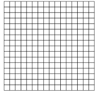
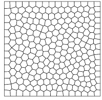
Figure 2: Examples of rectangular (left) and polygonal (Voronoi-like) (right) meshes composed of 256 cells.

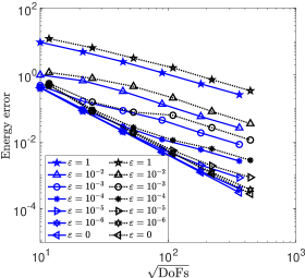
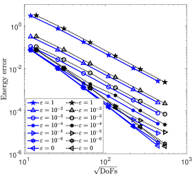
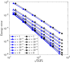
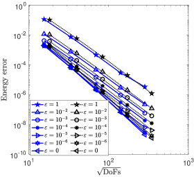
Figure 3: Polygonal domain and smooth solution. Convergence rates in the energy seminorm on rectangular (solid line) and polygonal (dotted line) meshes for different values of $\varepsilon$. The polynomial degree is $k=0$ (top left), $k=1$ (top right), $k=2$ (bottom left) and $k=3$ (bottom right).

We select $f$ and the boundary conditions on $\Omega:=(0,1)^{2}$ so that the exact solution to (1) is

$$u(x,y)=\sin(\pi x)^{2}\sin(\pi y)^{2}+e^{-(x-0.5)^{2}-(y-0.5)^{2}}.$$

We employ polynomial degrees $k\in\{0,\ldots,3\}$ and meshes consisting of $\{16,64,256,1024,4096,16384\}$ elements. The meshes can be either composed of rectangular cells or of polygonal (Voronoi-like) cells (generated through the PolyMesher Matlab library [22]). Two examples of rectangular and polygonal meshes, both composed of 256 cells, are shown in Figure 2. Despite an $hp$-error analysis falls beyond the present scope, we implement the stabilization terms in (20) and (21) with $h_{K}^{-1}$ replaced by $(k+1)^{2}h_{K}^{-1}$ for all $K\in\mathcal{T}_{h}$.

$\#$ Cells	$\varepsilon=1$	$\varepsilon=10^{-2}$	$\varepsilon=10^{-3}$	$\varepsilon=10^{-4}$	$\varepsilon=10^{-5}$	$\varepsilon=10^{-6}$	$\varepsilon=0$
		Rectangular meshes with $k=0$
64	0.85	0.52	1.41	1.93	2.03	2.04	2.04
256	0.94	1.01	0.89	1.62	1.92	1.97	1.97
1024	1.06	1.24	0.93	1.30	1.82	1.98	2.00
4096	1.10	1.22	1.25	1.00	1.55	1.92	2.00
16384	1.06	1.12	1.14	1.13	1.23	1.75	2.00
		Rectangular meshes with $k=1$
64	1.81	1.84	1.85	2.49	2.59	2.60	2.60
256	1.98	1.99	2.03	2.37	2.81	2.86	2.86
1024	2.01	2.01	2.08	1.99	2.71	2.93	2.96
4096	2.01	2.01	2.02	2.17	2.26	2.88	2.99
16384	2.01	2.01	2.01	2.06	2.08	2.61	2.99
		Rectangular meshes with $k=2$
64	2.65	2.68	2.84	3.26	3.49	3.52	3.53
256	2.85	2.85	2.92	3.19	3.68	3.80	3.82
1024	2.93	2.93	2.95	3.09	3.50	3.86	3.93
4096	2.97	2.97	2.97	3.02	3.24	3.74	3.97
16384	2.98	2.98	2.98	3.00	3.10	3.42	3.98
		Rectangular meshes with $k=3$
64	3.55	3.56	3.68	4.04	4.35	4.40	4.40
256	3.80	3.81	3.85	4.08	4.54	4.72	4.74
1024	3.91	3.91	3.92	4.02	4.37	4.79	4.88
4096	3.97	3.95	3.94	3.99	4.18	4.63	4.94

Table 1: Polygonal domain and smooth solution. Convergence rates in the energy seminorm on rectangular meshes for different values of $k$ and $\varepsilon$.

$\#$ Cells	$\varepsilon=1$	$\varepsilon=10^{-2}$	$\varepsilon=10^{-3}$	$\varepsilon=10^{-4}$	$\varepsilon=10^{-5}$	$\varepsilon=10^{-6}$	$\varepsilon=0$
		Rectangular meshes with $k=0$
64	1.40	0.17	2.36	2.92	2.94	2.94	2.94
256	1.76	1.36	0.52	2.81	2.95	2.96	2.96
1024	1.83	1.66	0.81	2.36	3.01	3.03	3.03
4096	1.90	1.84	1.75	0.74	2.97	3.02	3.03
16384	1.98	1.97	1.94	1.52	2.57	3.01	3.01
		Rectangular meshes with $k=1$
64	3.35	3.24	1.71	3.49	3.46	3.45	3.45
256	3.68	3.80	2.96	3.10	3.77	3.75	3.74
1024	3.84	3.94	3.78	1.98	3.90	3.89	3.87
4096	3.92	3.97	3.96	3.42	2.54	3.98	3.94
16384	4.05	4.02	4.01	3.93	2.69	3.92	3.97
		Rectangular meshes with $k=2$
64	4.51	4.60	4.32	4.42	4.37	4.36	4.36
256	4.77	4.81	4.72	4.57	4.74	4.70	4.69
1024	4.98	4.93	4.82	4.57	4.99	4.88	4.85
4096	2.49	4.17	4.92	4.83	4.69	5.02	4.97
		Rectangular meshes with $k=3$
64	5.29	5.26	5.05	5.12	5.21	5.20	5.19
256	5.87	5.87	5.59	5.37	5.66	5.62	5.61
1024	5.06	5.28	5.89	5.87	5.86	5.85	5.88

Table 2: Polygonal domain and smooth solution. Convergence rates in the $L^{2}$-norm on rectangular meshes for different values of $k$ and $\varepsilon$.

$\#$ Cells	$\varepsilon=1$	$\varepsilon=10^{-4}$	$\varepsilon=10^{-5}$	$\varepsilon=10^{-6}$	$\varepsilon=0$	2nd-order
		Rectangular meshes with $k=0$
1024	2.10e+06	8.44e+04	2.49e+05	3.13e+05	3.18e+05	2.47e+03
4096	3.38e+07	5.99e+05	6.15e+05	1.20e+06	1.33e+06	9.72e+03
16384	5.42e+08	6.84e+06	1.64e+06	3.84e+06	4.91e+06	3.85e+04
		Rectangular meshes with $k=1$
1024	2.52e+07	3.72e+05	4.34e+05	7.98e+05	8.82e+05	4.89e+03
4096	3.97e+08	4.86e+06	1.20e+06	2.44e+06	3.63e+06	1.92e+04
16384	6.29e+09	7.76e+07	9.84e+06	6.25e+06	1.49e+07	7.60e+04
		Rectangular meshes with $k=2$
1024	1.45e+08	2.04e+06	6.45e+05	1.75e+06	2.27e+06	9.29e+03
4096	2.28e+09	2.86e+07	1.20e+06	2.44e+06	9.30e+06	3.64e+04
16384	3.62e+10	4.52e+08	5.96e+07	1.02e+07	3.77e+07	1.44e+05
		Rectangular meshes with $k=3$
1024	4.77e+08	7.37e+06	1.40e+06	2.81e+06	4.88e+06	1.28e+04
4096	7.51e+09	9.59e+07	1.61e+07	5.77e+06	1.98e+07	5.04e+04
16384	1.19e+11	1.49e+09	2.02e+08	3.17e+07	8.01e+07	1.99e+05

Table 3: The condition number of condensed linear system on rectangular meshes for different values of $k$ and $\varepsilon$ for the proposed HHO method and the mixed order HHO method.

Let us first verify the convergence rates. We measure relative errors in the (broken) energy seminorm used on the left-hand side of our main error estimate (39). The errors are reported as a function of $\sqrt{\mathrm{DoFs}}$, where $\mathrm{DoFs}$ denotes the total number of globally coupled discrete unknowns (that is, the face unknowns). The results are reported in Figure 3. The first observation is that there is almost no difference in the convergence rates obtained on rectangular and polygonal meshes, and that these rates match the prediction of Theorem 4.5 for all the polynomial degrees. Next, we observe that the errors obtained with $\varepsilon=1$ and $\varepsilon=0$ converge, respectively, at the optimal rates $O(h^{k+1})$ and $O(h^{k+2})$, in agreement with Remark 4.6. For values of $\varepsilon$ between these two extreme values, a transition between the above two regimes is observed for $\varepsilon\approx h^{2}$. Whenever $\varepsilon\geq h^{2}$, the convergence rate is $O(h^{k+1})$ as expected for a fourth-order differential operator. Instead, whenever $\varepsilon\leq h^{2}$, the convergence rate is closer to the value $O(h^{k+2})$ expected for a second-order differential operator. In Table 1, we list the convergence rates on rectangular meshes (those on polygonal meshes lead to the same conclusions). Reading the table horizontally, the transition between the two regimes is clearly visible. For completeness, we also report the relative errors in the $L^{2}$-norm in Table 2. As for the energy seminorm error, there is almost no difference in the convergence rates obtained on rectangular and polygonal meshes, so that we focus on rectangular meshes. For $\varepsilon=0$, the convergence rate is always $O(h^{k+3})$ which is optimal (recall that polynomials of order $(k+2)$ are employed to approximate the traces on the mesh faces). For $\varepsilon=1$, the convergence rate is suboptimal for $k=0$, i.e., only $O(h^{2})$, as also observed with other nonconforming finite element methods applied to fourth-order PDEs. Instead, the optimal rate $O(h^{k+3})$ is recovered for $k\geq 1$. For $k=0$, a transition between second- and third-order convergence is observed as $\varepsilon\to 0$.

Finally, we present in Table 3 the (Euclidean) condition number of the linear system after static condensation for all the considered values of $\varepsilon$. To compare the value obtained for $\varepsilon=0$, we also report the condition number for the linear system discretized by a genuine HHO method for the second-order PDE, employing polynomials of order $(k+2)$ for the cell unknowns and $(k+1)$ for the face unknowns. The first observation is that the condition number for $\varepsilon=1$ scales as $\mathcal{O}(h^{-4})$ (as expected) and is larger than the condition number for all the other values of $\varepsilon$ by two orders of magnitude for all $k\geq 0$. Instead, for $\varepsilon=0$, the condition number scales as $\mathcal{O}(h^{-2})$ (again, as expected). In addition, the condition number for the genuinely second-order HHO method has the same quadratic scaling for the condition number, with values that are two orders of magnitude smaller than those reported in the column $\varepsilon=0$. This is reasonable since the proposed HHO method is not designed for genuinely second-order operators, but it still gives the optimal quadratic scaling for the condition number in the limit case $\varepsilon=0$. This encouraging observation indicates that the linear systems obtained with the present HHO method remain relatively well-behaved as $\varepsilon\to 0$. Further studies are, however, needed, including, e.g., preconditioned iterative methods (as, for instance, the one conducted in [20]). Finally, for decreasing $\varepsilon$ between the two extreme values $1$ and $0$, the condition number for fixed $k$ and $h$ decreases first and then increases. This nonmonotone behavior is probably related to the two different asymptotic regimes associated with $\varepsilon=1$ and $\varepsilon=0$.

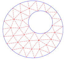
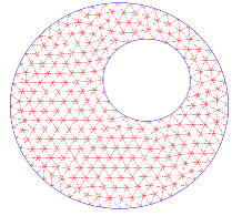
Figure 4: Two examples of curved triangular meshes with $65$ (left) and $527$ (right) cells fitting exactly the annular domain with a hole.

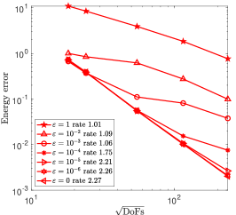
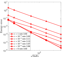
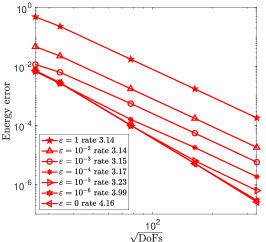
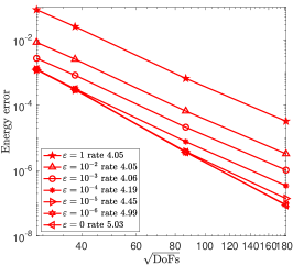
Figure 5: Annular domain and smooth solution. Convergence rates in the energy seminorm on curved triangular meshes for different values of $\varepsilon$. The polynomial degree $k=0$ (top left), $k=1$ (top right), $k=2$ (bottom left) and $k=3$ (bottom right).

5.2 Convergence rates and robustness in a domain with curved boundary

In this second example, we consider an annular domain constructed as the unit disc centered at the origin, with a circular hole centered at $(0.25,0.25)$ and with radius $0.4$; see Figure 4. We select $f$ and the boundary conditions so that the exact solution to (1) is

$$u(x,y)=(1+\sin(\pi(x^{2}+y^{2}-1)))e^{(-x^{2}-y^{2})}.$$

We consider a quasi-uniform sequence of triangular meshes composed of 65, 109, 527, 2266, and 9411 triangular elements. All the meshes fit the domain $\Omega$ exactly, and for every mesh in the sequence, each interior cell has only straight edges, whereas each boundary cell has one curved edge that exactly fits the boundary of $\Omega$.

We perform the same numerical experiment as in the previous section and report the results in Figure 5. The conclusions are the same as in the previous test case. The transition from the $O(h^{k+2})$ to the $O(h^{k+1})$ regimes is clearly visible in all cases.

5.3 Test case with boundary layer

Figure 6: Test case with boundary layer on the mesh composed of $9411$ cells, $\varepsilon=10^{-1}$ (top row) and $\varepsilon=10^{-3}$ (bottom row). Left column: reconstructed solution; middle column: piecewise gradient of reconstructed solution (Euclidean norm); right column: piecewise Hessian of reconstructed solution (Frobenius norm).

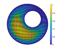
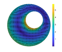
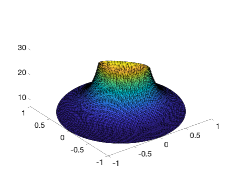
Figure 7: Test case with boundary layer on the mesh composed of $9411$ cells, $\varepsilon=10^{-6}$ (top row) and $\varepsilon=0$ (bottom row). Left column: reconstructed solution; middle column: piecewise gradient of reconstructed solution (Euclidean norm); right column: piecewise Hessian of reconstructed solution (Frobenius norm).

We conclude this series of numerical experiments with a somewhat more challenging test case featuring a boundary layer. We consider the same annular domain as in the previous section, we set the source term to $f:=10$ and we enforce homogeneous boundary conditions. The considered values for the singular perturbation parameter are $\varepsilon\in\{10^{-1},10^{-2},10^{-3},10^{-6},0\}$. In all cases, the analytical solution is unknown. Numerical solutions are obtained on the curved triangular meshes considered in the previous section using the polynomial degree $k=1$. We report in Figure 6 the reconstructed solution $R_{h}(\widehat{u}_{h})$ defined as $R_{h}(\widehat{u}_{h})|_{K}:=R_{K}(\widehat{u}_{K})$ for all $K\in\mathcal{T}_{h}$ (with $R_{K}(\widehat{u}_{K})$ defined just above Theorem 4.5), its piecewise gradient (Euclidean norm), and its piecewise Hessian (Frobenius norm) for $\varepsilon=10^{-1}$ and $\varepsilon=10^{-3}$ on the mesh composed of $9411$ curved triangular cells. Since $h=0.0344$ for this mesh, the boundary layer is well resolved for $\varepsilon=10^{-1}$ and barely resolved for $\varepsilon=10^{-3}$. Notice that $R_{h}(\widehat{u}_{h})$ is a piecewise cubic polynomial since we are using here $k=1$. We observe in Figure 6 that the presence of the boundary layer is reflected by larger values of the Hessian near the boundary, whereas the reconstructed solution and its piecewise gradient take moderate values. To illustrate that the HHO method remains stable even if the boundary layer is not resolved, we present in Figure 7 the same quantities as in Figure 6 obtained on the same mesh, but this time with $\varepsilon=10^{-6}$ and $\varepsilon=0$. We notice in particular that the larger values of the Hessian remain localized close to the boundary for $\varepsilon=10^{-6}$, whereas the solution to the second-order PDE is recovered for $\varepsilon=0$.

Finally, to give some insight on the resolution of the boundary layer for $\varepsilon\in\{10^{-1},10^{-2},10^{-3}\}$, we flag the mesh cells as belonging to the boundary layer by means of the following criterion:

$$\mathcal{T}_{h}^{*}:=\Big{\{}K\in\mathcal{T}_{h}\;\big{|}\;\|\nabla^{2}R_{K}(\widehat{u}_{K})\|_{L^{\infty}(K)}\geq\theta\max_{\widetilde{K}\in\mathcal{T}_{h}}\|\nabla^{2}R_{\widetilde{K}}(\widehat{u}_{\widetilde{K}})\|_{L^{\infty}(\widetilde{K})}\Big{\}},$$

with the threshold parameter set here to $\theta:=0.3$, and the $L^{\infty}$-norm estimated by computing the mean of the values taken by the Hessian norm at the three vertices of $K$. We report in Table 4 the two following quantities: (i) the maximal value of the Hessian, $\max_{\widetilde{K}\in\mathcal{T}_{h}}\|\nabla^{2}R_{\widetilde{K}}(\widehat{u}_{\widetilde{K}})\|_{L^{\infty}(\widetilde{K})}$; (ii) the area of the boundary layer, $\sum_{K\in\mathcal{T}_{h}^{*}}|K|$. First, we observe that the maximal value of the Hessian on the two finest meshes (which both resolve the boundary layer) are almost the same for all the values of $\varepsilon$. Moreover, the maximal value of the Hessian appears to scale as $\mathcal{O}(\varepsilon^{-\frac{3}{4}})$. This scaling is consistent with the expected scaling of the $H^{2}$-norm of the Hessian as $\mathcal{O}(\varepsilon^{-\frac{1}{2}})$ and a boundary layer with surface scaling as $\mathcal{O}(\varepsilon^{\frac{1}{2}})$. Furthermore, the set $\mathcal{T}_{h}^{*}$ covers a region whose area decays a bit slower than the expected rate $\mathcal{O}(\varepsilon^{\frac{1}{2}})$. This behavior indicates that somewhat finer meshes are still needed to fully resolve the geometric description of the boundary layer. This conclusion is corroborated in Figure 8, where we show the region covered by the cells in $\mathcal{T}_{h}^{*}$ for $\varepsilon\in\{10^{-1},10^{-2},10^{-3}\}$ and the curved triangular meshes composed of 2266, 9411, or 29496 cells. For $\varepsilon=0.1$, the set $\mathcal{T}_{h}^{*}$ contains not only cells close to the boundary but also cells in the interior. As $\varepsilon$ becomes smaller, the set $\mathcal{T}_{h}^{*}$ contains fewer and fewer cells in the interior of the domain, and for both $\varepsilon=10^{-2}$ and $10^{-3}$, the region covered by $\mathcal{T}_{h}^{*}$ is fully localized at the boundary. We notice, however, that even for $\varepsilon=10^{-3}$, there are boundary cells that are not flagged as members of $\mathcal{T}_{h}^{*}$; those cells are located in the part of the domain where the boundary of the inner disk is close to the boundary of the outer disk.

mesh	527 cells	2266 cells	9411 cells	29496 cells
$h$	0.1416	0.0704	0.0344	0.0205
	Max Hessian
$\varepsilon=10^{-1}$	6.94	7.09	7.11	7.11
$\varepsilon=10^{-2}$	38.13	40.48	40.88	41.22
$\varepsilon=10^{-3}$	88.63	128.33	147.96	151.32
	Area covered by $\mathcal{T}_{h}^{*}$
$\varepsilon=10^{-1}$	5.50e-01	4.51e-01	4.16e-01	3.86e-01
$\varepsilon=10^{-2}$	3.78e-01	2.47e-01	2.16e-01	2.13e-01
$\varepsilon=10^{-3}$	4.38e-01	1.65e-02	1.12e-01	1.22e-01

Table 4: Test case with boundary layer. Maximal Hessian value and area covered by $\mathcal{T}_{h}^{*}$ for $\varepsilon\in\{10^{-1},10^{-2},10^{-3}\}$ and the curved triangular meshes composed of 527, 2266, 9411, and 29496 cells.

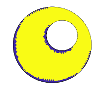
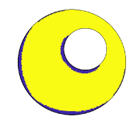
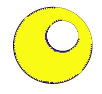
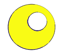
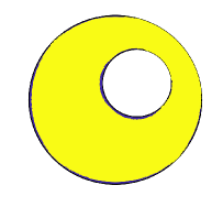
Figure 8: Region (blue color) covered by the cells in the set $\mathcal{T}_{h}^{*}$ for a mesh composed of $2266$ (left column), $9411$ (middle column), or 29496 cells, $\varepsilon=10^{-1}$ (top row), $\varepsilon=10^{-2}$ (middle row), or $\varepsilon=10^{-3}$ (bottom row).

6 Proof of main results

In this section, we present the proofs of Lemma 4.1, Lemma 4.3, Lemma 4.4, and Theorem 4.5.

6.1 Proof of Lemma 4.1

(1) We start with the lower bound in (28). Choosing the test function $w=v_{K}$ in (19) gives

$$\|\nabla{v}_{K}\|^{2}_{K,\varepsilon}={} (\nabla R_{K}^{\mathrm{i}}(v_{K}),\nabla v_{K})_{K,\varepsilon}+(v_{K}-v_{\partial K},\partial_{n}v_{K})_{\partial K^{\mathrm{i}}}+(v_{K},\partial_{n}v_{K})_{\partial K^{\mathrm{b}}}$$

$$-\varepsilon\Big{\{}(v_{K}-v_{\partial K},\partial_{n}\Delta v_{K})_{\partial K^{\mathrm{i}}}-(\partial_{n}v_{K}-\gamma_{\partial K},\partial_{nn}v_{K})_{\partial K^{\mathrm{i}}}-(\partial_{t}(v_{K}-v_{\partial K}),\partial_{nt}v_{K})_{\partial K^{\mathrm{i}}}$$

$$-(v_{K},\partial_{n}\Delta v_{K})_{\partial K^{\mathrm{b}}}+(\nabla v_{K},\nabla\partial_{n}v_{K})_{\partial K^{\mathrm{b}}}\Big{\}}.$$

Using the Cauchy–Schwarz inequality, the discrete inverse inequalities (8), (7), (9), and that $\partial_{nn}v_{K}\in\mathbb{P}^{k}(\partial K^{\mathrm{i}})$ to introduce the projection $\Pi_{\partial K^{\mathrm{i}}}^{k}$, we infer that

$$\|\nabla{v}_{K}\|_{K,\varepsilon}\leq\|\nabla R_{K}^{\mathrm{i}}(\widehat{v}_{K})\|_{K,\varepsilon}+C\Big{(}h_{K}^{-\frac{1}{2}}\|v_{K}-v_{\partial K}\|_{\partial K^{\mathrm{i}}}+h_{K}^{-\frac{1}{2}}\|v_{K}\|_{\partial K^{\mathrm{b}}}\\ +\varepsilon^{\frac{1}{2}}\Big{\{}h_{K}^{-\frac{3}{2}}\|v_{K}-v_{\partial K}\|_{\partial K^{\mathrm{i}}}+h_{K}^{-\frac{1}{2}}\|\Pi_{\partial K^{\mathrm{i}}}^{k}(\partial_{n}v_{K}-\gamma_{\partial K})\|_{\partial K^{\mathrm{i}}}+h_{K}^{-\frac{3}{2}}\|v_{K}\|_{\partial K^{\mathrm{b}}}+h_{K}^{-\frac{1}{2}}\|\nabla v_{K}\|_{\partial K^{\mathrm{b}}}\Big{\}}\Big{)}.$$

Since $\sigma_{K}=\max\{1,\varepsilon h^{-2}_{K}\}$, this implies that

$$\|\nabla{v}_{K}\|_{K,\varepsilon}\leq\|\nabla R_{K}^{\mathrm{i}}(\widehat{v}_{K})\|_{K,\varepsilon}+C\big{(}S^{\mathrm{i}}_{\partial K}(\widehat{v}_{K},\widehat{v}_{K})+S^{\mathrm{b}}_{\partial K}(v_{K},v_{K})\big{)}^{\frac{1}{2}}.$$

It remains to bound the four boundary terms on the right-hand side of (27). It is clear that

$$\sigma_{K}h_{K}^{-1}\|v_{\partial K}-v_{K}\|_{\partial K^{\mathrm{i}}}^{2}+\sigma_{K}h_{K}^{-1}\|v_{K}\|^{2}_{\partial K^{\mathrm{b}}}+\varepsilon h_{K}^{-1}\|\nabla v_{K}\|^{2}_{\partial K^{\mathrm{b}}}\leq S^{\mathrm{i}}_{\partial K}(\widehat{v}_{K},\widehat{v}_{K})+S^{\mathrm{b}}_{\partial K}(v_{K},v_{K}),$$

so that it only remains to bound ${\sigma_{K}}{h_{K}}\|\gamma_{\partial K}-\partial_{n}v_{K}\|_{\partial K^{\mathrm{i}}}^{2}$. To this purpose, using a Poincaré–Steklov inequality followed by a discrete trace inequality on $\partial K^{\mathrm{i}}$, we observe that

$$\sigma_{K}^{\frac{1}{2}}h_{K}^{\frac{1}{2}}\|\gamma_{\partial K}-\partial_{n}v_{K}\|_{\partial K^{\mathrm{i}}}\leq{} \sigma_{K}^{\frac{1}{2}}h_{K}^{\frac{1}{2}}\|\Pi_{\partial K^{\mathrm{i}}}^{k}(\gamma_{\partial K}-\partial_{n}v_{K})\|_{\partial K^{\mathrm{i}}}+\sigma_{K}^{\frac{1}{2}}h_{K}^{\frac{1}{2}}\|\partial_{n}v_{K}-\Pi_{\partial K^{\mathrm{i}}}^{k}(\partial_{n}v_{K})\|_{\partial K^{\mathrm{i}}}$$

$$\leq{} S^{\mathrm{i}}_{\partial K}(\widehat{v}_{K},\widehat{v}_{K})^{\frac{1}{2}}+C\sigma_{K}^{\frac{1}{2}}h_{K}^{\frac{3}{2}}\|\partial_{nt}v_{K}\|_{\partial K}$$

$$\leq{} S^{\mathrm{i}}_{\partial K}(\widehat{v}_{K},\widehat{v}_{K})^{\frac{1}{2}}+C\sigma_{K}^{\frac{1}{2}}h_{K}\|\nabla^{2}v_{K}\|_{K}.$$

The definition of $\sigma_{K}$ implies that $\sigma_{K}^{\frac{1}{2}}\leq 1+\varepsilon^{\frac{1}{2}}h_{K}^{-1}$, so that

$$\sigma_{K}^{\frac{1}{2}}h_{K}\|\nabla^{2}v_{K}\|_{K}\leq h_{K}\|\nabla^{2}v_{K}\|_{K}+\varepsilon^{\frac{1}{2}}\|\nabla^{2}v_{K}\|_{K}\leq C\|\nabla v_{K}\|_{K}+\varepsilon^{\frac{1}{2}}\|\nabla^{2}v_{K}\|_{K}\leq C\|\nabla v_{K}\|_{K,\varepsilon},$$

where we used the discrete inverse inequality (8). Owing to the above bound on $\|\nabla v_{K}\|_{K,\varepsilon}$, we infer that

$$\sigma_{K}^{\frac{1}{2}}h_{K}^{\frac{1}{2}}\|\gamma_{\partial K}-\partial_{n}v_{K}\|_{\partial K^{\mathrm{i}}}\leq C\Big{(}\|\nabla R_{K}^{\mathrm{i}}(\widehat{v}_{K})\|_{K,\varepsilon}+\big{(}S^{\mathrm{i}}_{\partial K}(\widehat{v}_{K},\widehat{v}_{K})+S^{\mathrm{b}}_{\partial K}(v_{K},v_{K})\big{)}^{\frac{1}{2}}\Big{)}.$$

Combining the above bounds, we conclude that the lower bound in (28) holds true.

(2) Let us now establish the upper bound in (28). This time we choose $w=R_{K}^{\mathrm{i}}(\widehat{v}_{K})$ in (19) and proceeding as above yields

$$\|\nabla R_{K}^{\mathrm{i}}(\widehat{v}_{K})\|_{K,\varepsilon}\leq\|\nabla{v}_{K}\|_{K,\varepsilon}+C\big{(}S^{\mathrm{i}}_{\partial K}(\widehat{v}_{K},\widehat{v}_{K})+S^{\mathrm{b}}_{\partial K}(v_{K},v_{K})\big{)}^{\frac{1}{2}}.$$

Moreover, it is clear that

$$S^{\mathrm{i}}_{\partial K}(\widehat{v}_{K},\widehat{v}_{K})+S^{\mathrm{b}}_{\partial K}(v_{K},v_{K})\leq\sigma_{K}h_{K}^{-1}\|v_{\partial K}-v_{K}\|_{\partial K^{\mathrm{i}}}^{2}+\sigma_{K}h_{K}\|\gamma_{\partial K}-\partial_{n}v_{K}\|_{\partial K^{\mathrm{i}}}^{2}\\ +\sigma_{K}h_{K}^{-1}\|v_{K}\|^{2}_{\partial K^{\mathrm{b}}}+\varepsilon h_{K}^{-1}\|\nabla v_{K}\|^{2}_{\partial K^{\mathrm{b}}},$$

since $\|\Pi^{k}_{\partial K^{\mathrm{i}}}(\partial_{n}v_{K}-\gamma_{\partial K})\|_{\partial K^{\mathrm{i}}}\leq\sigma_{K}h^{\frac{1}{2}}_{K}\|\partial_{n}v_{K}-\gamma_{\partial K}\|_{\partial K^{\mathrm{i}}}$. This completes the proof.

6.2 Proof of Lemma 4.3

(1) Let us first bound $\|v-\mathcal{E}_{K}(v)\|_{\sharp,K}$. The triangle inequality followed by the discrete inverse inequalities (7) and (8) implies that

$$\|v-\mathcal{E}_{K}(v)\|_{\sharp,K} \leq\|v-\Pi_{K}^{k+2}(v)\|_{\sharp,K}+\|\mathcal{E}_{K}(v)-\Pi_{K}^{k+2}(v)\|_{\sharp,K}$$

$$\leq\|v-\Pi_{K}^{k+2}(v)\|_{\sharp,K}+C\|\nabla(\mathcal{E}_{K}(v)-\Pi_{K}^{k+2}(v))\|_{K,\varepsilon},$$

so that we only need to bound the last term on the right-hand side. Straightforward algebra shows that, for all $\xi\in\mathbb{P}^{k+2}(K)$,

$$(\nabla\mathcal{E}_{K}(v)-\nabla\Pi_{K}^{k+2}(v),\nabla\xi)_{K,\varepsilon}={} -(\Pi_{K}^{k+2}(v)-v,\partial_{n}\xi)_{\partial K}$$

$$+\varepsilon\Big{\{}(\Pi_{K}^{k+2}(v)-v,\partial_{n}\Delta\xi)_{\partial K}-(\partial_{n}(\Pi_{K}^{k+2}(v)-v),\partial_{nn}\xi)_{\partial K}$$

$$-(\partial_{t}(\Pi_{K}^{k+2}(v)-\Pi^{k+2}_{\partial K^{\mathrm{i}}}(v)),\partial_{nt}\xi)_{\partial K^{\mathrm{i}}}-(\partial_{t}(\Pi_{K}^{k+2}(v)-v),\partial_{nt}\xi)_{\partial K^{\mathrm{b}}}\Big{\}}.$$

Choosing $\xi=\mathcal{E}_{K}(v)-\Pi_{K}^{k+2}(v)$ and using the discrete inverse inequalities (7), (8), (9) gives

$$\|\nabla(\mathcal{E}_{K}(v)-\Pi_{K}^{k+2}(v))\|_{K,\varepsilon}\leq{} C\Big{(}\sigma_{K}^{\frac{1}{2}}h_{K}^{-\frac{1}{2}}\|v-\Pi_{K}^{k+2}(v)\|_{\partial K}+\varepsilon^{\frac{1}{2}}h_{K}^{-\frac{1}{2}}\|\nabla(v-\Pi_{K}^{k+2}(v))\|_{\partial K}$$

$$+\varepsilon^{\frac{1}{2}}h_{K}^{-\frac{1}{2}}\|\partial_{t}(\Pi_{K}^{k+2}(v)-\Pi^{k+2}_{\partial K^{\mathrm{i}}}(v))\|_{\partial K^{\mathrm{i}}}\Big{)}.$$

The first two terms on the right-hand side are bounded using (15) and (16) leading to

$$\sigma_{K}^{\frac{1}{2}}h_{K}^{-\frac{1}{2}}\|v-\Pi_{K}^{k+2}(v)\|_{\partial K}+\varepsilon^{\frac{1}{2}}h_{K}^{-\frac{1}{2}}\|\nabla(v-\Pi_{K}^{k+2}(v))\|_{\partial K}\leq C\|\nabla(v-\Pi_{K}^{k+2}(v))\|_{K,\varepsilon}.$$

Moreover, for the last term on the right-hand side, proceeding as in [15], we invoke the discrete trace inequality (9) and observe that $\Pi_{K}^{k+2}(v)-\Pi^{k+2}_{\partial K^{\mathrm{i}}}(v)=\Pi^{k+2}_{\partial K^{\mathrm{i}}}(\Pi_{K}^{k+2}(v)-v)$. Since $\Pi^{k+2}_{\partial K^{\mathrm{i}}}$ is $L^{2}$-stable, we conclude that

$$\varepsilon^{\frac{1}{2}}h_{K}^{-\frac{1}{2}}\|\partial_{t}(\Pi_{K}^{k+2}(v)-\Pi^{k+2}_{\partial K^{\mathrm{i}}}(v))\|_{\partial K^{\mathrm{i}}}\leq C\varepsilon^{\frac{1}{2}}h_{K}^{-\frac{3}{2}}\|v-\Pi_{K}^{k+2}(v)\|_{\partial K^{\mathrm{i}}}.$$

Invoking (15), this yields

$$\varepsilon^{\frac{1}{2}}h_{K}^{-\frac{1}{2}}\|\partial_{t}(\Pi_{K}^{k+2}(v)-\Pi^{k+2}_{\partial K^{\mathrm{i}}}(v))\|_{\partial K^{\mathrm{i}}}\leq C\|\nabla(v-\Pi_{K}^{k+2}(v))\|_{K,\varepsilon}.$$

We have thus shown that

$$\|\nabla(\mathcal{E}_{K}(v)-\Pi_{K}^{k+2}(v))\|_{K,\varepsilon}\leq C\|\nabla(v-\Pi_{K}^{k+2}(v))\|_{K,\varepsilon}.$$

Putting the above bounds together shows that $\|v-\mathcal{E}_{K}(v)\|_{\sharp,K}\leq C\|v-\Pi_{K}^{k+2}(v)\|_{\sharp,K}$.

(2) Let us now bound $S^{\mathrm{i}}_{\partial K}(\mathcal{\widehat{I}}^{k}_{K}(v),\mathcal{\widehat{I}}^{k}_{K}(v))$. We have

$$S^{\mathrm{i}}_{\partial K}(\mathcal{\widehat{I}}^{k}_{K}(v),\mathcal{\widehat{I}}^{k}_{K}(v))={} \sigma_{K}h_{K}^{-1}\|\Pi^{k+2}_{\partial K}(v)-\Pi^{k+2}_{K}(v)\|^{2}_{\partial K^{\mathrm{i}}}+\sigma_{K}h_{K}\|\Pi^{k}_{\partial K^{\mathrm{i}}}(\Pi^{k}_{\partial K^{\mathrm{i}}}(\partial_{n}v)-\partial_{n}(\Pi^{k+2}_{K}(v)))\|^{2}_{\partial K^{\mathrm{i}}}$$

$$\leq{} \sigma_{K}h_{K}^{-1}\|v-\Pi^{k+2}_{K}(v)\|^{2}_{\partial K^{\mathrm{i}}}+\sigma_{K}h_{K}\|\partial_{n}(v-\Pi^{k+2}_{K}(v))\|^{2}_{\partial K^{\mathrm{i}}},$$

since $\Pi^{k+2}_{\partial K^{\mathrm{i}}}(\Pi^{k+2}_{K}(v))=\Pi^{k+2}_{K}(v)_{|\partial K^{\mathrm{i}}}$, $\Pi^{k+2}_{\partial K}$ is $L^{2}$-stable, and $\Pi^{k}_{\partial K^{\mathrm{i}}}\circ\Pi^{k}_{\partial K^{\mathrm{i}}}=\Pi^{k}_{\partial K^{\mathrm{i}}}$. The first term on the right-hand side is bounded by means of (16), yielding

$$\sigma_{K}h_{K}^{-1}\|v-\Pi^{k+2}_{K}(v)\|^{2}_{\partial K^{\mathrm{i}}} \leq C\|\nabla(v-\Pi_{K}^{k+2}(v))\|_{K,\varepsilon}^{2}.$$

Moreover, we have

$$\sigma_{K}h_{K}\|\partial_{n}(v-\Pi^{k+2}_{K}(v))\|^{2}_{\partial K^{\mathrm{i}}} \leq\varepsilon h_{K}^{-1}\|\partial_{n}(v-\Pi_{K}^{k+2}(v))\|^{2}_{\partial K^{\mathrm{i}}}+h_{K}\|\partial_{n}(v-\Pi_{K}^{k+2}(v))\|^{2}_{\partial K^{\mathrm{i}}}$$

$$\leq C\|\nabla(v-\Pi_{K}^{k+2}(v))\|_{K,\varepsilon}^{2}+h_{K}\|\partial_{n}(v-\Pi_{K}^{k+2}(v))\|^{2}_{\partial K^{\mathrm{i}}}$$

$$\leq C\|v-\Pi^{k+2}_{K}(v)\|_{\sharp,K}^{2},$$

where we used (15) and the definition of the $\|{\cdot}\|_{\sharp,K}$-norm. Putting the above bounds together, we infer that $S^{\mathrm{i}}_{\partial K}(\mathcal{\widehat{I}}^{k}_{K}(v),\mathcal{\widehat{I}}^{k}_{K}(v))\leq C\|v-\Pi^{k+2}_{K}(v)\|_{\sharp,K}^{2}$.

(3) Finally, let us bound $S^{\mathrm{b}}_{\partial K}(v-\Pi_{K}^{k+2}(v),v-\Pi_{K}^{k+2}(v))$. We have

$$S^{\mathrm{b}}_{\partial K}(v-\Pi_{K}^{k+2}(v),v-\Pi_{K}^{k+2}(v)) =\sigma_{K}h_{K}^{-1}\|v-\Pi_{K}^{k+2}(v)\|_{\partial K^{\mathrm{b}}}^{2}+\varepsilon h_{K}^{-1}\|\nabla(v-\Pi_{K}^{k+2}(v))\|_{\partial K^{\mathrm{b}}}^{2},$$

and the two terms on the right-hand side can be bounded by invoking the same arguments as in Step (2). This concludes the proof.

6.3 Proof of Lemma 4.4

Recalling the definition (31) of the lifting operator and the definition (21) of the boundary stabilization operator, we observe that

$$\ell_{h}(\widehat{w}_{h})=\sum_{K\in\mathcal{T}_{h}}\Big{\{}(f,w_{K})_{K}-(\nabla\mathcal{L}_{K}(u),\nabla R_{K}^{\mathrm{i}}(\widehat{w}_{K}))_{K,\varepsilon}+S_{\partial K}^{\mathrm{b}}(u,w_{K})\Big{\}}.$$

This implies that

$$\langle\delta_{h},\widehat{w}_{h}\rangle=\sum_{K\in\mathcal{T}_{h}}\Big{\{}(f,w_{K})_{K}-(\nabla\mathcal{E}_{K}(u),\nabla R_{K}^{\mathrm{i}}(\widehat{w}_{K}))_{K,\varepsilon}-S_{\partial K}^{\mathrm{i}}(\mathcal{\widehat{I}}^{k}_{K}(u),w_{K})-S_{\partial K}^{\mathrm{b}}(\Pi_{K}^{k+2}(u)-u,w_{K})\Big{\}}.$$ (42)

We bound the four terms on the right-hand side of (42). The first two terms are combined together by using that $f=\varepsilon\Delta^{2}u-\Delta u$, integration by parts, the regularity of the exact solution, and the definition of $R_{K}^{\mathrm{i}}(\widehat{w}_{K})$. Let us set $\eta|_{K}:=u|_{K}-\mathcal{E}_{K}(u|_{K})$ for all $K\in\mathcal{T}_{h}$. Proceeding as in [15] for the fourth-order operator and as in [14, 3] for the second-order operator, we obtain

$$\sum_{K\in\mathcal{T}_{h}}\Big{\{}(f,w_{K})_{K}-(\nabla\mathcal{E}_{K}(u|_{K}),\nabla R_{K}^{\mathrm{i}}(\widehat{w}_{K}))_{K,\varepsilon}\Big{\}}$$

$$=\sum_{K\in\mathcal{T}_{h}}\bigg{\{}(\nabla\eta,\nabla{w}_{K})_{K,\varepsilon}-\big{(}\partial_{n}\eta,w_{K}-w_{\partial K}\big{)}_{\partial K^{\mathrm{i}}}-\big{(}\partial_{n}\eta,w_{K}\big{)}_{\partial K^{\mathrm{b}}}$$

$$\quad+\varepsilon\Big{(}\big{(}\partial_{n}\Delta\eta,w_{K}-w_{\partial K}\big{)}_{\partial K^{\mathrm{i}}}-\big{(}\partial_{nn}\eta,\partial_{n}w_{K}-\chi_{\partial K}\big{)}_{\partial K^{\mathrm{i}}}-\big{(}\partial_{nt}\eta,\partial_{t}(w_{K}-w_{\partial K})\big{)}_{\partial K^{\mathrm{i}}}$$

$$\quad+\big{(}\partial_{n}\Delta\eta,w_{K}\big{)}_{\partial K^{\mathrm{b}}}-\big{(}\nabla\partial_{n}\eta,\nabla w_{K}\big{)}_{\partial K^{\mathrm{b}}}\Big{)}\bigg{\}}.$$

Invoking the Cauchy–Schwarz inequality and the discrete inverse inequalities from Lemma 2.3, we infer that

$$\sum_{K\in\mathcal{T}_{h}}\Big{\{}(f,w_{K})_{K}-(\nabla\mathcal{E}_{K}(u|_{K}),\nabla R_{K}^{\mathrm{i}}(\widehat{w}_{K}))_{K,\varepsilon}\Big{\}}\leq C\left(\sum_{K\in\mathcal{T}_{h}}\|\eta\|^{2}_{\sharp,K}\right)^{\frac{1}{2}}\|\widehat{w}_{h}\|_{\widehat{V}_{h}^{k}}.$$

Moreover, the third and fourth terms on the right-hand side of (42) are estimated by means of Lemma 4.3. Putting everything together concludes the proof.

6.4 Proof of Theorem 4.5

(1) Let us set $\widehat{e}_{h}^{k}:=\mathcal{\widehat{I}}_{h}^{k}(u)-\widehat{u}_{h}\in\widehat{V}_{h}^{k}$, so that $\widehat{e}_{K}^{k}:=\mathcal{\widehat{I}}_{K}^{k}(u|_{K})-\widehat{u}_{K}\in\widehat{V}_{K}^{k}$ for all $K\in\mathcal{T}_{h}$. The property (29) and the identity $a_{h}(\widehat{e}_{h}^{k},\widehat{e}_{h}^{k})=-\langle\delta_{h},\widehat{e}_{h}^{k}\rangle$ imply that

$$\alpha\sum_{K\in\mathcal{T}_{h}}\|\nabla(R_{K}^{\mathrm{i}}(\widehat{e}_{K}^{k}))\|_{K,\varepsilon}^{2}\leq\alpha\|\widehat{e}^{k}_{h}\|_{\widehat{V}_{h}^{k}}^{2}\leq a_{h}(\widehat{e}_{h}^{k},\widehat{e}_{h}^{k})=\langle\delta_{h},\widehat{e}_{h}^{k}\rangle.$$

Owing to the Lemma 4.4, we infer that

$$\sum_{K\in\mathcal{T}_{h}}\|\nabla(R_{K}^{\mathrm{i}}(\widehat{e}_{K}^{k}))\|_{K,\varepsilon}^{2}\leq C\sum_{K\in\mathcal{T}_{h}}\|u-\Pi_{K}^{k+2}(u)\|^{2}_{\sharp,K}.$$

By adding and subtracting $R_{K}^{\mathrm{i}}({\mathcal{\widehat{I}}_{K}^{k}(u|_{K})})$, we have

$$u_{|K}-R_{K}^{\mathrm{i}}(\widehat{u}_{K})-\mathcal{L}_{K}(u|_{K})=(u_{|K}-\mathcal{E}_{K}(u|_{K}))+R_{K}^{\mathrm{i}}(\widehat{e}_{K}^{k}).$$

Using the triangle inequality and Lemma 4.3, the error estimate (39) is derived.

(2) Let us assume that $u|_{K}\in H^{k+3}(K)$ for all $K\in\mathcal{T}_{h}$ if $k\geq 1$ and that $u|_{K}\in H^{4}(K)$ for all $K\in\mathcal{T}_{h}$ if $k=0$. Combining the multiplicative trace inequality (10) with the polynomial approximation result (11) shows that $\|u-\Pi_{K}^{k+2}(u)\|_{\sharp,K}\leq C\sigma_{K}^{\frac{1}{2}}h_{K}^{k+2}|u|_{H^{k+3}(K)}$ if $k\geq 1$ and $\|u-\Pi_{K}^{k+2}(u)\|_{\sharp,K}\leq C\sigma_{K}^{\frac{1}{2}}h_{K}^{k+2}(|u|_{H^{k+3}(K)}+h_{K}|u|_{H^{4}(K)})$ if $k=0$. Summing these estimates over the mesh cells and using the error estimate derived in Step (1) proves (40).

References

- [1] F. Bonaldi, D. A. Di Pietro, G. Geymonat, and F. Krasucki, A hybrid high-order method for Kirchhoff-Love plate bending problems, ESAIM Math. Model. Numer. Anal., 52 (2018), pp. 393–421.
- [2] S. C. Brenner and M. Neilan, A interior penalty method for a fourth order elliptic singular perturbation problem, SIAM J. Numer. Anal., 49 (2011), pp. 869–892.
- [3] E. Burman, M. Cicuttin, G. Delay, and A. Ern, An unfitted hybrid high-order method with cell agglomeration for elliptic interface problems, SIAM J. Sci. Comput., 43 (2021), pp. A859–A882.
- [4] E. Burman and A. Ern, An unfitted hybrid high-order method for elliptic interface problems, SIAM J. Numer. Anal., 56 (2018), pp. 1525–1546.
- [5] A. Cangiani, Z. Dong, and E. H. Georgoulis, -version discontinuous Galerkin methods on essentially arbitrarily-shaped elements, Math. Comp., (2021). Published online.
- [6] A. Cangiani, Z. Dong, E. H. Georgoulis, and P. Houston, hp-Version Discontinuous Galerkin Methods on Polygonal and Polyhedral Meshes, Springer, 2017.
- [7] K. L. Cascavita, F. Chouly, and A. Ern, Hybrid high-order discretizations combined with Nitsche’s method for Dirichlet and Signorini boundary conditions, IMA J. Numer. Anal., 40 (2020), pp. 2189–2226.
- [8] M. Cicuttin, A. Ern, and N. Pignet, Hybrid high-order methods. A primer with application to solid mechanics, SpringerBriefs in Mathematics, 2021.
- [9] B. Cockburn, D. A. Di Pietro, and A. Ern, Bridging the Hybrid High-Order and hybridizable discontinuous Galerkin methods, ESAIM Math. Model. Numer. Anal., 50 (2016), pp. 635–650.
- [10] M. Cui and S. Zhang, On the uniform convergence of the weak Galerkin finite element method for a singularly-perturbed biharmonic equation, J. Sci. Comput., 82 (2020), pp. 1–15.
- [11] D. Di Pietro and A. Ern, Mathematical aspects of discontinuous Galerkin methods, vol. 69 of Mathématiques & Applications (Berlin) [Mathematics & Applications], Springer, Heidelberg, 2012.
- [12] D. A. Di Pietro and J. Droniou, The hybrid high-order method for polytopal meshes: design, analysis, and applications, vol. 19, Springer Nature, 2020.
- [13] D. A. Di Pietro and A. Ern, A Hybrid High-Order locking-free method for linear elasticity on general meshes, Comput. Meth. Appl. Mech. Engrg., 283 (2015), pp. 1–21.
- [14] D. A. Di Pietro, A. Ern, and S. Lemaire, An arbitrary-order and compact-stencil discretization of diffusion on general meshes based on local reconstruction operators, Comput. Meth. Appl. Math., 14 (2014), pp. 461–472.
- [15] Z. Dong and A. Ern, Hybrid high-order and weak Galerkin methods for the biharmonic problem, arXiv preprint arXiv:2103.16404 (submitted), (2021).
- [16] A. Ern and J.-L. Guermond, Finite element quasi-interpolation and best approximation, ESAIM Math. Model. Numer. Anal. (M2AN), 51 (2017), pp. 1367–1385.
- [17] , Finite Elements II: Galerkin Approximation, Elliptic and Mixed PDEs, vol. 73 of Texts in Applied Mathematics, Springer Nature, Cham, Switzerland, 2021.
- [18] , Quasi-optimal nonconforming approximation of elliptic PDEs with contrasted coefficients and , , regularity, Found. Comput. Math. (Published online), (2021).
- [19] J. Guzmán, D. Leykekhman, and M. Neilan, A family of non-conforming elements and the analysis of Nitsche’s method for a singularly perturbed fourth order problem, Calcolo, 49 (2012), pp. 95–125.
- [20] X. Huang, Y. Shi, and W. Wang, A Morley–Wang–Xu element method for a fourth order elliptic singular perturbation problem, J. Sci. Comput., 87 (2021), pp. 1–24.
- [21] T. Nilssen and R. Tai, X.and Winther, A robust nonconforming -element, Math. Comp., 70 (2001), pp. 489–505.
- [22] C. Talischi, G. H. Paulino, A. Pereira, and I. F. M. Menezes, Polymesher: A general-purpose mesh generator for polygonal elements written in Matlab, Struct. Multidisc. Optim., 45 (2012), pp. 309–328.
- [23] A. Veeser and R. Verfürth, Poincaré constants for finite element stars, IMA J. Numer. Anal., 32 (2012), pp. 30–47.
- [24] L. Wang, Y. Wu, and X. Xie, Uniformly stable rectangular elements for fourth order elliptic singular perturbation problems, Num. Meth. Part. Diff. Eqs., 29 (2013), pp. 721–737.
- [25] M. Wang and X. Meng, A robust finite element method for a 3-D elliptic singular perturbation problem, J. Comput. Math., (2007), pp. 631–644.
- [26] M. Wang, J. Xu, and Y. Hu, Modified Morley element method for a fourth order elliptic singular perturbation problem, J. Comput. Math., (2006), pp. 113–120.
- [27] W. Wang, X. Huang, K. Tang, and R. Zhou, Morley-Wang-Xu element methods with penalty for a fourth order elliptic singular perturbation problem, Adv. Comp. Math., 44 (2018), pp. 1041–1061.
- [28] H. Wu and Y. Xiao, An unfitted -interface penalty finite element method for elliptic interface problems, J. Comput. Math., 37 (2019), pp. 316–339.
- [29] B. Zhang, J. Zhao, and S. Chen, The nonconforming virtual element method for fourth-order singular perturbation problem, Adv. Comp. Math., 46 (2020), pp. 1–23.
- [30] W. Zheng and H. Qi, On Friedrichs-Poincaré-type inequalities, J. Math. Anal. Appl., 304 (2005), pp. 542–551.