Resolving the fastest ejecta from binary Neutron Star mergers: implications for electromagnetic counterparts

Abstract

We examine the effect of spatial resolution on initial mass ejection in grid-based hydrodynamic simulations of binary neutron star mergers. The subset of the dynamical ejecta with velocities greater than $\sim 0.6$ c can generate an ultraviolet precursor to the kilonova on $\sim$ hr timescales and contribute to a years-long non-thermal afterglow. Previous work has found differing amounts of this fast ejecta, by one- to two orders of magnitude, when using particle-based or grid-based hydrodynamic methods. Here we carry out a numerical experiment that models the merger as an axisymmetric collision in a co-rotating frame, accounting for Newtonian self-gravity, inertial forces, and gravitational wave losses. The lower computational cost allows us to reach spatial resolutions as high as $4$ m, or $\sim 3\times 10^{-4}$ of the stellar radius. We find that fast ejecta production converges to within $10\%$ for a cell size of $20$ m. This suggests that fast ejecta quantities found in existing grid-based merger simulations are unlikely to increase to the level needed to match particle-based results upon further resolution increases. The resulting neutron-powered precursors are in principle detectable out to distances $\lesssim 200$ Mpc with upcoming facilities. We also find that head-on collisions at the free-fall speed, relevant for eccentric mergers, yield fast and slow ejecta quantities of order $10^{-2}M_{\odot}$, with a kilonova signature distinct from that of quasi-circular mergers.

1 Introduction

Detection of electromagnetic (EM) emission from neutron star (NS) mergers provides additional information beyond that contained in the gravitational wave (GW) signal, as was demonstrated for GW170817 (Abbott et al. 2017a). This information allows probing the merger environment (e.g., Levan et al. 2017; Blanchard et al. 2017), their use as standard sirens for cosmology (e.g., Abbott et al. 2017b), constraining their status as progenitors of short gamma-ray bursts (e.g., Abbott et al. 2017c), or assessing their contribution to the cosmic production of $r$-process elements (e.g., Cowperthwaite et al. 2017; Drout et al. 2017; Tanaka et al. 2017; Tanvir et al. 2017). Nucleosynthesis information is encoded in the kilonova signal, which arises from material ejected at subrelativistic speeds that is radioactively heated by freshily formed elements (Li & Paczyński 1998; Metzger et al. 2010).

The bulk of mass ejection in binary NS (BNS) mergers occurs in two ways. First, material is ejected on the dynamical time from the collision interface between the two stars or by tidal processes as the stars merge (e.g., Hotokezaka et al. 2013). Second, the accretion disk that forms after the merger ejects mass over longer timescales (see, e.g., Fernández & Metzger 2016 for a review). In both cases, the majority of the material is initially neutron-rich and moves at speeds $\lesssim 0.3$ c, which allows the $r$-process to proceed to completion, with a composition pattern that depends on the level of reprocessing by neutrinos (e.g., Wanajo et al. 2014; Just et al. 2015; Martin et al. 2015; Wu et al. 2016; Roberts et al. 2017; Lippuner et al. 2017). This results in a kilonova signal that peaks in the optical or infrared band and which evolves on a day to week timescale (Kasen et al. 2013; Tanaka & Hotokezaka 2013; Barnes & Kasen 2013; Fontes et al. 2015).

If a fraction of the ejected material expands on sufficiently short timescales, a freezout of the $r$-process can occur, with the ejecta consisting primarily of free, unprocessed neutrons that eventually undergo beta decay (Goriely et al. 2014). Freezout of neutrons requires the density to drop to $\sim 4\times 10^{5}$ g cm^-3 on timescales shorter than $\sim 5$ ms, which maps well to ejecta with velocities $\gtrsim 0.6$ c (Metzger et al. 2015). Such ejecta can also generate EM emission (Kulkarni 2005), and if launched ahead of slower material, can provide an ultraviolet precursor to the kilonova that evolves on a timescale of hours after the merger (Metzger et al. 2015). Detection of EM emission on a timescale of hours could have differentiated among various models that account for the kilonova from GW170817, but which diverge before the earliest EM observation at $\sim 11$ hours post-merger (Arcavi 2018).

The existence of sufficient ejecta with the required speed to generate a detectable neutron-powered precursor is not clear, however. A fast component with mass $\sim 10^{-4}\,{M_{\odot}}$ was first obtained in smoothed particle hydrodynamic (SPH) simulations of BNS mergers (Bauswein et al. 2013), but grid-based hydrodynamic simulations have found much smaller quantities ($\sim 10^{-7}-10^{-5}{M_{\odot}}$, e.g., Ishii et al. 2018,Radice et al. 2018), making a potential kilonova precursor much harder to detect given the expected distance to most sources ($\gtrsim 100$ Mpc) and current EM sensitivity limits.

More broadly, fast ejecta contributes to the non-thermal afterglow generated by outgoing mass interacting with the interstellar medium (Nakar & Piran 2011). In particular, fast ejecta has been proposed as a possible origin for the X-ray excess detected from GW170817 3 years after the merger (Hajela et al. 2021; Nedora et al. 2021). Small quantities ($\sim 10^{-8}-10^{-7}M_{\odot}$) of fast ejecta have also been proposed to account for the overall properties of the prompt gamma-ray burst emission from GW170817 via breakout of a jet from a rapidly-expanding cloud (Beloborodov et al. 2020). Finally, fast ejecta can also be produced in eccentric mergers, which can produce nearly head-on collisions at much higher radial velocities than in quasi-circular mergers (e.g., Gold et al. 2012; Chaurasia et al. 2018; Papenfort et al. 2018).

The reliability of ejecta masses from grid-based simulations is tied to how well the collision is spatially resolved, however. The spatial resolution of these simulations is usually limited by computational resources, with the finest grid spacings used to date being $63-86\rm m$ (Kiuchi et al. 2017). Properly resolving the surface layers of the star requires grid sizes $<10$ m (Kyutoku et al. 2014).

Here we perform a numerical experiment to assess the spatial resolution dependence of fast ejecta from the collision interface of BNS mergers in grid-based hydrodynamic simulations. To decrease the computational cost, we solve the Newtonian hydrodynamics equations in two-dimensional (2D) cylindrical symmetry with self gravity in a co-rotating frame, to account for orbital motion, and with an approximate prescription for orbital decay due to gravitational waves. These approximations, while losing accuracy relative to a full three-dimensional (3D) setting, preserve the qualitative feature of two sharp stellar edges colliding under the relevant force environment, and allow us to reach grid sizes as low as $4$ m ($\sim 3\times 10^{-4}$ of the NS radius).

The structure of the paper is the following. Section 2 describes our physical assumptions, computational method, and choice of models. Our results are presented in Section 3, with a general overview of our baseline model, parameter dependencies, and comparison with previous work. The observational implications of our results are presented in Section 4, and a summary and discussion follows in Section 5.

2 Methods

2.1 Physical Model and Approximations

Our goal is to study the ejection of material during the initial collision between the merging NSs and its immediate aftermath, with a focus on the high-velocity tail of the ejecta velocity distribution. Our numerical experiment attempts to capture the key features of the stellar collision in 2D, which allows for a much higher spatial resolution than is achievable in a full 3D configuration.

The hydrodynamic interaction between the two stars is influenced primarily by three effects: gravity, orbital motion, and orbital decay due to gravitational wave emission. Correspondingly, we neglect neutrino processes, magnetic fields, and stellar rotation in our study. While these effects can certainly influence mass ejection, they either provide sub-dominant corrections to the main processes considered here or, in the case of magnetic fields, introduce complications for comparing with previous work. Additionally, we do not keep track of the ejecta composition, and assess the feasibility of $r$-process freezout based on ejecta velocity, which is a good proxy for expansion time (Metzger et al. 2015).

We model the NS binary geometry in 2D by adopting an axisymmetric cylindrical coordinate system, positioning the stars along the symmetry ($\hat{z}$) axis, thereby accounting for their spherical geometry along the azimuthal ($\hat{\varphi}$) direction. We then set the orbital angular momentum vector aligned with the cylindrical radial ($\hat{r}_{\rm cyl}$) axis, with orbital motion occurring along a pseudo-azimuthal vector $\hat{\xi}=-{\rm sgn}(z)\hat{\varphi}$ around this axis (Figure 1).

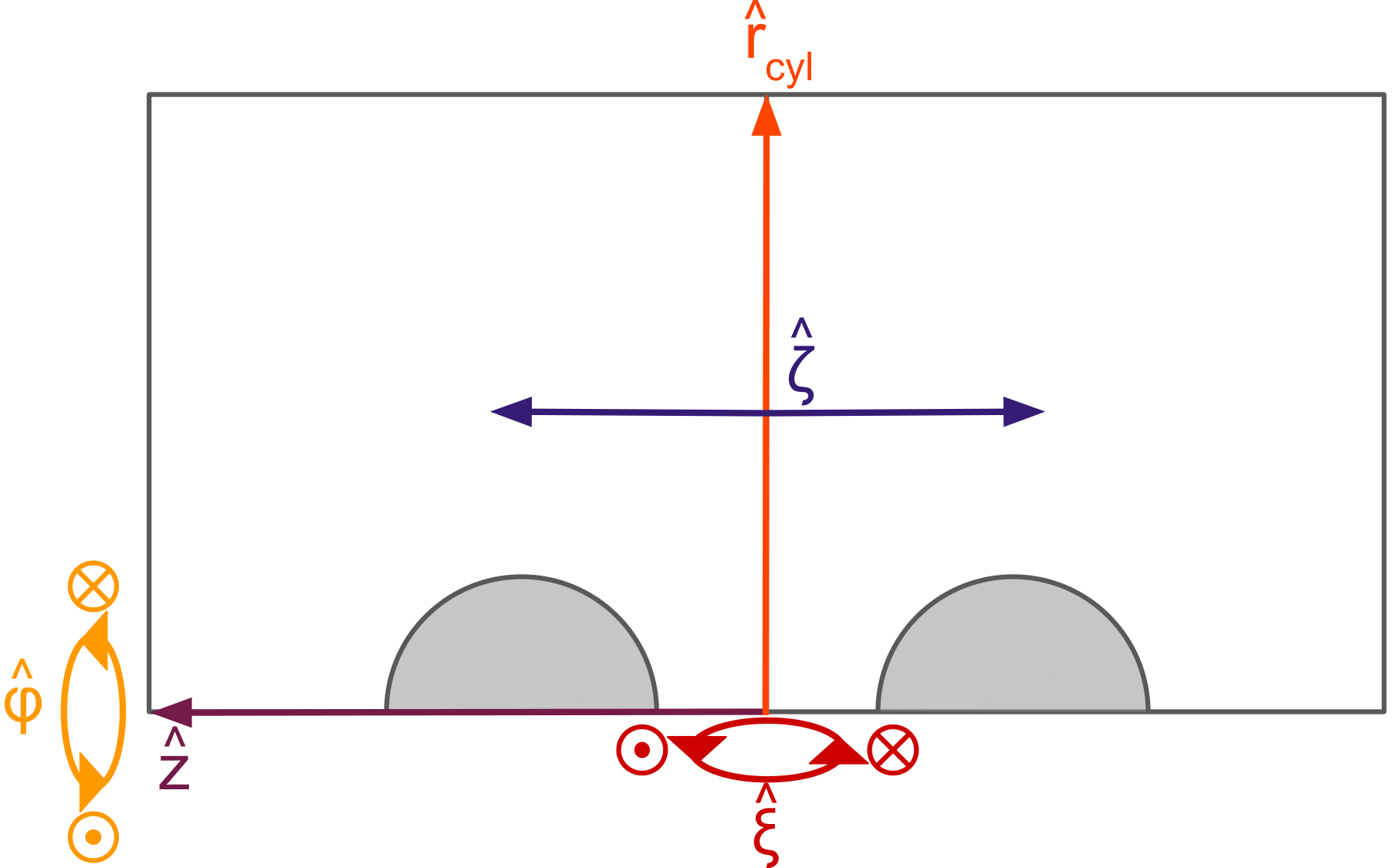
Figure 1: Schematic of the coordinate system used. An axisymmetric domain in cylindrical coordinates $(r_{\rm cyl},\varphi,z)$ is rotated $90^{\circ}$ counterclockwise and the stars are placed along the symmetry axis ($z$). The orbital angular momentum vector points in the cylindrical radial ($r_{\rm cyl}$) direction. Orbital motion occurs along the pseudo-azimuthal vector $\hat{\xi}=-{\rm sgn}(z)\hat{\varphi}$ and the distance from the rotation axis is described by the auxiliary vector $\hat{\zeta}={\rm sgn}(z)\hat{z}$.

Orbital motion is quantified with a specific angular momentum scalar $j=\omega z^{2}$, where $\omega(r_{\rm cyl},z,t)$ is the orbital angular velocity ($t$ is time). We work in a co-rotating coordinate system around $\hat{r}_{\rm cyl}$ with constant angular frequency $\omega_{0}=2\pi/t_{\rm dyn}$, where

$$t_{\rm dyn}=\left[\frac{4\pi^{2}}{G(M_{1}+M_{2})}d_{0}^{3}\right]^{1/2}$$ (1)

is the initial (Newtonian) orbital period of the system, with $d_{0}$ the initial separation between the stellar centers, and $M_{1,2}$ the stellar masses.

The centrifugal acceleration in this co-rotating frame is then

$$\mathbf{f}_{\rm cen}=\omega_{0}^{2}|z|\,\hat{\zeta}=\omega_{0}^{2}|z|{\rm sgn}(z)\,\hat{z}=z\omega_{0}^{2}\,\hat{z},$$ (2)

where $\hat{\zeta}={\rm sgn}(z)\,\hat{z}$ is a unit vector that points away from the orbital axis (Figure 1). The Coriolis acceleration is given by

$$\mathbf{f}_{\rm cor}=2\omega_{0}\left[v_{\xi}\hat{\zeta}-v_{\zeta}\hat{\xi}\right]=2\omega_{0}{\rm sgn}(z)\left[v_{\xi}\hat{z}-v_{z}\hat{\xi}\right],$$ (3)

where

$$v_{\xi}=\frac{j}{|z|}-|z|\omega_{0}$$ (4)

is the co-rotating frame velocity along $\hat{\xi}$, $v_{\zeta}={\rm sgn}(z)v_{z}$ is the speed away from the orbital angular momentum axis, and $v_{z}$ is the velocity along $\hat{z}$. With this formulation, matter moving toward the axis ($v_{\zeta}<0$) is accelerated in the $+\hat{\xi}$ direction, while matter rotating faster than the coordinate system ($v_{\xi}>0$) is pushed away from the rotation axis ($+\hat{\zeta}$), thus following the standard behavior of the Coriolis force. The azimuthal term in the Coriolis acceleration acts as a source term for the specific angular momentum

$$\left(\frac{\partial j}{\partial t}\right)_{\rm cor}=(\mathbf{r}\times\mathbf{f}_{\rm cor})_{r_{\rm cyl}}=-2\omega_{0}zv_{z}.$$ (5)

We neglect other components of the torque given the symmetry of our coordinate system (the $\zeta$ component of the Coriolis acceleration adds or subtracts from the centrifugal acceleration).

The correctness of this formulation is verified by the maintenance of a stable Keplerian orbit in the absence of gravitational wave losses (Section 2.2). A schematic of the relative direction of the inertial accelerations is shown in Figure 2.

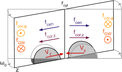
Figure 2: Schematic of the numerical experiment. A corotating frame is employed, with constant angular velocity $\omega_{0}$ set to the initial Keplerian value. Matter thus experiences centrifugal and Coriolis accelerations (equations 2-3). Orbital motion is quantified with a space- and time-dependent specific angular momentum scalar $j=\omega z^{2}$, which can be modified by the component of the Coriolis acceleration in the orbital direction (equation 5) and by gravitational wave emission (equation 16). The stars with masses $M_{1}$ and $M_{2}$ are initialized at an initial separation $d_{0}$ measured from their centers, with the center of mass at the origin, and with velocities in the $z$-direction toward the rotation axis, resulting in the acceleration directions shown. The intrinsic symmetry of the cylindrical coordinate system accounts for the sphericity of the stars.

2.2 Numerical Hydrodynamics

We use FLASH version 4.5 (Fryxell et al. 2000; Dubey et al. 2009) to solve the equations of Newtonian hydrodynamics in 2D cylindrical coordinates in a co-rotating frame, with source terms due to self-gravity and gravitational wave losses:

$$\frac{\partial\rho}{\partial t}+\nabla\cdot(\rho\mathbf{v}) = 0$$ (6)

$$\frac{D\mathbf{v}}{Dt} = -\frac{\nabla P}{\rho}-\nabla\Phi+\mathbf{f}_{\rm cen}+(\mathbf{f}_{\rm cor}\cdot\hat{\zeta})\hat{\zeta}$$ (7)

$$\frac{Dj}{Dt} = \left(\frac{\partial j}{\partial t}\right)_{\rm gw}+\left(\frac{\partial j}{\partial t}\right)_{\rm cor}$$ (8)

$$\frac{D\epsilon}{Dt}-\frac{P}{\rho^{2}}\frac{D\rho}{Dt} = 0$$ (9)

$$\nabla^{2}\Phi = 4\pi G\rho$$ (10)

where $D/Dt\equiv(\partial/\partial t+\mathbf{v}\cdot\nabla)$, $\mathbf{v}=v_{\rm rcyl}\hat{r}_{\rm cyl}+v_{z}\hat{z}$ is the poloidal velocity, $\rho$ is the density, $P$ is the total gas pressure, $\epsilon$ is the total specific internal energy, $\Phi$ is the gravitational potential, and $G$ is the gravitational constant. The system of equations is solved with the dimensionally-split Piecewise-Parabolic Method (PPM; Colella & Woodward 1984), the multipole self-gravity solver of Couch et al. (2013), and is closed with a piecewise polytropic equation of state (EOS).

The EOS contains a cold component with 4-segments

$$P_{{\rm c},i}=K_{i}\rho^{\Gamma_{i}}\qquad i=\{0,1,2,3\},$$ (12)

where the adiabatic indices $\Gamma_{i}$, transition densities $\rho_{i}$, and transition pressure $P_{\rm c,1}$ are taken from Read et al. (2009). This cold component connects continuously at low density to a SLy EOS for the crust (Douchin & Haensel 2001). The EOS also includes a thermal component (e.g., Bauswein et al. 2010), such that the total pressure satisfies

$$P = P_{\rm c}+P_{\rm th}$$ (13)

$$P_{\rm th} = (\Gamma_{\rm th}-1)\rho\epsilon_{\rm th}$$ (14)

$$\epsilon_{\rm th} = \epsilon-\epsilon_{\rm c}.$$ (15)

where the subscripts “c” and “th” denote the cold and thermal components, respectively. We adopt $\Gamma_{\rm th}=5/3\simeq 1.67$ as an intermediate value in the interval $[1.5,2]$, which was found by Bauswein et al. (2010) to bracket the behavior of micro-physical, finite-temperature EOS’s.

We include the effect of gravitational wave losses on the orbit through a source term that modifies the specific angular momentum

$$\left(\frac{\partial j}{\partial t}\right)_{\rm gw}=\frac{1}{2}\frac{j}{d}\left(\frac{\partial d}{\partial t}\right)_{\rm gw}$$ (16)

where we assume a Keplerian dependence on the instantaneous orbital separation $d$ between the centers of mass of each star (semimajor axis of the reduced mass), $j\propto d^{1/2}$. The rate of change of $d$ is taken to be the standard expression for two point masses with $e=0$ (Peters 1964),

$$\left(\frac{\partial d}{\partial t}\right)_{\rm gw}=-\frac{64}{5}\frac{G^{3}}{c^{5}}\frac{(M_{1}+M_{2})M_{1}M_{2}}{d^{3}}.$$ (17)

While these equations are strictly valid only for point masses, we apply this source term to all stellar material that has non-zero $j$ (i.e., material ejected after the collision). Once $j$ reaches zero, the source term is also set to zero. For equal-mass binaries, we set $d=2|z|$ in equations (16) and (17). For asymmetric binaries, we need to account for the mass ratio $q=M_{2}/M_{1}$, and hence set $d=(1+1/q)|z_{1}|$ or $d=(1+q)|z_{2}|$ for all matter on the side of star 1 or star 2 relative to $z=0$, respectively. Aside from this substitution, the mass ratio dependence scales out of equation (16).

The computational domain spans the range $[0,90]$ km in $r_{\rm cyl}$ and $[-90,90]$ km in $z$, and is discretized with a uniform grid with square cells $\Delta r_{\rm cyl}=\Delta z$. We choose our resolution in relation to the pressure scale height $H_{\rm p}=P/(\rho|\nabla\Phi|)$ near the stellar surface (Figure 3). Given the numerical dissipation properties of PPM (e.g., Porter & Woodward 1994), we consider a length scale as resolved if we can cover it with 10 computational cells. Our baseline grid spacing is $\Delta r_{\rm cyl}=\Delta z=32$ m in all models (Section 2.3), which resolves the pressure scale height out to $\sim 93\%$ of the stellar radius. Our finest resolution, $\Delta r_{\rm cyl}=\Delta z=4$ m, reaches beyond 99.9% of the stellar radius $R_{\rm ns}$, enclosing all but the outermost $\sim 9\times 10^{-4}M_{\odot}$ of the stellar mass.

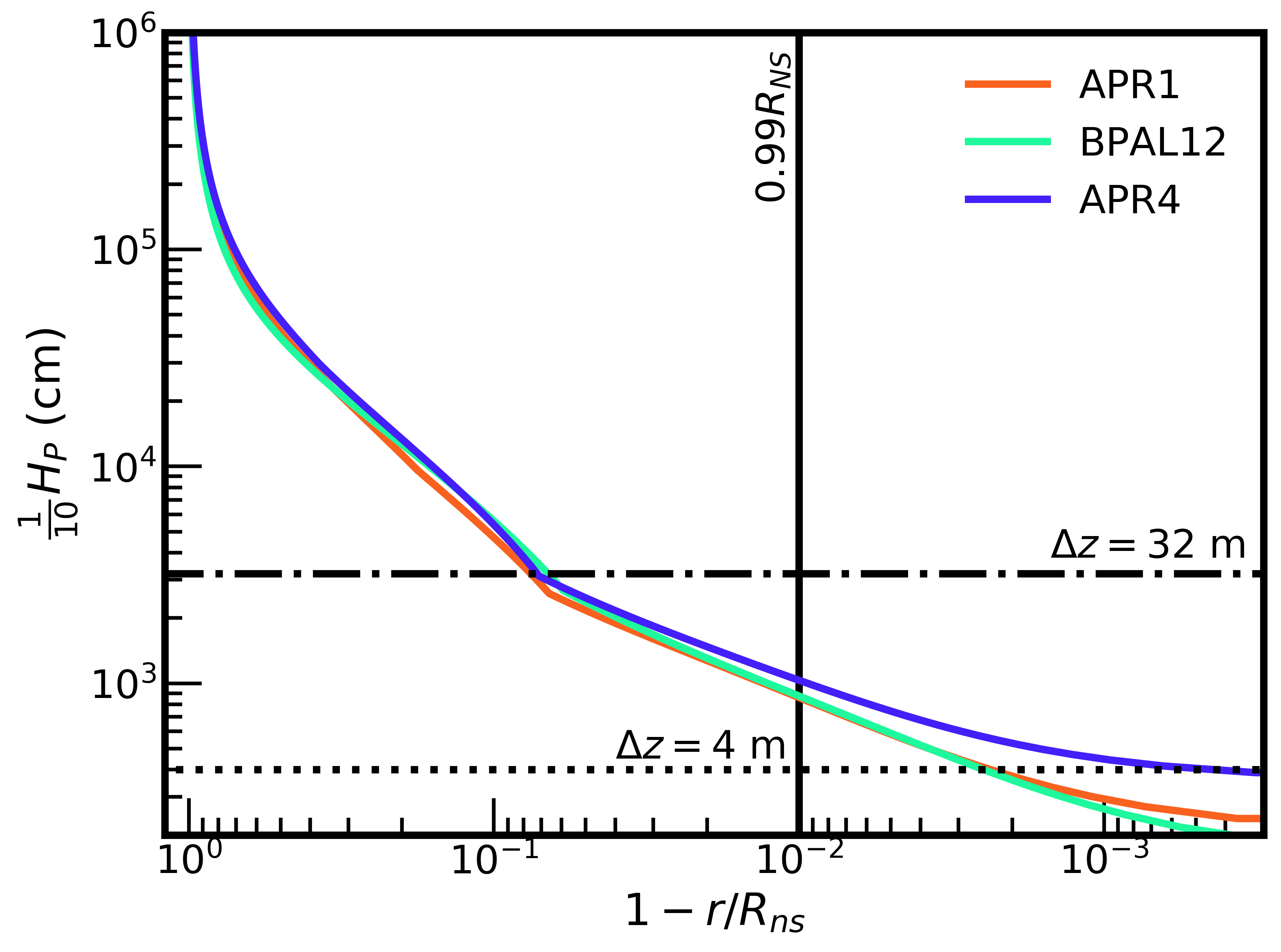
Figure 3: Spatial resolution in terms of relevant length scales in the problem. Solid curves show $1/10$th of the pressure scale height $H_{\rm p}$ as a function of exterior radius in a $1.4M_{\odot}$ NS constructed with the APR4 EOS (purple), BPAL12 EOS (teal), and APR1 EOS (orange). Also shown as horizontal lines are our baseline resolution $\Delta r_{\rm cyl}=\Delta z=32$ m (dot-dashed) and the finest resolution used, $\Delta r_{\rm cyl}=\Delta z=4$ m (dotted). The latter covers $H_{p}$ with $10$ cells out to $>99.9\%$ of the stellar radius, corresponding to an exterior mass of $<9\times 10^{-4}{M_{\odot}}$ for the APR4 EOS.

The boundary conditions are reflecting at $r_{\rm cyl}=0$, and outflow at all other domain limits. The orbital configuration is tested by initializing the stars in a Keplerian orbit, with an initial separation $d_{0}\simeq 8R_{\rm ns}$, and verifying that the stars maitain their initial positions in the absence of gravitational wave losses, with only minor in-place oscillations. Based on this stationarity test we employ $128$ multipoles for self-gravity in all of our runs.

2.3 Initial Conditions

Neutron stars are constructed by solving the Newtonian hydrostatic equilibrium equations using the EOSs described in Section 2.2. We test the solution by evolving an isolated star centered at the origin for $10$ stellar dynamical times $\tau^{\rm ns}_{\rm dyn}\simeq(2\pi)^{-1}(R_{\rm NS}/d_{0})^{3/2}\,t_{\rm dyn}$, and verifying that it remains close to a steady-state with low kinetic energy (Figure 4).

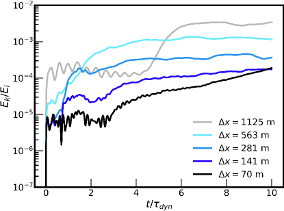
Figure 4: Hydrostatic equilibrium test of an isolated $1.4M_{\odot}$ NS constructed with the APR4 EOS at the center of the computational domain, showing the ratio of kinetic energy $E_{\rm k}$ to internal energy $E_{\rm i}$ in stellar material as a function of time, in units of the dynamical time of the star $\tau_{\rm dyn}\simeq 0.07$ ms. Curves correspond to different spatial resolutions, as labeled.

Simulations are initialized with the two stellar centers placed on the $z$-axis at a separation $d_{0}$ slightly larger than the sum of the stellar radii, and located such that the center of mass of the system is at the origin, $|z_{1}/z_{2}|=M_{2}/M_{1}=q$, with $|z_{1}|$ and $|z_{2}|$ the initial $z$ coordinates of the corresponding stellar centers

In our default configuration, the interior of each star is assigned the Keplerian velocity of the center of mass uniformly, with a correction for the inspiral of the orbit, thus initially $v_{\xi}\simeq 0$ at the center of mass of each star. The initial velocity along the $z$ axis is set to the value implied by the decay rate of the orbital separation due to gravitational wave emission (equation 17), with a characteristic magnitude $\sim 2\times 10^{9}$ cm s^-1. To probe the sensitivity of our results to the initial conditions, we also evolve a head-on collision model that removes rotation, intertial forces, and gravitational wave losses, as well as one that sets the velocity along the $z$ axis to the free-fall value.

The stars are initially embedded in an ambient medium of mass $\sim 2.3\times 10^{-8}{M_{\odot}}$, density $10^{4}~{}\rm{g}/\rm{cm}^{3}$, and constant pressure $10^{25}~{}\rm{dyn}/\rm{cm}^{2}$, with the remaining thermodynamic variables determined by the EOS. The ambient mass is negligible relative to characteristic ejecta masses of interest, and hence it should not significantly influence the velocity of this ejecta.

Table 1: Models evolved and results.

Model	EOS	Inertial Force	$M_{1}$	$M_{2}$	$R_{\rm 1.4}$	$\Delta x$	$M_{\rm ej}$	$M_{v\geq 0.6c}$			$E_{k}$
		Treatment						total	contact	orbital	$>0.3c$	$>0.6c$
			(${M_{\odot}}$)	(${M_{\odot}}$)	(km)	(m)	(${M_{\odot}}$)		(${M_{\odot}}$)		($10^{49}$ erg)
base	APR4	All forces	1.4	1.4	12.6	32	$2.5\times 10^{-5}$	$1.4\times 10^{-5}$	$1.3\times 10^{-5}$	$6.6\times 10^{-8}$	$1.0$	$0.83$
R281*						281.3	$1.9\times 10^{-5}$	$8.0\times 10^{-6}$	$8.0\times 10^{-6}$	$6.4\times 10^{-8}$	$0.57$	$0.35$
R141*						140.6	$2.7\times 10^{-5}$	$1.5\times 10^{-5}$	$1.5\times 10^{-5}$	$1.8\times 10^{-8}$	$1.0$	$0.79$
R70*						70.3	$2.8\times 10^{-5}$	$1.5\times 10^{-5}$	$1.5\times 10^{-5}$	$6.3\times 10^{-8}$	$1.2$	$0.98$
R16						16.0	$2.2\times 10^{-5}$	$1.1\times 10^{-5}$	$1.1\times 10^{-5}$	$1.0\times 10^{-7}$	$0.98$	$0.78$
R4						4.0	$2.6\times 10^{-5}$	$1.2\times 10^{-5}$	$1.2\times 10^{-5}$	$1.2\times 10^{-7}$	$1.0$	$0.77$
APR1	APR1				11.0	32	$5.4\times 10^{-5}$	$2.6\times 10^{-5}$	$2.6\times 10^{-5}$	$5.4\times 10^{-7}$	$2.6$	$2.1$
BPAL12	BPAL12				14.1		$1.4\times 10^{-6}$	$1.3\times 10^{-8}$	$1.3\times 10^{-8}$	$1.1\times 10^{-10}$	$0.02$	$0.0006$
OR	APR4	On rails			12.6		$1.3\times 10^{-2}$	$5.7\times 10^{-3}$	$2.2\times 10^{-3}$	$3.6\times 10^{-3}$	$430$	$300$
OR70						70.3	$1.6\times 10^{-2}$	$6.4\times 10^{-3}$	$1.9\times 10^{-3}$	$4.5\times 10^{-3}$	$520$	$360$
OR141						140.6	$1.3\times 10^{-2}$	$7.0\times 10^{-3}$	$1.7\times 10^{-3}$	$5.3\times 10^{-3}$	$460$	$360$
FF		Free-fall				32	$3.6\times 10^{-2}$	$1.2\times 10^{-2}$	$1.5\times 10^{-4}$	$1.2\times 10^{-2}$	$950$	$530$
FF70						70.3	$3.2\times 10^{-2}$	$9.1\times 10^{-3}$	$2.0\times 10^{-4}$	$8.9\times 10^{-3}$	$830$	$410$
FF141						140.6	$3.9\times 10^{-2}$	$1.1\times 10^{-2}$	$2.0\times 10^{-4}$	$1.1\times 10^{-2}$	$940$	$510$
M1.2_1.2		All forces	1.2	1.2		32.0	$1.9\times 10^{-5}$	$8.2\times 10^{-6}$	$8.2\times 10^{-6}$	$2.5\times 10^{-8}$	$0.74$	$0.53$
M1.7_1.7			1.7	1.7			$5.0\times 10^{-5}$	$2.5\times 10^{-5}$	$2.5\times 10^{-5}$	$8.0\times 10^{-7}$	$1.9$	$1.5$
M1.5_1.3			1.5	1.3			$2.7\times 10^{-4}$	$2.7\times 10^{-5}$	$2.7\times 10^{-5}$	$5.1\times 10^{-7}$	$5.1$	$1.2$
M1.6_1.2			1.6	1.2			$2.5\times 10^{-4}$	$1.4\times 10^{-5}$	$1.2\times 10^{-5}$	$1.6\times 10^{-6}$	$4.5$	$0.61$

Note: Columns from left to right show model name, EOS, inertial force setup as defined in Section 2.3, NS masses, radius of a $1.4{M_{\odot}}$ NS, cell size ($\Delta z=\Delta r_{\rm cyl}$), total unbound mass ejected, fast ($v_{r}\geq 0.6$ c) unbound ejecta, cumulative kinetic energy of matter travelling at $v_{r}>0.3$ c and similarily for $v>0.6$ c. The latter is shown in the last 3 columns as total amount, and broken up by angular direction. Ejecta masses represent cumulative amounts launched by the end of the default simulation time (1.6 ms). Models marked with a star (low-resolution) were evolved for 10 times longer than the rest of the set.

2.4 Models Evolved

Table LABEL:tab:models shows all of our models and their initial parameters. Our baseline case consists of two NSs with equal mass $M_{1}=M_{2}=1.4M_{\odot}$ built with the APR4 EOS (Akmal et al. 1998), yielding a radius $R_{\rm ns}=12.6$ km. This lies within the radius range allowed by GW170817 (Abbott et al. 2018), thus yielding a realistic compactness. The default spatial resolution is $\Delta r_{\rm cyl}=\Delta z=32$ m, and the default evolution time is $\simeq 1.2\,t_{\rm dyn}$ (equation 1), corresponding to $1.6$ ms. This time interval is sufficient to achieve complete ejection of fast material in our simulations.

To probe the effect of spatial resolution, the fiducial configuration is also evolved at grid spacings $\Delta z=\{281,141,70\}$ m, which overlap with values used in previous 3D numerical relativity simulations of BNS mergers. The lower computational cost of these models allow us to evolve them for $\simeq 12\,t_{\rm dyn}$, or $16$ ms. Two high-resolution models that employ $\Delta z=\{16,4\}$ m are evolved for $\simeq 1.2t_{\rm dyn}$ to test for convergence.

We probe the effect of varying the EOSs – and thus the compactness of the NSs – with two models that use APR1 (Akmal et al. 1998) and BPAL12 (Zuo et al. 1999), which yield neutron star radii $11$ km and $14.1$ km for a stellar mass $1.4M_{\odot}$, respectively. All other simulation parameters (aside from the initial separation, which depends on the stellar radius) are identical to those in the default configuration.

Likewise, we probe the effect of our force prescription by evolving two models that remove rotation, inertial forces, and gravitational wave losses from the baseline configuration. In one case (model OR, ‘on rails’), we leave the initial collision velocity along $z$ unchanged from the baseline configuration, corresponding to the rate of decay of the orbital separation by gravitational waves (§2.2). The other model (FF) sets the collision velocity to the free-fall speed. Both of these models are evolved at the default resolution as well as at coarser grid sizes $\Delta z={141,70}$ m, to probe the sensitivity to mass ejection to this parameter (models OR70, OR141, FF70, and FF141).

The effect of changing the total binary mass at constant mass ratio is studied with models M1.2_1.2 and M1.7_1.7, which set the total mass to $1.2+1.2\,M_{\odot}$ and $1.7+1.7M_{\odot}$, respectively. We ignore here the possibility of prompt collapse, which is possible for the model with the highest total mass. Models M1.5_1.3 and M1.6_1.2 keep the total mass constant at $2.8{M_{\odot}}$, but change the mass ratio to $q=0.87$ ($1.5{M_{\odot}}+1.3{M_{\odot}}$) and $q=0.75$ ($1.6{M_{\odot}}+1.2{M_{\odot}}$), respectively. The initial stellar positions and velocities of these asymmetric cases are consistent with the description in Section 2.3.

3 Results

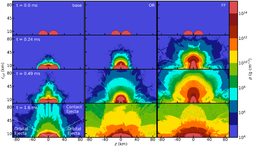
Figure 5: Left: Snapshots in the evolution of the base model (c.f. Table LABEL:tab:models), showing mass density at various times, as labeled. The white dotted line at $30^{\circ}$ from the $z$-axis shows the division between contact plane and orbital plane directions, as labeled. Middle: Same as in the left column but removing orbital motion, inertial forces, and gravitational wave losses (model OR). Right: A head-on collision at the free-fall speed (model FF), for comparison.

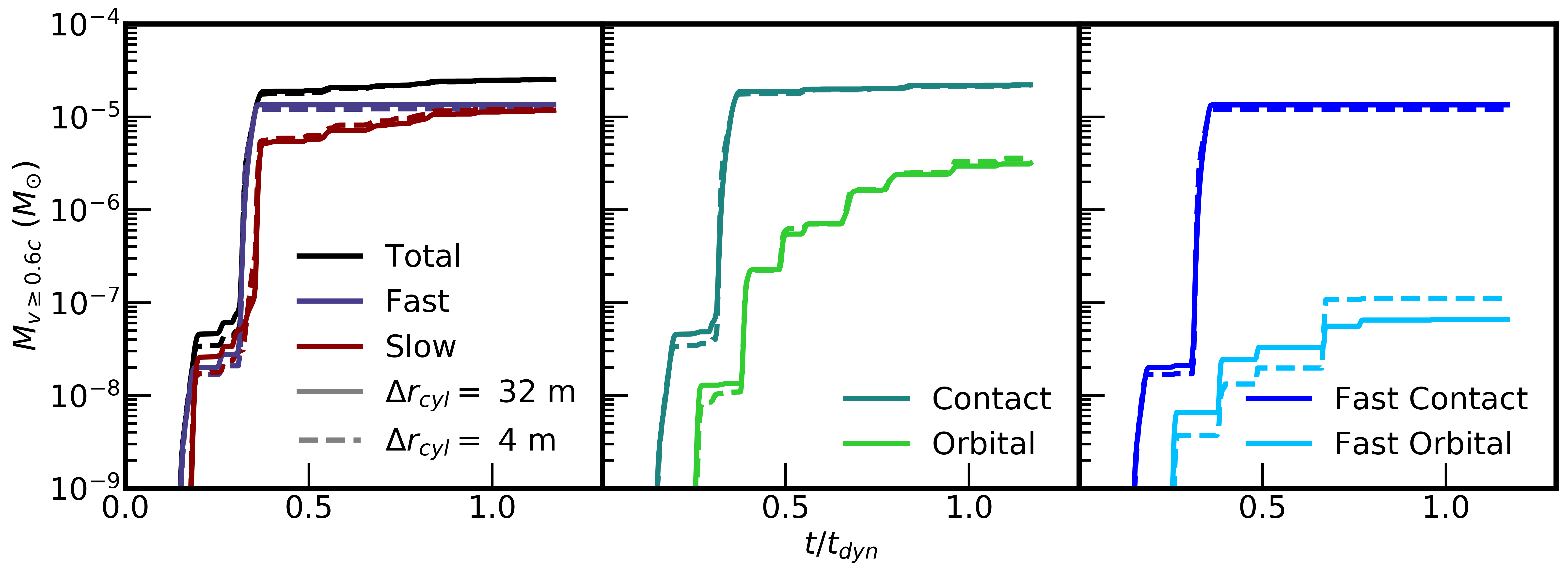
Figure 6: Time-dependence of mass ejection in model base (solid lines) and R4 (dashed lines, highest resolution), as measured from a spherical sampling surface with a radius $30$ km from the origin. Left: Unbound ejecta separated into fast ($v>0.6$ c) and slow ($v<0.6$ c). Middle: Total unbound ejecta separated into angular directions (c.f. Figure 5). Right: Fast ejecta separated into angular directions.

3.1 Overview of baseline model and resolution dependence

As the stars collide, mass is ejected on a timescale of $\sim 1$ ms, first in the general direction of the rotation axis, and then toward equatorial regions, as shown in the left row of Figure 5. For analysis, we divide the ejection directions into contact plane and equatorial plane by a surface $30^{\circ}$ from the $z$-axis (the contact plane being the region that includes the rotation axis). Ejected material is considered unbound from the system when it has positive Bernoulli parameter:

$${\rm Be}=\frac{1}{2}\mathbf{v}^{2}+\epsilon+\frac{P}{\rho}+\Phi>0.$$ (18)

We sample the unbound mass flux at a spherical extraction radius $r_{\rm out}=30$ km from the origin (the $z$-axis is the symmetry axis for the mass ejection measurement sphere). Fast ejecta is defined as that with radial velocity $v>0.6$ c at $r=r_{\rm out}$, while slow ejecta is that with $v<0.6$ c.

Mass ejection is episodic (Figure 6), with two initial bursts of mostly fast ejecta, up to a time of $\sim 0.4\,t_{\rm dyn}\simeq 0.5$ ms. Thereafter, slow ejecta continues to build up beyond $\sim 1\,t_{\rm dyn}\simeq 1.4$ ms. Each of these episodes is the result of oscillations in the collision remnant, as seen in global 3D merger simulations (e.g., Bauswein et al. 2013). These oscillations show as steps in the cumulative ejected mass as a function of time in Figure 6. While contact plane ejecta appears in only two bursts, with marginal increases thereafter, orbital plane ejecta gradually builds up through several oscillations, with the average velocity of the ejected material decreasing with time. The vast majority of the fast ejecta is launched toward the contact plane direction in this model.

Note that on the timescale of our simulation, production of fast ejecta is largely complete, while the slow ejecta is still increasing (Figure 6). We thus find total ejecta masses (fast and slow) that are significantly lower than those typically reported in global 3D merger simulations for this binary combination ($\gtrsim 10^{-3}M_{\odot}$; e.g., Hotokezaka et al. 2013, Rosswog 2013, Lehner et al. 2016, Sekiguchi et al. 2016, Bovard et al. 2017, Dietrich et al. 2017, Radice et al. 2018)

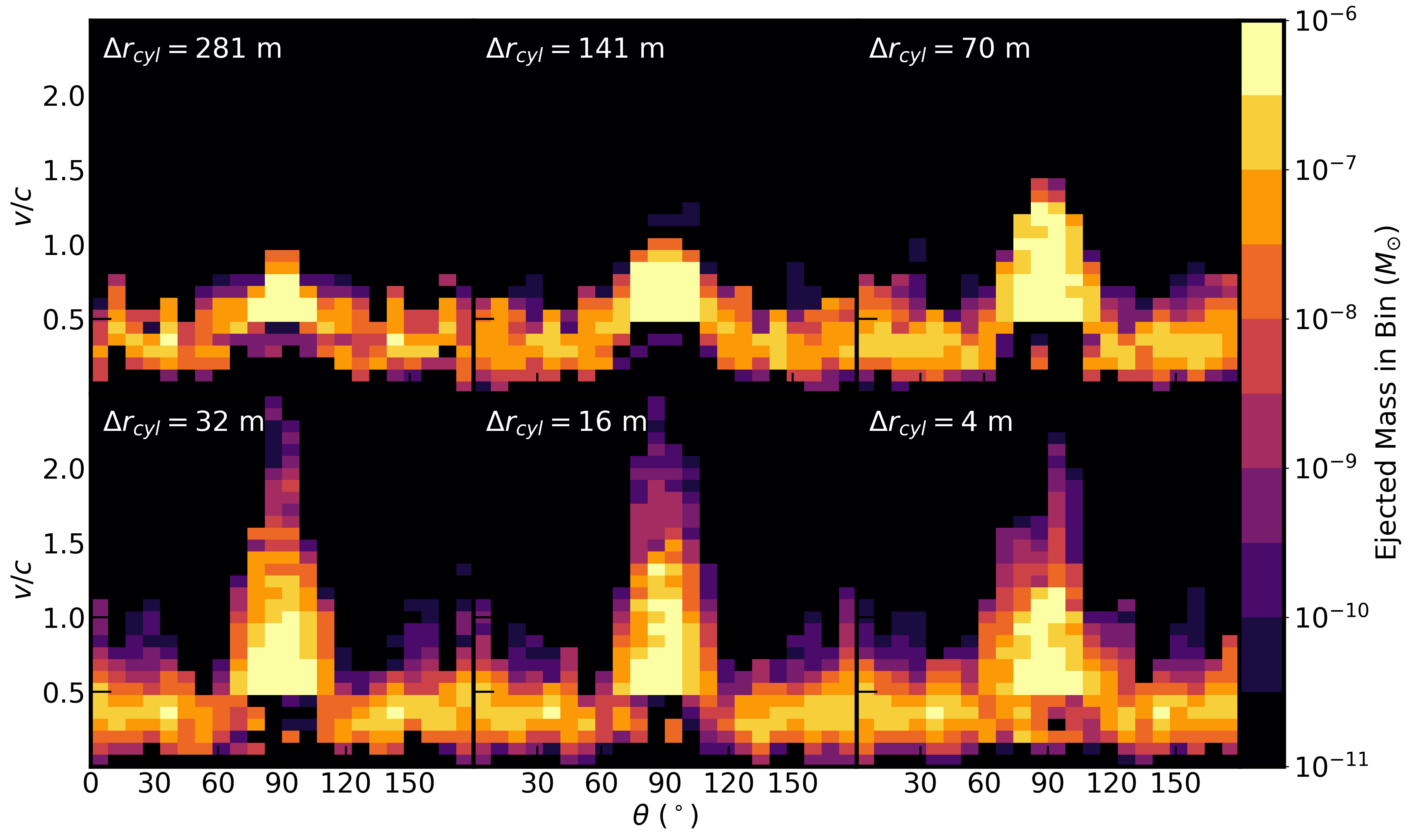
Figure 7: Mass histogram of unbound ejecta as a function of ejection polar angle (measured from the $z$-axis, c.f. Figure 5, $90^{\circ}$ corresponds to the rotation axis) and velocity, for our default binary configuration. Different panels correspond to different spatial resolutions, as labeled (c.f. Table LABEL:tab:models, the panel for $\Delta r_{\rm cyl}=32$ m corresponds to the base model). Since our simulations are Newtonian, a small amount of mass can achieve speeds larger than the speed of light.

Figure 6 also shows that the mass ejection history is qualitatively the same in the baseline model and in the highest resolution model (R4). In particular, the contact plane ejecta is the same within $10\%$. While larger changes with resolution up to a factor $\sim 2$ are seen in the fast material ejected toward equatorial latitudes, this contribution is subdominant compared to matter ejected toward the contact plane.

The effect of spatial resolution on the angle- and velocity distribution of cumulative unbound ejecta is shown in Figure 7. This sequence of models spans a factor of $\simeq 70$ in resolution, from the coarsest grid size $\Delta r_{\rm cyl}\simeq 280$ m to the finest value at $4$ m. While the overall shape of these two-dimensional histograms is the same in all cases, the most visible change occurs for matter within $\sim 30^{\circ}$ of the rotation axis, i.e. contact plane ejecta. As the resolution is increased, more mass is ejected around the rotation axis at the high- and low velocity ends. Note that since our simulations are Newtonian, a small amount of mass achieves $v>c$.

Taking the fast ejecta from model R4 as a baseline, we estimate the degree of convergence of mass ejection by computing differences relative to this ejecta value as a function of resolution. Figure 8 shows that the total fast ejecta mass converges as $\Delta r_{cyl}^{0.46}$ over the entire resolution range explored. Convergence to within $10\%$ is achieved for $\Delta r_{cyl}\approx 19.7$ m.

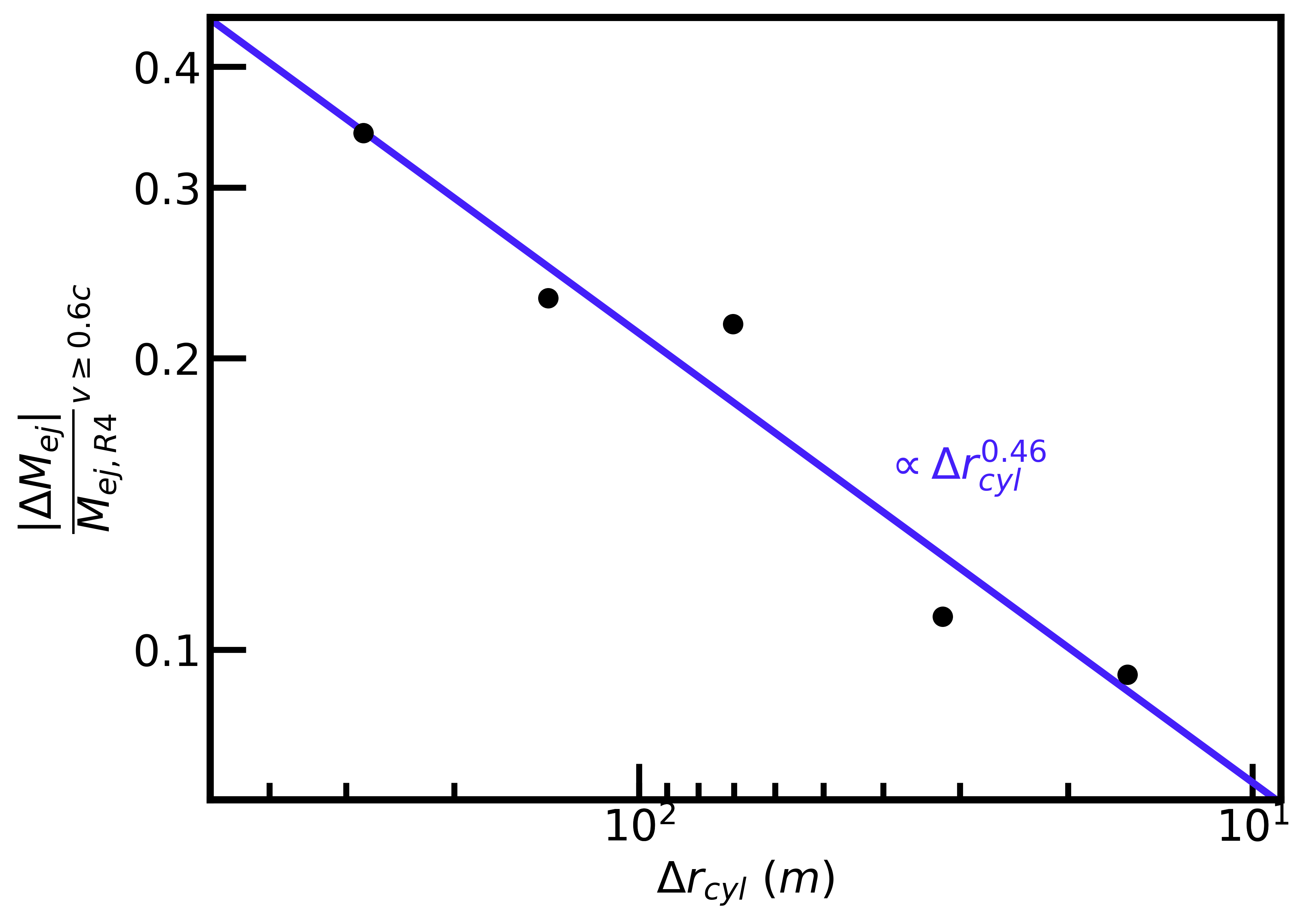
Figure 8: Convergence of fast ejecta mass with spatial resolution. Shown are relative differences in total fast ejecta mass relative to that from model R4. The purple line is a power-law fit.

A natural explanation of this trend with cell size is the increasing degree by which the stellar edges are resolved (Figure 3). Overall, fast ejecta on the contact plane can change by a factor of $\sim 2$ from the lowest to highest resolution (Table LABEL:tab:models). The equatorial ejecta also increases by a factor of $\sim 2$ over the entire resolution range. Spatial resolution therefore also has an effect on matter ejected during remnant oscillations (as inferred from Figure 6) even though the overall shape of the equatorial ejecta distribution remains largely the same in Figure 7. Again, equatorial ejecta contributes primarily with $v<0.6$ c in this model.

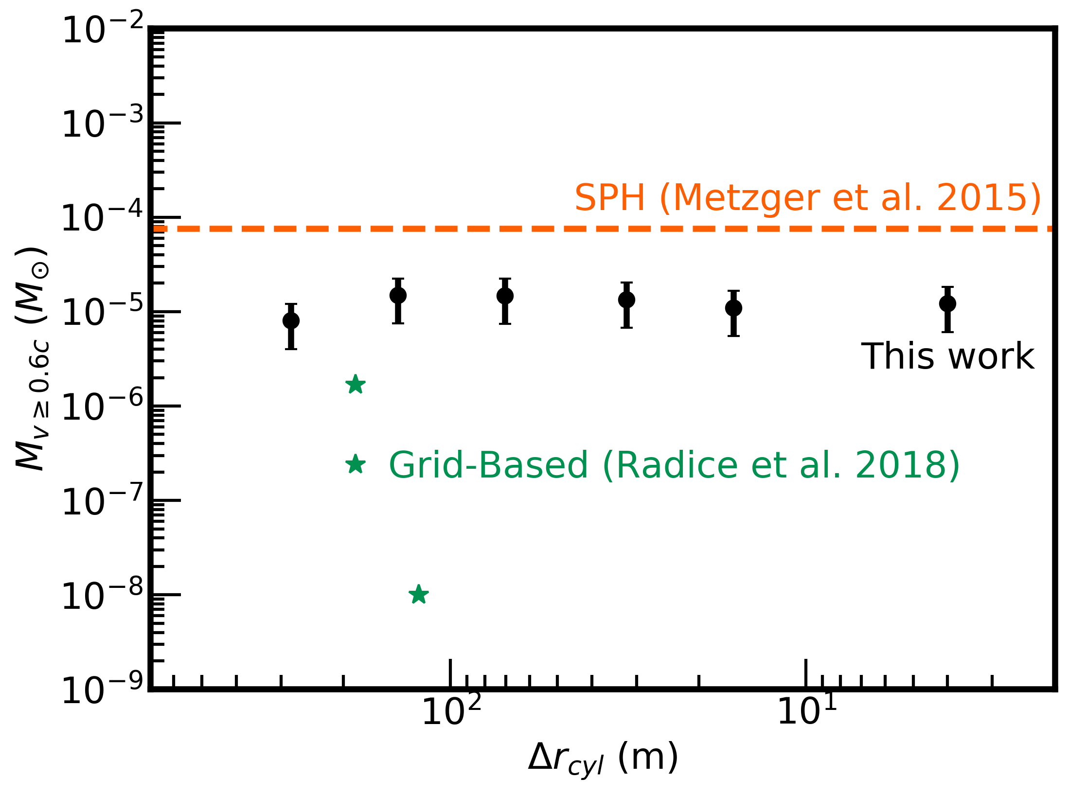
Figure 9: Total fast ejecta for our default configuration (black circles) as a function of cell size (c.f. Table LABEL:tab:models). The orange dashed line shows the $r$-process freezout ejecta reported in Metzger et al. (2015) out of the equal-mass $1.35{M_{\odot}}$ merger simulation from Bauswein et al. (2013), carried out with an SPH code without neutrinos and the DD2 EOS. Green stars show the fast ejecta reported in Radice et al. (2018) for a set of models with the closest parameters to our base case: an equal-mass $1.35{M_{\odot}}$ binary simulated with a grid code and the DD2 EOS. The resolutions and neutrino treatment are, from top to bottom, $185$ m with an M0 scheme, $185$ m with a leakage scheme, and $123$ m with a leakage scheme, respectively. We estimate that our values have a measurement uncertainty of a factor $\sim 2$ due to sensitivity to the extraction radius and the imposition of a velocity cut at $0.6$ c to estimate free neutron masses (§3.4).

The total fast ejecta from our default configuration across the resolution range we explore is shown in Figure 9, where the very mild dependence with resolution is apparent. For comparison, we also show fast ejecta results from the grid-based, global 3D merger simulations of Radice et al. (2018), corresponding to equal-mass $1.35M_{\odot}$ binaries evolved with different resolutions and neutrino prescriptions. Our results suggest that the fast ejecta values from Radice et al. (2018) are already close to convergence, and are unlikely to increase (for higher resolution) by the magnitude required to match the amount inferred by Metzger et al. (2015) from the SPH simulations of Bauswein et al. (2013).

We also note that the initial burst in the base model ejects $\sim 10^{-8}-10^{-7}M_{\odot}$ (Figure 6), which has similar magnitude to the ultrarelativistic envelope envisioned by Beloborodov et al. (2020) as a breakout medium for the jet in order to account for the features of the prompt emission in GRB170817A. We caution that for these small amounts of mass, other processes such as neutrino emission and absorption (as envisioned by Beloborodov et al. (2020) to power the expanding envelope) or magnetic fields can be dynamically important and are missing in our simulations. Also, the mass in ambient medium in our models is $\sim 10^{-8}M_{\odot}$ (Section 2.3), hence the first burst of ejecta is slowed down significantly and its final velocity in our simulations is not physical. Nevertheless, our results suggest the possibility that such a fast moving envelope of small mass could arise from the hydrodynamic interaction alone. Properly capturing this phenomenon will require highly-resolved global simulations with neutrino transport and magnetic fields.

3.2 Dependence on force prescription and collision velocity

As an attempt to quantify the uncertainty in the approximations used in our numerical experiment, we evolve a model (OR) in which we remove the corotation of the coordinate system: no orbital motion, and therefore no centrifugal and Coriolis forces (Section 2.1), as well as no gravitational wave losses (Section 2.2). The setting is thus a head-on collision at a speed set by the decay of the semimajor axis due to gravitational waves (equation 17).

Figure 5 compares the evolution of model OR with our base case. Mass ejection occurs at a faster pace, and spans a broader range of latitudes. Ejecta is produced in an episodic manner, with two main bursts occurring during the simulated time, like in model base. The second burst is more temporally spread than the first burst in the base case, however. Also, while in the latter model both bursts of fast ejecta are predominantly launched toward the contact plane, in model OR the first burst is launched toward the contact plane and the second toward the orbital plane. We also note that model OR produces more slow ejecta than fast ejecta.

Table LABEL:tab:models shows that the total fast ejecta is a factor $\sim 300$ larger in model OR than in the base case, with a comparable separation between contact and equatorial plane directions. While the total ejecta mass shows a non-monotonic dependence on spatial resolution, the fast component does vary monotonically, with contact plane ejecta increasing and orbital plane ejecta decreasing with finer grid spacing, and such that the total fast ejecta decreases by $\sim 20\%$ when going from $\Delta z=141$ m to $32$ m. Lacking the suppressing effect of centrifugal forces, we can take model OR as an absolute upper limit to the fast ejecta generated from a binary neutron star collision.

For reference, we also consider a head-on collision at the free-fall speed (model FF). Such a calculation has a long history, and the qualitative result is well-known (e.g., Shapiro 1980; Rasio & Shapiro 1992; Centrella & McMillan 1993; Ruffert & Janka 1998; Kellerman et al. 2010). This type of collision is astrophysically relevant in the context of eccentric mergers, in which head-on or off-center encounters are a common outcome (e.g., Gold et al. 2012; Chaurasia et al. 2018; Papenfort et al. 2018)

Figure 5 shows that model FF behaves in a qualitatively similar way to model OR, but due to the higher collision speed, mass ejection occurs at a faster rate. Material first decelerates in the collisional direction as the density gradients meet. The strong pressure gradients produced accelerate material in the contact plane, expanding in that direction before collapsing back and then expanding in the orbital plane direction (e.g, Centrella & McMillan 1993). Over longer time periods, the remnant oscillates in a pattern that alternates between the contact and orbital planes, before settling into a spherical remnant. Model FF exhibits two such oscillations of the collision remnant during the $1.6$ ms evolution time, resulting in a series of periodic fast ejecta bursts first toward the contact plane, then toward the orbital plane, with the production of fast ejecta saturating before the end of the simulation. We do not follow the oscillation of the remnant for long enough to fully capture all slow ejecta produced, however, which is typically launched by 4-6 violent oscillations of the remnant, before settling into a spherical shape over a period of $\sim 3$ ms (Ruffert & Janka 1998).

Table LABEL:tab:models shows that mass ejection from model FF is significant, with a total fast ejecta reaching $0.01M_{\odot}$. Like in model OR, the total unbound ejecta shows a non-monotonic dependence on resolution. While the fast ejecta produced toward the contact plane decreases by $\sim 25\%$ for increasing resolution, fast ejecta launched toward the orbital plane is dominant by a factor $\sim 50$ and shows non-monotonic behavior.

3.3 Dependence on EOS, total mass, and mass ratio

When varying the EOS and therefore the NS radius relative to the baseline configuration, we find a monotonically increasing dependence of the quantity of fast ejecta produced on compactness (Figure 10). Our model with the largest NS radius (BPAL12) produces $\sim 1000$ times less fast ejecta than our base case, even though the total amount of ejecta is lower by a factor of $20$ only: the vast majority of dynamical ejecta is slow. The oscillations of the remnant in this case are also much weaker and occur more frequent than in the base case, with the production of slow ejecta occuring over 4 or more bursts during the simulated time in contrast to the two bounces in the base case. At the other end, our most compact configuration APR1 ejects only a factor $\sim 2$ more mass than the base model, both fast and slow. More compact stars dive deeper into the gravitational potential upon collision, and therefore more energy becomes available to eject mass. This dependence of dynamical ejecta quantity on compactness is a well-known result from global 3D merger simulations (e.g., Hotokezaka et al. 2013).

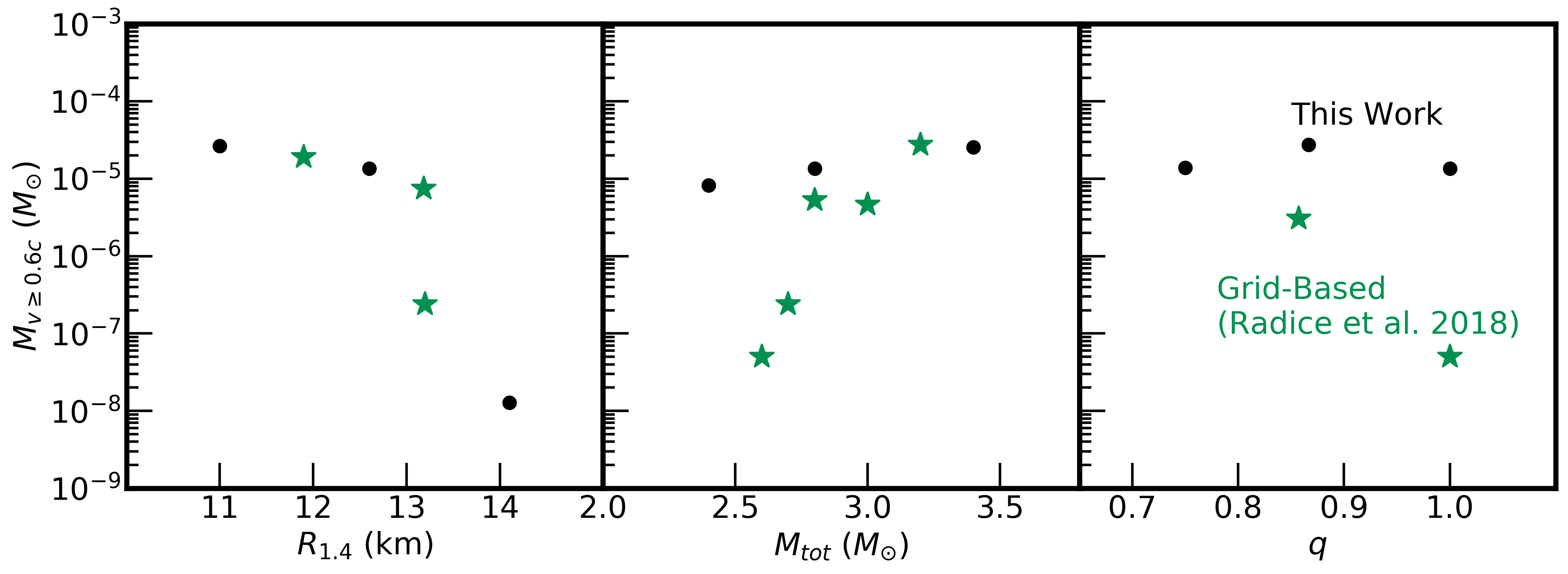
Figure 10: Total fast ejecta from our simulations (black circles), for varying EOS (left), total binary mass (center), and mass ratio (right). See Table LABEL:tab:models for model parameters. For comparison, green stars show a subset of the fast ejecta results from Radice et al. (2018) with the closest parameters. Note that Radice et al. (2018) also reports a merger with compactness that falls between the leftmost two data points in the left panel, which produces no fast ejecta (LS220_M135135_LK). Similarily, two runs by Radice et al. (2018) with total masses of $2.4$ and $2.5{M_{\odot}}$ (DD2_M120120_LK and DD2_M125125_LK) also produce no fast ejecta.

The angle-velocity mass histogram (Figure 11) shows that for the least compact model BPAL12, the high-velocity tail of the contact plane ejecta disappears, yielding a more uniform distribution in polar angle. The highest compactness model APR1 shows an extension of the contact plane ejecta to even higher velocities, and an increase in the amount of fast equatorial ejecta.

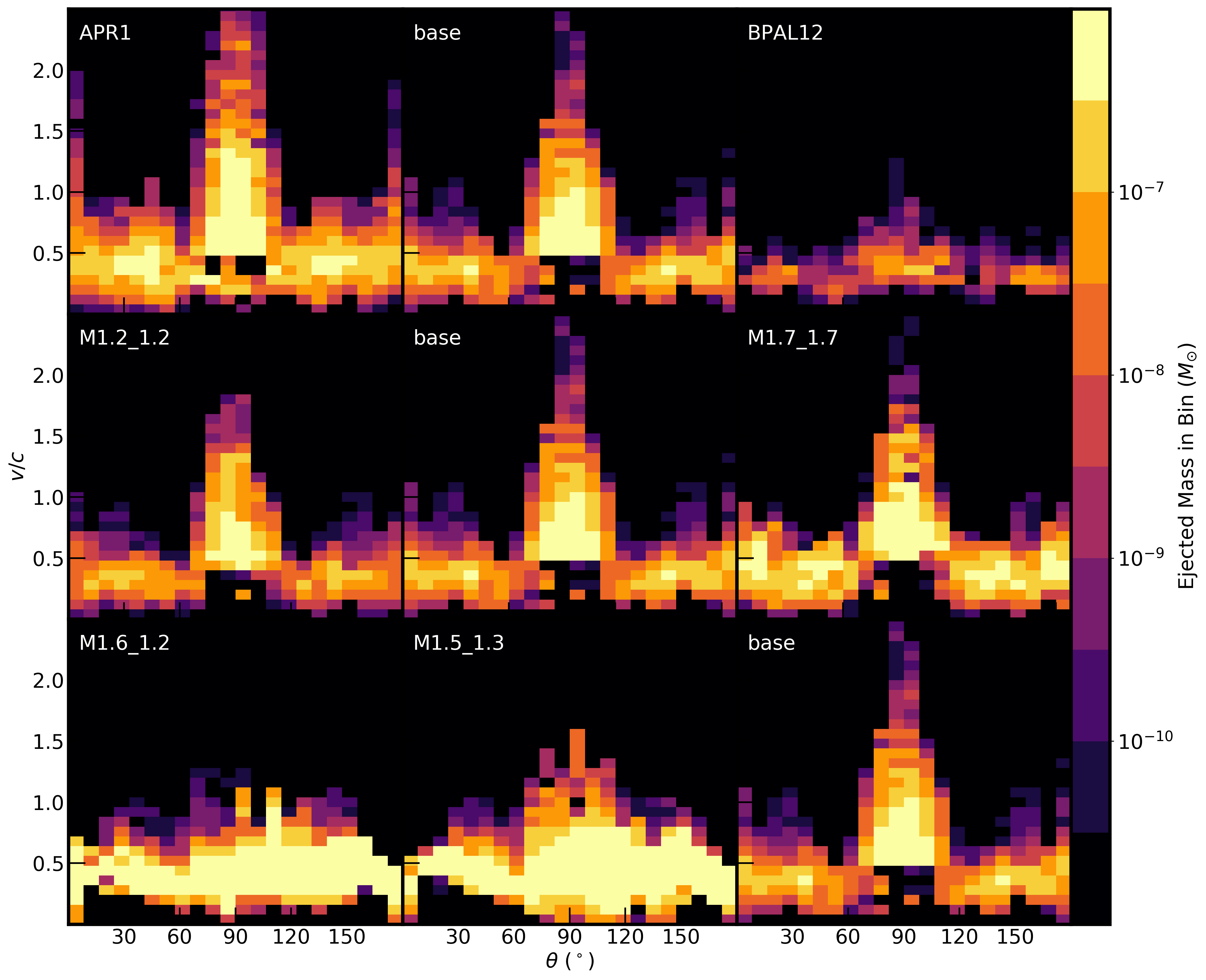
Figure 11: Same as Figure 7 but for models that vary the EOS (top row), total binary mass (middle row), and mass ratio (bottom row), as labeled (c.f. Table LABEL:tab:models).

When varying the total mass of the binary system, we find a mild monotonic dependence of fast ejecta with binary mass. Going from a $1.2+1.2M_{\odot}$ binary to $1.7+1.7M_{\odot}$, we find an increase by a factor $\sim 3$ of both fast and slow ejecta masses (Figure 10). Our models, being Newtonian, exclude the possibility of prompt BH formation, which is a likely outcome of the model with the highest total binary mass. Prompt BH formation is usually detrimental for mass ejection (e.g., Hotokezaka et al. 2013; Bauswein et al. 2013).

Table LABEL:tab:models shows that in all cases that vary the total mass, the fast orbital plane ejecta remains subdominant compared to that launched toward the contact plane. This is consistent with the angle-velocity mass histogram (Figure 11), which shows very similar results for all 3 cases that change the total binary mass. For fixed EOS, more massive NSs have smaller radii and therefore larger compactness, again yielding the known trend of higher mass ejection for collisions that reach deeper into the gravitational potential.

Changing the mass ratio at fixed constant binary mass yields a non-monotonic trend in fast ejecta production, with changes in total fast ejecta of a factor $\sim 2$ (Figure 10). By increasing the asymmetry of the binary, the number of ejection bursts increases from 2 bounces in the equal-mass base case to 4 or more oscillations for the asymmetric models (M1.5_1.3 and M1.6_1.2). Additionally, orbital plane ejecta is predominantly launched (factor $\sim 3$) in the direction of the smaller star.

Table LABEL:tab:models shows that the majority of fast ejecta continues to be produced toward the contact plane, with overall changes in this subset dominating the overall trend. An additional trend is a sharp increase in the amount of equatorial fast ejecta with decreasing mass ratio by a factor $30$ over the range explored. However, even in the most asymmetric case ($1.6+1.2M_{\odot}$), the equatorial plane contribution to the fast ejecta is lower by a factor $10$ than that from the contact plane. The angle-velocity histogram (Figure 11) shows that increasing the asymmetry of the binary results in a decrease of the high-velocity tail of the contact plane ejecta, and a more isotropic production of ejecta.

3.4 Discussion and Comparison with previous work

Our baseline configuration yields fast ejecta quantities that fall in between those found using SPH and grid-based methods, as shown in Figure 9. Given the number of approximations necessary to make our numerical experiment possible, the absolute amount of fast ejecta we find is not the most reliable quantity. Nonetheless, our most important result is that there is little resolution dependence in this fast ejecta when going from typical cell sizes employed in global 3D merger simulations using grid-based codes ($\sim 100$ m) to values that can capture the dynamics at the stellar surface reliably (few m).

We consider this resolution dependence to be a robust result, for the following reasons. First, the neutron stars and post-collision remnant are spatially extended on scales $\sim R_{\rm NS}$. The gravitational acceleration should be insensitive to small scale effects, except if a strong curvature develops. The latter can arise with prompt black hole formation, which is not considered in this study. Of particular concern would be high-mass binaries very close to prompt collapse, in which a change in spatial resolution could drastically change the amount of mass ejected. Second, mass ejected at high speeds becomes length-contracted in the laboratory frame. This effect becomes significant for relativistic momenta $\gamma\beta\gtrsim 1$. In both our numerical experiment (Figure 7) and in global 3D merger simulations, the ejecta has a mass distribution which is a decreasing function of velocity. We can estimate the error introduced by ignoring relativistic kinematics by computing the ratio of fast ejecta with $v>c$ to that with $v>0.6c$ in the base model: $M_{v\geq c}/M_{v\geq 0.6c}\simeq 0.17$. This $20\%$ uncertainty in our fast ejecta values due to the Newtonian description is comparable to the changes with grid spacing in our best resolved models. For comparison, Radice et al. (2018) finds variations of order a few in fast ejecta mass when increasing the resolution from $185$ m to $123$ m. Our models yield a similar resolution dependence when changing the grid spacing from $281$ m to $141$ m.

The choice of extraction radius at $30$ km does introduce a degree of uncertainty in the absolute values of fast ejecta that we report. Increasing this extraction radius to $90$ km decreases the fast ejecta mass by a factor $\sim 2$ in the base model. Most of this fast ejecta leaves the computational domain before the end of the simulation, therefore this dependence on the position of the extraction radius implies some degree of slowdown in the vicinity of the collision remnant. Since all simulations are measured with the same extraction radius, however, the position of this surface should not significantly affect changes in fast ejecta with resolution.

Our definition of fast ejecta ($v>0.6$ c) has been adopted to allow direct comparison with previous work. For the purposes of estimating the freezout of the $r$-process, however, a more strict criterion involves using the expansion time, with the relevant material expanding to densities $4\times 10^{5}$ g cm^-3 in less than $5$ ms (Metzger et al. 2015). For completeness, we estimate the expansion time of our fast ejecta material. In the absence of tracer particles, we compute this estimate as follows. We first consider the angle-averaged radial profile of the density of ejected material beyond the sampling radius at a time $t=0.49$ ms (Figure 12), with the average carried out over the contact plane for the base model, and over the orbital plane for model FF, since these directions contain the majority of the fast ejecta (Table LABEL:tab:models). Assuming the material ejection is in steady state, we estimate an upper limit to the expansion time for the base model as the crossing time from $30$ km to $60$ km at $v=0.6$ c, at which point the target density for freezout is reached. This yields an expansion time of $1.6\times 10^{-4}$ s. For the FF case, we extrapolate the density profile and find the distance necessary to reach the target density for freezout, and compute the crossing time at $v=0.6c$. The result is a slightly longer $5.8\times 10^{-4}$ s. In both cases, these simple estimates indicate that our velocity cut at $0.6$ c is more strict than what is needed to achieve neutron freezeout, with a corresponding underestimate of the mass available to power a precursor. Lowering the velocity cut in our numerical experiment would increase our “fast” ejecta at most by a factor of $\sim 2$, however, since our slow ejecta is of comparable magnitude (Table LABEL:tab:models). But since global 3D merger simulations produce significantly more slow ejecta, the exact value of the velocity cut can be in part responsible for the large discrepancy with particle-based results. The velocity distribution of ejecta in Figure 1 of Metzger et al. (2015) shows that there is indeed non-negligible free neutron production for $0.4<v/c<0.6$. A more careful analysis of this question requires use of sufficient tracer particles to sample the fraction of the velocity distribution that will yield the ejecta of interest.

Given the extraction radius dependence of our fast ejecta values, and the possibility that more free neutrons can be produced at $v<0.6c$, we can adopt a fiducial uncertainty of a factor $\sim 2$ in the absolute values of our fast ejecta.

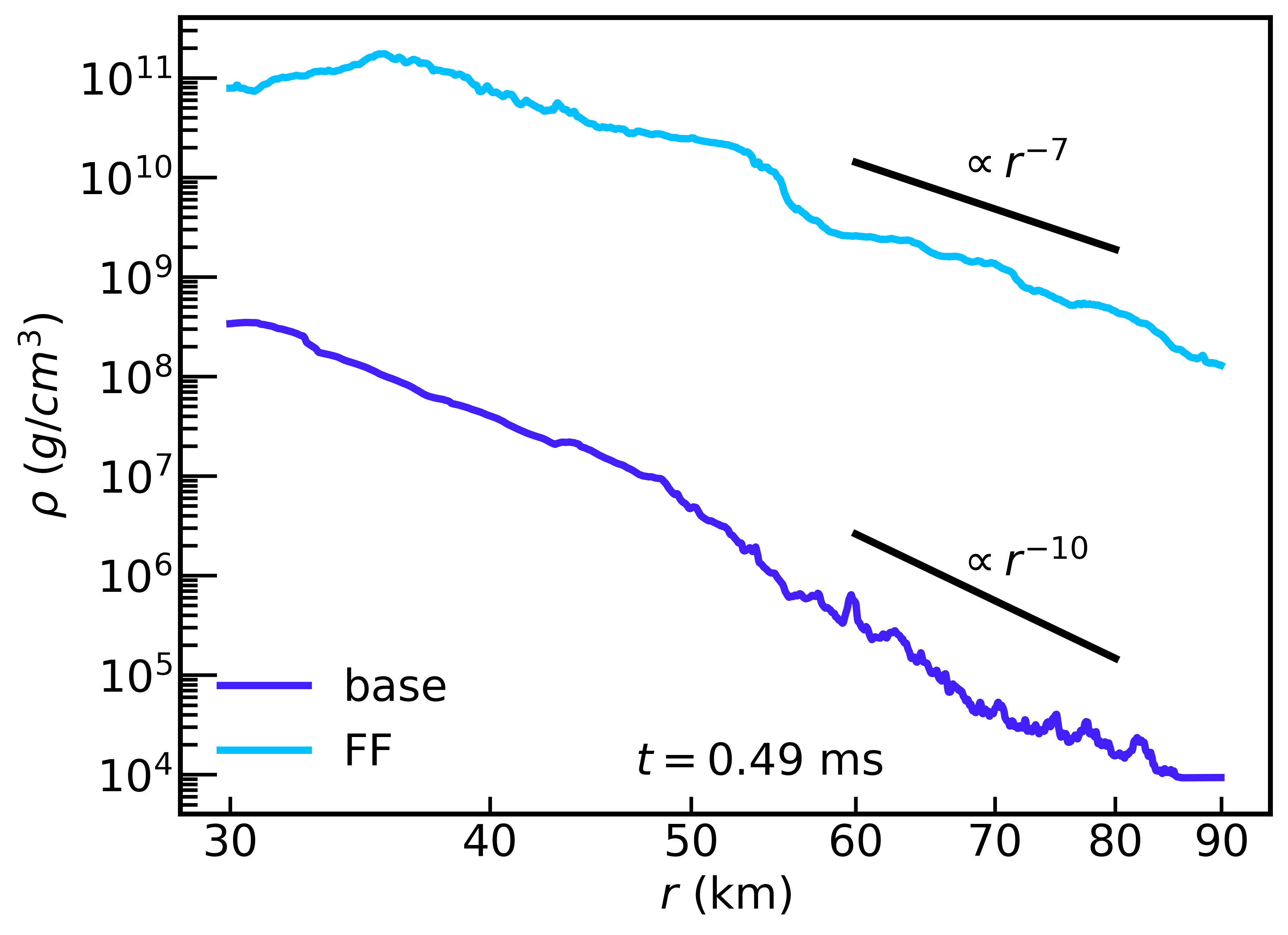
Figure 12: Angle-averaged radial profiles of density at $0.49$  ms for models base (purple) and FF (blue), with the average carried out over the contact and orbital plane directions, respectively. Radial slopes of $r^{-7}$ and $r^{-10}$ are shown for reference.

Since most of our simulations are only run long enough for production of fast ejecta to be complete, slow ejecta is still being produced by the end of the simulation. By the end of our base model, $2.5\times 10^{-5}{M_{\odot}}$ of total ejecta is produced. This is roughly an order of magnitude less ejecta than the closest case in Radice et al. (2018), and about two orders of magnitude less ejecta than was produced in the SPH simulation performed by Bauswein et al. (2013). While short run times (set by computational resources) are partly responsible for this lack of slow ejecta, our lower resolution models (R281, R141, R70) which run for ten times longer than the base case still do not produce sufficient slow ejecta to match 3D global simulations. For example, model R70 produces $1\%$ more fast ejecta and a factor of $\sim 2$ more slow ejecta for an increased runtime a factor of 10 longer. The imposition of axisymmetry and other approximations therefore also play a role in this discrepancy.

An important difference between our results and those of Radice et al. (2018) is the way in which most of the fast ejecta is produced, a likely consequence of the approximations made in our study. Radice et al. (2018) finds that fast ejecta emerges in two bursts, first from the contact interface and then from the first bounce of the HMNS remnant. The first burst is not always present, but the HMNS bounce is more robust and dominates the production of fast ejecta. We see a two burst structure in many of our simulations when varying total mass, or EOS (except in the low compactness case BPAL12, which produces less contact plane ejecta). This is also apparent in our force prescription variations, with FF producing an additional late time burst. This burst structure however is largely a temporal variation, with the majority of the ejecta in each burst being launched in the contact plane, whereas Radice et al. (2018) finds the first burst to be launched toward the contact plane, and the second burst being distinctly constrained to the orbital plane.

The direction of the trends of fast ejecta quantity with EOS and total mass in our models (Figure 10) compare favorably with those found by Radice et al. (2018), with our dependence on total mass being milder. Stronger differences are found when considering the mass ratio: Radice et al. (2018) obtains a strong monotonic dependence, whereas our models yield a non-monotonic trend with changes of a factor $\sim 2$ only. Changing the mass ratio does however result in a more broad angular distribution in our simulations, with a larger fraction of fast ejecta being launched in the orbital plane in more asymmetric binaries.

4 Implications for Kilonovae

4.1 Neutron-powered precursors

For a given quantity of forward fast ejecta $M_{\rm n}$ that freezes out the $r$-process, which here we take to be fast ejecta with $v\geq 0.6$ c, the peak bolometric luminosity of the ultraviolet precursor is given by (Metzger et al. 2015)

$$L_{\rm peak}=M_{\rm n}\dot{e}_{n}\lesssim 5\times 10^{42}\left(\frac{M_{\rm n}}{10^{-5}\,{M_{\odot}}}\right)\textrm{\,erg\,s}^{-1}$$ (19)

where

$$\dot{e}_{n}=3.2\times 10^{14}(1-2Y_{e})\textrm{\,erg\,s}^{-1}\,\textrm{g}^{-1}.$$ (20)

is the specific heating rate due to free neutron decay, and we have used an electron fraction $Y_{e}=0.1$ to estimate an upper limit for the free neutron mass fraction in evaluating equation (19). The corresponding time to peak emission is

$$t_{\rm peak}\simeq 0.3\,{\rm h\,}\left(\frac{M_{\rm n}}{10^{-5}\,{M_{\odot}}}\right)^{1/2}\left(\frac{\kappa}{1\,\textrm{cm}^{2}\,\textrm{g}^{-1}}\right)^{1/2}\left(\frac{v}{0.6\,\textrm{c}}\right)^{-1/2},$$ (21)

where $\kappa$ is the effective gray opacity of the ejecta, the value of which can vary in the range $1-30$ cm² g^-1 depending on the composition and ionization state of the ejecta (e.g., Tanaka et al. 2018). The fast ejecta produced in our baseline configuration, $M_{\rm n}\sim 10^{-5}\,M_{\odot}$ almost independent of spatial resolution, would correspond to the estimates above. Extrapolating the light curve models of Metzger et al. (2015) to lower neutron masses, one would predict that for $\sim 10^{-5}\,M_{\odot}$ of free neutrons, the precursor emission would peak around U-band (365 nm) at an AB magnitude $\approx 23$ for a source distance of $200$ Mpc. The planned wide-field ULTRASAT satellite mission (Sagiv et al. 2014) is expected to reach a 5$\sigma$ limiting magnitude of $\sim 23$ for a 1-hour integration at a wavelength of 220-280 nm. ULTRASAT observations of nearby mergers (¡ $200$ Mpc) could in principle probe the neutron precursor emission given this level of fast ejecta production.

When we consider our main result of a weak dependence of $M_{\rm n}$ on spatial resolution for grid-based simulations, and the normalization of this quantity obtained in the global 3D merger simulations of Radice et al. (2018) (e.g., Figure 10), we conclude that the neutron-powered precursor luminosities and timescales in equations (19)-(21) are likely to be an upper limit to luminosity and duration of this transient, at least as arising from the prompt dynamical ejecta. Other ways to produce fast ejecta include magnetically-accelerated, neutrino-heated winds from the magnetized neutron star remnant (Metzger et al. 2018; Ciolfi & Kalinani 2020), outflows from accretion disks with strong initial poloidal fields (Fernández et al. 2019), jet-cocoon interactions (Gottlieb & Loeb 2020), or ablation from an early neutrino burst generated from the colliding stellar interface (Beloborodov et al. 2020). More reliable estimates of the fast ejecta from the entire merger event will therefore require realistic initial conditions and a complete physics description, including MHD and neutrino transport effects.

The free-fall, head-on collision case yields $\sim 10^{-2}M_{\odot}$ of fast ejecta, with $\sim 10\%$ variation with spatial resolution. Once the time to peak becomes longer than the free neutron decay time, the luminosity estimate in equation (19) is no longer valid. Nevertheless, we expect this fact ejecta to contribute to the early kilonova signature, which should contain the imprint of much faster expansion velocities than those inferred from GW170817 and therefore provide a distinct signature of eccentric mergers.

4.2 Non-thermal afterglows

The dynamical ejecta is predicted to generate its own non-thermal afterglow after expanding sufficiently to interact with the interstellar medium on a timescale of years (Nakar & Piran 2011). The duration and brightness of the afterglow depend primarily on the kinetic energy distribution of the ejecta as well as on the interstellar medium density (e.g., Kathirgamaraju et al. 2019). Fast dynamical ejecta can produce an afterglow that evolves on shorter timescales of $\sim$ months (Hotokezaka et al. 2018), and such a fast component has been proposed as a possible origin of the X-ray excess recently detected in the non-thermal GW170817 emission (Hajela et al. 2021; Nedora et al. 2021).

Here we focus on the implications of our resolution study for the expected kilonova afterglows from BNSs. Given that our simulations are Newtonian, we cannot produce a reliable relativistic momentum distribution. Nevertheless, we can compute the kinetic energy of all the ejecta above a given velocity, and look at its resolution dependence.

Table LABEL:tab:models shows the kinetic energy of all the ejecta with radial velocities greater than $0.3$  and $0.6$ c. The first velocity was found by Kathirgamaraju et al. (2019) to be the minimum value needed to obtain a detectable afterglow. Our baseline configuration yields characteristic kinetic energies $\sim 10^{49}$ erg, a factor $100$ below what is needed to generate a detectable afterglow. This is likely a consequence of the underproduction of slow ejecta by our numerical experiment relative to global 3D merger simulations (§3.4), given that most of the kinetic energy normally resides in slower ejecta.

Despite this underproduction, we find that there is a convergence in the kinetic energy (above both velocities) to within $10\%$ for a resolution of $16$ m, similar to the convergence in mass. This is consistent with the estimates of Kyutoku et al. (2014) for the characteristic cell size at which shock breakout is properly resolved. We note however that, in contrast to the mass, relativistic material can carry a significant fraction of the total energy, hence the lack of relativistic kinematics makes our estimates of energy dependence on resolution only suggestive. Our results nevertheless indicate that robust predictions about the kilonova afterglow from the dynamical ejecta require higher spatial resolution than used to date in global 3D merger simulations.

5 Summary

We have carried out a numerical experiment to probe the sensitivity to spatial resolution of fast ejecta ($v>0.6$ c) generation in grid-code simulations of binary neutron star mergers. Discrepancies in the amount of this ejecta of an order of magnitude or larger have been found in global 3D merger simulations using grid codes compared to the amounts found in SPH simulations. We implement an axisymmetric model of stellar collision in a co-rotating frame, including the effects of inertial forces and gravitational wave losses (Section 2.1-2.2). The lower computational expense of this setup allow us to probe spatial resolutions up to $4$ m, or $\sim 3\times 10^{-4}$ of the neutron star radius, smaller than the finest grids used thus far in global 3D simulations of neutron star mergers by a factor of $\sim 20$, and capturing the surface pressure scale height of the stars above within $0.1\%$ of the stellar surface (Figure 3). Our main results are the following:

1. – Our baseline configuration of two $1.4M_{\odot}$ NSs with radius $12.6$ km ejects $\sim 10^{-5}M_{\odot}$ of fast ejecta, with variations in this quantity of at most a factor of $\sim 2$ over a factor $140$ in cell size, converging to within $10\%$ at a spatial resolution of $20$ m (Figure 9). While the absolute amount of ejecta is influenced by the approximations made in our reduced dimensionality experiment, the sensitivity to spatial resolution should be a robust outcome because of lack of strong curvature effects and a limited fraction of the ejecta moving at relativistic speeds that introduce significant length-contraction effects. We conclude that existing grid-based, global 3D hydrodynamic simulations of binary NS mergers (e.g., Radice et al. 2018) are close to converging in the amount of fast ejecta, and the known discrepancy with SPH simulations is unlikely to be caused by lack in resolution. A quantity of fast of ejecta of the order of $\sim 10^{-5}M_{\odot}$ is detectable with upcoming space-based UV facilities out to $\lesssim 200$ Mpc (Section 4).

2. – A head-on collision at the free-fall speed can eject $\sim 10^{-2}M_{\odot}$ of both fast and slow ejecta (Figure 5, Table LABEL:tab:models). For the case in which such a collision becomes possible due to a highly eccentric merger, the corresponding kilonova signature can be distinct from that arising in a more conventional quasi-circular merger driven by GW emission. When varying the resolution by a factor of $4$, we find that the total ejecta from our head-on collision models can vary non-monotonically at the $\sim 20\%$ level.

3. – Our numerical experiment reproduces the overall trends of fast ejecta generation with compactness (EOS) and total binary mass (Figure 10) when compared to the global 3D study of Radice et al. (2018). We find a non-monotonic dependence on mass ratio, which differs from that found previously. These differences can be attributed primarily to the approximations made in our experiment, particularly the reduced dimensionality and functional form of gravitational wave losses (Section 2.1-2.2). While we observe production of fast ejecta in bursts in our default configuration (Figure 6), the nature of these bursts is such that ejection is primarily in the contact plane direction, in contrast to the global simulations of Radice et al. (2018) in which the second, more robust burst is confined to the equatorial plane. Additionally, our models preclude the possibility of prompt BH formation, which can occur at high total binary masses and result in reduced ejecta production relative to what we find.

4. – The kinetic energy of the fast ejecta has a similar dependece on resolution than the mass. This suggests that predictions for the non-thermal kilonova afterglow require global 3D simulations with higher resolutions than those done thus far.

Four additional channels have been proposed for the production of fast ejecta: neutrino-driven outflows from magnetized neutron star remnants (Metzger et al. 2018; Ciolfi & Kalinani 2020), outflows from accretion disks with strong initial poloidal fields (Fernández et al. 2019), cocoon-jet interactions (Gottlieb & Loeb 2020), or ablation of stellar material by neutrinos (Beloborodov et al. 2020). A more realistic estimate of the total amount of fast ejecta produced in a binary neutron star merger thus requires (1) modeling the collision in general-relativistic MHD with adequate neutrino transport and with sufficient spatial resolution, and (2) use of realistic post-merger initial conditions in the case of fixed-metric codes are used. Such a calculation would provide useful information beyond the fast ejecta, and therefore is a valuable direction to pursue.

The head-on collision of neutron stars at the free-fall speed remains a simpler problem which, when done in numerical relativity and with sufficient spatial resolution, can yield useful predictions for the ejecta components from eccentric mergers, allowing an estimate of the electromagnetic signal and nucleosynthesis contributions from these collisions.

References

- Abbott et al. (2017a) Abbott, B. P., et al. 2017a, ApJ, 848, L12, doi: 10.3847/2041-8213/aa91c9
- Abbott et al. (2017b) —. 2017b, Nature, 551, 85, doi: 10.1038/nature24471
- Abbott et al. (2017c) —. 2017c, ApJ, 848, L13, doi: 10.3847/2041-8213/aa920c
- Abbott et al. (2018) —. 2018, Phys. Rev. Lett., 121, 161101, doi: 10.1103/PhysRevLett.121.161101
- Akmal et al. (1998) Akmal, A., Pandharipande, V. R., & Ravenhall, D. G. 1998, Phys. Rev. C, 58, 1804, doi: 10.1103/PhysRevC.58.1804
- Arcavi (2018) Arcavi, I. 2018, ApJ, 855, L23, doi: 10.3847/2041-8213/aab267
- Barnes & Kasen (2013) Barnes, J., & Kasen, D. 2013, ApJ, 775, 18, doi: 10.1088/0004-637X/775/1/18
- Bauswein et al. (2013) Bauswein, A., Goriely, S., & Janka, H. T. 2013, ApJ, 773, 78, doi: 10.1088/0004-637X/773/1/78
- Bauswein et al. (2010) Bauswein, A., Janka, H.-T., & Oechslin, R. 2010, PRD, 82, 084043, doi: 10.1103/PhysRevD.82.084043
- Beloborodov et al. (2020) Beloborodov, A. M., Lundman, C., & Levin, Y. 2020, ApJ, 897, 141, doi: 10.3847/1538-4357/ab86a0
- Blanchard et al. (2017) Blanchard, P. K., et al. 2017, ApJ, 848, L22, doi: 10.3847/2041-8213/aa9055
- Bovard et al. (2017) Bovard, L., Martin, D., Guercilena, F., et al. 2017, Phys. Rev. D, 96, 124005, doi: 10.1103/PhysRevD.96.124005
- Centrella & McMillan (1993) Centrella, J. M., & McMillan, S. L. W. 1993, ApJ, 416, 719, doi: 10.1086/173272
- Chaurasia et al. (2018) Chaurasia, S. V., Dietrich, T., Johnson-McDaniel, N. K., et al. 2018, Phys. Rev. D, 98, 104005, doi: 10.1103/PhysRevD.98.104005
- Childs et al. (2012) Childs, H., et al. 2012, in High Performance Visualization–Enabling Extreme-Scale Scientific Insight (eScholarship, University of California), 357–372. https://escholarship.org/uc/item/69r5m58v
- Ciolfi & Kalinani (2020) Ciolfi, R., & Kalinani, J. V. 2020, ApJ, 900, L35, doi: 10.3847/2041-8213/abb240
- Colella & Woodward (1984) Colella, P., & Woodward, P. R. 1984, JCP, 54, 174
- Couch et al. (2013) Couch, S. M., Graziani, C., & Flocke, N. 2013, ApJ, 778, 181, doi: 10.1088/0004-637X/778/2/181
- Cowperthwaite et al. (2017) Cowperthwaite, P. S., et al. 2017, ApJ, 848, L17, doi: 10.3847/2041-8213/aa8fc7
- Dietrich et al. (2017) Dietrich, T., Ujevic, M., Tichy, W., Bernuzzi, S., & Brügmann, B. 2017, Phys. Rev. D, 95, 024029, doi: 10.1103/PhysRevD.95.024029
- Douchin & Haensel (2001) Douchin, F., & Haensel, P. 2001, A&A, 380, 151, doi: 10.1051/0004-6361:20011402
- Drout et al. (2017) Drout, M. R., et al. 2017, Science, 358, 1570, doi: 10.1126/science.aaq0049
- Dubey et al. (2009) Dubey, A., Antypas, K., Ganapathy, M. K., et al. 2009, J. Par. Comp., 35, 512 , doi: DOI: 10.1016/j.parco.2009.08.001
- Fernández & Metzger (2016) Fernández, R., & Metzger, B. D. 2016, ARNPS, 66, 23, doi: 10.1146/annurev-nucl-102115-044819
- Fernández et al. (2019) Fernández, R., Tchekhovskoy, A., Quataert, E., Foucart, F., & Kasen, D. 2019, MNRAS, 482, 3373, doi: 10.1093/mnras/sty2932
- Fontes et al. (2015) Fontes, C. J., Fryer, C. L., Hungerford, A. L., et al. 2015, High Energy Density Physics, 16, 53, doi: 10.1016/j.hedp.2015.06.002
- Fryxell et al. (2000) Fryxell, B., Olson, K., Ricker, P., et al. 2000, ApJS, 131, 273, doi: 10.1086/317361
- Gold et al. (2012) Gold, R., Bernuzzi, S., Thierfelder, M., Brügmann, B., & Pretorius, F. 2012, Phys. Rev. D, 86, 121501, doi: 10.1103/PhysRevD.86.121501
- Goriely et al. (2014) Goriely, S., Bauswein, A., Janka, H. T., et al. 2014, in American Institute of Physics Conference Series, Vol. 1594, American Institute of Physics Conference Series, ed. S. Jeong, N. Imai, H. Miyatake, & T. Kajino, 357–364, doi: 10.1063/1.4874095
- Gottlieb & Loeb (2020) Gottlieb, O., & Loeb, A. 2020, MNRAS, 493, 1753, doi: 10.1093/mnras/staa363
- Hajela et al. (2021) Hajela, A., Margutti, R., Bright, J. S., et al. 2021, arXiv e-prints, arXiv:2104.02070. https://arxiv.org/abs/2104.02070
- Harris et al. (2020) Harris, C. R., et al. 2020, Nature, 585, 357, doi: 10.1038/s41586-020-2649-2
- Hotokezaka et al. (2013) Hotokezaka, K., Kiuchi, K., Kyutoku, K., et al. 2013, Phys. Rev. D, 87, 024001, doi: 10.1103/PhysRevD.87.024001
- Hotokezaka et al. (2018) Hotokezaka, K., Kiuchi, K., Shibata, M., Nakar, E., & Piran, T. 2018, ApJ, 867, 95, doi: 10.3847/1538-4357/aadf92
- Hunter (2007) Hunter, J. D. 2007, Computing In Science & Engineering, 9, 90, doi: 10.1109/MCSE.2007.55
- Ishii et al. (2018) Ishii, A., Shigeyama, T., & Tanaka, M. 2018, ApJ, 861, 25, doi: 10.3847/1538-4357/aac385
- Just et al. (2015) Just, O., Bauswein, A., Ardevol Pulpillo, R., Goriely, S., & Janka, H. T. 2015, MNRAS, 448, 541, doi: 10.1093/mnras/stv009
- Kasen et al. (2013) Kasen, D., Badnell, N. R., & Barnes, J. 2013, ApJ, 774, 25, doi: 10.1088/0004-637X/774/1/25
- Kathirgamaraju et al. (2019) Kathirgamaraju, A., Giannios, D., & Beniamini, P. 2019, MNRAS, 487, 3914, doi: 10.1093/mnras/stz1564
- Kellerman et al. (2010) Kellerman, T., Rezzolla, L., & Radice, D. 2010, Classical and Quantum Gravity, 27, 235016, doi: 10.1088/0264-9381/27/23/235016
- Kiuchi et al. (2017) Kiuchi, K., Kawaguchi, K., Kyutoku, K., et al. 2017, PRD, 96, 084060, doi: 10.1103/PhysRevD.96.084060
- Kulkarni (2005) Kulkarni, S. R. 2005, preprint, astro-ph/0510256. https://arxiv.org/abs/astro-ph/0510256
- Kyutoku et al. (2014) Kyutoku, K., Ioka, K., & Shibata, M. 2014, MNRAS, 437, L6, doi: 10.1093/mnrasl/slt128
- Lehner et al. (2016) Lehner, L., Liebling, S. L., Palenzuela, C., et al. 2016, Classical and Quantum Gravity, 33, 184002, doi: 10.1088/0264-9381/33/18/184002
- Levan et al. (2017) Levan, A. J., et al. 2017, ApJ, 848, L28, doi: 10.3847/2041-8213/aa905f
- Li & Paczyński (1998) Li, L.-X., & Paczyński, B. 1998, ApJ, 507, L59, doi: 10.1086/311680
- Lippuner et al. (2017) Lippuner, J., Fernández, R., Roberts, L. F., et al. 2017, MNRAS, 472, 904, doi: 10.1093/mnras/stx1987
- Loken et al. (2010) Loken, C., et al. 2010, Journal of Physics: Conference Series, 256, 012026, doi: 10.1088/1742-6596/256/1/012026
- Martin et al. (2015) Martin, D., Perego, A., Arcones, A., et al. 2015, ApJ, 813, 2, doi: 10.1088/0004-637X/813/1/2
- Metzger et al. (2015) Metzger, B. D., Bauswein, A., Goriely, S., & Kasen, D. 2015, MNRAS, 446, 1115, doi: 10.1093/mnras/stu2225
- Metzger et al. (2018) Metzger, B. D., Thompson, T. A., & Quataert, E. 2018, ApJ, 856, 101, doi: 10.3847/1538-4357/aab095
- Metzger et al. (2010) Metzger, B. D., Martínez-Pinedo, G., Darbha, S., et al. 2010, MNRAS, 406, 2650, doi: 10.1111/j.1365-2966.2010.16864.x
- Nakar & Piran (2011) Nakar, E., & Piran, T. 2011, Nature, 478, 82, doi: 10.1038/nature10365
- Nedora et al. (2021) Nedora, V., Radice, D., Bernuzzi, S., et al. 2021, arXiv e-prints, arXiv:2104.04537. https://arxiv.org/abs/2104.04537
- Papenfort et al. (2018) Papenfort, L. J., Gold, R., & Rezzolla, L. 2018, Phys. Rev. D, 98, 104028, doi: 10.1103/PhysRevD.98.104028
- Peters (1964) Peters, P. C. 1964, PhD thesis, California Institute of Technology
- Ponce et al. (2019) Ponce, M., et al. 2019, in Proceedings of the Practice and Experience in Advanced Research Computing on Rise of the Machines (Learning), PEARC ’19 (New York, NY, USA: Association for Computing Machinery), doi: 10.1145/3332186.3332195
- Porter & Woodward (1994) Porter, D. H., & Woodward, P. R. 1994, ApJS, 93, 309, doi: 10.1086/192057
- Radice et al. (2018) Radice, D., Perego, A., Hotokezaka, K., et al. 2018, ApJ, 869, 130, doi: 10.3847/1538-4357/aaf054
- Rasio & Shapiro (1992) Rasio, F. A., & Shapiro, S. L. 1992, ApJ, 401, 226, doi: 10.1086/172055
- Read et al. (2009) Read, J. S., Lackey, B. D., Owen, B. J., & Friedman, J. L. 2009, PRD, 79, 124032, doi: 10.1103/PhysRevD.79.124032
- Roberts et al. (2017) Roberts, L. F., Lippuner, J., Duez, M. D., et al. 2017, MNRAS, 464, 3907, doi: 10.1093/mnras/stw2622
- Rosswog (2013) Rosswog, S. 2013, Philosophical Transactions of the Royal Society of London Series A, 371, 20120272, doi: 10.1098/rsta.2012.0272
- Ruffert & Janka (1998) Ruffert, M., & Janka, H. T. 1998, A&A, 338, 535. https://arxiv.org/abs/astro-ph/9804132
- Sagiv et al. (2014) Sagiv, I., Gal-Yam, A., Ofek, E. O., et al. 2014, AJ, 147, 79, doi: 10.1088/0004-6256/147/4/79
- Sekiguchi et al. (2016) Sekiguchi, Y., Kiuchi, K., Kyutoku, K., Shibata, M., & Taniguchi, K. 2016, Phys. Rev. D, 93, 124046, doi: 10.1103/PhysRevD.93.124046
- Shapiro (1980) Shapiro, S. L. 1980, ApJ, 240, 246, doi: 10.1086/158229
- Tanaka & Hotokezaka (2013) Tanaka, M., & Hotokezaka, K. 2013, ApJ, 775, 113, doi: 10.1088/0004-637X/775/2/113
- Tanaka et al. (2017) Tanaka, M., et al. 2017, PASJ, 69, 102, doi: 10.1093/pasj/psx121
- Tanaka et al. (2018) Tanaka, M., Kato, D., Gaigalas, G., et al. 2018, ApJ, 852, 109, doi: 10.3847/1538-4357/aaa0cb
- Tanvir et al. (2017) Tanvir, N. R., et al. 2017, ApJ, 848, L27, doi: 10.3847/2041-8213/aa90b6
- Wanajo et al. (2014) Wanajo, S., Sekiguchi, Y., Nishimura, N., et al. 2014, ApJ, 789, L39, doi: 10.1088/2041-8205/789/2/L39
- Wu et al. (2016) Wu, M.-R., Fernández, R., Martínez-Pinedo, G., & Metzger, B. D. 2016, MNRAS, 463, 2323, doi: 10.1093/mnras/stw2156
- Zuo et al. (1999) Zuo, W., Bombaci, I., & Lombardo, U. 1999, Phys. Rev. C, 60, 024605, doi: 10.1103/PhysRevC.60.024605