Assessing diffusion model impacts on enstrophy and flame structure in turbulent lean premixed flames

Abstract

Diffusive transport of mass occurs at small scales in turbulent premixed flames. As a result, multicomponent mass diffusion, which is often neglected in direct numerical simulations (DNS) of premixed combustion, has the potential to impact both turbulence and flame characteristics at small scales. In this study, we evaluate these impacts by examining enstrophy dynamics and the internal structure of the flame for lean premixed hydrogen-air combustion, neglecting secondary Soret and Dufour effects. We performed three-dimensional DNS of these flames by implementing the Stefan–Maxwell equations in the code NGA to represent multicomponent mass transport, and we simulated statistically planar lean premixed hydrogen-air flames using both mixture-averaged and multicomponent models. The mixture-averaged model underpredicts the peak enstrophy in the multicomponent simulation by up to $13\text{\,}\mathrm{\char 37\relax}\text{/}$ in the flame front. Comparing the enstrophy budgets of these flames, the multicomponent simulation yields larger peak magnitudes compared to the mixture-averaged simulation in the reaction zone, showing differences of $17\text{\,}\mathrm{\char 37\relax}\text{/}$ and $14\text{\,}\mathrm{\char 37\relax}\text{/}$ in the normalized vortex stretching and viscous effects terms. In the super-adiabatic regions of the flame, the mixture-averaged model overpredicts the viscous effects by up to $13\text{\,}\mathrm{\char 37\relax}\text{/}$. To assess the effect of these differences on flame structure, we reconstructed the average local internal structure of the turbulent flame through statistical analysis of the scalar gradient field. Based on this analysis, we show that large differences in viscous effects contribute to significant differences in the average local flame structure between the two models.

1 Introduction

The average internal flame structure and statistical behavior of vorticity and enstrophy are critical for evaluating the properties and effects of turbulent fluid motions in reacting flows [1, 2, 3]. Both chemical heat release and advective mixing by turbulence can form steep gradients in temperature and scalar fields, increasing the importance of diffusive transport relative to effects due to chemical reactions in the flame dynamics [4]. Prior studies have shown that these enhanced diffusive effects are especially important in lean hydrogen flames where the Lewis number is much less than unity, leading to an increase in the turbulent flame speed [5]. A number of computational studies have also examined turbulent premixed flame characteristics for lean and low Lewis-number conditions [6, 7, 2, 8, 9]. Day et al. [6], in particular, showed that the effects of thermo-diffusive instabilities remain evident even in turbulent premixed flames where velocity fluctuations are nearly three times larger than the laminar flame speed, although stronger turbulence moderates the growth of cellular structures associated with these instabilities.

Several studies have already examined the importance of thermal diffusion in a wide range of flame configurations [10, 11, 12, 13, 6, 14, 7, 15, 16, 8, 9]. These studies have thoroughly demonstrated that neglecting thermal diffusion, in particular, can significantly impact flame properties. For example, studying three-dimensional (3D), premixed, turbulent hydrogen/air flames, Schlup and Blanquart [9] showed that thermal diffusion can increase flame propagation speeds and chemical source terms of products in regions of high positive curvature. For laminar hydrogen/air flames, Giovangigli [16] demonstrated that multicomponent Soret effects can significantly influence laminar flame speeds and extinction stretch rates for flat and stretched premixed flames, respectively. Based on these and other studies, thermal diffusion is thus important for understanding and accurately predicting the dynamics of some fuel/air mixtures.

Although several of the studies noted above have also evaluated the impact of multicomponent thermal diffusion models on lean hydrogen flame simulations [11, 12, 17, 18, 9], there is still an incomplete understanding of the impact of full multicomponent mass diffusion, a component of the exact scalar (e.g., chemical species concentration or mass fraction) governing equations, on turbulent transport and average flame structure. In many simulation studies of premixed flames, mass diffusion is represented using a mixture-averaged approximation, but this may significantly impact the coupled dynamics of scalars and turbulence, particularly in lean premixed hydrogen flames where thermo-diffusive instabilities are prominent. Recently, Fillo et al. [19] studied premixed, turbulent, high Karlovitz-number hydrogen/air, n-heptane/air, and toluene/air flames, showing that using the mixture-averaged diffusion model noticeably alters diffusion fluxes compared with the multicomponent diffusion model. These variations lead to differences of $520\text{\,}\mathrm{\char 37\relax}\text{/}$ in normalized turbulent flame speeds and conditional means of fuel source term. These observations motivate this deeper dive into the impacts of mass diffusion model on turbulence and flame dynamics.

The primary objective of this study is to evaluate the impact of the mixture-averaged diffusion approximation on enstrophy transport and the average internal flame structure using data from direct numerical simulations (DNS) of turbulent, premixed, lean hydrogen/air flames. This objective will be achieved in two ways. First, we will analyze the differences in time- and spatially averaged enstrophy budgets in the DNS using mixture-averaged and multicomponent diffusion models. Second, we will evaluate the impact of these differences on the average local flame structure by evaluating scalar gradient trajectories for the two models and statistically reconstructing the internal flame structures. Based on the results of these analyses, we will assess the accuracy and appropriateness of the mixture-averaged diffusion approximation for use in DNS of turbulent, premixed, lean hydrogen/air flames.

The paper is organized as follows. Section 2 describes the governing equations, diffusion models, and flow configuration for the 3D DNS. Then, Section 3 presents a qualitative description of the scalar and vorticity magnitude fields, the time- and spatially averaged enstrophy budgets, and the statistical reconstruction of the average turbulent flame width. Finally, in Section 4 we draw conclusions from the comparisons of the diffusion models.

2 Numerical approach

This section describes the governing reacting-flow equations, including brief discussions of the diffusion models to be studied. We also describe the 3D flow configuration modeled in the simulations.

2.1 Governing equations

The variable-density, low Mach number, reacting-flow equations are solved using the finite-difference code NGA [20, 21]. The conservation equations are written as rCl ∂ρ∂t+∇⋅(ρu) &= 0  ,
∂(ρu)∂t+∇⋅(ρu⊗u) = -∇p+∇⋅τ+f  ,
∂(ρT)∂t+∇⋅(ρu T) = ∇⋅( ρα∇T ) - 1cp∑_i c_p,ij_i ⋅∇T + ρ˙ω_T + ραcp ∇c_p ⋅∇T  ,
∂(ρYi)∂t+∇⋅(ρu Y_i) = -∇⋅j_i+ρ˙ω_i  , where $\rho$ is the mixture density, $\bm{u}$ is the velocity, $p$ is the hydrodynamic pressure, $\bm{\tau}$ is the viscous stress tensor, $\bm{f}$ represents volumetric forces, $T$ is the temperature, $\alpha$ is the mixture thermal diffusivity, $c_{p,i}$ is the constant-pressure specific heat of species $i$, $c_{p}$ is the constant-pressure specific heat of the mixture, and $\bm{j}_{i}$, $Y_{i}$ , and $\dot{\omega_{i}}$ are the diffusion flux, mass fraction, and production rate of species $i$, respectively. In Eq. (2.1), the temperature source term is given by

$$\dot{\omega}_{T}=-c_{p}^{-1}\sum_{i}h_{i}(T)\dot{\omega_{i}}\;,$$ (1)

where $h_{i}(T)$ is the specific enthalpy of species $i$ as a function of temperature. The density is determined from the ideal gas equation of state.

2.2 Overview of diffusion models

The diffusion fluxes are calculated using the semi-implicit scheme developed by Fillo et al. [22] with either the mixture-averaged [23, 4] or multicomponent [24] model, both of which are based on Boltzmann’s equation for the kinetic theory of gases [23, 24]. We neglect both baro-diffusion and thermal diffusion (i.e., Soret and Dufour effects). The baro-diffusion term is commonly neglected in reacting-flow simulations under the low-Mach-number approximation [25], and we neglected thermal diffusion because our objective is to investigate the impact of mass diffusion models only; Schlup and Blanquart [9] previously explored the effects of thermal diffusion models on lean premixed flames.

The species diffusion flux for the mixture-averaged diffusion model, denoted $\bm{j}_{i}^{\text{MA}}$, is related to the species gradient by a Fickian formulation and is expressed as

$$\bm{j}_{i}^{\text{MA}}=-\rho D_{i,m}\frac{Y_{i}}{X_{i}}\nabla X_{i}+\rho Y_{i}\bm{u}_{c}\;,$$ (2)

where $X_{i}$ is the $i$th species mole fraction and $D_{i,m}$ is the $i$th species mixture-averaged diffusion coefficient. This was originally introduced by Curtiss and Hirschfelder [23] and is expressed by Bird et al. [4] as

$$D_{i,m}=\frac{1-Y_{i}}{\sum_{i\neq j}^{N}X_{j}/\mathcal{D}_{ji}}\;.$$ (3)

Here $\mathcal{D}_{ji}$ is the binary diffusion coefficient for species $i$ and $j$, and $\bm{u}_{c}$ is the correction velocity used to ensure mass continuity:

$$\bm{u}_{c}=\sum_{i}D_{i,m}\frac{Y_{i}}{X_{i}}\nabla X_{i}\;.$$ (4)

While the mixture-averaged diffusion coefficient and correction velocity were introduced empirically, Giovangigli [27] showed that the resulting diffusion flux corresponds to the first term of a series converging towards the exact solution of the Stefan–Maxwell equations.

The species diffusion flux for the multicomponent diffusion model, denoted $\bm{j}_{i}^{\text{MC}}$, as presented by Bird et al. [4] and implemented in CHEMKIN II [28], is

$$\bm{j}_{i}^{\text{MC}}=\frac{\rho Y_{i}}{X_{i}W}\sum_{i\neq j}^{N}W_{j}D_{i,j}\nabla{X_{j}}\;,$$ (5)

where $W$ is the mixture molecular weight, $W_{j}$ is the molecular weight of the $j$th species, and $D_{i,j}$ is the multicomponent diffusion coefficient computed using the MCMDIF subroutine of CHEMKIN II [28] with the method outlined by Dixon-Lewis [29].

Table 1: Parameters describing the mixture-averaged (MA) and multicomponent (MC) diffusion simulations, with definitions provided, where $u^{\prime}$ is the turbulent fluctuating velocity, $\epsilon$ is the turbulent energy dissipation rate, and $\nu_{\text{u}}$ is the unburnt kinematic viscosity.

	MA	MC	Description
Domain	$8L\times L\times L$		Dimensions of the computational domain
$L$	190$\Delta{x}$		Spanwise width of the computational domain
Grid	$1520\times 190\times 190$		Computational grid size
$\Delta{x}$ [$\mathrm{mm}\text{/}$]	0.0424		Computational grid spacing
$\eta_{\text{u}}$ [$\mathrm{m}\text{/}$]	$2.1\text{\times}{10}^{-5}$		Kolmogorov length scale in the unburnt gas
$\tau_{\eta}$ [$\mathrm{s}\text{/}$]	$1.87\text{\times}{10}^{-5}$		Kolmogorov time scale in the unburnt gas
$\Delta{t}$ [$\mathrm{s}\text{/}$]	$6\text{\times}{10}^{-7}$		Simulation time-step size
$\phi$	0.4		Equivalence ratio
$P_{0}$ [$\mathrm{atm}\text{/}$]	$1$		Pressure of the unburnt mixture
$T_{\text{u}}$ [$\mathrm{K}\text{/}$]	$298$		Temperature of the unburnt mixture
$T_{\text{peak}}$ [$\mathrm{K}\text{/}$]	1190	1180	Temperature of peak fuel consumption rate in a laminar flame
$T_{\text{b}}$ [$\mathrm{K}\text{/}$]	1422	1422	Temperature of the burnt mixture in a laminar flame
$S_{L}$ [$\mathrm{m}\text{/}\mathrm{s}$]	0.230	0.223	Laminar flame speed
$\delta_{L}$ [$\mathrm{mm}\text{/}$]	0.643	0.631	Laminar flame thermal thickness $\delta_{L}=\left(T_{\text{b}}-T_{\text{u}}\right)/\left|\nabla T\right|_{\max}$
$\tau_{L}$ [$\mathrm{s}\text{/}$]	$2.80\text{\times}{10}^{-3}$	$2.83\text{\times}{10}^{-3}$	Laminar flame characteristic time scale $\tau_{L}=\delta_{L}/S_{L}$
$\ell/\delta_{L}$	2.00	2.04	Integral length scale $\ell=u^{\prime 3}/\epsilon$ relative to $\delta_{L}$
$u^{\prime}/S_{L}$	18.0	18.6	Turbulent fluctuation velocity relative to $S_{L}$
$\text{Ka}_{\text{u}}$	149	151	Karlovitz number in the unburnt mixture, $\text{Ka}_{\text{u}}=\tau_{L}/\tau_{\eta}$
$\text{Re}_{\text{t}}$	289		Reynolds number in the unburnt mixture, $\text{Re}_{\text{t}}=(u^{\prime}l)/\nu_{\text{u}}$

2.3 Simulation configuration

The simulations model a 3D statistically stationary, statistically planar lean premixed hydrogen/air flame [30, 31, 9]. This fuel/air mixture has a low Lewis number ($\mathrm{Le}_{\rm H_{2}}=0.3$) and was selected because the fidelity of the diffusion model (i.e., mixture-averaged or multicomponent) may be important for accurately simulating the instabilities associated with differential diffusion in lean hydrogen/air flames. Chemical reactions in the hydrogen/air mixture are represented using the nine-species, 54-reaction chemistry model from Hong et al. [32, 33, 34] (forward and backward reactions are counted separately).

The 3D turbulent flames are simulated using an identical flow configuration as in previous studies [35, 30, 9, 22, 19], and therefore we only briefly describe them here. The computational domain consists of inflow and convective outflow boundary conditions in the stream-wise (i.e., $x$) direction. The two span-wise directions (i.e., $y$ and $z$) use periodic boundaries. The inflow velocity is the mean turbulent flame speed, which keeps the flame statistically stationary such that turbulent statistics can be collected over an arbitrarily long run time. In the absence of mean shear, a linear turbulence forcing method [36, 37] is implemented to maintain the production of turbulent kinetic energy through the flame. Klein et al. [38] showed that, in statistically planar flame configurations such as those examined here, neither unforced decaying turbulence, boundary-only forcing, or linear forcing are clearly preferable, indicating that the linear forcing used here is sufficient for examining the relative impacts of different diffusion models in the present simulations.

Table 1 provides further details of the computational domain, unburnt mixture, corresponding one-dimensional flame statistics, and inlet turbulence in both the mixture-averaged (MA) and multicomponent (MC) diffusion simulations. The unburnt temperatures and pressures are $298\text{\,}\mathrm{K}\text{/}$ and $1\text{\,}\mathrm{atm}\text{/}$, respectively. The definitions of the unburnt Karlovitz number, $\text{Ka}_{\text{u}}$, and turbulent Reynolds number, $\text{Re}_{\text{t}}$, are also given in Table 1, where $\tau_{L}=\delta_{L}/S_{L}$ is the flame time scale and $\tau_{\eta}=\left(\nu_{\text{u}}/\epsilon\right)^{1/2}$ is the Kolmogorov time scale of the incoming turbulence. The forcing was designed to produce a turbulence integral scale $\ell=u^{\prime 3}/\varepsilon$ of roughly $2\delta_{L}$; directly calculating the integral scale from the longitudinal velocity correlation after the simulations were performed yields $\ell\approx 2.3\delta_{L}$, close to the intended integral scale. Based on this computed integral scale, the position of the flame in the simulation domain is roughly $8\ell$ from the inlet at $x/L=0$, suggesting that results in the flame region should not be strongly affected by the inlet boundary condition. We modeled relatively high Karlovitz numbers of $\mathrm{Ka}_{\text{u}}\approx 150$ in both simulations to represent cases where the turbulence timescale is shorter than the species diffusion timescale, resulting in pronounced impacts of the turbulence on the flame.

3 Results and discussion

In this section, we first present a qualitative description of the instantaneous velocity and scalar fields. Next, we present a time- and spatially averaged assessment of the enstrophy budget, followed by a statistical reconstruction of the average local flame structure.

3.1 Qualitative description

As an initial assessment of impact of mixture-averaged and multicomponent mass diffusion on flame dynamics, we present instantaneous flow fields for the simulated flames. Both simulations are initialized with the same scalar and velocity fields, and run for a single time iteration to evaluate the impact of diffusion on the scalar field, independent of turbulent mixing.

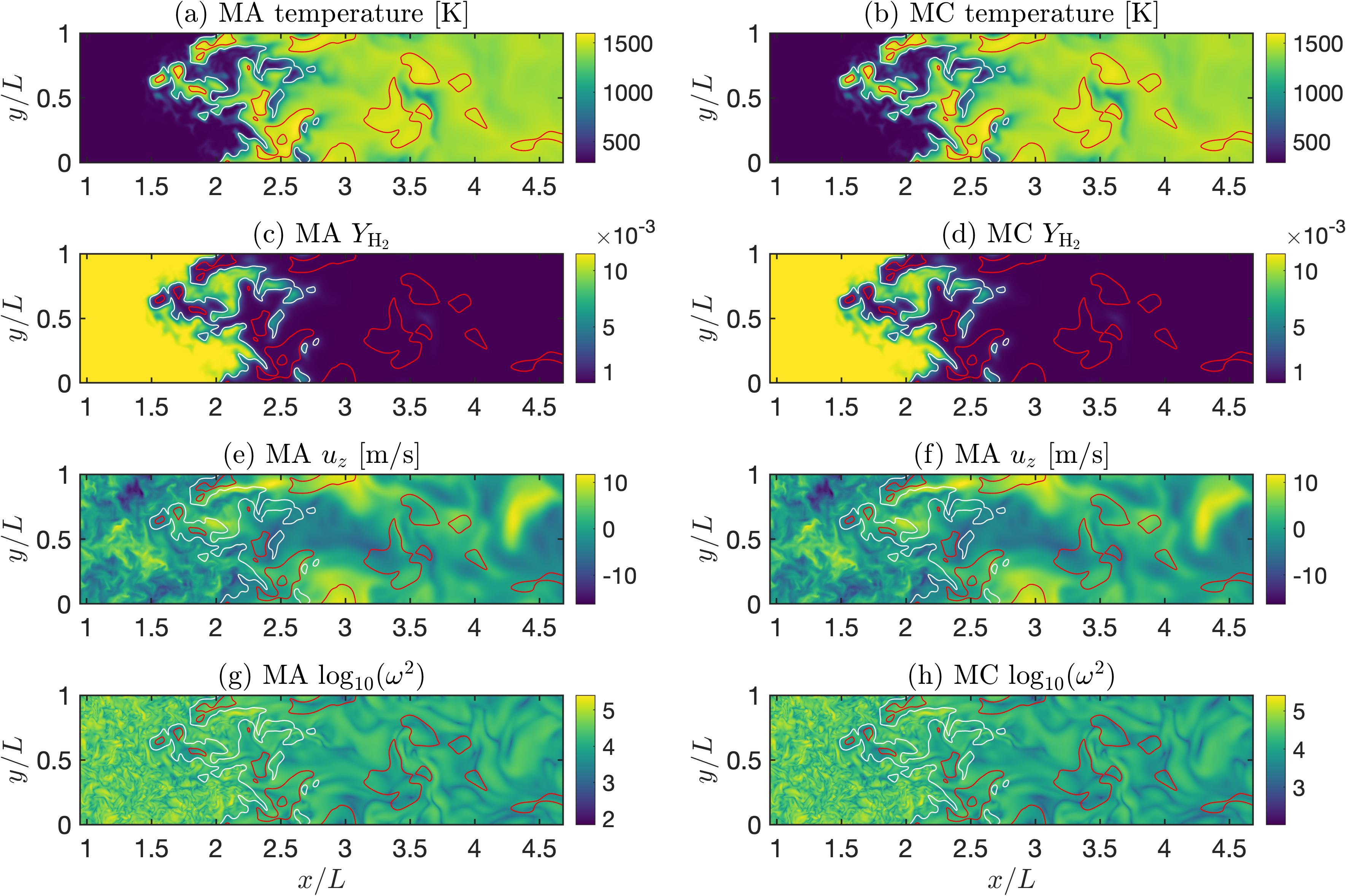
Figure 1: Instantaneous fields of temperature $T$ (a, b), fuel mass fraction $Y_{\text{H}_{2}}$ (c, d), $z$-direction velocity $u_{z}$ (e, f), and vorticity magnitude $\omega^{2}$ (g, h) for one time step of the hydrogen/air turbulent premixed flame for the mixture-averaged (MA) and multicomponent (MC) diffusion cases. Shown are domain cross-sections through the midplane. The red and white lines correspond to isosurfaces of $T_{0}=T_{\text{peak}}-$300\text{\,}\mathrm{K}\text{/}$$ and $T_{f}=T_{\text{peak}}+$300\text{\,}\mathrm{K}\text{/}$$, respectively, and represent the inflow and outflow surfaces of the flame front.

Figure 1 shows contours of temperature, hydrogen mass fraction, $z$-direction velocity, and the logarithm of the total vorticity magnitude ( $\omega=(\bm{\omega}\cdot\bm{\omega})^{1/2}$), where $\bm{\omega}=\nabla\times\bm{u}$. The inlet and outlet of the flame front are defined by the isosurfaces, $T_{0}=T_{\text{peak}}-$300\text{\,}\mathrm{K}\text{/}$$ and $T_{f}=T_{\text{peak}}+$300\text{\,}\mathrm{K}\text{/}$$, respectively, where $T_{\text{peak}}$ is the temperature of peak fuel consumption rate in the one-dimensional laminar flame (see Table 1). Figures 1(a,b) and (c,d) show that temperature increases across the flame as the fuel is consumed in both simulation cases. Figures 1(e,f) show that the velocity fields $u_{z}$ become smoother with fewer small-scale features across the flame, corresponding to an overall reduction in the vorticity magnitude from reactants to products, as Figs. 1(g,h) show.

Shown qualitatively in Fig. 1, the $T_{f}$ isosurface is located at the approximate transition point between the preheat and reaction zones, while the $T_{0}$ isosurface captures the super-adiabatic regions, also called “hot spots”, present in lean premixed hydrogen flames. These hot spots result from differential diffusion and have been predicted by theory [39] and shown in simulations of lean, premixed hydrogen/air flames, including in the post-flame region [6, 7, 40, 8]. Fillo et al. [19] previously showed that the two diffusion models result in differences of $535\text{\,}\mathrm{\char 37\relax}\text{/}$ in conditional means of both fuel mass fraction and source term in these hot spots.

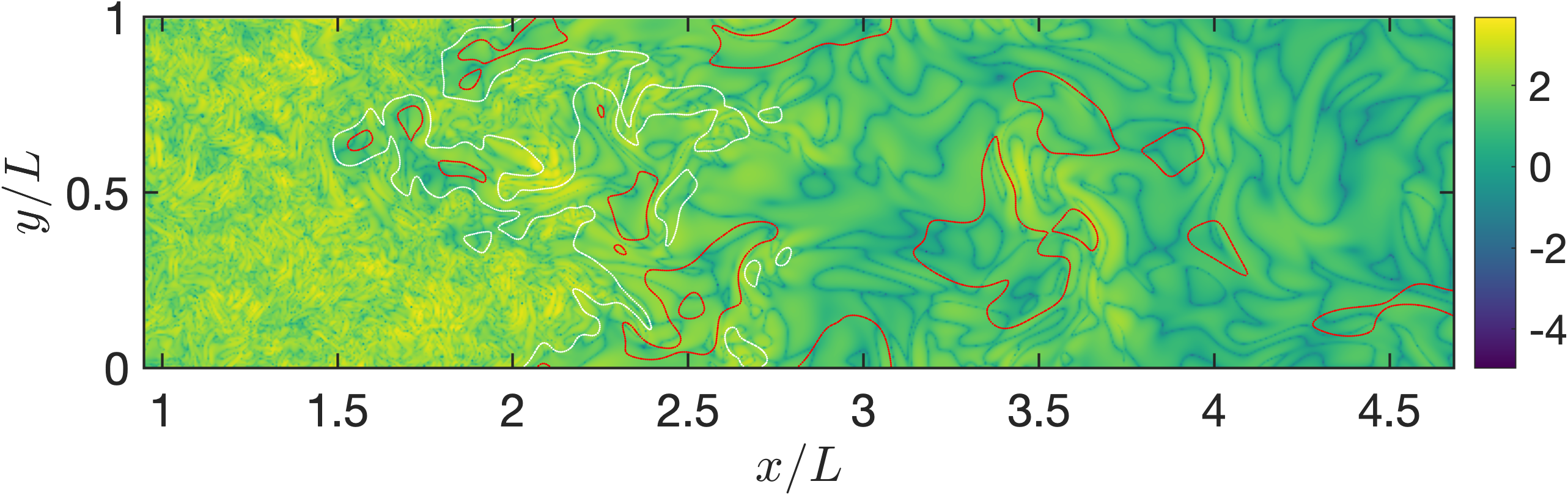
Figure 2: Instantaneous field of the difference in vorticity magnitude, $\log_{10}(|\omega_{\text{MA}}^{2}-\omega_{\text{MC}}^{2}|)$, between the mixture-averaged and multicomponent diffusion models for the lean premixed hydrogen-air flame examined here. Shown is the domain cross-section through the midplane. The red and white lines correspond to isosurfaces of $T_{0}=T_{\text{peak}}-$300\text{\,}\mathrm{K}\text{/}$$ and $T_{f}=T_{\text{peak}}+$300\text{\,}\mathrm{K}\text{/}$$, respectively, representing the inflow and outflow surfaces of the flame front.

As expected, the mixture-averaged and multicomponent contours in Fig. 1 exhibit little difference for a single time step. However, as shown in Fig. 2, if we examine the difference in the vorticity magnitude as an indicator of the relative impact of diffusion model on turbulent transport through the flame, the two cases notably disagree even after only a single time step. Although qualitative, Fig. 2 highlights the impact that diffusion model can have on the turbulent flow, thereby impacting turbulence-flame interactions at these high-Karlovitz conditions. On average, these differences can result in a significant and measurable difference in global flame statistics.

3.2 Enstrophy dynamics

To begin the analysis of enstrophy dynamics, we first consider time- and spatially averaged enstrophy ($\omega^{2}$) for the mixture-averaged and multicomponent simulations. We computed these statistics over 25 eddy turnover times ($\tau$), where $\tau=k/\epsilon\approx$ $500\text{\,}\mathrm{\SIUnitSymbolMicro s}\text{/}$, after first allowing the flames to develop in a turbulent flow field (ensuring that all transients from the initialization are lost). The spatial averages are calculated in $y$-$z$ spanwise planes along the $x$ direction.

Figure 3 shows that the small differences that appear in one time step (see Fig. 2) grow in magnitude over the course of the simulation. In particular, the mixture-averaged model underpredicts the peak enstrophy of the multicomponent diffusion model by up to $13\text{\,}\mathrm{\char 37\relax}\text{/}$ in the flame front. This difference suggests that the intensity of small-scale turbulence is generally lower in the mixture-averaged case, as compared to the corresponding multicomponent case. Moreover, the 13% quantitative difference in peak enstrophy shown in Fig. 3 closely matches the difference in mean turbulent flame speed in these flames shown previously by Fillo et al. [19].

However, for values of $x/\delta_{L}$ greater than roughly 3, Fig. 3 shows that the enstrophy in the mixture-averaged case is actually greater than in the multicomponent case. This corresponds to the super-adiabatic regions of the flame, discussed in Section 3.1, and indicates that the choice of mass diffusion model can have different relative effects on the local enstrophy magnitude at different locations in the high-Karlovitz, low-Lewis number premixed flames considered here.

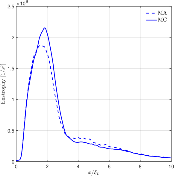
Figure 3: Time and spatially (spanwise) averaged enstrophy for multicomponent (MC) and mixture-averaged (MA) diffusion models.

To explain the differences in the vorticity magnitude/enstrophy when using mixture-averaged and multicomponent mass diffusion models, next we examine the transport equation for the enstrophy, which is obtained from the curl of the momentum equation in Eq. (2.1) as rCl 12Dω2Dt = ⏟ω⋅(ω⋅∇)u_Stretching - ⏟ω^2(∇⋅u)_Dilatation + ⏟ωρ2⋅(∇ρ×∇p)_Baroclinic torque + ⏟ω⋅∇×(1ρ∇⋅τ)_Viscous effects + ⏟ω⋅∇×fρ_Forcing  , where $D/Dt=\partial/\partial t+\bm{u}\cdot\nabla$ is the material derivative. The first term on the right-hand side of Eq. (3.2) represents vortex stretching, which is a nonlinear term accounting for the interaction between the strain rate and vorticity. The second term represents dilatation, which is primarily negative in reacting flows, suppressing vorticity magnitude. The third term represents baroclinic torque, which is only substantially nonzero when the gradients of density and pressure are both nonzero and misaligned. The fourth term represents viscous effects and includes contributions from both viscous diffusion and viscous dissipation. Finally, the last term represents the effect of the numerical body force present in Eq. (2.1).

Using data from both the mixture-averaged and multicomponent diffusion simulations, we compute time and spanwise averages of each term in Eq. (3.2) to examine the dynamical causes of the different enstrophy magnitudes shown in Figs. 2 and 3. Figure 4 shows the resulting normalized time- and spatially averaged enstrophy budgets, where we normalized following the approach by Bobbitt et al. [3].

Viscous effects are the primary sink term for both simulation cases and the primary source terms are vortex stretching, followed by forcing. For each of these physical effects, the multicomponent simulation yields larger peak magnitudes compared to the mixture-averaged simulation near the reaction zone of the flame (corresponding to the region close to $x/\delta_{L}\approx 2$). Interestingly, despite underpredicting the peak magnitudes of stretching, viscous, and forcing effects in the reaction zone, Fig. 4 shows that the mixture-averaged model overpredicts the viscous effects by as much as $13\text{\,}\mathrm{\char 37\relax}\text{/}$ in the super-adiabatic region of the flame (for values of $x/\delta_{L}$ greater than roughly 3). This difference between the two diffusion models mirrors the change in enstrophy within the super-adiabatic region shown in Fig. 3, and indicates that turbulence may thicken the flame in these super-adiabatic regions; this will be examined in more detail in the next section.

Finally, Fig. 4 shows that baroclinic torque is weakly positive and dilatation is weakly negative between $x/\delta_{L}\approx 2$–3 for both simulation cases, agreeing with prior studies of enstrophy dynamics in highly turbulent statistically planar premixed flames (see Steinberg et al. [41] for a review). Baroclinic torque can become the dominant term in the enstrophy dynamics when there is a persistent background pressure gradient, as in the tailored channel bluff body experiments by Geikie and Ahmed [42] and the swirl burner experiments by Kazbekov et al. [43, 44]. However, in unconfined statistically planar premixed flames such as those examined here, baroclinic torque becomes increasingly weak compared to stretching and viscous effects as the turbulence intensity increases [3]. The present results further show that, despite the differences between the multicomponent and mixture-averaged cases for the vortex stretching, viscous, and forcing terms, the baroclinic torque and dilatation terms are relatively unaffected by the choice of mass diffusion model.

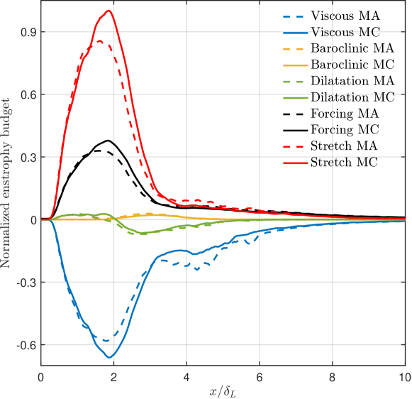
Figure 4: Time and spatially (spanwise) averaged enstrophy budgets for multicomponent (MC) and mixture-averaged (MA) diffusion models.

3.3 Flame width and reconstruction

To evaluate the impact of the observed differences in turbulence dynamics on the global flame structure, we reconstructed the average local internal structure of the turbulent flames. The reconstruction method used here was previously described by Hamlington et al. [1], and we refer the reader to that study for details. Briefly, the internal structure of the flame is connected to the magnitude of the temperature gradient, $\tilde{\chi}=(\nabla T\cdot\nabla T)^{1/2}/(T_{b}-T_{u})$, where $T_{b}$ and $T_{u}$ are the temperatures of the burnt and unburnt mixtures, respectively, in the corresponding laminar flame (see Table 1). Large $\tilde{\chi}$ indicates a thin flame and small $\tilde{\chi}$ indicates a broad flame [1, 45]. Correspondingly, we define $\delta_{t}=\tilde{\chi}^{-1}$ as the local turbulent flame width.

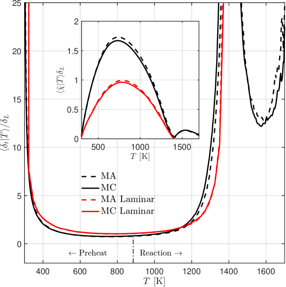
Figure 5: Conditional means of the local flame width $\langle\delta_{t}|T\rangle\equiv\langle\tilde{\chi}^{-1}|T\rangle$ normalized using the laminar flame thickness, $\delta_{L}$. The inset shows $\langle\tilde{\chi}|T\rangle$ normalized by $\delta_{L}$.

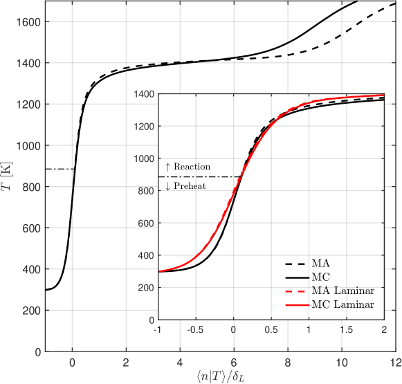
Figure 6: Average local flame structure reconstructed using $\langle\tilde{\chi}^{-1}|T\rangle$ from Fig. 5 and Eq. (6) for the turbulent and laminar flames with multicomponent and mixture-averaged mass diffusion. We chose $\langle n|T=T_{\mathrm{ref}}\rangle=0$ in Eq. (6) by requiring that $\langle n|T_{\mathrm{ref}}\rangle/\delta_{L}=0$ for all cases, where $T_{\mathrm{ref}}=T_{0}$ and $\langle n|T\rangle/\delta_{L}>0$ are locations closer to reactants and $\langle n|T\rangle/\delta_{L}<0$ are locations closer to products. The inset highlights the flame front to facilitate comparison with the average local laminar flame structure.

Figure 5 shows that for both the mixture-averaged and multicomponent models, the presence of turbulence thins the flame overall, which is expected in the thin-flame regime. Consistent with the contours shown in Figs. 1 and 2, we define the separation between the preheat and reaction zones based on the $T_{0}=T_{\mathrm{peak}}-$300\text{\,}\mathrm{K}\text{/}$$ isosurface. Both flames have similar widths in the preheat zone while the multicomponent flame is slightly thinner in the reaction zone. The value of $\langle\delta_{t}|T\rangle/\delta_{L}$ in Fig. 5 has a second minimum at $\sim$$1600\text{\,}\mathrm{K}\text{/}$, corresponding to the super-adiabatic region of the flame. At these high temperatures, the mixture-averaged flame is broader, consistent with the observed differences in viscous effects in Fig. 4. Values of $\langle\delta_{t}|T\rangle/\delta_{L}$ can be greater than one since $\delta_{L}\sim|\nabla T|^{-1}_{\mathrm{max}}$ corresponds to the minimum local width of the laminar flame, and both the turbulent and laminar widths exceed this at most locations.

Using the distributions of $\langle\delta_{t}|T\rangle$ in Fig. 5, we reconstruct the average local internal structure of the turbulent flames using the procedure outlined by Hamlington et al. [1]. The average flame-normal coordinate, $\langle n|T\rangle$, is calculated from $\langle\tilde{\chi}^{-1}|T\rangle/\delta_{L}$ as

$$\langle n|T\rangle=\langle n|T=T_{\mathrm{ref}}\rangle+\int_{0}^{T}\langle\tilde{\chi}^{-1}|\eta\rangle d\eta\;,$$ (6)

where $\langle n|T=T_{\mathrm{ref}}\rangle$ is the location corresponding to $T_{\mathrm{ref}}=T_{0}$, taken as the transition between the preheat and reaction zones for the present flames. Integrating Eq. (6) gives profiles of $T$ as a function of $\langle n|T\rangle$, which approximate the internal structure of the turbulent flame.

The resulting profiles in Fig. 6 show that the preheat zone thins for the turbulent flames and confirms that the multicomponent flame is slightly broader in the reaction zone. Moreover, Fig. 6 shows that the super-adiabatic regions of the mixture-averaged flame are as much as $18\text{\,}\mathrm{\char 37\relax}\text{/}$ broader than in the multicomponent flame. This large difference in flame structure indicates that mixture-averaged diffusion may not fully capture the complex interaction between diffusion and turbulent transport in high-temperature regions of the flame where steep gradients in the scalar field are present.

These differences may be explained by considering the underlying mathematical forms of the two diffusion models. As shown in Eq. (2), the direction of the mixture-averaged diffusion flux vector is strictly aligned counter to the species gradient vector. Thus, species can only diffuse down the species gradient from high concentration to low concentration. Alternatively, as shown in Eq. (5), the multicomponent diffusion model does not restrict the direction of the diffusion flux vector. In this case, diffusion can occur in multiple directions simultaneously, corresponding to the full scalar field.

Physically, this means that any small-scale changes in the mixture-averaged velocity field—on the order of viscous effects—must also be limited in their direction. By limiting the direction of diffusion, the magnitude of mass transport must increase to account for any diffusion not aligned with the species gradient in the multicomponent case. Aggregating diffusion flux into a single direction may change the direction of local velocity, redistributing mass and momentum.

4 Conclusions

In this study, we assessed the impact of mixture-averaged and multicomponent species diffusion models on turbulent enstrophy dynamics and average local flame structure for 3D, premixed, high-Karlovitz, lean hydrogen/air flames. We observed small differences when comparing the total vorticity magnitude for the two flames even after one time step, suggesting that the mixture-averaged diffusion assumption may not fully model the physical mass transport of the full multicomponent case. These differences grow over time, leading to a difference in enstrophy of up to $13\text{\,}\mathrm{\char 37\relax}\text{/}$ in the flame front.

Additional time- and spatially averaged analyses of enstrophy transport show significant differences in vortex stretching and viscous effects between the two models. Specifically, using the mixture-averaged model underpredicts the viscous effects and vortex stretching terms of the enstrophy budget by $13\text{\,}\mathrm{\char 37\relax}\text{/}$ and $17\text{\,}\mathrm{\char 37\relax}\text{/}$, respectively, in the flame front.

Variations in the vortex structure and viscous terms reappear in the super-adiabatic regions of the flame. These differences seem to contribute to significant broadening of the mixture-averaged flame relative to the multicomponent flame in these regions. Thus, although the mixture-averaged diffusion model may adequately reproduce full multicomponent mass diffusion in the preheat and reaction zones, it may fail to appropriately model mass transport in high-temperature, thermally unstable regions of the flame. The strict alignment of the mixture-averaged diffusion vector with the species counter-gradient may increase the local velocity and steepen velocity gradients, corresponding to an overprediction in the viscous dissipation.

These results suggest that although the mixture-averaged diffusion model may reasonably approximate full multicomponent diffusion, care should be taken in applying it, particularly in high-Karlovitz, low-Lewis number flames similar to those examined here.

Additional study is needed to determine whether stoichiometric or rich premixed flames show corresponding effects, and whether diffusion flames are similarly affected. Previously, Fillo et al. [19] found differences in the characteristics of nearly stoichiometric hydrocarbon flames when using mixture-averaged and multicomponent diffusion models, and corresponding differences are likely present in the enstrophy dynamics. Burali et al. [30] showed that using a set of constant non-unity Lewis numbers produces only small errors in ethylene/air diffusion flames, as compared with mixture-averaged simulations, suggesting that there may be only slight differences between mixture-averaged and multicomponent models in diffusion flames. Further studies should be performed in the future to determine the relative impacts of mixture-averaged and multicomponent diffusion models on enstrophy dynamics for a broader range of configurations and combustion conditions.

Funding

This material is based upon work supported by the National Science Foundation under Grant Nos. 1314109-DGE and 1761683. KEN also acknowledges support from the Welty Faculty Fellowship at Oregon State University. PEH was supported, in part, by AFOSR Award No. FA9550–17-1–0144 and NSF Award No. 1847111. This research used resources of the National Energy Research Scientific Computing Center, a DOE Office of Science User Facility supported by the Office of Science of the U.S. Department of Energy under Contract No. DE-AC02-05CH11231.

Appendix A Availability of material

The figures in this article, as well as the data and plotting scripts necessary to reproduce them, are available openly under the CC-BY license [46]. Furthermore, the full simulation inputs for and output data produced by NGA are available [47].

References

- [1] P.E. Hamlington, A.Y. Poludnenko, and E.S. Oran, Interactions between turbulence and flames in premixed reacting flows, Phys. Fluids 23 (2011), p. 125111, https://doi.org/10.1063/1.3671736.
- [2] N. Chakraborty, I. Konstantinou, and A. Lipatnikov, Effects of Lewis number on vorticity and enstrophy transport in turbulent premixed flames, Phys. Fluids 28 (2016), p. 015109, https://doi.org/10.1063/1.4939795.
- [3] B. Bobbitt, S. Lapointe, and G. Blanquart, Vorticity transformation in high Karlovitz number premixed flames, Phys. Fluids 28 (2016), p. 015101, https://doi.org/10.1063/1.4937947.
- [4] R.B. Bird, W.E. Stewart, and E.N. Lightfoot, Transport Phenomena, John Wiley & Sons, Inc., New York, 1960.
- [5] A.N. Lipatnikov and J. Chomiak, Molecular transport effects on turbulent flame propagation and structure, Progress in Energy and Combustion Science 31 (2005), pp. 1–73, https://doi.org/10.1016/j.pecs.2004.07.001.
- [6] M. Day, J. Bell, P.T. Bremer, V. Pascucci, V. Beckner, and M. Lijewski, Turbulence effects on cellular burning structures in lean premixed hydrogen flames, Combustion and Flame 156 (2009), pp. 1035–1045, https://doi.org/10.1016/j.combustflame.2008.10.029.
- [7] A.J. Aspden, M.S. Day, and J.B. Bell, Turbulence-flame interactions in lean premixed hydrogen: Transition to the distributed burning regime, J. Fluid Mech. 680 (2011), pp. 287–320, https://doi.org/10.1017/jfm.2011.164.
- [8] A. Aspden, A numerical study of diffusive effects in turbulent lean premixed hydrogen flames, Proc. Combust. Inst. 36 (2017), pp. 1997–2004, https://doi.org/10.1016/j.proci.2016.07.053.
- [9] J. Schlup and G. Blanquart, Validation of a mixture-averaged thermal diffusion model for premixed lean hydrogen flames, Combustion Theory and Modelling 22 (2018), pp. 264–290, https://doi.org/10.1080/13647830.2017.1398350.
- [10] T. Coffee and J. Heimerl, Transport algorithms for premixed, laminar steady-state flames, Combust. Flame 43 (1981), pp. 273–289, https://doi.org/10.1016/0010-2180(81)90027-4.
- [11] A. Ern and V. Giovangigli, Thermal diffusion effects in hydrogen-air and methane-air flames, Combust. Theor. Model. 2 (1998), pp. 349–372, https://doi.org/10.1088/1364-7830/2/4/001.
- [12] A. Ern and V. Giovangigli, Impact of detailed multicomponent transport on planar and counterflow hydrogen/air and methane/air flames, Combust. Sci. Technol. 149 (1999), pp. 157–181, https://doi.org/10.1080/00102209908952104.
- [13] H. Bongers and L. De Goey, The effect of simplified transport modeling on the burning velocity of laminar premixed flames, Combust. Sci. Technol. 175 (2003), pp. 1915–1928, https://doi.org/10.1080/713713111.
- [14] F. Yang, C. Law, C. Sung, and H. Zhang, A mechanistic study of Soret diffusion in hydrogen–air flames, Combust. Flame 157 (2010), pp. 192–200, https://doi.org/10.1016/j.combustflame.2009.09.018.
- [15] Y. Xin, C.J. Sung, and C.K. Law, A mechanistic evaluation of Soret diffusion in heptane/air flames, Combust. Flame 159 (2012), pp. 2345–2351, https://doi.org/10.1016/j.combustflame.2012.03.005.
- [16] V. Giovangigli, Multicomponent transport in laminar flames, Proc. Combust. Inst. 35 (2015), pp. 625–637, https://doi.org/10.1016/j.proci.2014.08.011.
- [17] S. Dworkin, M. Smooke, and V. Giovangigli, The impact of detailed multicomponent transport and thermal diffusion effects on soot formation in ethylene/air flames, Proc. Combust. Inst. 32 (2009), pp. 1165–1172, https://doi.org/10.1016/j.proci.2008.05.061.
- [18] Y. Xin, W. Liang, W. Liu, T. Lu, and C.K. Law, A reduced multicomponent diffusion model, Combust. Flame 162 (2015), pp. 68–74, https://doi.org/10.1016/j.combustflame.2014.07.019.
- [19] A.J. Fillo, J. Schlup, G. Blanquart, and K.E. Niemeyer, Assessing the impact of multicomponent diffusion in direct numerical simulations of premixed, high-karlovitz, turbulent flames, Combustion and Flame 223 (2021), pp. 216–229, https://doi.org/10.1016/j.combustflame.2020.09.013.
- [20] O. Desjardins, G. Blanquart, G. Balarac, and H. Pitsch, High order conservative finite difference scheme for variable density low Mach number turbulent flows, J. Comput. Phys. 227 (2008), pp. 7125–7159, https://doi.org/10.1016/j.jcp.2008.03.027.
- [21] B. Savard, Y. Xuan, B. Bobbitt, and G. Blanquart, A computationally-efficient, semi-implicit, iterative method for the time-integration of reacting flows with stiff chemistry, J. Comput. Phys. 295 (2015), pp. 740–769, https://doi.org/10.1016/j.jcp.2015.04.018.
- [22] A.J. Fillo, J. Schlup, G. Beardsell, G. Blanquart, and K.E. Niemeyer, A fast, low-memory, and stable algorithm for implementing multicomponent transport in direct numerical simulations, Journal of Computational Physics 406 (2020), p. 109185, https://doi.org/10.1016/j.jcp.2019.109185.
- [23] C.F. Curtiss and J.O. Hirschfelder, Transport properties of multicomponent gas mixtures, J. Chem. Phys. 17 (1949), pp. 550–555, https://doi.org/10.1063/1.1747319.
- [24] J.O. Hirschfelder, C.F. Curtiss, and R.B. Bird, Molecular Theory of Gases and Liquids, Wiley, New York, 1954.
- [25] J.F. Grcar, J.B. Bell, and M.S. Day, The Soret effect in naturally propagating, premixed, lean, hydrogen–air flames, Proc. Combust. Inst. 32 (2009), pp. 1173–1180, https://doi.org/10.1016/j.proci.2008.06.075.
- [26] R.J. Kee, M.E. Coltrin, P. Glarborg, and H. Zhu, Chemically Reacting Flow, 2nd ed., John Wiley & Sons, Inc, 2018.
- [27] V. Giovangigli, Convergent iterative methods for multicomponent diffusion, IMPACT of Computing in Science and Engineering 3 (1991), pp. 244–276, https://doi.org/10.1016/0899-8248(91)90010-r.
- [28] R. Kee, F. Rupley, and J. Miller, Chemkin-II: A Fortran chemical kinetics package for the analysis of gas-phase chemical kinetics, Sandia National Laboratories Report SAND89-8009 (1989). https://doi.org/10.2172/5681118.
- [29] G. Dixon-Lewis, Flame structure and flame reaction kinetics. II. transport phenomena in multicomponent systems, Proc. Royal Soc. A 307 (1968), https://doi.org/10.1098/rspa.1968.0178.
- [30] N. Burali, S. Lapointe, B. Bobbitt, G. Blanquart, and Y. Xuan, Assessment of the constant non-unity Lewis number assumption in chemically-reacting flows, Combust. Theor. Model. 20 (2016), pp. 632–657, https://doi.org/10.1080/13647830.2016.1164344.
- [31] S. Lapointe and G. Blanquart, Fuel and chemistry effects in high Karlovitz premixed turbulent flames, Combust. Flame 167 (2016), pp. 294–307, https://doi.org/10.1016/j.combustflame.2016.01.035.
- [32] Z. Hong, D.F. Davidson, and R.K. Hanson, An improved H2/O2 mechanism based on recent shock tube/laser absorption measurements, Combust. Flame 158 (2011), pp. 633–644, https://doi.org/10.1016/j.combustflame.2010.10.002.
- [33] K.Y. Lam, D.F. Davidson, and R.K. Hanson, A shock tube study of H2 + OH H2O + H using OH laser absorption, Int. J. Chem. Kinet. 45 (2013), pp. 363–373, https://doi.org/10.1002/kin.20771.
- [34] Z. Hong, K.Y. Lam, R. Sur, S. Wang, D.F. Davidson, and R.K. Hanson, On the rate constants of OH + HO2 and HO2 + HO2: A comprehensive study of H2O2 thermal decomposition using multi-species laser absorption, Proc. Combust. Inst. 34 (2013), pp. 565–571, https://doi.org/10.1016/j.proci.2012.06.108.
- [35] B. Savard and G. Blanquart, Broken reaction zone and differential diffusion effects in high Karlovitz n-C7H16 premixed turbulent flames, Combust. Flame 162 (2015), pp. 2020–2033, https://doi.org/10.1016/j.combustflame.2014.12.020.
- [36] C. Rosales and C. Meneveau, Linear forcing in numerical simulations of isotropic turbulence: Physical space implementations and convergence properties, Phys. Fluids 17 (2005), p. 095106, https://doi.org/10.1063/1.2047568.
- [37] P.L. Carroll and G. Blanquart, A proposed modification to Lundgren’s physical space velocity forcing method for isotropic turbulence, Phys. Fluids 25 (2013), p. 105114, https://doi.org/10.1063/1.4826315.
- [38] M. Klein, N. Chakraborty, and S. Ketterl, A comparison of strategies for direct numerical simulation of turbulence chemistry interaction in generic planar turbulent premixed flames, Flow, Turbulence and Combustion 99 (2017), pp. 955–971, https://doi.org/10.1007/s10494-017-9843-9.
- [39] F.A. Williams, Combustion Theory, Benjamin/Cummings, 1985.
- [40] A. Aspden, M. Day, and J. Bell, Turbulence-chemistry interaction in lean premixed hydrogen combustion, Proc. Combust. Inst. 35 (2015), pp. 1321–1329, https://doi.org/10.1016/j.proci.2014.08.012.
- [41] A.M. Steinberg, P.E. Hamlington, and X. Zhao, Structure and dynamics of highly turbulent premixed combustion, Progress in Energy and Combustion Science 85 (2021), p. 100900, https://doi.org/10.1016/j.pecs.2020.100900.
- [42] M.K. Geikie and K.A. Ahmed, Pressure-gradient tailoring effects on the turbulent flame-vortex dynamics of bluff-body premixed flames, Combustion and Flame 197 (2018), pp. 227–242, https://doi.org/10.1016/j.combustflame.2018.08.001.
- [43] A. Kazbekov, K. Kumashiro, and A.M. Steinberg, Enstrophy transport in swirl combustion, Journal of Fluid Mechanics 876 (2019), pp. 715–732, https://doi.org/10.1017/jfm.2019.551.
- [44] A. Kazbekov and A.M. Steinberg, Flame- and flow-conditioned vorticity transport in premixed swirl combustion, Proceedings of the Combustion Institute 38 (2021), pp. 2949–2956, https://doi.org/10.1016/j.proci.2020.06.211.
- [45] S.H. Kim and H. Pitsch, Scalar gradient and small-scale structure in turbulent premixed combustion, Phys. Fluids 19 (2007), p. 115104, https://doi.org/10.1063/1.2784943.
- [46] A.J. Fillo, P.E. Hamlington, and K.E. Niemeyer, Figures, plotting scripts, and data for “Assessing diffusion model impacts on turbulent transport and flame structure in lean premixed flames” [dataset], Zenodo (2022). https://doi.org/10.5281/zenodo.6191166.
- [47] A.J. Fillo, P.E. Hamlington, and K.E. Niemeyer, Assessing the impact of diffusion model on the turbulent transport and flame structure of premixed lean hydrogen flames: hydrogen data (version 1) [dataset], Oregon State University (2020). https://doi.org/10.7267/37720k356.