PerceMon: Online Monitoring for Perception Systems

Abstract

Perception algorithms in autonomous vehicles are vital for the vehicle to understand the semantics of its surroundings, including detection and tracking of objects in the environment. The outputs of these algorithms are in turn used for decision-making in safety-critical scenarios like collision avoidance, and automated emergency braking. Thus, it is crucial to monitor such perception systems at runtime. However, due to the high-level, complex representations of the outputs of perception systems, it is a challenge to test and verify these systems, especially at runtime. In this paper, we present a runtime monitoring tool, PerceMon that can monitor arbitrary specifications in Timed Quality Temporal Logic (TQTL) and its extensions with spatial operators. We integrate the tool with the CARLA autonomous vehicle simulation environment and the ROS middleware platform while monitoring properties on state-of-the-art object detection and tracking algorithms.

1 Introduction

In recent years, the popularity of autonomous vehicles has increased greatly. With this popularity, there has also been increased attention drawn to the various fatalities caused by the autonomous components on-board the vehicles, especially the perception systems [24, 16]. Perception modules on these vehicles use vision data from cameras to reason about the surrounding environment, including detecting objects and interpreting traffic signs, and in-turn used by controllers to perform safety-critical control decisions, including avoiding pedestrians. Due to the nature of these systems, it has become important that these systems be tested during design and monitored during deployment.

Signal temporal logic (STL) [17] and Metric Temporal Logic (MTL) [11] have been used extensively in verification, testing, and monitoring of safety-critical systems. In these scenarios, typically there is a model of the system that is generating trajectories under various actions. These traces are the used to test if the system satisfies some specification. This is referred to as offline monitoring, and is the main setting for testing and falsification of safety-critical systems. On the other hand, STL and MTL have been used for online monitoring where some safety property is checked for compliance at runtime [19, 6]. These are used to express rich specifications on low-level properties of signals outputted from systems.

The output of a perception algorithm consists of a sequence of frames, where each frame contains a variable number of objects over a fixed set of categories, in addition to object attributes that can range over larger data domains (e.g. bounding box coordinates, distances, confidence levels, etc.). STL and MTL can handle mixed-mode signals and there have been attempts to extend them to incorporate spatial data [3, 18, 13]. However, these logics lack the ability to compare objects in different frames, or model complex spatial relations between objects.

Timed Quality Temporal Logic (TQTL) [5], and Spatio-temporal Quality Logic (STQL) [14] are extensions to MTL that incorporate the semantics for reasoning about data from perception systems specifically. In STQL, which is in itself an extension of TQTL, the syntax defines operators to reason about discrete IDs and classes of objects, along with set operations on the spatial artifacts, like bounding boxes, outputted by perception systems.

In this project, we contribute the following:

1. We show how TQTL [5] and STQL [14] can be used to express correctness properties for perception algorithms.

2. An online monitoring tool, PerceMon, that efficiently monitors STQL specifications. We integrate this tool with the CARLA simulation environment [8] and the Robot Operating System (ROS) [20].

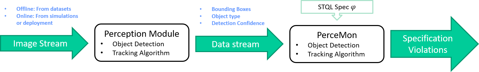
Figure 1: The PerceMon online monitoring pipeline.

Related work

S-TaLiRo [2, 10], VerifAI [9] and Breach [7] are some examples of tools used for offline monitoring of MTL and STL specifications. The presented tool, PerceMon, models its architecture similar to the RTAMT [19] online monitoring tool for STL specifications: the core tool is written in C++ with an interface for use in different, application-specific platforms.

2 Spatio-temporal Quality Logic

Spatio-temporal quality logic (STQL) [14] is an extension of Timed Quality Temporal Logic (TQTL) [5] that incorporates reasoning about high-level topological structures present in perception data, like bounding boxes, and set operations over these structures.

STL has been used extensively in testing and monitoring of control systems mainly due to the ability to express rich specifications on low-level, real-valued signals generated from these systems. To make the logic more high-level, spatial extensions have been proposed that are able to reason about spatial relations between signals [3, 18, 12, 13]. A key feature of data streams generated by perception algorithms is that they contain frames of spatial objects consisting of both, real-values and discrete-valued quantities: the discrete-valued signals are the IDs of the objects and their associated categories; while real-valued signals include bounding boxes describing the objects and confidence associated with their identities. While STL and MTL can be used to reason about properties of a fixed number of such objects in each frame by creating signal variables to encode each of these properties, it is not possible to design monitors that handle arbitrarily many objects per frame.

TQTL [5] is a logic that is specifically catered for spatial data from perception algorithms. Using Timed Propositional Temporal Logic [4] as a basis, TQTL allows one to pin or freeze the signal at a certain time point and use clock variables associated with the freeze operator to define time constraints. Moreover, TQTL introduces a quantifier over objects in a frame and the ability to refer to properties intrinsic to the object: tracking IDs, classes or categories, and detection confidence. STQL [14] further extends the logic to reason about the bounding boxes associated with these objects, along with predicate functions for these spatial sets, by incorporating topological semantics from the $S4_{u}$ spatio-temporal logic [12].

Definition 1 (STQL Syntax [14])

Let $V_{t}$ be a set of time variables, $V_{f}$ be a set of frame variables, and $V_{o}$ be a set of object ID variables. Then the syntax for STQL is recursively defined by the following grammar:

$$\varphi::=\quad \exists\{{id}_{1},{id}_{2},\ldots\}@\varphi\mid\{x,f\}.\varphi$$

$$\mid\top\mid\neg\varphi\mid\varphi\lor\varphi\mid\operatorname{\bigcirc}\varphi\mid\operatorname{{\hbox to0.0pt{\hbox to10.00002pt{\hss--\hss}\hss}\hbox{$\bigcirc$}}}\varphi\mid\varphi\mathbin{\mathbf{U}}\varphi\mid\varphi\mathbin{\mathbf{S}}\varphi$$

$$\mid\textsf{C\_TIME}-x\sim t\mid\textsf{C\_FRAME}-f\sim n$$

$$\mid\operatorname{\mathsf{C}}({id}_{i})=c\mid\operatorname{\mathsf{C}}({id}_{i})=\operatorname{\mathsf{C}}({id}_{i})\mid\operatorname{\mathsf{P}}({id}_{i})\geq r\mid\operatorname{\mathsf{P}}({id}_{i})\geq r\times\operatorname{\mathsf{P}}({id}_{j})$$

$$\mid\{{id}_{i}={id}_{j}\}\mid\{{id}_{i}\not={id}_{j}\}\mid\operatorname{{\hbox to0.0pt{\hbox to9.72224pt{\hss$\scalebox{0.7}{$\exists$}$\hss}\hss}\hbox{$\raisebox{-1.5pt}{\scalebox{1.25}{$\square$}}$}}}\Omega\mid\Pi$$

$$\Omega::=\quad \varnothing\mid\mathbb{U}\mid\operatorname{\mathfrak{BB}}({id}_{1})\mid\overline{\Omega}\mid\Omega\sqcup\Omega$$

$$\Pi::=\quad \operatorname{\mathsf{Area}}(\Omega)\geq r|\operatorname{\mathsf{Area}}(\Omega)\geq r\times\operatorname{\mathsf{Area}}(\Omega)$$

$$\mid\operatorname{\mathsf{ED}}({id}_{i},\mathrm{CRT},{id}_{j},\mathrm{CRT})\geq r\mid\Theta\geq r\mid\Theta\geq r\times\Theta$$

$$\Theta::=\quad \operatorname{\mathsf{Lat}}({id}_{i},\mathrm{CRT})\mid\operatorname{\mathsf{Lon}}({id}_{i},\mathrm{CRT})$$

$$\mathrm{CRT}::=\quad \mathsf{LM}\mid\mathsf{RM}\mid\mathsf{TM}\mid\mathsf{BM}\mid\mathsf{CT}$$

Here, ${id}_{i}\in V_{o}$ (for all indices $i$), $x\in V_{t}$, and $f\in V_{f}$. In the above grammar $r$ is a real-valued constant that allows for the comparison of ratios of object properties.

In the above grammar, $\neg\varphi$ and $\varphi\lor\varphi$ are, respectively, the negation and disjunction operators from propositional logic while $\operatorname{\bigcirc}\varphi$, $\operatorname{{\hbox to0.0pt{\hbox to10.00002pt{\hss--\hss}\hss}\hbox{$\bigcirc$}}}\varphi$, $\varphi\mathbin{\mathbf{U}}\varphi$, and $\varphi\mathbin{\mathbf{S}}\varphi$ are the temporal operators next, previous, until, and since respectively. The above grammar can be further used to derive the other propositional operators, like conjunction ($\varphi\land\varphi$), along with temporal operators like always ($\operatorname{\raisebox{-1.5pt}{\scalebox{1.25}{$\square$}}}\varphi$) and eventually ($\operatorname{\raisebox{-1.5pt}{\scalebox{1.25}{$\lozenge$}}}\varphi$), and their past-time equivalents holds ($\operatorname{{\hbox to0.0pt{\hbox to9.72224pt{\hss--\hss}\hss}\hbox{$\raisebox{-1.5pt}{\scalebox{1.25}{$\square$}}$}}}\varphi$) and once ($\operatorname{{\hbox to0.0pt{\hbox to8.33336pt{\hss-\hss}\hss}\hbox{$\raisebox{-1.5pt}{\scalebox{1.25}{$\lozenge$}}$}}}\varphi$). In addition to that, STQL extends these by introducing freeze quantifiers over clock variables and object variables. $\{x,f\}.\varphi$ freezes the time and frame that the formula $\varphi$ is evaluated, and assigns them to the clock variables $x$ and $f$, where $x$ refers to pinned time variables and $f$ refers to pinned frame variables. The constants, $\textsf{C\_TIME},\textsf{C\_FRAME}$ refer to the value of the time and frame number where the current formula is being evaluated. This allows for the expression $x-\textsf{C\_TIME}$ and $f-\textsf{C\_FRAME}$ to measure the duration and the number of frames elapsed, respectively, since the clock variables $x$ and $f$ were pinned. The expression $\exists\{{id}_{1}\}@\varphi$ searches over each object in a frame in the incoming data stream — assigning each object to the object variable ${id}_{1}$ — if there exists an object that satisfies $\varphi$. The functions $\operatorname{\mathsf{C}}(id)$ and $\operatorname{\mathsf{P}}(id)$ refer to the class and confidence the detected object associated with the ID variable. In addition to these TQTL operations, bounding boxes around objects can be extracted using the expression $\operatorname{\mathfrak{BB}}(id)$ and set topological operations can be defined over them. The spatial exists operator $\operatorname{{\hbox to0.0pt{\hbox to9.72224pt{\hss$\scalebox{0.7}{$\exists$}$\hss}\hss}\hbox{$\raisebox{-1.5pt}{\scalebox{1.25}{$\square$}}$}}}\Omega$ checks if the spatial expression $\Omega$ results in a non-empty space or not. Quantitative operations like $\operatorname{\mathsf{Area}}(\cdot)$ measure the area of spatial sets; $\operatorname{\mathsf{ED}}$ computes the Euclidean distances between references points ($\mathrm{CRT}$) of bounding boxes; and $\operatorname{\mathsf{Lat}}$ and $\operatorname{\mathsf{Lon}}$ measure the latitudinal and longitudinal offset of bounding boxes respectively. Here, $\mathrm{CRT}$ refers to the reference points — left, right, top, and bottom margins, and the centroid — for bounding boxes. Due to lack of space, we defer defining the formal semantics of STQL to Appendix 0.A and also refer the readers to [14] for more extensive details.

3 PerceMon: An Online Monitoring Tool

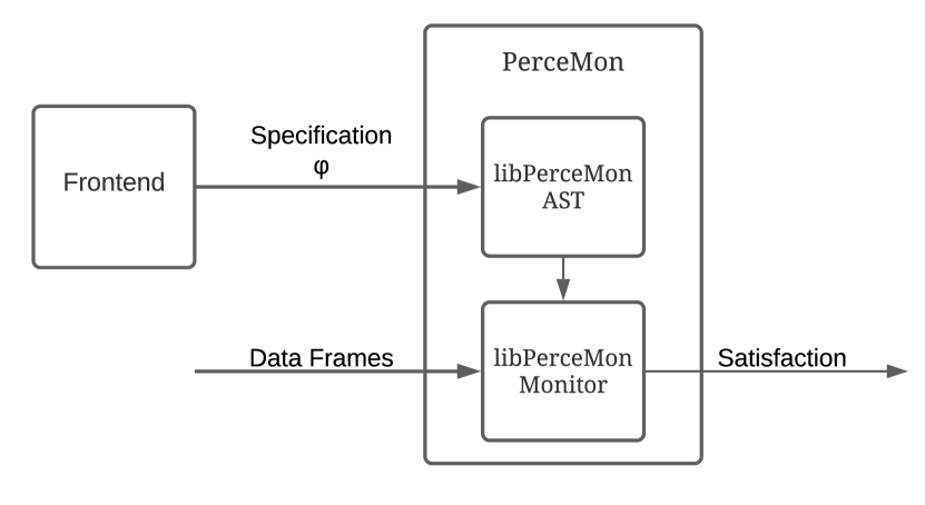
(a) General architecture for PerceMon. The frontend component is a generic wrapper around libPerceMon, the C++ library that provides the online monitoring functionality, for example, a wrapper for ROS, a parser from some specification language, or a Python library.

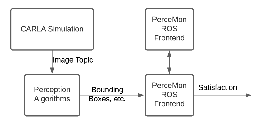
(b) Architecture of the integration of PerceMon with the CARLA autonomous vehicle simulator and ROS middleware platform.

PerceMon is an online monitoring tool for STQL specifications. It computes the quality of a formula $\varphi$ at the current evaluation frame, if $\varphi$ can be evaluated with some finite number of frames in the past (history) and delayed frames from the future (horizon).

The core of the tool consists of a C++ library, libPerceMon, which provides an interface to define an STQL abstract syntax tree efficiently, along with a general online monitor interface. The PerceMon tool works by initializing a monitor with a given STQL specification and can receive data in a frame-by-frame manner. It stores the frames in a first-in-first-out (FIFO) buffer with maximum size defined by the horizon and history requirement of the specification. This enables fast and efficient computation of the quality of the formula for the bounded horizon. An overview of the architecture can be seen in 2(a).

The library, libPerceMon, designed with the intention to be used with wrappers that convert application-specific data to data structures supported by the library (signified by the “Frontend” block in the architecture presented in 2(a)). In the subsequent section, we show an example of how such an integration can be performed by interfacing libPerceMon with the CARLA autonomous vehicle simulator [8] via the ROS middleware platform [20].

3.1 Integration with CARLA and ROS

In this section, we present an integration of the PerceMon tool with the CARLA autonomous vehicle simulator [8] using the ROS middleware platform [20]. This follows the example of [9] and [26] which interface with CARLA, and [19], where the tool interfaces with the ROS middleware platform for use in online monitoring applications.

The CARLA simulator is an autonomous vehicle simulation environment that uses high-quality graphics engines to render photo-realistic scenes for testing such vehicles. Pairing this with ROS allows us to abstract the data generated by the simulator, the PerceMon monitor, and various perception modules as streams of data or topics in a publisher-subscriber network model. Here, a publisher broadcasts data in a known binary format at an endpoint (called a topic) without knowing who listens to the data. Meanwhile, a subscriber registers to a specific topic and listens to the data published on that endpoint.

In our framework, we use the ROS wrapper for CARLA to publish all the information from the simulator, including data from the cameras on the autonomous vehicle. The image data is used by perception modules — like the YOLO object detector [22] and the DeepSORT object tracker [25] — to publish processed data. The information published by these perception modules can in-turn be used by other perception modules (like using detected objects to track them), controllers (that may try to avoid collisions), and by PerceMon online monitors. The architectural overview can be seen in 2(b).

The use of ROS allows us to reason about data streams independent of the programming languages that the perception modules are implemented in. For example, the main implementation of the YOLO object detector is written in C/C++ using a custom deep neural network framework called Darknet [21], while the DeepSORT object tracker is implemented in Python. The custom detection formats from each of these algorithms can be converted into standard messages that are published on predefined topics, which are then subscribed to from PerceMon. Moreover, this also paves the way to migrate and apply PerceMon to any other applications that use ROS for perception-based control, for example, in the software stack deployed on real-world autonomous vehicles [15].

4 Experiments

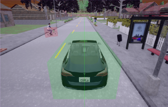
(a) In this scenario, the configuration is such that the sun has set. In a poorly lit road, a cyclist tries to cross the road.

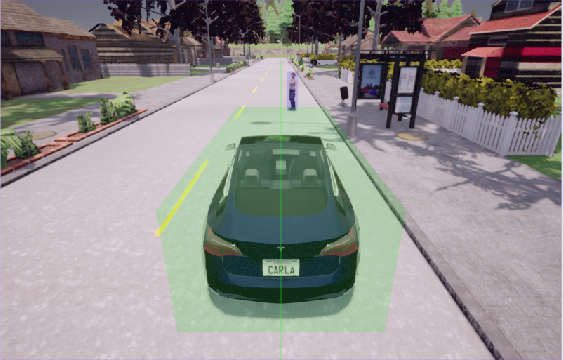
(b) Here, a partially occluded pedestrian decides to suddenly cross the road as the vehicle cruises down the street.

Figure 3: The presented scenarios simulated in CARLA aim to demonstrate some common failures associated with deep neural network-based perception modules. These include situations where partially occluded objects are not detected or tracked properly, and situations where different lighting conditions cause mislabeling of detected objects. In both the above scenarios, we also add some passive vehicles to increase the number of objects detected in any frame. This allows us to compute the time it takes to compute the satisfaction values from the monitor as the number of objects that need to be checked increases.

In this section, we present a set of experiments using the integration of PerceMon with the CARLA autonomous car simulator [8] presented in Section 3.1. We build on the ROS-based architecture described in the previous section, and monitor the following perception algorithms:

• Object Detection: The YOLO object detector [22, 23] is a deep convolutional neural networks (CNN) based model that takes as input raw images from the camera and outputs a list of bounding boxes for each object in the image.

• Object Tracking: The SORT object tracker [25] takes the set of detections from the object detector and associates an ID with each of them. It then tries to track each annotated object across frames using Kalman filters and cosine association metrics.

We use the OpenSCENARIO specification format [1] to define scenarios in the CARLA simulation that mimic some real-world, accident-prone scenarios, where there have been several instances where deep neural network based perception algorithms fail at detecting or tracking pedestrians, cyclists, and other vehicles. To detect some common failure cases, we initialize the PerceMon monitors with the following specifications:

Consistent Detections $\varphi_{1}$

: For all objects in the current frame that have high confidence, if the object is far away from the margins, then the object must have existed in the previous frame too with sufficiently high confidence.

$$\begin{split}\varphi_{1}&:=\forall\{id_{1}\}@\{f\}.\left(\left(\varphi_{\text{high prob}}\land\varphi_{\text{margins}}\right)\Rightarrow\operatorname{{\hbox to0.0pt{\hbox to10.00002pt{\hss--\hss}\hss}\hbox{$\bigcirc$}}}\varphi_{\text{exists}}\right)\\ \varphi_{\text{high prob}}&:=\operatorname{\mathsf{P}}(id_{1})>0.8\\ \varphi_{\text{margins}}&:=\operatorname{\mathsf{Lon}}(id_{1},\mathsf{TM})>c_{1}\land\operatorname{\mathsf{Lon}}(id_{1},\mathsf{BM})<c_{2}\\ &\quad\land\operatorname{\mathsf{Lat}}(id_{1},\mathsf{LM})>c_{3}\land\operatorname{\mathsf{Lat}}(id_{1},\mathsf{RM})<c_{4}\\ \varphi_{\text{exists}}&:=\exists\{id_{2}\}.\left(\{id_{1}=id_{2}\}\land\operatorname{\mathsf{P}}(id_{2})>0.7\right)\end{split}$$ (1)

Object detection algorithms are known to frequently miss detecting objects in consecutive frames or detect them with low confidence after detecting them with high confidence in previous frames. This can cause issues with algorithms that rely on consistent detections, e.g., for obstacle tracking and avoidance. The above formula checks this for objects that we consider “relevant” (using $\varphi_{\text{margins}}$), i.e., the object is not too far away from the edges of the image. This allows us to filter false alarms from objects that naturally leave the field of view of the camera.

Smooth Object Trajectories $\varphi_{2}$

: For every object in the current frame, its bounding box and the corresponding bounding box in the previous frame must overlap more than 30%.

$$\begin{split}\varphi_{2}&:=\forall\{id_{1}\}@\{f_{1}\}.\left(\operatorname{{\hbox to0.0pt{\hbox to10.00002pt{\hss--\hss}\hss}\hbox{$\bigcirc$}}}\left(\exists\{id_{2}\}@\{f_{2}\}.\left(\{id_{1}=id_{2}\}\Rightarrow\varphi_{\text{overlap}}\right)\right)\right)\\ \varphi_{\text{overlap}}&:=\frac{\operatorname{\mathsf{Area}}(\operatorname{\mathfrak{BB}}(id_{1})\sqcap\operatorname{\mathfrak{BB}}(id_{2}))}{\operatorname{\mathsf{Area}}(\operatorname{\mathfrak{BB}}(id_{1}))}\geq 0.3\end{split}$$ (2)

In consecutive frames, if detected bounding boxes are sufficiently far apart, it is possible for tracking algorithms that rely on the detections to produce incorrect object associations, leading to poor information for decision-making.

We monitor the above properties for scenarios described in Figure 3, and check for the time it takes to compute the satisfaction values of the above properties. As each scenario consists of some passive or non-adversarial vehicles, the number of objects detected by the object detector increases. Thus, since the runtime for the STQL monitor is exponential in the number of object IDs referenced in the existential quantifiers, this allows us to empirically measure the amount of time it takes to compute the satisfaction value in the monitor. The number of simulated non-adversarial objects are ranged from 1 to 10, and the time taken to compute the satisfaction value for each new frame is recorded. We present the results in Table 1, and refer the readers to [14] for theoretical results on monitoring complexity for STQL specifications.

Table 1: Compute time for different properties, with increasing number of objects.

Average Number of Objects	Average Compute Time (s)
	$\varphi_{1}$	$\varphi_{2}$
2	$7.0\times 10^{-6}$	$7.3\times 10^{-6}$
5	$1.4\times 10^{-5}$	$2.3\times 10^{-5}$
10	$5.4\times 10^{-4}$	$6.3\times 10^{-4}$

5 Conclusion

In this paper, we presented PerceMon, an online monitoring library and tool for generating monitors for specifications given in Spatio-temporal Quality Logic (STQL). We also present a set of experiments that make use of PerceMon’s integration with the CARLA autonomous car simulator and the ROS middleware platform.

In future iterations of the tool, we hope to incorporate a more expressive version of the specification grammar that can reason about arbitrary spatial constructs, including oriented polygons and segmentation regions, and incorporate ways to formally reason about system-level properties (like system warnings and control inputs).

Appendix 0.A Semantics for STQL

Consider a data stream $\xi$ consisting of frames containing objects and annotated with a time stamp. Let $i\in\mathbb{N}$ be the current frame of evaluation, and let $\xi_{i}$ denote the $i^{th}$ frame. We let $\epsilon:V_{t}\cup V_{f}\to\mathbb{N}\cup\{\mathrm{NaN}\}$ denote a mapping from a pinned time or frame variable to a frame index (if it exists), and let $\zeta:V_{o}\to\mathbb{N}$ be a mapping from an object variable to an actual object ID that was assigned by a quantifier. Finally, we let $\mathcal{O}(\xi_{i})$ denote the set of object IDs available in the frame $i$, and let $t(\xi_{i})$ output the timestamp of the given frame.

Let $\llbracket\varphi\rrbracket$ be the quality of the STQL formula, $\varphi$, at the current frame $i$, which can be recursively defined as follows:

• For the propositional and temporal operations, the semantics simply follows the Boolean semantics for LTL or MTL, i.e.,

  $$\llbracket\top\rrbracket(\xi,i,\epsilon,\zeta) =\top$$

  $$\llbracket\neg\varphi\rrbracket(\xi,i,\epsilon,\zeta) =\neg\llbracket\varphi\rrbracket(\xi,i,\epsilon,\zeta)$$

  $$\llbracket\varphi_{1}\lor\varphi_{2}\rrbracket(\xi,i,\epsilon,\zeta) =\llbracket\varphi_{i}\rrbracket(\xi,i,\epsilon,\zeta)\lor\llbracket\varphi_{2}\rrbracket(\xi,i,\epsilon,\zeta)$$

  $$\llbracket\operatorname{\bigcirc}\varphi\rrbracket(\xi,i,\epsilon,\zeta) =\llbracket\varphi\rrbracket(\xi,i+1,\epsilon,\zeta)$$

  $$\llbracket\operatorname{{\hbox to0.0pt{\hbox to10.00002pt{\hss--\hss}\hss}\hbox{$\bigcirc$}}}\varphi\rrbracket(\xi,i,\epsilon,\zeta) =\llbracket\varphi\rrbracket(\xi,i-1,\epsilon,\zeta)$$

  $$\llbracket\varphi_{1}\mathbin{\mathbf{U}}\varphi_{2}\rrbracket(\xi,i,\epsilon,\zeta) =\bigvee_{i\leq j}\left(\llbracket\varphi_{2}\rrbracket(\xi,j,\epsilon,\zeta)\land\bigwedge_{i\leq k\leq j}\llbracket\varphi_{1}\rrbracket(\xi,k,\epsilon,\zeta)\right)$$

  $$\llbracket\varphi_{1}\mathbin{\mathbf{S}}\varphi_{2}\rrbracket(\xi,i,\epsilon,\zeta) =\bigvee_{j\leq i}\left(\llbracket\varphi_{2}\rrbracket(\xi,j,\epsilon,\zeta)\land\bigwedge_{j\leq k\leq i}\llbracket\varphi_{1}\rrbracket(\xi,k,\epsilon,\zeta)\right)$$

• For constraints on time and frame variables,

  $$\llbracket x-\textsf{C\_TIME}\sim c\rrbracket(\xi,i,\epsilon,\zeta) =\begin{cases}\top,\quad\text{if }\epsilon(x)-t(\xi_{i})\sim c\\ \bot,\quad\text{otherwise.}\end{cases}$$

  $$\llbracket f-\textsf{C\_FRAME}\sim c\rrbracket(\xi,i,\epsilon,\zeta) =\begin{cases}\top,\quad\text{if }\epsilon(f)-i\sim c\\ \bot,\quad\text{otherwise.}\end{cases}$$

• For operations on object variables,

  $$\llbracket\{id_{j}=id_{j}\}\rrbracket(\xi,i,\epsilon,\zeta) =\begin{cases}\top,\quad\text{if }\zeta(id_{j})=\zeta(id_{k})\\ \bot,\quad\text{otherwise.}\end{cases}$$

  $$\llbracket\operatorname{\mathsf{C}}(id_{j})=c\rrbracket(\xi,i,\epsilon,\zeta) =\begin{cases}\top,\quad\text{if }\mathcal{O}(\xi_{i})(\zeta(id_{j})).\textrm{class}=c\\ \bot,\quad\text{otherwise.}\end{cases}$$

  $$\llbracket\operatorname{\mathsf{C}}(id_{j})=\operatorname{\mathsf{C}}(id_{k})\rrbracket(\xi,i,\epsilon,\zeta) =\begin{cases}\top,\quad\text{if }\mathcal{O}(\xi_{i})(\zeta(id_{j})).\textrm{class}\\ \qquad\qquad=\mathcal{O}(\xi_{i})(\zeta(id_{k})).\textrm{class}\\ \bot,\quad\text{otherwise.}\end{cases}$$

  $$\llbracket\operatorname{\mathsf{P}}(id_{j})\sim r\rrbracket(\xi,i,\epsilon,\zeta) =\begin{cases}\top,\quad\text{if }\mathcal{O}(\xi_{i})(\zeta(id_{j})).\textrm{prob}\sim r\\ \bot,\quad\text{otherwise.}\end{cases}$$

  $$\llbracket\operatorname{\mathsf{P}}(id_{j})\sim r\times\operatorname{\mathsf{P}}(id_{k})\rrbracket(\xi,i,\epsilon,\zeta) =\begin{cases}\top,\quad\text{if }\mathcal{O}(\xi_{i})(\zeta(id_{j})).\textrm{prob}\sim r\\ \qquad\qquad\times\mathcal{O}(\xi_{i})(\zeta(id_{k})).\textrm{prob}\\ \bot,\quad\text{otherwise.}\end{cases}$$

• For the area, latitudinal offset, and longitudinal offset,

  $$\llbracket\operatorname{\mathsf{Area}}(\mathcal{T}_{1})\sim r\rrbracket =\begin{cases}\top,\quad\text{if }\operatorname{\mathsf{Area}}(\operatorname{\mathfrak{U}}(\mathcal{T}_{1},\xi,\zeta))\sim r\\ \bot,\quad\text{otherwise.}\end{cases}$$

  $$\llbracket\operatorname{\mathsf{Lat}}(id_{1},\mathrm{CRT}_{1})\sim r\rrbracket(\xi,i,\epsilon,\zeta) =\begin{cases}\top,\quad\text{if }f_{lat}{}(id_{1},\mathrm{CRT}_{1},\xi,i,\epsilon,\zeta)\sim r\\ \bot,\quad\text{otherwise.}\end{cases}$$

  $$\llbracket\operatorname{\mathsf{Lon}}(id_{1},\mathrm{CRT}_{1})\sim r\rrbracket(\xi,i,\epsilon,\zeta) =\begin{cases}\top,\quad\text{if }f_{lon}(id_{1},\mathrm{CRT}_{1},\xi,i,\epsilon,\zeta)\sim r\\ \bot,\quad\text{otherwise.}\end{cases}$$

  where, $\sim\in\{<,>,\leq,\geq\}$, and

  • $f_{lat}$ computes the lateral distance of the $\mathrm{CRT}$ point of an object identified by $\mathcal{O}(\zeta(id_{1}))$ from the Longitudinal axis;

  • $f_{lon}$ computes the longitudinal distance of the $\mathrm{CRT}$ point of an object identified by $\mathcal{O}(\zeta(id_{1}))$ from the Lateral axis; and

  • $\operatorname{\mathfrak{U}}(\mathcal{T},\xi,\zeta)$ is the compound spatial object created after set operations on bounding boxes (defined below).

• And, finally, for the spatial existence operator,

  $$\llbracket\operatorname{{\hbox to0.0pt{\hbox to9.72224pt{\hss$\scalebox{0.7}{$\exists$}$\hss}\hss}\hbox{$\raisebox{-1.5pt}{\scalebox{1.25}{$\square$}}$}}}\mathcal{T}\rrbracket(\xi,i,\epsilon,\zeta) =\begin{cases}\top,\quad\text{if }\operatorname{\mathfrak{U}}(\mathcal{T},\xi,\zeta)\not=\emptyset\\ \bot,\quad\text{otherwise.}\end{cases}$$

  Here, the compound spatial function, $\operatorname{\mathfrak{U}}$ is defined as follows:

  $$\operatorname{\mathfrak{U}}(\varnothing,\xi,\zeta) =\emptyset$$

  $$\operatorname{\mathfrak{U}}(\mathbb{U},\xi,\zeta) =\mathbb{U}$$

  $$\operatorname{\mathfrak{U}}(\operatorname{\mathfrak{BB}}(id),\xi,\zeta) =\zeta(id).\textrm{bbox}$$

  $$\operatorname{\mathfrak{U}}(\overline{\mathcal{T}},\xi,\zeta) =\mathbb{U}\setminus\operatorname{\mathfrak{U}}(\mathcal{T},\xi,\zeta)$$

  $$\operatorname{\mathfrak{U}}(\mathcal{T}_{1}\sqcup\mathcal{T}_{2},\xi,\zeta) =\operatorname{\mathfrak{U}}(\mathcal{T}_{1},\xi,\zeta)\cup\operatorname{\mathfrak{U}}(\mathcal{T}_{2},\xi,\zeta)$$

References

- [1] ASAM OpenSCENARIO Specification. Tech. rep., ASAM e. V. (Mar 2021), https://www.asam.net/standards/detail/openscenario/
- [2] Annpureddy, Y., Liu, C., Fainekos, G., Sankaranarayanan, S.: S-TaLiRo: A Tool for Temporal Logic Falsification for Hybrid Systems. In: Abdulla, P.A., Leino, K.R.M. (eds.) Tools and Algorithms for the Construction and Analysis of Systems, vol. 6605, pp. 254–257. Springer Berlin Heidelberg, Berlin, Heidelberg (2011). https://doi.org/10.1007/978-3-642-19835-9_21
- [3] Bortolussi, L., Nenzi, L.: Specifying and monitoring properties of stochastic spatio-temporal systems in signal temporal logic. In: Proceedings of the 8th International Conference on Performance Evaluation Methodologies and Tools. pp. 66–73. VALUETOOLS ’14, ICST (Institute for Computer Sciences, Social-Informatics and Telecommunications Engineering) (Dec 2014). https://doi.org/10.4108/icst.Valuetools.2014.258183
- [4] Bouyer, P., Chevalier, F., Markey, N.: On the Expressiveness of TPTL and MTL. In: Hutchison, D., Kanade, T., Kittler, J., Kleinberg, J.M., Mattern, F., Mitchell, J.C., Naor, M., Nierstrasz, O., Pandu Rangan, C., Steffen, B., Sudan, M., Terzopoulos, D., Tygar, D., Vardi, M.Y., Weikum, G., Sarukkai, S., Sen, S. (eds.) FSTTCS 2005: Foundations of Software Technology and Theoretical Computer Science, vol. 3821, pp. 432–443. Springer Berlin Heidelberg, Berlin, Heidelberg (2005). https://doi.org/10.1007/11590156_35
- [5] Dokhanchi, A., Amor, H.B., Deshmukh, J.V., Fainekos, G.: Evaluating Perception Systems for Autonomous Vehicles Using Quality Temporal Logic. In: Colombo, C., Leucker, M. (eds.) Runtime Verification. pp. 409–416. Lecture Notes in Computer Science, Springer International Publishing (2018). https://doi.org/10.1007/978-3-030-03769-7_23
- [6] Dokhanchi, A., Hoxha, B., Fainekos, G.: On-Line Monitoring for Temporal Logic Robustness. In: Bonakdarpour, B., Smolka, S.A. (eds.) Runtime Verification. pp. 231–246. Lecture Notes in Computer Science, Springer International Publishing, Cham (2014). https://doi.org/10.1007/978-3-319-11164-3_19
- [7] Donzé, A., Jin, X., Deshmukh, J.V., Seshia, S.A.: Automotive systems requirement mining using breach. In: 2015 American Control Conference (ACC). pp. 4097–4097 (Jul 2015). https://doi.org/10.1109/ACC.2015.7171970
- [8] Dosovitskiy, A., Ros, G., Codevilla, F., Lopez, A., Koltun, V.: CARLA: An Open Urban Driving Simulator. In: Conference on Robot Learning. pp. 1–16. PMLR (Oct 2017), http://proceedings.mlr.press/v78/dosovitskiy17a.html
- [9] Dreossi, T., Fremont, D.J., Ghosh, S., Kim, E., Ravanbakhsh, H., Vazquez-Chanlatte, M., Seshia, S.A.: VerifAI: A Toolkit for the Formal Design and Analysis of Artificial Intelligence-Based Systems. In: Dillig, I., Tasiran, S. (eds.) Computer Aided Verification, vol. 11561, pp. 432–442. Springer International Publishing, Cham (2019). https://doi.org/10.1007/978-3-030-25540-4_25
- [10] Fainekos, G., Hoxha, B., Sankaranarayanan, S.: Robustness of Specifications and Its Applications to Falsification, Parameter Mining, and Runtime Monitoring with S-TaLiRo. In: Finkbeiner, B., Mariani, L. (eds.) Runtime Verification, vol. 11757, pp. 27–47. Springer International Publishing, Cham (2019). https://doi.org/10.1007/978-3-030-32079-9_3
- [11] Fainekos, G.E., Pappas, G.J.: Robustness of temporal logic specifications for continuous-time signals. Theoretical Computer Science 410(42), 4262–4291 (Sep 2009). https://doi.org/10.1016/j.tcs.2009.06.021
- [12] Gabelaia, D., Kontchakov, R., Kurucz, A., Wolter, F., Zakharyaschev, M.: On the computational complexity of spatio-temporal logics. In: Proceedings of the 16th AAAI International FLAIRS Conference. pp. 460–464. AAAI Press (2003)
- [13] Haghighi, I., Jones, A., Kong, Z., Bartocci, E., Gros, R., Belta, C.: SpaTeL: A novel spatial-temporal logic and its applications to networked systems. In: Proceedings of the 18th International Conference on Hybrid Systems: Computation and Control . pp. 189–198. HSCC ’15, Association for Computing Machinery (2015). https://doi.org/10.1145/2728606.2728633
- [14] Hekmatnejad, M.: Formalizing Safety, Perception, and Mission Requirements for Testing and Planning in Autonomous Vehicles. Ph.D. thesis, Arizona State University (2021)
- [15] Kato, S., Tokunaga, S., Maruyama, Y., Maeda, S., Hirabayashi, M., Kitsukawa, Y., Monrroy, A., Ando, T., Fujii, Y., Azumi, T.: Autoware on Board: Enabling Autonomous Vehicles with Embedded Systems. In: 2018 ACM/IEEE 9th International Conference on Cyber -Physical Systems (ICCPS). pp. 287–296 (Apr 2018). https://doi.org/10.1109/ICCPS.2018.00035
- [16] Lee, T.B.: Report: Software bug led to death in Uber’s self-driving crash (May 2018), https://arstechnica.com/tech-policy/2018/05/report-software-bug-led-to-death-in-ubers-self-driving-crash/
- [17] Maler, O., Nickovic, D.: Monitoring Temporal Properties of Continuous Signals. In: Lakhnech, Y., Yovine, S. (eds.) Formal Techniques, Modelling and Analysis of Timed and Fault-Tolerant Systems. pp. 152–166. Lecture Notes in Computer Science, Springer (2004). https://doi.org/10.1007/978-3-540-30206-3_12
- [18] Nenzi, L., Bortolussi, L., Ciancia, V., Loreti, M., Massink, M.: Qualitative and Quantitative Monitoring of Spatio-Temporal Properties. In: Bartocci, E., Majumdar, R. (eds.) Runtime Verification. pp. 21–37. Lecture Notes in Computer Science, Springer International Publishing (2015). https://doi.org/10.1007/978-3-319-23820-3_2
- [19] Nickovic, D., Yamaguchi, T.: RTAMT: Online Robustness Monitors from STL. arXiv:2005.11827 [cs] (May 2020), http://arxiv.org/abs/2005.11827
- [20] Quigley, M., Conley, K., Gerkey, B., Faust, J., Foote, T., Leibs, J., Wheeler, R., Ng, A.Y.: ROS: An open-source Robot Operating System. In: ICRA Workshop on Open Source Software. vol. 3, p. 5. Kobe, Japan (2009)
- [21] Redmon, J.: Darknet: Open source neural networks in c (2013–2016), http://pjreddie.com/darknet/
- [22] Redmon, J., Divvala, S., Girshick, R., Farhadi, A.: You Only Look Once: Unified, Real-Time Object Detection . In: Proceedings of the IEEE Conference on Computer Vision and Pattern Recognition. pp. 779–788 (2016), https://www.cv-foundation.org/openaccess/content%5Fcvpr%5F2016/html/Redmon%5FYou%5FOnly%5FLook%5FCVPR%5F2016%5Fpaper.html
- [23] Redmon, J., Farhadi, A.: YOLOv3: An Incremental Improvement. arXiv:1804.02767 [cs] (Apr 2018), http://arxiv.org/abs/1804.02767
- [24] Templeton, B.: Tesla In Taiwan Crashes Directly Into Overturned Truck, Ignores Pedestrian, With Autopilot On (Jun 2020), https://www.forbes.com/sites/bradtempleton/2020/06/02/tesla-in-taiwan-crashes-directly-into-overturned-truck-ignores-pedestrian-with-autopilot-on/
- [25] Wojke, N., Bewley, A., Paulus, D.: Simple online and realtime tracking with a deep association metric. In: 2017 IEEE International Conference on Image Processing ( ICIP). pp. 3645–3649 (Sep 2017). https://doi.org/10.1109/ICIP.2017.8296962
- [26] Zapridou, E., Bartocci, E., Katsaros, P.: Runtime Verification of Autonomous Driving Systems in CARLA . In: Deshmukh, J., Ničković, D. (eds.) Runtime Verification, vol. 12399, pp. 172–183. Springer International Publishing, Cham (2020). https://doi.org/10.1007/978-3-030-60508-7_9