Symmetry and degeneracy, exceptional point and coalescence: a pedagogical approach

Abstract

We show a parameter-dependent $3\times 3$ non-Hermitian matrix that exhibits both degeneracy and coalescence of eigenvalues at an exceptional point (Hermitian and non-Hermitian degeneracies). This simple non-Hermitian model is suitable for the discussion of those concepts in an undergraduate or graduate course on quantum-mechanics. We also study the symmetry group responsible for the degeneracy.

1 Introduction

Degeneracy is an important concept discussed in most textbooks on quantum mechanics[1] and quantum chemistry[2] and several textbooks on mathematics show its relationship with symmetry[3, 4]. In recent years there has been great interest in non-Hermitian quantum mechanics[5, 6] (and references therein) that gives rise to the concept of exceptional points[7, 8, 9, 10, 11], also known as defective points[12], that also play a relevant role in perturbation theory[13]. Non-Hermitian quantum mechanics and exceptional points have become so relevant nowadays that there have been several pedagogical papers published recently on the subject[14, 15, 16, 17].

The effect of exceptional points is most dramatically illustrated by parameter-dependent Hamiltonians. As the model parameter approaches an exceptional point two (or sometimes more) real eigenvalues approach each other and coalesce. They emerge on the other side of the exceptional point as a pair of complex-conjugate numbers. This coalescence is different from degeneracy because at the exceptional point there is only one linearly independent eigenvector. However, it is sometimes called non-Hermitian degeneracy as opposed to Hermitian degeneracy[18].

The purpose of this paper is to illustrate the difference between coalescence and degeneracy by means of a simple, exactly solvable one-parameter model. In section 2 we discuss the model, in section 3 we discuss degeneracy from the point of view of symmetry and, finally, in section 4 we summarize the main results of the paper and draw conclusions.

2 The model

In order to illustrate both degeneracy and coalescence of eigenvalues we propose the non-symmetric matrix

$$\mathbf{H}(\beta)=\left(\begin{array}[]{lll}0&1&1\\ 1&0&1\\ \beta&1&0\end{array}\right),$$ (1)

that has the following eigenvalues

$$E_{1} = -1,\;E_{2}=\frac{1}{2}\left(1-\sqrt{4\beta+5}\right),\;E_{3}=\frac{1}{2}\left(1+\sqrt{4\beta+5}\right),\;\beta<1,$$

$$E_{1} = \frac{1}{2}\left(1-\sqrt{4\beta+5}\right),\;E_{2}=-1,\;E_{3}=\frac{1}{2}\left(1+\sqrt{4\beta+5}\right),\;\beta>1,$$ (2)

labelled so that $E_{1}\leq E_{2}\leq E_{3}$. The real and imaginary parts of these eigenvalues are shown in figures 1 and 2, respectively.

We appreciate that $E_{1}$ and $E_{2}$ cross at $\beta=1$ and swap their relative order. These eigenvalues become degenerate at $\beta=1$ and a set of three orthonormal eigenvectors of $\mathbf{H}(1)$ are

$$E_{1} = E_{2}=-1,\;\mathbf{v}_{1}=\frac{1}{\sqrt{6}}\left(\begin{array}[]{c}1\\ 1\\ -2\end{array}\right),\;\mathbf{v}_{2}=\frac{1}{\sqrt{2}}\left(\begin{array}[]{c}1\\ -1\\ 0\end{array}\right),$$ (9)

$$E_{3} = 2,\;\mathbf{v}_{3}=\frac{1}{\sqrt{3}}\left(\begin{array}[]{l}1\\ 1\\ 1\end{array}\right).$$ (13)

The symmetric matrix $\mathbf{H}(1)$ can be diagonalized by means of the orthogonal matrix $\mathbf{C}$ constructed from the eigenvectors (13) in the usual way[2]:

$$\mathbf{C}^{t}\mathbf{H}(1)\mathbf{C=}\left(\begin{array}[]{ccc}-1&0&0\\ 0&-1&0\\ 0&0&2\end{array}\right),\;\mathbf{C}=\frac{1}{6}\left(\begin{array}[]{ccc}\sqrt{6}&3\sqrt{2}&2\sqrt{3}\\ \sqrt{6}&-3\sqrt{2}&2\sqrt{3}\\ -2\sqrt{6}&0&2\sqrt{3}\end{array}\right).$$ (14)

Note that the matrix $\mathbf{H}(1)$ exhibits $3$ linearly independent eigenvectors, two of them degenerate. Besides, $E_{1}$ and $E_{2}$ remain real before and after the point $\beta=1$ as shown in figure 1. This is the usual degeneracy commonly found in quantum mechanics[1] and quantum chemistry[2].

On the other hand, the eigenvalues $E_{2}$ and $E_{3}$ coalesce at $\beta=-5/4$ and become a pair of complex conjugate numbers when $\beta<-5/4$ (see figures 1 and 2). The matrix $\mathbf{H}(-5/4)$ exhibits eigenvalues and eigenvectors

$$E_{1} = -1,\;\mathbf{v}_{1}=\frac{1}{\sqrt{2}}\left(\begin{array}[]{c}0\\ 1\\ -1\end{array}\right),$$ (18)

$$E_{2} = E_{3}=\frac{1}{2},\;\mathbf{v}_{2}=\frac{1}{3}\left(\begin{array}[]{c}2\\ 2\\ -1\end{array}\right).$$ (22)

In this case there are only two linearly independent eigenvectors and the matrix $\mathbf{H}(-5/4)$ is defective (non-diagonalizable). One can obtain other suitable vectors by means of a Jordan chain[11]
(see, https://en.wikipedia.org/wiki/Generalized_eigenvector#Jordan_chains, for examples). In the present case we obtain a third column vector $\mathbf{v}_{3}$ with elements $c_{1}$, $c_{2}$ and $c_{3}$ from

$$\left[\mathbf{H}\left(-\frac{5}{4}\right)-\frac{1}{2}\mathbf{I}\right]\left(\begin{array}[]{c}c_{1}\\ c_{2}\\ c_{3}\end{array}\right)=\mathbf{v}_{2},$$ (23)

where $\mathbf{I}$ is the $3\times 3$ identity matrix. One possible solution is

$$\mathbf{v}_{3}=\frac{1}{6}\left(\begin{array}[]{c}6\\ 6\\ 1\end{array}\right).$$ (24)

With these three vectors we can convert $\mathbf{H}\left(-\frac{5}{4}\right)$ into a Jordan matrix

$$\mathbf{S}^{-1}\mathbf{H}\left(-\frac{5}{4}\right)\mathbf{S}=\left(\begin{array}[]{c|cc}-1&0&0\\ \hline\cr 0&\frac{1}{2}&1\\ 0&0&\frac{1}{2}\end{array}\right),\;\mathbf{S}=\frac{1}{6}\left(\begin{array}[]{ccc}0&4&6\\ 3\sqrt{2}&4&6\\ -3\sqrt{2}&-2&1\end{array}\right),$$ (25)

where the two Jordan blocks are explicitly indicated.

3 Symmetry

The matrix $\mathbf{H}(1)$ can be thought as a some kind of description of three identical objects. Therefore, the six orthogonal matrices $\mathbf{U}_{i}$, $i=0,1,\ldots,5$ that carry out the six permutations of three objects $\left(c_{1}\;c_{2}\;c_{3}\right)$ should leave $\mathbf{H}(1)$ invariant. In order to construct such matrices we proceed as indicated in what follows:

$$\left(\begin{array}[]{l}c_{1}^{\prime}\\ c_{2}^{\prime}\\ \vdots\\ c_{N}^{\prime}\end{array}\right) = \mathbf{U}\left(\begin{array}[]{l}c_{1}\\ c_{2}\\ \vdots\\ c_{N}\end{array}\right),$$ (34)

$$c_{i}^{\prime} = \sum_{j=1}^{N}u_{ij}c_{j},\;u_{ij}=\frac{\partial c_{i}^{\prime}}{\partial c_{j}},$$ (35)

where $u_{1j}$, $i,j=1,2,\ldots,N$, are the matrix elements of $\mathbf{U}$. As an example, consider the cyclic permutation

$$\left(\begin{array}[]{l}c_{3}\\ c_{1}\\ c_{2}\end{array}\right) = \mathbf{U}_{1}\left(\begin{array}[]{l}c_{1}\\ c_{2}\\ c_{3}\end{array}\right),$$ (42)

$$c_{1}^{\prime} = c_{3},\;c_{2}^{\prime}=c_{1},\;c_{3}^{\prime}=c_{2}.$$ (43)

In this way we construct the group of matrices $\left\{\mathbf{U}_{0},\,\mathbf{U}_{1},\,\ldots,\mathbf{U}_{5}\right\}$

$$\mathbf{U}_{0} = \left(\begin{array}[]{ccc}1&0&0\\ 0&1&0\\ 0&0&1\end{array}\right),\;\mathbf{U}_{1}=\left(\begin{array}[]{ccc}0&0&1\\ 1&0&0\\ 0&1&0\end{array}\right),\;\mathbf{U}_{2}=\left(\begin{array}[]{ccc}0&1&0\\ 0&0&1\\ 1&0&0\end{array}\right),$$ (53)

$$\mathbf{U}_{3} = \left(\begin{array}[]{ccc}1&0&0\\ 0&0&1\\ 0&1&0\end{array}\right),\;\mathbf{U}_{4}=\left(\begin{array}[]{ccc}0&0&1\\ 0&1&0\\ 1&0&0\end{array}\right),\;\mathbf{U}_{5}=\left(\begin{array}[]{ccc}0&1&0\\ 1&0&0\\ 0&0&1\end{array}\right),$$ (63)

that leave the matrix $\mathbf{H}(1)$ invariant: $\mathbf{U}_{i}^{t}\mathbf{H}(1)\mathbf{U}_{i}=\mathbf{H}(1)$. The group of the six permutations of three objects (including the identity $\mathbf{U}_{0}$) is commonly known as the symmetric group $S_{3}$[3] that is isomorphic to $D_{3}$ and $C_{3v}$[2, 4]. When $\beta\neq 1$ the only matrix that leaves $\mathbf{H}(\beta)$ invariant is $\mathbf{U}_{0}$.

4 Conclusions

In this paper we compare two apparently similar concepts: degeneracy and coalescence. Although such concepts have been discussed in the past, here we propose a simple, exactly solvable model that exhibits both. In our opinion this model is suitable for the discussion of these concepts in an introductory course on quantum mechanics. In addition, this simple model is also suitable for the illustration of the relationship between symmetry and degeneracy. It is quite easy to construct the orthogonal matrices that commute with the Hamiltonian one that becomes symmetric at $\beta=1$ and exhibits the greatest degree of degeneracy. All the required algebraic calculations can be more easily carried out by means of available computer algebra software. For this reason this model is suitable for learning the application of such tools.

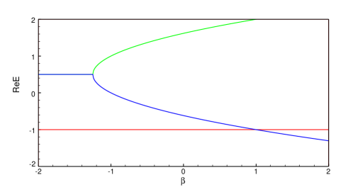
Figure 1: Real part of the eigenvalus

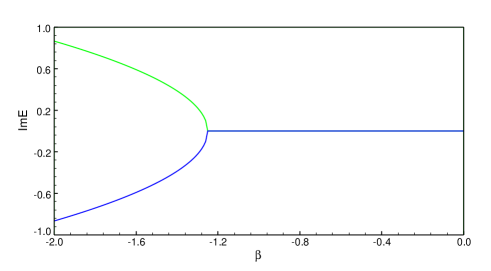
Figure 2: Imaginary part of the eigenvalues

References

[1] Cohen-Tannoudji C, Diu B, and Laloë F 1977 Quantum Mechanics (John Wiley & Sons, New York).
[2] Pilar F L 1968 Elementary Quantum Chemistry
(McGraw-Hill, New York).
[3] Hammermesh M 1962 Group Theory and its Application to
Physical Problems (Addison-Wesley, Reading, Massachussets).
[4] Cotton F A 1990 Chemical Applications of Group Theory
(John Wiley & Sons, New York).
[5] Bender C M 2005 Contemp. Phys.46 277.
[6] Bender C M 2007 Rep. Prog. Phys.70 947.
[7] Heiss W D and Sannino A L 1990 J. Phys. A23 1167.
[8] Heiss W D 2000 Phys. Rev. E61 929.
[9] Heiss W D and Harney H L 2001 Eur. Phys. J. D17 149.
[10] Heiss W D 2004 Czech. J. Phys.54 1091.
[11] Günther U, Rotter I, and Samsonov B F 2007 J.
Phys. A40 8815.
[12] Moiseyev N and Friedland S 1980 Phys. Rev. A22 618.
[13] Kato T 1995 Perturbation theory for linear operators
(Springer, Berlin Heidelberg).
[14] Bender C M, Brody D C, and Jones H F 2003 Am. J.
Phys.71 1095.
[15] Dolfo G and Vigué J 2018 Eur. J. Phys.39 025005.
[16] Fernández F M 2018 Eur. J. Phys.39
045005.
[17] Li B, Xu T, Liu J, and Li M 2020 Eur. J. Phys.41 025305.
[18] Berry M V and O’Dell D H J 1998 J. Phys. A31 2093.