Abstract

A new generalized ModMax model of nonlinear electrodynamics with four parameters is proposed. The ModMax model and Born–Infeld-type electrodynamics are particular cases of the present model. It is shown that a singularity of the electric field at the center of point-like charged particles is absent. We found corrections to Coulomb’s law at $r\rightarrow\infty$ and obtained the total electrostatic and magnetic energies of point-like charges. Free electric and magnetic charges and their densities are obtained.

Recently, a new model, named ModMax model, of nonlinear electrodynamics (NED) which is duality and conformal invariant, as well as Maxwell electrodynamics, was proposed in [1]. Some aspects of this model and its applications were studies in [2, 3, 4, 5, 6, 7]. Earlier proposals of conformal invariant NED was in [8, 9, 10, 11].

The duality-invariant conformal electrodynamics was introduced in [1] and it is described by the Lagrangian density

$$L=-{\cal F}\cosh(\gamma)+\sqrt{{\cal F}^{2}+{\cal G}^{2}}\sinh(\gamma),$$ (1)

where

$${\cal F}=\frac{1}{4}F_{\mu\nu}F^{\mu\nu}=\frac{1}{2}\left(\textbf{B}^{2}-\textbf{E}^{2}\right),~{}~{}~{}~{}{\cal G}=\frac{1}{4}F_{\mu\nu}\tilde{F}^{\mu\nu}=\textbf{B}\cdot\textbf{E},$$ (2)

are Lorentz invariants with B, E being the magnetic induction and electric fields correspondingly, $F_{\mu\nu}=\partial_{\mu}A_{\nu}-\partial_{\nu}A_{\mu}$, $\tilde{F}^{\mu\nu}=(1/2)\epsilon^{\mu\nu\alpha\beta}F_{\alpha\beta}$ is the dual electromagnetic field, and $\gamma$ is the dimensionless parameter. This model as well as Maxwell electrodynamics with the Lagrangian density ${\cal L}_{M}=-{\cal F}$ possess singularities in the centre of point-like charges. In addition, the electromagnetic energy of charges is infinite. To smooth singularities we propose the generalized ModMax model with the Lagrangian density

$${\cal L}=\frac{1}{\beta}\left(1-\left(1-\frac{\beta L}{\sigma}-\frac{\beta\lambda{\cal G}^{2}}{2\sigma}\right)^{\sigma}\right),$$ (3)

where $L$ is given by Eq. (1), $\beta$ and $\lambda$ have the dimensions of $(length)^{4}$ and $\sigma$ is the dimensionless parameter. At $\sigma=1$, $\lambda=0$ we come to ModMax model, when $\gamma=0$ one has the Born–Infeld-type model [12], [13], at $\sigma=1/2$, $\gamma=0$ we arrive at the generalized Born–Infeld model [14], and at $\sigma=1/2$, $\gamma=0$, $\lambda=\beta$ one comes to Born–Infeld model ($\beta=1/b^{2}$) [15]. At $\sigma\rightarrow\infty$ the Lagrangian density (3) becomes

$${\cal L}_{exp}=\frac{1}{\beta}\left(1-\exp\left(-\beta L-\beta\lambda{\cal G}^{2}/2\right)\right).$$ (4)

Some exponential NED models were considered in [16], [17]. Thus, our model (3) allows us to consider different NED by fixing the parameters introduced. The Born–Infeld model is of interest because at the low energy D-brain dynamics is governed by Born–Infeld-type action [18], [19]. Making use of the Taylor series, at $\beta L\ll 1$, $\beta\lambda{\cal G}^{2}\ll 1$, the Lagrangian density (3) becomes

$${\cal L}=L+\frac{\beta(1-\sigma)L^{2}}{2\sigma}+\frac{\lambda}{2}{\cal G}^{2}+{\cal O}(LG^{2})+{\cal O}(L^{3}).$$ (5)

As a result, in the weak-field limit and small $\gamma$ when the condition $\beta L\ll 1$ is satisfied, the Lagrangian density (3) approaches to the ModMax model. At $\gamma=0$ Eq. (5) corresponds to the Heisenberg–Euler-type electrodynamics [20].

Adding to Eq. (3) the source term $A_{\mu}j^{\mu}$ and varying the action we obtain the Euler–Lagrange equations

$$\partial_{\mu}\left({\cal L}_{\cal F}F^{\mu\nu}+{\cal L}_{\cal G}\tilde{F}^{\mu\nu}\right)=j^{\nu},$$ (6)

where

$${\cal L}_{\cal F}=\frac{\partial{\cal L}}{\partial{\cal F}}=\left(1-\frac{\beta L}{\sigma}-\frac{\beta\lambda{\cal G}^{2}}{2\sigma}\right)^{\sigma-1}L_{\cal F},~{}~{}~{}L_{\cal F}=-\cosh(\gamma)+\frac{{\cal F}\sinh(\gamma)}{\sqrt{{\cal F}^{2}+{\cal G}^{2}}},$$

$${\cal L}_{\cal G}=\frac{\partial{\cal L}}{\partial{\cal G}}=\left(1-\frac{\beta L}{\sigma}-\frac{\beta\lambda{\cal G}^{2}}{2\sigma}\right)^{\sigma-1}(L_{\cal G}+\lambda G),~{}~{}~{}L_{\cal G}=\frac{{\cal G}\sinh(\gamma)}{\sqrt{{\cal F}^{2}+{\cal G}^{2}}}.$$ (7)

Field equations (6) can be represented as Maxwell equations making use of definitions of the electric displacement and magnetic fields

$$\textbf{D}=\frac{\partial{\cal L}}{\partial\textbf{E}}=\varepsilon\textbf{E}+\nu\textbf{B},~{}~{}~{}\varepsilon=-{\cal L}_{\cal F},~{}\nu={\cal L}_{\cal G},$$

$$\textbf{H}=-\frac{\partial{\cal L}}{\partial\textbf{B}}=\mu^{-1}\textbf{B}-\nu\textbf{E},~{}~{}~{}\mu=\varepsilon^{-1}.$$ (8)

With help of Eq. (8) Euler–Lagrange equations (6) can be represented as Maxwell equations in Gaussian quantities

$$\nabla\cdot\textbf{D}=4\pi\rho,~{}~{}\frac{\partial\textbf{D}}{\partial t}-\nabla\times\textbf{H}=4\pi\textbf{j}.$$ (9)

Second pair of Maxwell equations follows from the Bianchi identity $\partial_{\mu}\tilde{F}^{\mu\nu}=0$,

$$\nabla\cdot\textbf{B}=0,~{}~{}\frac{\partial\textbf{B}}{\partial t}+\nabla\times\textbf{E}=0.$$ (10)

From Eq. (8) we obtain the relation

$$\textbf{D}\cdot\textbf{H}=(\varepsilon^{2}-\nu^{2}){\cal G}+2\varepsilon\nu{\cal F}.$$ (11)

According to the criterion of [21] the dual symmetry takes place if $\textbf{D}\cdot\textbf{H}=\textbf{E}\cdot\textbf{B}$. One can verify from Eq. (11) that the dual symmetry holds in two cases: $\sigma=1$, $\lambda=0$ which corresponds to ModMax model or for Born–Infeld-type model with $\sigma=1/2$, $\lambda=\beta$. It is worth noting that the two-parametric generalized Born–Infeld model ($\sigma=1/2$, $\lambda=\beta$) was considered and shown to be duality invariant in [4].

From Eq. (9), for the source of the point-like charged particle with the electric charge $q$, in Gaussian units, we obtain the equation as follows

$$\nabla\cdot\textbf{D}=4\pi q\delta(\textbf{r}),$$ (12)

with the solution

$$\textbf{D}=\frac{q\textbf{r}}{r^{3}}.$$ (13)

From Eqs. (8) and (13) one finds

$$E\exp(\gamma)\left(1-\frac{\beta E^{2}}{2\sigma}\exp(\gamma)\right)^{\sigma-1}=\frac{q}{r^{2}}.$$ (14)

Introducing the dimensionless variables

$$v=\frac{\sqrt{\beta}E}{\sqrt{2\sigma}}\exp\left(\frac{\gamma}{2}\right),~{}~{}~{}u=\frac{r\sqrt[4]{2\sigma}}{{\sqrt[4]{\beta}}\sqrt{q}}\exp\left(\frac{\gamma}{4}\right),$$ (15)

Eq. (14) takes the form

$$v\left(1-v^{2}\right)^{\sigma-1}=\frac{1}{u^{2}}.$$ (16)

It follows from Eq. (16) that at $u\rightarrow 0$, $v(0)=1$ for $\sigma<1$, or in terms of electric fields

$$E(0)=\sqrt{\frac{2\sigma}{\beta}}\exp\left(-\frac{\gamma}{2}\right).$$ (17)

Thus, the electric field of the point-like charged particle in the center is finite and possesses the maximum value for $\sigma<1$. When $\sigma$ increases the maximum value of electric fields increases, but if $\gamma$ increases the electric field in the center decreases. For the cases $\sigma=1/2$ (Born–Infeld-type model) and $\sigma=3/4$ exact solutions to Eq. (16) and their asymptotic as $u\rightarrow 0$ are

$$v=\frac{1}{\sqrt{1+u^{4}}},~{}~{}~{}~{}v=1-\frac{u^{4}}{2}+\frac{3u^{8}}{8}+{\cal O}(u^{12})~{}~{}~{}~{}\sigma=\frac{1}{2},$$

$$v=\frac{\sqrt{\sqrt{1+4u^{8}}-1}}{\sqrt{2}u^{4}},~{}~{}~{}~{}v=1-\frac{u^{8}}{2}+{\cal O}(u^{16})~{}~{}~{}~{}\sigma=\frac{3}{4}.$$ (18)

The plots of function $v(u)$ for $\sigma=1/4$, $\sigma=1/2$ and $\sigma=3/4$ are given in Fig. (1).

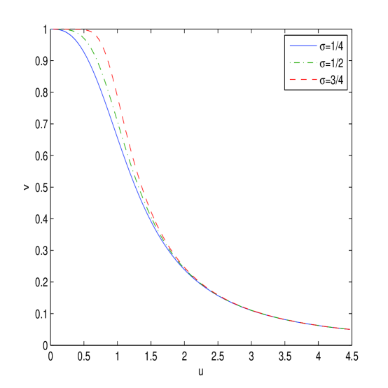
Figure 1: The plot of the function $v(u)$ for $\sigma=1/4$, $\sigma=1/2$ and $\sigma=3/4$.

In the general case for $\sigma<1$, the functions $v(u)$ as $u\rightarrow 0$ ($r\rightarrow 0$) and $u\rightarrow\infty$ ($r\rightarrow\infty$) become

$$v=1-\frac{u^{2/(1-\sigma)}}{2}+{\cal O}(u^{4/(1-\sigma)})~{}~{}~{}~{}u\rightarrow 0,$$

$$v=\frac{1}{u^{2}}-\frac{1-\sigma}{u^{6}}+{\cal O}(u^{-8})~{}~{}~{}~{}u\rightarrow\infty.$$ (19)

Making use of Eqs. (15) and (19) we obtain the asymptotic value of the electric field as $r\rightarrow 0$ and $r\rightarrow\infty$

$$E=\sqrt{\frac{2\sigma}{\beta}}\exp\left(-\frac{\gamma}{2}\right)-\frac{(2\sigma)^{(2-\sigma)/(2(1-\sigma))}r^{2/(1-\sigma)}}{2\beta^{(2-\sigma)/(2(1-\sigma))}q^{1/(1-\sigma)}}\exp\left(\frac{\gamma\sigma}{(2(1-\sigma)}\right)$$

$$+{\cal O}(r^{4/(1-\sigma))})~{}~{}~{}~{}~{}~{}r\rightarrow 0,$$

$$E=\frac{q}{r^{2}}\exp(-\gamma)-\frac{(1-\sigma)\beta q^{3}}{2\sigma r^{6}}\exp(-2\gamma)+{\cal O}(r^{-8})~{}~{}~{}~{}~{}~{}r\rightarrow\infty.$$ (20)

Equation (20) gives the correction to Coulomb’s law as $r\rightarrow\infty$. We have damping of the electric field because of parameter $\gamma$. Corrections to Coulomb’s law for the case of Born–Infeld-type electrodynamics ($\sigma=1/2$) and exponential-like electrodynamics (4) ($\sigma=\infty$) are similar but with the opposite sign. At $\sigma=1$, $\lambda=0$, $\gamma=0$, one has Maxwell’s electrodynamics and we come to the Coulomb law $E=q/r^{2}$ as $r\rightarrow\infty$, but the electric field at the origin is infinite.

The energy-momentum tensor is given by

$$T_{\mu\nu}=F_{\mu\alpha}\left({\cal L}_{\cal F}F_{~{}\nu}^{\alpha}+{\cal L}_{\cal G}\tilde{F}_{~{}\nu}^{\alpha}\right)-g_{\mu\nu}{\cal L}.$$ (21)

From Eq. (21) we obtain the energy density

$$T_{0}^{~{}0}=-E^{2}{\cal L}_{\cal F}-G{\cal L}_{\cal G}-{\cal L}.$$ (22)

In the case of pure electric field ($\textbf{B}=0$) the energy density (22) becomes

$$T_{0}^{~{}0}=E^{2}e^{\gamma}\left(1-\frac{\beta E^{2}}{2\sigma}e^{\gamma}\right)^{\sigma-1}-\frac{1}{\beta}\left(1-\left(1-\frac{\beta E^{2}}{2\sigma}e^{\gamma}\right)^{\sigma}\right).$$ (23)

For the Born–Infeld-type electrodynamics with $\sigma=1/2$ we can calculate the total electrostatics energy of point-like charged particles. Introducing the dimensionless variables

$$y=\beta E^{2}\exp(\gamma),~{}~{}~{}~{}x=\frac{r^{2}\exp(\gamma/2)}{q\sqrt{\beta}},$$ (24)

we obtain from Eq. (14) equation

$$y=\frac{1}{1+x^{2}}.$$ (25)

Then, making use of Eqs. (23), (24) and (25), the total electrostatics energy of point-like charged particles (for $\sigma=1/2$) is given by

$${\cal E}=4\pi\int_{0}^{\infty}T_{0}^{~{}0}r^{2}dr=\frac{2\pi q^{3/2}\exp(-3\gamma/4)}{\beta^{1/4}}I,$$

$$I=\int_{0}^{\infty}\left(\frac{\sqrt{1+x^{2}}}{\sqrt{x}}-\sqrt{x}\right)dx=-\frac{2}{3}\sqrt{x}\left(x-3{{}_{2}}F_{1}\left(-\frac{1}{2},\frac{1}{4};\frac{5}{4};-x^{2}\right)\right)_{0}^{\infty}.$$ (26)

Taking into account the asymptotic of hypergeometric function ${}_{2}F_{1}(-1/2,1/4;5/4;-x^{2})$ we obtain the total electrostatics energy of point-like charged particles

$${\cal E}\approx 15.5327\frac{q^{3/2}}{\beta^{1/4}}\exp\left(-\frac{3\gamma}{4}\right).$$ (27)

For Born–Infeld electrodynamics ($\beta=1/b^{2}$) at $\gamma=0$ we come to the result obtained in [15].

To study the conformal invariance of the proposed model (3), we calculate the trace of the energy-momentum tensor $T_{\mu}^{~{}\mu}$. According to [22], the conformal invariance takes place if $T_{\mu}^{~{}\mu}=0$. From Eqs. (7) and (27) we obtain

$$T_{\mu}^{~{}\mu}=4\left({\cal F}{\cal L}_{\cal F}+{\cal G}{\cal L}_{\cal G}-{\cal L}\right)$$

$$=4\left(1-\frac{\beta L}{\sigma}-\frac{\beta\lambda{\cal G}^{2}}{2\sigma}\right)^{\sigma-1}\left(\frac{(\sigma-1)L}{\sigma}+\frac{(2\sigma-1)\lambda G^{2}}{2\sigma}+\frac{1}{\beta}\right)-\frac{4}{\beta}.$$ (28)

Equation (28) shows that the conformal invariance ($T_{\mu}^{~{}\mu}=0$) holds only for $\sigma=1$, $\lambda=0$ corresponding to the ModMax model.

In accordance with [15] we introduce the “free charge density” $\rho_{free}$ by the equation

$$\nabla\cdot E=\frac{1}{r^{2}}\frac{d}{dr}(r^{2}E)=4\pi\rho_{free},$$ (29)

where $E$ obeys Eq. (14). To calculate the distribution of the free charge one has to obtain $\rho_{free}$ from Eq. (29). We have exact solutions to Eq. (14) for $\sigma=1/2$ and $\sigma=3/4$. Making use of Eq. (15), from Eq. (18) we find

$$E=\frac{q\exp(-\gamma/2)}{r_{0}^{2}\sqrt{1+(r/r_{0})^{4}\exp(\gamma)}}~{}~{}~{}~{}~{}~{}~{}~{}\sigma=\frac{1}{2},$$

$$E=\frac{qr_{0}^{2}\exp(-3\gamma/2)\sqrt{\sqrt{1+(9r^{8}/r_{0}^{8})\exp(2\gamma)}-1}}{\sqrt{3}r^{4}}~{}~{}~{}~{}~{}~{}~{}~{}\sigma=\frac{3}{4},$$ (30)

where $r_{0}=\sqrt[4]{\beta}\sqrt{q}$. When $q$ is the charge of the electron, $r_{0}$ is the electron radius [15]. It follows from Eq. (30) that for $r\rightarrow\infty$ the electric field $E\rightarrow(q/r^{2})\exp(-\gamma)$ and for $r\rightarrow 0$ we have

$$E\rightarrow\frac{1}{\sqrt{\beta}}\exp\left(-\frac{\gamma}{2}\right)~{}~{}~{}~{}~{}~{}~{}~{}~{}\sigma=\frac{1}{2},$$

$$E\rightarrow\sqrt{\frac{3}{2\beta}}\exp\left(-\frac{\gamma}{2}\right)~{}~{}~{}~{}~{}~{}~{}~{}~{}\sigma=\frac{3}{4},$$ (31)

according to Eq. (20). From Eqs. (29) and (30) we obtain “free charge density”

$$\rho_{free}=\frac{q\exp(-\gamma/2)}{2\pi r_{0}^{2}r(1+(r/r_{0})^{4}\exp(\gamma))^{3/2}}~{}~{}~{}~{}~{}~{}~{}~{}~{}\sigma=\frac{1}{2},$$

$$\rho_{free}=\frac{qr_{0}^{2}\exp(-3\gamma/2)}{2\sqrt{3}\pi r^{5}}\sqrt{\frac{\sqrt{1+(9r^{8}/r_{0}^{8})\exp(2\gamma)}-1}{1+(9r^{8}/r_{0}^{8})\exp(2\gamma)}}~{}~{}~{}~{}~{}~{}~{}~{}~{}\sigma=\frac{3}{4},$$ (32)

For Born–Infeld electrodynamics, in the case $\sigma=1/2$, $\gamma=0$, one comes from Eq. (32) to the result found in [15]. Now we can calculate free charges

$$q_{free}=4\pi\int_{0}^{\infty}r^{2}\rho_{free}dr=\left(r^{2}E^{2}\right)_{0}^{\infty}.$$ (33)

Making use of Eqs. (20) and (33) we find the free charge for any parameter $\sigma$

$$q_{free}=q\exp(-\gamma).$$ (34)

Equation (34) shows that the free charge is less from $q$ by the factor $\exp(-\gamma)$. From Eq. (30) we obtain the free electric charges, in the cases $\sigma=1/2$ and $\sigma=3/4$, inside the sphere $r<r_{0}$

$$q_{free}(r_{0})=4\pi\int_{0}^{r_{0}}r^{2}\rho_{free}dr=\left(r^{2}E\right)_{0}^{r_{0}}=q_{free}\frac{\exp(\gamma/2)}{\sqrt{1+\exp(\gamma)}}~{}~{}~{}~{}~{}\sigma=1/2,$$

$$q_{free}(r_{0})=q_{free}\frac{\sqrt{\sqrt{(1+9\exp(2\gamma)}-1}}{\sqrt{3}}\exp\left(-\frac{\gamma}{2}\right)~{}~{}~{}~{}~{}~{}~{}~{}~{}~{}~{}~{}~{}\sigma=3/4$$ (35)

The plots of the functions $q_{free}(r_{0})/q_{free}$ versus $\gamma$ is presented in Fig. 2.

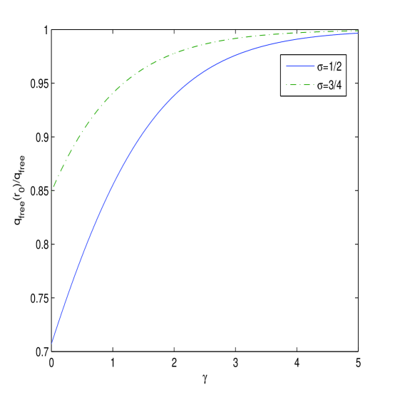
Figure 2: The plot of the functions $q_{free}(r_{0})/q_{free}$ versus $\gamma$ for $\sigma=1/2$ and $\sigma=3/4$.

It follows from Eq. (35) and the Fig. 2 that at $\gamma=0$ $q_{free}(r_{0})/q_{free}\approx 0.71$ for $\sigma=1/2$ and $q_{free}(r_{0})/q_{free}\approx 0.85$ for $\sigma=3/4$. Therefore, $71\%$ of the electron charge $q_{free}$ is contained in the electron radius sphere for $\sigma=1/2$ and $85\%$ of the electron charge is concentrated within the electron radius for $\sigma=3/4$. When parameter $\gamma$ increases more charge is inside the electron radius sphere.

For the magnetic monopole we have equation

$$\nabla\cdot\textbf{B}=4\pi Q\delta(\textbf{r}),$$ (36)

where $Q$ is the magnetic charge. For a magnetic monopole we have equation

$$B=\frac{Q}{r^{2}}.$$ (37)

From Eq. (22) we obtain the magnetic energy density ($E=0$) of the magnetic monopole

$$T_{0}^{~{}0}=-{\cal L}=\frac{1}{\beta}\left(\left(1+\frac{\beta Q^{2}}{2\sigma r^{4}}e^{-\gamma}\right)^{\sigma}-1\right).$$ (38)

The total magnetic energy is given by

$${\cal E}_{m}=4\pi\int_{0}^{\infty}T_{0}^{~{}0}r^{2}dr=-\frac{4\pi}{\beta}\int_{0}^{\infty}r^{2}\left(1-\left(1+\frac{\beta Q^{2}}{2\sigma r^{4}}e^{-\gamma}\right)^{\sigma}\right)dr$$ (39)

Integral (39) converges for $0<\sigma<1$ and the energy of the magnetic monopole is finite within our model. In Table 1 we present the approximate values of the dimensionless energy $\bar{\cal E}_{m}=\beta^{1/4}Q^{-3/2}\exp(3\gamma/4){\cal E}_{m}$ for $\sigma=0.1,0.2,..,0.7$.

Table 1: The dimensionless energy $\bar{{\cal E}}_{m}$

$\sigma$	0.1	0.2	0.3	0.4	0.5	0.6	0.7
$\bar{\cal E}_{m}$	6.58	8.38	10.13	12.28	15.45	22.29	58.78

Table 1 shows that with increasing parameter $\sigma$ the magnetic energy of the monopole increasing. When parameter $\gamma$ increases the magnetic energy ${\cal E}_{m}$ decreases.

From Eq. (8) we obtain the magnetic field of the monopole

$$\textbf{H}=\frac{Q}{r^{2}}e^{-\gamma}\left(1+\frac{\beta Q^{2}}{2\sigma r^{4}}e^{-\gamma}\right)^{\sigma-1}.$$ (40)

The “free magnetic charge density” $\eta_{free}$ is defined by the equation

$$\nabla\cdot H=\frac{1}{r^{2}}\frac{d}{dr}(r^{2}H)=4\pi\eta_{free}.$$ (41)

Making use of Eq. (41) one finds from Eq. (40) the “free magnetic charge density”

$$\eta_{free}=-\frac{\beta Q^{3}(\sigma-1)}{2\pi\sigma r^{7}}e^{-2\gamma}\left(1+\frac{\beta Q^{2}}{2\sigma r^{4}}e^{-\gamma}\right)^{\sigma-2}.$$ (42)

Similar to Eq. (33) we obtain, by using Eq. (40), the free magnetic charge

$$Q_{free}=\frac{1}{4\pi}\int\nabla\cdot Hd^{3}x=\int_{0}^{\infty}\frac{d}{dr}(r^{2}H)dr=\left(r^{2}H^{2}\right)_{0}^{\infty}=Q\exp(-\gamma).$$ (43)

Thus, the equation for the free magnetic charge is similar to the free electric charge (34). From Eq. (40), one finds the free magnetic charge inside the sphere of the radius $r_{m}=\beta^{1/4}\sqrt{Q}$

$$Q_{free}(r_{m})=\left(r^{2}H\right)_{0}^{r_{0}}=Q_{free}\left(1+\frac{1}{2\sigma}e^{-\gamma}\right)^{\sigma-1}.$$ (44)

The plots of the functions $Q_{free}(r_{m})/Q_{free}$ versus $\gamma$ for $\sigma=1/8$, $\sigma=1/2$ and $\sigma=3/4$ is presented in Fig. 3.

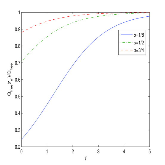
Figure 3: The plot of the functions $Q_{free}(r_{m})/Q_{free}$ versus $\gamma$ for $\sigma=1/8$, $\sigma=1/2$ and $\sigma=3/4$.

According to Eq. (44) $(1+e^{-\gamma}/(2\sigma))^{\sigma-1}$ of the magnetic charge $Q_{free}$ is inside the sphere of the radius $r_{m}$. The plot of the function $Q_{free}(r_{m})/Q_{free}$ is in Fig. 4.

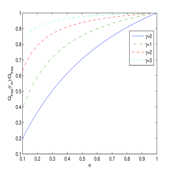
Figure 4: The plot of the functions $Q_{free}(r_{m})/Q_{free}$ versus $\sigma$, for $\gamma=0,1,2,3$.

Figure 4 shows that the ratio $Q_{free}(r_{m})/Q_{free}$ increases with increasing parameters $\sigma$ and $\gamma$. As a result, more magnetic charge is concentrated in the sphere of the radius $r_{m}$ with greater values of $\sigma$ and $\gamma$.

The generalised ModMax model proposed as compared to ModMax model (1) possesses the attractive features as follows.

$\bullet$ At some parameters $\beta$, $\lambda$, $\gamma$ and $\sigma$ we come to different models (including the Born–Infeld electrodynamics) discussed in the literature.

$\bullet$ In the weak-field limit and $\gamma=0$, the Lagrangian density leads to the Heisenberg–Euler electrodynamics.

$\bullet$ The electric field of the point-like charged particle in the origin is finite and possesses the maximum value (for $\sigma<1$).

$\bullet$ The electric and magnetic energies of point-like charged particles is finite for some parameters $\sigma$.

Such properties take place also for the two-parametric duality invariant generalization of Born–Infeld electrodynamics found in [1], [4].

In addition, we calculated the free electric and magnetic densities in our model that allow us to study the distributes of the electric and magnetic charges in the space.

References

[1] I. Bandos, K. Lechner, D. Sorokin, and P. Townsend, Phys. Rev. D 102, (2020) 121703; arXiv:2007.09092 [hep-th].
[2] B. P. Kosyakov, Phys. Lett. B 810, 135840 (2020); arXiv:2007.13878 [hep-th].
[3]Z. Amirabi, S. Habib Mazharimousavi, Eur. Phys. J. C 81, 207 (2021); arXiv:2012.07443 [gr-qc].
[4]I. Bandos, , K. Lechner, D. Sorokin, and P. K. Townsend, JHEP 03, 022 (2021); arXiv:2012.09286 [hep-th].
[5] I. Bandos, K. Lechner, D. Sorokin, and P. Townsend, ModMax meets Susy, arXiv:2106.07547 [hep-th].
[6]D. Flores-Alfonso, B. A. Gonzalez-Morales, R. Linares, and M. Maceda, Phys. Lett. B 812, 136011 (2021); arXiv:2011.10836 [gr-qc].
[7]A. Ballon Bordo, D. Kubiznak, and T. R. Perche, Phys. Lett. B 817, 136312 (2021); arXiv:2011.13398 [hep-th].
[8] J. A. R. Cembranos, A. de la Cruz-Dombriz and J. Jarillo, JCAP 02, 042 (2015); arXiv:1407.4383 [gr-qc].
[9]J. A. R. Cembranos, A. de la Cruz-Dombriz and J. Jarillo, Universe 1, 412 (2015).
[10] V. I. Denisov, E. E. Dolgaya and V. A. Sokolov, Phys. Rev. D 96, 036008 (2017).
[11] I. P. Denisova, B. D. Garmaev, V. A. Sokolov, Eur. Phys. J. C 79, 531 (2019).
[12]S. I. Kruglov, Mod. Phys. Lett. A 32 (2017) 36, 1750201; arXiv:1612.04195 [physics.gen-ph].
[13] S. I. Kruglov, Ann. Phys. 383 (2017) 550; arXiv:1707.04495 [gr-qc].
[14] S. I. Kruglov, J. Phys. A 43 (2010) 375402; arXiv:0909.1032 [hep-th].
[15] M. Born and L. Infeld, Nature 132 (1933) 1004; Proc.
Roy. Soc. London A 144 (1934) 425-451.
[16] S. H. Hendi, JHEP 03, 065 (2012); arXiv:1405.5359 [gr-qc].
[17]S. I. Kruglov, Int. J. Mod. Phys. A 31, 1650058 (2016); arXiv:1607.03923 [gr-qc] .
[18] E. S. Fradkin and A. A. Tseytlin, Phys. Lett. B 163, 123 (1985).
[19] A. A. Tseytlin, Nucl. Phys. B 276, 391 (1985).
[20]S. I. Kruglov, Phys. Rev. D 75, 117301 (2007).
[21]G. W. Gibbons and D. Rasheed, Nucl. Phys. B 454 (1995) 185; arXiv:hep-th/9506035.