Abstract

In a recent paper we have a shown that the flattening of galactic rotation curves can be explained by retardation. However, this will rely on a temporal change of galactic mass. In our previous work we have kept only second order terms of the retardation time in our analysis, while higher terms in the Taylor expansion where not considered. Here we consider analysis to all orders and show that indeed a second order analysis will suffice, and higher order terms can be neglected.

xx 1 0 Received: ; Accepted: ; Published: date Effects of Higher Order Retarded Gravity Asher Yahalom ^1,2 Asher Yahalom

1 Introduction

Einstein’s general relativity (GR) is known to be invariant under general coordinate modifications. This group of general transformations has a Lorentz subgroup, which is valid even in the weak field approximation. This is seen through the field equations containing the d’Alembert (wave) operator, which can be solved using a retarded potential solution.

It is known that GR is verified by many types of observations. However, currently, Newton–Eins-
tein gravitational theory is at a crossroads. It has much in its favor observationally, and it has some very disquieting challenges. The successes that it has achieved in both astrophysical and cosmological scales have to be considered in light of the fact that GR needs to appeal to two unconfirmed ingredients, dark matter and energy, to achieve these successes. Dark matter has not only been with us since the 1920s (when it was initially known as the missing mass problem), but it has also become severe as more and more of it had to be introduced on larger distance scales as new data have become available. Here we will be particularly concerned in the excess dark matter needed to justify observed gravitational lensing. Moreover, 40-year-underground and accelerator searches and experiments have failed to establish its existence. The dark matter situation has become even more disturbing in recent years as the Large Hadron Collider was unable to find any super symmetric particle candidates, the community’s preferred form of dark matter.

While things may still take turn in favor of the dark matter hypothesis, the current situation is serious enough to consider the possibility that the popular paradigm might need to be amended in some way if not replaced altogether. The present paper seeks such a modification. Unlike other ideas such as Milgrom’s MOND Mond , Bekenstein’s TeVeS Bekenstein , Mannheim’s Conformal Gravity Mannheim0 ; Mannheim1 ; Mannheim2 , Moffat’s MOG MOG or $f(R)$ theories and scalar-tensor gravity Corda , the present approach is, the minimalist one adhering to the razor of Occam. It suggests to replace dark matter by effects within standard GR.

Dynamics of large scale structures is inconsistent with Newtonian mechanics. This was notified in the 1930’s by Fritz Zwicky zwicky , who pointed out that if more (unseen) mass would be present one would be able to solve the apparent contradiction. The phenomena was also observed in galaxies by Volders volders who have shown that star trajectories near the rim of galaxies do not move according to Newtonian predictions, and later corroborated by Rubin and Ford rubin1 ; rubin2 ; Binney for spiral galaxies.

In as series of papers we have shown that those discrepancies can be shown to result from retarded gravity as dictated by the theory of general relativity YaRe1 ; ge ; YaRe2 ; YahalomSym ; Wagman ; YaRe3 . Indeed in the absence of temporal density changes, retardation does not effect the gravitational force. However, density is not constant for galaxies, in fact there are many processes that change the mass density in galaxies over time. Mass accretion from the intergalactic medium and internal processes such as super novae leading to super winds Wagman modify the density. In addition to those local processes there is a cosmological decrease of density due to the cosmic expansion. However, the later process is many orders of magnitude smaller than the former.

In previous analysis YaRe1 ; ge ; YaRe2 ; YahalomSym ; Wagman ; YaRe3 the corrected gravitational force was evaluated assuming a second order approximation in the retardation time $\frac{R}{c}$, neglecting higher order terms without justification. Here we take into account all orders and show that a second order approximation is indeed sufficient.

2 Linear GR

Only in cases of extreme compact objects (black holes and neutron stars) and the very early universe we consider the solution of the full non-linear Einstein Equations YaRe1 . In most cases of astronomical interest (including the galactic case) a linear approximation to those equations around the flat Lorentz metric $\eta_{{\mu\nu}}$ is used, such that:

$$g_{{\mu\nu}}=\eta_{{\mu\nu}}+h_{{\mu\nu}},\quad\eta_{{\mu\nu}}\equiv\ {\rm diag}\ (1,-1,-1,-1),\qquad|h_{{\mu\nu}}|\ll 1$$ (1)

One then defines the quantity:

$$\bar{h}_{\mu\nu}\equiv h_{\mu\nu}-\frac{1}{2}\eta_{\mu\nu}h,\quad h=\eta^{{\mu\nu}}h_{{\mu\nu}},$$ (2)

$\bar{h}_{\mu\nu}=h_{\mu\nu}$ for non diagonal terms. For diagonal terms:

$$\bar{h}=-h\Rightarrow h_{\mu\nu}=\bar{h}_{\mu\nu}-\frac{1}{2}\eta_{\mu\nu}\bar{h}.$$ (3)

It was shown (Narlikar page 75, exercise 37, see also Edd ; Weinberg ; MTW ) that for a proper gauge the Einstein equations are:

$$\Box{\bar{h}}_{{\mu\nu}}\equiv{\bar{h}}_{{\mu\nu},\alpha}{}^{\alpha}=-\frac{16\pi G}{c^{4}}T_{\mu\nu},\qquad{\bar{h}}_{\mu\alpha,}{}^{\alpha}=0.$$ (4)

Equation (4) can be solved such that padma ; Carroll :

$${\bar{h}}_{{\mu\nu}}(\vec{x},t)=-\frac{4G}{c^{4}}\int\frac{T_{\mu\nu}(\vec{x}^{\prime},t-\frac{R}{c})}{R}d^{3}x^{\prime},$$

$$t \equiv \frac{x^{0}}{c},\quad\vec{x}\equiv x^{a}\quad a,b\in[1,2,3],$$

$$\vec{R} \equiv \vec{x}-\vec{x}^{\prime},\quad R=|\vec{R}|.$$ (5)

In Yahalom ; Yahalomb ; Yahalomc ; Yahalomd we explain why the symmetry between space and time is broken, which justifies the use of different notations for space and time. $\frac{4G}{c^{4}}\simeq 3.3\times 10^{-44}$; is a tiny number, hence, in the above calculation one can take $T_{\mu\nu}$, to zeroth order in $h_{\alpha\beta}$.We underline that the term $\frac{R}{c}$ is not the actual delay time between an arbitrarily moving source and arbitrarily moving observer and can only interpreted in this way if both are static, nevertheless equation (5) is an exact solution of equation (4). The reader who is interested in the actual delay time is invite to read Scott ; Will . We now evaluate the affine connection in the linear approximation:

$$\Gamma^{\alpha}_{\mu\nu}=\frac{1}{2}\eta^{\alpha\beta}\left(h_{\beta\mu,\nu}+h_{\beta\nu,\mu}-h_{{\mu\nu},\beta}\right).$$ (6)

Notice that the affine connection has first order terms in $h_{\alpha\beta}$; hence, to the first order $\Gamma^{\alpha}_{\mu\nu}u^{\mu}u^{\nu}$ appearing in the geodesic equation, $u^{\mu}u^{\nu}$ must be taken to zeroth order. In which:

$$u^{0}=\frac{1}{\sqrt{1-\frac{v^{2}}{c^{2}}}},u^{a}=\vec{u}=\frac{\frac{\vec{v}}{c}}{\sqrt{1-\frac{v^{2}}{c^{2}}}},\vec{v}\equiv\frac{d\vec{x}}{dt},\quad v=|\vec{v}|.$$ (7)

For velocities much smaller than the speed of light in vacuum:

$$u^{0}\simeq 1,\qquad\vec{u}\simeq\frac{\vec{v}}{c},\qquad u^{a}\ll u^{0}\qquad{\rm for}\quad v\ll c.$$ (8)

Hence, the current paper does not discuss the post-Newtonian approximation, in which matter travels at speeds close to the speed of light, but  we do consider the retardation effects which are due to the finite propagation speed of the gravitational field. We emphasize that assuming $\frac{v}{c}<<1$ is not the same as stating $\frac{R}{c}<<1$ (with $R$ being the typical size of a galaxy) since:

$$\frac{R}{c}=\frac{v}{c}\frac{R}{v}$$ (9)

now since in galaxies, $\frac{R}{v}$ is huge ($\frac{R}{v}\simeq 10^{15}$ seconds); it follows that, $\frac{v}{c}$ can be dismissed but not $\frac{R}{c}$, for which $\frac{R}{c}\simeq 10^{12}$ seconds. Inserting Equations (6) and (8) in the geodesic equation, we arrive at the approximate equation:

$$\frac{dv^{a}}{dt}\simeq-c^{2}\Gamma^{a}_{00}=-c^{2}\left(h^{a}_{0,0}-\frac{1}{2}h_{00,}{}^{a}\right)$$ (10)

Taking a standard matter $T_{\mu\nu}$, assuming $\rho c^{2}\gg p$ and, taking into account Equation (8), we arrive at $T_{00}=\rho c^{2}$, while the remaining tensor components are much smaller. Therefore, $\bar{h}_{00}$ is larger than other components of $\bar{h}_{\mu\nu}$. Notice that it is not possible to deduce from the magnitudes of quantities that a similar difference exists between the derivatives of those quantities. Gauge conditions in Equation (4) lead to:

$$\bar{h}_{\alpha 0,}{}^{0}=-\bar{h}_{\alpha a,}{}^{a}\qquad\Rightarrow\bar{h}_{00,}{}^{0}=-\bar{h}_{0a,}{}^{a},\quad\bar{h}_{b0,}{}^{0}=-\bar{h}_{ba,}{}^{a}.$$ (11)

Thus, the zeroth derivative of $\bar{h}_{00}$ (which contains a $\frac{1}{c}$) is of similar order as the spatial derivative of $\bar{h}_{0a}$. Also the zeroth derivative of $\bar{h}_{0a}$ (see equation (10)) is of similar order as the spatial derivative of $\bar{h}_{ab}$. However, we can compare spatial derivatives of $\bar{h}_{00}$ and $\bar{h}_{ab}$ and conclude that the former is larger. Taking into account equation (3) and the above consideration, we write equation (10) as:

$$\frac{dv^{a}}{dt}\simeq\frac{c^{2}}{4}\bar{h}_{00,}{}^{a}\Rightarrow\frac{d\vec{v}}{dt}=-\vec{\nabla}\phi=\vec{F},\qquad\phi\equiv\frac{c^{2}}{4}\bar{h}_{00}$$ (12)

Thus, the gravitational potential $\phi$ can be estimated using Equation (5):

$$\phi = \frac{c^{2}}{4}\bar{h}_{00}=-\frac{G}{c^{2}}\int\frac{T_{00}(\vec{x}^{\prime},t-\frac{R}{c})}{R}d^{3}x^{\prime}$$ (13)

$$= -G\int\frac{\rho(\vec{x}^{\prime},t-\frac{R}{c})}{R}d^{3}x^{\prime}$$

and $\vec{F}$ is the force per unit mass. In the case that the mass density $\rho$ does not depend on time, we may use the Newtonian instantaneous action at a distance. Notice, however, that it is improbable that $\rho$ is static for a galaxy, as it accretes intergalactic medium gas. Also notice that the velocity of galactic and intergalactic matter components (stars, dust & gas) are implicit in the above formulation as the a time dependent density requires a velocity field according to the continuity equation (52) of YahalomSym .

Inserting equation (13) into equation (12) will lead to:

$$\vec{F} = \vec{F}_{Nr}+\vec{F}_{r}$$

$$\vec{F}_{Nr} = -G\int\frac{\rho(\vec{x}^{\prime},t-\frac{R}{c})}{R^{2}}\hat{R}d^{3}x^{\prime},\qquad\hat{R}\equiv\frac{\vec{R}}{R}$$

$$\vec{F}_{r} \equiv -\frac{G}{c}\int\frac{\rho^{(1)}(\vec{x}^{\prime},t-\frac{R}{c})}{R}\hat{R}d^{3}x^{\prime},\qquad\rho^{(n)}\equiv\frac{\partial^{n}\rho}{\partial t^{n}}.$$ (14)

Thus a retarded potential does not only imply a retarded Newtonian force $\vec{F}_{Nr}$, but in addition a pure "retardation" force $\vec{F}_{r}$ which decreases slowly than the Newtonian force with distance, explaining the peculiar form of the galactic rotation curves. We emphasize that this result is independent of any perturbation expansion in the delay time $\frac{R}{c}$ as was done in YahalomSym . However, the perturbation expansion does shed some light on the nature of those force terms as will be explained in the next section.

3 Retardation Effects Beyond the Newtonian Approximation

The duration $\frac{R}{c}$ may be tens of thousands of years, but may be short with respect to the duration in which the galactic density changes considerably. Thus, we write a Taylor series for the density:

$$\rho(\vec{x}^{\prime},t-\frac{R}{c})=\sum_{n=0}^{\infty}\frac{1}{n!}\rho^{(n)}(\vec{x}^{\prime},t)(-\frac{R}{c})^{n}.$$ (15)

By inserting Equations (15) into Equation (13), we will obtain:

$$\phi = \phi_{2}+\phi_{(n>2)}$$

$$\phi_{2} = -G\int\frac{\rho(\vec{x}^{\prime},t)}{R}d^{3}x^{\prime}+\frac{G}{c}\int\rho^{(1)}(\vec{x}^{\prime},t)d^{3}x^{\prime}-\frac{G}{2c^{2}}\int R\rho^{(2)}(\vec{x}^{\prime},t)d^{3}x^{\prime}$$

$$\phi_{(n>2)} = -G\sum_{n=3}^{\infty}\frac{(-1)^{n}}{n!c^{n}}\int R^{n-1}\rho^{(n)}(\vec{x}^{\prime},t)d^{3}x^{\prime}$$ (16)

The Newtonian potential is the first term, the second term has null contribution, and the third term is the lower order correction to the Newtonian theory:

$$\phi_{r}=-\frac{G}{2c^{2}}\int R\rho^{(2)}(\vec{x}^{\prime},t)d^{3}x^{\prime}$$ (17)

The expansion given in Equation (16), being a Taylor series expansion, is only valid for limited radii determined by the convergence of the infinite sum:

$$R<c\ T_{max}\equiv R_{max}$$ (18)

hence the current approximation can only be used in the near field regime, this is to be contrasted with the far field approximation used for gravitational radiation Einstein2 ; Taylor ; Castelvecchi . The restriction is even more severe when one uses a second order expansion as was done in YahalomSym .

If $n>2$ terms can be neglected the total force per unit mass can be approximated as:

$$\vec{F} \simeq \vec{F}_{N}+\vec{F}_{ar}$$

$$\vec{F}_{N} = -\vec{\nabla}\phi_{N}=-G\int\frac{\rho(\vec{x}^{\prime},t)}{R^{2}}\hat{R}d^{3}x^{\prime},\qquad\hat{R}\equiv\frac{\vec{R}}{R}$$

$$\vec{F}_{ar} \equiv -\vec{\nabla}\phi_{r}=\frac{G}{2c^{2}}\int\rho^{(2)}(\vec{x}^{\prime},t)\hat{R}d^{3}x^{\prime}.$$ (19)

In the above $\vec{F}_{N}$ is a non retarded Newtonian force. To see how this comes about from the existence of a Newtonian retarded force and retardation force as defined in equation (14) we write those expressions up to order $O(1/c^{2})$ using equation (15), we thus have:

$$\vec{F}_{Nr} \simeq -G\int\frac{\rho(\vec{x}^{\prime},t)}{R^{2}}\hat{R}d^{3}x^{\prime}+\frac{G}{c}\int\frac{\rho^{(1)}(\vec{x}^{\prime},t)}{R}\hat{R}d^{3}x^{\prime}-\frac{G}{2c^{2}}\int\rho^{(2)}(\vec{x}^{\prime},t)\hat{R}d^{3}x^{\prime},$$

$$\vec{F}_{r} \simeq -\frac{G}{c}\int\frac{\rho^{(1)}(\vec{x}^{\prime},t)}{R}\hat{R}d^{3}x^{\prime}+\frac{G}{c^{2}}\int\rho^{(2)}(\vec{x}^{\prime},t)\hat{R}d^{3}x^{\prime}.$$ (20)

Adding those two terms we see that the first order terms in $\frac{1}{c}$ cancel and we are left with the zeroth and second order terms which only partially cancel, as detailed in equation (19). The cancellation of first order terms is indeed remarkable as was pointed out by Feynman Feynman with respect to the electromagnetic case.

$\vec{F}_{N}$ first introduced by Newton is attractive, however, the retardation force $\vec{F}_{r}$ can be either attractive or repulsive. Newtonian force decreases as $\frac{1}{R^{2}}$, however,  the retardation force doe not depend on distance as long as the Taylor approximation given in Equation (15) holds. Below a certain distance, the Newtonian force dominates, but for larger distances the retardation force has the upper hand. Newtonian force can be neglected for distances significantly larger compared to the retardation distance:

$$R\gg R_{r}\equiv c\Delta t$$ (21)

$\Delta t$ is a duration associated with the second order derivative of the density $\rho$. For $R\ll R_{r}$, retardation can be neglected and only Newtonian forces need to be considered; this is the situation in the solar system. As the galaxy accretes intergalactic gas, the galactic mass becomes larger thus $\dot{M}>0$; however, the intergalactic gas is depleted, and thus the rate at which the mass is accreted decreases resulting in $\ddot{M}<0$, hence we have an attractive retardation force.

One may claim that since for the galaxy $\ddot{M}<0$ and the total mass is conserved it must be that $\ddot{M}>0$ for the matter outside the galaxy and thus retardation forces $\vec{F}_{ar}$ inside and outside the galaxy should cancel out. This derivation, however, is false because equation (19) is only valid when $\frac{R}{c}$ is small, it is certainly not small if the rest of the universe outside the galaxy is taken into account. We shall later show by a detailed model that a retardation force exist regardless if one assumes the expansion of equation (15) or not.

As a final comment to this section please notice that if we introduce dimensionless quantities using suitable dimensional constants, such that:

$$\tilde{\rho}\equiv\frac{\rho}{\rho_{c}},\quad\tilde{x}\equiv\frac{\vec{x}}{R_{s}},\quad\bar{t}=\frac{t}{\Delta t}$$ (22)

and define $\Lambda$ such that:

$$\Lambda=\int\tilde{\rho}d^{3}\tilde{x}$$ (23)

we obtain that:

$$M=\int\rho d^{3}x=\rho_{c}R_{s}^{3}\int\tilde{\rho}d^{3}\tilde{x}=\Lambda\rho_{c}R_{s}^{3}.$$ (24)

Thus $\vec{F}_{ar}$ given in equation (19) can be written in terms of the Schwarzschild radius $r_{s}=\frac{2GM}{c^{2}}$ as follows:

$$\vec{F}_{ar}=\frac{r_{s}}{\Delta t^{2}}\left[\frac{1}{4\Lambda}\int\frac{\partial^{2}\tilde{\rho}}{\partial\bar{t}^{2}}\hat{R}d^{3}\tilde{x}^{\prime}\right].$$ (25)

the vector $\frac{1}{4\Lambda}\int\frac{\partial^{2}\tilde{\rho}}{\partial\bar{t}^{2}}\hat{R}d^{3}\tilde{x}^{\prime}$ is dimensionless.

4 Higher order terms

Comparing equation (31) to equation (82) of YahalomSym it follows that:

$$g^{(2)}(t)=g^{(2)}(0)e^{\frac{t}{\tau}}$$ (26)

Hence:

$$g^{(n)}(t)=g^{(2)}(0)\tau^{2-n}e^{\frac{t}{\tau}}=g^{(2)}(t)\tau^{2-n},\qquad n>2$$ (27)

And also:

$$\rho^{(n)}(\vec{x},t)=\rho^{(2)}(\vec{x},t)\tau^{2-n},\qquad M^{(n)}(t)=M^{(2)}(t)\tau^{2-n},\qquad n>2$$ (28)

Thus according to equation (16) we have the following correction to the retardation potential:

$$\phi_{(n>2)}=-G\sum_{n=3}^{\infty}\frac{(-1)^{n}}{n!c^{n}\tau^{n-2}}\int R^{n-1}\rho^{(2)}(\vec{x}^{\prime},t)d^{3}x^{\prime}.$$ (29)

The deviation from the second order approximation is more pronounced for large $r=|\vec{x}|$ for which $R=|\vec{x}-\vec{x}^{\prime}|\simeq r$ which is the case we consider here, thus:

$$\phi_{(n>2)}\simeq-G\sum_{n=3}^{\infty}\frac{(-1)^{n}}{n!c^{n}\tau^{n-2}}r^{n-1}\int\rho^{(2)}(\vec{x}^{\prime},t)d^{3}x^{\prime}=-\frac{G\ddot{M}(t)\tau^{2}}{r}\sum_{n=3}^{\infty}\frac{1}{n!}\left(\frac{-r}{c\tau}\right)^{n}.$$ (30)

Now using the well known identity:

$$\sum_{n=3}^{\infty}\frac{\alpha^{n}}{n!}=e^{\alpha}-(1+\alpha+\frac{1}{2}\alpha^{2})$$ (31)

We may write equation (30) as a closed expression instead of an infinite sum:

$$\phi_{(n>2)}\simeq-\frac{G\ddot{M}(t)\tau^{2}}{r}\left(e^{-\frac{r}{c\tau}}-1+\frac{r}{c\tau}-\frac{1}{2}\left(\frac{r}{c\tau}\right)^{2}\right).$$ (32)

For $r\ll c\tau$ it is quite clear that the term in the parenthesis of equation (32) vanishes, since:

$$\lim_{\alpha\rightarrow 0}\sum_{n=3}^{\infty}\frac{\alpha^{n}}{n!}=\lim_{\alpha\rightarrow 0}\left(e^{\alpha}-(1+\alpha+\frac{1}{2}\alpha^{2})\right)=0.$$ (33)

Hence $\phi_{(n>2)}$ can be neglected if indeed $r\ll c\tau$ for the relevant measurements of the M33 rotation curve, that is up to about $r<20$ kpc. Now $\tau$ is dependent according to equation (81) of YahalomSym on the density gradient of the intergalactic medium (IGM) and the typical velocity in this medium. Although those values are not known precisely we may assume that $v_{z}\sim 100$ km /s and the typical gradient is the same as the gradient of the optical disk luminosity that is $\frac{1}{k}\sim 0.1$ kpc. Thus $\tau\sim 10^{6}$ years, and $\tau c\sim 300$ kpc, making the second order approximation used so far reasonable.

Thus, we have clarified the domain and range of the current model i.e. what approximations are made and their validity. We underline that the developments of this paper are refinements of an existing model. In another paper it is shown that the retardation approach is valid despite the relatively low velocity of matter: please see section 9 of YaRe3 .

5 Retardation beyond the Taylor Expansion

Although, we have shown in the previous section that second order expansion is sufficient in the framework of a particular galactic model, it is worthwhile to explore the domain of validity of the retardation phenomena in general. We have shown in section 3 that the retardation phenomena is not important at distances which are short with respect to the retardation length $r\ll R_{r}$, hence we need only to consider retardation at distances of about $r\geq\frac{R_{r}}{10}$. But is there an upper distance limit? Indeed the expansion treatment is valid only up to distances of $r<R_{max}$, but this is a property of the Taylor expansion not of the retardation phenomena. We shall now show that indeed there is an upper distance $R_{rul}$ beyond which the retardation phenomena is not important any more.

Let us look at the potential of equation (13) in the limit of large $r$ in which $r$ is much bigger than a typical scale of the system: $r\gg R_{s}$. In this limit $R\simeq r$ and thus the potential of equation (13) can be written as:

$$\phi\simeq-G\int\frac{\rho(\vec{x}^{\prime},t-\frac{r}{c})}{r}d^{3}x^{\prime}=-\frac{G}{r}\int\rho(\vec{x}^{\prime},t-\frac{r}{c})d^{3}x^{\prime}=-\frac{GM}{r},$$ (34)

in the above $M$ defined in equation (24) is the total mass of the system which is constant in time. The same analysis can be repeated for a Newtonian potential:

$$\phi_{N}\simeq-G\int\frac{\rho(\vec{x}^{\prime},t)}{r}d^{3}x^{\prime}=-\frac{G}{r}\int\rho(\vec{x}^{\prime},t)d^{3}x^{\prime}=-\frac{GM}{r},$$ (35)

it follows that for large distances such that $r\gg R_{s}$ it makes not difference if we use a Newtonian or retarded potential, hence "dark matter" effects disappear. The above is only true for an isolated system that does exchange mass with its environment. For a galaxy this will include its "sphere of influence" which is not limited to the observable galaxy but includes also a surrounding from which the observable galaxy accretes mass from. Mathematically we may define:

$$\Delta\phi\equiv\phi-\phi_{N}.$$ (36)

Thus:

$$\lim_{r->\infty}\Delta\phi=\lim_{r->\infty}(\phi-\phi_{N})=0,$$ (37)

indicating that there is an upper scale $R_{rul}\simeq 10R_{s}$ above which $r>R_{rul}$ retardation effects are unimportant. We can summarize the range of validity of the retardation phenomena by the inequality:

$$\frac{R_{r}}{10}<r<10R_{s}$$ (38)

leading us to expect no retardation phenomena for systems in which:

$$R_{r}>100R_{s}.$$ (39)

To study the phenomena of retardation within a specific model we write the potential of equation (13) using dimensionless coordinates:

$$\phi=-G\frac{\rho_{c}R_{s}^{3}}{r}r\int\frac{\tilde{\rho}(\vec{x}^{\prime},t-\frac{R}{c})}{R}d^{3}\tilde{x}^{\prime}=-\frac{GM}{r}\frac{1}{\Lambda}\int\frac{r}{R}\tilde{\rho}(\vec{x}^{\prime},t-\frac{R}{c})d^{3}\tilde{x}^{\prime}$$ (40)

in which we used equation (24). This leads to the definition:

$$\psi_{r}\equiv\frac{1}{\Lambda}\int\frac{r}{R}\tilde{\rho}(\vec{x}^{\prime},t-\frac{R}{c})d^{3}\tilde{x}^{\prime}\qquad\Rightarrow\qquad\phi=-\frac{GM}{r}\psi_{r}$$ (41)

Similarly we define a Newtonian $\psi_{N}$:

$$\psi_{N}\equiv\frac{1}{\Lambda}\int\frac{r}{R}\tilde{\rho}(\vec{x}^{\prime},t)d^{3}\tilde{x}^{\prime}\qquad\Rightarrow\qquad\phi_{N}=-\frac{GM}{r}\psi_{N}.$$ (42)

Now according to equation (34) and equation (35):

$$\lim_{r->\infty}\psi_{N}=\lim_{r->\infty}\psi_{r}=1.$$ (43)

I thus follows that:

$$\Delta\psi\equiv\psi_{r}-\psi_{N}\qquad\Rightarrow\qquad\lim_{r->\infty}\Delta\psi=0$$ (44)

And also according to equation (36):

$$\Delta\phi=-\frac{GM}{r}\Delta\psi$$ (45)

6 A Specific Model

Let us now study the effects of retardation in the framework of a specific models:

$$\rho=\rho_{c}\tilde{\rho},\qquad\tilde{\rho}=\Sigma(\vec{x}_{\bot})h(z,t)$$ (46)

in which $\Sigma(\vec{x}_{\bot})$ is dependent on the coordinates in the transversal direction $\vec{x}_{\bot}$ and $h$ is dependent on the time $t$ and on the coordinates along the axial direction $z$. We will further assume that:

$$\Sigma(\vec{x}_{\bot})=\delta(\tilde{x})\delta(\tilde{y})$$ (47)

in which $\delta$ is a Dirac delta function. It is clear that any profile can be constructed from a weighted sum of $\Sigma(\tilde{x}-\tilde{x}_{i},\tilde{y}-\tilde{y}_{i})$ located at different $(\tilde{x}_{i},\tilde{y}_{i})$. For the axial direction we assume a Gaussian profile:

$$h(z,t)=\frac{R_{s}}{\sqrt{2\pi}\sigma(t)}e^{-\frac{z^{2}}{2\sigma(t)^{2}}}.$$ (48)

The time dependence is given through the width of the Gaussian profile which assumes the following form:

$$\sigma(t)=\left\{\begin{array}[]{cc}\sigma_{i}&\bar{t}\leq 0\\ \sigma_{i}+(\sigma_{f}-\sigma_{i})\bar{t}(2-\bar{t})&0<\bar{t}<1\\ \sigma_{f}&\bar{t}\geq 1\end{array}\right.\qquad\bar{t}\equiv\frac{t}{t_{f}}$$ (49)

$t_{f}$ is a typical time scale, $\sigma_{i}$ is the initial time width before a change takes place and $\sigma_{f}$ is the resulting time width after the change took place. We shall define

$$\tilde{\sigma}(t)=\frac{\sigma(t)}{R_{s}},\qquad\tilde{\sigma}_{i}=\frac{\sigma_{i}}{R_{s}},\qquad\tilde{\sigma}_{f}=\frac{\sigma_{f}}{R_{s}}.$$ (50)

Hence:

$$h(z,t)=\frac{1}{\sqrt{2\pi}\tilde{\sigma}(t)}e^{-\frac{\tilde{z}^{2}}{2\tilde{\sigma}(t)^{2}}}.$$ (51)

Choosing conveniently $\sigma_{f}=R_{s}$ and $\sigma_{i}=1.2R_{s}$ we obtain:

$$\tilde{\sigma}(t)=\left\{\begin{array}[]{cc}1.2&\bar{t}\leq 0\\ 1.2-0.2\bar{t}(2-\bar{t})&0<\bar{t}<1\\ 1.0&\bar{t}\geq 1\end{array}\right.$$ (52)

The profile width evolution is depicted in figure 1.

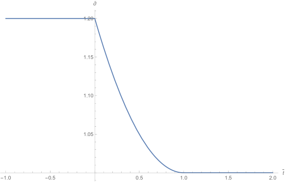
Figure 1: The profile width evolution.

The axial density profile $h(z,t)$ is depicted for $\bar{t}=0$ and $\bar{t}=1$ in figure 2, and for any time in between in figure 3

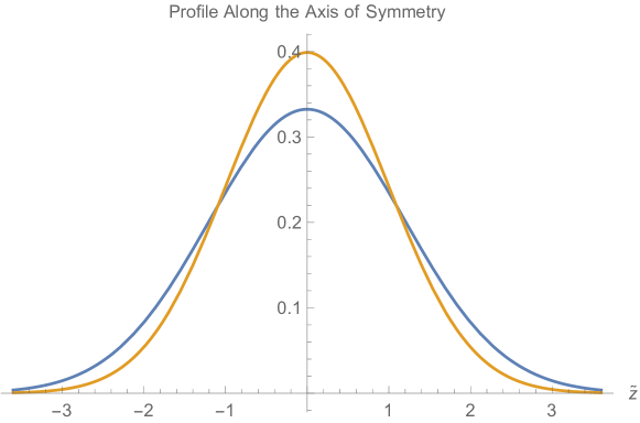
Figure 2: Axial density profile for $\bar{t}=0$ and $\bar{t}=1$.

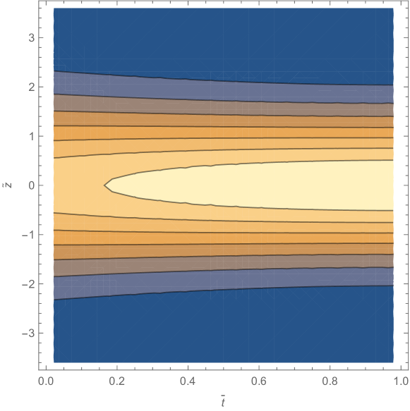
Figure 3: Axial density profile between $\bar{t}=0$ and $\bar{t}=1$.

We note that for the current profile the mass $M$ is constant although the density profile is time dependent, we also note that for the current density profile we have $\Lambda=1$ according to equation (23).

We are now in a position to calculate $\psi_{N}$ and $\psi_{r}$ using equation (46), equation (47) and equation (51). We shall choose a point of distance $r$ from the origin along the $x$ axis located at the $z=0$ plane to evaluate $\psi$, since the density profile is cylindrically symmetric every point in the $z=0$ plane of distance $r$ to the origin is equivalent to any other. Taking into account equation (42) we have:

$$\psi_{N}(\tilde{r},\bar{t})=\int\frac{\tilde{r}}{\tilde{R}}h(\tilde{z}^{\prime},\bar{t})d\tilde{z}^{\prime},\qquad\tilde{R}=\sqrt{\tilde{z}^{\prime 2}+\tilde{r}^{2}}.$$ (53)

The function $\psi_{N}(\tilde{r},0.5)$ is depicted in figure 4 in which it is clear that $\psi_{N}$ asymptotically approaches $1$.

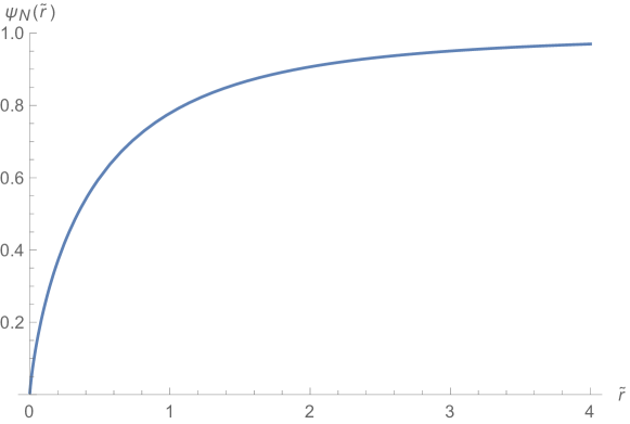
Figure 4: The function $\psi_{N}(\tilde{r},0.5)$, it is clear that $\psi_{N}$ approaches $1$ asymptotically.

Taking into account equation (41) we have:

$$\psi_{r}(\tilde{r},\bar{t})=\int\frac{\tilde{r}}{\tilde{R}}h(\tilde{z}^{\prime},\bar{t}-\frac{R}{ct_{f}})d\tilde{z}^{\prime}.$$ (54)

Hence we have another length scale $R_{s2}=ct_{f}$ which is conveniently chosen to be $R_{s2}=2R_{s}$. The function $\psi_{r}(\tilde{r},0.5)$ is depicted in figure 5 in which it is clear that $\psi_{r}$ also asymptotically approaches $1$.

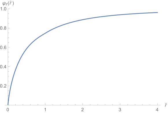
Figure 5: The function $\psi_{r}(\tilde{r},0.5)$, it is clear that $\psi_{r}$ approaches $1$ asymptotically.

The difference between the two functions $\Delta\psi$ is defined in equation (44) and depicted in figure 6. It is clear that the difference exist and does not depend on a Taylor expansion, it also clear that this difference may be approximated by a simple function to about $\tilde{r}=1$, or starting at $\tilde{r}=1$ and using a simple function to describe the function outwards which would work for at least $\tilde{r}=4$. To see that the function $\Delta\psi$ indeed approached $0$ asymptotically as predicted by equation (44) the $\tilde{r}$ axis is extended to $\tilde{r}=20$ as depicted in figure 7.

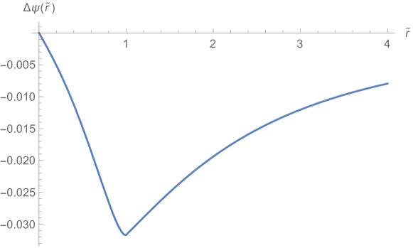
Figure 6: The function $\Delta\psi(\tilde{r},0.5)$ depicted up to $\tilde{r}=4$.

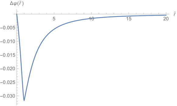
Figure 7: The function $\Delta\psi(\tilde{r},0.5)$ depicted up to $\tilde{r}=20$.

To conclude this section we shall discuss the applicability of a Taylor expansion of the type used in equation (15). In the current context, we study the function $h(\tilde{z},\bar{t})$, that is we would like to know how good is the approximation:

$$\Delta h(\tilde{z},\bar{t},\Delta\bar{t})\equiv h(\tilde{z},\bar{t}+\Delta\bar{t})-h(\tilde{z},\bar{t})\simeq\Delta h_{a}(\tilde{z},\bar{t},\Delta\bar{t}),\qquad\Delta h_{a}(\tilde{z},\bar{t},\Delta\bar{t})\equiv\Delta\bar{t}h^{(1)}(\tilde{z},\bar{t})+\frac{1}{2}\Delta\bar{t}^{2}h^{(2)}(\tilde{z},\bar{t})$$ (55)

The numerical evaluation of the functions $\Delta h(\tilde{z},\bar{t},\Delta\bar{t})$ and $\Delta h_{a}(\tilde{z},\bar{t},\Delta\bar{t})$ are depicted in figure 8 for the plane $z=0$ and for the time $\bar{t}=0.5$. It is easy to see that the approximation is indeed a good one for $|\Delta\bar{t}|<0.5$, otherwise the approximation is not valid especially for a negative $\Delta\bar{t}$ which is our main concern in retardation theory.

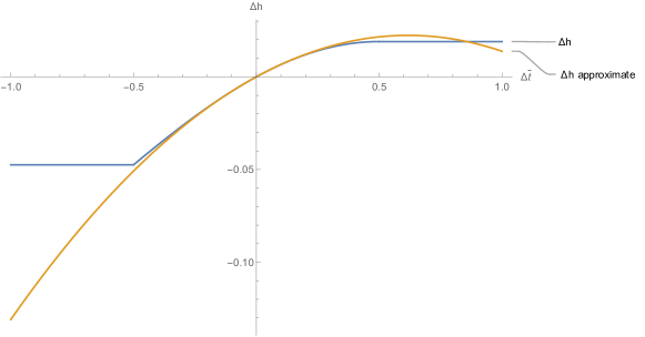
Figure 8: The functions $\Delta h(0,0.5,\Delta\bar{t})$ and $\Delta h_{a}(0,0.5,\Delta\bar{t})$.

The next step is to set the retardation delay $\Delta\bar{t}=-\frac{R}{ct_{f}}=-\frac{R}{R_{s2}}=-\frac{\tilde{R}}{\tilde{R}_{s2}}$ and calculate the approximate form of $\Delta\psi$:

$$\Delta\psi(r,\bar{t})=\psi_{r}(r,\bar{t})-\psi_{N}(r,\bar{t})=\int\frac{\tilde{r}}{\tilde{R}}\Delta h(\tilde{z}^{\prime},\bar{t},-\frac{\tilde{R}}{\tilde{R}_{s2}})d\tilde{z}^{\prime}\simeq\Delta\psi_{a}(r,\bar{t}).$$ (56)

We may try the following approximation:

$$\Delta\psi_{aw}(r,\bar{t})\equiv\int_{-\infty}^{\infty}\frac{\tilde{r}}{\tilde{R}}\Delta h_{a}(\tilde{z}^{\prime},\bar{t},-\frac{\tilde{R}}{\tilde{R}_{s2}})d\tilde{z}^{\prime}=-\frac{\tilde{r}}{\tilde{R}_{s2}}\int_{-\infty}^{\infty}h^{(1)}(\tilde{z}^{\prime},\bar{t})d\tilde{z}^{\prime}+\frac{\tilde{r}}{2\tilde{R}_{s2}}\int_{-\infty}^{\infty}\frac{\tilde{R}}{\tilde{R}_{s2}}h^{(2)}(\tilde{z}^{\prime},\bar{t})d\tilde{z}^{\prime}.$$ (57)

However, notice that for many points in the integration domain $|\frac{\tilde{R}}{\tilde{R}_{s2}}|$ is not smaller than $\frac{1}{2}$ hence $\Delta h_{a}$ is not a valid approximation. Moreover, notice that:

$$\int_{-\infty}^{\infty}h^{(1)}(\tilde{z}^{\prime},\bar{t})d\tilde{z}^{\prime}=\frac{\partial}{\partial\bar{t}}\int_{-\infty}^{\infty}h(\tilde{z}^{\prime},\bar{t})d\tilde{z}^{\prime}=\frac{\partial}{\partial\bar{t}}1=0.$$ (58)

Hence:

$$\Delta\psi_{aw}(\tilde{r},\bar{t})=\frac{\tilde{r}}{2\tilde{R}_{s2}}\int_{-\infty}^{\infty}\frac{\tilde{R}}{\tilde{R}_{s2}}h^{(2)}(\tilde{z}^{\prime},\bar{t})d\tilde{z}^{\prime}.$$ (59)

However, $\Delta\psi_{aw}(r,\bar{t})$ does not have the asymptotic property $\lim_{r->\infty}\Delta\psi_{aw}(r,\bar{t})=0$ described in equation (44) as can be seen by a numerical evaluation presented in figure 9. We conclude that $\Delta\psi_{aw}$ is not an adequate approximation of $\Delta\psi$.

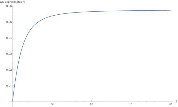
Figure 9: The asymptotic behaviour of $\Delta\psi_{aw}(\tilde{r},\bar{t})$ is clearly not appropriate.

Notice, however, that this problem can be somewhat elevated if one integrates close enough to the galactic plane $z=0$ such that $|\frac{\tilde{R}}{\tilde{R}_{s2}}|<0.5$ and consider small $\tilde{r}$. Indeed, most of the mass in centered close to the galactic plane. After some numerical experimentation we obtained a reasonable approximation integrating in the range: $[-0.25\tilde{\sigma}_{i},0.25\tilde{\sigma}_{i}]$:

$$\Delta\psi_{ac}(r,\bar{t}) \equiv \int_{-0.25\tilde{\sigma}_{i}}^{0.25\tilde{\sigma}_{i}}\frac{\tilde{r}}{\tilde{R}}\Delta h_{a}(\tilde{z}^{\prime},\bar{t},-\frac{\tilde{R}}{\tilde{R}_{s2}})d\tilde{z}^{\prime}$$ (60)

$$= -\frac{\tilde{r}}{\tilde{R}_{s2}}\int_{-0.25\tilde{\sigma}_{i}}^{0.25\tilde{\sigma}_{i}}h^{(1)}(\tilde{z}^{\prime},\bar{t})d\tilde{z}^{\prime}+\frac{\tilde{r}}{2\tilde{R}_{s2}}\int_{-0.25\tilde{\sigma}_{i}}^{0.25\tilde{\sigma}_{i}}\frac{\tilde{R}}{\tilde{R}_{s2}}h^{(2)}(\tilde{z}^{\prime},\bar{t})d\tilde{z}^{\prime}.$$

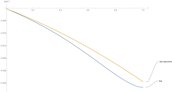
Figure 10: $\Delta\psi(\tilde{r},0.5)$ and $\Delta\psi_{ac}(\tilde{r},0.5)$ for $\tilde{r}<1$.

As a final comment we stress again that $R_{s}$ is the scale of the "galactic sphere of influence" that is the typical dimension of the region with which the galaxy exchanges mass and not necessarily the galactic radius. Thus the domain $\tilde{r}<1$ may stretch far beyond the galaxy itself.

7 Conclusions

The phenomena of retardation is ubiquitous in physics, and follows directly from the Lorentz symmetry group. Hence, any system that is invariant under the Lorentz transformation will exhibit retardation phenomena. Those include physical systems related to classical electromagnetism  Tuval ; YahalomT ; Yahalom3 ; Yahalom4 General Relativity YaRe1 ; ge ; YaRe2 ; YahalomSym , but also to other Lorentz invariant theories such as conformal gravity Mannheim0 ; Mannheim1 ; Mannheim2 .

Dark matter being a major candidate to explain galactic rotation curves has only a slim chance to being found, given that accelerator experiments, as using the Large Hadron Collider was unable to find any super symmetric particles, not only of the community’s favorite form of dark matter, but also the form of it that is mandated in string theory, a theory that also suggests a quantized version of Einstein gravity.

We have shown that at least on the galactic scale dark matter is not needed YaRe1 ; ge ; YaRe2 ; YahalomSym ; Wagman , as the dynamics can be explained by a retarded gravitational potential when a near field approximation is used. We remark that the analysis of far field leading to gravitational waves Einstein2 was corroborated in recent years by observations Taylor ; Castelvecchi .

A justification for the second order Taylor series approximation which we used in previous works is given here for the first time, showing that indeed higher order terms can be safely neglected.

We also show that one may discuss retardation phenomena without relying on a Taylor expansion.

This paper has a single author, which has done all the reported work.

This research received no funding.

MDPI stays neutral with regard to jurisdictional claims in published maps and institutional affiliations.