Comparing the spatial and kinematic distribution of gas and young stars around the shell-like structure in the CMa OB1 association

Abstract

Context. The relationship between young stellar clusters and respective parental molecular clouds is still an open issue: for instance, are the similarities between substructures of clouds and clusters just a coincidence? Or would they be the indication of a physical relationship? In order to address these issues, we have studied the CMa OB1/R1 region that shows evidence for a complex star formation history.

Aims. We obtained molecular clouds mapping with the IRAM-30 metre telescope to reveal the physical conditions of an unexplored side of the CMa region aiming to compare the morphology of the clouds with the distribution of the young stellar objects (YSOs). We also study the clouds kinematics searching for gradients and jet signatures that could trace different star formation scenarios.

Methods. The YSOs were selected on the basis of astrometric data from Gaia EDR3 that characterise the moving groups. The distance of 1099${}_{-24}^{+25}$ pc was obtained for the sample, based on the mean error-weighted parallax. Optical and near-infrared photometry is used to verify the evolutionary status and circumstellar characteristics of the YSOs.

Results. Among the selected candidates we found 40 members associated with the cloud: 1 Class I, 11 Class II, and 28 Class III objects. Comparing the spatial distribution of the stellar population with the cores revealed by the ¹³CO map, we verify that peaks of emission coincide with the position of YSOs confirming the association of these objects to their dense natal gas.

Conclusions. Our observations support the large-scale scenario of the CMa shell-like structure formed as a relic of successive supernova events.

1 Introduction

OB associations are ideal sites to test our understanding of star formation and how this process is influenced by the feedback from massive stars. The interplay between supernova (SN) events and the star-forming molecular cloud is of key relevance to the star formation process as shown by several examples. In particular, it has been proposed that SN are able to affect star formation negatively by suppressing the formation of new stars in their surroundings, and positively by triggering it (see review by Hensler et al., 2011). In the latter case, the expansion of SN remnant (SNR) shells can sweep up the surrounding gas up to the point of triggering sequential star formation (according to the “collect and collapse” model of Elmegreen & Lada, 1977).

The extended HII region Sh 2-235, for instance, is an active star-forming region, where star formation triggered by a SNR seems to have occurred in two nebulae: S235A and S235B (Kirsanova et al., 2014). The young stars associated with both nebulae are $\sim$0.3 Myr old, coinciding with the age of the SNR proposed by Kang et al. (2012). Another interesting example is W28 SNR (Lefloch et al., 2008; Vaupré et al., 2014), whose interaction with molecular clouds could have triggered the formation of nearby protostellar clusters in the Trifid nebula. In the case of the SNR IC443, however, although many young stellar objects (YSOs) are found surrounding the SNR shell, the SNR proved to be too young as compared to the age of YSOs and could not have triggered their formation (Xu et al., 2011). The recent numerical simulations by Dale et al. (2015) could easily reproduce triggering of star formation. However, when comparing with observations the authors show that triggered star formation is much harder to infer, since they could not discriminate triggered from non-triggered objects.

Star formation is, in any case, often found nearby SNRs, for instance there are several SNRs associated with YSOs in the Large Magellanic Cloud (e.g. Desai et al., 2010), and supernovae have been long suggested to be exciting the star formation in their surroundings. The arc-shaped Sh 2-296 nebula is one of these cases, which is suspected to be an old SNR that could have triggered the formation of new stars in CMa OB1 (Herbst & Assousa, 1977).

The Canis Major OB1/R1 (henceforth CMa, for simplicity) is a nearby (d $\sim$ 1 kpc) OB Association with a complex star formation history. Our previous studies showed that the region contains young objects originated from different star-forming events (Gregorio-Hetem et al., 2009; Santos-Silva et al., 2018).

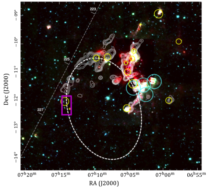
Figure 1: Overview of the CMa R1 region. The background is a RGB composite WISE image (Red: 22.2 $\mu$m, Green: 12.1 $\mu$m, Blue: 3.4 $\mu$m). A dashed straight line gives longitudes in the Galactic Plane, and the dashed ellipse shows the area of the CMa shell suggested by Fernandes et al. (2019). White contours trace the molecular gas (¹³CO). X-ray observations with XMM-Newton (Santos-Silva et al., 2018) are indicated by cyan circles, and the groups of YSOs studied by Fischer et al. (2016) are shown by yellow circles. The area studied here is marked by the magenta box. (Figure adapted from Fernandes et al., 2019).

A promising hypothesis is presented by Fernandes et al. (2019) showing new evidence that Sh 2-296, the most prominent nebula in the CMa Association, is part of a large (diameter $\sim$ 60 pc) shell-like structure. Figure 1 shows this structure, called the CMa shell, that likely results from successive SN explosions from 6 to 1 Myr ago as inferred from the past trajectories of three runaway stars in the region, derived from Gaia proper motions. They also found evidence that the CMa shell is related to a larger ($\sim$ 140 pc in size) shell structure, visible in H$\alpha$. However, the older population of low-mass stars (¿ 10 Myr), which are confirmed CMa members, cannot be explained by these recent SN explosions suggesting that they may be causally related to the existence of the H$\alpha$ super-shell.

Fernandes et al. (2019) suggest that the present-day configuration of the star-forming gas may have been shaped by a few successive SN explosions that occurred several Myr in the past. Despite the evidence of SN events shaping the CMa shell, Fernandes et al. (2019) argue that they probably played a minor role in triggering star formation in these clouds.

CMa is, therefore, an ideal laboratory for probing how the feedback from SNRs interacting with molecular clouds can affect their environment and subsequent star formation and evolution in OB associations.

2 Molecular clouds in CMa

A ¹³CO (J = 1-0) survey of Kim et al. (2004), using the Nagoya-4m telescope with a beam width of 2.^′7, identified 13 molecular clouds in the area of the CMa Association, distributed in three main structures around the clouds No. 3 (l$\sim$224^o, b$\sim-$2^o), No. 4 (l$\sim$224.^o5, b $\sim-$1^o), and No. 12 (l $\sim$226^o, b$\sim-$0.^o5).

Partial maps of these molecular clouds were recently obtained with the 1.85m mm-submm Telescope installed at the Nobeyama Radio Observatory. According to Onishi et al. (2013), the 1.85m telescope is dedicated to a large-scale survey aiming to reveal the physical properties of molecular clouds in the Milky Way Galaxy. In the 1.3mm band, observations of the rotational transition $J$= 2–1 of ¹²CO, ¹³CO and C¹⁸O were obtained with a beam size of 2.^′7.

The ¹³CO map shows a chain of molecular clouds that extends North-East of the Sh 2-296 nebula. In Fig. 2a, the main structure associated with Sh 2-296 is called “West cloud”, which coincides with “Cloud 3” of the list from Kim et al. (2004). This is the largest cloud of the region with mass $\sim$ 16000 M_⊙ and an area of 358 pc². To the North-East, the second main structure, called “East cloud”, is related to “Cloud 4” (total mass $\sim$ 12000 M_⊙, and area $\sim$ 301 pc²).

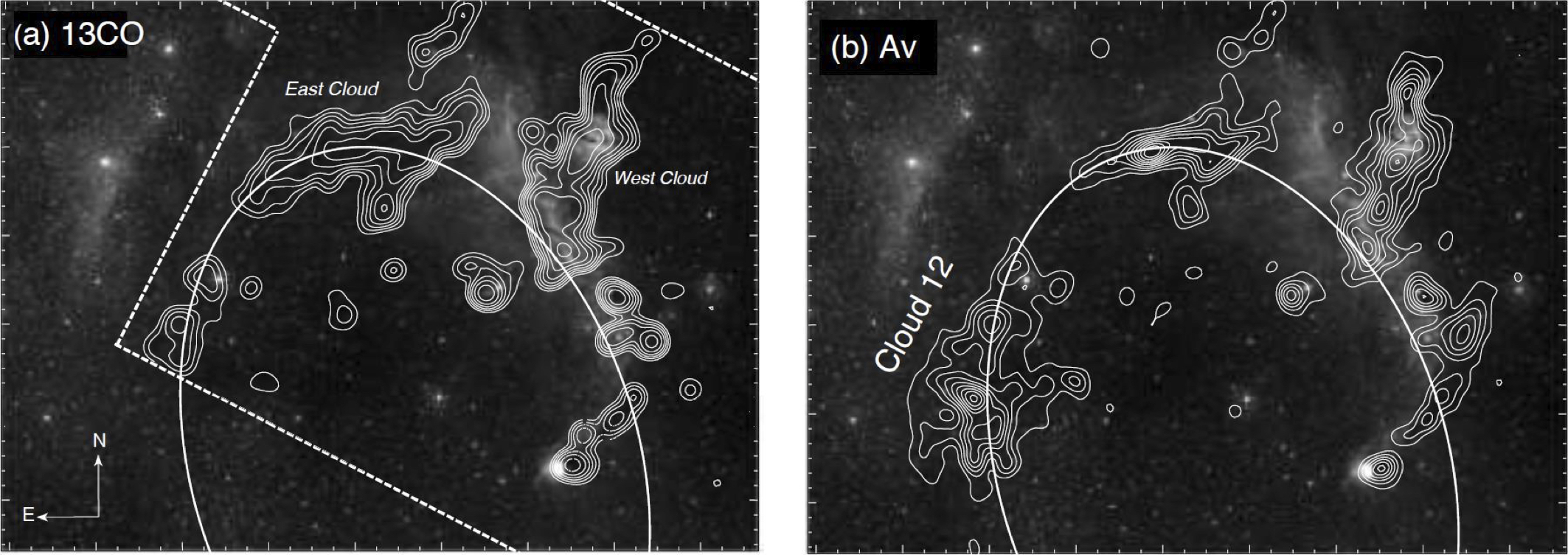
Figure 2: DSS2-Red image of the Sh 2-296 nebula. The ellipse marks the proposed shape of the CMa shell and the contours in each panel trace: (a) the ¹³CO emission (courtesy of the Osaka group, see Onishi et al. (2013)); (b) extinction ($A_{V}$) from the 2MASS maps of Dobashi et al. (2011). (Figure adapted from Fernandes et al., 2019).

The clouds are also traced by the dust distribution revealed by the extinction map of A_V (Fig. 2b) from Dobashi et al. (2011). We can see that the dust emission matches closely the ¹³CO distribution, following the approximate shape of the CMa shell. Comparing Figs. 2a and 2b, it can be noted the lack of information about ¹³CO emission for “Cloud 12”, which is found in the area not covered in the survey obtained by the Osaka group (see the dashed rectangle in Fig. 2a). This cloud is the third largest gas reservoir in the CMa association, with an estimated mass of 7500 M_⊙ and an area of 315 pc² (Kim et al., 2004). Besides its important amount of gas, this cloud is located in the border of the CMa Shell, in the opposite side of Sh 2-296 nebula.

This work is dedicated to investigate this complementary area of gas distribution, which can bring an important contribution to understand the star formation scenario in CMa. In the general context, we aim to explore the global dynamics that allows us to search for signatures of the large-scale SNR driven shock and its interaction with the molecular gas condensation. In Sect. 3, we summarise the surveys used in the analysis and the molecular gas observations. The identification and analysis of young stars associated with the cloud are presented in Sect. 4. Finally, in Sect. 5 we discuss the results from the molecular clouds mapping in comparison with the characteristics of the associated stellar population. The conclusions are summarized in Sect. 6.

3 Observational data

3.1 Dust continuum surveys

Besides the visual extinction map that was compared with the molecular clouds distribution in Sect. 2, we analyze here the dust distribution traced by the infrared emission. We are particularly interested in searching for condensations and filamentary structures aiming to verify whether they are harbouring pre- and protostellar cores, as suggested by Elia et al. (2013).

As part of the Herschel Infrared Galactic plane survey (Hi-GAL Molinari et al., 2010), Elia et al. (2013) conducted a study of star formation in the third Galactic quadrant, which includes the CMa region. In such study, Herschel PACS and SPIRE photometric observations were combined with NANTEN CO $J$=1–0 observations of cores and clumps, revealing that most of the protostars are in the early accretion phase, while star formation is still underway in cores distributed along filaments.

The filamentary structure of “Cloud 12” studied here can be clearly seen in the Herschel SPIRE map obtained at 250 $\mu$m, which is shown in Fig. 3 (left panel). The position of bright infrared sources (flux density $>$ 3 Jy at 100 $\mu$m band) from the IRAS Catalogue of Point Sources (Helou & Walker, 1988) is also plotted in this figure, showing a good correlation with the bright filaments.

We also performed the characterisation of the IR sources associated with the clouds by searching for candidates in the AllWISE catalogue (Cutri et al., 2013). The WISE photometry (Wright et al., 2010) at bands W1 (3.4 $\mu$m), W2 (4.6 $\mu$m), and W3 (12 $\mu$m) are useful to distinguish different classes of YSOs as a function of their IR excess.

As shown in Fig. 1, the CMa clouds contain several groups of YSO candidates identified by Fischer et al. (2016) based on WISE colors. The candidates were selected by adopting the criteria proposed by Koenig & Leisawitz (2014) to identify Class I and Class II objects. Details on this method, which is also applied by us, is presented in Sect. 4.2.1. The distribution of the groups of YSOs found by Fischer et al. (2016) closely follows the border of the CMa Shell and coincides with the gas distribution.

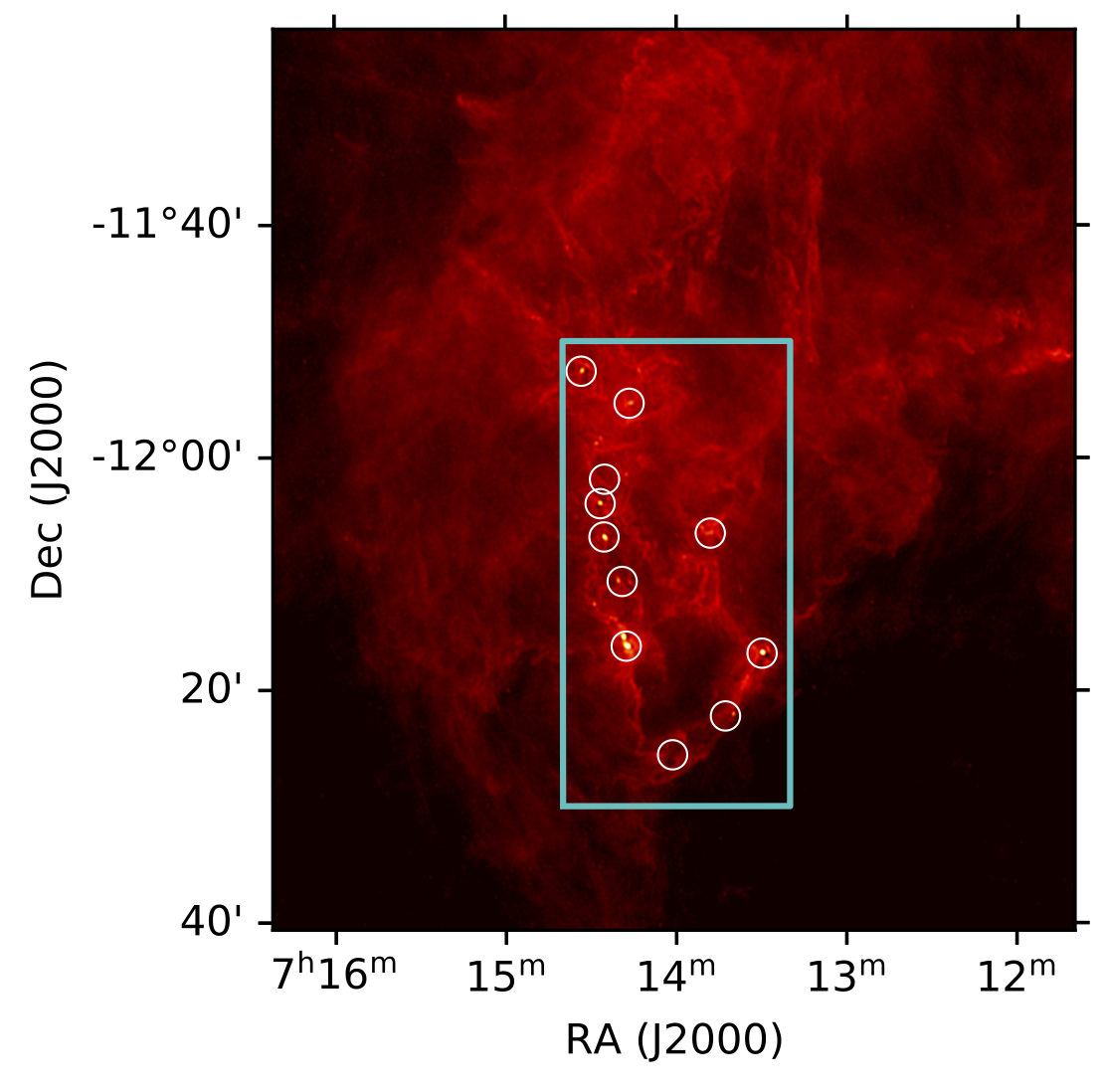
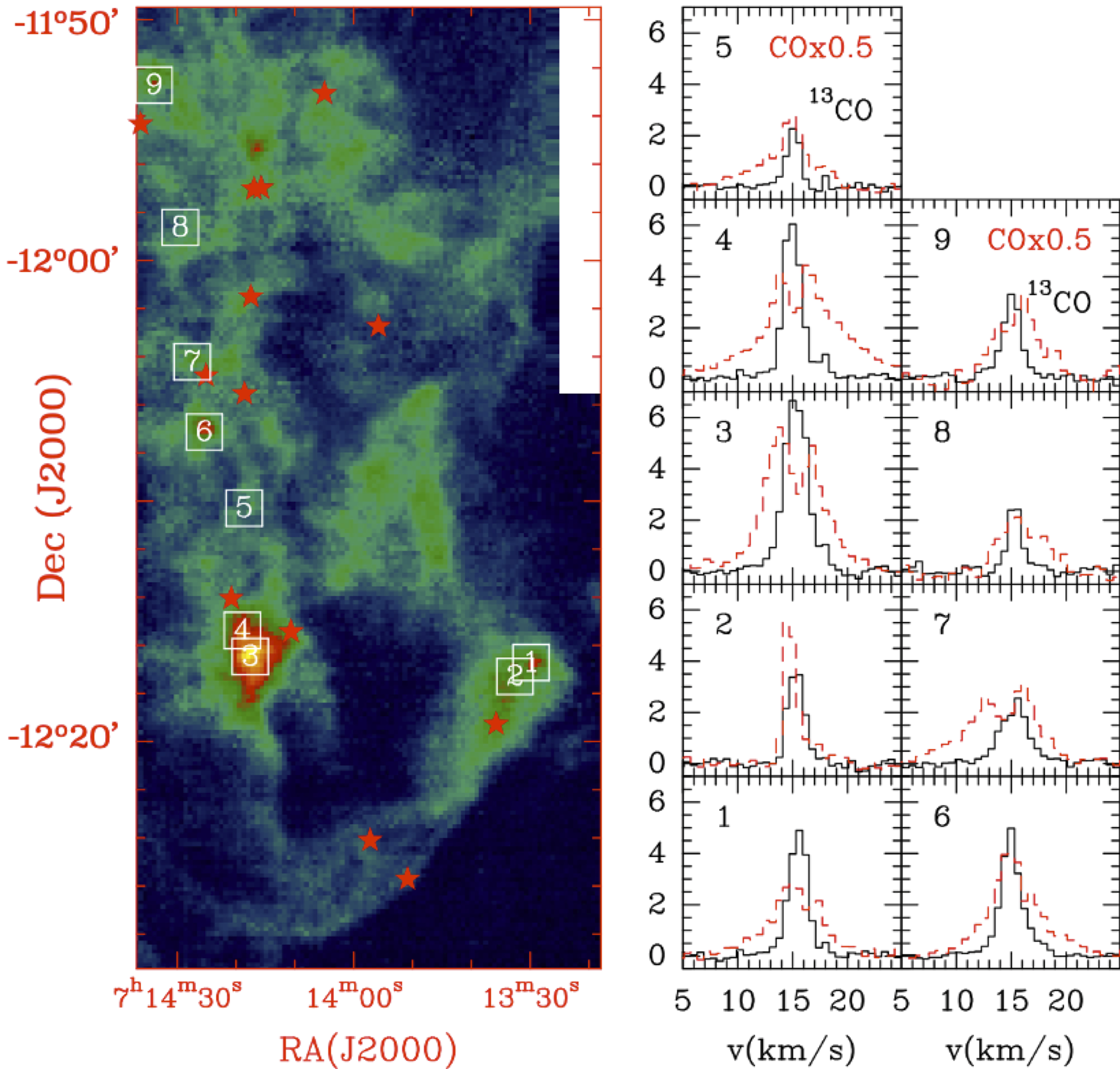
Figure 3: Left: The region covered by the IRAM observations (cyan box) overlaid on the Herschel SPIRE 250$\mu$m map that illustrates the filamentary structure of the cloud and the distribution of bright IRAS sources (white circles). Middle: ¹³CO map revealing dense cores roughly related to the IRAS sources. The location of the WISE sources (Class I) are marked by red stars. The location of the 9 dense cores listed in Table 1 is drawn with white squares. Right: The core emission ($T_{MB}$) observed in the ¹³CO (black) and ¹²CO (dashed red) $J$=1–0 transitions. A scaling factor of 0.5 has been applied to the ¹²CO line intensity.

Table 1: Observational properties of a sample of molecular cores.

Core	$\Delta\alpha$	$\Delta\delta$	RA (J2000)	Dec (J2000)	Tkin	N(13CO)	N(H2)	outflow	comment
	(arcsec)	(arcsec)	( h m s )	( ∘  ′  ′′ )	(K)	($10^{16}$cm-2)	($10^{22}$cm-2)
1	$-$325	165	07 13 30	$-$12 16 43	8	3.3	2.1	Y
2	$-$285	130	07 13 33	$-$12 17 18	8	3.3	2.1	N
3	375	180	07 14 17	$-$12 16 28	13	5.0	3.3	Y	Broad wings
4	395	245	07 14 18	$-$12 15 23	13	3.5	2.3	Y	Broad wings
5	390	550	07 14 18	$-$12 10 18	10	3.8	2.5	Y	Broad wings
6	490	740	07 14 25	$-$12 07 08	12	1.2	0.8	Y	Small wings
7	520	915	07 14 27	$-$12 04 13	12	0.7	0.5	Y	Blueshifted wing
8	550	1250	07 14 29	$-$11 58 38	7	0.7	0.5	N
9	615	1605	07 14 33	$-$11 52 43	9.5	1.2	0.8	N

Note: The physical parameters: kinetic temperature (T_kin), and column density (N(¹³CO)) were obtained from averaging the signal over a region of $20^{\prime\prime}\times 20^{\prime\prime}$. A value T_kin = 10K was adopted for Core 5 due to the lack of detection of C¹⁸O.

3.2 Molecular gas

In order to characterise the properties of the cores and filaments associated with the star formation activity, as revealed in the AllWISE and Herschel surveys, we have used the IRAM-30m telescope (Sierra Nevada, Spain) to map the emission of the ground state rotational transition $J$=1–0 of CO and its rare ¹³CO and C¹⁸O isotopologues in Cloud 12. Observations were carried out during three observing runs in October 2018 (project 043-18), March 2019 (project 120-19) and October 2019 (project 034-20), using the EMIR receiver at 3mm in its 2SB mode connected to the FTS spectrometer in its 192 kHz resolution mode. Observations were carried out using the “On-The-Fly” mode. We chose a reference position, which we checked to be free of emission in the CO $J$=1–0 line. We mapped a total area of 20^′ $\times$ 40^′ in the rotational transitions $J$=1–0 of CO, ¹³CO and C¹⁸O. Figure 3 (left panel) shows the mapped area superimposed upon an image of the continuum emission from Cloud 12 obtained by Herschel SPIRE at 250 $\mu$m (see Sect. 3.1).

The weather conditions were good and rather stable during the observing sessions. Atmospheric calibrations were performed every 12 to 15 min and showed the weather to be stable. Pointing was monitored every hour on a nearby quasar and corrections were always found lower than 3^′′. Special attention was paid to the line calibration and we obtained a very good agreement between the different runs. The calibration uncertainty is about 10% in the 3mm band.

The data reduction was performed using the GILDAS software developed at IRAM. The line intensities are expressed in units of antenna temperature corrected for atmospheric attenuation and rearward losses ($T_{A}^{*}$). For the subsequent radiative transfer analysis of the pre- and protostellar core emission, line fluxes were expressed in units of main beam temperature ($T_{MB}$). The main beam efficiency and the half power beam width (HPBW) were taken from the IRAM webpage.

The right panel of Fig. 3 illustrates the pre- and protostellar condensations, that were detected thanks to the IRAM-30m angular resolution. Table 1 gives the results for a sample of molecular cores shown in Fig. 3 (middle panel).

4 Stellar population

Two groups of YSOs (Fischer et al., 2016) are projected unto the eastern border of the CMa shell, coinciding with the location of the “Cloud 12” identified by Kim et al. (2004). Our preliminary analysis on the distribution of YSO candidates (selected from the AllWISE catalogue) is well correlated with the dust distribution revealed by the A_V map in a 800 arcmin² area within the cloud (Fig. 2).

Here, we extracted optical and infrared data (public catalogues) for stars found in the direction of the fields observed with IRAM-30m, searching for candidates that probably are members associated to the cloud (Sect. 4.1). The selected members are then characterized, based on infrared colors that allow us to identify Classes I and II objects (Sect. 4.2.1). The confirmation of the pre-main sequence nature of the candidates is obtained from color-magnitude diagram using Gaia EDR3 photometry (Sect. 4.2.2).

4.1 Selection of members

Aiming to exclude the presence of field-stars in the sample, as well as confirming the membership of the objects associated with the cloud, we performed a selection of kinematic members by using the techniques described by Hetem & Gregorio-Hetem (2019). Following the formalism presented by Dias et al. (2014), the adopted statistical methods use likelihood model and cross entropy technique to estimate the probability of a candidate to be (or not to be) considered a cluster member. A vector of parameters consisting of astrometric and kinematic data given by the observed proper motion is used to calculate the probability density function for a candidate and for the background of field-stars. The membership probability basically results from the fitting of a Gaussian in 5D phase space (three positions and two components of proper motion) by comparison with the Gaussian background. Since the cross entropy is sensitive to the initial parameters, a genetic algorithm code is adopted for parameters optimisation (Hetem & Gregorio-Hetem, 2019).

The first subset of candidates was obtained by querying astrometric and kinematic data from the Gaia EDR3 catalogue (Gaia Collaboration, 2016b, 2020a). The search was performed in an area slightly larger than the fields observed with IRAM-30m. We also delimited the query in ranges of parallax and proper motion compatible with results previously found for CMa (e.g. Santos-Silva et al., 2021). According to the Gaia technical recommendations, we applied the RUWE $<1.4$ and $\varpi/\sigma_{\varpi}>3$ selection filters, in order to avoid low quality of the astrometric solution.

Table 2 gives the intervals of parameters adopted for the catalogue query, as well as the results found for our sample. The mean values obtained for proper motion define the membership criteria. An illustration of the reliability of the method is given in Fig. 4 (left panel), were the distribution of probabilities is presented as a function of modulus of proper motion $|\mu|$ = $[(\mu_{\alpha})^{2}+(\mu_{\delta})^{2}]^{0.5}$. We suggest that objects with membership probability P $\geq$ 50% are very likely associated with the ambient cloud, which are considered here very-likely CMa members. These members have ($\mu_{\alpha}$, $\mu_{\delta}$) within 1$\sigma$ of the mean values found for the sample. Objects appearing below the dashed line (P$<$50%) in Fig. 4 (left panel) are considered candidates or probable field-stars, since they have proper motion parameters in ranges that are larger than the 1$\sigma$ threshold adopted by us.

Table 2: Limits used for the Gaia data query and results from the kinematic members selection.

ID	RA	Dec	$\varpi$	$\mu_{\alpha}$	$\mu_{\delta}$
	(J2000)	(J2000)	(mas)	(mas/yr)	(mas/yr)
query range	07h13m to 07h15m	$-$12∘35′ to $-$11o45′	0.4 to 2	$-$7 to 1	$-$4 to 4
P$\geq$50%	07h13$.\!\!^{\rm m}$7 to 07h14$.\!\!^{\rm m}$4	$-$12∘14′ to $-$11o58′	0.87 $\pm$ 0.30	$-$3.26 $\pm$ 0.44	1.08 $\pm$ 0.46
CMa06	07h03$.\!\!^{\rm m}$7 to 07h05$.\!\!^{\rm m}$6	$-$11∘34′ to $-$11o00′	0.85 $\pm$ 0.09	$-$4.18 $\pm$ 0.36	1.52 $\pm$ 0.21
Sh 2-296	07h01$.\!\!^{\rm m}$2 to 07h06$.\!\!^{\rm m}$8	$-$12∘12′ to $-$10o48′	0.8 to 1.25	$-$4.10 $\pm$ 0.60	1.50 $\pm$ 0.40

Note: Our sample (P$\geq$50%) is compared with clusters CMa06 (Santos-Silva et al., 2021) and Sh 2-296 (Gregorio-Hetem et al., 2021) located to the W direction of the CMa shell.

Santos-Silva et al. (2021) use HDBScan technique to fit 5 parameters from Gaia aiming to explore the stellar clusters and sub-groups in the entire CMa region. No sub-group was found by them in the area studied here, probably due to the low number of members, and/or the objects are too faint to be identified by the automatic procedure. However, it is interesting to compare our results with those found by Santos-Silva et al. (2021) for the group they called as CMa06, which coincides with the Sh 2-296 nebula (see West cloud in Fig. 2a). Despite the fact that this cluster is located on the opposite side of the CMa shell ( $\sim$ 2^o to the W), its parallax and proper motion are quite similar to the results of our sample. This may be due to a common star formation history. A similar result was independently achieved by Gregorio-Hetem et al. (2021) in the study of objects associated to Sh 2-296 using the same method adopted here (Hetem & Gregorio-Hetem, 2019), which validates our criteria to select the cloud members. The results found for CMa06 and Sh 2-296 are also presented in Table 2.

In order to evaluate the error-weighted parallax, we adopted the calculation used by Navarete et al. (2019), based on the uncertainty on measured parallax ($\varpi$) and the spatial correlation between the position of the sources. We obtained for our sample the mean parallax $\langle\leavevmode\nobreak\ \pi\leavevmode\nobreak\ \rangle$= 0.91$\pm$0.02 mas that was converted to the distance of 1099${}_{-24}^{+25}$ pc. Figure 4 (right panel) shows the distribution of parallaxes and error bars given in Table 3, highlighting 11 stars (2 Class II and 9 Class III) that coincide with the secondary structure of the cloud found in the centre of the gas distribution, discussed in Sect. 5.

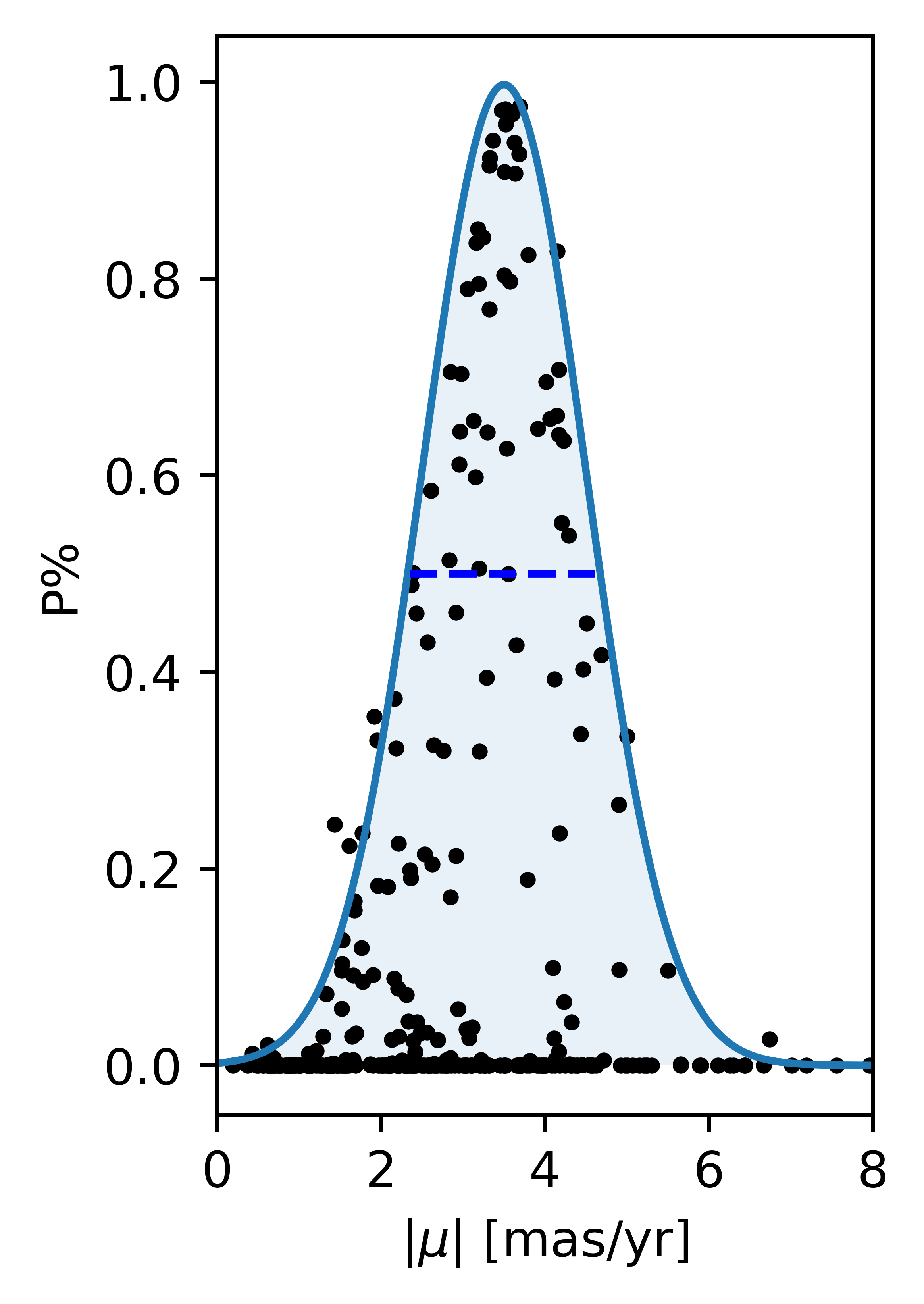
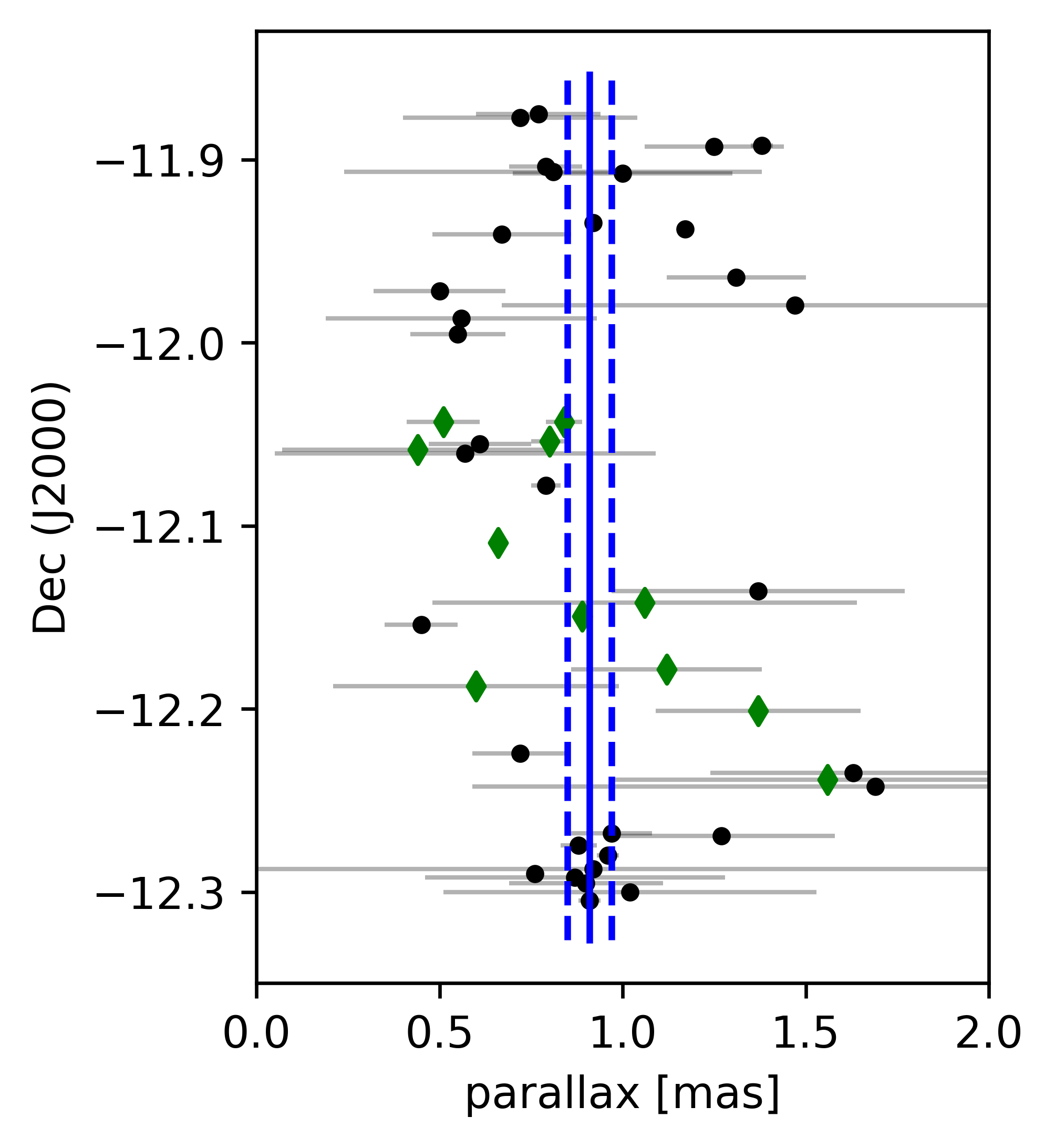
Figure 4: Left: Distribution of membership probabilities as a function of modulus of proper motion. A dashed line is used to separate members from candidates. Right: Parallax distribution for the sample showing the observed values of $\varpi$ and respective error bars. Green $\blacklozenge$ symbols indicate the sources found in the secondary structure of the cloud (see Sect. 5). The vertical blue lines indicate the error-weighted mean parallax $\langle\leavevmode\nobreak\ \pi\leavevmode\nobreak\ \rangle$=0.91$\pm$0.02 mas (dashed lines show 3$\sigma$ deviation).

4.2 Characterisation

4.2.1 Infrared excess

The infrared (IR) data from AllWISE catalogue were used for two purposes: (i) characterizing the stars that were selected as members of CMa, on the basis of proper motion, and (ii) searching for embedded sources that were not detected by Gaia probably due to high levels of extinction in dense regions. The query was restricted to the same area described in Sect. 4.1.

Our analysis of IR-excess is based on colour-colour diagrams using WISE bands: W1 (3.4 $\mu$m), W2 (4.6 $\mu$m) and W3 (12 $\mu$m) that are useful to distinguish different classes of pre-main sequence stars. Based on the results from Rebull et al. (2014) for the Taurus star-forming region, Koenig & Leisawitz (2014) proposed the limits on the [W1$-$W2] $\times$ [W2$-$W3] diagram defining the expected locus for Class I and Class II objects, due to their significant IR-excess compared with Class III objects and field-stars.

In order to ensure the photometric quality, we extracted from the AllWISE catalogue only the sources in agreement with the following conditions for the magnitude measured at 12 $\mu$m: $0.45<W3_{r\chi^{2}}<1.15$ and $W3_{snr}>5$, where $r\chi^{2}$ and $snr$ correspond to the photometric error and signal-to-noise ratio, respectively. According to Koenig & Leisawitz (2014) these filters are applied with the purpose of mitigating contamination from fake detections.

Figure 5 displays the [W1$-$W2] $\times$ [W2$-$W3] diagram for 383 sources that coincide with the fields observed with IRAM-30m and that are common on both catalogues: Gaia and WISE, which membership probability is represented by different symbols. It can be noted that most of the studied objects (89%) are plotted in the region where Class III and/or field-stars are expected to be found.

Our final sample contains 40 members (1 is Class I; 11 are Class II; and 28 are Class III) confirmed by proper motion (P$\geq$ 50%), and 4 candidates (1 is Class I, and 3 are Class II). Since we are mainly interested in embedded objects, Class III candidates (P$<$50%) were not included in the sample. Table 3 gives the list of objects and the Gaia EDR3 parameters used in the membership probability calculation. The division between the classes of objects is indicated by double-lines in Table 3.

Aiming to complement the list of objects, we also searched for WISE sources not detected by Gaia. Due to the lack of membership information for these additional sources, we consider here as possible members only Class I or Class II objects. In other words, among the WISE candidates not detected by Gaia, the Class III objects were not taken into account due to the difficult in distinguishing them from field-stars. By this way, the sample is complemented by 45 WISE sources that we consider possible members (12 are Class I, and 33 are Class II). The distribution of the sources in the equatorial coordinates space is shown in Fig. 6 (left panel). The infrared photometry used in the analysis of the stellar population is given in Table 4 for the same list presented in Table 3.

We have verified in our sample the presence of H$\alpha$ emitters by using a cross-correlation with the results from Pettersson & Reipurth (2014) that revealed 353 new H$\alpha$ stars in the direction of CMa. The area surveyed by us contains 10 H$\alpha$ stars. However, only 4 of them coincide with the CMa members, meaning that the other H$\alpha$ stars have proper motion and/or parallax in disagreement with the kinematic selection criteria adopted by us. In Table 3 we add a comment identifying each of the H$\alpha$ stars identified by Pettersson & Reipurth (2014), which are classified by us as Class II objects. For classical T Tauri stars, the H$\alpha$ emission is an evidence of accretion process that is expected for Class II objects and is also related to the presence of a circumstellar disk. The characteristics of these 4 H$\alpha$ stars are in agreement with their young age ($<$ 5 Myr), which is estimated in the next section.

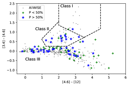
Figure 5: WISE colour-colour diagram displaying the expected locus for Class I and Class II sources as proposed by Koenig & Leisawitz (2014). Confirmed members (blue $\star$) have P $\geq$ 50%, while possible members (green $+$) have P $<$ 50%. The remaining AllWISE objects (grey dots) are not present in Gaia EDR3 catalogue. IR sources found in the Classes I and II boxes are considered here as additional candidates.

4.2.2 Cluster Age

In order to confirm the youth of the sample we constructed the color-magnitude diagram using the photometric data at bands $G$ ($\sim$ 600 nm), G_BP ($\sim$ 500 nm), and G_RP ($\sim$ 700 nm) from Gaia EDR3. The magnitudes were corrected for reddening by adopting the A_λ/A_V relations from Cardelli et al. (1989). For each source, we calculate the distance modulus given by its parallax, which was used to estimate the unreddened absolute magnitude $(M_{G})_{0}$.

Figure 6 (right panel) shows the distribution of our sample in the $(M_{G})_{0}\times[G_{BP}$-$G_{RP}]_{0}$ diagram compared with isochrones from PARSEC (Bressan et al., 2012; Marigo et al., 2017). The models for 1 Myr and 5 Myr were adopted to indicate the range of ages previously reported for the CMa young population (Gregorio-Hetem et al., 2009), while the 100 Myr isochrone was chosen as representative of the ZAMS (Zero Age Main Sequence).

In the color-magnitude diagram we display only the sources with good photometric data, which show snr $>$ 10 in all bands. Some of the Class III objects show a good fit with the ZAMS indicating that we adopted a suitable mean value of visual extinction (A_V = 0.9 mag) in the reddening correction. Since the Class III objects are not affected by circumstellar IR-excess, we argue that this low level of A_V corresponds to the interstellar reddening in the direction of CMa, which is in agreement with the extinction map of the region (Gregorio-Hetem, 2008). We conclude that it is highly probable that the Class III stars are observed in the near vicinity, but are preferentially located in the foreground, of the cloud.

The same can be said for other sources detected by Gaia, since they are visible. However, some of them are too faint ($(M_{G})_{0}>$ 8 mag in right panel of Fig. 6), probably due to a reddening that needs be corrected with a higher value of A_V, which should be evaluated individually. This can be the case of sources that are still surrounded by some amount of cloud material.

We are aware that using optical color-magnitude diagram gives only a rough estimation of age. Despite of that, it can be noted that most of the sources exhibiting IR excess (Class I and Class II) are $\sim$ 5 Myr or younger. Several of the Class III presented here are in the same range of age and a few sources seem to be older, but still are in the pre-main sequence phase, confirming the youth of our sample. Among the Gaia EDR3 sources, we do not find massive stars. The brightest Class III objects have colors similar to 2 M_⊙ stars.

As mentioned in Sect. 4.1 the proper motion of our sample, which is located in the E side of the CMa shell, coincides with the values found for group CMa06 located to the W. The estimated age for this group is 6$\pm$1 Myr (Santos-Silva et al., 2021), suggesting that these two stellar clusters, which are located at opposite sides, may have had a similar star formation scenario.

5 Comparing gas and star distributions

As can be seen in Figs. 3 and 6 the projected spatial distribution of our sample of stars closely follows the filamentary structure present in the ¹³CO gas. Most of the Class II sources are found around dense cores, probably emerged from the cloud and still associated with it.

In Fig. 7 we plot a mosaic of ¹³CO maps showing in each panel a different range of gas velocity, from 12.6 km/s to 19.2 km/s. A main structure with V = 15 $\pm$ 1.2 km/s is clearly seen at RA$\sim$ 07^h14$.\!\!^{\rm m}$5, growing from N to S and then continuing to SW. A secondary structure at V = 17.4 $\pm$ 1.2 km/s appears then at the centre of the plot (RA = 07^h14^m, Dec = 12^∘10^′). Despite their partial overlapping, they seem to be two structures representing different parts and/or movements of the cloud. The relative motions of these two gas structures are suggestive of a large-scale expanding gas motions around the cavity detected in the molecular gas at IRAM and in the continuum emission with SPIRE (see Fig. 3). It is remarkable that the “cavity” looks void of young stars and protostars.

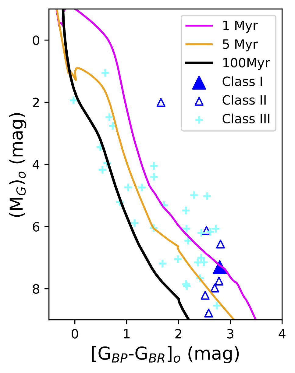
Figure 6: Left: Equatorial coordinates of Class I (filled symbols) and Class II (open symbols) that are CMa members (triangles) and additional candidates from AllWISE catalogue (circles). Right: Absolute magnitude as a function of colour from Gaia data for the CMa members (P $\geq$ 50%). The magnitudes are corrected for extinction. We use isochrones from PARSEC models, by adopting the 100 Myr line as representative of the ZAMS.

The presence of these two cloud structures and their connection with the stellar population is confirmed by analyzing the gas kinematics through moment maps similar to the works by Álvarez-Gutiérrez et al. (2021) and Stutz & Gould (2016), for instance. Based on the ¹³CO observations, we obtained the Moment 1 (mean velocities) map that is presented in Fig. 8 overlaid by the distribution of the YSOs that are Class I and Class II objects (the same presented in Fig. 6). For Gaia sources we also display the proper motion vectors, in order to compare the velocity dispersion of stars with the radial velocity of the gas. The map clearly shows the secondary structure with velocities V $>$ 17 km/s, while the gas in the main structure of the cloud has velocities ranging from less than 15 km/s to $\sim$ 16.5 km/s, which supports the discussion based on Fig. 7. For our sample of YSOs, the proper motion velocity dispersion, measured in the plane of the sky, shows no remarkable trend that could indicate non-isotropic velocity patterns. This prevents us to address here a deeper integration of the stellar content with the gas kinematics for cloud sub-structures.

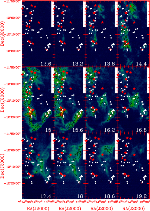
Figure 7: Molecular gas mapping (¹³CO) as a function of velocity given in km/s (see right bottom of each panel). The position of WISE sources is shown for Class I (red stars) and Class II (white squares) objects.

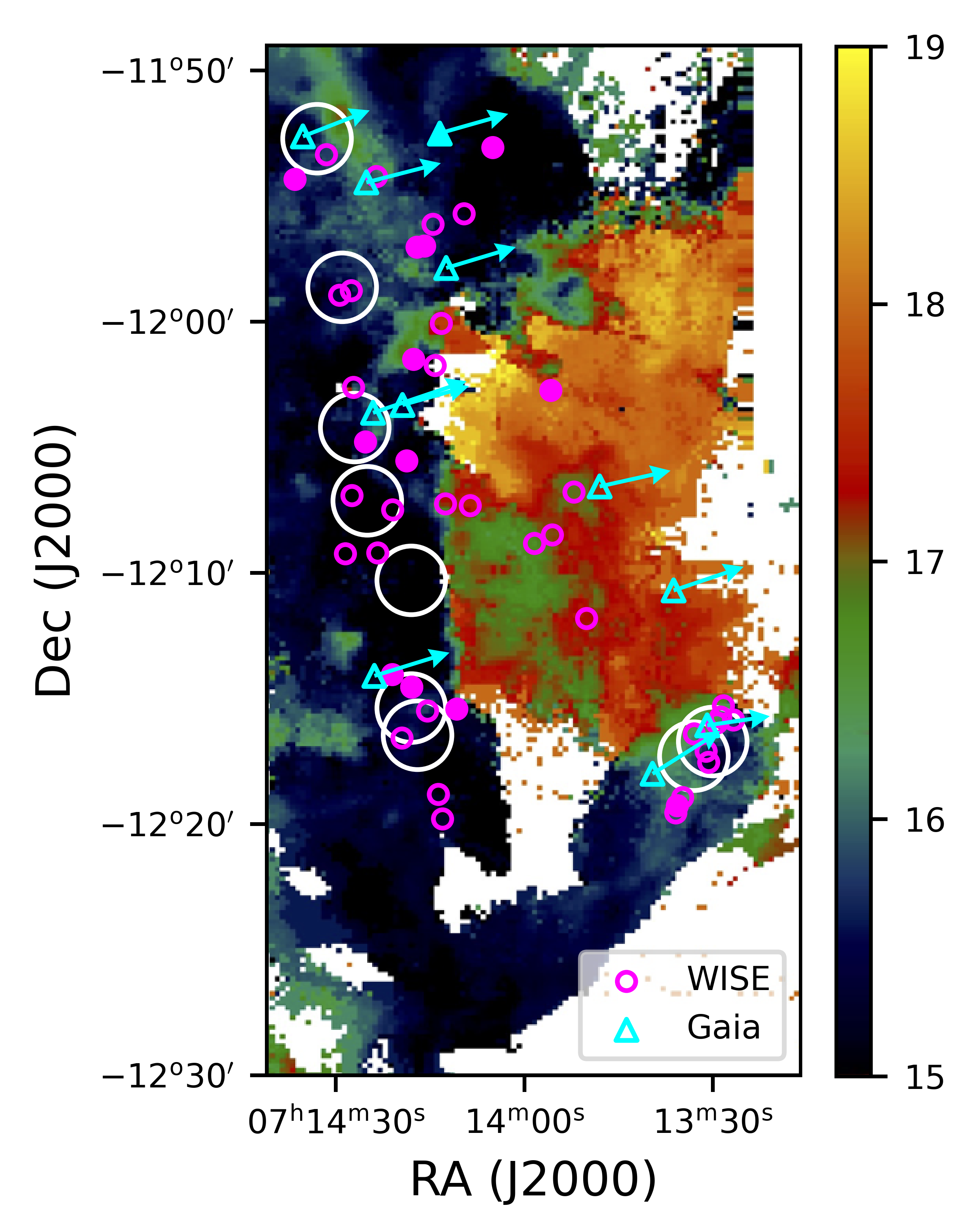
Figure 8: Moment 1 map showing the distribution of velocities measured in km/s, based on ¹³CO data. The proper motion vectors are displayed for the YSOs that are Gaia sources (same symbols as Fig. 6). White circles indicate the position of dense cores (see Fig. 3).

Mapping of the molecular line emission reveals the presence of dense cores, detected in the lines of ¹³CO and CS. A sample of 9 cores was investigated in more detail. The ¹²CO and ¹³CO line profiles are displayed in the right panel of Fig. 3. The observed line profiles were fitted by using a simple modeling of the¹³CO and C¹⁸O lines, adopting a canonical relative abundance ratio [¹³CO]/[C¹⁸O] = 8. This allowed us to estimate the optical depths $\tau_{13}$ and $\tau_{18}$ of both isotopologues. The observed line profiles and optical depths were subsequently modelled with the radiative transfer code MADEX (Cernicharo, 2012) in the Large-Velocity Gradient approximation (Sobolev, 1958, 1960) using the CO-H₂ collisional coefficients of Yang et al. (2010) and the line-width (FWHM) measured from a gaussian fit to the line profiles. We could check that the results are essentially independent of n(H₂) in the regime of densities 10⁴ $-$ 10⁶ cm^-3, typical of dark clouds and star-forming cores, i.e the ground state transitions are thermalized.

MADEX was adopted by us to derive the kinetic temperature and the molecular gas column density in the cores. The main result is that these cores consist of cold gas, with temperatures in the range 8–13 K. One of the most direct signs of protostellar activity is the signature of mass-loss phenomena (outflows) as broad wings in the CO rotational line profiles observed towards dense cores. This is illustrated in the CO lines profiles of cores 1, 3, 4, 5, 6 and 7 in Fig. 3. In the case of core 4, the outflow wings reach velocities as high as 20 km/s that is clear evidence for active, possibly massive, star formation in the core. Some of these cores, like e.g. cores 6 and 7, are associated with IR (WISE) sources, and we note that many of the IR sources coincide with the ¹³CO cores identified in our map. We speculate that the absence of IR sources in the other cores which display bipolar outflow signatures indicates that the driving protostars might be at earlier stage of evolution, possibly Class 0.

Conversely, other dense cores detected in our observations appear to be in a quiescent stage, as illustrated by cores 2, 8 and 9 (Fig. 3). Based on our molecular gas content analysis presented in Table 1, it appears that the cores in the Northern part of the region ($n\geq 6$) tend to have lower gas column densities. More work is needed to confirm this trend (higher densities found in the Southern part of the cloud), based on a very reduced sample, and to investigate whether it is related to the physical or chemical (depletion ?) evolution of the region.

Despite all the dense cores (kinetic temperatures from 10 to 14 K) are found in the main structure, with most of the stellar members associated to it, there are 1 Class I and 8 Class II sources located in the direction of the secondary, smaller cloud structure. Since only two of these stars are Gaia sources, we cannot evaluate kinematic differences compared with the stars associated with the main structure.

Indeed, no trend is observed when comparing the spatial distribution of sources having proper motion vectors displayed in Fig. 8. The same can be said for the parallax distribution (see Fig. 4), where 9 Class III sources are also highlighted because they appear in the secondary structure, but without showing trends on $\varpi$. However, it is interesting to note that 2MASS07134800-1206336, found in the secondary structure, is the brightest star of the Class II objects (G_Gaia = 13 mag), which appears in the red side of the color-magnitude diagram (see Fig. 6, right panel), with age $<$ 1 Myr. The parallax of this bright source indicates it is in the largest distance ($\varpi$ = 0.62 $\pm$ 0.04) compared with the other members. Therefore, it is possible that the reddening still needs to be corrected for this source and its mass shall be larger than 2 M_⊙.

Table 3: Membership probability, parallax, proper motion and Gaia EDR3 photometry.

Gaia EDR3	P	$\varpi$	$\mu_{\alpha}$	$\mu_{\delta}$	G	GBP	GRP
	%	mas	mas/yr	mas/yr	mag	mag	mag
3045239083971370112	87	$0.77\pm 0.17$	$-3.21\pm 0.16$	$0.91\pm 0.15$	$18.65$	$20.43$	$17.24$
3045208886056506112	13	$1.69\pm 1.10$	$-2.52\pm 0.86$	$0.97\pm 1.06$	$20.33$	$21.63$	$18.78$
3045225516172964864a	95	$0.66\pm 0.02$	$-3.32\pm 0.02$	$0.74\pm 0.02$	$13.80$	$14.77$	$12.74$
3045229291445342592b	92	$1.31\pm 0.19$	$-3.26\pm 0.18$	$0.98\pm 0.16$	$18.80$	$20.42$	$17.43$
3045227749555916032c	91	$0.61\pm 0.14$	$-3.11\pm 0.16$	$0.88\pm 0.13$	$17.93$	$19.59$	$16.63$
3045131301773079168	90	$0.79\pm 0.10$	$-3.02\pm 0.08$	$1.04\pm 0.09$	$17.44$	$19.06$	$16.22$
3045208950479742208	83	$1.12\pm 0.26$	$-3.28\pm 0.20$	$1.11\pm 0.18$	$18.89$	$20.72$	$17.57$
3045237434703416320	82	$1.63\pm 0.39$	$-3.52\pm 0.34$	$1.09\pm 0.33$	$19.89$	$21.26$	$18.52$
3045235785435946624	79	$0.72\pm 0.32$	$-3.13\pm 0.26$	$1.22\pm 0.24$	$19.03$	$20.96$	$17.65$
3045117141257872000	78	$1.00\pm 0.30$	$-3.49\pm 0.28$	$0.90\pm 0.29$	$19.01$	$20.52$	$17.75$
3045215998525392384d	65	$0.97\pm 0.11$	$-2.93\pm 0.11$	$0.43\pm 0.10$	$17.29$	$19.13$	$15.91$
3045116114758900736	65	$0.57\pm 0.52$	$-4.38\pm 0.53$	$1.48\pm 0.54$	$19.99$	$21.22$	$18.57$
3045114804796665984	63	$1.02\pm 0.51$	$-3.17\pm 0.44$	$2.00\pm 0.48$	$19.85$	$21.54$	$18.39$
3045214070080777600	27	$0.92\pm 1.18$	$-2.78\pm 0.90$	$0.44\pm 1.00$	$20.66$	$21.37$	$19.22$
3045234170527254656	21	$0.45\pm 0.10$	$-3.00\pm 0.10$	$0.87\pm 0.09$	$17.39$	$19.19$	$16.07$
3045235785436006400	21	$1.47\pm 0.80$	$-3.48\pm 0.62$	$0.54\pm 0.63$	$20.26$	$21.51$	$18.81$
3045118416872687744	92	$0.96\pm 0.03$	$-3.69\pm 0.03$	$0.99\pm 0.03$	$12.85$	$12.97$	$12.63$
3045226821842999552	97	$0.80\pm 0.05$	$-3.51\pm 0.06$	$1.03\pm 0.06$	$16.32$	$17.39$	$15.29$
3045213352825581312	97	$0.89\pm 0.02$	$-3.28\pm 0.02$	$0.99\pm 0.02$	$14.03$	$14.49$	$13.40$
3045228368031224448	96	$0.84\pm 0.05$	$-3.23\pm 0.05$	$1.15\pm 0.05$	$15.86$	$16.64$	$14.99$
3045215758007221632	94	$0.79\pm 0.04$	$-3.19\pm 0.04$	$0.94\pm 0.04$	$15.85$	$16.76$	$14.87$
3045232555619709056	93	$1.17\pm 0.02$	$-3.60\pm 0.02$	$0.83\pm 0.02$	$14.50$	$14.87$	$13.97$
3045114809098665984	92	$0.76\pm 0.02$	$-3.22\pm 0.01$	$1.01\pm 0.01$	$12.60$	$12.99$	$12.02$
3045229291444432384	90	$0.50\pm 0.18$	$-4.08\pm 0.16$	$1.06\pm 0.14$	$18.59$	$20.14$	$17.32$
3045114701716408832	90	$0.90\pm 0.21$	$-3.53\pm 0.18$	$1.11\pm 0.20$	$18.70$	$20.30$	$17.46$
3045114843459884288	90	$0.87\pm 0.41$	$-3.71\pm 0.33$	$1.46\pm 0.36$	$19.60$	$20.97$	$18.36$
3045209156636885760	85	$0.72\pm 0.13$	$-2.71\pm 0.11$	$0.94\pm 0.09$	$17.68$	$19.11$	$16.52$
3045114396781820672	84	$0.91\pm 0.03$	$-3.11\pm 0.02$	$0.96\pm 0.02$	$14.53$	$14.88$	$14.02$
3045118382511875712	82	$0.88\pm 0.05$	$-3.90\pm 0.04$	$0.97\pm 0.04$	$15.81$	$16.43$	$15.05$
3045227509039371648	80	$0.44\pm 0.37$	$-2.95\pm 0.36$	$0.94\pm 0.30$	$19.39$	$20.99$	$18.11$
3045233242814458752	79	$0.67\pm 0.19$	$-2.92\pm 0.20$	$1.19\pm 0.22$	$18.63$	$20.13$	$17.47$
3045229879859736704	70	$0.51\pm 0.10$	$-4.33\pm 0.09$	$1.11\pm 0.10$	$17.53$	$18.91$	$16.38$
3045207885326442496	70	$1.27\pm 0.31$	$-3.06\pm 0.24$	$0.87\pm 0.23$	$19.34$	$20.71$	$18.19$
3045228952146750208	70	$0.55\pm 0.13$	$-2.88\pm 0.14$	$1.02\pm 0.12$	$18.11$	$20.01$	$16.81$
3045130678995758848	69	$1.37\pm 0.28$	$-3.63\pm 0.33$	$1.67\pm 0.34$	$19.26$	$20.84$	$17.97$
3045130472837058176	66	$1.56\pm 0.59$	$-2.26\pm 0.70$	$0.83\pm 0.72$	$20.20$	$21.74$	$18.88$
3045420954362862336	64	$1.38\pm 0.03$	$-3.52\pm 0.03$	$1.56\pm 0.03$	$15.32$	$15.85$	$14.62$
3045212936208209024	64	$0.60\pm 0.39$	$-2.34\pm 0.30$	$1.02\pm 0.33$	$19.33$	$20.77$	$18.11$
3045233693790633472	62	$1.25\pm 0.19$	$-2.80\pm 0.17$	$1.70\pm 0.16$	$18.58$	$19.99$	$17.43$
3045233281473783936	59	$0.92\pm 0.01$	$-3.01\pm 0.02$	$1.00\pm 0.02$	$13.50$	$13.92$	$12.89$
3045213623404184448	58	$1.37\pm 0.40$	$-2.63\pm 0.36$	$0.66\pm 0.31$	$19.46$	$21.21$	$18.14$
3045233998728534272	56	$0.56\pm 0.37$	$-2.45\pm 0.29$	$1.47\pm 0.27$	$19.58$	$20.97$	$18.31$
3045233487625692160	53	$0.81\pm 0.57$	$-3.79\pm 0.78$	$1.65\pm 0.95$	$20.07$	$21.24$	$18.75$
3045225202636012800	50	$1.06\pm 0.58$	$-3.88\pm 0.61$	$0.45\pm 0.64$	$20.04$	$21.43$	$18.73$

Notes: The objects are separated by: Class I (top); Class II (middle); Class III (bottom), according with Table 4. Stars identified as H$\alpha$ emitters are indicated by (a) ID 381; (b) ID 387; (c) ID 390; and (d) ID 392, where the ID numbers are given by Pettersson & Reipurth (2014).

6 Conclusions

We mapped molecular clouds with the IRAM-30m to investigate the properties of cores and filaments in order to determine the spatial and kinematic distributions of gas in the cloud and their relation with the star formation activity. In the general context, we aim to search for and characterise the shock driven by the SN into the molecular cloud, which would be responsible for the gas compression and gravitational collapse.

Comparing the spatial distribution of the stellar population with the cores revealed by the ¹³CO map, we verify that peaks of emission coincide with the position of YSOs (see Fig. 3). These results confirm that CMa harbors pre- and protostellar cores showing that star formation is still underway in cores distributed along filaments, as suggested by Elia et al. (2013) based on a survey with Herschel.

We selected a sample of 89 sources, 40 of them are confirmed members (Gaia EDR3) associated to CMa. The mean error-weighted parallax was converted to the distance of 1099${}_{-24}^{+25}$ pc, which is in excellent agreement with previous results for the CMa region (Clariá, 1974; Tovmasyan et al., 1993; Shevchenko et al., 1999). Using the WISE colors, the sources were characterized according with the IR-excess. We are mainly interested here on Classes I and II that may have circumstellar disk. All of these disk-bearing stars are found around the filamentary structure of the cloud, despite several of them are not embedded, but probably located in the cloud foreground. The color-magnitude diagram constructed with the G_Gaia photometry were used to verify whether the selected sources truly are pre-main sequence stars. The ages are less than 5 Myr for most of the sources, coinciding with ages estimated for the cluster found in the opposite side of the CMa shell. Moreover, as shown in Fig. 5 (right panel) and discussed below, the presence of embedded objects corresponding to protostellar phase (Class 0 and Class I sources) is confirmed in our sample. Since Class 0 and Class I stars have typical ages of 10⁴ to 10⁵ yr, they can be considered a direct evidence for sequential star formation in the region.

The kinematic analysis reveals the presence of two structures representing different parts of the cloud. A main structure, exhibiting V = 15 $\pm$ 1.2 km/s, is formed from N to S in an extended stripe where most of the dense cores are found and YSOs are associated with. The secondary structure, seen at V = 17.4 $\pm$ 1.2 km/s, grows from the SW to the centre of Fig. 3 (middle panel). Evidence of outflows is remarkable from the broad wings in the CO rotational line profiles observed in 6 dense cores, which are suggested to be sites of protostellar activity as indicated by their association with IR sources, and shows that a burst of star formation is currently going on. Follow up observations, such as near-IR spectroscopy to obtain radial velocity of the members, are required to confirm the trends of stellar members following the cloud structure observed for this limited sample of objects associated to the studied region.

Despite these are partial results, they shed some light attempting to explain the star formation in CMa. The age of the Class II population is consistent with the age/timescale of the SNRs (Fernandes et al., 2019). The similarity of the young stellar population properties on East/Western sides of the shell supports the scenario of a large-scale gravitational collapse of the shell, most likely induced by the SN explosions.

We tentatively suggest that the presence of young protostellar population (with massive and/or intermediate-mass objects, as indicated by the strong outflow emission) could indicate that a second episode of star formation has recently taken place. The distribution of YSOs in the two gas layers at 15 and 17 km/s suggests that local events on the Eastern side (the region surveyed at IRAM) have contributed to drive the current star formation process. Our observations of the region altogether support the large-scale scenario of SNR shock-driven, but other processes at smaller scales appear to have influenced and possibly induced the local star formation.

Table 4: Infrared photometry for stellar population.

Gaia EDR3	2MASS	J	H	K	W1	W2	W3	W4	Class
		mag	mag	mag	mag	mag	mag	mag
3045239083971370112	07141347-1152298	14.44	12.88	11.82	10.97	9.82	6.99	4.61	I
3045208886056506112	07141796-1214324	15.55	14.05	13.13	11.60	10.46	7.88	5.63	I
3045225516172964864	07134800-1206336	10.79	9.62	8.65	7.62	7.00	4.55	2.66	II
3045229291445342592	07141244-1157517	15.24	13.89	12.94	11.40	10.61	8.49	6.41	II
3045227749555916032	07141939-1203191	13.39	12.11	11.29	10.32	9.66	7.51	5.74	II
3045131301773079168	07133622-1210420	14.09	12.89	12.24	12.04	11.40	8.67	6.45	II
3045208950479742208	07142387-1214061	15.06	13.94	13.45	12.66	11.91	8.71	5.69	II
3045237434703416320	07143525-1152374	15.79	14.37	13.56	12.79	12.13	10.54	5.78	II
3045235785435946624	07142515-1154273	15.02	13.74	12.92	11.77	11.20	9.96	8.38	II
3045117141257872000	07133088-1216043	15.21	14.02	13.45	12.73	11.98	9.56	7.42	II
3045215998525392384	07142409-1203377	13.20	11.99	11.32	10.40	9.57	7.20	4.77	II
3045116114758900736	07133958-1217599	15.54	14.04	13.27	12.56	12.03	9.86	7.85	II
3045114804796665984	07140707-1217153	15.73	14.87	14.32	13.98	13.48	10.03	7.68	II
3045214070080777600	07142847-1209146	15.65	14.24	13.20	12.39	11.49	9.07	6.47	II
3045234170527254656	07142755-1158460	13.72	12.58	12.07	11.39	10.69	8.47	6.48	II
3045235785436006400	07142353-1154135	15.57	14.19	13.32	12.39	11.71	9.72	7.41	II
3045118416872687744	07133684-1216484	12.36	12.30	12.23	12.20	12.22	12.39	9.09	III
3045226821842999552	07135758-1203138	13.71	12.96	12.79	12.76	12.68	12.27	9.14	III
3045213352825581312	07140300-1208579	12.61	12.20	12.07	12.04	12.05	11.67	8.50	III
3045228368031224448	07135653-1202357	13.74	13.14	12.92	12.84	12.88	12.41	9.07	III
3045215758007221632	07143221-1204404	13.33	12.83	12.50	12.47	12.39	12.00	8.71	III
3045232555619709056	07140255-1156164	13.36	13.02	12.93	12.95	12.98	11.62	8.90	III
3045114809098665984	07141006-1217243	11.28	11.12	11.00	10.87	10.87	9.43	7.40	III
3045229291444432384	07141365-1158183	15.07	14.21	13.78	13.53	13.47	12.37	9.00	III
3045114701716408832	07141366-1217431	15.13	14.28	13.94	13.62	13.63	10.67	8.42	III
3045114843459884288	07140167-1217317	16.24	15.64	15.33	15.60	15.44	12.60	9.21	III
3045209156636885760	07143327-1213273	14.53	13.68	13.34	13.10	13.05	12.12	9.17	III
3045114396781820672	07140309-1218168	13.47	13.14	13.07	13.03	13.08	11.97	8.84	III
3045118382511875712	07134177-1216279	14.08	13.51	13.40	13.28	13.31	12.52	8.74	III
3045227509039371648	07140828-1203310	15.77	14.66	14.25	14.07	13.98	12.34	8.96	III
3045233242814458752	07134763-1156272	15.44	14.65	14.34	14.28	14.44	11.83	9.05	III
3045229879859736704	07132666-1202354	14.46	13.69	13.38	13.20	13.19	11.89	8.18	III
3045207885326442496	07142893-1216095	16.30	15.84	15.17	15.37	16.12	12.35	9.05	III
3045228952146750208	07141111-1159429	14.36	13.45	12.94	12.70	12.59	11.88	9.09	III
3045130678995758848	07133413-1212033	15.80	14.49	13.90	13.19	12.72	11.19	8.08	III
3045130472837058176	07133056-1214195	16.44	15.26	15.36	14.78	14.65	12.48	8.72	III
3045420954362862336	07133375-1153320	13.75	13.22	13.03	13.10	13.17	12.67	8.95	III
3045212936208209024	07140301-1211153	16.01	15.16	14.53	14.51	14.40	12.69	9.17	III
3045233693790633472	07135366-1153340	15.90	15.21	14.91	14.88	15.07	12.38	9.05	III
3045233281473783936	07135236-1156044	12.15	11.76	11.70	11.64	11.66	12.41	8.99	III
3045213623404184448	07141889-1208085	15.35	14.20	13.62	13.51	13.29	12.72	8.99	III
3045233998728534272	07143643-1159120	16.21	15.47	14.97	14.79	14.79	12.22	8.91	III
3045233487625692160	07135485-1154240	16.80	15.88	15.64	15.64	15.76	11.70	8.68	III
3045225202636012800	07135247-1208309	16.23	15.27	14.69	14.68	14.51	12.05	8.92	III

References

- Álvarez-Gutiérrez et al. (2021) Álvarez-Gutiérrez, R.H., Stutz, A. M., Law, C. Y., Reissl, S., Klessen, R. S., Leigh, N. W. C., Liu, H.-L., Reeves, R. A., 2021, ApJ, 908, 86
- Boch & Fernique (2014) Boch, T., Fernique, P. 2014, ASPC 485, 277B
- Bonnarel et al. (2000) Bonnarel, F. , Fernique, P. , Bienaymé, O. et al. 2000, A&AS, 143, 33B
- Bressan et al. (2012) Bressan, A., Marigo, P., Girardi, L., Salasnich, B. A. , et al. 2012, MNRAS, 427, 127B
- Cardelli et al. (1989) Cardelli, J. A., Clayton, G. C., Mathis, J. S. 1989 ApJ, 345, 245
- Cernicharo (2012) Cernicharo, J. “Laboratory astrophysics and astrochemistry in the Herschel/ALMA era”. ECLA - European Conference on Laboratory Astrophysics, Eds. C. Stehlé, C. Joblin, L. d’Hendecourt. ESA Publications Series, Vol. 58, 2012, pp.251-261
- Clariá (1974) Clariá, J.J. 1974, A&A, 37, 229
- Cutri et al. (2013) Cutri, R. M., Wright, E. L., Conrow, T., et al. 2013, The AllWISE Data Release Products
- Dale et al. (2015) Dale, J. E., Haworth, T. J., & Bressert, E. 2015, MNRAS, 450(2), 1199-1211
- Desai et al. (2010) Desai, K. M., Chu, Y.-H., Gruendl, R. A., et al., 2010, AJ, 140(2), 584-594
- Dias et al. (2014) Dias, W. S., Monteiro, H., Caetano T. C., et al. 2014, A&A, 564, 79
- Dobashi et al. (2011) Dobashi, K., 2011, PASJ, 63S, 1D
- Elia et al. (2013) Elia, D., Molinari, S., Fukui, Y., et al. 2013, ApJ, 772, 45
- Elmegreen & Lada (1977) Elmegreen, B. G., & Lada, C. J., 1977, ApJ, 214, 725
- Fernandes et al. (2019) Fernandes, B., Montmerle, T., Gregorio-Hetem, J., Santos-Silva, T., 2019, A&A, 628, 44
- Fischer et al. (2016) Fischer, W. J., Padgett, D. L., Stapelfeldt, K. L., & Sewiło, M. 2016, ApJ, 827, 96
- Gaia Collaboration (2020a) Gaia Collaboration, Brown, A. G. A., Vallenari, A., Prusti, T. et al. 2020, A&A, 595, A2
- Gaia Collaboration (2016b) Gaia Collaboration, Prusti, T., de Bruijne, J. H. J., et al. 2016, A&A, 595, A1
- Gregorio-Hetem (2008) Gregorio-Hetem J., 2008, in Reipurth B., ed., Handbook of Star Forming Regions, Vol. II, p. 1
- Gregorio-Hetem et al. (2009) Gregorio-Hetem J., Montmerle T., Rodrigues C. V., et al. 2009, A&A, 506, 711
- Gregorio-Hetem et al. (2021) Gregorio-Hetem J., Navarete, F., Hetem, A., et al. 2021, AJ 161, 133
- Griffin et al. (2010) Griffin, M. J., Abergel, A., Abreu, A. et al., 2010, A&A, 518, L3
- Helou & Walker (1988) Helou, G., Walker, D. W., 1988 Infrared astronomical satellite (IRAS) catalogues and atlases. V. 7, p.1
- Hensler et al. (2011) Hensler, G., 2011. Computational Star Formation, Proceedings of the International Astronomical Union, IAU Symposium, Volume 270, pp. 309-317
- Herbst & Assousa (1977) Herbst, W. & Assousa, G.E. 1977, ApJ, 217, 473
- Hetem & Gregorio-Hetem (2019) Hetem, A., Gregorio-Hetem, J., 2019, MNRAS 490 (2), 2521, 2541
- Kang et al. (2012) Kang, J.-h., Koo, B.-C., & Salter, C. 2012, AJ, 143, 75
- Kim et al. (2004) Kim, B. G., Kawamura, A., Yonekura, Y., & Fukui, Y., 2004. PASJ, 56(2), 313-339
- Kirsanova et al. (2014) Kirsanova, M. S., Wiebe, D. S., Sobolev,et al., 2014, MNRAS, 437, 1593
- Koenig & Leisawitz (2014) Koenig, X.P., Leisawitz, D.T., 2014, ApJ, 791, 131
- Lefloch et al. (2008) Lefloch, B., Cernicharo, J., & Pardo, J., 2008, A&A, 489, 157
- Marigo et al. (2017) Marigo, P., Girardi, L., Bressan, A., et al. 2017, ApJ, 835, 77M
- Molinari et al. (2010) Molinari, S., Swinyard, B., Bally, J., et al. 2010, PASP, 122, 314
- Navarete et al. (2019) Navarete, F., Galli, P. A. B., Damineli, A., 2019, MNRAS, 487, 2771
- Onishi et al. (2013) Onishi, T., Nishimura, A., Ota, Y., et al. 2013, PASJ, 65, 78
- Pettersson & Reipurth (2014) Pettersson, B., Reipurth, B., 2019, A&A 630, A90
- Pilbratt et al. (2010) Pilbratt, G. L., Riedinger, J. R., Passvogel, T. et al., 2010, A&A, 518, L1
- Poglitsch et al. (2010) Poglitsch, A., Waelkens, C., Geis, N., et al. 2010, A&A, 518, L2
- Rebull et al. (2014) Rebull, L. M., Padgett, D. L., McCabe, C.-E. et al. 2010, ApJS 186, 259
- Santos-Silva et al. (2018) Santos-Silva, T., Gregorio-Hetem, J., Montmerle. T. Fernandes, B., Stelzer, B., 2018, A&A, 609, 127
- Santos-Silva et al. (2021) Santos-Silva, T., Perottoni, H. D., Almeida-Fernandes, F., et al. (submitted to MNRAS)
- Shevchenko et al. (1999) Shevchenko, V. S., Ezhkova, O. V., Ibrahimov, M. A., van den Ancker, M. E., & Tjin A Djie, H. R. E. 1999, MNRAS, 310, 210
- Sobolev (1958) Sobolev, V.V., 1958 “Theorical Astrophysics”. ed. Ambartsumyan, Pergamon Press Ltd. London
- Sobolev (1960) Sobolev, V.V., 1960 “Moving Envelopes of Stars”. Harvard University Press
- Stutz & Gould (2016) Stutz, A. M., Gould, A., 2016, A&A, 590, A2
- Tovmasyan et al. (1993) Tovmasyan, H.M., Oganesyan, R. Kh., Epremyan, R.A., & Yugenen, D. 1993, AZh, 70, 451
- Vaupré et al. (2014) Vaupré, S., Hily-Blant, P., Ceccarelli, C., et al. 2014, A&A, 568, A50
- Wright et al. (2010) Wright, E. L., Eisenhardt, P. R. M., Mainzer, A. K. et al. 2010, AJ, 140, 1868
- Xu et al. (2011) Xu, J.-L., Wang, J.-J., & Miller, M., 2011, ApJ, 727(2), 81
- Yang et al. (2010) Yang et al. 2010, ApJ, 718, 1062