Tunning the tilt of a Dirac cone by atomic manipulations: application to 8Pmmn borophene
Abstract
We decipher the microscopic mechanism of the formation of tilt in the two-dimensional Dirac cone of borphene. In our ab initio calculations, we identify relevant low-energy degrees of freedom on the lattice and find that these atomic orbitals reside on an effective honeycomb lattice (inner sites), while the high-energy degrees of freedom reside on the rest of the lattice (ridge sites). Integrating out the high-energy atomic orbitals, gives rise to remarkably large effective further neighbor hoppings on the coarse grained ”honeycomb graph” of inner sites that determine the location and tilt of the Dirac cone. Molecular orbitals – that can be modified by atomic manipulations – are responsible for the creation of further neighbor edges on the honeycomb graph that controls the tilt of the resulting Dirac cone. This leads to an effective tight-binding model on a parent honeycomb graph that facilitates numerical modeling of various effects such as disorder/interactions/symmetry-breaking for tilted Dirac cone fermions. Since the tilt is a proxy to spacetime metric, our result offers a robust perspective on the fabrication of desired emergent spacetime structure and synthesis of geometric forces at ambient conditions that are likely to enhance our control on the movement of electrons in electric/optical devices.
I Introduction
The marriage between the mathematical concept of ”topology” and quantum materials lead to the birth of ”topological materials” and developments that followed afterwards. Can the (local) ”geometry” play a similar role in combination with quantum materials? In the same way that the appearance of Dirac fermions in graphene and other Dirac materials can be attributed to an emergent Minkowski spacetime structure at distances much larger than the atomic distances, quantum materials with ”tilted Dirac cone” can be naturally associated with an emergent spacetime (not merely the space) metric. In these class of materials the tilt is a proxy to spacetime geometry. We use Geometric Quantum Material (GQM) to refer to them.
Every periodic structure in quantum condensed matter is mounted on a mathematical object called lattice. Irrespective of which atoms one wishes to place on the sites of a given lattice, they come in 230 possible structures Inui et al. (1990). The presence of lattice breaks translation and rotation, and some times parity and/or time reversal invariance of the vacuum Girvin and Yang (2019). The lattice therefore breaks the Poincaré group Ryder (1996) thereby the connection between spin and statistics of the particles is lost and therefore one may have fermions with integer spin that is enforced by the irreducible representations of its space group (SG) Bradlyn et al. (2016).
Is there any other interesting consequence that can be associated with the underlying SG? To set the stage for answering this question, let us start by a simple, but profound observation Girvin and Yang (2019): Consider a simple quantum mechanical hopping process on a lattice and think about the wave equation in the continuum limit. On the square lattice the Hamiltonian becomes , while on the honeycomb lattice it becomes , namely the massless Dirac Hamiltonian Ando (2011). Therefore despite that in the continuum limit, the lattice spacing is immaterial, but still remnants of the microscopic symmetries of the pertinent SG are manifested in the long-distance behavior and decide whether the structure of the ensuing spacetime is Galilean or Minkowski. This can be regarded as an example of metamorphosis of atomic scale symmetry (SG) to a long-distance geometrical structure. The duality between atomic scale SG symmetry and long distance geometry is a central to understand the geometric structure in GQMs.
What is the microscopic mechanism of such a duality between the microscopic structure and the long-distance (low-energy) characteristics in more complicated lattice structures? The long-distance behavior of interest for us is the tilted Dirac cone band whose Hamiltonian is Tajima et al. (2006); Goerbig et al. (2008); Kajita et al. (2014); Farajollahpour2019 ; Jalali-Mola and Jafari (2019); Verma et al. (2017) where is the unit matrix. A vector-looking quantity here determines the tilt of the Dirac cone. But at a much deeper level, it can be encoded into an emergent spacetime metric Farajollahpour2019 ; Jalali-Mola and Jafari (2019); Jafari (2019); Westström and Ojanen (2017); Liang and Ojanen (2019); Volovik (2016, 2018); Nissinen and Volovik (2017), where is the Fermi velocity. Therefore the tilt of a Dirac cone is actually a proxy for an emergent solid-state spacetime structure. Since the density of states is enhanced by a , the tilted Dirac cone materials can generically give stronger responses to external stimuli 111This enhancements nicely fits into spacetime description as a ”redshift” factor Mohajerani et al. (2021).. Therefore it is crucial to understand the atomistic mechanism of the formation of the tilt in order to utilize it.
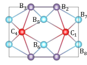
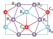
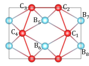
In this work we decipher the microscopic mechanism that determines the tilt parameter . For this purpose we focus on the SG number 59 that describes the structure 222The tilted Dirac cone has been experimentally observed in the so called structure of borophene Feng et al. (2017) of borophene Farajollahpour2019 ; Bradley and Cracknell (2010); Krowne and Sha (2021). But the logic employed here is generic and is applicable to other SGs, and can even be used to discover new examples of GQM. We show that in this structure, the low-energy and high-energy degrees of freedom are nicely separated into two sublattices denoted by gray and teal circles in Fig. 1(a), respectively. When the high energy sites available in this particular SG are integrated out, the underlying honeycomb lattice will be promoted to a ”honeycomb graph”. Molecular orbitals play significant role in attaching new ”graph edges” to the simple underlying honeycomb lattice. This graph has the ability to lead to a controlable tilt and hence spacetime structure in the long distance. On such a graph, even if instead of fermions one places a circuit, again a tilted Dirac cone can be obtained Motavassal and Jafari (2021). Therefore GQMs themselves can be emulated by circuits with a larger degree of tunability.
II Results and discussion
II.1 Protection of the Dirac node
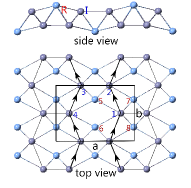
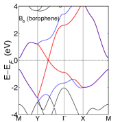
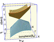
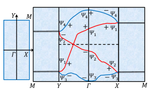
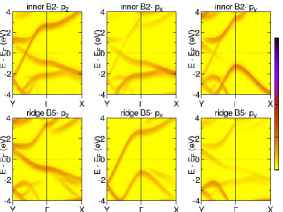
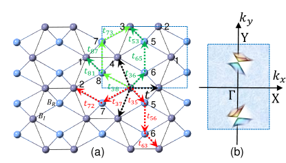
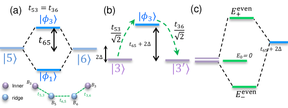
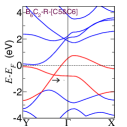
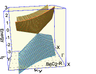
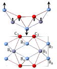
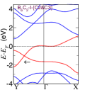
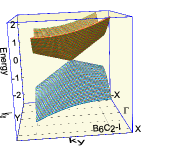
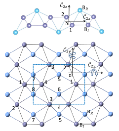
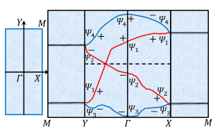
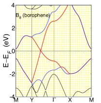
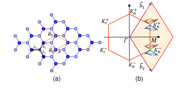
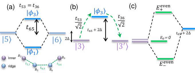
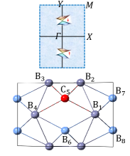
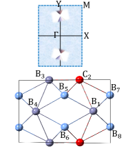
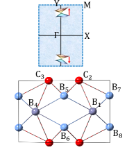
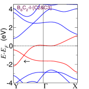
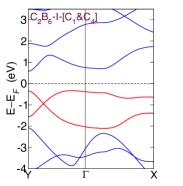
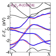
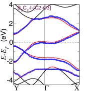
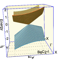
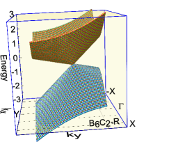
The relevant orbitals in the boron (as well as C) atom are orbitals. The possibility of formation of and hybridization establishes the honeycomb lattice Katsnelson (2012), and structures such as that involve buckled honeycomb networks as natural lattices for these atoms. As can be seen in Fig. 1(a), there is a backbone (buckled) honeycomb sub-lattice denoted with gray circles that are called inner (I) sites. The rest of the lattice sites are called ridge (R) sites and are denoted by teal circles. First principle calculations indicate that the resulting Dirac cone is tilted Zhou et al. (2014); Lopez-Bezanilla and Littlewood (2016) which is shown as red (low-energy) band in Fig. 1(b) and the three dimensional reconstruction of the band structure is shown in panel (c). The first thing that the SG implies about the tilted Dirac cone is that on the and lines in the border of the Brillouin zone (BZ) of Fig. 1(d), two bands ”stick together” (as Kittel puts it Kittel (i1987)) where the two-dimensional irreducible representations are protected by non-symmorphic elements Kittel (i1987). Then the compatibility relations gives the qualitative band picture of cat’s cradle shape Fan et al. (2018) shown in panel (d). For pedagogical details of the derivation of this figure with group theory methods see the supplementary information (SI).
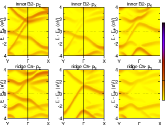
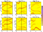
Of course the protection of the tilted Dirac cone by the underlying SG is interesting, but it is not essential for the main purpose of this paper, namely the ”tilt” of the Dirac cone. The symmetry considerations do not explain why and how the tilt parameter is formed. In order to ”manipulate” the tilt of the Dirac cone at will, one needs a microscopically detailed understanding of the root cause of formation of tilt in the Dirac cone. To achieve this, we need to identify the low-energy degrees of freedom that give rise to the tilted Dirac cone dispersion. For this purpose in Fig. 1(e) we have plotted an orbital projected representation of the band structure that resolve the contribution of atoms 2 (I) and 5 (R). As can be seen, the dominant contributions to the tilted Dirac dispersion comes from the orbitals of the I atoms (top left plot in panel (e)). The R atoms also contribute via their and orbitals (bottom left and center). The remaining two boxes on the top row indicate little contributions from the and orbitals of the I atoms that arises from the buckling of the honeycomb sublattice.
| (atomic) | ||||||||
|---|---|---|---|---|---|---|---|---|
| pure borophene | 2.09 | -2.66 | 2.09 | 2.09 | -1.87 | -1.87 | -1.87 | -2.54 |
| B6C2-I-[C2C3] | 1.93 | -2.52 | 1.96 | 1.92 | -1.52 | -1.52 | -1.55 | -2.34 |
| B6C2-R-[C5C6] | 2.14 | -2.33 | 2.12 | 2.15 | -2.23 | -2.21 | -2.20 | -2.43 |
| (renormalized) | ||||||||
| pure borophene | -2.21 | -2.36 | -1.07 | -1.99 | -2.51 | 0.46 | 0.48 | 0.49 |
| B6C2-[C2C3] | -2.37 | -1.75 | -0.95 | -1.62 | -2.05 | 0.36 | 0.66 | 0.47 |
| B6C2-R-[C5C6] | -2.05 | -2.49 | -1.09 | -2.24 | -2.85 | 0.59 | 0.32 | 0.66 |
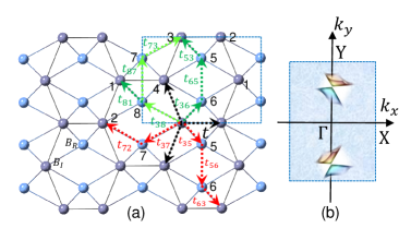
In panel (a) of Fig. 2 we have labeled atomic hopoings paths with green and red dashed lines that connect I sites by virtual hoppings through R sites. There is only first neighbor direct hopping between the I sites denoted by black arrows. The appropriate atomic orbitals involved in forming the above microscopic hoppings can be extracted from the DFT calculation. Working in a gauge that all ’s are real, the hermiticity implies . Panel (b) depicts the BZ of original lattice. The insight from the projected bands in the left and center columns in the second row of Fig. 1(e) is that both and orbitals of the R atoms are of comparable importance and must be incorporated into the atomic scale computation of the (dark green) and (light green). Similarly the first column of Fig. 1(e) suggests that the orbitals of R and I atoms dominate in hopping process. Tab. 1 shows the calculated values of these hopping parameters for pristine borophene (B8) and C-doped borophene B6C2 using Wannier function Mostofi ; Freimuth . The purpose of substituting C for B is to study its effect in the tilt of the Dirac cone. The substituted carbon dimers are placed in R and I positions, respectively. Using these parameters one can re-construct the ab initio bands with four orbitals of four inner sites, and eight and orbitals of ridge sites. The nice coincidence of the original DFT bands with Wannier-interpolated bands in Fig. S9 (see SI) shows that the obtained values are reliable and the used atomic orbitals are adequate.
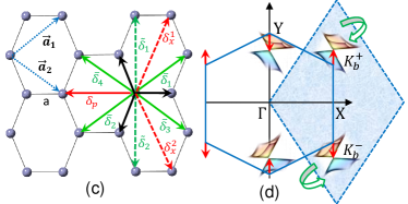
Although such a atomic picture might be satisfactory if one wishes to focus on the low-energy features of the tilted Dirac cone around the Fermi surface, but still working with a -band Hamiltonian is neither convenient, nor the essential long-range physics depends on so many short-distance details. To achieve an effective two-band model, we need to decimate the lattice into an effective honeycomb graph shown in Fig. 2(c) where two possible ways of representing its BZ are depicted in panel (d). On such a coarse-grained lattice, the virtual atomic hopping paths will be replaced by effective hoppings of the same color in panel (c). The connection between these effective hoppings and atomic hoppings is a nice example of renormalization that will be discussed now.
II.2 Renormalization via molecular orbitals:
Anderson in his book maintains that renormalization is one of the pillars of condensed matter physics Anderson (2018). In this section we will show that the same concept is encoded into a local quantum chemistry of the borophene in a remarkable way. Since we are not interested in higher energy features that take place away from the tilted Dirac node, we build an effective picture based on Fig. 2(c) where the ”effective” hoppings must be evaluated from the atomic scale data in the upper part of Tab. 1. The low-energy degrees of freedom are dominated by the orbitals of the I sites. So we decimate the lattice by elimination of the R sites. In doing so, the effective coarse-grained system becomes the honeycomb graph in Fig. 2(c). The nearest neighbor hoppings denoted by black arrows take place within the low-energy subspace and are responsible for the formation of a parent Dirac cone from the orbitals of the I sites. Slight anisotropy in the black arrows is known to shift the location of the Dirac cone Vozmediano et al. (2010) within the rhombus BZ of panel (d) that we ignore here. Green/red hopping processes are associated with the second/third neighbors of the honeycomb backbone that originate from the corresponding atomic process of panel (a) via the renormalization.
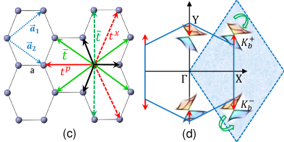
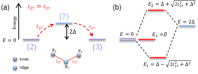
Let us see how the atomic processes in Fig. 2(a) are related to the effective hopping processes in Fig. 2(c). For example consider the simplest third neighbor R sites and of adjacent unit cells in Fig. 2(a) that becomes possible via atomic hoppings and of Fig. 2(a). The hopping process via the R site is depicted in Fig. 3(a). Assuming an on-site energy offset for the R sites with respect to I site, an electron starting at the site virtually hops to R site and then returns to low-energy sector at site . Through this process it gains the following energy
| (1) |
Even in the limit of this gives an energy lowering that can be regarded as effective hopping between the third neighbor sites and of the I sublattice. To intuitively understand this formula, note that in the absence of the I site, , and hence both even and odd combinations of third neighbor atomic orbitals remain inert. But once the inner site is present, the atomic hopping causes a coupling of with the even-parity state , leaving the odd parity state decoupled at zero energy. The coupling with the even parity combination provides a channel to lower the energy given by the effective hopping in Eq. (1). Furthermore, in the limit of the above formula reduces to the perturbatively appealing form . For pedagogical details of the above computation, please refer to section II of SI.
As a second example, consider the I site in Fig. 2(a) and the same site in the unit cell above it (that we denote by ). These sites will be second neighbor on the coarse grained lattice and there are two hopping pathways and connecting them that are denoted by light and dark green dashed lines in Fig. 2(a). The process of the calculation of the effective hopping amplitude is similar for the above two paths. So we focus on the first one. In principle one must consider the energy gained by the lowest molecular orbitals formed by the above chain of sites. This has been done in section III of SI. But the end result allows for a nice interpretation depicted in Fig. 4: First, due to hopping , the R sites and form bonding and anti-bonding molecular orbitals denoted by and in Fig. 4(a). Then as depicted in panel (b), an electron gains energy by virtually hopping via the anti-bonding orbital whose energy is now offset by . The hoppings connecting site and to are where the factor comes from the normalization . In the final step as shown in Fig. 4(c), the even-parity combination of and is mixed with to give an energy gain . A similar contribution arises from the second path. Adding the two contributions we obtain the total renormalized hopping of Fig. 2(c) as
In the above formula, the hopping parameters and are dominantly contributed by the and orbitals as the intensity of the orbitals in the second row of Fig. 1(e) is dominant, while is faint. Similarly the two other renormalized hopping parameters and can be computed. For details please refer to SI where we have shown that the elimination of higher energy states actually corresponds to the above simple molecular orbital analysis.
This is how the renormalized parameters of the coarse grained honeycomb graph model in the bottom part of Tab. 1 are computed from the ab initio data of the top part of the table. Note that if instead of structure, we had a simple honeycomb lattice (such as in graphene), such a large values of second or third neighbor hopping given in Tab 1 would be unthinkable as hopping between the atomic orbitals exponentially decays with distance. Therefore the virtual hopping via the ridge sites attaches a great importance to them as providers of channels for energy gain and ultimate formation of renormalized hoppings on a coarse grained lattice of inner sites. Furthermore, this is an example of how the molecular orbital play a significant role in the formation of longer range hoppings on the decimated lattice.
II.3 Effective coarse-grained model
Now that we have identified the orbitals residing at the inner sites as the low-energy degrees of freedom, and have computed various renormalized hoppings between second and third neighbors, we are ready to write down a physically clear low-energy effective model that will straightforwardly demonstrate how the renormalized parameters and can provide information about the position and the amount of the tilt.


The first neighbor hoppings denoted by black arrows in Fig. 2(c) and are present even when there are no R sites. In the two-dimensional Hilbert space of A and B sublattice of such a honeycomb lattice, these hoppings contribute the usual off-diagonal term to the Bloch Hamiltonian, where the sum over runs over three first neighbors in Fig. 2(c). This is responsible for the formation of a pair of upright Dirac cones similar to graphene. Slight anisotropy of the honeycomb lattice of R sites will amount to a shift in the location of the Dirac cone Vozmediano et al. (2010) which is irrelevant for our purposes. For concrete calculations, we assume a regular effective honeycomb lattice of bond length for which the Dirac nodes in the rhombus BZ are at Katsnelson (2012).
Next let us consider the third neighbor hoppings denoted by red arrows in Fig. 2(c) labeled by ( for pseudo, as they give rise to pseudogauge fields that shift the location of the Dirac node) and ( to emphasize the role of orbitals of R sites). They contribute another off-diagonal term denoted by to the Bloch Hamiltonian. Expanding this form factor around the Dirac nodes above, gives rise to (i) a shift of the Dirac node, where is the nearest neighbor hopping (assumed to be ) and (ii) anisotropy in the Fermi velocity given by and . Therefore the first and third neighbor hoppings establish the location of the (still upright) Dirac cone and determine its Fermi velocities.
Now let us focus on the second neighbors (green arrows) in Fig. 2(c) that are the root cause of the tilt formation Goerbig et al. (2008). Since these hoppings are driven via virtual hopping through different arrangements of molecular orbitals, there are two types of them denoted by solid () and dashed () green lines. These hoppings being second neighbor, connect two atoms on the same sublattice, and therefore contribute to the diagonal terms, namely and components of the effective Hamiltonian matrix. Among the matrices with , only and can contribute diagonal terms. So now one has to decide whether these diagonal terms come with the same sign ( term tilt) or opposite signs ( term gap). There are two ways to see that this term must be proportional to the : (i) Analysis of the irreducible representations and compatibility relations of the original structure in Fig. 1(d) shows that the crossing of the red bands is protected by the glide elements of the lattice (see SI for details). Since the effective theory has to obey this protection against gap opening, the term is ruled out. (ii) Consider the renormalized lattice itself and focus on the solid green line in Fig. 2(c). If the hopping between and in Fig. 1(a) contributes to AA term, the hopping between and contribute to BB term. Both these contributions arise from the orbitals of these atoms via intermediate hopping through orbital of atom . Apparently for orbitals the ”northwest” () and ”northeast” () hoppings are identical. Similar arguments holds for the dashed green line in Fig. 2(c). In this case AA (BB) term is generated by () path. Again the orbitals of the atoms symmetrically connect and (remember is the same as but in adjacent unit cell. Similarly for .), thereby giving identical AA and BB terms in the effective Hamiltonian.
Therefore the effective Hamiltonian becomes
| (3) | |||
Taylor expanding the diagonal term around the Dirac node formed by off-diagonal terms gives,
| (4) |
where corresponds to the valley around which the expansion is performed.
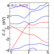
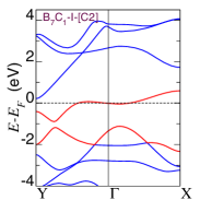
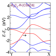
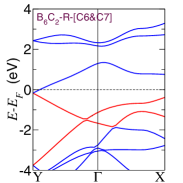
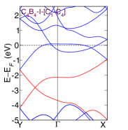
The above equation indicates that the tilt arises from the difference of the second neighbor hoppings and that in turn are generated via the and orbitals of the R atoms. An immediate suggestion of the above model is to (partially) replace the R-site boron atoms by carbon atoms to see whether the tilt is changed or not. In Fig. 5 we have replaced two of the boron atoms with C atoms. For this purpose there are two choices: (i) To place a carbon dimer on the R sites as in the panel (a) or (ii) to place the carbon atoms in the I sites as in panel (f). The results are summarized in Tab. 1. For case (i), the location of the Dirac node is shifted towards the pint and its tilt increases. Placing carbon atoms in the R sites shifts the and sites to higher energies, thereby generating larger and (see Tab. 1) that ultimately increases the tilt from the of the pristine borophene to in B6C2-R-[C5C6]. Our picture provides also a way to decrease the tilt parameter. In this case, the hybridization of the orbitals of sites with the R sites () reduces as in Tab. 1 and hence the resulting and likewise are scaled down, thereby reducing the tilt to in B6C2-I-[C2C3]. The above values of the tilt are calculated based on Eq. (4) and as detailed in SI are in good agreement with the corresponding values directly extracted from DFT bands.
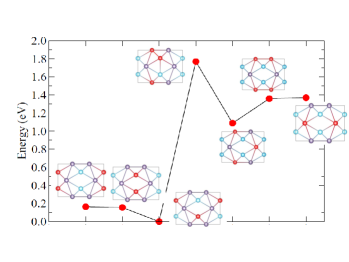
As shown in Fig. S6 of the SI, for doping of two carbon atoms into the structural unit of B8, the R-site configurations (c) and (k) have the lower energy than all other configurations, with staggered configuration (k) having slightly lower energy than (c). For a perfect (translationally invariant) doping of two C into the borophene structure, the changes in the tilt are discrete. However, the concentration of C atoms can be continuously varied. Statistical averaging for a concentration that continuously varies between and is expected to generate a continuously varying tilt. The dominant configurations will be the R-site dimers and staggered R-site configurations of panel (c) and (k) of Fig. S6. The lack of perfect backscattering of Dirac electrons is expected to protect the Dirac cone against the Anderson localization.
III Summary and outlook
Based on our ab initio calculations, we have identified the orbitals of the I sites as real space sublattice on which the low-energy degrees of freedom in lattice reside. The effective hoppings between these sites are obtained via renormalization that encodes the virtual hopping via R-sites. This gives a physically clear picture of the formation of the tilt in two-dimensional Dirac cone of borophene. In our picture, tilt arises from a competition between two renormalized hoppings and between the second neighbor I-sites. The former involves virtual hopping via two R sites (and orbitals of the R sites), while the later involves one R site. This builds in a natural difference between and . That is why the pristine borophene has a substantial tilting. Within this picture it is natural to expect that replacing the ridge (inner) atoms by C increase (decreases) the tilt. The rest of the effective hoppings determine the location of the (protected) Dirac node and the anisotropy in the Fermi velocity.
The logic of our work can be applied to other SGs to discover more GQM within a class of 2D materials that afford to provide a ”parent” upright Dirac cone Yekta and Coworkers (2021): Molecular orbitals in peculiar SGs can mediate longer range hoppings on a backbone lattice of Dirac fermions by promoting it to appropriate graph. The resulting graph in turn deforms the Minkowski spacetime of the Dirac fermions into a metric involving spatio-temporal elements. The ability to tune the tilt parameter is tantamount to controllability of the ensuing solid-state spacetime structure. Dirac materials subject to ”gravitational” (i.e. geometric) disorder Ghorashi et al. (2020); Davis and Foster (2021) find their salient materialization in the present context when the carbon is randomly substituted for boron. Assuming a doping fraction of carbon atoms that can be continuously tuned, the most favorable configurations for the C atoms are R-site dimers and staggered R-site (Fig. S6 (c) and (k), respectively). Random substitutions of this form is expected to lead to continuous variation of tilt as a function of . The absence of backscattering for Dirac fermions protect it against Anderson localization Amini et al. (2009).
The relation between certain graphs and their continuum limit as space geometries is well known Boettcher et al. (2020); Baek et al. (2009); Kollár et al. (2019). Our current results suggests a solid-state platform to promote a simple lattice that supports Dirac fermions into a rich graph where vierbeins can be attached to the Dirac fermions Yepez (2011); Hughes et al. (2013). This enriches the physics of Dirac materials and promotes them to GQMs where a variety of spacetime geometries can be fabricated that might not even have any analogue in the cosmos. On the 2D materials side, there will be a plenty of room to explore the effects of ”geometric” forces or even synthesise non-Abelian gauge fields Farajollahpour and Jafari (2020) that are likely to lead to better control in electronic/optical devices, as the effects of spacetime curvature Exirifard et al. (2021); Exirifard and Karimi (2021) can be much stronger GQMs. Furthermore, the geometry of our emergent spacetime in GQMs roots in the Coulomb forces that are much stronger than the gravitational forces. Furthermore, unlike the gravity, the Coulomb forces can be both attractive and repulsive. Therefore the geometric structure of GQMs seems to be much richer than the Einsten’s gravity. In three dimensional tilted Dirac/Weyl fermions the resulting geometric theory can be even more interesting: The fermions in such materials are chiral and hence a chiral geometric theory can be relevant to GQM. The developments in GQMs will allow us to emulate aspects of spacetime geometry that is not easily accessible in the cosmos. GQMs have a potential to equip Dirac fermions with types of vielbeins Yepez (2011) that are beyond the spatial veilbeins of the strain/dislocation paradigm Hughes et al. (2013).
References
- Inui et al. (1990) T. Inui, Y. Tanabe, and Y. Onodera, in Group Theory and Its Applications in Physics (Springer Berlin Heidelberg, 1990), pp. 234–258, URL https://doi.org/10.1007/978-3-642-80021-4_11.
- Girvin and Yang (2019) S. M. Girvin and K. Yang, Modern Condensed Matter Physics (Cambridge University Press, 2019).
- Ryder (1996) L. H. Ryder, Quantum Field Theory (Cambridge University Press, 1996), URL https://doi.org/10.1017/cbo9780511813900.
- Bradlyn et al. (2016) B. Bradlyn, J. Cano, Z. Wang, M. G. Vergniory, C. Felser, R. J. Cava, and B. A. Bernevig, Science 353, aaf5037 (2016), URL https://doi.org/10.1126/science.aaf5037.
- Ando (2011) T. Ando, Journal of Applied Physics 109, 102401 (2011), URL https://doi.org/10.1063/1.3575639.
- Tajima et al. (2006) N. Tajima, S. Sugawara, M. Tamura, Y. Nishio, and K. Kajita, Journal of the Physical Society of Japan 75, 051010 (2006), URL https://doi.org/10.1143/jpsj.75.051010.
- Goerbig et al. (2008) M. O. Goerbig, J.-N. Fuchs, G. Montambaux, and F. Piéchon, Phys. Rev. B 78, 045415 (2008), URL https://link.aps.org/doi/10.1103/PhysRevB.78.045415.
- Kajita et al. (2014) K. Kajita, Y. Nishio, N. Tajima, Y. Suzumura, and A. Kobayashi, Journal of the Physical Society of Japan 83, 072002 (2014), URL https://doi.org/10.7566/jpsj.83.072002.
- Farajollahpour et al. (2019) T. Farajollahpour, Z. Faraei, and S. A. Jafari, Physical Review B 99 (2019), URL https://doi.org/10.1103/physrevb.99.235150.
- Jalali-Mola and Jafari (2019) Z. Jalali-Mola and S. A. Jafari, Phys. Rev. B 100, 075113 (2019), URL https://link.aps.org/doi/10.1103/PhysRevB.100.075113.
- Verma et al. (2017) S. Verma, A. Mawrie, and T. K. Ghosh, Phys. Rev. B 96, 155418 (2017), URL https://link.aps.org/doi/10.1103/PhysRevB.96.155418.
- Jafari (2019) S. A. Jafari, Phys. Rev. B 100, 045144 (2019), URL https://link.aps.org/doi/10.1103/PhysRevB.100.045144.
- Westström and Ojanen (2017) A. Westström and T. Ojanen, Phys. Rev. X 7, 041026 (2017), URL https://link.aps.org/doi/10.1103/PhysRevX.7.041026.
- Liang and Ojanen (2019) L. Liang and T. Ojanen, Phys. Rev. Research 1, 032006 (2019), URL https://link.aps.org/doi/10.1103/PhysRevResearch.1.032006.
- Volovik (2016) G. E. Volovik, JETP Letters 104, 645 (2016), ISSN 1090-6487, URL https://doi.org/10.1134/S0021364016210050.
- Volovik (2018) G. E. Volovik, Physics-Uspekhi 61, 89 (2018), URL https://doi.org/10.3367%2Fufne.2017.01.038218.
- Nissinen and Volovik (2017) J. Nissinen and G. E. Volovik, JETP Letters 105, 447 (2017), ISSN 1090-6487, URL https://doi.org/10.1134/S0021364017070013.
- Mohajerani et al. (2021) A. Mohajerani, Z. Faraei, and S. A. Jafari, 33, 215603 (2021), URL https://doi.org/10.1088%2F1361-648x%2Fabe64e.
- Feng et al. (2017) B. Feng, O. Sugino, R.-Y. Liu, J. Zhang, R. Yukawa, M. Kawamura, T. Iimori, H. Kim, Y. Hasegawa, H. Li, et al., Phys. Rev. Lett. 118, 096401 (2017).
- Bradley and Cracknell (2010) C. Bradley and A. Cracknell, The mathematical theory of symmetry in solids: representation theory for point groups and space groups (Oxford University Press, 2010).
- Krowne and Sha (2021) C. M. Krowne and X. Sha, Materials Research Express 8, 026301 (2021), URL https://doi.org/10.1088/2053-1591/abdf7e.
- Motavassal and Jafari (2021) A. Motavassal and S. A. Jafari, Phys. Rev. B 104, L241108 (2021), URL https://link.aps.org/doi/10.1103/PhysRevB.104.L241108.
- Katsnelson (2012) M. I. Katsnelson, Graphene (Cambridge University Press, 2012), URL https://doi.org/10.1017/cbo9781139031080.
- Zhou et al. (2014) X.-F. Zhou, X. Dong, A. R. Oganov, Q. Zhu, Y. Tian, and H.-T. Wang, Phys. Rev. Lett. 112, 085502 (2014).
- Lopez-Bezanilla and Littlewood (2016) A. Lopez-Bezanilla and P. B. Littlewood, Phys. Rev. B 93, 241405 (2016), URL https://link.aps.org/doi/10.1103/PhysRevB.93.241405.
- Kittel (i1987) C. Kittel, Quantum Theory of Solids (John Wiley & Sons, New York, i1987), 2nd ed.
- Fan et al. (2018) X. Fan, D. Ma, B. Fu, C.-C. Liu, and Y. Yao, Physical Review B 98 (2018), URL https://doi.org/10.1103/physrevb.98.195437.
- Yekta et al. (2021) Y. Yekta, H. Hadipour, and S. A. Jafari, How to tune the tilt of a dirac cone by atomic manipulations? (2021), eprint arXiv:2108.08183.
- Mostofi et al. (2008) A. A. Mostofi, J. R. Yates, Y.-S. Lee, I. Souza, D. Vanderbilt, and N. Marzari, Comput. Phys. Commun 178, 685 (2008).
- Freimuth et al. (2008) F. Freimuth, Y. Mokrousov, D.Wortmann, S. Heinze, and S. Blugel, Phys. Rev. B 78, 035120 (2008).
- Anderson (2018) P. W. Anderson, Basic Notions of Condensed Matter Physics (CRC Press, 2018), URL https://doi.org/10.4324/9780429494116.
- Vozmediano et al. (2010) M. Vozmediano, M. Katsnelson, and F. Guinea, Physics Reports 496, 109 (2010), URL https://doi.org/10.1016/j.physrep.2010.07.003.
- Yekta and Coworkers (2021) Y. Yekta and Coworkers, In progress (2021).
- Ghorashi et al. (2020) S. A. A. Ghorashi, J. F. Karcher, S. M. Davis, and M. S. Foster, Phys. Rev. B 101, 214521 (2020), URL https://link.aps.org/doi/10.1103/PhysRevB.101.214521.
- Davis and Foster (2021) S. M. Davis and M. S. Foster, Geodesic geometry of 2+1-d dirac materials subject to artificial, quenched gravitational singularities (2021), eprint arXiv:2107.04047.
- Amini et al. (2009) M. Amini, S. A. Jafari, and F. Shahbazi, EPL (Europhysics Letters) 87, 37002 (2009), URL https://doi.org/10.1209/0295-5075/87/37002.
- Boettcher et al. (2020) I. Boettcher, P. Bienias, R. Belyansky, A. J. Kollár, and A. V. Gorshkov, Physical Review A 102 (2020), URL https://doi.org/10.1103/physreva.102.032208.
- Baek et al. (2009) S. K. Baek, P. Minnhagen, and B. J. Kim, Physical Review E 79 (2009), URL https://doi.org/10.1103/physreve.79.011124.
- Kollár et al. (2019) A. J. Kollár, M. Fitzpatrick, and A. A. Houck, Nature 571, 45 (2019), URL https://doi.org/10.1038/s41586-019-1348-3.
- Yepez (2011) J. Yepez, arXiv preprint arXiv:1106.2037 (2011), URL https://arxiv.org/abs/1106.2037.
- Hughes et al. (2013) T. L. Hughes, R. G. Leigh, and O. Parrikar, Phys. Rev. D 88, 025040 (2013), URL https://link.aps.org/doi/10.1103/PhysRevD.88.025040.
- Farajollahpour and Jafari (2020) T. Farajollahpour and S. A. Jafari, 2 (2020), URL https://doi.org/10.1103%2Fphysrevresearch.2.023410.
- Exirifard et al. (2021) Q. Exirifard, E. Culf, and E. Karimi, Communications Physics 4 (2021), URL https://doi.org/10.1038%2Fs42005-021-00671-8.
- Exirifard and Karimi (2021) Q. Exirifard and E. Karimi, Schrödinger equation in a general curved space-time geometry (2021), eprint arXiv:2105.13896.
Supplemental materials to the manuscript: Tunning the tilt of a Dirac cone by atomic manipulations: application to 8Pmmn borophene
Since we expect dual readership both from condensed matter and gravity research, in this supplementary information (SI), we provide pedagogical derivations of all the relations and figures referred in the text. To benefit the graduate students, this SI is meant to make the paper self-contained, and understandable on its own trying to minimize consultation with other references.
IV Symmetry analysis
In this section, we illustrate the application of group theory methods in classification and labeling of the band structures by way of example of borophene. This section is based on chapter 10 of C. Kittel’s Quantum Theory of Solids Kittel . For a quick and concise introduction to the theory of groups and their representations, we recommend chapter 3 of G. Mahan’s Applied Mathematics Mahan .
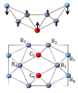
Here, the two-dimensional rectangular lattice of pristine borophene B8 has symmetry group of . The crystal structure of the pure borophene and the character table for the D2h () point group are presented in Fig. S1(a) and Table 2 respectively Dresselhaus ; Bradley-1 . The generators of space-group are given by two screw operations and together with an inversion operation , where () is a nonsymmorphic operator meaning the twofold rotation () around the () axis is followed by a translation () as indicated in Fig. S1(a). Note that the inversion center is located at the crossing point of two screw axes (between bond line of atom 1 and 2) as depicted in Fig. S1(a) and the screw is performed around this inversion center. These three independent operations can produce all other symmetry operations of the space group as follow:
| (S1) |
Without taking the spin of the electrons into account, () group has eight 1D irreducible representations given in character Table 2. There are two other 2D representations belonging to the double group (i.e. accounting for both orbitals and spin) which is considered in presence of spin-orbit coupling and is not indicated in this table.
First of all, following Kittel Kittel we establish that the non-symmorphic elements and that are combination of two-fold rotations around the axis indicated in Fig. S1(a) followed by half-cell translation, guarantee the ”sticking together” of the bands along the Brillouine zone (BZ) boundary as indicated in Fig. S1(b). Then we show that band inversion happens by connecting two eigenvalues of these operators, as a result of which a Dirac point between and is protected by the screw axis operator , in agreement with our ab initio band structure, as shown in Fig. S1(c).
Suppose that is a solution of the wave equation at -point along boundary of the BZ (i.e. or line). The screw rotation , mirror , and inversion operations transform the wave function according to , , and respectively which result in , or the multiplication rule . Other multiplication rules similarly follows.
Now to prove that along the line defined by , there is a double degeneracy, we show that , , and satisfy the algebra of Pauli matrices. The definition of implies ( is the length of the unit cell in direction)
| (S2) |
where, in the the third equality have used the Bloch theorem and in the fourth equality we have used that on line we have .
Subsequently, from the definition of and , We have and . Then by multiplying these operators two by two, we find their anticommunication relations as follows:
| (S3) | |||
| (S4) |
which indicate that along the line defined by , it gives anticommunication relation .
For and operators, the same procedure yields
| (S5) | |||
| (S6) |
where again along the line, we have .
Finally, considering and operators results in
| (S7) | |||
| (S8) |
which implies along the line defined by .
Naming , , and , we find that , , and obey the Clifford algebra defined by anticommutation relations: where is the identity matrix and is the Minkowski metric. As is well known the representations of the above algebra are even dimensional, the lowest dimensional representation of which will be two-dimensional where matrices will be represented by Pauli matrces as e.g. . Therefore along the , the bands are at least doubly degenerate. Similar arguments applies to three operators and along the direction.
Now let us see how the degeneracies can split by moving along the path. For this we need to label the eigenstates at the point in terms of the eigenvalues of . Since the states of inner sites in backbone honeycomb sub-lattice are responsible for formation of Dirac cone, the most generic molecular orbitals or Bloch states at the vicinity of point composing the bottom of conduction band and and those at the top of valence band and can be constructed from the binding (anti-binding) combinations and of the and bonds, respectively as,
| (S9) | |||
| (S10) |
Note that the above ordering that places and at the bottom of conduction band can be obtained from a simple tight binding (molecular) picture involving atoms in Fig. S1(a). Likewise, it is quite reasonable to place (the most ”even” combination of atomic orbitals with no minus sign) at the lowest energy, followed by at slightly higher energy. Now we apply the action of the point group elements on this molecular orbitals to construct the elementary band representation. As depicted in Fig. S1(a), replaces the site numbers as and . Moreover, the orbitals having character, change sign under a rotation around (as well as rotation around ). Therefore the effect of on the above wave functions becomes
| (S11) |
Similarly for the action of we have and , followed by (again since orbital has character). Therefore its effect on the above four states becomes
| (S12) |
The effect of operator on the above wave functions are the same as . The eigenvalues of operators , , and for bottom of conduction and top of valence band states (+1,+1,+1) and (+1,-1,-1) respectively in agreement with Ref. Fan ,
| Rep | ||||||||
|---|---|---|---|---|---|---|---|---|
| 1 | 1 | 1 | 1 | 1 | 1 | 1 | 1 | |
| 1 | 1 | 1 | 1 | -1 | -1 | -1 | -1 | |
| 1 | 1 | -1 | -1 | 1 | 1 | -1 | -1 | |
| 1 | 1 | -1 | -1 | -1 | -1 | 1 | 1 | |
| 1 | -1 | 1 | -1 | 1 | -1 | 1 | -1 | |
| 1 | -1 | 1 | -1 | -1 | 1 | -1 | 1 | |
| 1 | -1 | -1 | 1 | 1 | -1 | -1 | 1 | |
| 1 | -1 | -1 | 1 | -1 | 1 | 1 | -1 |
Now we need all the possible paths where the crystal symmetries connect bands with corresponding eigenvalues of the above three operators in a consistent way. Compatibility relations Kittel express that the irrepresentation along the high-symmetry lines are completely determined by the irrepresentation that appear at high-symmetry points (little groups of high-symmetry points/lines). We apply it to the line and according to the Eqs. (S11) and (S12). Taking one possible path as an example, as shown in Fig. S1(b) for , one of the conduction bands from point (the eigenfunction of with eigenvalue of +1) is connected to the point (the eigenfunction of with eigenvalue of +1), and then inverted with the valence band from point (the eigenfunction of with eigenvalue of +1) that gives (tilted) cone crossing along the path when we consider the same procedure for .
For the formation of cone crossing a ”sticking together” (as Kittel puts it) of conduction states and valence states is necessary. Such sticking together is protected by glid/screw elements Kittel . In our case it is the screw-symmetry . Other possibilities are to have the crossing along the path, or to have a crossing between the blue and red bands of Fig. S1(b). These possibilities for band inversion between states with is ruled out by the specific ordering given in Eqs. (S9) and (S10).
V 8Pmmn motivated Tight-binding model for tilted Dirac fermions
As pointed out in the main text, effective degrees of freedom are orbitals of inner sites the projection of which on the plane will be a honeycomb lattice. In this effective model, the buckling of honeycomb lattice sites are ignored. This can be absorbed into effective hybridization with orbitals of the ridge sites. Furthermore, the projection of the inner sites of lattice into plane will not be a regular honeycomb lattice. Ignoring this will amount to a shift in the location of the Dirac node. This shift can also be absorbed into various effective hoppings. Therefore for modeling purposes, it is enough to start with an ”effective regular honeycomb lattice” on which the relevant degrees of freedom (the orbitals of the inner sites) reside. In this section we pedagogically derive all the details related to the formation, movement and titling of the Dirac cone based on the effective honeycomb lattice. As is shown in the main text, the picture arising from an effective model can accurately reproduce the DFT tilt parameters. Furthermore, having a tight binding two-band model allows to study various effects such as disorder/interactions/symmetry breaking.
V.1 Theory without ridge atoms
Without ridge atoms (faint teal sites in Fig. 1(a) and Fig. 2(a) of the main text), life is simple and one basically needs a theory of graphene which will be pedagogically and quickly reviewed below to build upon. We therefore start with Fig. S2 that depicts a regular honeycomb lattice and its associated first Brillouin zone.
The three vectors connecting every site from a given sublattice to three nearest neighbors from the opposite sublattice in Fig. S2(a) are
The primitive lattice basis vectors are
Using gives the following basis for the reciprocal space,
where is the distance between two neighbouring atoms. In the hexagonal Brillouin zone it appears the there are six corners . But in in fact two of them are independent and fall into two categories related to each other by a reciprocal lattice vector constructed from the above vectors. For example the corners of Brillouin zone shown in Fig. S1(b) labeled by and are given by,
As can be seen adding to gives and hence they are equivalent. Similarly and are equivalent. So in the calculations, one can pick a convenient one. The effective theories around equivalent points are the same within a gauge transformation that will be discussed below. The points indicated in the rhombic Brillouin zone of Fig. S2(b) manifestly emphasizes that there are two independent corners that can not be connected to each other by a reciprocal lattice vectors.
Denoting by the field operators for the annihilation of electrons in orbitals of the and sublattices of the honeycomb lattice, the parent Hamiltonian is basically the theory of graphene and is given by,
Fourier transformation of the above Hamiltonian becomes,
that begs for a matrix representation as
This is how the spinor structure emerges. The form factor connects the opposite sublattices, and hence is off-diagonal in the above sublattice space and is given by,
Plugging in the Cartesian representations of , , and given above and carrying out the summation over the three neighbors, the famous formula of graphene literature can be obtained,
The above form factor vanishes at the corners of the hexagonal Brillouin zone. Expanding it around two independent corners, e.g. gives,
The overall factor of can be gauge transformed by rotating the overall phase of the wave function in one sublattice. For example gauge transforming the amplitude of wave function on sublattice as , eliminates the factor above and we have
Upon the above gauge transformation the behavior of the Hamiltonian around the crossing points is given by,
Defining , this formula gives two representations of the Dirac theory with and , hence massless Dirac electrons. These two representations are connected to each other by time-reversal operator followed by where is complex conjugation.
V.2 Role of ridge atoms
The borophene’s lattice consists of two different types of B atoms, which we will call inner B (BI) and ridge B (BR) atoms in Fig. S3(a). The BI atoms form a hexagonal graphene-like lattice and BR atoms look like one-dimensional chains passing through the effective honeycomb lattice as in Fig. S3(c). As pointed out, in absence of BR atoms, the structure looks like a distorted graphene lattice. This lattice naturally includes the nearest neighbor (black path hoppings in panel (c)) that gives rise to two Dirac cones described above. Deviations of the honeycomb lattice from planar structure allows for mixing with orbitals of the ridge sites, while the deviations of the projected honeycomb lattice from perfect symmetry of graphene accounts for shift in the location of the Dirac cones. Therefore the schematically depicted Dirac cones in panel (d) above are shifted and tilted as described below to form the two Dirac cones in panel (b) of the original lattice.
If there were not ridge sites, in a pure honeycomb lattice, hoppings between 2nd and 3rd neighbors via atomic orbitals would be negligibly small. Therefore there would be no green and red hoppings as in panel (c). However, ridge atoms provide dotted hopping paths of panel (a) that facilitate a hopping between 2nd and 3rd neighbors of the parent honeycomb-like lattice via virtual hopping through the ridge atoms. The connection between the microscopic paths in (a) and effective hoppings in (c) will be discussed in next section. For the purpose of present sub-section, we only need to focus on the effective green and red hoppings in panel (c) above. The corresponding hoppings as depicted in Fig. 2(c) of the main text are and for the green path (2nd neighbor). Two different symbols correspond to two different virtual processes depicted in panel (a) above. Similarly for the red paths there are two hoppings and as depicted in Fig. 2(c) of the main text. As we will see shortly, (and acts like a pseudo-gauge field that shifts the location of the Dirac cone. The superscript in is meant to emphasize a special role played by the orbitals of the ridge atoms that will be discussed in the next section. The and being 3rd neighbor hoppings connect a site from A sublattice to a one in the B sublattice. Therefore the corresponding form factor will contribute off-diagonally to the effective Hamiltonian. Furthermore, the hoppings and being 2nd neighbor hoppings connect atoms on the same site, and therefore the corresponding form factors and contribute diagonally to the effective Hamiltonian in the sublattice space. So we end up with
where provides a upright Dirac cone to begin with (as discussed in the previous sub-section).
Using the third nearest-neighbor vectors , , where ”” is an ”effective” lattice constant for the parent honeycomb lattice, the form factor and its Taylor expansion near the Dirac crossing become,
As can be seen the difference between the 3rd neighbor hoppings generated via two different microscopic paths effectively shifts the of the opposite valleys by opposite values. Furthermore, the coefficients of the and above that arise from and contribute to the re-definition and anisotropy of the Fermi velocity. Remembering to affect the gauge transformation of the previous sub-section, the off-diagonal form factor giving still an upright (but shifted) Dirac cone becomes,
| (S13) |
This form makes it manifest how the third neighbor hoppings shift the Dirac cones and make their velocities anisotropic. The difference is responsible for the mutual movement of the Dirac cones alone the direction: The Dirac point at move downward by and Dirac point at move upward by the same value. An illustration of this shift is indicated in Fig. S3(d) by red arrows. So, by increasing difference , the Dirac-nodes at move toward . Equivalently, this means that the Dirac-nodes at move away from as indicated by red arrows.
Formation of the tilt: We are now ready to discuss the green path hoppings in Fig. S3(c) that are second neighbor hoppings on the effective honeycomb structure. The form factors and correspond to the real-space displacements
and,
respectively. The , , in the diagonal part of Hamiltonian are thus
that add up to give a tilt form factor,
Expanding around the Dirac point , the total AA matrix element becomes,
| (S14) |
Note that the BB matrix element is the same as above. Remember that the gauge transformation does not change the BB matrix element as a factor gives . From the above formula we read:
| (S15) |
Eqs. (S13) and (S15) derived for our model system are great guiding principles. Eq. (S13) shows that the 3rd neighbor (red) hoppings are responsible for the location and anisotropy of the upright Dirac cone. Eq. (S15) simply means that the tilt (a long distance property) depends on the difference between the microscopic parameters , namely the difference in the hopping via two different green paths in Fig. S3(c). This model shows how the presence of ridge atoms move and tilt the Dirac cone. In the following section we are going to show how the effective hoppings in panel (c) of Fig. S3(c) arise from microscopic hoppings in panel (a).
VI Effective hopping terms: renormalization via molecular orbitals
If one considers the honeycomb-like structure formed by inner sites only, the hopping between 2nd and 3rd neighbors are quite negligible. This is because in a tight-binding approach, the overlap between the atomic orbitals exponentially decays with the distance. But when the ridge sites (denoted by teal color in Fig. S3(a)) are added, they act as virtual sites thorough which a renormalized hopping between the () atomic orbitals of the inner sites is formed. In this section we provide a simple picture of renormalization based on the molecular orbitals theory that explains why relatively large hoppings between 2nd and 3rd neighbors are obtained. The remarkable agreement of the tilt parameters extracted within such a local quantum chemistry picture indicates its validity. So in this section using molecular orbital theory, we first analytically derive these renormalized hopping parameters of new effective honeycomb lattice in term of hopping parameters of original lattice. This will show that the ridge atoms (BR) play a crucial role in mediating strong hoppings between the 2nd and 3rd inner sites atoms. Then we discuss the connection between the present molecular orbital treatment with a picture of renormalization procedure by considering Dyson equation for the local quantum clusters of the lattice.
Formation of effective third neighbor hopping: Let us illustrate the basic principle by considering inner sites B2 and B3 in Fig. S3(a) and see how the ridge site B facilitates a hopping between them. In Fig. S4(a) we have depicted an energy diagram where sites B2 and B3 (by symmetry) are at the same atomic energy levels and , respectively. The site B7 is assumed at state energetically lying above the inner sites. The atomic hopping and connecting sites B2 and B3 to site B7 that can be derived from Wannier states are indicated. These two (real) hoppings are the same by symmetry. The basic principle can be seen in the limit where . In this limit a virtual second order in hopping via higher energy atomic orbital stabilizes the energy of the states and by . The factor comes from two different ways of performing such a virtual process: and . The analytical extension of this result to arbitrary is straightforward.
In Fig. S4(b) we have denoted the energy level and of the inner and atomic sites before the hybridization by red and teal colors. The sites B2 and B3 are equivalent and hence symmetry adopted basis based on the even and odd representation of a two-element group including identity operation and operator that exchanges B2 and B3 is given by,
The states and are even parity and mix with each other by atomic hopping , while the state being odd parity decouples from the others. In fact state is a bonding (anti-bonding) molecular orbital and is composed of atomic orbitals of inner sites B2 and B3. The matrix elements and Hamiltonian in this basis are
that give,
As can be seen when , the bonding/anti-bonding states have zero energy (equal to the energy of atomic orbitals and ) and hence bonding/anti-bonding degrees of freedom are inert in this limit. Upon turning on the atomic hopping to ridge site B7, the above structure of the Hamiltonian, still leaves the anti-bonding orbital decoupled and hence it remains at zero energy, while the bonding (even parity) combination is mixed with giving rise to two split-off states at energies . The energy of the state is always less than energy of the original B2 and B3 sites. In the low-energy sub-space that – involving only the inner sites B2 and B3 – the high-energy site B7 is eliminated (or integrated out in the renormalization group terminology), this lowering of energy can be interpreted as an effective hopping between B2 and B3, namely,
| (S16) |
This is so, because in a sub-space composed of only inner orbitals and , placing such a off-diagonal hopping between the two states at energy zero, correctly reproduces the energy lowering of with respect to . This effective hopping in the main text has been denoted by and is responsible for a pseudo-gauge field that shifts the location of the Dirac node. Note that the in the limit, the above espression reduces to the perturbative result cited above, while in the opposite limit it becomes .
Formation of effective second neighbor hopping: As a second example of how longer range hoppings on the parent honeycomb-like lattice of inner atoms are formed, let us consider in Fig. S1(a) the effective hopping between site B3 in one unit cell and the same B3 in the lower unit cell (let’s call it ). This process will be achieved by two virtual paths: and . Let us consider the first virtual path indicated by dotted green path in Fig. S3(a). Denoting by and the atomic orbitals on the two B3 sites, and by and the atomic orbitals on the intermediate B5 and B6 sites, respectively, the four dimensional Hilbert space is broken into even sector
and odd sector
The hopping matrix elements between the atomic orbitals are shown in Fig. S5 and by symmetry . The hopping between B5 and B6 is associated with a -bonding between the orbitals of these two sites. Taking the energy offset for the ridge sites with respect to the inner sites into account, the even block of the Hamiltonian and its eigenvalues become,
while for the odd sector we have
In fact replacement maps the odd sector to even sector. This can be interpreted as the fact that the even sector take advantage of the hopping term between the atomic orbitals of the ridge atoms and generate larger stabilization. Therefore for the path, a contribution to the effective second neighbor hopping between the two B3 inner sites will become,
| (S17) |
A similar contribution arises from the path by simply replacing that gives
| (S18) |
Adding these two terms gives the green in Fig. 2(c) of the main text,
| (S19) |
It is rather surprising to note that the Eq. (S17) for the virtual hopping path can be obtained by a simple intuitive picture as follows: As shown in Fig. S5(a), first an antibonding orbital from the ridge sites B5 and B6 is formed that has been denoted by . The upward shift of the antibonding orbital with respect to the initial level of the ridge atoms is given by the off-diagonal element in the space of and . Then will have hopping matrix elements and to sites and , respectively. Then a virtual hopping with these amplitudes via the intermediate state at energy , precisely gives Eq. (S17).
Relation with renormalization: Now we are ready to show that the effective hoppings obtained in this way, admit a nice interpretation in terms of renormalization. As an example, let us elaborate on Eq. (S16) and show that it can be alternatively obtained from a renormalizatioin picture. This will establish that the molecular orbital theory that was explained in the previous part is indeed equivalent to a renormalization procedure.
Imagine the situation we discussed for effective third neighbor hopping energy between B2 and B3. Denoting as before the atomic basis , , and , and breaking the three dimensional Hilbert space into a two dimensional subspace composed of low-energy states , and a one-dimensional high energy subspace described by , the Hamiltonian can be split as,
where the subscripts L (H) stand for low-energy (high-energy) sectors. As described in the textbook of Grosso and Pastori Paravicini Grosso, the application of Dyson’s equation leads to a renormalized (effective) Hamiltonian in the low-energy subspace of the following form,
that depends on energy. Plugging the various sub-matrices in the above equation gives,
Now we have to evaluate the operator, whose matrix elements are energy-dependent as,
The eigenvalues are given by,
that immediately becomes,
This is exactly the result (S16) of our simple molecular orbital theory. The same logic applies to all other effective hoppings. Therefore the process of virtual hopping via the inner sites that involves molecular orbitals is actually equivalent to formation of renormalized hoppings in the low-energy sector of the theory (residing on the inner sites) as a result of elimination of higher-energy degrees of freedom that reside on ridge sites.
VII Ab initio calculation: relaxation, electronic structure, and stability
The crystal structure of pure borophene is presented in Fig. S1(a). The basic unit cell is rectangular and contains eight B atoms. For DFT calculation we use pseudopotential Quantum Espresso code Espresso based on plane wave basis set within the GGA in the Perdew-Burke-Ernzerhof (PBE) parameterization Perdew . Simulation of borophene rectangular unit cells is based on the slab model having a 25 vacuum separating slabs. We also consider monolayer of structure, where some of the B atoms are substituted by C atoms in the form of B8-xCx (=0, 1, 2). The obtained structural properties after the ionic relaxations such as lattice parameters, , , and component of the B and C atoms in crystal coordinates are shown in Table 3 for pure borophene (B8) and C-doped systems B8-xCx. We have depicted the crystal structure for situation where a single B atom in the ridge (inner) sites is replaced by C atom, denoted by B7C1-R-[C5] (B7C1-I-[C2]) in Fig. S6(a) (Fig. S6(b)). An interesting situation where a dimer of B atoms in ridge (inner) sites is replaced by a dimer of C atoms are denoted by B6C2-R-[C5C6] and B6C2-R-[C7C8] (B6C2-I-[C2C3] and B6C2-R-[C1C4]) and are shown in Fig. S6(c) and Fig. S6(d) (Fig. S6(i) and Fig. S6(j)). For completeness all inner B atoms are replaced by C atoms which are denoted by B4C4-R-[C1-C4]. The uniform -point grids of 24241 are used for the self-consistent field calculations of all systems. The Kinetic energy cut-offs for the wavefunctions and the charge density are and eV, respectively. For each systems, the Broyden-Fletcher-Goldfarb-Shanno quasi-Newton algorithm is used to relax the internal coordinates of the B and C atoms and possible distortions with convergence threshold on forces for ionic minimization as small as 10-4 eV.
| (1) | B8 [borophene] | (2) B7C1-R-[C5] | (3) | B7C1-I-[C2] | ||||||||
|---|---|---|---|---|---|---|---|---|---|---|---|---|
| =4.5210 | =3.2620 | =26.0 | =4.5686 | =3.2297 | =26.0 | =4.5191 | =3.2714 | =26.0 | ||||
| atom | atom | atom | ||||||||||
| B1 | -0.1850 | 0.5000 | -0.4841 | B1 | -0.1864 | 0.5120 | -0.4831 | B1 | -0.1757 | 0.5000 | -0.4872 | |
| B2 | -0.3150 | 0.0000 | 0.4841 | B2 | -0.3169 | 0.0333 | 0.4880 | C2 | -0.2991 | 0.0000 | 0.4832 | |
| B3 | 0.3150 | 0.0000 | 0.4843 | B3 | 0.3169 | 0.033 | 0.4810 | B3 | 0.3385 | 0.0000 | 0.4854 | |
| B4 | 0.1850 | 0.5000 | -0.4843 | B4 | 0.1864 | 0.5120 | -0.4841 | B4 | 0.1982 | 0.5000 | -0.4852 | |
| B5 | 0.5000 | 0.2476 | -0.4578 | C5 | 0.5000 | 0.2091 | -0.4527 | B5 | 0.5000 | 0.2470 | -0.4420 | |
| B6 | 0.5000 | -0.2476 | -0.4578 | B6 | 0.5000 | -0.2922 | -0.4537 | B6 | 0.5000 | -0.2470 | -0.4450 | |
| B7 | 0.0000 | 0.2532 | 0.4578 | B7 | 0.0000 | 0.2451 | 0.4574 | B7 | 0.0000 | 0.2470 | 0.4460 | |
| B8 | 0.0000 | -0.2532 | 0.4578 | B8 | 0.0000 | -0.2559 | 0.4594 | B8 | 0.0000 | -0.2470 | 0.4440 |
| (4) | B6C2-R-[C5C6] | (5) | B6C2-R-[C7C8] | (6) | B6C2-I-[C1C4] | |||||||
|---|---|---|---|---|---|---|---|---|---|---|---|---|
| =4.2809 | =3.5399 | =26.0 | =4.3721 | =3.5053 | =26.0 | =4.4132 | =3.1501 | =27.0 | ||||
| atom | atom | atom | ||||||||||
| B1 | -0.2116 | 0.5000 | 0.5326 | B1 | -0.2095 | 0.5000 | -0.4713 | C1 | -0.1924 | 0.5000 | -0.4863 | |
| B2 | -0.3228 | 0.0000 | 0.4716 | B2 | -0.3218 | 0.0000 | 0.4743 | B2 | -0.3133 | 0.0000 | 0.4866 | |
| B3 | 0.3228 | 0.0000 | 0.4716 | B3 | 0.3218 | 0.0000 | 0.4723 | B3 | 0.3133 | 0.0000 | 0.4866 | |
| B4 | 0.2116 | 0.5000 | 0.5326 | B4 | 0.2095 | 0.5000 | -0.4703 | C4 | 0.1924 | 0.5000 | -0.4863 | |
| C5 | 0.5000 | 0.8049 | 0.5347 | B5 | 0.5000 | 0.1970 | -0.4613 | B5 | 0.5000 | 0.2528 | -0.4475 | |
| C6 | 0.5000 | 0.1950 | 0.5347 | B6 | 0.5000 | -0.1970 | -0.4611 | B6 | 0.5000 | -0.2528 | -0.4485 | |
| B7 | 0.0000 | 0.7399 | 0.4609 | C7 | 0.0000 | 0.2721 | 0.4619 | B7 | 0.0000 | 0.2457 | 0.4452 | |
| B8 | 0.0000 | 0.2600 | 0.4609 | C8 | 0.0000 | -0.2721 | 0.4619 | B8 | 0.0000 | -0.2457 | 0.4482 |
| (7) | B6C2-I- [C2C3] | (8) | B6C2-R-[C6C7] | (9) | B4C4-I-[C1-C4] | |||||||
|---|---|---|---|---|---|---|---|---|---|---|---|---|
| =4.1139 | =3.1369 | =26.0 | =4.4473 | =3.2116 | =26.0 | =4.2279 | =3.2260 | =27.0 | ||||
| atom | atom | atom | ||||||||||
| B1 | -0.2061 | 0.5000 | 0.5104 | B1 | -0.1961 | 0.5000 | 0.5226 | C1 | -0.1966 | 0.5000 | -0.4849 | |
| C2 | -0.3167 | 0.0000 | 0.4744 | B2 | -0.3038 | 0.0000 | 0.4774 | C2 | -0.3033 | -0.0000 | 0.4849 | |
| C3 | 0.3167 | 0.0000 | 0.4744 | B3 | 0.3038 | 0.0000 | 0.4774 | C3 | 0.3033 | -0.0000 | 0.4849 | |
| B4 | 0.2061 | 0.5000 | 0.5104 | B4 | 0.1961 | 0.5000 | 0.5226 | C4 | 0.1966 | 0.5000 | -0.4849 | |
| B5 | 0.5000 | 0.7383 | 0.5630 | B5 | 0.5000 | 0.8024 | 0.5375 | B5 | 0.5000 | 0.2571 | -0.4423 | |
| B6 | 0.5000 | 0.2616 | 0.5630 | C6 | 0.5000 | 0.3041 | 0.5545 | B6 | 0.5000 | -0.2571 | -0.4423 | |
| B7 | 0.0000 | 0.7455 | 0.4520 | C7 | 0.0000 | 0.8041 | 0.4454 | B7 | 0.0000 | 0.2429 | 0.4424 | |
| B8 | -0.0000 | 0.2544 | 0.4520 | B8 | 0.0000 | 0.3023 | 0.4624 | B8 | 0.0000 | -0.2429 | 0.4424 |
As we have shown in the main text and the previous sections of SM, the formation of the Dirac nodes is controlled by those atoms residing at the inner sites, while the location and tilting properties are controlled by the atoms residing at the ridge sites. With the aim of finding new materials with tilted Dirac cone, as well as, in order to confirm our analytical model, in this section we investigate whether and to what degree the location and tilt of Dirac-cone would change if boron atoms replaced by another atoms like carbon. We establish that the coarse grained honeycomb lattice of tilted Dirac fermions presented in the main text, is fully supported by ab initio calculations.
For instance, for the case of substitution of single C atom in ridge sites B7C1-R-[C5], we obtain that lattice parameters and position of atoms are not too different from the pure B8 (borophene) and, as a consequence, the shape of band structure including location and tilt of Dirac-cone does not change much (see second part of Table 3 and Fig. S6(e)). On the other hand, the situation is different in the case of substitution of single C atom in inner sites, B7C1-I-[C2] due to the breaking of and symmetries (it breaks C2z and inversion symmetries when we consider effective hexagonal lattice). So, single C atoms in hexagonal lattice gap out the tilted Dirac cone bands, as presented in Fig. S6(f). This observation confirms that the atoms at the inner (honeycomb-like) sites are responsible for the formation of the parent Dirac-cone.
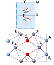
In the following, we will consider the situation in which a dimer of B atoms in the ridge (inner) sites is replaced by C atoms B6C2-R (B6C2-I). In the case of B6C2-R-[C5C6], Table 3 indicates that atoms in ridge sites get closer to the inner atoms in hexagonal lattice. As a result, the ratio between the effective hopping energy differences and the first neighbor hopping , namely and (that according to our model in section V of SM, control location and tilting of the Dirac cone, respectively) are expected to be larger than pure borophene. The movement of Dirac cones can be qualitatively seen in panel (g) and (m) of Fig. S6 where a dimer of C atoms are replacing the corresponding B atoms on the ridge sites. A weaker movement can be seen in panel (a) as only one C has been replaced in the ridge site, and hence a weaker shift in the ratio . Fig. S6(m) for B6C2-R-[C7C8] indicates that more or less the same story hold when we replace B7 and B8 by C atoms. There is another configuration of two C atoms in the ridge sites B6C2-R-[C6C7] (see Fig. S6(k)) which is energetically favorable as shown in Fig. S7, but it does not have significant value of tilt. Now let us consider the opposite case, displayed in panel (d) and (h) of Fig. S6 where the C dimers replace B dimers on the inner sites, namely B6C2-I-[C2C3] and B6C2-I-[C1C4]. In these cases the ridge atoms move away from the plane (see Table 3), thereby giving rise to opposite effect of panel (c). Therefore in panel (d) the Dirac nodes move away from each other and tilting of the Dirac cone is smaller than pure borophene. This behavior is reinforced in B4C4-R-[C1-C4] when we replace all inner B atoms by C atoms as the shape of the bands is similar to that of graphene bands (Fig. S6(p)).
So summarize, in terms of the effectiveness of the C substitution in changing the tilt, the most effective substitutions are B6C2-R-[C5C6] and B6C2-I-[C2C3]. Next priority is the single C-doped. This is because similar to pure borophene they are the C-doped materials in which Dirac cone are dominantly formed by low-energy isolated sets of bands. So, in the following we only present the results for pure borophene B8, B6C2-R-[C5C6], and B6C2-I-[C2C3]. The ridge positions in general offer more stable positions for the substitution of C atoms (see Fig. S7). Among the compositions with two C atoms, panel (k) in Fig. S6 has the lowest energy. Then panel (c) has a comparable but slightly higher energy. Among panels (a), (b), panel (a) being ridge site has lower energy.


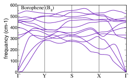
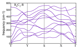
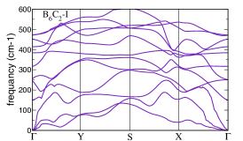
Due to high flexibility, the range of strain at which borophene remains stable is very much higher than that of other 2D materials such as silicene Roman , MoS2 Wang and black phosphorene Li , and yet, slightly larger than graphene Liu and h-BN Wu . We expect it can also be able to withstand strong strain generated by carbon substitutions. Nevertheless, we need to confirm whether the borophene remains stable by the chemical substitutions with C atoms. Study of phonon dispersion provides a way to investigate the dynamical stability of crystal structures. The calculated phonon dispersions of pure borophene and two systems in which a dimer of C atoms is substituted into borophene (B6C2-R-[C5C6] and B6C2-I-[C2C3]) are shown in Fig. S8. In this method, the negative value of imaginary phonon frequencies is an indication of dynamical instability. As can be seen in Fig. S8, there are no negative imaginary frequencies, and therefore all three systems studies here are stable with respect to substitution of C atoms for B atoms.
VIII Ab initio hopping matrices elements
The parameters of our coarse-grained structure are obtained from atomic scale hopping parameters depicted in panel (a) of Fig. S3. Based on these parameters, as explained in section VI, the effective hopping parameters of our effective model defined on the parent honeycomb structure are calculated. The accurate determination of the effective parameters therefore depends on accurate ab initio calculation of atomic hoppping amplitudes that can be extracted from the corresponding Wannier functions Mostofi ; Freimuth ; Marzari .
The honeycomb lattice tight-binding model presented in our paper to describe the formation of tilt in structure is rather generic, and the hopping parameters can span a wide range of values. Nevertheless for a specific material they are fixed numbers. In contrast to graphene where hopping energy to sites further away than nearest neighbours are much smaller than the first neighbor hopping, our renormalized hopping scenario predict large effective hopping mediated by BR atoms in borophene. Even the graphene fits within our renormalized hopping picture, as in the case of pure graphene, there are no ridge sites, and hence all parameters other than the nearest neighbor hoppings are nearly zero. In contrast, in the structure, they are numerically on the scale of electron volts, giving rise to effective hopping parameters of the same order. So it is sufficient to calculate the atomic parameters.
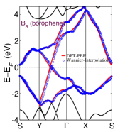
We calculate the hopping energies for all considered systems using Wannier functions. The maximally localized Wannier functions (MLWFs) are constructed with the WANNIER90 library Mostofi ; Freimuth . It is worth noting that graphene show well-isolated bands at the Fermi energy, which induces a simple single band model with states. In borophene, our projected band-structure indicate that the states of BR atoms are not completely isolated from the states. To verify the adequacy of the above orbitals and hence the validity of calculated Wannier functions, in Fig. S9 for three B8, B6C2-R-[C5C6], and B6C2-I-[C2C3] systems, we compare the DFT-PBE band structure (solid red) with the corresponding Wannier-interpolated bands (blue) obtained with Wannier orbitals on the BI site and the and Wannier orbitals on the BR-site. To avoid complexity, only four bands with character are shown. As seen from the band structures, the overall agreement between original and Wannier-interpolated bands is remarkably good. Small deviations appear for states far from the Fermi energy, which given our picture based on the renormalization, are irrelevant for the low-energy physics.
Now that we have established in Fig. S9 that the orbitals of inner sites and and orbitals of ridge sites are relevant degrees of freedom, we are ready to calculate the parameters by inclusion of these orbitals. The results of ab initio hopping matrix elements for pure borophene, B7C1-I-[C2], B7C1-R-[C5], B6C2-R-[C5C6], and B6C2-I-[C2C3] are presented in the left partition of Table 4. These values are then used to derive the parameters of the effective model in the right partition of the same table. When a dimer of BR atoms occupying the ridge sites is replaced by a C dimer B6C2-R-[C5C6], we obtain comparatively large matrix elements (except ). This is due to the fact that the ridge atoms come closer to the plane upon replacement by C atoms as depicted in Fig. 5(a) of main text. So, the ridge atoms mediate stronger hoppings in B6C2-R-[C5C6] system, meaning that they can better connect further away inner sites on the effective honeycomb model. As a consequence, the tilt of Dirac-cone is considerably larger than the corresponding values in pristine borophene. The situation is reversed when BI atoms of the inner sites are replaced by a dimer of C atoms B6C2-I-[C2C3]. In this case, the ridge atoms move away from the plane of inner atoms, as a results, the hopping parameters are smaller than corresponding ones in pristine borophene. In this situation, the system tends to reduce the tilt of Dirac cone.
| system | |||||||||||||||
|---|---|---|---|---|---|---|---|---|---|---|---|---|---|---|---|
| pure borophene | 2.09 | -2.66 | 2.09 | 2.09 | -1.87 | -1.87 | -1.87 | -2.54 | -2.21 | -2.36 | -1.07 | -1.99 | -2.51 | 0.46 | 0.48 |
| B7C1-I-[C2] | 2.21 | -2.59 | 2.32 | 2.35 | -1.52 | -1.61 | -1.47 | -2.35 | -2.32 | -1.87 | -1.19 | -1.88 | -2.40 | —- | —- |
| B7C1-R-[C5] | 2.23 | -2.73 | 2.25 | 2.14 | -1.89 | -1.74 | -1.85 | -2.13 | -2.30 | -2.03 | -1.09 | -2.11 | -2.69 | 0.56 | 0.42 |
| B6C2-I-[C2C3] | 1.93 | -2.52 | 1.96 | 1.92 | -1.52 | -1.52 | -1.55 | -2.34 | -2.37 | -1.75 | -0.95 | -1.62 | -2.05 | 0.36 | 0.66 |
| B6C2-R-[C5C6] | 2.14 | -2.33 | 2.12 | 2.15 | -2.23 | -2.21 | -2.20 | -2.43 | -2.05 | -2.49 | -1.09 | -2.24 | -2.85 | 0.59 | 0.32 |
Now that we have a picture of the formation of the Dirac cone, and an analytical model to produce it, we use the model parameters obtained in Table 4 to construct a picture of tilted Dirac cone as a function of in pure and C-doped borophene. The solution of the tight-binding model leads to the , where the further neighbor effective hoppings and of the model are calculate in the right partition of Tab. 4. As shown in Table. 4, placing C atoms in the ridge sites generates larger that ultimately increases the tilt from the of the pristine borophene to in B6C2-R-[C5C6]. Employing Eqs. (S13) and (S14) the energy dispersion for pristine borophene, B6C2-I-[C2C3], and B6C2-R-[C5C6] are reconstructed in Fig. S10 using the ab initio effective hopping amplitude reported in Tab. 4.

Accuracy of tilt parameters: The ultimate outcome of our model is to understand the mechanism of the formation of the tilt. Hence the value of tilt parameters are important. Let us close this supplementary material by a comparison between the values of the tilt parameter directly extracted from the ab initio data, and the tilt parameter predicted by Eq. (S15) of our model.
We extract the tilt directly from the DFT data by fitting the slopes and of the ab initio dispersion relations along the direction as,
Using the direct DFT data, we find that the tilting parameter value are , , and in pristine borophene, B6C2-I, and B6C2-R-[C5C6] respectively. This is in qualitative agreement with the values obtained from our model, Eq. (S15) and the trend in tilt values upon placing the carbon atoms in ridge/inner sites are correctly reproduced in our model (see Tab. 4). The physical picture emerging from both DFT data and our model is that the substitutions of BR atoms by C dimers where the two C atoms belong to the ridge sites can increase the tilt of Dirac cone. Moreover, the location of tilted Dirac-cone is very sensitive to the position of C atoms on the lattice. This location has been quantified by the parameter to measure the distance from Dirac point to and the results are reported in Tab. 4. If C atoms are replaced in the ridge sites, Dirac-node moves closer to point.
To conclude, the tilted Dirac cone dispersion in borophene can be well described by our effective tight-binding model. This effective model is not only important for understanding the origin of formation of the tilt in the Dirac cone in borophene, but it also increases considerably the predictive power to find new compounds possessing tilted Dirac cone. Furthermore, out concrete model paves the path for many other studies including the effects of interactions/disorder/symmetry breaking, etc in a physically motivated model of tilted Dirac cone in space group.
References
- (1) C. Kittel, Quantum Theory of Solids, 2nd revised ed. (John Wiley and Sons, New Jersey, 1983).
- (2) G. D. Mahan, Applied Mathematics (Springer, Boston, MA, 2002).
- (3) X. Fan, D. Ma, B. Fu, C.-C. Liu, and Y. Yao, Physical Review B 98, 195437 (2018).
- (4) M. S. Dresselhaus, G. Dresselhaus, and A. Jorio, Group Theory: Application to the Physics of Condensed Matter (Springer Science and Business Media, Berlin, Heidelberg, Germany, 2007).
- (5) C. Bradley and A. Cracknell, The Mathematical Theory of Symmetry in Solids: Representation Theory for Point Groups and Space Groups (Oxford University Press, Oxford, England, UK, 2010).
- (6) Barry Bradlyn, L. Elcoro, M. G. Vergniory, Jennifer Cano, Zhijun Wang, C. Felser, M. I. Aroyo, and B. Andrei Bernevig, Phys. Rev. B 97, 035138 (2018).
- (7) B. Bradlyn, L. Elcoro, J. Cano, M. Vergniory, Z. Wang, C. Felser, M. Aroyo, and B. A. Bernevig, Nature 547, 298 (2017).
- (8) https://www.cryst.ehu.es/
- (9) https://www.quantum-espresso.org
- (10) J. P. Perdew, K. Burke, and M. Ernzerhof, Phys. Rev. Lett. 77, 3865 (1996).
- (11) F. Liu, P. Ming, J. Li, Phys. Rev. B 2007, 76, 064120.
- (12) J. Wu, B. Wang, Y. Wei, R. Yang, M. Dresselhaus, Mater. Res. Lett. 2013, 1, 200.
- (13) T. Li, Phys. Rev. B 2012, 85, 235407.
- (14) R. E. Roman, S. W. Cranford, Comput. Mater. Sci. 2014, 82, 50.
- (15) L. Wang, A. Kutana, X. Zou, B. I. Yakobson, Nanoscale 2015, 7, 9746.
- (16) A. A. Mostofi, J. R. Yates, Y.-S. Lee, I. Souza, D. Vanderbilt, and N. Marzari, Comput. Phys. Commun. 178, 685 (2008).
- (17) F. Freimuth, Y. Mokrousov, D.Wortmann, S. Heinze, and S. Blügel, Phys. Rev. B 78, 035120 (2008).
- (18) N. Marzari and D. Vanderbilt, Phys. Rev. B 56, 12847 (1997).
- (19) T. Farajollahpour, Z. Faraei, S. A. Jafari, Phys. Rev. B 99 235150 (2019)