Thermal radio absorption as a tracer of the interaction of SNRs with their environments

We present new images and continuum spectral analysis for 14 resolved Galactic SNRs selected from the 74 MHz Very Large Array Low-Frequency Sky Survey Redux (VLSSr). We combine new integrated measurements from the VLSSr with, when available, flux densities extracted from the Galactic and Extragalactic All-Sky Murchison Widefield Array Survey (GLEAM) and measurements from the literature to generate improved integrated continuum spectra sampled from $\sim$15 MHz to $\sim$217 GHz. We present the VLSSr images. When possible we combine them with publicly available images at 1.4 GHz, to analyse the resolved morphology and spectral index distribution across each SNR. We interpret the results and look for evidence of thermal absorption caused by ionised gas either proximate to the SNR itself, or along its line of sight. Three of the SNRs, G4.5+6.8 (Kepler), G28.6$-$0.1, and G120.1+1.4 (Tycho), have integrated spectra which can be adequately fit with simple power laws. The resolved spectral index map for Tycho confirms internal absorption which was previously detected by the Low Frequency Array (LOFAR: Arias et al. 2019b), but it is insufficient to affect the fit to the integrated spectrum. Two of the SNRs are pulsar wind nebulae, G21.5$-$0.9 and G130.7+3.1 (3C 58). For those we identify high-frequency spectral breaks at 38 and 12 GHz, respectively. For the integrated spectra of the remaining nine SNRs, a low frequency spectral turnover is necessary to adequately fit the data. In all cases we are able to explain the turnover by extrinsic thermal absorption. For G18.8+0.3 (Kes 67), G21.8$-$0.6 (Kes 69), G29.7$-$0.3 (Kes 75), and G41.1$-$0.3 (3C 397), we attribute the absorption to ionised gas along the line of sight, possibly from extended HII region envelopes (EHEs). For G23.3$-$0.3 (W41) the absorption can be attributed to HII regions located in its immediate proximity. Thermal absorption from interactions at the ionised interface between SNR forward shocks and the surrounding medium were previously identified by Brogan et al. (2005) as responsible for the low frequency turnover in SNR G31.9+0.0 (3C 391); our integrated spectrum is consistent with the previous results. We present evidence for the same phenomenon in three additional SNRs G27.4+0.0 (Kes 73), G39.2$-$0.3 (3C 396), and G43.3$-$0.2 (W49B), and derive constraints on the physical properties of the interaction. This result indicates that interactions between SNRs and their environs should be readily detectable through thermal absorption by future low frequency observations of SNRs with improved sensitivity and resolution.

1 Introduction

Supernova remnants (SNRs) are the most prominent extended sources of non-thermal emission in the Galaxy and impact Galactic astrophysics in several important ways. They and their supernovae (SNe) progenitors play a key role in stellar evolution by marking the death of massive stars, redistributing the atomic elements produced within them, and stimulating the birth of new stars through their interaction with molecular clouds. SNR shocks significantly impact the dynamics and evolution of the interstellar medium (ISM) (Breitschwerdt et al., 2017), and play a major role in shaping its long lived structure (McKee & Ostriker, 1977). As the presumed primary acceleration sites for Galactic cosmic rays (CRs) through diffusive shock acceleration (Caprioli, 2010; Gabici et al., 2019; Kachelrieß & Semikoz, 2019), they seed the ISM with at least $\sim$1/3 of its energy density. A complete census of Galactic SNRs, an elusive goal long prevented by observational selection effects (Green, 1991), would offer powerful constraints on the Galactic SNe rate.

At radio wavelengths, SNRs are spatially extended and typically prolific non-thermal emitters over a broad range of frequencies. Accurate radio spectra for SNRs can be used to trace interactions with the ISM, and to test predictions from diffusive shock acceleration and SNR evolution theories. For largely technical reasons (Kassim et al. 2007, and references therein), low frequency ($\nu<100$ MHz) radio observations of SNRs have historically been limited by extremely poor angular resolution and sensitivity, typically an order of magnitude or more worse than what is achieved at higher (GHz) frequencies. The scientific impact for SNRs has been significant, limiting a number of unique and important studies that critically rely on precise low frequency measurements. These include: (i)  Deviations from power law spectra for SNRs predicted by theory, which can only be constrained by measurements encompassing a very large range of frequencies (Reynolds & Ellison 1992). Because the deviations are subtle, a high degree of accuracy is needed. For most SNRs these have been unavailable until only recently (Urošević, 2014; Arias et al., 2019a). (ii)  Thermal absorption in and around SNRs, which is uniquely measured at low frequencies ($\nu<100$ MHz). It may arise intrinsically, indicating the presence of thermal material interior to the SNR, e.g. unshocked ejecta, or extrinsically from the interaction of the SNR with its immediate surroundings. Due to limited observational capabilities, intrinsic thermal absorption has only been detected in the brightest SNRs, including the Crab nebula (Bietenholz et al., 1997), Cas A (Kassim et al., 1995; DeLaney et al., 2014; Arias et al., 2018), and Tycho (Arias et al., 2019b). External thermal absorption is a tracer of the ionised interface generated as an SNR interacts with its immediate surrounding in Galactic complexes. In addition to probing this interaction, it provides constraints on the relative radial superposition of thermal and non-thermal constituents in complex regions (Brogan et al., 2003, 2005). (iii)  The distribution of ionised gas in the ISM unrelated to SNRs, which can be measured using SNRs as background beacons (Kassim, 1989b). (iv)  The Galactic SNe rate, which is poorly known due to incompleteness in Galactic SNR catalogues. Low frequency observations of SNRs are a proven means of addressing the incompleteness (Brogan et al., 2004, 2006; Hurley-Walker et al., 2019).

Starting in the 1990s (Kassim et al., 1993), technical breakthroughs enabled a succession of dramatic improvements in low radio frequency observational capabilities (van Haarlem et al., 2013). The scientific impacts have so far mainly been realised for extragalactic studies (e.g. van Weeren et al. 2016; Shimwell et al. 2017), but the impact on Galactic SNRs studies is slowly starting to be felt (e.g. Brogan et al. 2006; Supan et al. 2018; Arias et al. 2018). The 74 MHz Very Large Array Low-frequency Sky Survey Redux (VLSSr) was the first all-sky survey to take advantage of the improved low frequency capability (Lane et al., 2014). As such the VLSSr established an important calibration grid for a suite of emerging new instruments. While technically limited compared to a rapidly advancing state of the art, it also remains an important resource for individual source studies. In particular, its potential for SNR studies has remained largely untapped. In this paper we present a sample of 14 bright, resolved SNRs selected from the VLSSr, which we use to address a number of the scientific issues outlined above, and to stimulate future studies as larger samples of weaker sources become accessible with modern instruments, e.g. the LBA Sky Survey (LoLSS: de Gasperin et al. 2021) with LOFAR.

This paper is organised as follows. In Sect. 2 we describe our selection of the 14 bright Galactic SNRs from the VLSSr images analysed in this paper. We measure their integrated 74 MHz flux densities. When available, we also measure their low frequency flux densities from the Galactic and Extragalactic All-sky Murchison Widefield Array Survey (GLEAM, Wayth et al. 2015; Hurley-Walker et al. 2019). The method used to construct spectral index maps is explained in Sect. 3. In Sect. 4.1 we assimilate the new low radio frequency fluxes into a larger framework of measurements from the literature, and use it to construct improved integrated continuum spectra. Careful attention is given to anchoring these spectra on an accurate, absolute flux density scale which is valid over most of the frequency range considered for each source (Perley & Butler, 2017). Together with the inclusion of new low frequency measurements the derived spectra are a marked improvement over previous studies, as explained in Sect. 4.2. In Sect. 5 we discuss the spatially resolved morphology and spectral index behaviour for each individual SNR. In Sect. 6 we focus on those sources whose spectral analysis presents deviations from a canonical power law at the lowest frequencies, attributable to thermal absorption. We analyse the properties of the surrounding medium in order to understand the physical context of the absorption, i.e. whether it is intrinsic, extrinsic and proximate to the SNR, or attributable to more distant ISM from along the line of sight. We present our summary and conclusions in Sect. 7.

2 General Properties of the VLSSr SNR sample

Based on their radio morphologies, our sample comprises 10 shell-type, 2 composite, and 2 plerion SNRs, all of which are previously known (Green, 2019). Three of the SNRs in the list are also part of the mixed-morphology (MM) class showing centrally condensed thermal X-ray emission surrounded by a synchrotron radio shell. Twelve sources analysed in this work belong to the first Galactic quadrant from $l\sim$+4^∘ to $l\sim$+44^∘, while the remaining two objects are located in the second quadrant, in the 120^∘ $\leq$ $l$ $\leq$131^∘ region. All of them are located within Galactic latitudes $-$1^∘ $\leq$ $b$ $\leq$7^∘.

2.1 VLSSr Data

In Fig 1, we present images for each of the 14 SNRs from the VLSSr. The observations are centred at a frequency of $\nu=74$ MHz with an angular resolution of $\theta\sim 75^{\prime\prime}$. The images are sensitive to spatial structures up to $\sim$36^′ in size, larger than the full extent of any SNR in our sample. In all cases the emission is displayed above a 4-$\sigma$ noise level measured in the corresponding VLSSr fields (the mean rms noise level of the maps is $\sim$0.16 Jy beam^-1). For the majority of the SNRs in our sample, the VLSSr maps represent the most complete available image of the source, both resolving the structure and recovering the diffuse emission in the low frequency regime below 100 MHz (see, for instance, Slee, 1977; Kassim, 1988). The morphological properties of each SNR at 74 MHz are discussed below in Sect. 5. Throughout this paper each SNR is referred to by the name most commonly used in the literature. The correspondence with the name derived from the Galactic coordinates of the centre of the source is indicated in Table 1.

As a qualitative measure of the consistency of our source size measurements at 74 MHz, we compared them to their counterparts at 1.4 GHz taken, depending on the sky position, from the Multi-Array Galactic Plane Imaging Survey (MAGPIS, Helfand et al. 2006) or the NRAO VLA Sky Survey (NVSS, Condon et al. 1998). We constrained our measurements to regions exceeding at least 3 times the respective rms noise levels in the images at 74 MHz and 1.4 GHz. In all cases the 1.4 GHz images were convolved to the VLSSr resolution (75^′′). In general the source sizes are expected to match with a few exceptions. The source could appear larger at 74 MHz than at 1.4 GHz if the higher frequency observations miss faint, extended structure (see for example, Lane et al., 2004). Alternately, foreground thermal absorption along the line of sight can unevenly attenuate the synchrotron emission across the SNR and cause the source to appear smaller at 74 MHz (Lacey et al., 2001). Finally, residual ionospheric calibration errors can distort the apparent source size at 74 MHz (a further discussion of this non-physical effect is presented in Cohen et al., 2007).

Despite these unknowns, our comparison indicated a remarkably good agreement in source size for 11 of our sources, with 74 MHz/1.4 GHz-size ratios $\sim 1.04$. Two sources, W41 and 3C 391, have ratios of $\sim 0.26$ and $\sim 0.87$, respectively, indicating they are substantially smaller at 74 MHz than at 1.4 GHz. W41 sits inside the giant molecular complex G23.3$-$0.4, and is spatially coincident with several HII regions (Messineo et al. 2014, Hogge et al. 2019). As discussed in Sect. 6.3.1, we attribute the reduced apparent size at 74 MHz to absorption by HII regions in the complex blocking the SNR emission. For SNR 3C 391 the result is consistent with data presented in Brogan et al. (2005), who attributed it to thermal absorption tracing the ionised interface along the SNR/molecular cloud interface. SNR 3C 396, on the other hand, has a ratio of $\sim 1.4$, indicating it is significantly more extended at 74 MHz than at 1.4 GHz. We attribute this to the higher frequency measurements missing the very faint emission at the northwest edge. With these three exceptions accounted for, we feel confident that our VLSSr measurements provide a robust sampling of the full SNR source sizes at 74 MHz.

Basic radio source parameters were measured from the VLSSr images, such as the angular dimensions, the total and peak flux density, and the surface brightness of each SNR in the sample. All of them are reported in Table 1. For each SNR the integrated flux density was derived by using a polygonal region to fit the outer radio boundary of the remnant 4 $\sigma$ above the intrinsic noise level measured in the corresponding VLSSr field. When necessary, depending on the fluctuations of the background emission around the source, the flux density estimate was corrected for an average background level. This contribution was determined by scanning in both right ascension and declination through several positions surrounding the SNR. The main errors in the listed flux densities arise from intensity-proportional flux-density uncertainties in both the absolute flux-density scale ($\sim$15%) and primary beam corrections, as well as uncertainties in the background estimations and bias corrections. All of these contributions were combined in quadrature to compute the final error in the integrated flux density measurements. Surface brightness estimates at 74 MHz were calculated from the relation $\Sigma_{74}=1.505\times 10^{-19}\,S_{74}/A_{74}$ W m^-2 Hz^-1, where $S_{74}$ is the integrated flux density (in Jy) measured in the VLSSr map and $A_{74}$ represents the area (in square arc minutes) enclosed by the polygon region used to integrate the 74 MHz emission. The mean percentage error in our surface brightness estimates is $\sim$30% and is dominated by uncertainties in defining the outer boundary of the radio emission. The flux density measurements from the VLSSr maps analysed here add to the scarce list of reliable low-frequency estimates available to date.

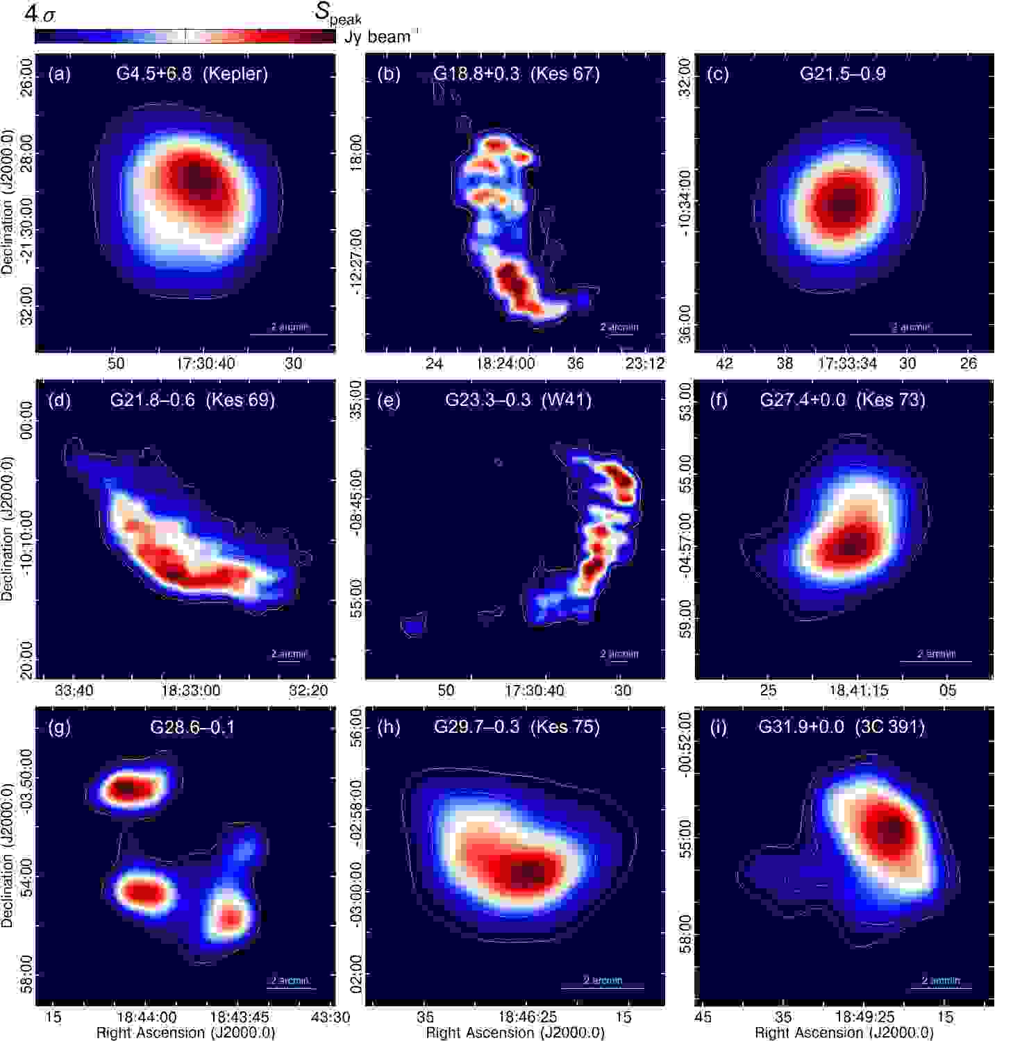
Figure 1: The VLSSr 74 MHz images for the 14 SNRs in our sample, with an 75^′′ angular resolution. The colour scale, given on top, is linear scaling from 4 times the local rms noise level (4 $\sigma$) to the peak intensity value of the subimage, $S_{\mathrm{peak}}$ (see values quoted in Table 1). The contours levels of the 74 MHz emission start at 4 $\sigma$ increasing in steps of 25, 50, and 75% of the scale range. Exceptions are Tycho and 3C 397 for which an 8-$\sigma$ lower limit was chosen. A cyan horizontal line of 2^′ length is included in each panel to facilitate the comparison between the SNRs’ sizes.

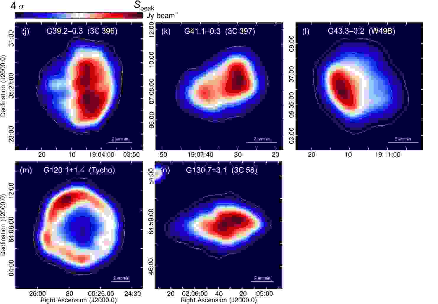
Figure 1: Continued.

Table 1: Continuum properties for all the SNRs in our sample derived from the 74 MHz VLSSr images.

Galactic	Alternative	Morphological	Size	VLSSr Flux	$\Sigma_{74}$	VLSSr rms	$S_{\mathrm{peak}}$
name	name	Class	$\theta_{\mathrm{max}}$[′] $\times$ $\theta_{\mathrm{min}}$[′]	Density[Jy]	[W m-2 Hz-1 sr-1]	[Jy beam-1]	[Jy beam-1]
G4.5$+$6.8	Kepler	Shell	$5\times 5$	$111\pm 17$	$6.7\times 10^{-19}$	0.23	24.4
G18.8$+$0.3	Kes~67	Shell	$17\times 11$	$76.2\pm 13.8$	$6.1\times 10^{-20}$	0.14	1.9
G21.5$-$0.9	–	Plerion	$3.2\times 3.2$	$6.4\pm 1.1$	$9.4\times 10^{-20}$	0.15	4.1
G21.8$-$0.6	Kes~69	Shell	$22\times 10$	$169\pm 31$	$1.2\times 10^{-19}$	0.18	4.5
G23.3$-$0.3	W41	Shell	$18\times 7$	$88\pm 17$	$1.1\times 10^{-19}$	0.14	2.3
G27.4$+$0.0	Kes~73	Shell	$6\times 5$	$13.8\pm 2.5$	$6.9\times 10^{-20}$	0.14	2.8
G28.6$-$0.1	–	Shell	$9.5\times 7.0$	$26.9\pm 4.7$	$6.4\times 10^{-20}$	0.15	2.4
G29.7$-$0.3	Kes~75	Composite	$4.5\times 3.5$	$48.5\pm 7.9$	$4.6\times 10^{-19}$	0.22	14.0
G31.9$+$0.0	3C~391	MM	$6.5\times 5.5$	$31.5\pm 5.4$	$1.2\times 10^{-19}$	0.20	4.9
G39.2$-$0.3	3C~396	Composite	$7.5\times 7.5$	$44.8\pm 8.8$	$1.2\times 10^{-19}$	0.16	4.0
G41.1$-$0.3	3C~397	MM	$5.5\times 4.0$	$68.9\pm 10.6$	$4.7\times 10^{-19}$	0.16	12.7
G43.3$-$0.2	W49B	MM	$5.5\times 5.5$	$64.0\pm 10.1$	$3.2\times 10^{-19}$	0.13	11.6
G120.1$+$1.4	Tycho	Shell	$9\times 9$	$255.0\pm 38.8$	$4.7\times 10^{-19}$	0.15	14.5
G130.7$+$3.1	3C~58	Plerion	$8.5\times 4.5$	$34.6\pm 5.3$	$1.4\times 10^{-19}$	0.08	3.7

2.2 GLEAM

In order to more fully probe the low frequency spectra of the SNRs, we also looked at recently published images from GLEAM. This survey currently covers parts of the Galactic Plane at frequencies of 88, 118, 155, and 200 MHz, at resolutions from $4^{\prime}-2^{\prime}$ (Hurley-Walker et al., 2019). For 12 of the 14 SNRs we were able to obtain flux density measurements from GLEAM published images, and we report these measurements in Table 2. At the time we made the analysis, there were no images available for the remaining two remnants. In some cases the images were of lower quality, and we chose not to use them for this study. We measured the fluxes and errors using the same method described above for the VLSSr images. Because the images are at a lower resolution which does not resolve many of the remnants, we present only the integrated flux measurements in this work.

Table 2: Integrated flux densities measured from GLEAM Survey images of 12 SNRs in our study.

Source (alias)	Flux density [Jy]
	88 MHz	118 MHz	155 MHz	200 MHz
G4.5$+$6.8  (Kepler)	$100\pm 9$	$77\pm 7$	$62\pm 9$	…
G18.8$+$0.3  (Kes 67)	$81\pm 17$	$80\pm 14$	$71\pm 11$	$62\pm 9$
G21.5$-$0.9	$7.2\pm 2.7$	$6.6\pm 2.0$	$6.3\pm 1.3$	$5.9\pm 1.1$
G21.8$-$0.6  (Kes 69)	$194\pm 21$	$166\pm 20$	$143\pm 16$	$116\pm 14$
G23.3$-$0.3  (W41)	$154\pm 30$	$172\pm 40$	$149\pm 37$	$139\pm 28$
G27.4$+$0.0  (Kes 73)	$17.0\pm 3.5$	$17.6\pm 2.9$	$14.6\pm 3.0$	…
G28.6$-$0.1	$29.5\pm 5.6$	$25.9\pm 3.9$	$20.2\pm 3.1$	$15.5\pm 1.9$
G29.7$-$0.3  (Kes 75)	…	$42.3\pm 5.8$	$32.4\pm 3.4$	$25.5\pm 2.7$
G31.9$+$0.0  (3C 391)	$43.7\pm 8.0$	$48.1\pm 4.9$	$44.4\pm 4.1$	…
G39.2$-$0.3  (3C 396)	…	$39.9\pm 4.9$	$33.9\pm 3.4$	$28.5\pm 2.8$
G41.1$-$0.3  (3C 397)	$57\pm 7$	…	…	…
G43.3$-$0.2  (W49B)	$63.8\pm 8.0$	$69.7\pm 5.5$	…	…

3 Local SNR variations in the radio spectral index

Local changes in the radio spectral index across each source were computed for our targets by combining the VLSSr maps with the best available image of the source from surveys at 1.4 GHz (e.g., MAGPIS, NVSS, VLA Galactic Plane Survey (VGPS, Stil et al. 2006), and the NRAO VLA Archive Survey (NVAS)). Since we do not have the uv-data for the higher frequency images, we created the spectral index maps in a standard way from the direct ratio of the images at both frequencies. While doing this, we aligned, interpolated, and smoothed the 1.4 GHz maps to matching VLSSr ones. Additionally, only regions with flux densities greater than 4-$\sigma$ significance level of their respective sensitivities were used in the process. The resulting spectral index images are displayed in Fig. 2. Errors on these maps are of order $\sim$20-25% for the local spectral index measurements. We are aware that a quantitative interpretation of spectral variations with position is not possible from the resulting maps, but they are very useful to reveal qualitative trends. The analysis of the radio spectral index images is presented in Sect. 5. We note that for SNR 3C 397 (G41.1$-$0.3) the public radio continuum images at radio frequencies higher than 74 MHz do not recover the expected flux density accurately, and thus we decided not to create a spectral index map for this source.

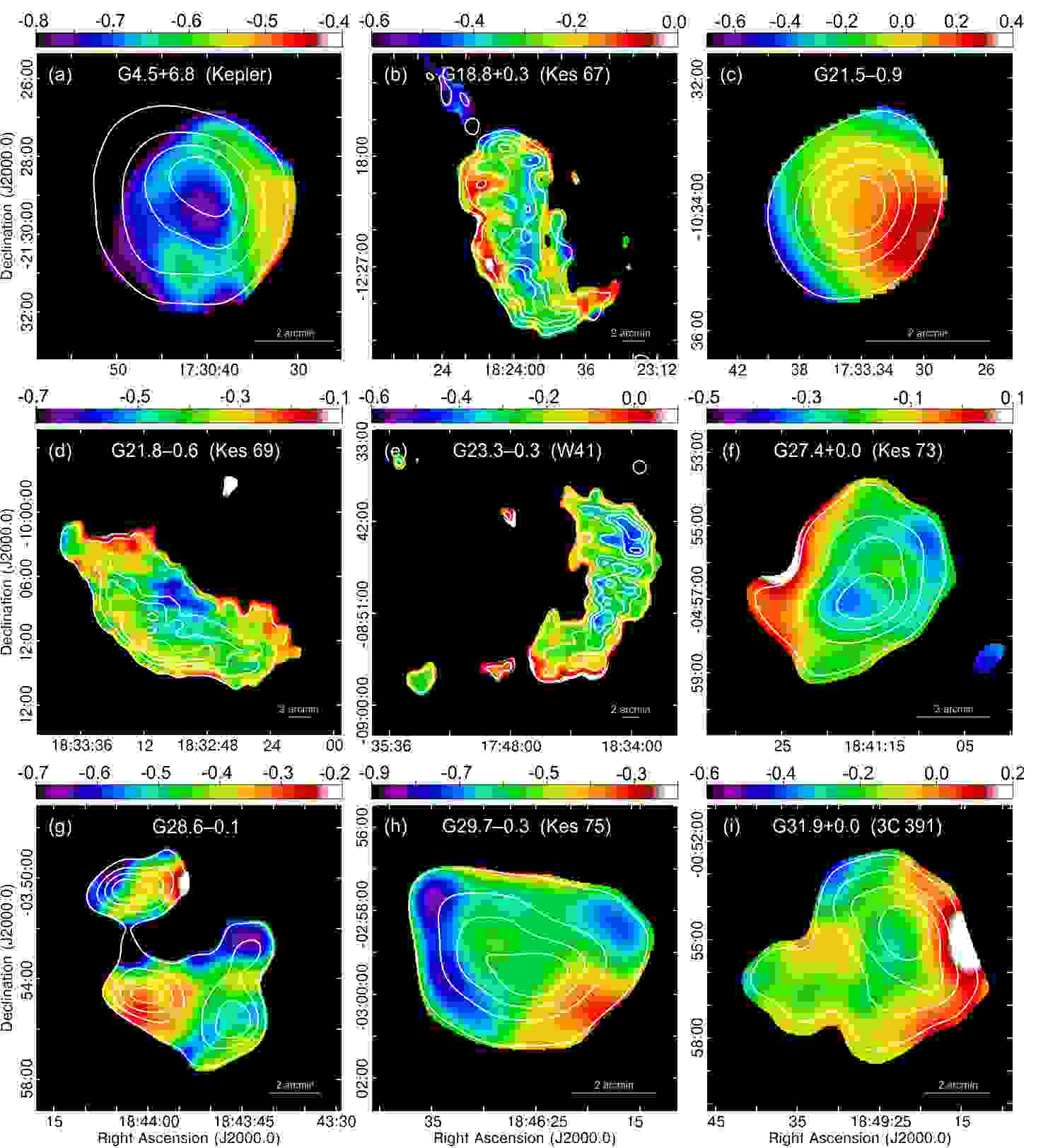
Figure 2: Spectral index maps between 74 MHz and 1.4 GHz (resolution 75^′′) for the SNRs in our sample (except the source 3C 397). The maps were constructed by combining the VLSSr image with those available from radio continuum surveys (see text for details). Pixels with brightness below 4$\sigma$ at 74 MHz or 1.4 GHz were blanked. The colour scales displayed at the top of the maps indicate the spectral indices measured over each SNRs. The radio continuum emission from VLSSr 74 MHz at a resolution of 75^′′ is represented by contours. For reference, we used the same contours levels as in Fig. 1.

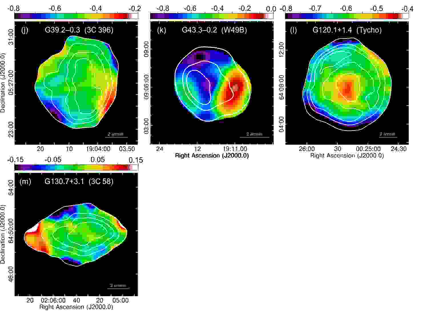
Figure 2: Continued

4 Integrated SNR radio continuum spectra

4.1 Newly derived integrated spectra

The global spectral properties of SNRs have been determined in a number of previous studies. However, the majority of them were based on the combination of data without using a common radio flux density scale, thereby making the quantitative comparison of measurements incorrect. In a few cases, the absolute scale of Baars et al. (1977) was used, although it was applied even at frequencies lower than 300 MHz or higher than 15 GHz for which the scale is incomplete. In addition, published spectra include observations with low angular resolution and surface brightness sensitivity, which in complex regions of the Galaxy can easily miss non-thermal components in the emission by confusion with Galactic background or thermal sources. The inclusion in the collected data of widely scattered flux density measurements at similar frequencies as well as differences in the quality of the data not correctly weighted in the analysis, also affect the reliability of previously published spectra.

Flux densities included in our 14 integrated spectra were selected based on the following criteria: i) we only included measurements with error estimates less than 30%, ii) measurements with deviations well beyond the best-fit model and inconsistent with the reported errors were excluded, iii) at frequencies above 1 GHz, we excluded interferometer measurements with insufficient short spacings to sample the extended source flux, and iv) we excluded single-dish measurements with poor resolution that may overestimate flux densities due to high confusion levels. Based on these criteria we compiled 454 flux density measurements across the frequency range of 15 MHz - 217 GHz. We combine these with the newly measured VLSSr and GLEAM flux densities to create updated integrated radio spectra for the SNRs in our sample. The VLSSr and GLEAM points help fill in the low frequency portion of the spectra most poorly constrained by past measurements from Culgoora (80 MHz, Slee 1977), Clark Lake TPT (30.9 MHz, Kassim 1988), and the Pushchino telescopes (83 MHz, Kovalenko et al. 1994a).

When possible, the measurements were adjusted to the absolute flux density scale provided by Perley & Butler (2017). This scale, established between 50 MHz and 50 GHz, is accurate to 3% and up to 5% for measurements at the extreme of the frequency range. For $\sim 20\%$ of the literature fluxes, correction was not possible because of insufficient information on primary flux calibration in the original reference, or because the frequency was outside the range for which the flux scale is defined. For these sources we included the values as reported without adjustment. The final set of flux densities used to construct the integrated spectra are presented in Appendix A.

In Fig. 3 we present the radio continuum spectra for all SNRs in our study. VLSSr and GLEAM flux densities are indicated by filled red and yellow symbols, respectively, and all points are weighted by their estimated uncertainties. In each spectrum the 1- and 2-$\sigma$ error in the best-fit values is represented by gray-shaded regions. We found that 5 of the SNRs could be fit by power law functions defined by the relation $S_{\nu}\propto\nu^{\alpha}$, in which $S_{\nu}$ denotes the flux density at the frequency $\nu$. This includes the two pulsar wind nebulae (PWNe) in our sample, whose spectra were fit by broken power laws. The remaining cases show evidence of absorption below 100 MHz (Kassim, 1989a), and we fit the spectra with a power law and an exponential turnover, according to Eq. 1,

$$S_{\nu}=S_{\nu_{0}}\,\left(\frac{\nu}{\nu_{0}}\right)^{\alpha}\,\mathrm{exp}\left[-\tau_{\nu_{0}}\,\left(\frac{\nu}{\nu_{0}}\right)^{-2.1}\right].$$ (1)

where $\nu_{0}$ is the reference frequency, set to 74 MHz, at which the integrated flux density $S_{\nu_{0}}$ and optical depth $\tau_{\nu_{0}}$ are measured.

This is a simplistic fitting model, and we note that there are theoretical grounds to expect intrinsically curved SNR spectra, both spatially resolved and integrated. Concave-up curvature has been linked to non-linear acceleration processes in young SNRs (e.g. Tycho, Kepler; Reynolds & Ellison 1992) (see also Sect. 5). Conversely, concave-down spectra have been linked to bends in the energy distribution of the radiating electrons (Anderson & Rudnick, 1993). Also, synchrotron losses, thermal bremsstrahlung, and spinning dust in evolved SNRs (e.g. 3C 391 and 3C 396) interacting with high density environments have been proposed to flatten spectra at higher frequencies ($\sim$10-100 GHz) (Urošević, 2014). Since we find no compelling evidence for these signatures in our spectra, we proceeded with the power law plus thermal absorption model. There is still tremendous room for significantly improved measurements, at both high and low frequencies, that may well eventually justify more complex modelling for many of these sources.

Table 3 provides a summary of the best-fit spectral indices and free-free optical depths (when appropriate) from the weighted fit to the integrated continuum spectra shown in Fig. 3. We also include any values for these parameters previously published in the literature. The new results are used in Sect. 6 to constrain the physical properties (electron measure, $\mathrm{EM}$, and electron density, $n_{\mathrm{e}}$) of the foreground ionised gas responsible for the measured spectral turnovers.

In Fig. 4a we have plotted the distribution of the integrated radio spectral indices from our power-law fits. For comparison, the age and morphology of each source is also indicated in Fig. 4b. For our purpose, we adopted the usual classification of “young” to refer to a SNR in either the free-expansion or the early Sedov phase of its evolution ($\lesssim$3000 yr). SNRs in subsequent evolutionary stages are considered evolved, an admitted simplification as multiple evolutionary phases may occur simultaneously in different parts of a SNR. We found that 8 sources have relatively steep spectra ($|\alpha|>0.5$), 5 of which are young. In addition, there are 4 SNRs with flatter radio spectra ($|\alpha|<0.5$). The remaining two sources are the pulsar wind nebulae G21.5$-$0.9 and 3C 58, for which the continual injection of energetic electrons produces even flatter integrated spectra. These results are further discussed in Sect. 5.

The spectral indices that we have measured in this work for young and evolved SNRs disagree with test particle predictions from diffusive shock acceleration theory (Reynolds et al., 2012; Urošević, 2014). In the linear regime, flatter spectral indices (the flattest possible value is $\alpha=-0.5$) are predicted for parallel shocks in the most energetic young SNRs, while steeper values are expected for older objects with much lower shock velocities. Explanations for the gradual flattening of the radio spectra with aging of SNRs, or alternatively, the steeper spectra of young objects, include oblique-shocks (Bell et al., 2011), Alfvénic drift effect in the downstream and/or upstream regions of the forward shock (e.g. Jiang et al. 2013; Slane et al. 2014), shock acceleration with particle feedback (Pavlović, 2017), and turbulent magnetic field amplification (Bell et al., 2019). Contamination by intrinsic thermal bremsstrahlung radiation and high compression ratios for radiative shocks are also expected to contribute to the flat spectra observed in intermediate-age and evolved SNRs (Onić, 2013). Individual discussions on the spectral properties of the sources in our sample are presented in Sect. 5.

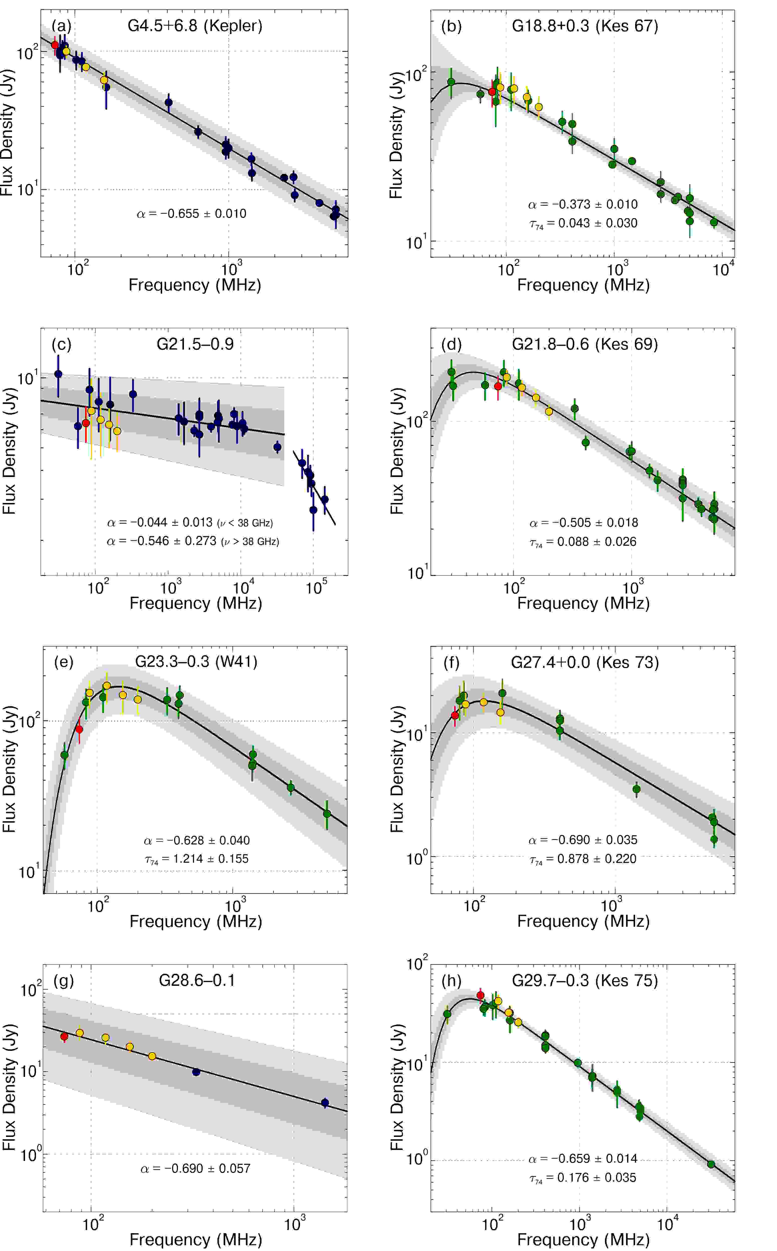
Figure 3: Revised integrated radio continuum spectra for the 14 SNRs in the VLSSr sample. In each spectrum the red filled circle indicates the new 74 MHz VLSSr flux density measurements, and the yellow ones the new GLEAM measurements. The remaining values are taken from the literature and plotted in blue or green depending on whether a single power law or a power law with a low-frequency turnover model was used to fit the data (see text for details). The solid line represents the best-fitting curve to the weighted data. Measurements were adjusted to the absolute flux density scale of Perley & Butler (2017). Gray-shaded bands represent the 1- and 2-$\sigma$ statistical uncertainty in the best-fit values of the spectral index $\alpha$ and the free-free optical depth $\tau_{74}$ (indicated in the lower portion of each panel, see also Table 3).

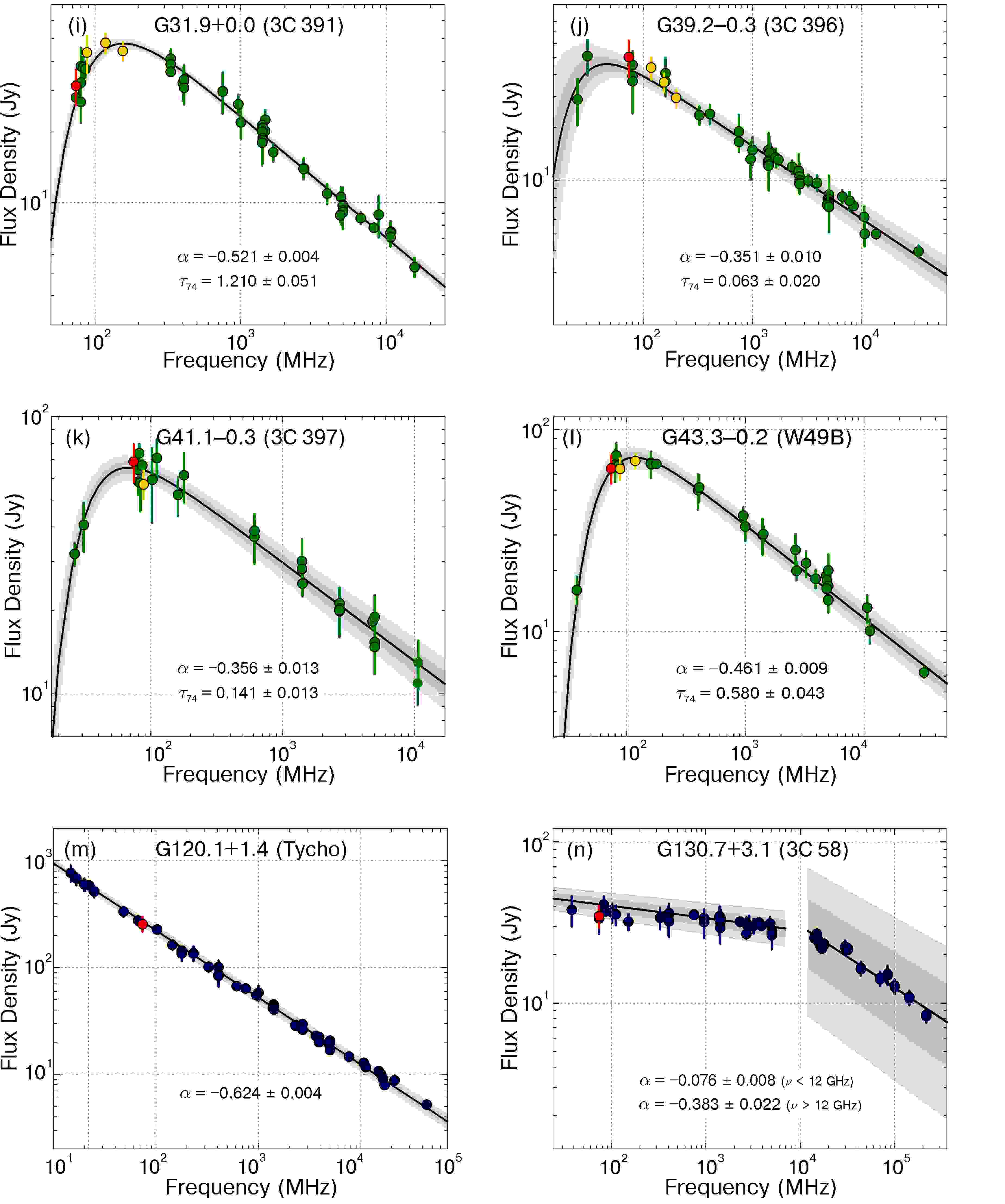
Figure 3: Continued.

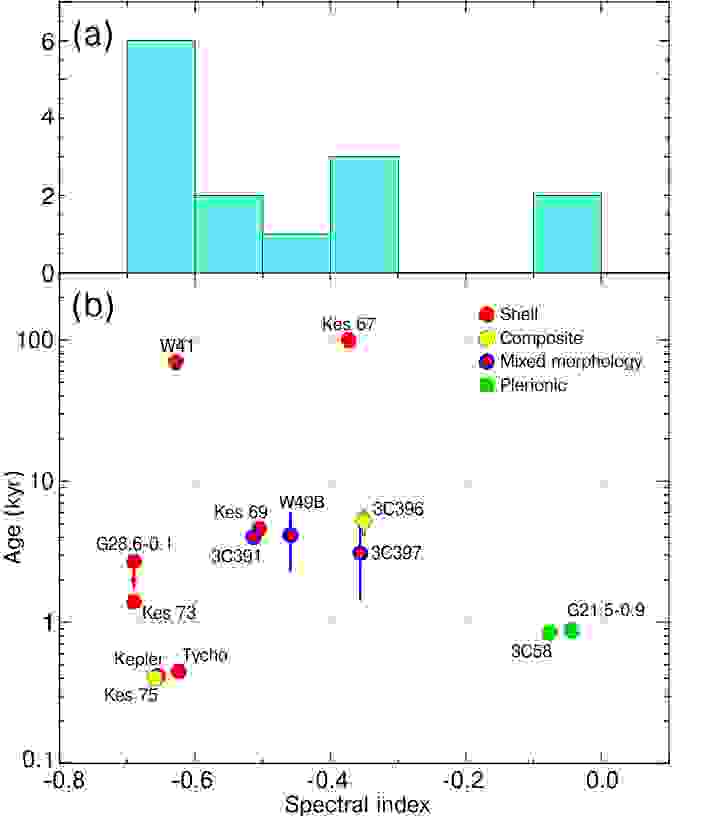
Figure 4: Panel a: Distribution of the radio continuum spectral indices as inferred from the weighted fitting to the entire spectrum of each SNR in our study (Fig. 3). Panel b: Distribution of the computed spectral index values according to the age and morphology of the source. The spectral indices for the younger ($\lesssim$3000 yr) SNRs are steeper than $-$0.5, the canonical value in test-particle diffusive shock acceleration theory.

Table 3: Radio continuum spectral index, free-free optical depth at 74 MHz, and ISM properties – emission measures ($\mathrm{EM}$) and electronic densities ($n_{\mathrm{e}}$) – computed from our fit to the spectra presented in Fig. 3.

Absorption from extended envelopes of normal HII regions (EHEs)
Source (alias)	New results					Literature
	$\alpha$	$\tau_{74}$	$\mathrm{EM}$	$n_{\mathrm{e}}$		$\alpha$	$\tau_{74}$	Refs.
			[cm-6 pc]	[cm-3]
G18.8 $+$ 0.3  (Kes 67)	$-0.373\pm 0.010$	$0.043\pm 0.030$	$150\pm 130$	$1.2\pm 0.6$		$-0.46$ - $-0.42$	$0.06\pm 0.03$	1, 2; 1
G21.8 $-$ 0.6  (Kes 69)	$-0.505\pm 0.018$	$0.088\pm 0.026$	$440\pm 140$	$2.1\pm 0.3$		$-0.56$ - $-0.50$	$0.11\pm 0.04$	1, 2; 1
G29.7 $-$ 0.3  (Kes 75)	$-0.659\pm 0.014$	$0.176\pm 0.035$	$870\pm 190$	$2.9\pm 0.3$		$-0.73$ - $-0.59$	$0.11\pm 0.04$	1, 3; 1
G41.1 $-$ 0.3  (3C 397)	$-0.356\pm 0.013$	$0.141\pm 0.013$	$720\pm 70$	$2.7\pm 0.2$		$-0.59$ - $-0.46$	$0.13\pm 0.01$	1, 2, 4; 1
Absorption: Special cases
Source (alias)	New results					Literature
	$\alpha$	$\tau_{74}$	$\mathrm{EM}$	$n_{\mathrm{e}}$		$\alpha$	$\tau_{74}$	Refs.
			[cm-6 pc]	[cm-3]
G23.3 $-$ 0.3  (W41)	$-0.628\pm 0.040$	$1.214\pm 0.155$	10 $\times$ 103	60		$-0.63$ - $-0.48$	$1.04\pm 0.11$	1, 5; 1
G27.4 $+$ 0.0  (Kes 73)	$-0.690\pm 0.035$	$0.878\pm 0.220$	8 - 15 $\times$ 103	70 - 100		$-0.71\pm 0.11$	$0.72\pm 0.32$	1; 1
G31.9 $+$ 0.0  (3C 391)	$-0.521\pm 0.004$	$1.210\pm 0.051$	600 - 2500	10 - 40		$-0.54$ - $-0.49$	$1.1$	1, 2, 6; 6
G39.2 $-$ 0.3  (3C 396)	$-0.351\pm 0.010$	$0.063\pm 0.020$	—	—		$-0.53$ - $-0.34$	$0.12\pm 0.04$	1, 2, 4, 7; 1
G43.3 $-$ 0.2  (W49B)	$-0.461\pm 0.009$	$0.580\pm 0.043$	6 - 19 $\times$ 103	$500$		$\simeq$$-0.47$	$0.14\pm 0.05$	1, 2; 8

No absorption
Source (alias)	New results		Literature
	$\alpha$		$\alpha$	Refs.
G4.5 $+$ 6.8   (Kepler)	$-0.655\pm 0.010$		$-0.65$ - $-0.62$	1, 9
G21.5 $-$ 0.9	$\left\{\begin{array}[]{c}-0.044\pm 0.013\hskip 8.5359pt\nu\lesssim 38\leavevmode\nobreak\ \mathrm{GHz}\\ -0.546\pm 0.273\hskip 8.5359pt\nu>38\leavevmode\nobreak\ \mathrm{GHz}\end{array}\right.$		$\leavevmode\nobreak\ \leavevmode\nobreak\ \begin{array}[]{c}-0.09\leavevmode\nobreak\ \mbox{-}\leavevmode\nobreak\ {+}0.08\\ -0.57\leavevmode\nobreak\ \hbox{-}\leavevmode\nobreak\ {-}0.37\end{array}$	$\leavevmode\nobreak\ \leavevmode\nobreak\ \begin{array}[]{c}1,2,10,11,12\\ 4,12\end{array}$
G28.6 $-$ 0.1	$-0.690\pm 0.057$		$-0.6$ - $-0.5$	13
G120.1 $+$ 1.4  (Tycho)	$-0.624\pm 0.004$		$-0.65$ - $-0.58$	1, 2, 9, 14, 15
G130.7 $+$ 3.1  (3C 58)	$\left\{\begin{array}[]{c}-0.076\pm 0.008\hskip 8.5359pt\nu\lesssim 12\leavevmode\nobreak\ \mathrm{GHz}\\ -0.383\pm 0.022\hskip 8.5359pt\nu>12\leavevmode\nobreak\ \mathrm{GHz}\end{array}\right.$		$\leavevmode\nobreak\ \leavevmode\nobreak\ \begin{array}[]{c}-0.10\leavevmode\nobreak\ \hbox{-}\leavevmode\nobreak\ {-}0.04\\ -0.58\leavevmode\nobreak\ \hbox{-}\leavevmode\nobreak\ {-}0.45\end{array}$	$\leavevmode\nobreak\ \leavevmode\nobreak\ \begin{array}[]{c}1,2,11,14,16,17\\ 17,18\end{array}$

4.2 Comparison to the literature

Two large samples of integrated spectra for Galactic SNRs may be found in the literature, both with flux density measurements on the absolute scale of Baars et al. (1977). Kovalenko et al. (1994b) (hereinafter referred to as K94) compiled spectra for 102 SNRs and Sun et al. (2011) (S11) compiled spectra for 50 sources. Before presenting the individual analysis for the sources in our list, we first examine general differences and agreements between the spectral properties reported in these two works and ours. The K94 sample includes spectra for 13 of the 14 SNRs in our sample, and the S11 sample includes 10 SNRs from our list. Although both works include the two PWNe from our VLSSr sample, K94 did not consider any spectral breaks in the spectrum, and S11 placed the break points for fitting the high and low frequency spectral components at different frequencies than our analysis. This makes comparisons to either work difficult, and we exclude them in the subsequent discussion. Among the remaining 11 sources which appear in both the K94 and VLSSr samples, we have found a significant discrepancy in the spectral indices for 3C 396 and 3C 397. Our analysis yields flatter values for both by $\sim 0.1$, which is 10 times larger than the uncertainty in our spectral fits for these sources. Spectral indices for the rest of the sources agree within the errors of the two measurements. This is partly due to the relatively large errors (typically 7-25%) reported on the spectral indices estimated by K94.

Among the eight sources (excluding the PWNe G21.5$-$0.9 and 3C 58) which appear in both the S11 and VLSSr samples, three of the S11 spectral indices match our new values within the reported errors (SNRs Kes 75, 3C 396, and W49B), while the rest of their determinations (SNRs Kes 67, Kes 69, 3C 391, 3C 397, and Tycho) show differences with ours. We notice that for 3C 391 the disagreement between our result and that of these authors arises from the fact that they modelled the spectrum of the source with a break at $\nu\sim 1$ GHz. We also highlight that the spectra in S11 are limited to measurements at frequencies $\nu>180$ MHz. This avoids the identification of low frequency turnovers, which can be used to probe the properties of the ionised gas. Concerning the errors in S11 spectral indices, they are comparable to those we have found in this work and range from $\sim$2 to 5%.

Details of the literature values for specific sources are included in the individual source discussions in the next section.

5 Image and spectral analysis of individual objects

In this section, we focus on the surface brightness distribution revealed in the spatially resolved VLSSr images of our sample, interpreted in the context of their integrated and local continuum spectra.

Kepler’s SNR (G4.5+6.8): Even though numerous multi-wavelength studies from the optical to the X-ray bands have been published on this remnant, its properties at low radio frequencies remain poorly explored to date (Sankrit et al., 2016, and references therein). In the VLSSr image (Fig. 1a) Kepler’s SNR consists of a roughly spherical shell structure of about 5^′ in size. The highest emissivity comes from the northwest and accounts for about 40% of the total flux density at 74 MHz ($S_{74}=111\pm 17$ Jy, Table1). In contrast to higher frequency observations, a ridge of emission connecting the southeast region with the central part of the SNR is not evident at 74 MHz (Matsui et al., 1984; DeLaney et al., 2002). Although the eastern and western ‘ears” observed at $\sim$1.4 and $\sim$4.8 GHz (DeLaney et al., 2002) appear to be missing, this is due to the lower resolution of the 74 MHz image, which is not sufficient to distinguish them. Emission in these regions is detected at 4 $\sigma$ ($\sim$ 0.9 Jy beam^-1) significance.

Fig. 2a shows the spectral index map for SNR Kepler that we have created by combining the 74 MHz-VLSSr and the 1.4 GHz NVSS images. The spectral index values range from $\sim-0.53$ to $\sim-0.75$, which is consistent with what was reported by DeLaney et al. (2002) between 1.5 and 5 GHz. In our low-frequency spectral map the flattest indices are measured in the western side of Kepler SNR.

A single power law slope $\alpha=-0.655\pm 0.010$ adequately fits the compiled flux densities measured between 74 MHz and 5 GHz (Fig. 3a). This result, consistent within uncertainties with that from Reynolds & Ellison (1992) and with what DeLaney et al. (2002) found above 1 GHz, contradicts the natural expectation from test particle calculations for flat-spectrum emission produced by fast shocks in a young object where either non-linear effects (e.g. Reynolds & Ellison 1992, Ferrand et al. 2014b) or quasi-perpendicular magnetic field configurations become important (e.g., Ferrand et al. 2014a).

Reynolds & Ellison (1992) fit the integrated radio spectrum of Kepler SNR using a non-linear shock model with a small positive curvature that gradually flattens from $\sim$30 MHz to 10 GHz ($\alpha_{<1\mathrm{GHz}}=-0.684\pm 0.024$ and $\alpha_{>1\mathrm{GHz}}=-0.586\pm 0.063$). The data used in the Reynolds & Ellison (1992) spectrum include a point at 30 MHz for which a substantially large flux excess is observed, when compared with the value obtained by extrapolating the higher radio frequency estimates. This measurement, originally reported by Jones & Finlay (1974), is the continuum peak flux density per synthesised beam for Kepler taken from an aperture synthesis survey of the Galactic plane carried out with the Fleurs observatory. The data have relatively low sensitivity, and an angular resolution ($\sim$ $0.^{\circ}8$), which is much larger than the $5^{\prime}$ source diameter. We thus feel that the measurement has a high probability of being overestimated, and have chosen to exclude it from the literature data used to construct our new spectrum, shown in Fig. 3a. We find $\alpha_{<1\mathrm{GHz}}=-0.627\pm 0.018$ and $\alpha_{>1\mathrm{GHz}}=-0.753\pm 0.046$ from the fits to our new spectrum for frequencies below and above 1 GHz, respectively. Although the higher frequency spectral index is slightly steeper, we do not feel there is convincing evidence for a spectral curvature based on the available data. More high quality data at the lowest frequencies are needed to better define any potential curvature.

SNR Kes 67 (G18.8+0.3): At 74 MHz this source has an elongated shape with a major axis length of $\sim$17^′ and a mean width of 14^′ (see Fig. 1b). The brightest emission at 74 MHz occurs on its eastern periphery. Overall the low-frequency surface brightness distribution resembles that observed at 1.4 GHz using multiple configurations of the VLA (Dubner et al., 1996). We note a plume of faint non-thermal emission extends beyond the northeast part of the shell, and is observed at a 4-$\sigma$ noise level in the VLSSr map only. The reality of this feature is questionable without further observations, and we did not include it when estimating the integrated flux density at 74 MHz listed in Table 1.

We have analysed variations in the local spectral index of the radio continuum emission from Kes 67 using the 74-MHz VLSSr and the 1.4 GHz MAGPIS images (see Fig. 2b). The measured values range from $\sim-0.15$ to $\sim-0.4$. The flattening dominating the northeastern border is consistent with a blast wave running into molecular material (Dubner et al., 2004), while the values towards the southeastern portion seem to align with HII regions (Paron et al., 2012).

We fitted the integrated flux density values between 30.9 MHz and 8.4 GHz using a power law with an exponential turnover, shown in Fig. 3b, obtaining a spectral index $\alpha=-0.373\pm 0.010$. This value is consistent, within errors, with that measured between the same range of frequencies by K94 ($\alpha=-0.42\pm 0.11$), but has a significantly lower error. On the other hand, S11 used a pure power law with a slope of $\alpha=-0.46\pm 0.02$ to fit the spectrum of this source from 330 MHz to 8.4 GHz, which is steeper than both our fit and that of K94. The discrepancy points to the importance of low frequency measurements in accurate spectral fits.

SNR G21.5$-$0.9: Emission from this well-known Crab-like SNR has been detected in radio, infrared, and X-ray bands (see, for instance Bietenholz et al., 2011; Zajczyk et al., 2012; Nynka et al., 2014; Hitomi Collaboration et al., 2018). First discovered in the 1970’s (Wilson & Weiler, 1976), the VLSSr and the GLEAM images are the highest quality that have been published for this source at frequencies below 330 MHz. As revealed in Fig. 1c, at low-radio frequencies the source has an elliptical structure with the axis of symmetry running approximately 30^∘ clockwise from the north-south direction, while radio imaging at 5 GHz (Bietenholz et al., 2011) and in X-rays (Matheson & Safi-Harb, 2010) show that this elongation runs the same amount in the opposite direction. At higher radio frequencies and X rays, G21.5$-$0.9 has an irregular structure with granular and patchy features. These fine spatial structures are not resolved at the VLSSr angular resolution.

The spectral index image in Fig. 2c was constructed from maps of the radio emission at 74 MHz and 1.4 GHz from VLSSr and NVAS, respectively. It shows a relatively uniform distribution over G21.5$-$0.9. The spectral inversion in the southwest region could represent a signature of thermal absorption from [FeII] 1.64 $\mu$m line-emitting material detected behind the shock (Zajczyk et al., 2012).

Figure 3c shows the most complete version of the G21.5$-$0.9 integrated synchrotron radio spectrum presented to date, along with a broken power-law fit. A power law with slope $\alpha=-0.044\pm 0.013$ matches the flat spectrum of the photons radiating from $\sim$57 MHz to 32 GHz. The spectrum becomes considerably steeper $\alpha=-0.546\pm 0.273$ at higher frequencies. Our analysis indicates that the break occurs at a frequency near 38 GHz, though the spectrum is poorly sampled between $\sim$11 and 70 GHz. The only detection reported in this range is at 32 GHz. The gap between the lower and higher portion in the radio continuum spectrum of G21.5$-$0.9 complicates a precise determination of the spectral break. Previously, using only a data point at 1 GHz together with microwave measurements, Planck Collaboration et al. (2016) reported a break frequency at 40 GHz, which they associated with synchrotron cooling in a source with continuous energy injection. More recently Xu et al. (2019), using a limited number of radio fluxes together with X-ray estimates, claimed evidence for spectral steepening at 50 GHz. They attributed this spectral shape to two competing mechanisms, adiabatic stochastic acceleration (ASA) and synchrotron cooling, at low (in the radio band) and high (X-ray band) energies, respectively. New radio continuum observations filling the gap at intermediate radio frequencies are required to properly determine the spectral form. A precise determination of the spectral break in conjunction with an age estimate could constrain the magnetic field strength, independent of equipartition assumptions.

SNR Kes 69 (G21.8$-$0.6): This remnant is an incomplete shell at 74 MHz with the surface brightness fading from the eastern to the western side of the remnant (see Fig. 1d). The HII region G021.884$-$00.318 towards the northwest of the SNR shell (Anderson et al., 2014) appears in absorption in the VLSSr map, which is expected for this kind of object as they become optically thick at low radio frequencies against the Galactic non-thermal background (Nord et al., 2006). To our knowledge, no electron temperatures have been reported for the thermal source. Working constraints can be obtained through the relation presented in Quireza et al. (2006), derived from an electron temperature gradient in the Galactic disk, $T_{\mathrm{e}}=(5780\pm 350)+(287\pm 46)\,R_{\mathrm{Gal}}$, where $R_{\mathrm{Gal}}$ is the Galactocentric distance to the HII region. For G021.884$-$00.318 placed at $\sim$10.7 kpc (Anderson et al., 2014), we have $R_{\mathrm{Gal}}\simeq 4.2$ kpc, and thus this implies a characteristic $T_{\mathrm{e}}\simeq 7000$ K. For an optically thick HII region, the cosmic ray emissivity of the column behind the thermal gas can be measured from the excess of the observed brightness temperature of the HII region over its electron temperature (see Polderman et al. 2019 and references therein for a thorough treatment of this topic). Assuming the HII region G021.884$-$00.318 is resolved at our spatial resolution, the maximum depth of the absorption at 74 MHz, in brightness temperature, is $-$6500 K. This measurement is important for Galactic cosmic ray physics and can add to the growing catalogue of HII absorption regions (Polderman et al., 2020).

Figure 2d displays the spectral index distribution over Kes 69 obtained between the 74 MHz and 1.4 GHz maps from VLSSr and MAGPIS surveys respectively. There seems to be a general trend of flattening from northwest to southeast ($\alpha\sim-0.4$ to $-0.2$). This is compatible with the molecular shell in the vicinity of the remnant detected by Zhou et al. (2009).

The integrated spectral slope for Kes 69 indicates a low-frequency turnover (Fig. 3d) suggestive of foreground thermal absorption, an issue we revisit in Sect. 6. The weighted fit to our compiled flux densities results in a radio spectral index $\alpha=-0.505\pm 0.018$, in good agreement with the value $-0.5\pm 0.11$ from K94, but somewhat discrepant with the S11 value of $\alpha=-0.56\pm 0.03$ derived from a power-law fit to measurements at $\nu>$ 330 MHz. We note that part of the thermal emission from the HII region G021.884$-$00.318 could have been included in earlier, low-resolution flux density measurements of Kes 69 at frequencies higher than 74 MHz. However, since this HII region contributes only $\sim 1$ Jy at GHz frequencies, its impact on the accuracy of the integrated SNR spectra is minimal.

SNR W41 (G23.3$-$0.3): The VLSSr image shown in Fig. 1e clearly reveals the elongated $\sim$18^′ western part of the SNR shell, with a highly irregular boundary and enhanced knots of emission at several locations. Radio continuum imaging at 1.4 GHz shows a weak arm emerging from the northern part of the western edge, extended about 20^′ to the east, which has been interpreted as a non-thermal component of the radio emission that originates from W41 (Leahy & Tian, 2008). Traces of this northern W41 arm also appear in the GLEAM Survey, with a synthesised beam of 5${}^{\prime}.6\times 5^{\prime}.3$ at 88 MHz (Wayth et al., 2015; Hurley-Walker et al., 2019). However we do not see any corresponding weak emission in the VLSSr map above 4 $\sigma$ significance. Using this non-detection to set a limit on the spectral index for this emission, we estimate that this feature would contribute $\lesssim$10 % to the integrated flux density of W41 at 74 MHz, which is well within the reported measurement errors.

Figure 2e displays the spatial variations in the 74 MHz-1.4 GHz spectral index of the radio continuum emission created from VLSSr and MAGPIS images. The picture showing, on average, $\alpha\sim-0.35$ flat spectrum is consistent with the thermal gas in the region of the remnant. In Sect. 6.3, we further discuss the relative geometry of W41 and the ISM constituents near and towards it as discerned from its radio continuum spectrum.

The integrated spectral index from our spectrum in Fig. 3e is $\alpha=-0.628\pm 0.040$. Although our value is steeper than $\alpha=-0.48\pm 0.14$ reported in K94, there is no significant differences because of the large uncertainty on their value. We are confident that our result represents a more reliable estimation, since our spectrum is better sampled, especially at frequencies lower than 200 MHz.

Thermal sources of varying sizes ($0^{\prime}.7$ - $6^{\prime}.5$) within the area of this remnant are included in the WISE Catalog of Galactic HII regions (Anderson et al., 2014). These sources have been mapped in previously published radio continuum images of W41 at frequencies higher than 74 MHz (e.g. 330 MHz, Kassim 1992; 1.4 GHz, Leahy & Tian 2008). Therefore, it is highly probable that contamination from this thermal gas has limited a precise estimate of the flux of the synchrotron emission from the remnant in that portion of the radio spectrum.

SNR Kes 73 (G27.4+0.0): Originating $\lesssim 2000$ yr ago from a core-collapse SN event, Kes 73 is one of the youngest SNRs in the Galaxy (Borkowski & Reynolds, 2017). The VLSSr image shows a slightly asymmetric shell with a bright, nearly point-like spot (Fig. 1f). The position of this feature at R.A$\simeq$$18^{\mathrm{h}}\,41^{\mathrm{\leavevmode\nobreak\ }{m}}\,15^{\mathrm{s}}.6$, Decl.$\sim$$-04^{\circ}\,56^{\prime}\,59^{\prime\prime}$ does not coincide with the magnetar 1E 1841$-$045 thought to be the compact remnant of the stellar explosion that created G27.4+0.0 (Kumar et al., 2014, and references therein). From the current image it is not possible to tell if it is part of the SNR or an unrelated background source. In the latter case, we note that it contains $\simeq$ 12% of the total flux from Kes 73, well within the errors on the measured total flux.

The local distribution of the radio spectrum over the SNR, calculated between 74 MHz and 1.4 GHz from the comparison of VLSSr and MAGPIS images, is on average flatter than the integrated spectral index value (Fig. 2f). It can be explained, however, in terms of the ionised material in the region of the remnant. A detailed consideration of the interstellar medium properties in connection with the radio emission from Kes 73 is presented in Sect. 6.3.

The inclusion of the 74 MHz flux density in the integrated continuum spectrum (Fig. 3f) supports the low-frequency turnover inferred in Kovalenko et al. (1994a) and Kassim (1989a). The fit to the flux measurements is overplotted in Fig. 3f (although the 30.9 MHz upper limit appears in the spectrum it was excluded from the fit). We find a spectral index $\alpha=-0.690\pm 0.035$, in good agreement with the result in K94.

SNR G28.6$-$0.1: This source has been poorly studied in the radio band since its identification as a Galactic SNR with a broken morphology (Helfand et al., 1989). The VLSSr map of G28.6$-$0.1 shows three bright connected structures (see Fig. 1g). The absence of 74-MHz emission from nearby sources located at the northwest of the SNR is consistent with their thermal nature as first proposed by Helfand et al. (1989) and confirmed later by Anderson et al. (2011). The spectral index image in Fig. 2g constructed using 74-MHz VLSSr and 1.4 GHz MAGPIS data, reveals a striking flattening to the southeast. The near-IR image of G28.6$-$0.1 presented by Lee et al. (2019) shows some [FeII] thin filaments in this portion of the remnant, thought to be created by a radiative shock front moving through the ambient medium.

Despite the paucity of literature flux density measurements, VLSSr, GLEAM, 330 MHz and 1.4 GHz measurements are adequate to constrain a fit to the continuum spectrum with a single power-law with index $\alpha=-0.690\pm 0.057$ (see Fig. 3g). To measure the impact of the ionised material on the integrated continuum spectrum of the source, more sensitive observations below 100 MHz are needed.

SNR Kes 75 (G29.7$-$0.3): Kes 75 is one of the strongest radio sources in our sample. The 74-MHz map shown in Fig. 1h reveals an elliptically-shaped SNR with the brightest radio emission found on the southwestern part of the shell. There is no evidence for the PWN powered by the PSR J1846$-$0258 (Gotthelf et al., 2000) in the VLSSr image. In contrast to most higher-frequency total-intensity radio images (e.g. at 1.4 and 89 GHz in Bock & Gaensler, 2005), the full northern extent of the shell is visible in the VLSSr image.

The spectral index map of Kes 75 between the VLSSr at 74 MHz and MAGPIS at 1.4 GHz is displayed in Fig. 2h. The southwest region of the remnant has an $\alpha\leavevmode\nobreak\ \sim\leavevmode\nobreak\ -0.4$, flatter than that of its surroundings by $\sim$+0.2. This spectral component corresponds to a location where the SN shock is running into a molecular shell and the brightness in radio continuum, X rays and mid-IR is strongest.

From the spectrum of Kes 75 plotted in Fig. 3h, the 30.9 MHz flux density lies below the general trend of the data, suggesting a low frequency turnover (see also Sect. 6). Excluding a turnover, the spectral index $\alpha=-0.659\pm 0.014$ from our integrated spectrum is consistent with values found in both K94 and S11.

SNR 3C 391 (G31.9+0.0): The VLSSr 74-MHz continuum image of 3C 391 presented in Fig. 1i clearly shows a bright rim on the western side of the remnant, while towards the eastern half of the source the emission is dimmer. This picture is consistent with VLA imaging by Brogan et al. (2005) at both 330 MHz and 74 MHz, in which they attribute localised absorption in this SNR to the interaction zone between the SNR and its immediate environment. They conclude that the thermal absorbing gas was created by the impact of a dissociative shock from the SNR with the molecular cloud with which it is interacting.

The spectral index map for 3C 391 between the emission at 74 MHz from VLSSr and at 1.4 GHz from MAGPIS is displayed in Fig. 2i. The trend of spectral flattening is consistent with Brogan et al. (2005)’s interpretation of a SNR interacting with a molecular cloud.

The integrated spectrum of 3C 391 shows a robust low-frequency turnover (Fig. 3i), which is seen in multiple low-frequency measurements. Our spectral index $\alpha=-0.521\pm 0.004$ after combining the new VLSSr flux density measurements with previous published values (excluding the 30.9 MHz upper limit) is completely consistent with earlier results derived by Brogan et al. (2005) and K94. We do not find evidence for two straight power laws with a frequency break at 1 GHz, which was presented in S11. We notice that the data points below 1 GHz in their spectrum are notoriously more scattered than ours. We favour the low frequency turnover over the broken power law fit, since the plotted measurements that meet our selection criteria show a clear smooth curve at low frequencies.

SNR 3C 396 (G39.2$-$0.3): The radio emission from this remnant has been almost exclusively mapped above 1 GHz (Cruciani et al., 2016, and references therein). To the best of our knowledge, the 74-VLSSr image (see Fig. 1j) is the highest resolution sub-GHz view of this source presented to date. The source was imaged at 330 MHz by Kassim (1992) using the VLA, but was only marginally resolved. Lower angular resolution images of 3C 396 from GLEAM at 88, 118, 155, and 188 MHz are available as well. In the VLSSr map the SNR appears considerably distorted from circular symmetry.

A bright ridge of emission extends from south to north, with a knot $\sim$1.4 times brighter than its surroundings. Between this position and a second radio enhancement further north, lies the non-thermal X-ray emission attributed to a central pulsar wind nebula powered by a putative pulsar (Olbert et al., 2003). As is also observed at higher frequencies, the radio emission of 3C 396 gradually fades from west to east. A blowout tail towards the northeastern portion of the SNR shell and curving around to the west was visible in the radio domain using 1.4 GHz data (Patnaik et al., 1990). It is also observed as an extended bright structure in the Spitzer MIPSGAL image at 24 $\mu$m (Reach et al., 2006). It is not visible in the 74 MHz VLSSr image, which supports the thermal emission mechanisms proposed to explain its origin, and is unlikely to be part of the SNR (Anderson & Rudnick, 1993). Furthermore, there is no structure in the VLSSr 74-MHz map which corresponds to the southwest extension noticeable in the earlier 330 MHz study of Kassim (1992). We have the sensitivity to see this feature, but owing to its non-detection in the VLSSr image we conclude it is either thermal or due to confusion.

The spectral index map of 3C 396 between 74 MHz and 1.4 GHz using VLSSr and VGPS data is presented in Fig. 2j. Variations in the spectrum are recorded from about $\alpha\sim-0.3$ up to $\sim\leavevmode\nobreak\ -0.6$. The flattest spectral feature occurs towards the southwestern corner of the remnant, a region where both [FeII] and H₂ near-IR line emission have been detected, indicating a SNR shock interacting with a dense medium (Lee et al., 2019). Additional details of the thermal gas responsible for the spectral characteristics of 3C 396 are presented in Sect. 6.3.

The integrated radio spectrum of 3C 396 is shown in Fig. 3j. The fit to the set of data with a power law and an exponential turnover model yields a spectral index $\alpha=-0.351\pm 0.010$. Our determination agrees well with the global spectral index reported in S11 ($\sim-0.34$) and Cruciani et al. (2016) ($\sim-0.364$). In these three cases the spectra include high frequency fluxes up to $\sim$33 GHz. We also notice that our result (and hence those from S11 and Cruciani et al. 2016) differs from the global spectral index derived by K94 ($\sim-0.48$). We believe the spectrum presented in K94 is less reliable because the lack of measurements at frequencies higher than 10.6 GHz.

SNR 3C 397 (G41.1$-$0.3): As seen in Fig. 1k, the morphology of this SNR at 74 MHz follows the box-like shape observed at higher radio frequencies (e.g. Dyer & Reynolds, 1999). The brightest region is on the west side of the source and contains $\sim 30$% of the total flux density measured at 74 MHz (see Table 1). Publicly available images for this source at 1.4GHz do not include the full flux density reported in the literature, so we have not constructed a spectral index map for it.

As noticed by Dyer & Reynolds (1999), confusion with thermal emission from an HII region just west of the SNR (since catalogued as G041.126$-$00.232, Anderson et al. 2014) likely prevented accurate non-thermal measurements of the SNR by many lower resolution instruments which are reported in the literature. The spectral index $\alpha=-0.356\pm 0.013$ that we have fit (Fig. 3k) is hardly compatible with the $-0.46\pm 0.10$ value reported in K94, but it is considerably flatter than the spectrum $\alpha=-0.50\pm 0.01$ measured by S11 using a pure power-law fit to a much less complete set of flux density measurements.

SNR W49B (G43.3$-$0.2): The VLSSr 74-MHz image in Fig. 1l shows a roughly circular source, approximately $5^{\prime}$.5 in diameter, with considerably brightened emission on the eastern part of the shell. The spectral map created from the 74 MHz VLSSr and 1.4 GHz MAGPIS images is shown in Fig. 2k. There is a dramatic flattening from the northeast ($\alpha\sim\leavevmode\nobreak\ -0.8$) to the southwest portions of W49B ($\alpha\sim\leavevmode\nobreak\ -0.15$). Overall the distribution of spectral index shows the same trends as in Lacey et al. (2001).

A spectral turnover for $\nu\lesssim 100$ MHz in the integrated spectrum is well known and has been linked by Lacey et al. (2001) to foreground thermal gas superimposed over the western half of the remnant. The low-frequency thermal absorption is very distinctive in the new spectrum shown in Fig. 3l, and the derived value of the global spectral index $\alpha=-0.461\pm 0.009$ is consistent with the spectral fit by Lacey et al. (2001). In Sect. 6.3 we readdress the analysis of the thermal gas responsible for the absorption implied by the radio spectrum of W49B.

Tycho’s SNR (G120.1+1.4): The VLSSr low-frequency image of this rim-brightened shell-type SNR agrees with previously published images at higher radio frequencies (e.g. Katz-Stone et al., 2000). Figure 1m displays a roughly circular shell of $\sim$9^′ in diameter with a highly non-uniform emission. There is some departure from circular symmetry in the southeast. A brightening is especially prominent in the northeastern portion of the SNR where the peak surface brightness is $\sim$14 Jy beam^-1. This enhancement could be produced by the northeast front of the shell impinging the inner boundary of the wind-blown molecular bubble, the latter revealed in ¹²CO $J=2-1$ line observations (Zhou et al., 2016). As with all classic rim-brightened shell-type SNRs, the interior emission is much more diffuse. Overall, the surface brightness distribution in the VLSSr image of Tycho is also in reasonably good agreement with that observed with LOFAR in the 58-143 MHz range (Arias et al., 2019b). Fig. 2l displays the spatial spectral variations across Tycho SNR, obtained from VLSSr and NVAS data at 74 MHz and 1.4 GHz, respectively. Our spectral index map nicely picks out and confirms the internal absorption observed by Arias et al. (2019b) with the LOw Frequency ARray (LOFAR).

The integrated radio spectrum is shown in Fig. 3m, based on data collected over more than three decades from $\sim$15 MHz to 70 GHz. It yields a relatively steep integrated spectrum $\alpha=-0.624\pm 0.004$, largely consistent with the previous determination reported by K94 but incompatible with that of S11 ($-0.58\pm 0.02$). Alternatively, Reynolds & Ellison (1992) modelled the emission from Tycho at frequencies up to $\sim$10 GHz with a modest spectral break in the power law of $\Delta\alpha\simeq 0.04$ at 1 GHz, inferring an underlying curved spectrum. Power-law fits to our data below and above the inferred break yield slopes of $\alpha_{<1\leavevmode\nobreak\ \mathrm{GHz}}=-0.607\pm 0.012$ and $\alpha_{>1\leavevmode\nobreak\ \mathrm{GHz}}=-0.581\pm 0.010$, respectively. This is weakly consistent with an intrinsically curved, underlying concave-up spectrum.

The steep radio spectral index and suggested curvature in this remnant have been attributed by several authors to non-linear effects in the acceleration process of the radio-emitting electrons (e.g. Reynolds & Ellison 1992, Völk et al. 2008). Wilhelm et al. (2020) recently presented an alternative explanation, suggesting the entire spectrum, from radio to $\gamma$-rays, can be reproduced in terms of stochastic re-acceleration in the immediate downstream region of the SNR forward shock, without invoking the consequences of non-linear particle acceleration kinetic theory.

SNR 3C 58 (G130.7+3.1): 3C 58 represents the archetypal example of a pulsar-powered plerion.

In the 74 MHz image (Fig. 1n), it appears elongated in the east-west direction, with a size of approximately $8^{\prime}.5\times 4^{\prime}.5$, similar to that observed at higher radio frequencies and even in X rays (Slane et al., 2004; Bietenholz, 2006).

Due to the limited spatial resolution, the VLSSr image does not resolve the complex of loop-like features seen throughout the nebula at higher radio frequencies, but shows a bright component at the location of the pulsar PSR J0205+6449, and a brightness distribution that gradually fades with radial distance from the centre. The morphology of the spectral index between 74 MHz and 1.4 GHz from the VLSSr and NVAS images, respectively, is shown in Fig. 2m. It matches the flat and uniform 74/327 MHz and 327 MHz/4.9 GHz spectral index distributions presented by Bietenholz et al. (2001b).

The integrated spectrum is presented in Fig. 3n and includes measurements at frequencies from 38 MHz to 217 GHz, with a notable gap between $\sim 5$ and $\sim$14 GHz. The best-fit to the data points from 38 MHz to 5 GHz results in a synchrotron spectral index $\alpha=-0.076\pm 0.008$, in agreement with previous studies (see, for instance, Green & Scheuer 1992, Kovalenko et al. 1994a or Sun et al. 2011), while measurements above 14 GHz are better fit by a considerably steeper power-law index $\alpha=-0.383\pm 0.022$. From our analysis, a spectral break occurs at $\sim$12 GHz, somewhat lower than the break reported by Planck Collaboration et al. (2016). However, within the uncertainties, our result is compatible with the value $\sim$18 GHz provided by Xu et al. (2019), which results from the fit to a broadband (from radio to X rays) spectrum of 3C 58. As in the case of G21.5$-$0.9, an interplay of synchrotron cooling and re-acceleration of electrons in the pulsar wind nebula through the ASA process was used by Xu et al. (2019) to explain the observed spectral shape. Adding new radio measurements in the 5-14 GHz gap is critical to refining the spectral break in 3C 58.

6 Analysis of the Low Frequency Spectral Turnovers

6.1 General Considerations

Turnovers in the low frequency ($\nu\lesssim 100$ MHz) continuum spectra of SNRs were first identified in the 1970’s and attributed to external thermal absorption by an ionised component of the ISM along the line of sight (see e.g. Dulk & Slee, 1975a). With a larger sample, Kassim (1989a) attributed the observed patchiness of the absorption to low-density, intervening extended HII region envelopes (EHEs), the existence of which had been inferred earlier from stimulated, meter-wavelength radio recombination lines (Anantharamaiah, 1986). In the 1990’s intrinsic SNR thermal absorption was first detected in Cas A due to unshocked ejecta (Kassim et al., 1995), from thermal filaments in the Crab Nebula (Bietenholz et al., 1997), and much more recently in Tycho with LOFAR (Arias et al., 2019b). A third possible source of thermal absorption is ionised gas resulting from physical processes in the immediate surroundings of SNRs. All three cases are important because they provide critical distance constraints for disentangling the relative superposition of ionised gas and SNRs.

One of the earliest detections of resolved thermal absorption towards a Galactic SNR was made at the relatively high frequency of 330 MHz in the special case of the Galactic centre, through the detection of Sgr A West against the Sgr A East SNR (Anantharamaiah et al., 1991). Thereafter followed W49B, the earliest typical case of resolved foreground absorption, attributed to an EHE enveloping a complex of HII regions along the line of sight (Lacey et al., 2001). By contrast and also within the VLSSr sample, 3C 391 represents the first detection of resolved thermal absorption at the interface of a SNR blast wave interacting with a molecular cloud (Brogan et al., 2005).

In this section we use our spectral fits of the eight SNRs in our sample exhibiting turnovers to constrain the properties of the absorbing thermal gas.

6.2 Absorption by Intervening Ionised Gas

In four cases (Kes 67, Kes 69, Kes 75, and 3C 397, see Table 3), we can easily attribute the moderately low optical depths and higher levels of absorption at lower frequencies to the generic case of foreground ionised gas which is not associated with the SNRs. For simplicity we assume that EHEs are the most likely source of this gas, but we note that other manifestations of intervening ionised gas could also cause the absorption.

To estimate the physical properties of the intervening ionised gas we can make use of the relation between the optical depth at a reference frequency, $\tau_{\nu_{0}}$, the electron temperature of the thermal gas $T_{\mathrm{{e}}}$, and the emission measure $\mathrm{EM}=\displaystyle{\int_{L}}n_{\mathrm{e}}^{2}\,dx$, which depends in turn on the electron density, $n_{\mathrm{e}}$, and the linear extent $L$ along the line of sight. Setting the singly-ionised species, $Z_{\mathrm{i}}=n_{\mathrm{e}}/n_{\mathrm{i}}=1$, we have the expression (Wilson et al., 2009)

$$\tau_{\nu_{0}}=3.014\times 10^{-2}\left(\frac{T_{\mathrm{e}}}{\mathrm{K}}\right)^{-3/2}\left(\frac{\nu_{0}}{\mathrm{GHz}}\right)^{-2}\,g_{\mathrm{ff}}\,\left(\frac{\mathrm{EM}}{\mathrm{pc\leavevmode\nobreak\ cm^{-6}}}\right),$$ (2)

where $g_{\mathrm{ff}}$ is the Gaunt factor:

$$g_{\mathrm{ff}}=\mathrm{ln}\left[4.955\times 10^{-2}\left(\frac{\nu_{0}}{\mathrm{GHz}}\right)^{-1}\right]+1.5\,\mathrm{ln}\left(\frac{T_{\mathrm{e}}}{\mathrm{K}}\right).$$ (3)

For the four spectral turnover cases we attribute to line of sight absorption, we adopt generic EHE electron temperatures and path lengths of 5000 K and 100 pc, respectively (Kassim, 1989a), inferring the EM and electron densities reported in Table 3. These are consistent with properties inferred independently from RRLs free of discrete continuum sources (Anantharamaiah, 1985), as expected given that the generic EHE properties from Kassim (1989a) were also consistent with the RRL results.

6.3 Absorption by associated ionised gas

Interpretation of the remaining SNRs with low-frequency spectral turnovers is less clear. EHE absorption seems questionable to account for the relatively high optical estimate for W41, while infrared (IR) and molecular line emission from Kes 73, 3C 396 and W49B show intriguing correspondence with their non-thermal radio emission. The SNR 3C 391 also shows evidence of correlation between IR and non-thermal radio emission. Because it has been studied in depth by Brogan et al. (2005), and our new spectra are consistent with their results, we do not discuss it further here.

For SNRs Kes 73 and W49B, we construct free-free optical depth maps using the relation $\tau_{\mathrm{74}}=\ln\left(S_{\mathrm{exp}}/S_{\mathrm{obs}}\right)$, where $S_{\mathrm{obs}}$ is the observed 74 MHz emission, while $S_{\mathrm{exp}}$ is the emission expected if no absorption is present. To create the $S_{\mathrm{exp}}$ maps we scale the 1.4 GHz images from the literature to the expected 74 MHz fluxes using the integrated radio spectral indices of each source (Kes 73, $\alpha\simeq-0.69$ and W49B, $\alpha\simeq-0.46$, see Table 3). The extrapolated images are convolved to match the 75^′′ resolution of the VLSSr images, and masked at the 4-$\sigma$ level based on their respective noise. Based on reasonable assumptions for the electron temperatures, we convert the $\tau_{\mathrm{74}}$ distributions into local EM measurements based on Eq. 2. An important assumption in the extrapolation from 1.4 GHz to 74 MHz is that measured spectral deviations are dominated by foreground thermal absorption and not by intrinsic variations in the spectrum of the synchrotron emitting electrons, which are typically much more subtle.

6.3.1 SNR W41

Figure 5 shows the mid-IR emission from GLIMPSE and the MIPS Galactic Plane Survey (Carey et al., 2009) in color with superimposed radio emission contours for SNR W41. There are numerous HII regions with line-of-sight coincidence with the W41 SNR, many of which overlap the 1.4 GHz emission (green contours). The remnant and probably the majority of these HII regions are part of the giant molecular cloud G23.0$-$0.4 (Hogge et al. 2019, and references therein). For HII regions A-H (see Fig. 5) the association with the SNR is readily accepted because their previously established distances (e.g. from radio recombination lines, Chen et al. 2020) are consistent with that of the remnant ($4.8\pm 0.2$ kpc, Ranasinghe & Leahy 2018). No distance measurements have been reported for the remaining HII regions I-Z.

Compared to the emission at 1.4 GHz, the 74 MHz VLSSr emission is significantly attenuated on the eastern side of the remnant (white contours in Fig. 5) and bears striking testimony to thermal absorption. This is consistent with the prevalence of HII regions on the eastern side of the complex. While this indicates that many of these HII regions (and any associated EHEs) must be in the foreground relative to the SNR, this need not be the case for all of them. For example HII regions E and M could be background to the SNR, since they appear almost coincident with regions where the 74 MHz emission is not attenuated. Nevertheless, on the basis of the VLSSr image we are able to place an independent upper limit $\sim$5 kpc to a significant subset of these HII regions, based on the SNR distance. Future observations are required to precisely place all the HII regions relative to the SNR, but it would not be surprising if they are all roughly at the same distance and associated with the G23.0$-$0.4 giant molecular cloud complex.

To estimate the physical characteristics of the ionised gas responsible for absorbing the 74 MHz SNR emission, we first derive the electron temperature by using the relation between magnitude and the Galactocentric distance to the source (Quireza et al. 2006, more detail given in the analysis of G21.8$-$0.6 SNR in Sect. 5). For the complex of HII regions in which W41 is embedded at an assumed $\sim$5 kpc heliocentric distance, we find a characteristic $T_{\mathrm{e}}\simeq 7100$ K. Under the high-opacity approximation, valid for low-frequency radio measurements, we calculate the average brightness temperature of the synchrotron emission behind the thermal gas of $T_{\mathrm{B}}\sim 6000$ K. Future RRL observations are required to better constrain the electron temperatures, but we note that our rough estimate is consistent with those measured in typical HII regions (Luisi et al., 2019).

Assuming that the ionised gas can be characterised by a single electron temperature, we can derive the average EM corresponding to the absorbing gas from Eq. 2, using the measured optical depth from our best-fit model to the SNR spectrum ($\tau_{\mathrm{74}}\sim 1.2$). We derived a mean $\mathrm{EM}\simeq 10\times 10^{3}$ pc cm^-6, comparable to the values typically measured in other known HII regions (Luisi et al., 2019). This result can be used to estimate the electron density of the absorbing gas using the observed geometry. If we consider a path-length $L\sim 4$ pc through the ionised gas, equivalent to the mean linear size of the overlapping HII regions (angular diameters ranges from $\sim$$1^{\prime}.5$ to $\sim$$7^{\prime}.5$), then the resulting average electron density is $n_{\mathrm{e}}\simeq 60$ cm^-3 (Table 3). This density likely represents a blend of absorption from denser HII region cores and their associated lower density EHEs.

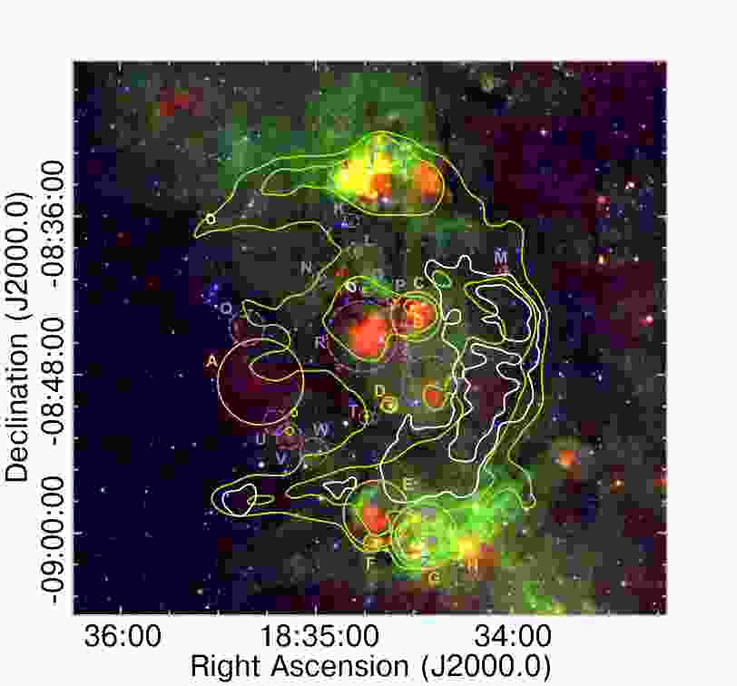
Figure 5: Spitzer 3-colour image (RGB: 24, 8.0, and 3.6 $\mu$m) towards the SNR W41’s complex with contours of radio continuum emission overlaid. Green contours (at 0.25 and 0.42 Jy beam^-1 levels) correspond to the 1.4 GHz image from MAGPIS, convolved to match the VLSSr resolution of $75^{\prime\prime}$. VLSSr 74 MHz continuum contours are superimposed in white (levels: 0.56 and 1.30 Jy beam^-1). Multiple HII regions, A-H, in the field with known distances near W41 ($\sim$5 kpc) are marked by orange circles, while thermal sources (I-Z) with unknown distance are indicated by dashed violet circles (Anderson et al., 2014).

6.3.2 SNR Kes 73

Kes 73 is very bright at 24 $\mu$m, and this emission is completely coincident with the SNR radio shell as shown in Fig. 6a. Taking the properties of the observed mid-IR features into consideration, Carey et al. (2009) argued it could predominantly arise from [OIV] and [FeII] line emission. Later, Pinheiro Gonçalves et al. (2011) attributed the IR radiation in Kes 73 to dust grains heated by collisions in the hot plasma behind the SNR shock front. The emission is analogous to other known SNR molecular cloud interactions in which ionised atomic species created after the passage of a dissociating SNR shock produce abundant line emission in the mid-IR (e.g. RCW 103, W44, W28, 3C 391, Oliva et al. 1999; Reach & Rho 2000).

The striking coincidence of the mid-IR emission with the 1.4 GHz radio emission is consistent with the low frequency spectral turnover depicted in Fig. 3f. We hypothesise that the turnover can be plausibly attributed to absorption by ionised gas in a molecular cloud that is either in the process of being enveloped by the SNR shock wave or has already been impacted by it. This interpretation is supported by near-IR [FeII]-emitting ($\sim$1.6 $\mu$m) clumps detected in the southern part of Kes 73; these were interpreted to be shocked circumstellar gas rather than high-speed metal-enriched SN ejecta (Lee et al., 2019).

The scenario of a SNR-molecular cloud interaction is supported by Fig. 6b, which depicts the integrated intensity map from the Boston University-FCRAO Galactic Ring Survey (GRS, Jackson et al. 2006) in the velocity range $v_{\mathrm{LSR}}$= 95-105 km s^-1 overlaid with the mid-IR (cyan contours) and 74 MHz radio continuum (yellow contours) emission. The plotted molecular emission includes the velocity corresponding to the $\sim$5.8 kpc kinematic distance to Kes 73 recently revised by Ranasinghe & Leahy (2018) and Lee et al. (2020). A bright portion of the CO cloud is spatially coincident with the SNR, with molecular emission also extending to the northwest of Kes 73. Around the peak of the cloud we find features with a velocity width of $\sim$8-10 km s^-1. Most of the mid-IR gas shows good spatial correlation with the molecular gas, especially towards the west. It is noteworthy that the molecular structure mapped here is not consistent with the previous study by Liu et al. (2017), who considered molecular gas at a distance of 9 kpc associated with the western ($\sim$90 km s^-1) and northwestern ($\sim$85-88 km s^-1) boundaries of the remnant.

To test the reliability of our idea that the observed absorption is tracing ionised gas in the cloud interacting with the SNR, we examined the characteristics of the absorption by locally mapping the free-free continuum optical depth at 74 MHz across Kes 73. To do this, we used the 74-MHz VLSSr and the 1.4 GHz-MAGPIS image of the remnant.

As shown in Fig. 6c the optical depth varies by a factor of $\sim 3$ across the source, with average errors in $\mathrm{\tau_{74}}$ of   25%. Mid-IR emission contours from Spitzer at 24 $\mu$m are superposed on the $\tau_{74}$ optical depth map, generally indicating IR emission widely distributed across the high optical depth features. The mid-IR displays a saddle shape, with peaks to the east and west, and a minimum near the centre. The optical depth map mimics this morphology, exactly as expected if the region of highest mid-IR emission corresponds to the region of strongest low frequency absorption (a similar effect was seen in 3C 391 by Brogan et al. 2005). Note that the IR contours lying outside of the eastern boundary of the optical map correspond to a very low surface brightness region at 74 MHz, which was clipped for the construction of the optical depth map.

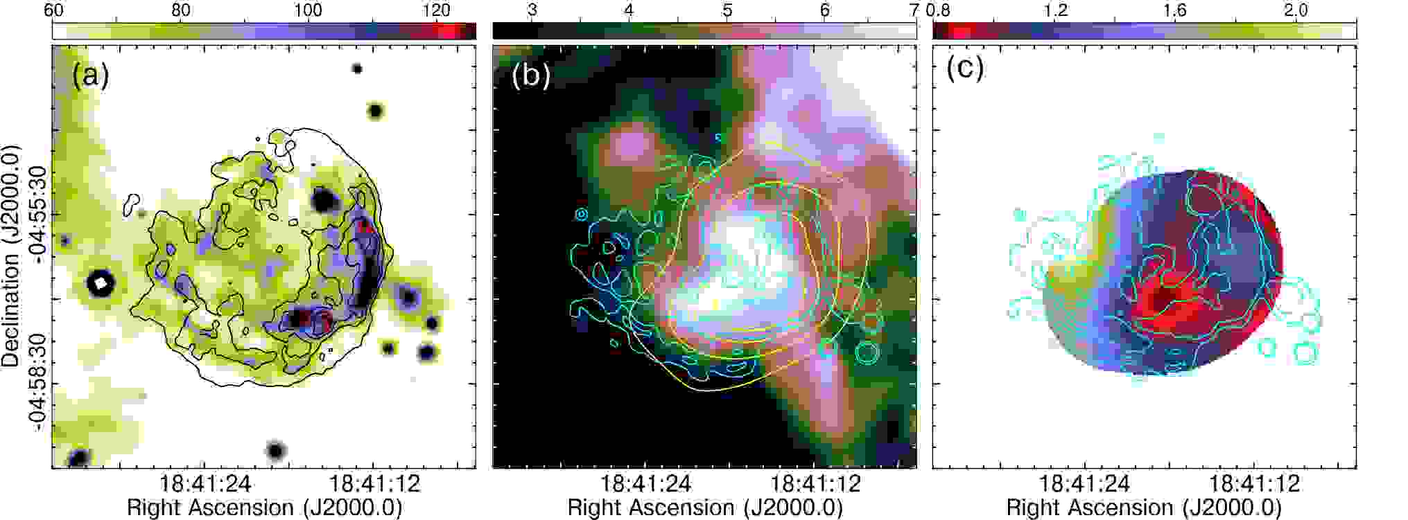
Figure 6: Panel a: Spitzer MIPSGAL 24 $\mu$m image for SNR Kes 73 (shown with a linear colour scale in MJy sr^-1) overlaid with black contours tracing 1.4 GHz radio continuum emission at levels 2.5, 4.8, 7.6, and 11 mJy beam^-1 from the MAGPIS survey. The morphology of the IR emission strongly mimics the radio emission. Panel b: ¹³CO (1-0) data from GRS integrated in the $v_{\mathrm{LSR}}$=95-105 km s^-1 range. The linear colour scale is in K km s^-1. Cyan and yellow contours represent the mid-IR (levels: 70 and 84 MJy sr^-1) and 74 MHz low-radio frequency intensities (levels: 0.8, 1.3, 1.8, and 2.2 Jy beam^-1), respectively. The newly-identified CO cloud is detected within the boundaries of the Kes 73 shell. Panel c: Optical depth towards Kes 73 at 74 MHz as a function of position. Cyan contours superimposed delineate the mid-IR emission as in panel b.

Typical electron density can be derived from the distribution of $\mathrm{EM}$ (not shown here) assuming, as is usual in the literature, that absorption occurs over a characteristic mean path length equivalent to the mean transverse extent of the region where the optical depth changes. We use this assumption to characterise the approximate range of electron densities in the ionised gas corresponding to the non-uniform absorption inferred in Fig. 6c. We measure absorption levels corresponding to characteristically high and low optical depths of 1.8 and 0.95, respectively. Furthermore we adopt $T_{\mathrm{e}}\sim 7000$ K from the mid-IR ionic line observations of interstellar shocks (Hewitt et al., 2009). Following Eq. 2 and Eq. 3 we derive local variations in $\mathrm{EM}\simeq$ 8-15 $\times 10^{3}$ pc cm^-6. Considering mean size scales ranging between $L\simeq$ 0.^′7 and 1^′ (or $\sim$1.2-1.7 pc at a distance of $\sim$5.8 kpc to Kes 73) for the optical depth variations, we obtain thermal absorbing electron densities $n_{\mathrm{e}}$=$\sqrt{\mathrm{EM}/L}\sim$ 70-110 cm^-3 for the ionised gas causing the absorption towards Kes 73. While these values are much larger than that estimated in the extended envelopes of HII regions (0.5-10 cm^-3, Kassim 1989a), they are consistent with electron densities derived from low-radio frequency data in the ionised shocked gas linked to 3C 391, an established SNR molecular cloud interaction (Brogan et al., 2005). Our estimate is similarly consistent with the electron density reported in Koo et al. (2016) ($\sim$600 cm^-3) from the analysis of mid-IR [FeII] line ratios in the shocked gas of a sample of SNRs. A partial explanation for the difference between the electron density computed here and that by Koo et al. (2016) might be that their value corresponds to a model with a shock speed 150 km s^-1, which is slower than expected for a young SNR with a relatively fast shock speed such as Kes 73 (age $\sim$1400 yr, blast wave velocity $\sim 1400\,d_{8.5}$ km s^-1 $\simeq$ 950 km s^-1, after correction by the revised 5.8 kpc SNR’s distance, Borkowski & Reynolds 2017). We note that significant variations in electron densities $\sim$100-1000 cm^-3 can be inferred from combinations of different shock models or mid-IR ionic lines ratios with modest temperature variations typically centred at $\sim$7000 K (Oliva et al., 1999; Reach & Rho, 2000; Hewitt et al., 2009; Koo et al., 2016).

We conclude that the ionised gas associated with the interaction of Kes 73 and a molecular cloud are likely to be responsible for the observed low frequency radio absorption. The absorbing gas may be ionised directly by the interaction of the shock front with the cloud, or from the SNR’s X-ray radiation (Kumar et al., 2014). Since Kes 73 is a relatively young SNR, ionization by its stellar progenitor cannot be discounted either. Finally, it is not unreasonable to consider absorption by unshocked ejecta such as is found in Cas A or Tycho SNRs (Arias et al., 2018, 2019b). However based on a spatially resolved spectroscopic X-ray study (Kumar et al., 2014) and the non-centrally condensed, widespread distribution of high optical depth across the remnant, we find this latter scenario unlikely.

6.3.3 W49B

One of the earliest examples of spatially resolved thermal absorption against a Galactic SNR was made at 74 MHz by Lacey et al. (2001). They attributed the significant attenuation towards the southwest region of the remnant to foreground absorption by intervening HII regions and their associated EHEs. The resolved absorption was consistent with the low frequency turnover in the integrated SNR spectrum (for example see Fig.  3l). The inference of intervening HII regions seemed consistent with much earlier detection of radio recombination lines by Pankonin & Downes (1976) towards W49B’s non-thermal radio shell. However much higher resolution, modern observations (c.f. Anderson et al. 2014) reveal no classic HII regions towards the western part of W49B, where Lacey et al. (2001) measured the strongest absorption. The only catalogued source is the foreground HII region WISE G043.305$-$00.211 (2^′ in size) located at 4.3 kpc (Anderson et al., 2014) towards the northeastern edge of W49B. Furthermore, Kalcheva et al. (2018) identified the thermal WISE source as an ultracompact HII region (named G043.3064$-$00.2114) with a size of 2^′′ at a distance of 4.4 kpc. Given the poor angular resolution ($\sim$8${}^{\prime}.5$, two times the SNRs’ size) of Pankonin & Downes (1976)’s observations it is probable their RRL detection emanated from the thermal source G043.305$-$00.211.

Infrared observations, presented by Keohane et al. (2007) and more recently by Lee et al. (2019), have shown that W49B is very bright in both [FeII] (1.644 $\mu$m) and $\mathrm{H_{2}}$ (2.122 $\mu$m) line emission. There is good spatial agreement between filaments emitting in ionic iron lines and the synchrotron radio shell of the SNR (see Fig. 7a), while the $\mathrm{H_{2}}$ near-IR emitting gas encloses the eastern, southern, and western SNR boundaries. There are several scenarios to explain the apparent association of [FeII] emission with W49B. They include shock interaction with material swept up by the stellar winds of the progenitor, radiative atomic shocks propagating into a dense ambient medium, photoionisation by the adjacent X-ray emission from the shock-heated ejecta, and SN ejecta with high Fe abundance (Lee et al. 2019, and references therein). While the current evidence is not sufficient to exclude X-ray heating, the $\mathrm{H_{2}}$ (2.122 $\mu$m) emission favors a shock interaction with dense material. In addition, previous studies of the large-scale ambient medium of W49B have shown molecular clouds close to the remnant (Simon et al., 2001; Zhu et al., 2014).

The considerably improved observations towards W49B since Lacey et al. (2001) suggest a significantly revised and more exciting interpretation of the low frequency observations than the chance superposition of HII regions along the line of sight. Figure 7b shows the distribution of the free-free optical depth in W49B constructed from the radio continuum emission towards the source at 74 MHz and 1.4 GHz from the VLSSr and NVSS surveys, respectively. Superposed contours trace the [FeII] near-IR line emission. The absorption levels across the SNR are high, ranging from 0.2 to 1.6. The highest absorption features are localised in the eastern and western portions of W49B (mean $\tau_{74}\sim$ 0.45 and 1.4, respectively) and show excellent correspondence with the brightest [FeII] filaments despite the limited angular resolution of the $\tau_{74}$ map. This correspondence provides strong evidence that the thermal absorption in W49B derives from a direct interaction with its environment.

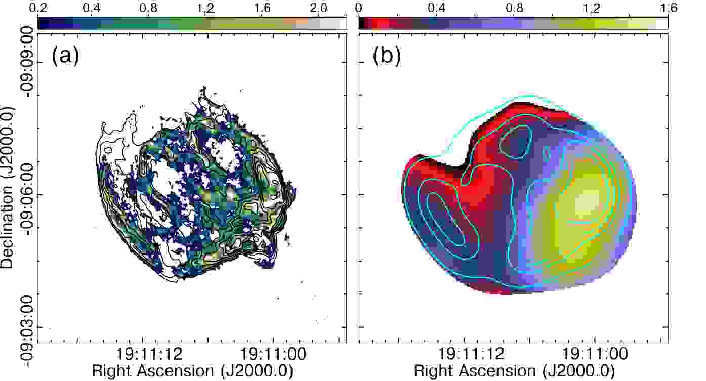
Figure 7: Panel a: [FeII] line emission at 1.644 $\mu$m towards SNR W49B (image kindly provided by Dr. Lee, Y.-H.) overlaid with contours (levels: 3, 10, 20, 30, 40, 50, and 60 mJy beam^-1) of the 1.4 GHz continuum radiation detected in the MAGPIS survey. The colour representation is linear in units of MJy sr^-1. Panel b: Local distribution of the optical depth computed towards W49B at 74 MHz. Cyan contours of the near-IR [FeII] line emission matched at the 45^′′ resolution are superimposed for comparison, with levels at 12, 47, 70, and 105 MJy sr^-1.

In order to estimate the thickness of the ionised gas layer, we analyse variations in the $\mathrm{EM}$ with position over W49B from the local values of the optical depth at 74 MHz. We adopt an electron temperature of 10⁴ K, with an electron density of $\sim$500 cm^-3 (estimated from the ionic gas in W49B by Zhu et al. 2014). Using Eq. 2 and Eq. 3, the average free-free optical depth towards the eastern and western portion of the SNR shell translate into $\mathrm{EM}$ values between 6 $\times$ 10³ and 19 $\times$ 10³ pc cm^-6, respectively. From this we conclude that the observed absorption is taking place in a thin layer with typical thickness of $L=\mathrm{EM}/n_{\mathrm{e}}^{2}$=(2.5-7.6)$\times$10^-2 pc ($\sim$0.8-2.3 $\times$10¹⁷ cm). These values, markedly narrower than the typical thickness of $\sim$5 pc measured in ISM cavities surrounding SNRs (Fukui et al., 2012), are consistent with the hypothesis that absorption of the low frequency radio emission is due to ionised material generated by the impact of the SN shock front on the wall of the bubble shaped by the winds of W49B’s progenitor star (Keohane et al., 2007).

6.3.4 3C 396

Spectroscopic observations made with Spitzer reveal multiple ionic (e.g., [FeII], [NeII], [SiII], etc.) and molecular (e.g. $\mathrm{H_{2}S(0)}$, $\mathrm{H_{2}S(1)}$, etc.) transitions across SNR 3C 396 (Hewitt et al., 2009). A very bright [FeII] ($\sim$1.6 $\mu$m) filament is observed near the southwestern boundary of the remnant along with $\mathrm{H_{2}}$ ($\sim$2.1 $\mu$m) emission extending outside of the radio and the [FeII]-line boundaries (Lee et al. 2019, and references therein). The ionic lines are indicative of a post-shock colliding region. The shocked ambient medium could be either dense clumps previously formed by the wind material of the SN progenitor (Lee et al., 2009) or a dense molecular cloud interacting with the 3C 396 blast wave (Lee et al., 2019). Su et al. (2011) claim that ¹²CO (1-0 and 2-1) molecular material at the distance of 6.2 kpc is colliding with the SNR shock front. Subsequently, Ranasinghe & Leahy (2018) revised the distance to the source to $8.5\pm 0.5$ kpc, based on HI 21 cm and ¹³CO line observations. This is roughly consistent with the $9.5\pm 0.1$ kpc estimate derived by Lee et al. (2020) from the velocities of the near-IR H₂ emission lines. Thus the interaction of 3C 396 with the ionic line emission and CO at 6.2 kpc is uncertain.

The spectral index map for this source (Fig. 2j) reveals variations on the order of $\pm$ 0.35 across 3C 396, from $-$0.26 in the south west, gradually steepening to $\alpha\sim$ $-$0.6 towards the interior of the western shell. The spectral flattening is discernible in an extension of $\sim$0.8^′ $\times$ 2^′.5 along the southwestern limb, with spectral index $-$0.26 to $-$0.35. A striking result enabled by our spatially resolved spectral index map is the correspondence between this flattest region and the bright [FeII] filament noted above, as seen in Figure  8. This immediately implies thermal absorption in the post-shock interaction region traced by the ionic line emission, reminiscent of 3C 391. It is not surprising that the integrated spectrum for this source eventually turns over at lower frequencies as the effects of the absorption grow stronger (Fig.  3i). These results show that this bright SNR, along with 3C 391, would be an excellent target for higher resolution, lower frequency observations to perform a comprehensive analysis of the correlation between the ionised IR gas and thermal absorption discerned from the radio optical depth.

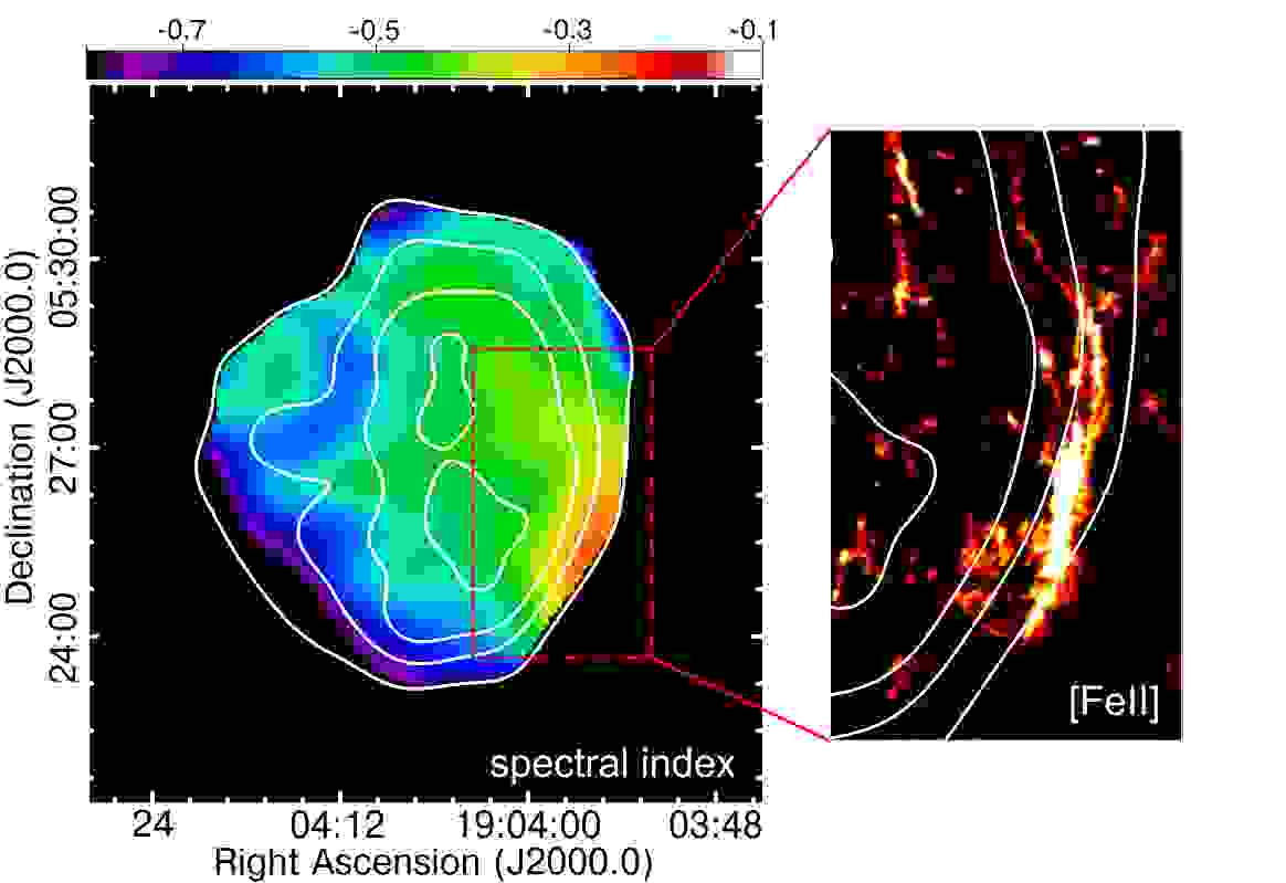
Figure 8: Comparison between the 74 MHz/1.4 GHz radio spectral index distribution over the remnant 3C 396 (the same displayed in Fig. 2) and the filaments emitting in ionic iron line emission. The flattest spectral index feature is located where the bright [FeII] near-IR filaments are observed. Contours from the 74-MHz VLSSr image at levels 0.64, 1.7, 2.5, and 3.6 Jy beam^-1 are included for reference.

7 Summary and Conclusions

We have updated the radio continuum spectra of 14 Galactic SNRs using new flux density measurements from the VLSSr and GLEAM in combination with carefully selected measurements from the literature. Where possible, measurements over the range of frequencies from 50 MHz to 50 GHz were placed on the absolute flux density scale developed by Perley & Butler (2017). The spectra were fit by power-laws, broken power-laws, and power laws with low frequency turnovers as appropriate for each source. We have measured steep spectral index values ($|\alpha|>0.5$) for the younger non-PWNe sources in our sample.

The VLSSr data independently confirm the area of absorption in the centre of the Tycho SNR seen by LOFAR LBA (Arias et al., 2019b), although the integrated spectrum is well-fit by a simple power-law without a turnover. The integrated spectra for SNR G4.5+6.8 (Kepler) and G28.6$-$0.1 are also well fit by simple power-laws, and no evidence for thermal absorption is seen. The integrated spectra for the two pulsar wind nebulae, G21.5$-$0.9 and 3C 58 (G130.7+3.1), are well fit by power-laws with spectral breaks at 38 and 12 GHz, respectively. The new integrated spectrum for SNR 3C 391 confirms the low-frequency turnover previously seen by Brogan et al. (2005).

We analyse potential free-free thermal absorption processes that cause the turnovers at frequencies below 100 MHz observed in the spectra of eight additional SNRs. We explain the curved spectra of Kes 67, Kes 69, Kes 75, and 3C 397 as thermal absorption occurring when their lines of sight intersect thermal gas, which may be diffuse ionised envelopes associated with normal HII regions.

For SNR W41, we explain the thermal absorption as arising in a number of HII regions either in close proximity to, or coincident with, the SNR. The average extension of the non-thermal radio emission in this remnant at 74 MHz is $20\%$ smaller than the combined thermal and non-thermal emission measured at 1.4 GHz. This indicates that the size of the SNR had been previously overestimated due to contamination by thermal sources.

For the three SNRs Kes 73, 3C 396, and W49B, we have found a strong spatial correspondence between the IR ionic line emission and the highest level of absorption that we measure in these sources. On the basis of this correlation and previously reported evidence for the interaction of these sources with their surroundings, we explain the free-free absorption towards these sources in terms of ionised gas created after the impact of the SN shock with the interstellar material. For Kes 73 and W49B we are able to derive electron temperatures and densities. This is similar to the interpretation of 3C 391 previously published by Brogan et al. (2005). Our study adds to a growing body of work demonstrating that physical questions about SNRs and their surroundings can be tackled by incorporating low-radio frequency observations in the analysis, since these data are a potent tool for separating thermal and non-thermal emission in complex regions.

8 Future Work

The improved accuracy of the integrated continuum spectra achieved by adding reliable measurements below 100 MHz is important to better understand the physical processes within SNRs. For example, the improved integrated spectra can help constrain theories that explain high-energy particle production in a sample of SNRs which are also bright in $\gamma$ rays (G21.5$-$0.9, W41, Kes 73, Kes 75, 3C 391, W49B, Tycho, and 3C 58). A future work, analysing the broad-band spectral distribution of these sources is in preparation and it will be presented elsewhere for publication.

Despite the progress represented in this paper, the paucity of good measurements below 100 MHz, where thermal absorption is much easier to detect, remains prevalent. There are many SNRs, e.g. Kes 75, where the inference of a low-frequency turnover relies on a single low frequency measurement. Emerging data from the LOFAR LBA Sky Survey (LoLSS: de Gasperin et al. 2021) survey, with unprecedented resolution and sensitivity below 100 MHz, should have a major impact on this field. Despite LOFAR’s limited access to the inner Galaxy and the majority of known SNRs, it should significantly increase the known population of interacting SNRs detectable through thermal absorption.

Appendix A List of integrated flux densities

Tables in this section contain the flux density measurements used in this work to model the radio continuum spectra of 14 Galactic SNRs. As indicated in their third columns, the listed values include new low frequency fluxes that we calculated from the VLSSr and GLEAM projects, along with measurements from previous publications. We applied correction factors to adjust the fluxes between 50 MHz and 50 GHz to the absolute flux density scale of Perley & Butler (2017), the frequency range over which the scale is valid with an accuracy of 3%-5%. We notice that, out of the 454 flux densities listed in our work, only about 6% have not been placed in the Perley & Butler (2017) scale because they correspond to either frequencies lower than 50 MHz or higher than 50 GHz. Additionally, for a small fraction (14%) of the fluxes a determination of the correction factor was not possible because information on the primary flux calibrators was not recorded in the original reference.

Table 4: Integrated flux densities compiled for the SNR G4.5+6.8, used to trace the spectrum presented in Fig. 3a.

G4.5+6.8 (Kepler)
Frequency	Scaled flux	Reference
$[$MHz$]$	density [Jy]
74	111 $\pm$ 17	This work (from VLSSr)
80	98.4 $\pm$ 9.6	Dulk & Slee (1972)
80	100.9 $\pm$ 30.3	Slee (1977)
80	93.6 $\pm$ 7.6	Dulk & Slee (1975b)
83	104.4 $\pm$ 14.9	Kovalenko et al. (1994a)
86	110.0 $\pm$ 22.0	Mills et al. (1960)
88	100.0 $\pm$ 9.0	This work (from GLEAM)
102	86.8 $\pm$ 12.8	Kovalenko et al. (1994a)
111	84.7 $\pm$ 12.8	Kovalenko et al. (1994a)
118	77.0 $\pm$ 7.0	This work (from GLEAM)
155	62.0 $\pm$ 9.0	This work (from GLEAM)
160	55.0 $\pm$ 16.5	Slee (1977)
408	42.6 $\pm$ 6.4	Dulk & Slee (1972)
635	26.2 $\pm$ 2.6	Milne & Hill (1969)
960	21.2 $\pm$ 2.9	Harris (1962)
960	18.8 $\pm$ 2.0	Harris & Roberts (1960)
960	21.2 $\pm$ 0.5	Trushkin (1998)
1000	20.0 $\pm$ 3.0	Milne (1970)
1410	16.7 $\pm$ 1.7	Milne & Hill (1969)
1420	13.2 $\pm$ 1.6	Lequeux (1962)
2300	12.2 $\pm$ 0.3	Trushkin (1998)
2650	12.3 $\pm$ 1.2	Milne & Hill (1969)
2700	9.1 $\pm$ 0.9	Milne & Dickel (1974)
3900	8.0 $\pm$ 0.2	Trushkin (1998)
4850	6.4 $\pm$ 0.3	Griffith et al. (1994)
5000	6.6 $\pm$ 1.3	Milne & Dickel (1975)
5000	7.2 $\pm$ 1.1	Dulk & Slee (1972)

Table 5: Integrated flux densities compiled for the SNR G18.8+0.3, used to trace the spectrum presented in Fig. 3b.

G18.8+0.3 (Kes 67)
Frequency	Scaled flux	Reference
$[$MHz$]$	density [Jy]
30.9	87.4 $\pm$ 17.5	Kassim (1988)
57.5	73.9 $\pm$ 8.2	Odegard (1986)
74	76.2 $\pm$ 13.8	This work (from VLSSr)
80	84.1 $\pm$ 11.8	Slee & Higgins (1973)
80	66.9 $\pm$ 19.1	Dulk & Slee (1972)
83	86.5 $\pm$ 19.9	Kovalenko et al. (1994a)
88	81 $\pm$ 17	This work (from GLEAM)
111	78.8 $\pm$ 19.7	Kovalenko et al. (1994a)
118	80 $\pm$ 14	This work (from GLEAM)
155	71 $\pm$ 11	This work (from GLEAM)
160	67.7 $\pm$ 10.1	Dulk & Slee (1975b)
200	62 $\pm$ 9	This work (from GLEAM)
330	50.8 $\pm$ 7.6	Kassim (1992)
408	38.9 $\pm$ 5.8	Kesteven (1968)
408	49.2 $\pm$ 7.4	Kassim (1989b)
960	28.3 $\pm$ 0.3	Trushkin (1998)
1000	35.0 $\pm$ 5.3	Milne (1970)
1465	29.7 $\pm$ 0.3	Dubner et al. (1996)
2695	18.9 $\pm$ 1.9	Altenhoff et al. (1970)
2700	22.3 $\pm$ 3.3	Milne & Dickel (1974)
3650	17.4 $\pm$ 0.3	Trushkin (1998)
3900	18.3 $\pm$ 0.3	Trushkin (1998)
4800	15.1 $\pm$ 0.9	Sun et al. (2011)
5000	17.9 $\pm$ 3.6	Milne & Dickel (1975)
5000	14.6 $\pm$ 2.2	Milne (1969)
5000	13.1 $\pm$ 2.6	Reifenstein et al. (1970)
8400	12.9 $\pm$ 1.0	Milne et al. (1989)

Table 6: Integrated flux densities compiled for the SNR G21.5$-$0.9, used to trace the spectrum presented in Fig. 3c.

G21.5$-$0.9
Frequency	Scaled flux	Reference
$[$MHz$]$	density [Jy]
30.9	10.4 $\pm$ 2.1	Kassim (1988)
57.5	6.2 $\pm$ 1.2	Kassim (1989b)
74	6.4 $\pm$ 1.1	This work (from VLSSr)
83	8.9 $\pm$ 2.0	Kovalenko et al. (1994a)
88	7.2 $\pm$ 2.7	This work (from GLEAM)
111	7.9 $\pm$ 2.0	Kovalenko et al. (1994a)
118	6.6 $\pm$ 2.0	This work (from GLEAM)
155	6.3 $\pm$ 1.3	This work (from GLEAM)
160	7.7 $\pm$ 2.3	Slee (1977)
200	5.9 $\pm$ 1.1	This work (GLEAM)
330	8.5 $\pm$ 1.3	Kassim (1992)
1400	6.7 $\pm$ 1.0	Frail & Moffett (1993)
1660	6.5 $\pm$ 1.3	Milne (1969)
2300	5.9 $\pm$ 0.3	Trushkin (1998)
2700	5.7 $\pm$ 1.1	Milne (1969)
2700	6.9 $\pm$ 0.7	Milne & Dickel (1974)
2700	7.0 $\pm$ 0.4	Becker & Kundu (1976)
2700	6.8 $\pm$ 1.4	Goss & Day (1970)
3900	6.2 $\pm$ 0.3	Trushkin (1998)
4800	6.4 $\pm$ 0.4	Sun et al. (2011)
4875	6.9 $\pm$ 1.0	Downes et al. (1980)
5000	6.7 $\pm$ 1.3	Reifenstein et al. (1970)
5000	6.7 $\pm$ 0.3	Bietenholz & Bartel (2008)
5000	6.1 $\pm$ 1.8	Altenhoff et al. (1970)
7700	6.3 $\pm$ 0.3	Trushkin (1998)
8100	7.0 $\pm$ 0.4	Becker & Kundu (1976)
8900	6.2 $\pm$ 0.9	Caswell & Clark (1975)
10600	6.4 $\pm$ 0.7	Becker & Kundu (1976)
11200	6.0 $\pm$ 0.3	Trushkin (1998)
32000	5.0 $\pm$ 0.3	Morsi & Reich (1987)
70000	4.3 $\pm$ 0.6	Planck Collaboration et al. (2016)
84000	3.9 $\pm$ 0.7	Salter et al. (1989b)
90700	3.8 $\pm$ 0.4	Salter et al. (1989a)
94000	3.5 $\pm$ 0.4	Bock et al. (2001)
100000	2.7 $\pm$ 0.5	Planck Collaboration et al. (2016)
143000	3.0 $\pm$ 0.4	Planck Collaboration et al. (2016)

Table 7: Integrated flux densities compiled for the SNR G21.8$-$0.6, used to trace the spectrum presented in Fig. 3d.

G21.8$-$0.6 (Kes 69)
Frequency	Scaled flux	Reference
$[$MHz$]$	density [Jy]
29.9	210 $\pm$ 40	Jones & Finlay (1974)
30.9	170.6 $\pm$ 34.1	Kassim (1988)
57.5	172.4 $\pm$ 34.5	Kassim (1989b)
74	169.0 $\pm$ 31.0	This work (from VLSSr)
83	208.8 $\pm$ 39.8	Kovalenko et al. (1994a)
88	194 $\pm$ 21	This work (from GLEAM)
111	177.2 $\pm$ 39.4	Kovalenko et al. (1994a)
118	166 $\pm$ 20	This work (from GLEAM)
155	143 $\pm$ 16	This work (from GLEAM)
200	116 $\pm$ 14	This work (from GLEAM)
330	121.4 $\pm$ 18.2	Kassim (1992)
408	73.0 $\pm$ 7.3	Shaver & Goss (1970b)
960	63.7 $\pm$ 6.1	Trushkin (1998)
1000	64.0 $\pm$ 9.6	Milne (1970)
1414	47.9 $\pm$ 4.8	Altenhoff et al. (1970)
1660	41.5 $\pm$ 6.2	Milne (1969)
2700	41.0 $\pm$ 8.2	Milne (1969)
2700	31.7 $\pm$ 9.2	Willis (1973)
2700	42.1 $\pm$ 4.6	Velusamy & Kundu (1974)
2700	39.6 $\pm$ 7.9	Milne & Dickel (1974)
2700	38.5 $\pm$ 7.7	Goss & Day (1970)
3650	29.1 $\pm$ 2.9	Trushkin (1998)
3900	27.0 $\pm$ 2.9	Trushkin (1998)
4800	23.7 $\pm$ 1.3	Sun et al. (2011)
4875	26.7 $\pm$ 4.0	Downes et al. (1980)
5000	23.1 $\pm$ 4.6	Kundu et al. (1974)
5000	29.0 $\pm$ 5.8	Milne & Dickel (1975)
5000	27.1 $\pm$ 5.4	Goss & Shaver (1970)

Table 8: Integrated flux densities compiled for the SNR G23.3$-$0.3, used to trace the spectrum presented in Fig. 3e.

G23.3$-$0.3 (W41)
Frequency	Scaled flux	Reference
$[$MHz$]$	density [Jy]
57.5	59.2 $\pm$ 11.8	Kassim (1989b)
74	88.0 $\pm$ 17.0	This work (from VLSSr)
83	133.2 $\pm$ 29.8	Kovalenko et al. (1994a)
88	154 $\pm$ 30	This work (from GLEAM)
111	143.7 $\pm$ 29.5	Kovalenko et al. (1994a)
118	172 $\pm$ 40	This work (from GLEAM)
155	149 $\pm$ 37	This work (from GLEAM)
200	139 $\pm$ 28	This work (from GLEAM)
330	138.7 $\pm$ 27.7	Kassim (1992)
400	130.0 $\pm$ 26.0	Downes (1971)
408	148.6 $\pm$ 22.3	Kesteven (1968)
1400	50.0 $\pm$ 10.0	Downes (1971)
1414	52.1 $\pm$ 5.2	Altenhoff et al. (1970)
1420	59.7 $\pm$ 8.2	Tian et al. (2007)
2695	35.9 $\pm$ 3.6	Altenhoff et al. (1970)
5000	24.6 $\pm$ 2.5	Altenhoff et al. (1970)
5000	24.0 $\pm$ 5.0	Downes (1971)

Table 9: Integrated flux densities compiled for the SNR G27.4+0.0, used to trace the spectrum presented in Fig. 3f.

G27.4+0.0 (Kes 73)
Frequency	Scaled flux	Reference
$[$MHz$]$	density [Jy]
74	13.8 $\pm$ 2.5	This work (from VLSSr)
80	18.2 $\pm$ 5.5	Slee (1977)
85.7	20.0 $\pm$ 6.0	Mills et al. (1958)
88	17.0 $\pm$ 3.5	This work (from GLEAM)
118	17.6 $\pm$ 2.9	This work (from GLEAM)
155	14.6 $\pm$ 3.0	This work (from GLEAM)
160	20.9 $\pm$ 6.3	Slee (1977)
408	10.4 $\pm$ 1.6	Caswell et al. (1982)
408	13.0 $\pm$ 2.0	Kassim (1989b)
408	12.6 $\pm$ 1.9	Kesteven (1968)
1415	3.5 $\pm$ 0.5	Caswell et al. (1982)
4850	2.1 $\pm$ 0.1	Griffith et al. (1994)
5000	1.9 $\pm$ 0.2	Haynes et al. (1978)
5000	1.9 $\pm$ 0.5	Angerhofer et al. (1977)
5000	1.4 $\pm$ 0.2	Milne (1969)

Table 10: Integrated flux densities compiled for the SNR G28.6$-$0.1, used to trace the spectrum presented in Fig. 3g.

G28.6$-$0.1
Frequency	Scaled flux	Reference
$[$MHz$]$	density [Jy]
74	26.9 $\pm$ 4.7	This work (from VLSSr)
88	29.5 $\pm$ 5.6	This work (from GLEAM)
118	25.9 $\pm$ 3.9	This work (from GLEAM)
155	20.2 $\pm$ 3.1	This work (from GLEAM)
200	15.5 $\pm$ 1.9	This work (from GLEAM)
330	9.9 $\pm$ 0.8	Supan et al. (2012)
1420	4.2 $\pm$ 0.5	Supan et al. (2012)

Table 11: Integrated flux densities compiled for the SNR G29.7$-$0.3, used to trace the spectrum presented in Fig. 3h.

G29.7$-$0.3 (Kes 75)
Frequency	Scaled flux	Reference
$[$MHz$]$	density [Jy]
30.9	31.2 $\pm$ 6.2	Kassim (1988)
74	48.5 $\pm$ 7.9	This work (from VLSSr)
80	35.3 $\pm$ 4.8	Dulk & Slee (1975c)
83	36.8 $\pm$ 7.0	Kovalenko et al. (1994a)
102	38.5 $\pm$ 10.8	Kovalenko et al. (1994a)
111	40.4 $\pm$ 11.8	Kovalenko et al. (1994a)
118	42.3 $\pm$ 6.5	This work (from GLEAM)
155	32.4 $\pm$ 3.4	This work (from GLEAM)
160	26.9 $\pm$ 6.7	Slee (1977)
160	31.9 $\pm$ 5.2	Dulk & Slee (1975c)
200	25.5 $\pm$ 2.7	This work (from GLEAM)
408	19.0 $\pm$ 1.9	Shaver & Goss (1970a)
408	14.0 $\pm$ 1.4	Shaver & Goss (1970b)
408	18.5 $\pm$ 2.8	Green (1974)
408	15.0 $\pm$ 2.2	Dulk & Slee (1972)
408	15.0 $\pm$ 2.3	Kassim (1989b)
960	9.9 $\pm$ 0.9	Trushkin (1998)
1400	7.0 $\pm$ 1.4	Downes (1971)
1414	7.3 $\pm$ 2.2	Altenhoff et al. (1970)
2695	5.0 $\pm$ 1.5	Altenhoff et al. (1970)
2700	5.3 $\pm$ 0.5	Milne & Dickel (1974)
4800	3.6 $\pm$ 0.6	Sun et al. (2011)
4875	2.8 $\pm$ 0.3	Downes et al. (1980)
5000	3.4 $\pm$ 0.3	Milne (1969)
5000	3.2 $\pm$ 0.5	Downes (1971)
5000	3.4 $\pm$ 0.5	Dulk & Slee (1972)
32000	0.9 $\pm$ 0.1	Morsi & Reich (1987)

Table 12: Integrated flux densities compiled for the SNR G31.9+0.0, used to trace the spectrum presented in Fig. 3i.

G31.9+0.0 (3C 391)
Frequency	Scaled flux	Reference
$[$MHz$]$	density [Jy]
74	31.5 $\pm$ 5.4	This work (from VLSSr)
74	28.1 $\pm$ 1.8	Brogan et al. (2005)
80	26.9 $\pm$ 5.0	Caswell et al. (1971)
80	38.2 $\pm$ 7.6	Dulk & Slee (1975c)
80	32.5 $\pm$ 4.8	Dulk & Slee (1972)
83	37.8 $\pm$ 4.0	Kovalenko et al. (1994a)
86	37.2 $\pm$ 2.8	Artyukh et al. (1969)
88	43.7 $\pm$ 8.0	This work (from GLEAM)
118	48.1 $\pm$ 4.9	This work (from GLEAM)
155	44.4 $\pm$ 4.1	This work (from GLEAM)
330	38.9 $\pm$ 0.3	Brogan et al. (2005)
330	41.1 $\pm$ 4.0	Kassim (1992)
330	36.1 $\pm$ 0.5	Moffett & Reynolds (1994)
400	32.4 $\pm$ 5.2	Kellermann (1964)
408	30.9 $\pm$ 4.6	Kesteven (1968)
408	33.5 $\pm$ 5.0	Green (1974)
408	33.5 $\pm$ 2.9	Caswell et al. (1971)
408	33.1 $\pm$ 5.0	Kassim (1989a)
750	29.9 $\pm$ 6.0	Holden & Caswell (1969)
750	29.8 $\pm$ 1.5	Pauliny-Toth et al. (1966)
750	29.8 $\pm$ 3.0	Kellermann et al. (1969)
960	26.3 $\pm$ 2.5	Trushkin (1998)
1000	22.0 $\pm$ 3.3	Milne (1970)
1400	20.1 $\pm$ 0.5	Holden & Caswell (1969)
1400	20.8 $\pm$ 0.5	Pauliny-Toth et al. (1966)
1400	21.4 $\pm$ 1.1	Kellermann et al. (1969)
1400	20.0 $\pm$ 2.0	Goss et al. (1979)
1400	18.0 $\pm$ 3.6	Gardner et al. (1975)
1410	18.8 $\pm$ 2.8	Gardner & Whiteoak (1969)
1410	18.5 $\pm$ 3.7	Beard & Kerr (1969)
1414	20.8 $\pm$ 2.1	Altenhoff et al. (1970)
1465	20.2 $\pm$ 0.1	Brogan et al. (2005)
1468	22.6 $\pm$ 2.3	Moffett & Reynolds (1994)
1667	16.4 $\pm$ 1.5	Caswell et al. (1971)
2695	13.9 $\pm$ 1.4	Altenhoff et al. (1970)
2695	13.9 $\pm$ 0.7	Kellermann et al. (1969)
2700	14.0 $\pm$ 1.4	Becker & Kundu (1976)
3900	10.9 $\pm$ 1.1	Trushkin (1998)
4800	8.8 $\pm$ 0.6	Sun et al. (2011)
4875	9.5 $\pm$ 1.4	Downes et al. (1980)
4848	10.6 $\pm$ 1.1	Moffett & Reynolds (1994)
5000	9.6 $\pm$ 1.9	Reifenstein et al. (1970)
5000	9.2 $\pm$ 0.9	Altenhoff et al. (1970)
5000	9.7 $\pm$ 0.8	Milne (1969)
5000	9.8 $\pm$ 1.0	Kellermann et al. (1969)
5009	9.1 $\pm$ 1.4	Shimmins et al. (1969)
6630	8.6 $\pm$ 0.5	Bridle & Kesteven (1971)
8160	7.8 $\pm$ 0.1	Becker & Kundu (1976)
8800	8.9 $\pm$ 1.8	Dickel et al. (1973)
10600	7.4 $\pm$ 0.9	Becker & Kundu (1975)
10630	7.1 $\pm$ 0.6	Bridle & Kesteven (1971)
10700	7.5 $\pm$ 0.8	Goss et al. (1979)
15500	5.3 $\pm$ 0.5	Chaisson (1974)

Table 13: Integrated flux densities compiled for the SNR G39.2$-$0.3, used to trace the spectrum presented in Fig. 3j.

G39.2$-$0.3 (3C 396)
Frequency	Scaled flux	Reference
$[$MHz$]$	density [Jy]
25	28.0 $\pm$ 7.0	Braude et al. (1979)
30.9	45.3 $\pm$ 8.7	Kassim (1989b)
74	44.8 $\pm$ 8.8	This work (from VLSSr)
80	41.1 $\pm$ 6.7	Dulk & Slee (1975c)
80	36.3 $\pm$ 5.1	Slee & Higgins (1973)
80	36.4 $\pm$ 10.3	Slee (1977)
80	41.1 $\pm$ 4.0	Dulk & Slee (1972)
118	39.9 $\pm$ 4.9	This work (from GLEAM)
155	33.9 $\pm$ 3.4	This work (from GLEAM)
160	34.2 $\pm$ 5.1	Slee (1977)
160	37.5 $\pm$ 6.9	Dulk & Slee (1975c)
200	28.5 $\pm$ 2.8	This work (from GLEAM)
327	23.5 $\pm$ 2.3	Patnaik et al. (1990)
408	23.9 $\pm$ 2.4	Fanti et al. (1974)
750	19.6 $\pm$ 3.9	Holden & Caswell (1969)
750	17.5 $\pm$ 1.0	Pauliny-Toth et al. (1966)
750	17.5 $\pm$ 1.8	Kellermann et al. (1969)
960	14.5 $\pm$ 2.9	Wilson (1963)
1000	16.0 $\pm$ 2.4	Milne (1970)
1400	13.4 $\pm$ 2.0	Holden & Caswell (1969)
1400	13.6 $\pm$ 3.4	Milne & Hill (1969)
1400	16.0 $\pm$ 3.2	Downes (1971)
1400	14.2 $\pm$ 0.7	Kellermann et al. (1969)
1400	14.0 $\pm$ 2.1	Becker & Helfand (1987)
1410	16.0 $\pm$ 3.2	Milne (1969)
1414	16.7 $\pm$ 1.7	Altenhoff et al. (1970)
1420	15.5 $\pm$ 3.1	Gardner et al. (1975)
1465	15.6 $\pm$ 1.6	Patnaik et al. (1990)
1635	14.7 $\pm$ 1.5	Patnaik et al. (1990)
1720	14.4 $\pm$ 0.8	Downes et al. (1981)
2300	13.2 $\pm$ 1.0	Trushkin (1998)
2650	12.7 $\pm$ 2.5	Milne (1969)
2695	11.0 $\pm$ 1.1	Altenhoff et al. (1970)
2695	11.1 $\pm$ 0.6	Horton et al. (1969)
2695	11.4 $\pm$ 1.1	Reich et al. (1984)
2700	11.9 $\pm$ 1.8	Day et al. (1970)
3240	11.4 $\pm$ 0.7	Hughes & Butler (1969)
3900	11.1 $\pm$ 1.0	Trushkin (1998)
4800	8.7 $\pm$ 0.5	Sun et al. (2011)
4875	9.3 $\pm$ 0.9	Altenhoff et al. (1979)
5000	8.8 $\pm$ 1.8	Gardner et al. (1975)
5000	8.5 $\pm$ 1.7	Milne & Dickel (1975)
5000	8.9 $\pm$ 1.8	Reifenstein et al. (1970)
5000	9.2 $\pm$ 2.8	Altenhoff et al. (1970)
5000	9.8 $\pm$ 0.5	Kellermann et al. (1969)
5000	8.7 $\pm$ 1.3	Dulk & Slee (1972)
5000	9.0 $\pm$ 1.4	Becker & Helfand (1987)
6630	9.6 $\pm$ 0.7	Hughes & Butler (1969)
7700	9.1 $\pm$ 0.9	Trushkin (1998)
8400	8.6 $\pm$ 0.4	Cruciani et al. (2016)
10630	7.6 $\pm$ 0.9	Hughes & Butler (1969)
13500	6.3 $\pm$ 0.3	Cruciani et al. (2016)
33000	5.2 $\pm$ 0.3	Cruciani et al. (2016)

Table 14: Integrated flux densities compiled for the SNR G41.1$-$0.3, used to trace the spectrum presented in Fig. 3k.

G41.1$-$0.3 (3C 397)
Frequency	Scaled flux	Reference
$[$MHz$]$	density [Jy]
26.3	32.0 $\pm$ 3.0	Erickson & Cronyn (1965)
30.9	40.7 $\pm$ 8.1	Kassim (1988)
74	68.9 $\pm$ 10.6	This work (from VLSSr)
80	64.2 $\pm$ 9.0	Slee & Higgins (1975)
80	60.8 $\pm$ 6.0	Dulk & Slee (1975c)
81.5	73.8 $\pm$ 11.1	Readhead & Hewish (1974)
83	57.7 $\pm$ 11.9	Kovalenko et al. (1994a)
86	66.6 $\pm$ 3.2	Artyukh et al. (1969)
88	57.0 $\pm$ 7.0	This work (from GLEAM)
102	59.2 $\pm$ 17.8	Kovalenko et al. (1994a)
111	70.9 $\pm$ 11.8	Kovalenko et al. (1994a)
160	52.3 $\pm$ 3.7	Slee (1977)
178	61.5 $\pm$ 12.3	Kellermann et al. (1969)
610	36.9 $\pm$ 7.4	Holden & Caswell (1969)
612	38.7 $\pm$ 3.9	Conway et al. (1965)
1400	28.2 $\pm$ 4.2	Holden & Caswell (1969)
1400	30.1 $\pm$ 6.0	Kellermann et al. (1969)
1414	25.0 $\pm$ 2.5	Altenhoff et al. (1970)
2695	20.0 $\pm$ 20.0	Kellermann et al. (1969)
2700	20.3 $\pm$ 3.7	Willis (1973)
2700	21.2 $\pm$ 1.2	Velusamy & Kundu (1974)
2700	19.9 $\pm$ 3.0	Day et al. (1970)
4800	18.3 $\pm$ 1.1	Sun et al. (2011)
5000	15.4 $\pm$ 1.5	Altenhoff et al. (1970)
5000	14.8 $\pm$ 3.0	Kellermann et al. (1969)
5000	18.9 $\pm$ 3.8	Kundu et al. (1974)
10600	10.9 $\pm$ 1.8	Dickel & Denoyer (1975)
10700	13.0 $\pm$ 2.6	Kundu et al. (1974)

Table 15: Integrated flux densities compiled for the SNR G43.3$-$0.2, used to trace the spectrum presented in Fig. 3l.

G43.3$-$0.2 (W49B)
Frequency	Scaled flux	Reference
$[$MHz$]$	density [Jy]
38	16.0 $\pm$ 2.4	Holden & Caswell (1969)
74	64.0 $\pm$ 10.1	This work (from VLSSr)
80	67.0 $\pm$ 12.0	Dickel et al. (1973)
81.5	74.3 $\pm$ 11.1	Readhead & Hewish (1974)
86	66.3 $\pm$ 3.2	Artyukh et al. (1969)
88	36.8 $\pm$ 8.0	This work (from GLEAM)
118	69.7 $\pm$ 5.5	This work (from GLEAM)
160	68.1 $\pm$ 5.9	Dulk & Slee (1975c)
160	67.4 $\pm$ 10.0	Slee (1977)
178	67.4 $\pm$ 3.4	Kellermann et al. (1969)
400	50.0 $\pm$ 10.0	Downes (1971)
408	51.6 $\pm$ 7.7	Shaver (1969)
960	37.4 $\pm$ 3.5	Trushkin (1998)
1000	33.0 $\pm$ 5.0	Milne (1970)
1400	30.0 $\pm$ 6.0	Downes (1971)
1414	30.2 $\pm$ 3.0	Altenhoff et al. (1970)
2650	25.3 $\pm$ 5.1	Milne & Hill (1969)
2695	19.9 $\pm$ 2.0	Altenhoff et al. (1970)
3250	21.8 $\pm$ 3.1	Hughes & Butler (1969)
3900	18.2 $\pm$ 1.9	Trushkin (1998)
4800	18.8 $\pm$ 1.0	Sun et al. (2011)
4850	16.2 $\pm$ 0.0	Taylor et al. (1992)
4875	17.9 $\pm$ 2.7	Downes et al. (1980)
5000	14.3 $\pm$ 1.4	Kellermann et al. (1969)
5000	14.3 $\pm$ 1.4	Altenhoff et al. (1970)
5000	15.5 $\pm$ 3.1	Goss & Shaver (1970)
5000	16.8 $\pm$ 3.4	Shaver & Goss (1970b)
5000	20.0 $\pm$ 4.0	Downes (1971)
10630	13.1 $\pm$ 2.0	Hughes & Butler (1969)
11200	10.0 $\pm$ 1.4	Trushkin (1998)
32000	6.2 $\pm$ 0.3	Morsi & Reich (1987)

Table 16: Integrated flux densities compiled for the SNR G120.1+1.4, used to trace the spectrum presented in Fig. 3m.

G120.1+1.4 (Tycho)
Frequency	Scaled flux	Reference
$[$MHz$]$	density [Jy]
14.7	770.0 $\pm$ 131.0	Vinyaikin et al. (1987)
16.7	680.0 $\pm$ 88.0	Vinyaikin et al. (1987)
20	600.0 $\pm$ 78.0	Vinyaikin et al. (1987)
22.25	590.0 $\pm$ 47.0	Roger et al. (1969)
25	515.0 $\pm$ 62.0	Vinyaikin et al. (1987)
48.3	334.0 $\pm$ 33.0	Arias et al. (2019b)
67	275.0 $\pm$ 27.0	Arias et al. (2019b)
74	255.0 $\pm$ 38.8	This work (from VLSSr)
102.5	227.6 $\pm$ 16.4	Vinyaikin et al. (1987)
144.6	163.0 $\pm$ 16.0	Arias et al. (2019b)
178	143.8 $\pm$ 7.2	Kellermann et al. (1969)
178	135.8 $\pm$ 20.4	Bennett (1963)
232	135.5 $\pm$ 20.3	Zhang et al. (1997)
327	101.2 $\pm$ 10.1	Arias et al. (2019b)
408	100.8 $\pm$ 15.1	Fanti et al. (1974)
408	86.0 $\pm$ 5.0	Kothes et al. (2006)
408	83.7 $\pm$ 16.7	Green (1974)
612	66.8 $\pm$ 3.4	Conway et al. (1965)
750	63.8 $\pm$ 3.2	Kellermann et al. (1969)
960	55.5 $\pm$ 0.8	Trushkin (1998)
960	54.5 $\pm$ 0.8	Trushkin et al. (1987)
1000	58.0 $\pm$ 8.7	Milne (1970)
1382	41.7 $\pm$ 4.2	Arias et al. (2019b)
1400	43.8 $\pm$ 2.1	Conway et al. (1965)
1400	44.4 $\pm$ 2.2	Kellermann et al. (1969)
1410	45.1 $\pm$ 4.5	Reich et al. (1997)
1420	40.5 $\pm$ 1.5	Kothes et al. (2006)
2300	29.2 $\pm$ 0.8	Trushkin (1998)
2300	28.7 $\pm$ 0.8	Trushkin et al. (1987)
2695	29.5 $\pm$ 1.5	Kellermann et al. (1969)
2695	26.2 $\pm$ 1.8	Horton et al. (1969)
3650	22.9 $\pm$ 0.3	Trushkin et al. (1987)
3900	22.4 $\pm$ 0.3	Trushkin et al. (1987)
3900	20.0 $\pm$ 0.5	Trushkin (1998)
4800	19.7 $\pm$ 2.0	Sun et al. (2011)
4995	16.9 $\pm$ 0.9	Horton et al. (1969)
5000	20.7 $\pm$ 1.0	Kellermann et al. (1969)
5000	19.7 $\pm$ 1.0	Reich et al. (2014)
7700	14.6 $\pm$ 0.5	Trushkin (1998)
10700	12.8 $\pm$ 0.8	Klein et al. (1979)
11200	11.7 $\pm$ 0.5	Trushkin (1998)
15000	10.7 $\pm$ 1.0	Klein et al. (1979)
15000	10.6 $\pm$ 0.3	Hurley-Walker et al. (2009)
15700	10.1 $\pm$ 0.3	Hurley-Walker et al. (2009)
16400	9.1 $\pm$ 0.2	Hurley-Walker et al. (2009)
17100	8.0 $\pm$ 0.2	Hurley-Walker et al. (2009)
21400	8.8 $\pm$ 0.9	Loru et al. (2019)
44000	5.2 $\pm$ 0.3	Planck Collaboration et al. (2016)
70000	4.4 $\pm$ 0.3	Planck Collaboration et al. (2016)

Table 17: Integrated flux densities compiled for the SNR G130.7+3.1, used to trace the spectrum presented in Fig. 3n.

G130.7+3.1 (3C 58)
Frequency	Scaled flux	Reference
$[$MHz$]$	density [Jy]
38	37.9 $\pm$ 8.0	Rees (1990)
74	34.6 $\pm$ 5.3	This work (from VLSSr)
74	33.6 $\pm$ 6.7	Bietenholz et al. (2001b)
83	40.8 $\pm$ 5.0	Kovalenko et al. (1994a)
86	37.2 $\pm$ 1.8	Artyukh et al. (1969)
102	36.5 $\pm$ 4.9	Kovalenko et al. (1994a)
111	35.4 $\pm$ 4.9	Kovalenko et al. (1994a)
151	32.0 $\pm$ 3.6	Green (1986)
327	33.9 $\pm$ 5.1	Bietenholz et al. (2001b)
400	33.0 $\pm$ 6.6	Downes (1971)
400	33.8 $\pm$ 2.1	Kellermann (1964)
408	32.1 $\pm$ 6.4	Green (1974)
408	36.1 $\pm$ 4.3	Kassim (1989b)
408	35.8 $\pm$ 5.4	Fanti et al. (1974)
408	32.2 $\pm$ 2.0	Kothes et al. (2006)
750	35.4 $\pm$ 1.8	Kellermann et al. (1969)
750	35.2 $\pm$ 0.4	Pauliny-Toth et al. (1966)
958	33.5 $\pm$ 3.3	Conway et al. (1963)
960	31.8 $\pm$ 6.4	Wilson (1963)
960	32.1 $\pm$ 1.4	Harris & Roberts (1960)
960	33.7 $\pm$ 1.5	Trushkin (1998)
1400	34.5 $\pm$ 1.7	Kellermann et al. (1969)
1400	33.0 $\pm$ 6.6	Downes (1971)
1400	34.5 $\pm$ 0.5	Pauliny-Toth et al. (1966)
1420	31.9 $\pm$ 1.0	Kothes et al. (2006)
1420	34.2 $\pm$ 5.1	Weiler & Seielstad (1971)
1420	29.3 $\pm$ 5.9	Galt & Kennedy (1968)
1446	33.0 $\pm$ 5.0	Reynolds & Aller (1985)
2300	31.9 $\pm$ 2.0	Trushkin (1998)
2695	31.3 $\pm$ 1.6	Kellermann et al. (1969)
2695	30.8 $\pm$ 3.1	Green (1986)
2695	26.9 $\pm$ 1.7	Horton et al. (1969)
2880	30.2 $\pm$ 4.5	Weiler & Seielstad (1971)
3200	30.1 $\pm$ 3.0	Conway et al. (1963)
3650	31.7 $\pm$ 1.0	Trushkin (1998)
3900	30.2 $\pm$ 1.0	Trushkin (1998)
4800	31.2 $\pm$ 3.0	Sun et al. (2011)
4995	28.1 $\pm$ 1.6	Horton et al. (1969)
5000	26.4 $\pm$ 1.3	Kellermann et al. (1969)
5000	27.0 $\pm$ 5.4	Downes (1971)
5000	26.4 $\pm$ 1.0	Pauliny-Toth et al. (1966)
14200	25.5 $\pm$ 1.2	Hurley-Walker et al. (2009)
15000	26.7 $\pm$ 0.5	Green et al. (1975)
15000	24.9 $\pm$ 1.2	Hurley-Walker et al. (2009)
15700	24.1 $\pm$ 1.1	Hurley-Walker et al. (2009)
16400	22.5 $\pm$ 1.0	Hurley-Walker et al. (2009)
17100	21.9 $\pm$ 1.0	Hurley-Walker et al. (2009)
17900	23.1 $\pm$ 1.1	Hurley-Walker et al. (2009)
30000	22.2 $\pm$ 2.2	Planck Collaboration et al. (2016)
32000	21.6 $\pm$ 1.3	Morsi & Reich (1987)
44000	16.4 $\pm$ 1.6	Planck Collaboration et al. (2016)
70000	14.2 $\pm$ 1.4	Planck Collaboration et al. (2016)
84200	15.0 $\pm$ 2.0	Salter et al. (1989c)
100000	12.7 $\pm$ 1.3	Planck Collaboration et al. (2016)
143000	10.8 $\pm$ 1.1	Planck Collaboration et al. (2016)
217000	8.4 $\pm$ 0.8	Planck Collaboration et al. (2016)