Electromagnetic Modeling of Holographic Intelligent Reflecting Surfaces at Terahertz Bands

Abstract

Intelligent reflecting surface (IRS)-assisted wireless communication is widely deemed a key technology for 6G systems. The main challenge in deploying an IRS-aided terahertz (THz) link, though, is the severe propagation losses at high frequency bands. Hence, a THz IRS is expected to consist of a massive number of reflecting elements to compensate for those losses. However, as the IRS size grows, the conventional far-field assumption starts becoming invalid and the spherical wavefront of the radiated waves must be taken into account. In this work, we focus on the near-field and analytically determine the IRS response in the Fresnel zone by leveraging electromagnetic theory. Specifically, we derive a novel expression for the path loss and beampattern of a holographic IRS, which is then used to model its discrete counterpart. Our analysis sheds light on the modeling aspects and beamfocusing capabilities of THz IRSs.

I Introduction

To overcome the imminent spectrum scarcity, terahertz (THz) communication is favored for 6G wireless networks because of the abundant spectrum available in the THz band (0.1 to 10 THz) [1]. However, THz links suffer from high propagation losses, and thus transceivers with a massive number of antennas are needed to compensate for those losses by means of sharp beamforming [2]. On the other hand, the power consumption of THz radio-frequency (RF) circuits is much higher than their sub-6 GHz counterparts, which might undermine the deployment of large-scale antenna arrays in an energy efficient manner [3]. Consequently, addressing these engineering challenges is of paramount importance for future THz communication systems.

Looking beyond conventional antenna arrays, the advent of metasurfaces, which can customize the behavior (e.g., reflection, absorption, polarization, etc.) of electromagnetic (EM) waves, has paved the way for novel wireless technologies, such as intelligent reflecting surfaces (IRSs) [4]. Specifically, an IRS consists of nearly passive reconfigurable elements that can alter the phase of the impinging waves to reflect them toward a desired direction [5].

There is a large body of literature that investigates the modeling and performance of IRS-aided systems at the sub-6 GHz and millimeter wave bands. Nevertheless, the majority of those works, e.g., [6, 7, 8, 9] and references therein, focus on the far-field regime, where the spherical wavefront of the emitted EM waves degenerates into a plane wavefront. Although the far-field assumption facilitates mathematical analysis, it might not be valid for IRSs operating at the THz band. In particular, an electrically large IRS must be placed close to the transmitter (Tx) or receiver (Rx) in order to effectively compensate for the path loss of the Tx-IRS-Rx link. As a result, one of the link ends is likely to operate in the radiating near-field of the IRS. Additionally, packing an unprecedented number of sub-wavelength reflecting elements into an aperture yields a so-called holographic reflecting surface [10], which can offer ultra-narrow pencil beams and extremely large power gains. A few recent papers [11, 12] proposed a path loss model that is applicable to near-field using the popular “cos^q” radiation pattern for each IRS element, but considering a discrete IRS. In a similar spirit, [13, 14] analyzed the power scaling laws and near-field behavior of discrete IRSs modeled as planar antenna arrays; note that [14] derived an upper bound on the near-field channel gain, and hence its applicability is limited. From the relevant work, we distinguish [15], where the authors showed that the far-field beampattern of a holographic IRS can be well approximated by that of an ultra-dense discrete IRS.

To the best of our knowledge, holographic IRSs have not yet been studied in the near-field region and for arbitrary Tx/Rx locations. This paper aims to fill this gap in the literature and shed light on the fundamentals of THz IRSs. Specifically:

• We determine the field scattered by a holographic IRS in the radiating near-field, i.e., Fresnel zone. More particularly, we employ physical optics from EM theory to model the IRS as a large conducting plate, and then derive the scattered field in closed-form by exploiting the small physical size of THz IRSs.

• We show that the near-field behavior differs significantly from its far-field counterpart, and hence the derived channel model should be adopted for electrically large IRSs. Moreover, the near-field beampattern of a contiguous IRS can be accurately approximated by that of an ultra-dense discrete IRS, thereby enabling the practical realization of holographic reflecting surfaces.

• We discuss the implications of the EM-based model and highlight the importance of beamfocusing in single-user and multi-user transmissions.

Notation: $\mathcal{A}$ is a set, $\mathbf{A}$ is a vector field, $\mathbf{a}$ is a vector, $\mathbf{e}_{x}$, $\mathbf{e}_{y}$, and $\mathbf{e}_{z}$ denote the unit vectors along the $x$, $y$, and $z$ axes, respectively; $\mathbf{e}_{r}$, $\mathbf{e}_{\theta}$, and $\mathbf{e}_{\phi}$ denote the unit vectors along the radial, polar, and azimuth directions, respectively; $\text{erf}(x)=\frac{2}{\sqrt{\pi}}\int_{0}^{x}e^{-t^{2}}dt$ is the error function; $\text{sinc}(x)=\frac{\sin(x)}{x}$ is the sinc function; and $x\sim\mathcal{CN}(\mu,\sigma^{2})$ is a complex Gaussian variable with mean $\mu$ and variance $\sigma^{2}$.

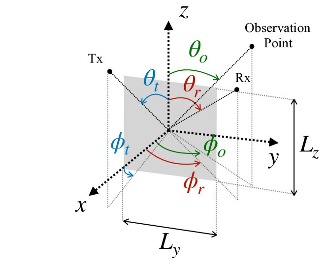
Figure 1: Illustration of the IRS geometry under consideration.

II Electromagnetics-Based Channel Model

Consider a holographic IRS of size $L_{y}\times L_{z}$, where $L_{y}$ and $L_{z}$ denote the dimensions along the $y$ and $z$ directions, respectively. The coordinate system is placed at the center of the IRS, as shown in Fig. 1. Thus, the IRS is represented by the planar surface $\mathcal{S}=\{(y,z):|y|\leq L_{y}/2,|z|\leq L_{z}/2\}$. In the sequel, we focus on the Fresnel zone of the IRS, which refers to all distances $r$ satisfying [16]

$$0.62\sqrt{L_{\max}^{3}/\lambda}<r\leq 2L^{2}_{\max}/\lambda,$$ (1)

where $L_{\max}=\max(L_{y},L_{z})$ denotes the maximum dimension of the IRS, and $\lambda$ is the carrier wavelength.

II-A Spherical Wavefront

Consider an infinitesimal dipole antenna emitting a spherical wave; the dipole is placed parallel to the IRS. The exact position of the transmit antenna is described by the tuple $(x_{t},y_{t},z_{t})=(r_{t}\cos\phi_{t}\sin\theta_{t},r_{t}\sin\phi_{t}\sin\theta_{t},r_{t}\cos\theta_{t})$, where $r_{t}$ is the radial distance, whilst $\phi_{t}$ and $\theta_{t}$ are the azimuth and polar angles of arrival, respectively. The electric field (E-field) of the spherical wave impinging on the $(y,z)$th point of the IRS can be expressed as [16]

$$\mathbf{E}_{i}=E_{\theta}\mathbf{e}_{\theta}=j\sqrt{\frac{\eta P_{t}G_{t}}{4\pi}}\frac{e^{-jkr_{t}(y,z)}}{r_{t}(y,z)}\mathbf{e}_{\theta},$$ (2)

where $\eta$ is the wave impedance, $k=2\pi/\lambda$ is the wavenumber, $P_{t}$ is the transmit power, $G_{t}$ is the gain of the transmit antenna, and

$$r_{t}(y,z)\triangleq\sqrt{x_{t}^{2}+(y_{t}-y)^{2}+(z_{t}-z)^{2}}$$

$$=r_{t}\sqrt{1+\frac{y^{2}}{r_{t}^{2}}-\frac{2\sin\phi_{t}\sin\theta_{t}y}{r_{t}}+\frac{z^{2}}{r_{t}^{2}}-\frac{2\cos\theta_{t}z}{r_{t}}}$$ (3)

is the respective distance. Note that (2) holds for all distances $r_{t}(y,z)\gg\lambda$, where the radial and azimuthal components $E_{r}$ and $E_{\phi}$ of the E-field are approximately zero. From Maxwell’s equations, the magnetic field is specified as

$$\mathbf{H}_{i}=\frac{j}{\eta k}\nabla\times \mathbf{E}_{i}=\frac{j}{\eta k}\frac{1}{r}\frac{\partial(rE_{\theta})}{\partial r}\mathbf{e}_{\phi}$$

$$=\frac{j}{\eta}\sqrt{\frac{\eta P_{t}G_{t}}{4\pi}}\frac{e^{-jkr_{t}(y,z)}}{r_{t}(y,z)}\mathbf{e}_{\phi}=H_{\phi}\mathbf{e}_{\phi},$$ (4)

where $r=r_{t}(y,z)$ in the partial derivative for notational convenience. Owing to the small physical size of THz IRSs, the amplitude variation $1/r_{t}(y,z)$ across $\mathcal{S}$ is marginal [13]; for example, an electrically large IRS of size $200\lambda\times 200\lambda$ occupies only $20\times 20$ cm² at $f=300$ GHz. On the contrary, the phase variation $kr_{t}(y,z)$ is significant and cannot be ignored. In light of these observations, we henceforth consider

$$\frac{e^{-jkr_{t}(y,z)}}{r_{t}(y,z)}\approx\frac{e^{-jk(r_{t}+\tilde{r}_{t}(y,z))}}{r_{t}},$$ (5)

where $r_{t}(y,z)\approx r_{t}+\tilde{r}_{t}(y,z)$, with

$$\tilde{r}_{t}(y,z)= \frac{y^{2}(1-\sin^{2}\phi_{t}\sin^{2}\theta_{t})}{2r_{t}}-y\sin\phi_{t}\sin\theta_{t}$$

$$+\frac{z^{2}\sin^{2}\theta_{t}}{2r_{t}}-z\cos\theta_{t},$$ (6)

which follows from the second-order Taylor approximation $(1+x)^{\alpha}\approx 1+\alpha x+\frac{1}{2}\alpha(\alpha-1)x^{2}$ of (II-A).

II-B Scattered Field in the Fresnel Zone

According to the surface equivalence principle, the obstacle-free equivalent problem involves an electric current density $\mathbf{J}(y,z)$ (measured in A/m²) and a magnetic current density $\mathbf{M}(y,z)$ (measured in V/m²) on $\mathcal{S}$, which satisfy the boundary conditions [17, Ch. 7]

$$\hat{\mathbf{n}}\times\mathbf{H}|_{x=0} =\mathbf{J}(y,z),$$ (7)

$$\hat{\mathbf{n}}\times\mathbf{E}|_{x=0} =\mathbf{M}(y,z)=0,$$ (8)

where $\mathbf{E}=\mathbf{E}_{i}+\mathbf{E}_{s}$ and $\mathbf{H}=\mathbf{H}_{i}+\mathbf{H}_{s}$ are the total electric and magnetic fields, respectively, $\mathbf{E}_{s}$ and $\mathbf{H}_{s}$ are the corresponding scattered fields, and $\hat{\mathbf{n}}=\mathbf{e}_{x}$ is the normal vector of $\mathcal{S}$. Assuming that $\mathcal{S}$ is an infinite PEC, it can be replaced by a virtual source with $\hat{\mathbf{n}}\times\mathbf{H}_{s}=\hat{\mathbf{n}}\times\mathbf{H}_{i}$, hence yielding $\mathbf{J}(y,z)=2\hat{\mathbf{n}}\times\mathbf{H}_{i}|_{x=0}$. Note that the actual IRS exhibits a surface impedance, which can change the phase of the surface current density $\mathbf{J}(y,z)$. Thus, we model that property as $\mathbf{J}(y,z)=(2\hat{\mathbf{n}}\times\mathbf{H}_{i}|_{x=0})e^{j\varphi(y,z)}$ [8],[9]. The phase shift profile $\varphi(y,z)$ is nonlinear due to the spherical wavefront of the incident wave. To this end, it is decomposed as

$$\varphi(y,z)=k\left(C_{1}y^{2}+C_{2}y+C_{3}z^{2}+C_{4}z\right),$$ (9)

where $C_{1}$, $C_{2}$, $C_{3}$, and $C_{4}$ are properly selected constants.

Let $(x_{r},y_{r},z_{r})=(r_{r}\cos\phi_{r}\sin\theta_{r},r_{r}\sin\phi_{r}\sin\theta_{r},r_{r}\cos\theta_{r})$ be the receiver location, where $r_{r}$ is the radial distance, while $\phi_{t}$ and $\theta_{t}$ denote the azimuth and polar angles of departure, respectively. Next, the scattered E-field at the receiver is analytically determined using the auxiliary vector potential

$$\mathbf{A}(x_{r},y_{r}, z_{r})\triangleq\frac{\mu}{4\pi}\int\!\!\!\int_{\mathcal{S}}\mathbf{J}(y,z)\frac{e^{-jkr_{r}(y,z)}}{r_{r}(y,z)}dydz$$

$$\overset{(a)}{\approx}\frac{\mu e^{-jkr_{r}}}{4\pi r_{r}}\int\!\!\!\int_{\mathcal{S}}\mathbf{J}(y,z)e^{-jk\tilde{r}_{r}(y,z)}dydz$$

$$=\frac{\mu e^{-jkr_{r}}}{4\pi r_{r}}(\tilde{A}_{r}\mathbf{e}_{r}+\tilde{A}_{\theta}\mathbf{e}_{\theta}+\tilde{A}_{\phi}\mathbf{e}_{\phi}),$$ (10)

where $\mu$ is the magnetic permeability of the propagation medium, $(a)$ follows from the Fresnel approximation of the distance $r_{r}(y,z)\approx r_{r}+\tilde{r}_{r}(y,z)$, and

$$\tilde{A}_{r}\! =\!\int\!\!\!\!\int_{\mathcal{S}}(J_{y}\sin\theta_{r}\sin\phi_{r}+J_{z}\cos\theta_{r})e^{-jk\tilde{r}_{r}(y,z)}dydz,$$ (11)

$$\tilde{A}_{\theta}\! =\!\int\!\!\!\!\int_{\mathcal{S}}(J_{y}\cos\theta_{r}\sin\phi_{r}-J_{z}\sin\theta_{r})e^{-jk\tilde{r}_{r}(y,z)}dydz,$$ (12)

$$\tilde{A}_{\phi}\! =\!\int\!\!\!\!\int_{\mathcal{S}}J_{y}\cos\phi_{r}e^{-jk\tilde{r}_{r}(y,z)}dydz.$$ (13)

Using the radiation equations for any receive distance $r_{r}\gg\lambda$, we finally have [17, Eq. (6.122)]

$$\mathbf{E}_{s}=-\eta\frac{jke^{-jkr_{r}}}{4\pi r_{r}}(\tilde{A}_{\theta}\mathbf{e}_{\theta}+\tilde{A}_{\phi}\mathbf{e}_{\phi}).$$ (14)

Proposition 1.

The scattered E-field at the receive position $(r_{r}\cos\phi_{r}\sin\theta_{r},r_{r}\sin\phi_{r}\sin\theta_{r},r_{r}\cos\theta_{r})$, when the IRS is illuminated by a spherical wave originated from $(r_{t}\cos\phi_{t}\sin\theta_{t},r_{t}\sin\phi_{t}\sin\theta_{t},r_{t}\cos\theta_{t})$, is given by

$$\mathbf{E}_{s} =-\frac{L_{y}L_{z}}{\lambda}\frac{|E_{i}|e^{-jk(r_{t}+r_{r})}}{r_{r}}\cos\phi_{t}\sin\theta_{r}S_{yz}\mathbf{e}_{\theta},$$ (15)

where $|E_{i}|=\sqrt{\frac{\eta P_{t}G_{t}}{4\pi r^{2}_{t}}}$ is the magnitude of the incident field, and $S_{yz}\in[0,1]$ is the normalized space factor of the IRS specified by (1) at the bottom of the next page for

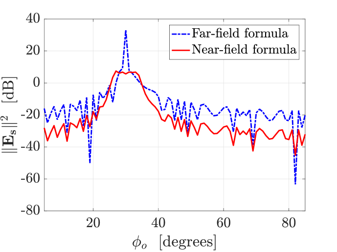
(a) $r_{r}=2$ m and $r_{o}=8$ m

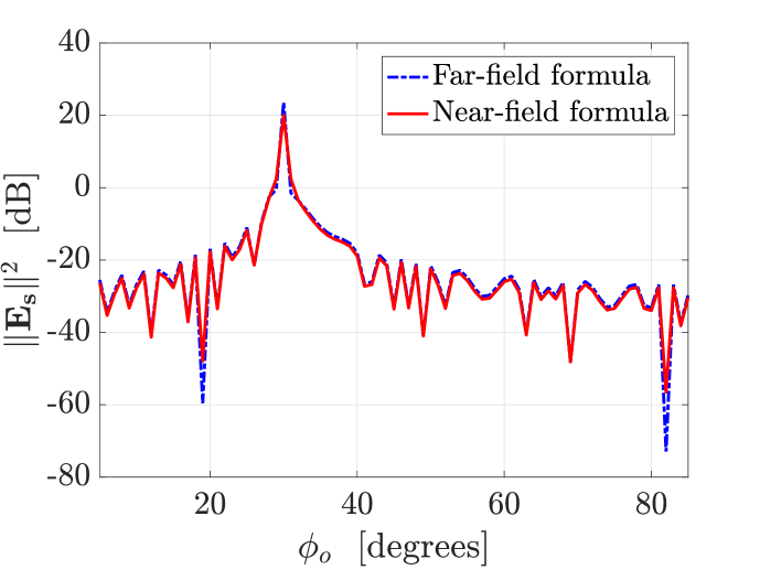
(b) $r_{r}=6$ m and $r_{o}=8$ m

Figure 2: Squared magnitude of the scattered E-field versus observation angle $\phi_{o}$; $|E_{i}|=1$, $L_{y}=L_{z}=200\lambda$, $f=300$ GHz, $\phi_{t}=36\degree$, $(\theta_{r},\phi_{r})=(45\degree,30\degree)$, and $(\theta_{o},\phi_{o})=(45\degree,\phi_{o})$.

$$S_{yz}=\frac{\pi}{4jkL_{y}L_{z}\sqrt{a_{y}a_{z}}}\left[\text{erf}\left(\sqrt{jka_{y}}\left(\frac{L_{y}}{2}-\frac{b_{y}}{2a_{y}}\right)\right)-\text{erf}\left(\sqrt{jka_{y}}\left(-\frac{L_{y}}{2}-\frac{b_{y}}{2a_{y}}\right)\right)\right]$$

$$\quad\quad\quad\quad\quad\times\left[\text{erf}\left(\sqrt{jka_{z}}\left(\frac{L_{z}}{2}-\frac{b_{z}}{2a_{z}}\right)\right)-\text{erf}\left(\sqrt{jka_{z}}\left(-\frac{L_{z}}{2}-\frac{b_{z}}{2a_{z}}\right)\right)\right].$$ (16)

$$a_{y} =\frac{(1-\sin^{2}\phi_{t}\sin^{2}\theta_{t})}{2r_{t}}+\frac{(1-\sin^{2}\phi_{r}\sin^{2}\theta_{r})}{2r_{r}}-C_{1},$$

$$b_{y} =\sin\phi_{t}\sin\theta_{t}+\sin\phi_{r}\sin\theta_{r}+C_{2},$$ (17)

$$a_{z} =\frac{\sin^{2}\theta_{t}}{2r_{t}}+\frac{\sin^{2}\theta_{r}}{2r_{r}}-C_{3},$$

$$b_{z} =\cos\theta_{t}+\cos\theta_{r}+C_{4}.$$ (18)

Proof.

See Appendix. ∎

Remark 1.

In the far-field, the parallel-ray approximations

$$\tilde{r}_{t}(y,z) \approx-y\sin\phi_{t}\sin\theta_{t}-z\cos\theta_{t},$$ (19)

$$\tilde{r}_{r}(y,z) \approx-y\sin\phi_{r}\sin\theta_{r}-z\cos\theta_{r}$$ (20)

are employed. Then, $a_{y}=a_{z}=0$, and the space factor reduces to [17]

$$S_{yz}=\frac{\int_{-L_{y}/2}^{L_{y}/2}\int_{-L_{z}/2}^{L_{z}/2}e^{jk(b_{y}y+b_{z}z)}dydz}{L_{y}L_{z}}=\emph{sinc}(Y)\emph{sinc}(Z),$$ (21)

where $Y\triangleq kL_{y}b_{y}/2$ and $Z\triangleq kL_{z}b_{z}/2$.

From Proposition 1, the squared magnitude of the scattered E-field is calculated as

$$\|\mathbf{E}_{s}\|^{2} =\left(\frac{L_{y}L_{z}}{\lambda}\right)^{2}\frac{|E_{i}|^{2}}{r_{r}^{2}}\cos^{2}\phi_{t}\sin^{2}\theta_{r}|S_{yz}|^{2},$$ (22)

where $|S_{yz}|^{2}$ is the normalized beampattern of the IRS.

II-C End-to-End Signal Model

We now introduce the signal model of a holographic IRS-assisted THz system, where the Tx and Rx are equipped with a single antenna each. First, recall the relation between the magnitude of the incident wave $|E_{i}|$ and the transmit power $P_{t}$, which is $|E_{i}|^{2}/\eta=G_{t}P_{t}/(4\pi r^{2}_{t})$ [16]. Hence, the power density (W/m²) of the scattered field is

$$S_{s}=\frac{\|\mathbf{E}_{s}\|^{2}}{\eta}=\left(\frac{L_{y}L_{z}}{\lambda}\right)^{2}\frac{P_{t}G_{t}}{4\pi r^{2}_{t}r_{r}^{2}}\cos^{2}\phi_{t}\sin^{2}\theta_{r}|S_{yz}|^{2}.$$ (23)

Considering the Rx antenna aperture $A_{r}=G_{r}\lambda^{2}/(4\pi)$ yields the received power $P_{r}=S_{s}A_{r}$. Lastly, taking into account the molecular absorption loss at THz frequencies results in the path loss of the Tx-IRS-Rx link

$$\overline{\text{PL}} =G_{t}G_{r}\left(\frac{L_{y}L_{z}}{4\pi}\right)^{2}\frac{\cos^{2}\phi_{t}\sin^{2}\theta_{r}}{r_{t}^{2}r_{r}^{2}}e^{-\kappa_{\text{abs}}(f)(r_{t}+r_{r})}|S_{yz}|^{2}$$

$$=\text{PL}|S_{yz}|^{2},$$ (24)

where $\kappa_{\text{abs}}(f)$ denotes the molecular absorption coefficient at the carrier frequency $f$. From (II-C), it is evident that the path loss of an IRS-assisted link follows the plate scattering paradigm. Combining (15) and (II-C), the baseband signal at the Rx is written as

$$y=\left(\sqrt{\text{PL}}e^{-jk(r_{r}+r_{t})}S_{yz}+\sqrt{\text{PL}_{d}}e^{-jkr_{d}}\right)s+\tilde{n},$$ (25)

where $s\sim\mathcal{CN}(0,P_{t})$ is the transmitted data symbol, $P_{t}$ is the average power per data symbol, $r_{d}$ is the distance between the Tx and Rx, $\text{PL}_{d}=G_{t}G_{r}\lambda^{2}/(4\pi r_{d})^{2}e^{-\kappa_{\text{abs}(f)}r_{d}}$ is the path loss of the direct Tx-Rx channel, and $\tilde{n}\sim\mathcal{CN}(0,\sigma^{2})$ is the additive noise.

III Discussion

In this section, we discuss in detail the near-field channel model introduced in Section II.

III-A Near-Field versus Far-Field Response

Consider the phase profile (9) with

$$C_{1} =\frac{1-\sin^{2}\phi_{t}\sin^{2}\theta_{t}}{2r_{t}}+\frac{1-\sin^{2}\phi_{o}\sin^{2}\theta_{o}}{2r_{o}},$$ (26)

$$C_{2} =-\sin\phi_{t}\sin\theta_{t}-\sin\phi_{o}\sin\theta_{o},$$ (27)

$$C_{3} =\frac{\sin^{2}\theta_{t}}{2r_{t}}+\frac{\sin^{2}\theta_{o}}{2r_{o}},$$ (28)

$$C_{4} =-\cos\theta_{t}-\cos\theta_{o},$$ (29)

where $(r_{o}\cos\phi_{o}\sin\theta_{o},r_{o}\sin\phi_{o}\sin\theta_{o},r_{o}\cos\theta_{o})$ is an arbitrary observation position, with $r_{o}$, $\phi_{o}$, and $\theta_{o}$ denoting the corresponding radial distance, azimuth angle, and polar angle, respectively. Then, the parameters of the beampattern $|S_{yz}|^{2}$ are

$$a_{y} =\frac{1-\sin^{2}\phi_{r}\sin^{2}\theta_{r}}{2r_{r}}-\frac{1-\sin^{2}\phi_{o}\sin^{2}\theta_{o}}{2r_{o}},$$ (30)

$$b_{y} =\sin\phi_{r}\sin\theta_{r}-\sin\phi_{o}\sin\theta_{o},$$ (31)

$$a_{z} =\frac{\sin^{2}\theta_{r}}{2r_{r}}-\frac{\sin^{2}\theta_{o}}{2r_{o}},$$ (32)

$$b_{z} =\cos\theta_{r}-\cos\theta_{o}.$$ (33)

We now plot the squared magnitude of the scattered E-field for the considered $\varphi(y,z)$. From Fig. 2, we first observe that the peak value is at $\phi_{o}=\phi_{r}=30\degree$, as expected. From Fig. 2(2(a)), however, we see a mismatch between the near and far scattered fields of a large IRS. This discrepancy is due to the spherical wavefront of the incident wave, which makes the beampattern $|S_{xy}|^{2}$ depend on the angles of arrival/departure as well as the distances between the IRS, the Rx, and the observation point. This unique feature manifests only in the near-field [18]. It is finally worth stressing that the near-field space factor in (1) coincides with its far-field counterpart (21) for either an electrically small IRS or relatively large distances $r_{r}$ and $r_{o}$, i.e., Fig. 2(2(b)).

III-B Discrete IRS

It might be difficult to implement a holographic IRS in practice. Therefore, a contiguous IRS of size $L_{y}\times L_{z}$ can be approximated by a planar array of $N_{y}=L_{y}/\tilde{L}_{y}$ and $N_{z}=L_{z}/\tilde{L}_{z}$ reflecting elements, each of size $\tilde{L}_{y}\times\tilde{L}_{z}$; the inter-element spacing is negligible, and hence is ignored. Then, (22) is recast as

$$\|\mathbf{E}_{s}\|^{2}=N^{2}_{y}N^{2}_{z}\left(\frac{\tilde{L}_{y}\tilde{L}_{z}}{\lambda}\right)^{2}\frac{|E_{i}|^{2}}{r_{o}^{2}}\cos^{2}\phi_{t}\sin^{2}\theta_{r}|S_{yz}|^{2},$$ (34)

where

$$S_{yz} =\frac{\sum_{n=-\frac{N_{y}}{2}}^{\frac{N_{y}}{2}-1}e^{-jk\left((n\tilde{L}_{y})^{2}a_{y}-n\tilde{L}_{y}b_{y}\right)}}{N_{y}}$$

$$\times\frac{\sum_{m=-\frac{N_{z}}{2}}^{\frac{N_{z}}{2}-1}e^{-jk\left((m\tilde{L}_{z})^{2}a_{z}-m\tilde{L}_{z}b_{z}\right)}}{N_{z}},$$ (35)

which follows from (Appendix) in the appendix for $y=n\tilde{L}_{y}$, $z=m\tilde{L}_{z}$, $L_{y}=N_{y}\tilde{L}_{y}$, $L_{z}=N_{z}\tilde{L}_{z}$, $dy=\tilde{L}_{y}$, and $dz=\tilde{L}_{z}$. Likewise, the reflection coefficient of the $(n,m)$th IRS element is defined as $e^{j\varphi_{n,m}}$, where $\varphi_{n,m}\triangleq\varphi(n\tilde{L}_{y},m\tilde{L}_{z})$. For a discrete IRS, when the observation direction coincides with that of the Rx, $a_{y}=b_{y}=a_{z}=b_{z}=0$, $S_{yz}=1$, and a power gain of $(N_{y}N_{z})^{2}$ is attained over the Tx-IRS-Rx link.

(a) Small IRS

(b) Large IRS

Figure 3: Normalized beampattern of holographic IRS and discrete IRS versus observation angle $\phi_{o}$; $\tilde{L}_{y}=\tilde{L}_{z}=\lambda$, $(r_{r},\theta_{r},\phi_{r})=(2,45\degree,45\degree)$, $(r_{o},\theta_{o},\phi_{o})=(8,\theta_{o},45\degree)$, and $f=300$ GHz.

III-C Beamfocusing Capabilities

With proper design of the phase profile $\varphi(y,z)$, we can cancel out the incident phase and focus the beam into the Rx point $(r_{r},\theta_{r},\phi_{r})$. As previously shown, the peak value of $|S_{yz}|^{2}$ occurs at $(r_{o},\theta_{o},\phi_{o})=(r_{r},\theta_{r},\phi_{r})$. From Fig. 3(3(a)) and Fig. 3(3(b)), we first observe the excellent match between a holographic IRS and its discrete counterpart with a negligible inter-element spacing. This implies that we can properly discretize the holographic IRS without sacrificing its extremely high spatial resolution. Consequently, (1) and (III-B) can be used interchangeably. We further see that the electrically large IRS can discriminate two points with the same angular direction $(\theta_{o},\phi_{o})=(\theta_{r},\phi_{r})$ but with different distances $r_{o}\neq r_{r}$; asymptotically, we have $|S_{yz}|^{2}\to 0$ as $L_{y}L_{z}\to\infty$. The beamfocusing capability can be exploited in multi-user transmissions to suppress interference with an unprecedented way. For example, consider an uplink scenario where two users, user $1$ and user $2$, simultaneously transmit. Their positions from the IRS are $(r_{1},\theta_{1},\phi_{1})$ and $(r_{2},\theta_{2},\phi_{2})$, with $(\theta_{1},\phi_{1})=(\theta_{2},\phi_{2})$ and $r_{1}\neq r_{2}$. In the far-field, $|S_{yz}|^{2}=1$, and hence we will have strong inter-user interference at the Rx. Conversely, in the near-field, $|S_{yz}|^{2}<1$ and the inter-user interference becomes small at the Rx.

III-D Scattering versus Antenna-Based Path Loss Models

Some works in the literature (e.g., [11]) treat an IRS element as a standard antenna that re-radiates the impinging wave. In this case, the path loss is calculated as

$$\text{PL}^{\prime}=G_{t}G_{r}\left(\frac{\lambda}{4\pi}\right)^{4}\frac{G_{e}(\theta_{t})G_{e}(\theta_{r})}{r^{2}_{t}r^{2}_{r}}e^{-\kappa_{\text{abs}}(f)(r_{t}+r_{r})},$$ (36)

where $G_{e}(\cdot)$ is the radiation pattern of each IRS element. For a sub-wavelength IRS element, it holds that $|S_{yz}|^{2}\approx 1$, and $\text{PL}=G_{t}G_{r}\left(\frac{L_{y}L_{z}}{4\pi}\right)^{2}\frac{\cos^{2}\phi_{t}\sin^{2}\theta_{r}}{r_{t}^{2}r_{r}^{2}}e^{-\kappa_{\text{abs}}(f)(r_{t}+r_{r})}\neq\text{PL}^{\prime}$, as shown in Fig. 4. Consequently, simplistic path loss models may not always capture the unique features of IRS-aided propagation.

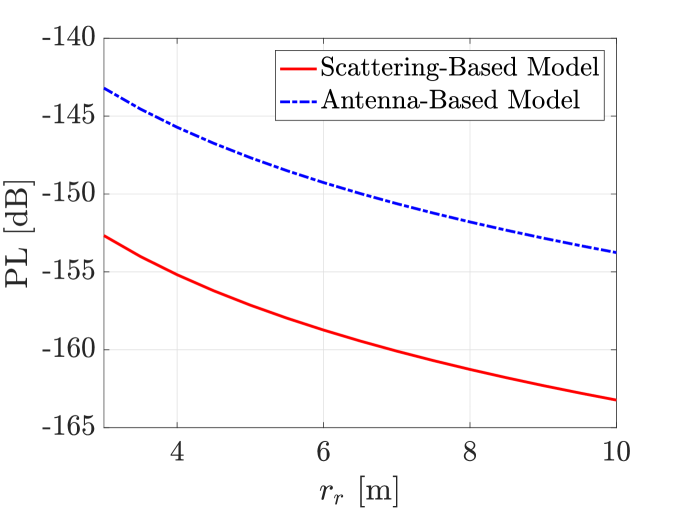
Figure 4: In the antenna-based model [11], $G_{e}(\theta)=\gamma\cos^{2q}\theta$, with $\gamma=\pi$ and $q=0.285$. The other parameters are: $f=300$ GHz, $L_{y}=L_{z}=\lambda/2$, $r_{t}=2$ m, $(\theta_{t},\phi_{t})=(60\degree,90\degree)$, $(\theta_{r},\phi_{r})=(45\degree,90\degree)$, $G_{t}=20$ dBi, $G_{r}=0$ dBi, and $\kappa_{\text{abs}}(f)=0.0033$ m^-1.

IV Conclusions

We have studied, for the first time, the near-field response of holographic IRSs operating at the THz frequency band. To have a physics-consistent channel model, we leveraged EM theory and derived a novel closed-form expression for the scattered field. Unlike existing works, our model accounts for arbitrary incident and reflection angles. Capitalizing on our analysis, we then compared the near-field response with its far-field counterpart and revealed a significant discrepancy, which makes the use of the former necessary for electrically large IRSs. We finally discussed the beamfocusing property, which manifests on the near-field regime, and highlighted its potential in multi-user transmissions and interference suppression. For future work, it would be interesting to study the coupling effects in ultra-dense discrete IRSs and their connection with super-directive antenna arrays. Moreover, it would be interesting to derive a circuit theory-based model for the power consumption of THz IRSs.

Appendix

The magnetic field in (II-A) is written in Cartesian coordinates as

$$\mathbf{H}_{i}=-H_{\phi}\sin\phi_{t}\mathbf{e}_{x}+H_{\phi}\cos\phi_{t}\mathbf{e}_{y}.$$ (37)

The current density induced on the IRS is

$$\mathbf{J}(y,z)=(2\mathbf{e}_{x}\times\mathbf{H}_{i}|_{x=0})e^{j\varphi(y,z)}$$

$$=2H_{\phi}\cos\phi_{t}e^{j\varphi(y,z)}\mathbf{e}_{z}$$

$$=\frac{2j}{\eta}\sqrt{\frac{\eta P_{t}G_{t}}{4\pi}}\frac{e^{-jkr_{t}}}{r_{t}}e^{-jk\tilde{r}_{t}(y,z)}\cos\phi_{t}e^{j\varphi(y,z)}\mathbf{e}_{z}$$

$$=\frac{2j}{\eta}E_{i}e^{-jk\tilde{r}_{t}(y,z)}\cos\phi_{t}e^{j\varphi(y,z)}\mathbf{e}_{z}$$

$$=J_{z}e^{j\varphi(y,z)}\mathbf{e}_{z},$$ (38)

where $E_{i}=\sqrt{\frac{\eta P_{t}G_{t}}{4\pi}}\frac{e^{-jkr_{t}}}{r_{t}}$. Then, (12) and (13) give

$$\tilde{A}_{\theta}=-jL_{y}L_{z}\frac{2E_{i}}{\eta}\cos\phi_{t}\sin\theta_{r}S_{yz},$$ (39)

$$\tilde{A}_{\phi}=0,$$ (40)

where

$$S_{yz} =\frac{\int\!\!\int_{\mathcal{S}}e^{-jk(\tilde{r}_{t}(y,z)+\tilde{r}_{r}(y,z)-\varphi(y,z)/k)}ds}{L_{y}L_{z}}$$

$$=\frac{\int_{-L_{y}/2}^{L_{y}/2}\int_{-L_{z}/2}^{L_{z}/2}e^{-jk(a_{y}y^{2}-b_{y}y+a_{z}z^{2}-b_{z}z)}dydz}{L_{y}L_{z}},$$ (41)

with

$$a_{y} =\frac{(1-\sin^{2}\phi_{t}\sin^{2}\theta_{t})}{2r_{t}}+\frac{(1-\sin^{2}\phi_{r}\sin^{2}\theta_{r})}{2r_{r}}-C_{1},$$

$$b_{y} =\sin\phi_{t}\sin\theta_{t}+\sin\phi_{r}\sin\theta_{r}+C_{2},$$ (42)

$$a_{z} =\frac{\sin^{2}\theta_{t}}{2r_{t}}+\frac{\sin^{2}\theta_{r}}{2r_{r}}-C_{3},$$ (43)

$$b_{z} =\cos\theta_{t}+\cos\theta_{r}+C_{4}.$$ (44)

We now use the identity

$$\int e^{-jk(ay^{2}-by)}dy=\frac{\sqrt{\pi}}{2\sqrt{jka}}\text{erf}\left(\sqrt{jka}\left(y-\frac{b}{2a}\right)\right),$$ (45)

which follows from the definition of the error function, some algebrain manipulations, and a change of variables. Using (45), the expression (1) for $S_{yz}$ is derived. The scattered E-field is finally given by

$$\mathbf{E}_{s}=-\eta\frac{jke^{-kjr_{r}}}{4\pi r_{r}}(\tilde{A}_{\theta}\mathbf{e}_{\theta}+\tilde{A}_{\phi}\mathbf{e}_{\phi})$$

$$=\frac{j^{2}L_{y}L_{z}kE_{i}e^{-kj(r_{t}+r_{r})}}{2\pi r_{r}}\cos\phi_{t}\sin\theta_{r}S_{yz}\mathbf{e}_{\theta}$$

$$=-\frac{L_{y}L_{z}}{\lambda}\frac{|E_{i}|e^{-kj(r_{t}+r_{r})}}{r_{r}}\cos\phi_{t}\sin\theta_{r}S_{yz}\mathbf{e}_{\theta},$$ (46)

which completes the proof.

References

• [1] T. S. Rappaport et al., “Wireless communications and applications above 100 GHz: Opportunities and challenges for 6G and beyond,” IEEE Access, vol. 7, pp. 78729-78757, 2019.
• [2] J. Zhang et al., “Prospective multiple antenna technologies for beyond 5G,” IEEE J. Sel. Areas Commun., vol. 38, no. 8, pp. 1637–1660, Aug. 2020.
• [3] K. Dovelos, M. Matthaiou, H. Q. Ngo, and B. Bellalta, “Channel estimation and hybrid combining for wideband terahertz massive MIMO systems,” IEEE J. Sel. Areas Commun., vol. 39, no. 6, pp. 1604-1620, Jun. 2021.
• [4] M. D. Renzo et al., “Smart radio environments empowered by reconfigurable intelligent surfaces: How it works, state of research, and road ahead,” IEEE J. Sel. Areas Commun., vol. 38, no. 11, pp. 2450–2525, Nov. 2020.
• [5] M. Di Renzo et al., “Reconfigurable intelligent surfaces vs. relaying: Differences, similarities, and performance comparison,” IEEE Open J. Commun. Soc., vol. 1, pp. 798-807, 2020.
• [6] K. Ntontin et al., “Reconfigurable intelligent surface optimal placement in millimeter-wave networks,” Open J. Commun. Soc., vol. 2, pp. 704-718, Mar. 2021.
• [7] A.-A. A. Boulogeorgos and A. Alexiou, “Coverage analysis of reconfigurable intelligent surface assisted THz wireless systems,” IEEE Open J. Veh. Technol., vol. 2, pp. 94-110, Jan. 2021.
• [8] Ö. Özdogan, E. Björnson, and E. G. Larsson, “Intelligent reflecting surfaces: Physics, propagation, and pathloss modeling,” IEEE Wireless Commun. Lett., vol. 9, no. 5, pp. 581-585, May 2020.
• [9] M. Najafi, V. Jamali, R. Schober, and H. V. Poor, “Physics-based modeling and scalable optimization of large intelligent reflecting surfaces,” IEEE Trans. Commun., vol. 69, no. 4, pp. 2673-2691, Apr. 2021.
• [10] C. Huang et al., “Holographic MIMO surfaces for 6G wireless networks: Opportunities, challenges, and trends,” IEEE Wireless Commun., vol. 27, no. 5, pp. 118-125, Oct. 2020.
• [11] S. W. Ellingson, “Path loss in reconfigurable intelligent surface-enabled channels,” arXiv preprint arXiv:1912.06759, 2019.
• [12] W. Tang et al., “Wireless communications with reconfigurable intelligent surface: Path loss modeling and experimental measurement,” IEEE Trans. Wireless Commun., vol. 20, no. 1, pp. 421-439, Jan. 2021.
• [13] K. Dovelos, S. D. Assimonis, H. Q. Ngo, B. Bellalta, and M. Matthaiou, “Intelligent reflecting surfaces at terahertz bands: Channel modeling and analysis,” in Proc. IEEE ICC, Jun. 2021, pp. 1-6.
• [14] E. Björnson and L. Sanguinetti, “Power scaling laws and near-field behaviors of massive MIMO and intelligent reflecting surfaces,” IEEE Open J. Commun. Soc., vol. 1, pp. 1306–1324, 2020.
• [15] Z. Wan, Z. Gao, M. Di Renzo, and M.-S. Alouini, “Terahertz massive MIMO with holographic reconfigurable intelligent surfaces,” IEEE Trans. Commun., Mar. 2021.
• [16] C. A. Balanis, Antenna Theory: Analysis and Design, John Wiley & Sons, 2012.
• [17] C. A. Balanis, Advanced Engineering Electromagnetics, 2nd ed. John Wiley & Sons, 2012.
• [18] O. Yurduseven, S. D. Assimonis, and M. Matthaiou, “Intelligent reflecting surfaces with spatial modulation: An electromagnetic perspective,” IEEE Open J. Commun. Soc., vol. 1, pp. 1256–1266, Sep. 2020.
• [19] A. V. Osipov and S. A. Tretyakov, Modern Electromagnetic Scattering Theory with Applications, John Wiley, 2017.
• [20] E. Björnson, Ö. Özdogan, and E. G. Larsson, “Reconfigurable intelligent surfaces: Three myths and two critical questions,” IEEE Commun. Mag., vol. 58, no. 12, pp. 90-96, Dec. 2020.