Shapes of Non-symmetric Capillary Bridges

Abstract

Here we study the shapes of droplets captured between chemically distinct parallel plates. This work is a preliminary step toward characterizing the influence of second-phase bridging between biomolecular surfaces on their solution contacts, i.e., capillary attraction or repulsion. We obtain a simple, variable-separated quadrature formula for the bridge shape. The technical complication of double-ended boundary conditions on the shapes of non-symmetric bridges is addressed by studying waists in the bridge shape, i.e., points where the bridge silhouette has zero derivative. Waists are always expected with symmetric bridges, but waist-points can serve to characterize shape segments in general cases. We study how waist possibilities depend on the physical input to these problems, noting that these formulae change with the sign of the inside-outside pressure difference of the bridge. These results permit a variety of different interesting shapes, and the development below is accompanied by several examples.

I Introduction

Here we study the shapes of non-symmetric capillary bridges between planar contacts (FIG. 1), laying a basis for studying the forces that result from the bridging.

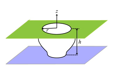
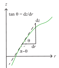
Figure 1: (above) Non-symmetric capillary bridge studied here, and (below) angles associated with a general droplet shape.

The recent measurements of Cremaldi, et al.,¹ provide a specific motivation for this work. A helpful monograph² sketches adhesion due to symmetric capillary bridges, albeit with aspect ratio (width/length $\approx$ 10³) vastly different than is considered below. Additionally, that sketch² does not specifically consider non-symmetric cases surveyed by Cremaldi, et al.¹ A specific description applicable to non-symmetric cases is apparently unavailable,³ and, thus, is warranted here.

A background aspect of our curiosity in these problems is the possibility of evaporative bridging between ideal hydrophobic surfaces, influencing the solution contacts between biomolecules.^{4; 5; 6; 7; 8; 9; 10} Assessment of critical evaporative lengths in standard aqueous circumstances on the basis of explicit thermophysical properties⁸ sets those lengths near 1 $\mu$m. Though we do not specifically discuss that topic further here, our analytical development does hinge on identification of the length $\ell=2\gamma/|\Delta p|$, with $\gamma$ the fluid interfacial tension, and $\Delta p$ the pressure difference between inside and outside of the bridge. The experiments that motivate this study considered spans $\lesssim\left(6\mu\mathrm{L}\right)^{1/3}\approx 1.8$ mm.¹

A full development of the essential basics of this problem might be dense in statistical-thermodyamics. We strive for concision in the presentation below but follow² a Grand Ensemble formulation of our problem. We then develop the optimization approach analogous to Hamilton’s Principle of classical mechanics.^{2; 11} That approach avoids more subtle issues of differential geometry related to interfacial forces, and, eventually, should clarify the thermodynamic forces for displacement of the confining plates. Along the way, we support the theoretical development by displaying typical solutions of our formulation.

II Statistical Thermodynamic Formulation

Consider two plates, not necessarily the same, oriented perpendicular to the $z$-axis and separated by a distance $h$ (FIG. 1). A droplet captured between two parallel plates is assumed to be cylindrically symmetric about the $z$-axis. We want to determine the droplet shape (FIG. 2) in advance of analyses of the forces involved. We study

$$\Delta\Omega\left[r\right]=-2\pi\Delta p\int\limits_{-h/2}^{h/2}\left(r^{2}/2\right)\mathrm{d}z\\ +2\pi\gamma\int\limits_{-h/2}^{h/2}r\sqrt{1+\dot{r}{}^{2}}\;\mathrm{d}z\\ +\pi r_{+}{}^{2}\Delta\gamma_{+}+\pi r_{-}{}^{2}\Delta\gamma_{-}~{},$$ (1)

a functional of the droplet radius $r(z)$. Here $\dot{r}=\mathrm{d}r(z)/\mathrm{d}z$ and $r_{\pm}=r(z=\pm h/2)$. $\gamma$ is the tension between the droplet and the external solution. $\Delta\gamma_{+}$ is the inside-outside difference of the surface tensions of the fluids against the plate at $z=+h/2$ (and similarly for $\Delta\gamma_{-}$ with the fluids against the plate at $z=-h/2$); this differencing will be clarified below as we note how this leads to Young’s Law. $\Delta p$ is the traditional Laplace inside-outside pressure difference of the bridge. The usual Grand Ensemble potential for a single-phase uniform fluid solution being $-\Omega=pV$, it is natural that $\Delta\Omega\left[r\right]$ of Eq. (1) has $\Omega$ for the surrounding fluid solution subtracted away; i.e, the pressure-volume term of Eq. (1) evaluates the pressure-inside times the bridge volume, minus the pressure-outside times the same bridge volume. Formally

$$-\Omega=-F+\sum_{\alpha}\mu_{\alpha}n_{\alpha}~{},$$ (2)

with $F$ the Helmholtz free energy. Therefore, the surface-area feature of Eq. (1) can be viewed as an addition of $\gamma A$ contribution to $F$, with $A$ the surface area of contact of the bridge with the external fluid and $\gamma$ is the tension of the fluid-fluid interface.

An alternative perspective on $\Delta\Omega$ (Eq. (1)) is that it is a Lagrangian function for finding a minimum surface area of the bridge satisfying a given value of the bridge volume. Then $\Delta p/\gamma$, which has dimensions of an inverse length, serves as a Lagrange multiplier. We then minimize $\Delta\Omega$ with respect to variations of $r(z)$, targeting a specific value of the droplet volume.

The first-order variation of $\Delta\Omega$ is then

$$\frac{\delta\Delta\Omega}{2\pi}=-\Delta p\int\limits_{-h/2}^{h/2}r\delta r\mathrm{d}z\\ +\gamma\int\limits_{-h/2}^{h/2}\left\{\left(\frac{\dot{r}r}{\sqrt{{1+\dot{r}^{2}}}}\right)\delta\dot{r}+\left(\sqrt{1+\dot{r}^{2}}\right)\delta r\right\}\mathrm{d}z\\ +r_{+}\Delta\gamma_{+}\delta r_{+}+r_{-}\Delta\gamma_{-}\delta r_{-}~{}.$$ (3)

The angle that the shape curve $r(z)$ makes with the plane perpendicular to the $z$ axis (FIG. 1) is

$$\cos^{2}\theta=\frac{\dot{r}{}^{2}}{1+\dot{r}{}^{2}}~{},$$ (4)

and at the contacting surfaces

$$\left(\mp\right)\cos\theta_{\pm}=\frac{\dot{r}_{\pm}}{\sqrt{1+\dot{r}_{\pm}{}^{2}}}~{}.$$ (5)

Depicted in FIG. 1 is the choice of the bottom sign above, where $0<\dot{r}<\infty$. For $\theta_{+}$ we change the choice so that the contact angle at the upper plate is the traditional external angle of the droplet.

The usual integration-by-parts for Eq. (3) gives

$$\frac{\delta\Omega}{2\pi}=\\ \int\limits_{-h/2}^{h/2}\left\{-\gamma\frac{\mathrm{d}}{\mathrm{d}z}\left(\frac{\dot{r}r}{\sqrt{1+\dot{r}^{2}}}\right)+\gamma\sqrt{1+\dot{r}^{2}}-r\Delta p\right\}\delta r\mathrm{d}z\\ +\left(\Delta\gamma_{+}+\frac{\gamma\dot{r}_{+}}{\sqrt{1+\dot{r}_{+}{}^{2}}}\right)r_{+}\delta r_{+}\\ +\left(\Delta\gamma_{-}-\frac{\gamma\dot{r}_{-}}{\sqrt{1+\dot{r}_{-}{}^{2}}}\right)r_{-}\delta r_{-}~{}.$$ (6)

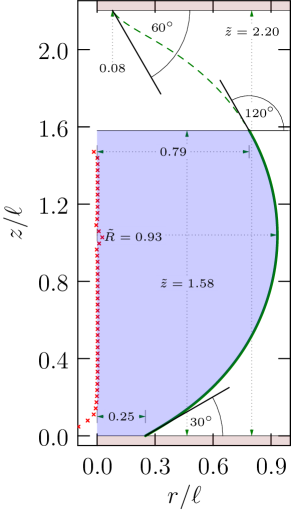
Figure 2: Droplet dimensions using lengths scaled by $\ell=2\gamma/\Delta p$, with $\Delta p>0$. That the pressure is higher inside than outside the droplet is recognized by noting that $\ddot{r}$ is negative at the waist. The separation of variables of Eq. (18) suggests taking $r$ (the horizontal axis) as the independent variable. At the bottom contact $\tilde{r}_{-}=\frac{1}{2}\sin\theta_{-}$ in Eq. (15) with $\theta=30^{\circ}$. The waist has radius $\tilde{R}=\frac{1}{2}\left(1+\cos\theta_{-}\right)\approx 0.93$. The alternative solution of Eq. (15) is $\frac{1}{2}\left(1-\cos\theta_{-}\right)\approx 0.067$, smaller than the radius of the upper contact, $\approx 0.08$. The contact angle $\theta_{+}=60^{\circ}$ together with $\tilde{R}$, Eq. (15) gives $\tilde{r}_{+}\approx 0.79$, confirming the connection between branches above and below the waist. The dashed curve thus extends the solid curve. At each height, the red crosses mark the discrepancies of the Euler-Lagrange Eq. (9) from zero.

With the signs indicated in Eq. (5)

$$\frac{\delta\Delta\Omega}{2\pi}=\\ \int\limits_{-h/2}^{h/2}\left\{-\gamma\frac{\mathrm{d}}{\mathrm{d}z}\left(\frac{\dot{r}r}{\sqrt{1+\dot{r}^{2}}}\right)+\gamma\sqrt{1+\dot{r}^{2}}-r\Delta p\right\}\delta r\mathrm{d}z\\ +\left(\Delta\gamma_{+}-\gamma\cos\theta_{+}\right)r_{+}\delta r_{+}\\ +\left(\Delta\gamma_{-}-\gamma\cos\theta_{-}\right)r_{-}\delta r_{-}~{},$$ (7)

with the exterior angles contacting the upper and lower plates.

The contact terms in Eq. (7) vanish if the contact angles obey the force balance

$$\Delta\gamma_{\pm}=\gamma\cos\theta_{\pm}$$ (8)

of the traditional Young’s Law. This re-inforces the sign choice for Eq. (5). Eq. (8) will provide boundary information for $r(z)$.

From Eq. (7), we require that the kernel

$$-\gamma\frac{\mathrm{d}}{\mathrm{d}z}\left(\frac{\dot{r}r}{\sqrt{1+\dot{r}^{2}}}\right)+\gamma\sqrt{1+\dot{r}^{2}}-r\Delta p=0~{}$$ (9)

vanish identically in $z$. As with Young’s Law, this balances the forces for varying the droplet radius. For the example of a spherical droplet of radius $R$, this force balance implies the traditional Laplace pressure formula, $\Delta p=2\gamma/R$.

The traditional Hamilton’s principle¹¹ analysis of this formulation then yields the usual energy conservation theorem^{2; 11}

$$\frac{\gamma r}{\sqrt{1+\dot{r}{}^{2}}}-r^{2}\Delta p/2=D~{},$$ (10)

with $D$ a constant of integration. $D+r^{2}\Delta p/2$ is non-negative according to Eq. (10). Recognizing that sign, then

$$\gamma r\sin\theta\left(z\right)=D+r^{2}\Delta p/2~{},$$ (11)

with $0\leq\theta\left(z\right)\leq\pi$. The constant $D$ can be eliminated in terms of boundary information, e.g.,

$$\gamma r_{-}\sin\theta_{-}-r_{-}^{2}\Delta p/2=D~{}.$$ (12)

This helpfully correlates $r(z)$ at other places too. For example, we will consider (FIG. 2) intermediate positions where $\dot{r}\left(z\right)=0$ and $\sin\theta\left(z\right)=1$. We call such a position a ‘waist.’ A waist is expected for symmetric cases that we build from here. Denoting the radius of a waist by $R$, then

$$\gamma R=D+R^{2}\Delta p/2~{},$$ (13)

from Eq. (10). This eliminates the integration constant $D$ in favor of $R$ which may be more meaningful.

II.1 $\Delta p>0$

Considering $\Delta p>0$ we can make these relations more transparent by non-dimensionalizing them with the length $\ell=2\gamma/\Delta p$. Then $r=\tilde{r}\ell$ and $R=\tilde{R}\ell$, so

$$\tilde{r}_{-}\left(\tilde{r}_{-}-\sin\theta_{-}\right) = \tilde{R}\left(\tilde{R}-1\right)~{}.$$ (14)

Though this scaling with the length $\ell$ is algebraically convenient, $\Delta p$ can take different signs in different settings; indeed calculating from Eq. (9), at a waist $\Delta p/\gamma=1/R-\ddot{r}$ in the present set-up, with $\ddot{r}$ the curvature at that waist. Completing the square from Eq. (14) gives

$$\left(\tilde{R}-\frac{1}{2}\right)^{2}=\left(\tilde{r}_{-}-\frac{\sin\theta_{-}}{2}\right)^{2}+\left(\frac{\cos\theta_{-}}{2}\right)^{2}~{}.$$ (15)

Eq. (15) provides helpful perspective (FIG. 3) for exploring different bridge sizes. Given $\theta_{-}$, this requires that $\left(\tilde{R}-1/2\right)^{2}\geq\left(\cos\theta_{-}/2\right)^{2}$, as is evident there.

Interesting further consequences follow from considerations of the cases that the droplet is nearly tangent to the contact surfaces: $\theta_{\pm}=0$ or $\pi$. Consider first $\theta_{-}\rightarrow 0$. The droplet approaches detachment from the lower surface. We expect $r_{-}\rightarrow 0$ then. FIG. 3 shows that this can be achieved with $\tilde{R}=0$ or 1. The $\tilde{R}=1$ case produces a hemispherical lower portion on the bridge, with the hemisphere just touching the lower surface and $\tilde{r}_{-}\approx(\frac{1}{2})\sin\theta_{-}$ from Eq. (15).

When $\theta_{+}\rightarrow\pi$ for example, the droplet preferentially wets the upper surface. We expect $r_{+}$ to be relatively large then, and this force contribution describes inter-plate attraction, though not necessarily with a waist.

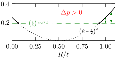
Figure 3: For contact angle $\theta_{-}$, Eq. (15) requires that $\left(\tilde{R}-1/2\right)^{2}\geq\frac{1}{4}\cos^{2}\theta_{-}$. Thus, the solid black curves cover possible values of $\tilde{R}$ for this $\theta_{-}$, and displacements upward from the green horizontal line, i.e., the arrows, show values of $\left(\tilde{r}_{-}-\sin\theta_{-}/2\right)^{2}$. The $\theta_{-}$ adopted for this drawing is $\pi/6$ as for the bottom branch shown in FIG. 2, and the right-most dot locates the value of the waist radius there (FIG. 2). Thus, the waist in that example is the slimmest waist in that range. Such considerations apply to both top and bottom contacts with their distinct contact angles. A contact angle near $\pi/2$ will correspond to a lower level for the horizontal line, and thus be less restrictive of the possible values of a common waist radius $\tilde{R}$.

II.2 More generally but $\Delta p\neq 0$

Restoring in Eqs. (14) and (15) the dependence on $\ell=2\gamma/\Delta p$ for $\Delta p\neq 0$, though possibly negative, then gives

$$r_{-}\left(r_{-}-\ell\sin\theta_{-}\right) = R\left(R-\ell\right),$$ (16a)

$$\left(R-\frac{\ell}{2}\right)^{2}=\left(r_{-}-\frac{\ell\sin\theta_{-}}{2}\right)^{2}\\ +\left(\frac{\ell\cos\theta_{-}}{2}\right)^{2}.$$ (16b)

$\ell$ is a signed length here. With these notations,

$$\cot^{2}\theta=\frac{r^{2}\ell^{2}-\left[r^{2}-r_{-}\left(r_{-}-\ell\sin\theta_{-}\right)\right]^{2}}{\left[r^{2}-r_{-}\left(r_{-}-\ell\sin\theta_{-}\right)\right]^{2}}\\ =\left(\frac{\mathrm{d}r}{\mathrm{d}z}\right)^{2}$$ (17)

and

$$\pm\mathrm{d}z=\frac{\left[r^{2}-r_{-}\left(r_{-}-\ell\sin\theta_{-}\right)\right]\mathrm{d}r}{\sqrt{r^{2}\ell^{2}-\left[r^{2}-r_{-}\left(r_{-}-\ell\sin\theta_{-}\right)\right]^{2}}}$$ (18)

separates these variables for integration.

We can still follow scaled lengths $\tilde{r}=r/\left|\ell\right|$ and $\tilde{R}=R/\left|\ell\right|$. Then the analogue of Eq. (15) is

$$\left(\tilde{R}+\frac{1}{2}\right)^{2}=\left(\tilde{r}_{-}+\frac{\sin\theta_{-}}{2}\right)^{2}+\left(\frac{\cos\theta_{-}}{2}\right)^{2}~{},$$ (19)

when $\Delta p<0$; see FIG. 4. The analogue of Eq. (18) with this length scaling for $\Delta p<0$ is

$$\pm\mathrm{d}\tilde{z}=\frac{\left[\tilde{r}^{2}-\tilde{r}_{-}\left(\tilde{r}_{-}+\sin\theta_{-}\right)\right]\mathrm{d}\tilde{r}}{\sqrt{\tilde{r}^{2}-\left[\tilde{r}^{2}-\tilde{r}_{-}\left(\tilde{r}_{-}+\sin\theta_{-}\right)\right]^{2}}}$$ (20)

To achieve $\Delta p/\gamma=1/R-\ddot{r}<0$ for a bridge with wiast radius $R$, clearly the curvature $\ddot{r}$ at that waist should be substantially positive to ensure that the negative second contribution dominates. In addition, the radius at the waist should be fairly large, thereby reducing the contribution of the positive first term. These points combined suggest that to achieve adhesion the contact areas should be larger than the waist area, which itself should be substantial.

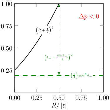
Figure 4: Analog of FIG. 3 but for the case $\Delta p<0$. See Eq. (19).

II.3 Waist $R$

Reaffirming the identification of $R$ as the radius of a waist, and specifically recalling that $\ell$ is a signed length:

$$\cot^{2}\theta\left(z\right)=\frac{r^{2}\ell^{2}-\left[\ell R+\left(r^{2}-R^{2}\right)\right]^{2}}{\left[\ell R+\left(r^{2}-R^{2}\right)\right]^{2}}=\left(\frac{\mathrm{d}r}{\mathrm{d}z}\right)^{2}~{}.$$ (21)

Factoring-out the $\cot^{2}\theta\left(\tilde{r}^{2}=\tilde{R}^{2}\right)=0$ feature gives

$$\cot^{2}\theta\left(z\right)=\frac{\left(R^{2}-r^{2}\right)\left(r^{2}-(R-\ell)^{2}\right)}{\left[r^{2}-R\left(R-\ell\right)\right]^{2}}=\left(\frac{\mathrm{d}r}{\mathrm{d}z}\right)^{2}~{}.$$ (22)

Eq. (22) also shows that $\cot^{2}\theta\left(z\right)=0$ at the point $r^{2}=(R-\ell)^{2}$.

Eq. (22) then achieves the separation of variables

$$\pm\mathrm{d}z=\frac{\left[r^{2}-R\left(R-\ell\right)\right]\mathrm{d}r}{\sqrt{\left(R^{2}-r^{2}\right)\left(r^{2}-\left(R-\ell\right)^{2}\right)}}$$ (23)

for integration in this case.

III Examples

In the example FIG. 2 ($\Delta p>0$), $\tilde{R}\approx 0.933$ and $\left(\tilde{R}-1\right)^{2}\approx 0.067{\,}^{2}$, smaller than the radius of the upper cross-section, $0.08{\,}^{2}$, in that extended example. The slimmer second waist is not realized.

FIG. 5 shows a bridge shape for the slender waist identified for the contact angles specified in FIG. 6 for $\Delta p>0$.

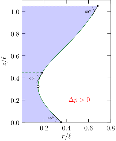
Figure 5: Capillary bridge shape for the biggest slim-waisted possibility of FIG. 6. Here the pressure inside is greater than the pressure outside. The open circle marks the waist. $\Delta p/\gamma=1/R-\ddot{r}$ at a waist of radius $R$, so achieving $\Delta p>0$ with positive curvature $\ddot{r}$, as above, limits the waist radius $R$. This solution exhibits the upper contact angle twice.

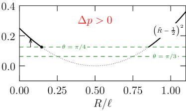
Figure 6: Considerations for choice of waist radii $\tilde{R}$ for the slim-waisted bridge of FIG. 5.

In the example FIG. 7, $\Delta p<0$ and $\ell<0$. Thus $\left(R-\ell\right)=|\ell|\left(\tilde{R}+1\right)$, and the $(-)$ of Eq. (23) is required to achieve a positive slope at the bottom plate. The aspect ratio of the bridge is vastly changed, as was true also in the discussion of capillary adhesion of Ref. 2; capillary adhesion would be expected for this shape.

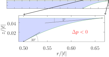
Figure 7: From Eq. (23), with the indicated contact angles and with $\Delta p<0$, so that pressure inside the bridge is less than the pressure outside. $\tilde{R}\approx 0.366$, from Eq. (19) and FIG. 4. Since the smallest contact radius — at the bottom plate — is 0.5, the waist at $\tilde{R}\approx 0.366$ is not realized in this physical range.

IV Discussion

In view of the variety of interesting shape possibilities, we reserve explicit study of the consequent inter-plate forces for a specific experimental context. Nevertheless, we outline here how such a practical study might be implemented.

The setup above permits straightforward calculation of the thermodynamic potential $\Omega$, and

$$\frac{\mathrm{d}\Omega}{\mathrm{d}h}=\left\langle\frac{\mathrm{d}U}{\mathrm{d}h}\right\rangle=-F_{h}~{}.$$ (24)

$U$ being the internal energy, positive values of $F_{h}$ indicates that $U$ decreases with increasing $h$, temperature being constant in these considerations. Thus, positive values of $F_{h}$ indicate repulsion, and negative values describe attraction.

Our motivating example is Cremaldi, et al.;¹ in those cases a waist with radius $\tilde{R}$ is clear, and we anticipate that $\Delta p>0$. To connect to specific experimental cases, we note that a priori experimental data are $\gamma$, the contact angles $\theta_{-}$ and $\theta_{+}$, the experimental volume of the captured droplet $v$, and inter-plate separation $h$. Eq. (15) and FIG. 3 show permitted ranges for $\tilde{R}$. With these parameters set, integration (Eq. (23)) determines $\Delta\tilde{z}=\tilde{z}_{+}-\tilde{z}_{-}$. Then

$$h=\left|\ell\right|\Delta\tilde{z}~{},$$ (25)

so that

$$\frac{1}{\left|\ell\right|}=\frac{\left|\Delta p\right|}{2\gamma}=\frac{\Delta\tilde{z}}{h}~{},$$ (26)

matching the experimental $h$. [What is more, the sign of $\Delta p$ is known through the calculational procedure.] We then further evaluate the volume of droplet

$$v\left[\tilde{R}\right]=\left|\ell\right|^{3}\pi\int\limits_{\tilde{z}_{-}}^{\tilde{z}_{+}}\tilde{r}^{2}\left(\tilde{z}\right)\mathrm{d}\tilde{z}~{}$$ (27)

as it depends on $\tilde{R}$, and seek a match with the experimental droplet volume $v$. If $\tilde{R}$ were provided a priori, Eqs. (26) and (27) would over-determine $\ell$. But $\tilde{R}$ is not provided a priori, so those two equations determine the two remaining parameters $\ell$ and $\tilde{R}$. Since the dependence on $\left|\ell\right|$ is clear, we can proceed further to

$$v\left[\tilde{R}\right]=\left(\frac{h}{\Delta\tilde{z}}\right)^{3}\pi\int\limits_{\tilde{z}_{-}}^{\tilde{z}_{+}}\tilde{r}^{2}\left(\tilde{z}\right)\mathrm{d}\tilde{z}~{},$$ (28)

leaving finally

$$\pi\int\limits_{\tilde{z}_{-}}^{\tilde{z}_{+}}\tilde{r}^{2}\left(\tilde{z}\right)\mathrm{d}\tilde{z}/\Delta\tilde{z}\;{}^{3}=\frac{v_{0}}{h^{3}}$$ (29)

to be solved for $\tilde{R}$.

V Conclusions

We provide general, simple, variable-separated quadrature formulae (Eq. (23)) for the shapes of capillary bridges, not necessarily symmetric. The technical complications of double-ended boundary conditions on the shapes of non-symmetric bridges are addressed by studying waists in the bridge shapes, noting that these relations change distinctively with change-of-sign of the inside-outside pressure difference of the bridge (Eq. (16b)). These results permit a variety of different interesting cases, and we discuss how these analyses should be implemented to study forces resulting from capillary bridging between neighboring surfaces in solutions.

References

- Cremaldi et al. (2015) Cremaldi, J. C., Khosla, T., Jin, K., Cutting, D., Wollman, K., and Pesika, N. (2015) Interaction of Oil Drops with Surfaces of Different Interfacial Energy and Topography. Langmuir 31, 3385 – 3390.
- deGennes et al. (2013) deGennes, P.-G., Brochard-Wyart, F., and Quéré, D. Capillarity and Wetting Phenomena: Drops, Bubbles, Pearls, Waves; Springer Science & Business Media, 2013.
- Lv and Shi (2018) Lv, C., and Shi, S. (2018) Wetting states of two-dimensional drops under gravity. Phys. Rev. E 98, 042802 – 10.
- Wallqvist et al. (2001) Wallqvist, A., Gallicchio, E., and Levy, R. M. (2001) A Model for Studying Drying at Hydrophobic Interfaces: Structural and Thermodynamic Properties. J. Phys. Chem. B 105, 6745–6753.
- Huang et al. (2003) Huang, X., Margulis, C. J., and Berne, B. J. (2003) Dewetting-induced collapse of hydrophobic particles. Proc. Natl. Acad. Sci. USA 100, 11953–11958.
- Huang et al. (2006) Huang, X., Margulis, C. J., and Berne, B. J. (2006) Correction for Huang et al., Dewetting-induced collapse of hydrophobic particles. Proc. Natl. Acad. Sci. USA 103, 19605–19605.
- Choudhury and Pettitt (2005) Choudhury, N., and Pettitt, B. M. (2005) On the Mechanism of Hydrophobic Association of Nanoscopic Solutes. J. Am. Chem. Soc. 127, 3556–3567.
- Cerdeiriña et al. (2011) Cerdeiriña, C. A., Debenedetti, P. G., Rossky, P. J., and Giovambattista, N. (2011) Evaporation Length Scales of Confined Water and Some Common Organic Liquids. J. Phys. Chem. Letts. 2, 1000 – 1003.
- Dzubiella et al. (2006) Dzubiella, J., Swanson, J., and McCammon, J. (2006) Coupling nonpolar and polar solvation free energies in implicit solvent models. J. Chem. Phys. 124, 084905.
- Bharti et al. (2016) Bharti, B., Rutkowski, D., Han, K., Kumar, A. U., Hall, C. K., and Velev, O. D. (2016) Capillary bridging as a tool for assembling discrete clusters of patchy particles. J. Am. Chem. Soc. 138, 14948–14953.
- Goldstein (1950) Goldstein, S. Classical Mechanics; Addison-Wesley, Reading, 1950; Chapt. 2.