Predicting CMEs using ELEvoHI with STEREO-HI beacon data
Abstract
Being able to accurately predict the arrival of coronal mass ejections (CMEs) at Earth has been a long-standing problem in space weather research and operations. In this study, we use the ELlipse Evolution model based on Heliospheric Images (ELEvoHI) to predict the arrival time and speed of 10 CME events that were observed by HI on the STEREO-A spacecraft between 2010 and 2020. Additionally, we introduce a Python tool for downloading and preparing STEREO-HI data, as well as tracking CMEs. In contrast to most previous studies, we use not only science data, which have a relatively high spatial and temporal resolution, but also lower-quality beacon data, which are — in contrast to science data — provided in real-time by the STEREO-A spacecraft. We do not use data from the STEREO-B spacecraft. We get a mean absolute error of 8.81 3.18 h / 59 31 km s-1 for arrival time/speed predictions using science data and 11.36 8.69 h / 106 61 km s-1 for beacon data. We find that using science data generally leads to more accurate predictions, but using beacon data with the ELEvoHI model is certainly a viable choice in the absence of higher resolution real-time data. We propose that these differences could be minimized if not eliminated altogether if higher quality real-time data were available, either by enhancing the quality of the already available data or coming from a new mission carrying a HI instrument on-board.
Space Weather
Space Research Institute, Austrian Academy of Sciences, Schmiedlstraße 6, 8042 Graz, Austria
Institute of Physics, University of Graz, Universitätsplatz 5, 8010 Graz, Austria
RAL Space, STFC Rutherford Appleton Laboratory, Didcot, UK
Maike Bauermaike.bauer@oeaw.ac.at
The viability of using the ELEvoHI model with lower-quality real-time data was studied
We find that using real-time data with ELEvoHI is possible, but CME prediction benefits significantly from improved data quality
We find that using real-time data with ELEvoHI is possible, but coronal mass ejection prediction benefits significantly from improved data quality
Plain Language Summary
Coronal mass ejections (CMEs) are large ejections of plasma and the accompanying magnetic field caused by magnetic activity on the Sun. If CMEs reach Earth, they interact with the planetary magnetic field. In doing so, CMEs can cause disturbances to power grids and other electrical infrastructure on our planet, inhibit radio transmissions and damage satellites, which is why it is important to have an accurate way of predicting the arrival of the phenomena. Our model uses data provided by the HI cameras on the STEREO spacecraft. These data are available in a lower quality in real-time, i.e. within a latency of about 5 minutes within being received at the ground station, or in a higher quality with a delay of around 3 days. Using real-time data is important if we want to be able to predict the arrival of CMEs in a timely manner. In this study, we show that we can use the lower-quality real-time STEREO-HI data to make accurate predictions of the arrival time of CMEs.
1 Introduction
Coronal mass ejections (CMEs) are explosive outbursts of plasma and the accompanying magnetic field from the Sun. The expelled material moves at high speeds throughout the heliosphere and interacts with any obstacles, such as planets and their magnetospheres, along the way. If a CME reaches Earth, various phenomena, summarized under the term space weather, can be observed. These phenomena can range from harmless to destructive in their intensity. CMEs may induce strong geomagnetic storms that have a significant impact on satellites in orbit and electrical devices on the planet’s surface as well as the ability to cause disturbances in radio transmissions. As our world becomes more and more reliant on technology and thus a continuous supply of electricity to power it, the importance of real-time ICME predictions is increasing (Cannon, \APACyear2013; Oughton \BOthers., \APACyear2017).
A variety of modelling techniques have been developed for this purpose. In the following, we give a short overview focusing on models that rely on heliospheric imagers on board the STEREO spacecraft. Examples include Fixed-Phi Fitting (FPF; Rouillard \BOthers., \APACyear2008; Sheeley \BOthers., \APACyear1999), which assumes that the CME is a point moving radially away from the Sun at constant speed in a fixed direction and Harmonic Mean Fitting (HMF; Lugaz \BOthers., \APACyear2009; Lugaz, \APACyear2010), which makes the same assumptions as FPF but treats the CME as an expanding sphere with the center tethered to the Sun. For Self-Similar Expansion Fitting (SSEF; Davies \BOthers., \APACyear2012; Möstl \BBA Davies, \APACyear2013), the width of the CME may be freely chosen anywhere between 0∘, in which case it is identical with FPF, and 180∘, in which case it is equivalent to HMF.
While FPF, HMF and SSEF methods can provide an estimate of the CME’s propagation direction and speed based on single-spacecraft HI observations, multi-point views can be exploited to reduce the assumptions necessary. The “triangulation” class of methods assumes the same geometries used in FPF (Liu \BOthers., \APACyear2010), HMF (Lugaz, \APACyear2010) and SSEF (Lugaz, \APACyear2010; Davies \BOthers., \APACyear2013). As was recently shown by Hinterreiter \BOthers. (\APACyear2021), the assumption of a fixed shape for CMEs can lead to differences in arrival time predictions depending on which spacecraft is used as imaging input within the model.
Slightly more sophisticated models may employ drag-based fitting. Such methods assume that the kinematics of a CME (which are dominated by the Lorentz force close to the Sun) are governed by the ambient solar wind flow as the transient moves away from the Sun. CMEs that are faster than the ambient solar wind are slowed down while slower ones speed up (Cargill, \APACyear2004; Vršnak \BOthers., \APACyear2013). A model building on this assumption is the Drag-based Ensemble Model (DBEM) first introduced by Dumbović \BOthers. (\APACyear2018). It produces a range of outcomes for the arrival time and speed of the CME. The Ellipse Evolution Model based on Heliospheric Imager data (ELEvoHI; Rollett \BOthers., \APACyear2016; Amerstorfer \BOthers., \APACyear2018, \APACyear2021) which is used in this paper is based on observations made using the Heliospheric Imagers (HI; Eyles \BOthers., \APACyear2009) aboard the STEREO spacecraft. ELEvoHI incorporates drag-based model fitting and is able to give estimates for certain input parameters due to its use of HI observations. This method will be described in greater detail in Section 3.
Models for the prediction of CME parameters may also be empirical in nature, using parameters observed in situ to make predictions. One such model is the Effective Acceleration Model (EAM; Paouris \BBA Mavromichalaki, \APACyear2017), which relies on the SOHO/LASCO and ACE spacecraft. More computationally intense models rely upon the solution of the magneto-hydrodynamic (MHD) equations. These include, for example, ENLIL (Odstrčil \BOthers., \APACyear2004) and EUHFORIA (Pomoell \BBA Poedts, \APACyear2018), which can be coupled with different coronal models, such as (WSA; Arge \BOthers., \APACyear2003), Magnetohydrodynamics Algorithm outside a Sphere (MAS; Linker \BOthers., \APACyear1999) and MULTI-VP (Pinto \BBA Rouillard, \APACyear2017).
Models predicting the arrival time of CMEs are being improved continuously. To be of use for establishing a system that could give an advance warning of the arrival of an Earth directed CME, models must be able to predict such events in real-time. The prediction models that are currently operational mostly make use of coronagraph data from the Large Angle and Spectrometric Coronagraph (LASCO) aboard the Solar and Heliospheric Observatory (SOHO), which sits at L1 and has a field of view (FOV) of about 30 R⊙ in all directions. Data from the COR2 coronagraph aboard STEREO-A are also used frequently. There are already models predicting the arrival of CMEs in real time that have been operating for years, e.g. WSA-ENLIL+Cone (Odstrčil \BOthers., \APACyear2004). Wold \BOthers. (\APACyear2018) assessed the performance of the WSA-ENLIL+Cone model for 273 CMEs that occurred between March 2010 and December 2016 and found a mean absolute arrival time error of 10.4 ± 0.9 hours. Möstl \BOthers. (\APACyear2017) analyzed 1337 CME events from a period of 8 years and predicted their arrival time using the SSE technique. This approach yielded an absolute arrival time error of 2.6 ± 16 h and found that prediction accuracy for STEREO-HI science data slightly increases with increasing longitudinal observer angle. There is, however, no current model that allows for real-time predictions using the STEREO-HI instruments.
The STEREO-HI instruments benefit from a larger FOV compared to coronagraphs, which are centered on the Sun directly and mostly observe the solar corona. Additionally, STEREO-HI has the ability to view Earth-directed CMEs side-on when at or near the L4 or L5 orbital points, instead of only head-on as a coronagraph would, resulting in a better view of their structure. These benefits could improve the accuracy of CME arrival predictions and decrease the number of false alarms. CME kinematics may change considerably due to interactions with the solar wind and/or other CMEs during their interplanetary propagation, making prolonged observation of the event advantageous (Colaninno \BOthers., \APACyear2013). Unfortunately, real-time data from the STEREO-HI instruments are only available in low-rate beacon data (Biesecker \BOthers., \APACyear2008). These lower-quality data make real-time observation of a CME further away from the Sun more difficult.
Tucker-Hood \BOthers. (\APACyear2015) have previously used beacon data in combination with FPF as part of the Solar Storm Watch (SSW) citizen science project to analyze the effect that the use of real-time data have on predictions of arrival speed and transit time. For the 20 CMEs that arrived at Earth, they obtained an arrival speed error of 151 km s-1 and a transit time error of 22 h. By taking interplanetary acceleration of the CME into account, they were able to reduce the error to 77 km s-1 for the arrival speed and 19 h for the transit time. These errors were attributed to a mix of technical issues with the real-time data, such as the low spatial and temporal resolution, and physical issues with the propagation of CMEs. Furthermore, Davis \BOthers. (\APACyear2011) obtained an arrival time error of + 12.98 h for the 8 April 2010 event, which is also studied in this paper, using STEREO-B HI beacon data.
Using ELEvoHI, we expect to see results similar to those in previously mentioned studies in terms of arrival time and speed errors for predictions based on science data. Outcomes for predictions based on beacon data are expected to be worse than those based on science data. The general aim of space weather predictions is giving accurate arrival time and speed estimates for CMEs in real-time, so as to ensure a reliable way of alerting interested parties to an oncoming CME before it actually arrives. ELEvoHI is constantly being improved in terms of accuracy, most recently trough the incorporation of frontal deformation for CMEs by Hinterreiter \BOthers. (\APACyear\bibnodate). The implementation of predictions using beacon data for ELEvoHI would add to the tool’s repertoire and be a step towards true real-time predictions of CME arrival time and speed.
In Section 2, we give an overview of the data we use and how they were prepared. In Section 3, we describe the basic components of the ELEvoHI model. In Section 4 we present our results and describe the differences between predictions made using STEREO-HI science images and the so-called beacon data (real-time data) in detail. The results are discussed in Section 5. Section 6 provides a summary and a conclusion of our work.
2 Data
2.1 The STEREO mission
The twin-spacecraft STEREO-A(head) and STEREO-B(ehind) were launched in 2006 to improve our understanding of various space weather phenomena, including CMEs and particularly those CMEs that are Earth directed (Kaiser \BOthers., \APACyear2008). STEREO-A moves on an orbit inside the Earth’s orbit around the Sun, while STEREO-B’s orbit lies slightly further out. The difference in orbital distance is small, i.e. both spacecrafts’ orbit close to 1 AU from the Sun, but large enough for STEREO-B to lag behind STEREO-A in its orbit around the Sun. This leads to the two spacecraft attaining an increasing angular separation, which allows for observing space weather phenomena from two distinct vantage points. The focus of this paper lies on the use of STEREO-A data. Contact with STEREO-B was lost in 2014 after a test of the spacecraft’s command loss timer before it entered into a period of solar conjunction.
In this work, we make use of STEREO’s Sun Earth Connection Coronal and Heliospheric Investigation (SECCHI; Howard \BOthers., \APACyear2008) suite of instruments, which consists of two white-light imagers with overlapping FOV, called heliospheric imagers (HI1 and HI2; Eyles \BOthers., \APACyear2009) as well as two white-light coronagraphs, COR1 and COR2 (Thompson \BOthers., \APACyear2003; Howard \BOthers., \APACyear2008), and one EUV-camera (EUVI; Wuelser \BOthers., \APACyear2004). The FOV of the two HI instruments is measured in degrees of elongation. Elongation gives the angle between the observer, Sun-centre and another object. 0∘ of elongation corresponds to an object directly on the observer-Sun line. HI1 has a FOV extending from roughly 4∘ to 24∘ elongation when measured from the Sun center, giving it a FOV of 20 x 20 ∘. HI2 has a FOV extending from 18.8∘ to 88.8∘ elongation, amounting to a FOV of 70 x 70 ∘. These values are valid in the ecliptic plane during nominal operations. The time cadence differs between data types and instruments, with HI1 science data having a cadence of 40 minutes and HI1/HI2 beacon data as well as HI2 science data having a cadence of 120 minutes.
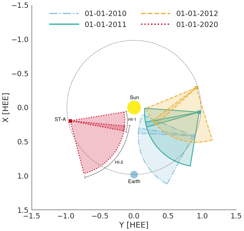
To test the viability of making real-time predictions using STEREO-HI beacon data with the ELEvoHI model, we analyze 10 CMEs observed by the STEREO-A spacecraft between 2010 and 2020. We chose the events because they have been extensively studied before (except for the 9 July 2020 event) and are particularly well visible in STEREO-HI science data (Möstl \BOthers., \APACyear2014; Rollett \BOthers., \APACyear2016). Furthermore, they encompass a variety of dates with data captured from different positions of STEREO-A’s orbit. The orbital position of STEREO-A for each year in which one of the selected events occurs is depicted in Figure 1.
Data transmitted by STEREO’s space weather beacon are of considerably lower quality than regular science data. Science data are transferred at regular intervals upon contact with the Deep Space Network (DSN) while beacon data are continually broadcast to a number of cooperating antenna stations around the world. Due to the limitations in telemetry allocated to the real-time beacon mode, HI2 beacon data undergo Rice lossless compression while HI1 data are compressed using ICER lossy compression. Furthermore, convolutional 1/6 encoding (changed from convolutional 1/2 encoding on 27 July 2007) is used to ensure reliable data transfer for beacon data and reduce errors in transmission. Both forms of data are uploaded in near-real time onto the internet after being downlinked and are subsequently processed into Flexible Image Transport System (FITS) files at the STEREO Science Center. The images are made available to the public as soon as this process is finished, which means that beacon data are available in near real-time (Eichstedt \BOthers., \APACyear2008).
2.2 Data preparation
The images used in this work go through extensive pre-processing to minimize any residual noise and make the CMEs as clearly visible as possible. Usually, data correction and calibration of STEREO/HI images is done in part by using the routine, written in IDLTM SolarSoft. The data reduction procedures contained therein were adapted for the Python programming language for this paper and are available online as open-source code (see Section 7). Using a freely available open-source programming language ensures that reproducibility of results is not contingent on access to software via an institutional subscription. A brief overview of the most important steps is given below.
Both science and beacon images are already processed aboard the STEREO spacecraft, but this will not be discussed further at this point. For a detailed description of the on-board processing, please refer to Eyles \BOthers. (\APACyear2009). Science and beacon data are treated largely equally during the on-ground data reduction process. In the beginning, saturated columns are masked. Saturation often occurs when planets are in the imagers FOVs. Neither HI1 nor HI2 utilize camera shutters, so smearing effects that will occur due to this circumstance must be corrected. To be able to easily interpret the image data, a calibration factor can be applied that converts the units of the pixels from DN/sec to units of mean solar brightness. A flatfield is subtracted from the images and distortion correction is done to account for the HI cameras wide-angle optics. As one of the last steps, the spacecraft’s pointing information is updated by fitting the image to known stars.
In order to obtain the time-elongation profile necessary for making predictions with the ELEvoHI model, time-elongation-plots are created from the L1 processed images obtained from the Python program. Tracking can also be done directly in L1 HI images. This is sometimes the case for studies investigating individual CME events, as for example in Rollett \BOthers. (\APACyear2014). Producing a time-elongation map (J-Map; Davies \BOthers., \APACyear2009; Sheeley \BOthers., \APACyear1999) is accomplished by extracting a strip from the image with a fixed width of 5∘ in position angle centered on the ecliptic plane. This process is completed for each of the images in the time-series. The strips obtained this way are stacked next to each other, producing a J-Map. We use running difference images to further enhance the visibility of the CMEs under study. This produces the final J-Map in which the leading edge of the CME is clearly visible as a bright streak.
3 Methods
ELEvoHI was first introduced by Rollett \BOthers. (\APACyear2016) as a combination of the ELlipse Evolution model (ELEvo; Möstl \BOthers., \APACyear2015) and drag-based model fitting (DBM fitting) that can be used to predict arrival time and speed of CMEs at various points within the heliosphere. The authors showed that the addition of the solar wind drag leads to improvements in CME prediction, particularly in terms of arrival speed, when compared to previously described methods such as FPF, HMF or SSEF (Rollett \BOthers., \APACyear2016). ELEvoHI was first presented as a single-run model, but has since been updated to employ an ensemble approach (Amerstorfer \BOthers., \APACyear2018, \APACyear2021).
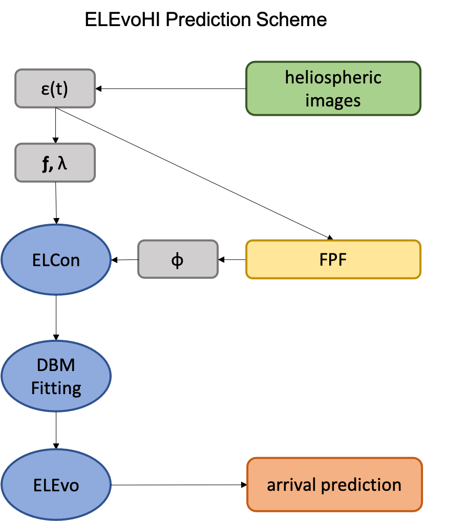
ELEvoHI consists of three main methods, ELlipse Conversion (ELCon), DBM fitting and ELEvo. DBM fitting and ELCon provide parameters for ELEvo in order to generate predictions for CME arrival time and speed. Figure 2 presents an overview of how the modules within ELEvoHI relate to each other. A time-elongation track of the CME is required as input. Such a track is obtained by tracing the CME in J-Maps. To minimize the influence of human tracking deviations between tracks, we attempt to track each CME 5 times for each data type and event. These 5 tracks are then interpolated onto a common time grid via polynomial interpolation and averaged. The elongation profile must be converted to units of radial distance. In the ELEvoHI model, this task is taken on by ELCon which works under the assumption of an elliptical geometry for the CME. Similarly to SSE, the CMEs angular half-width, , can be freely chosen. Additionally, the inverse ellipse aspect ratio, , can be modified to change the curvature of the CME front. At = 1, the frontal shape is equal to that of a circle. As decreases, the front becomes flatter. The CME’s direction of motion, , must also be provided for ELCon to be able to accurately convert the elongation profile into a radial distance profile. ELCon is consistent with the assumption of an elliptical CME geometry and, in combination with ensemble modeling, allows for a variety of CME shapes to be considered for predictions.
In this study, a range of values for , and are used. and are estimated quantities in this study. Recently, Hinterreiter \BOthers. (\APACyear2021) introduced the Ecliptic cut Angles from Graduated Cylindrical Shell (Thernisien \BOthers., \APACyear2006) for ELEvoHI tool (EAGEL) which opens up the possibility of a better estimation of . We vary between 0.7 and 1.0 with a step size of 0.1. We vary over a range of 10∘ from the values acquired via the FPF method with a step size of 2∘. We vary between 30 and 50, with a step size of 5. After the conversion via ELCon, the aforementioned parameters serve as input for DBM fitting, a fitting technique based on the equations of the DBM. Additionally, DBM fitting requires the selection of a range of R(t) to consider. These ranges are manually selected for each event. This method delivers the ambient solar wind speed , the drag parameter , the initial radial distance and speed at time . is determined by inputting a range of background solar wind speeds (250 – 700 km s-1, in 25 km s-1 steps) and subsequently choosing the speed that yields the best DBM fit. These initial values are thus derived solely from the CME kinematics. The values are passed onto ELEvo, in combination with the angular half width and the inverse aspect ratio, which then predicts the arrival time and speed of the CME based on the assumption of an elliptical CME front with constant half-width and aspect ratio.
The selected CMEs are compared regarding the difference in predicted and in situ arrival time and speed. In situ arrival times for all events, except 9 July 2020, are taken from Möstl \BOthers. (\APACyear2014), which uses data from the Wind spacecraft (see Section 7) to determine arrival of a CME at L1 by using the shock arrival time as the CME arrival time. The in situ arrival time for the 9 July 2020 event was determined through similar means. The CME speed at L1 is also obtained from Wind data. It is taken to be the mean proton bulk speed of either of the aforementioned phenomena (that is the CME itself, or the shock ahead of the magnetic flux rope, MFR, or indeed the MFR itself).
4 Results
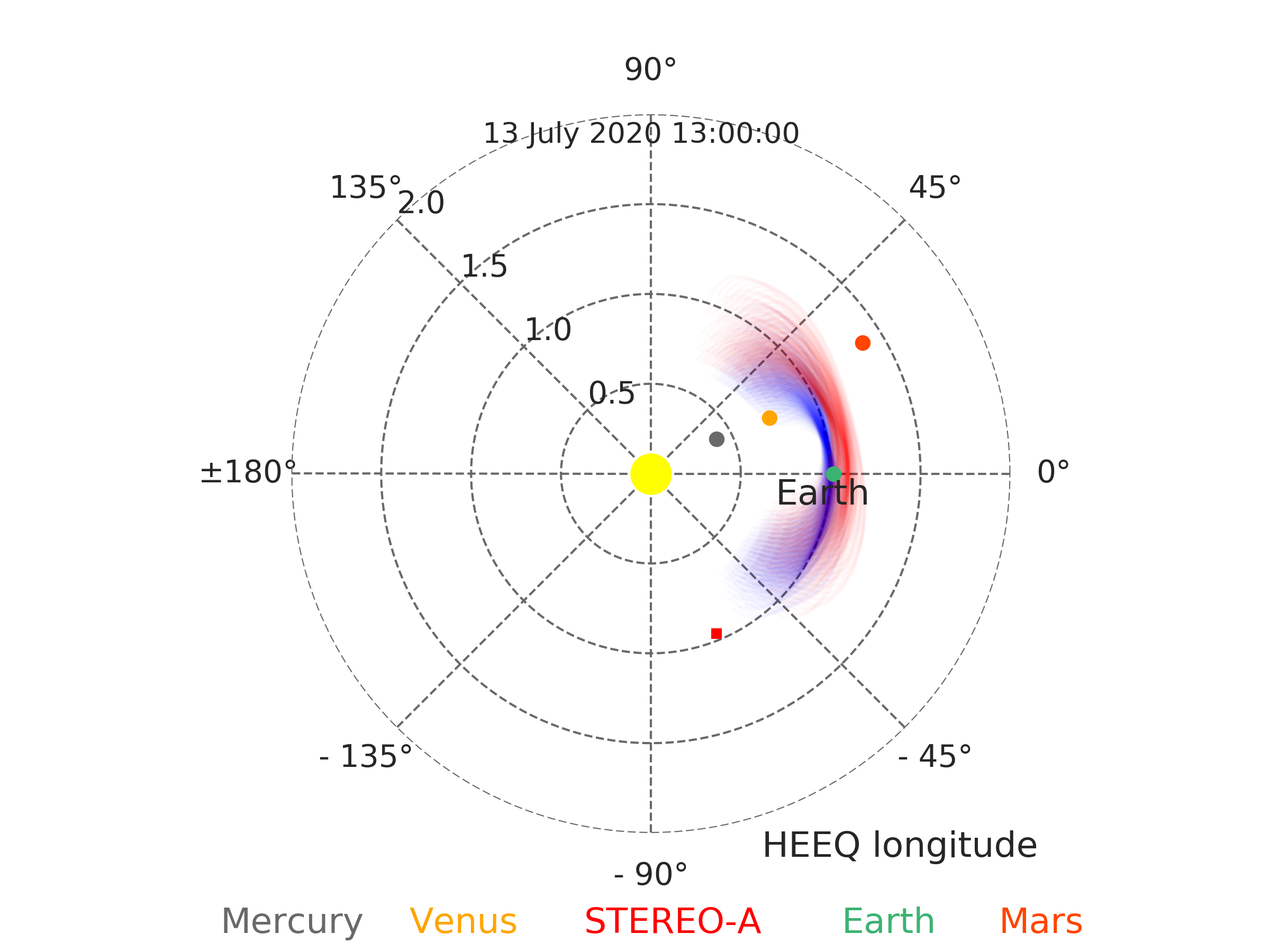
We perform ELEvoHI ensemble modeling for 10 CME events observed between the years of 2010 and 2020 by the STEREO-A spacecraft and compare the predicted arrival times and speeds obtained using science and beacon data to in-situ arrivals. Each ensemble run consists of 275 individual ensemble members. All selected CMEs propagated in or close to the ecliptic plane, making them clearly visible from STEREO-A’s perspective at the time of observation. The dates given for each event correspond to the date that the respective CME was first observed on in the STEREO-HI1 camera. Figure 3 shows a still image taken from a movie depicting the results of an ELEvoHI ensemble run for one of our selected events. Science data are marked in blue, while beacon data are shown in red. Each ensemble member is shown as an elliptical front moving outwards from the Sun. As this figure shows, there is variation within ensembles even for the same data type due to the use of differing CME parameters. It also shows the discrepancy between predictions based on science and beacon data, with ensemble members of this beacon data prediction generally arriving earlier than those of science data predictions.
4.1 Arrival time and speed predictions
As already described in the previous section, the time-elongation tracks are obtained by manually tracking the path of the CME front along the ecliptic in J-Maps resulting from the data reduction procedures. We do this 5 times for every event and data type (science and beacon); so there are a total of 10 tracks for each event. The 5 tracks of each data type are interpolated to lie along a regularly spaced time-axis and subsequently averaged to decrease the influence of human tracking errors on the result (more on this in Section 4.2). Figure 4 shows a comparison of J-Maps for science and beacon data. The J-Map produced using science data is clearly of superior quality, with much fewer data gaps and fainter structures also clearly visible.
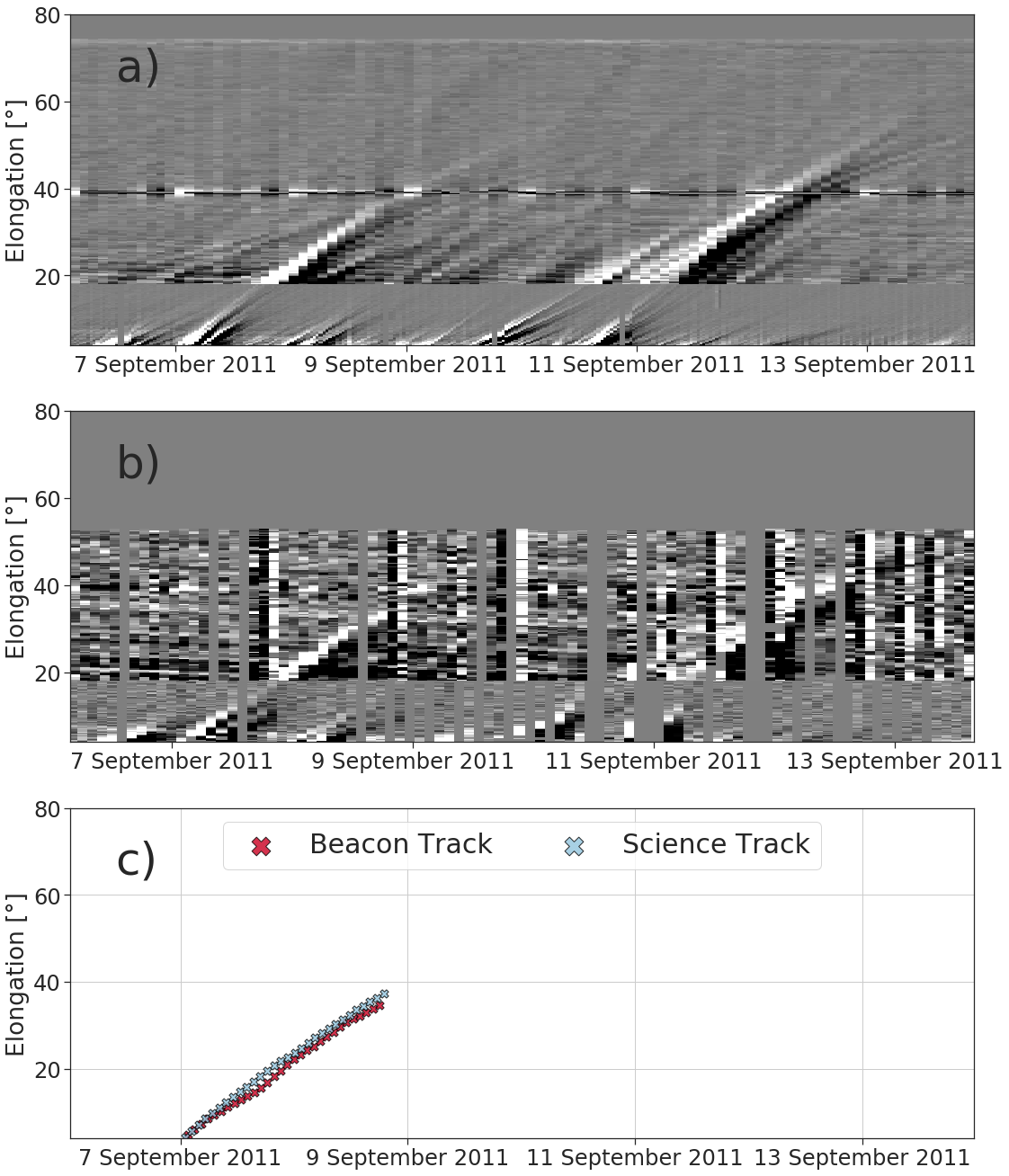
Figure 5 shows the distributions of the difference in predicted and in situ arrival time for all ten events as violin plots based on science (blue) and beacon (red) data. The error in hours for science data is given on the left-hand side of each violin in blue, while the error for beacon data for the same CME is given on the right-hand side in red. The dark horizontal line in each distribution marks the median value. Positive values indicate that the prediction made using ELEvoHI succeeds the actual in situ arrival, while negative values signify a premature prediction. The mean absolute error, MAE(t), of the arrival time predictions over all 10 CMEs made using science data is 8.8 h, the mean error, ME(t), is 6.2 h and the root mean square error, RMSE(t), is 8.9 h. The standard deviation, STD(t), of MAE(t) for science data is 3.2 h. The MAE(t) for beacon data is 11.4 h, the ME(t) is 7.3 h and the RMSE(t) is 13.9 h. The STD(t) of MAE(t) for beacon data is 8.7 h.
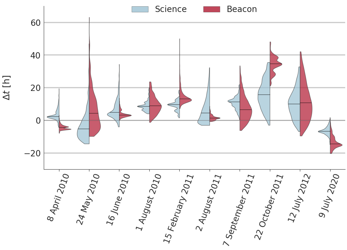
Looking at the ME(t) for each event suggests that ELEvoHI tends to predict a late arrival for science as well as for beacon data, when compared to the actual in situ arrival time. There are 4 exceptions to this observation: The ME(t) of the time-difference distribution obtained using beacon data of the 8 April 2010 CME, using science data of the 24 May 2010 CME and for both data types of the 9 July 2020 CME. All of these predictions are early, on average. The event which shows the largest discrepancy for both science and beacon data is 22 October 2011, with a deviation of 15.7 h for science and 34.7 h for beacon data, respectively. For science data, this is also the event possessing the largest standard deviation with a value of 8.9 h. For beacon data, the event with the largest standard deviation is 12 July 2012, with a value of 10.3 h. The ME(t)s, MAE(t)s and RMSE(t)s for , including each event’s standard deviations can be found in Table 1.
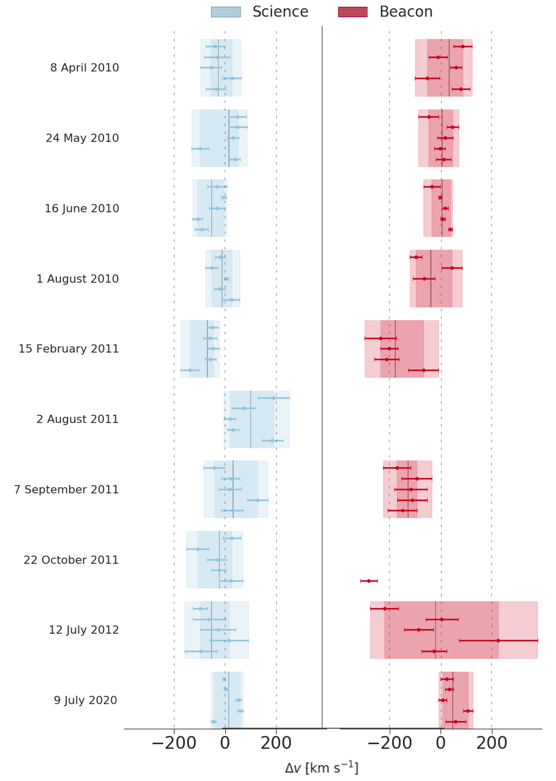
Figure 6 shows the distributions of the difference in predicted and in situ arrival speed at L1 for all ten events as violin plots based on science (blue) and beacon (red) data. The mean error in km s-1 for science data is given on the left-hand side of the violins in blue, beacon data is given on the right-hand side in red. The dark horizontal line in each distribution indicates the median value. Positive values signify that the speed predicted by ELEvoHI is higher than the actual in situ speed, while negative values indicate that the predicted speed was lower than that of the actual CME. The mean absolute error, MAE(v), of the arrival speed predictions made using science data is 59 km s-1, the mean error, ME(v), is -14 km s-1 and the root mean square error, RMSE(v), is 39 km s-1. The standard deviation of MAE(v), STD(v), is 31 km s-1. The MAE(v) for beacon data is 106 km s-1, the ME(v) is 17 km s-1 and the RMSE(v) is 111 km s-1. The STD(v) of MAE(v) is 61 km s-1.
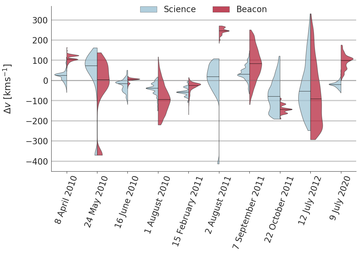
A particular bias in the predictions is less clear for speed predictions than it is for arrival time predictions. The ME(v)s indicate that ELEvoHI tends to predict an arrival speed that is slower than observed for science data and faster than observed for beacon data. It must be noted, however, that the numbers for the beacon data arrival speed are significantly influenced by the 2 August 2011 event which has an arrival speed error distribution that skews heavily towards a speed prediction that is too fast. The 2 August 2011 event has an MAE(v) of 246 km s-1, making it the event with the largest MAE(v) in terms of arrival speed of any event using beacon data. The largest MAE(v) for arrival speed for science data belongs to the 12 July 2012 event with 104 km s-1. The event which shows the largest standard deviation is 24 May 2010, for both science and beacon data, with a deviation of 91 km s-1 and 115 km s-1, respectively. The MAE(v)s including their standard deviations for all events can be found in Table 1.
Events ME(t) [h] MAE(t) [h] RMSE(t) [h] STD(t) [h] Science Beacon Science Beacon Science Beacon Science Beacon 8 April 2010 3.3 -4.2 3.7 4.3 4.8 4.5 3.1 1.4 24 May 2010 -3.0 6.6 7.7 10.0 9.6 14.0 5.8 9.8 16 June 2010 6.7 3.9 7.0 3.9 9.1 4.5 5.8 2.2 1 August 2010 8.9 9.5 8.9 9.5 9.4 11.0 3.2 5.5 15 February 2011 9.3 14.9 9.3 14.9 9.9 15.8 3.2 5.3 2 August 2011 6.1 1.7 7.0 1.8 9.9 2.4 6.9 1.6 7 September 2011 10.8 7.6 10.8 8.5 11.5 11.0 3.9 7.0 22 October 2011 15.9 34.3 16.0 34.3 18.3 34.6 8.9 5.1 12 July 2012 10.5 11.8 11.2 13.1 13.7 16.6 8.0 10.3 9 July 2020 -6.5 -13.3 6.5 13.3 6.9 13.8 2.5 3.9 Events ME(v) [km s-1] MAE(v) [km s-1] RMSE(v) [km s-1] STD(v) [km s-1] Science Beacon Science Beacon Science Beacon Science Beacon 8 April 2010 22 110 27 110 34 112 21 17 24 May 2010 36 -32 105 98 139 152 91 115 16 June 2010 -24 2 30 10 39 12 25 6 1 August 2010 -41 -89 42 98 52 113 31 57 15 February 2011 -56 -33 56 33 60 42 22 26 2 August 2011 5 245 60 245 96 246 75 17 7 September 2011 38 84 44 96 53 115 29 64 22 October 2011 -73 -142 89 142 105 144 55 21 12 July 2012 -32 -65 111 141 132 164 71 84 9 July 2020 -19 92 22 92 26 100 13 37
4.2 Influence of human tracking error
It is important to keep in mind that the time-elongation profiles describing the CME’s trajectory outward are obtained by tracing the perceived front of the CME by hand. The process is thus subject to human error. Different people may come up with disparate tracks in the end, even if guidelines are provided. Barnard \BOthers. (\APACyear2015) analyzed and compared three different methods for tracking CMEs (CMEs were tracked by experts, an algorithm or participants in the SSW citizen science program) and found that the method used introduced more variability into the assumed CME kinematics than the differences between several single-spacecraft fitting techniques did. Even if only one person is tasked with tracking the front, as was the case in this study, there is no guarantee that tracks will always be identical, although the difference between tracks generated by the same individual may be smaller than that of tracks coming from several people.
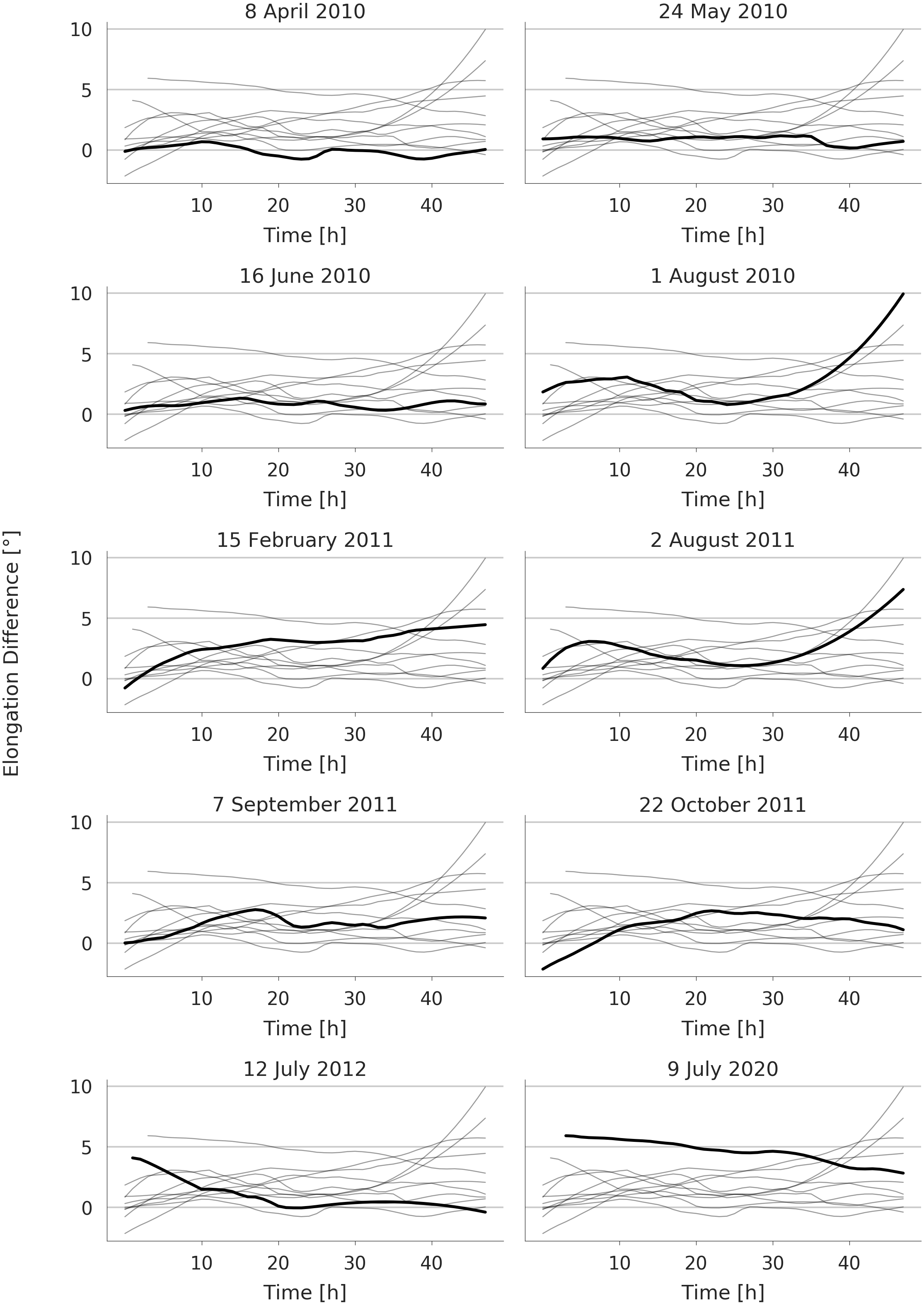
Figure 7 shows the difference between the averaged science and beacon time-elongation profiles for each event. The difference between the science and beacon tracks for each event at each point in time was calculated and is plotted against the time-axis. The thick line marks the difference in elongation for each event, while the fainter gray lines in the background represent the difference in elongation for all other dates which serve as a comparison. The event with the largest average difference between science and beacon data track is 9 July 2020. In contrast, the two tracks are almost identical for the 8 April 2010 event. On average, science data tracks have a larger elongation at the same point in time than their beacon data counterparts. There are 4 events (8 April 2010, 15 February 2011, 22 October 2011 and 12 July 2012) where tracks obtained from beacon data show a larger elongation for at least one point in time than tracks obtained using science data.
To investigate the influence that the deviations between individual tracks have on the overall outcome of the time and speed predictions, we input all 5 tracks for each data type and event separately into ELEvoHI and see how the results differ from each other. To be able to ascertain the differences between tracks for the same event, we look at the difference between predicted and in situ measurements of arrival time, , and arrival speed, . For the beacon data tracks of event 2 August 2011, no predictions from individual tracks based on science or beacon mode were possible, suggesting that this event benefited greatly from the interpolation and averaging of the 5 separate tracks. Furthermore, this event already displayed quite a large error in its beacon data arrival speed prediction over the ensemble members. Sometimes, tracks may simply not have enough data points or be too irregularly spaced, preventing ElEvoHI from making a prediction based on that track. Badly chosen starting points for the DBM fit or a poorly tracked time-elongation profile may also cause failed ELEvoHI predictions.
Figure 8 shows the distribution of for all ten CMEs in terms of their mean and standard deviation. in hours for science data is always given on the left-hand side in blue while it is given on the right-hand side marked in red for beacon data. The average MAE(t) of the predictions made using science data is 11.8 h. The average MAE(t) for predictions made using beacon data is 23.5 h. Science data have, on average, a considerably lower MAE(t) than beacon data. The largest MAE(t) for any event tracked in science data is 37.7 h obtained for event 24 May 2010; for beacon data it is event 22 October 2011 with a MAE(t) of 108.9 h.
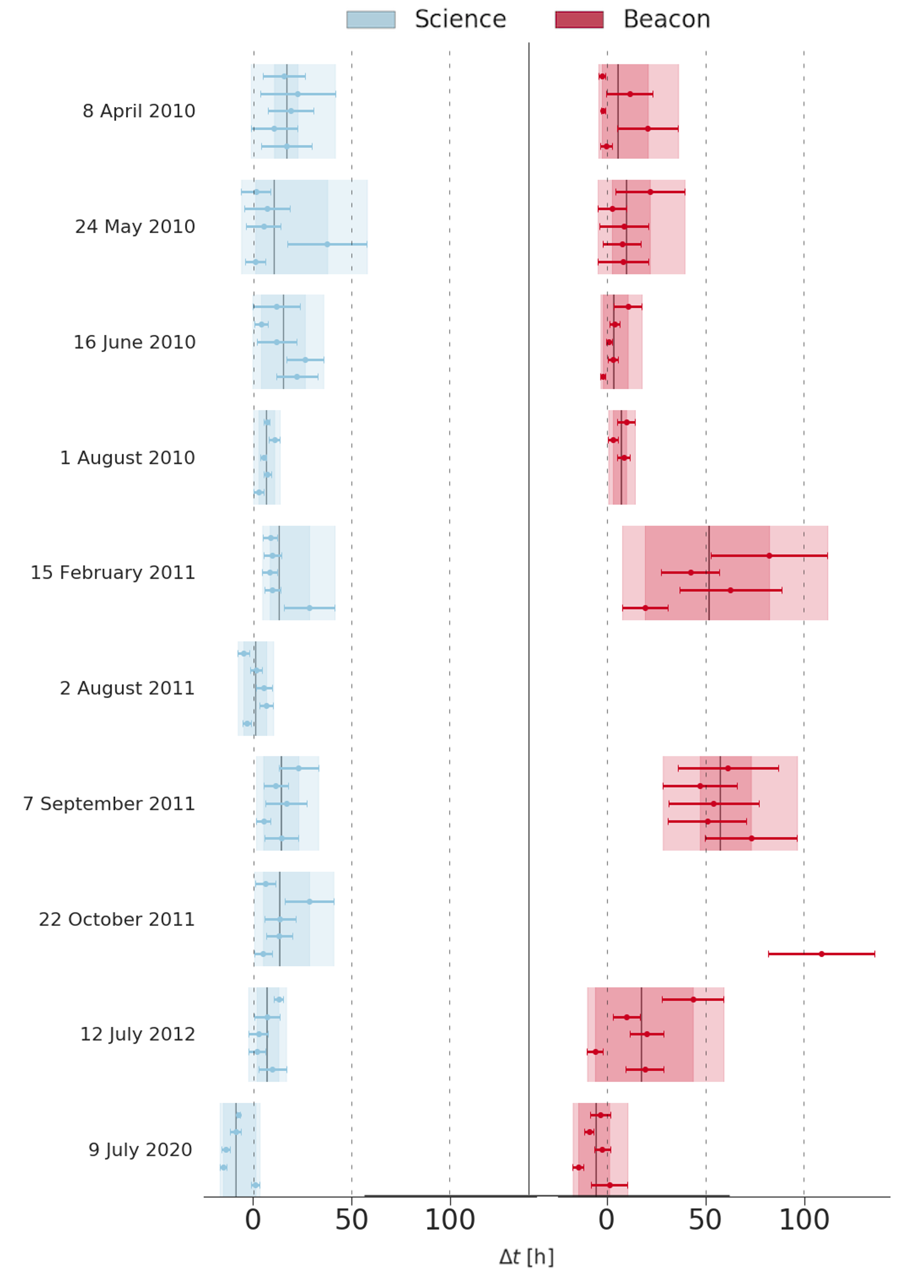
Figure 9 shows the same quantities as Figure 8 for . The average MAE(v) of the predictions made using science data is 66 km s-1. The average MAE(v) for predictions made using beacon data is 93 km s-1. The largest MAE(v) for any individual event tracked in science data is 189 km s-1 obtained for the 2 August 2011 event; for beacon data it is event 22 October 2011 with a MAE(v) of 281 km s-1. All results pertaining to the and can be found in Table 2 for science data and beacon data.
Events Track MAE(t) [h] STD(t) [h] MAE(v) [km s-1] STD(v) [km s-1] Science Beacon Science Beacon Science Beacon Science Beacon 8 April 2010 1 16.9 3.8 12.7 3.0 44 82 40 35 8 April 2010 2 11.3 20.8 11.8 15.4 64 58 37 47 8 April 2010 3 19.1 2.2 11.5 1.1 57 60 40 21 8 April 2010 4 22.7 11.8 19.0 11.8 68 44 50 36 8 April 2010 5 15.6 3.3 10.8 1.8 43 86 36 36 24 May 2010 1 5.1 10.3 5.2 12.8 42 48 20 30 24 May 2010 2 37.7 8.5 20.1 9.6 98 27 34 21 24 May 2010 3 8.2 10.9 8.8 12.5 43 51 24 29 24 May 2010 4 10.8 6.3 11.6 7.2 64 53 36 24 24 May 2010 5 7.9 21.9 7.4 17.6 57 54 34 40 16 June 2010 1 22.2 2.1 10.4 1.2 91 38 26 8 16 June 2010 2 26.3 3.4 9.4 2.7 108 13 19 9 16 June 2010 3 12.0 2.3 10.1 1.5 38 19 32 12 16 June 2010 4 4.1 3.9 3.4 2.5 14 12 10 6 16 June 2010 5 11.8 10.6 12.0 7.1 41 39 39 32 1 August 2010 1 3.1 - 2.7 - 53 - 32 - 1 August 2010 2 7.3 - 2.0 - 25 - 20 - 1 August 2010 3 5.2 8.6 1.4 3.2 16 71 8 43 1 August 2010 4 10.8 3.1 2.8 2.4 53 65 24 39 1 August 2010 5 7.0 9.8 1.6 4.4 22 97 20 24 15 February 2011 1 28.5 19.3 12.9 11.5 138 70 37 59 15 February 2011 2 9.9 62.7 4.1 25.8 58 211 22 48 15 February 2011 3 8.5 42.3 3.8 14.7 47 201 24 35 15 February 2011 4 9.8 82.3 4.6 29.6 59 235 26 62 15 February 2011 5 8.7 - 3.6 - 50 - 22 - 2 August 2011 1 4.2 - 2.1 - 184 - 41 - 2 August 2011 2 6.7 - 3.6 - 43 - 22 - 2 August 2011 3 5.6 - 4.1 - 43 - 24 - 2 August 2011 4 3.7 - 3.0 - 74 - 45 - 2 August 2011 5 5.7 - 2.9 - 189 - 62 - 7 September 2011 1 14.4 73.1 8.6 23.4 68 150 44 57 7 September 2011 2 5.3 50.9 3.6 19.9 126 111 40 59 7 September 2011 3 16.8 54.1 10.4 22.8 68 117 43 64 7 September 2011 4 11.5 47.2 6.3 18.8 51 95 35 59 7 September 2011 5 23.0 61.4 10.1 25.5 49 171 40 54 22 October 2011 1 6.5 108.9 4.5 26.9 64 281 46 32 22 October 2011 2 13.2 - 6.6 - 41 - 28 - 22 October 2011 3 13.6 - 7.9 - 58 - 37 - 22 October 2011 4 28.5 - 12.3 - 108 - 45 - 22 October 2011 5 7.1 - 5.1 - 52 - 36 - 12 July 2012 1 10.6 19.2 6.9 9.7 116 64 63 48 12 July 2012 2 6.1 7.0 4.3 4.0 103 233 77 153 12 July 2012 3 6.7 20.1 5.0 8.5 106 94 69 57 12 July 2012 4 8.7 10.0 6.4 6.9 107 102 63 63 12 July 2012 5 12.9 43.6 2.5 15.6 98 220 29 55 9 July 2020 1 1.5 10.3 2.1 9.3 46 70 10 39 9 July 2020 2 15.2 14.5 1.7 2.8 58 106 11 19 9 July 2020 3 14.0 6.3 2.1 4.1 52 26 13 16 9 July 2020 4 8.9 9.1 2.7 2.5 15 34 9 16 9 July 2020 5 7.4 7.8 1.0 5.3 8 38 4 25
To further highlight the difference between predictions made using different tracks, Table 3 lists the largest differences between arrival time and speed predictions, defined as Range() = ME(t)max - ME(t)min and Range() = ME(v)max - ME(v)min, for the same event and data type. Over all CMEs, the average Range() is 17.9 h for science data and 24 h for beacon data while the average Range() is 119 km s-1 for science and 137 km s-1 for beacon data. The maximum Range() is 36.5 h for the 24 May 2010 event for science data and 63.0 h for the 15 February 2011 event for beacon data. For Range(), the maximum is 172 km s-1 for the 2 August 2011 event for science data and 444 km s-1 for the 12 July 2012 event for beacon data.
Event Range() [h] Range() [km s-1] Science Beacon Science Beacon 8 April 2010 11.9 23.3 82 139 24 May 2010 36.5 19.2 147 94 16 June 2010 22.2 12.6 103 74 1 August 2010 8.0 6.7 78 140 15 February 2011 20.0 63.0 91 168 2 August 2011 11.5 - 172 - 7 September 2011 17.8 25.9 170 77 22 October 2011 23.4 0.0 133 0 12 July 2012 11.0 49.6 112 444 9 July 2020 16.5 15.7 104 99
5 Discussion
Our results show that the ELEvoHI arrival prediction based on HI science data is, on average, closer to the in situ arrival time and speed than the arrival prediction based on HI beacon data. However, it is not always the case that the science data predictions are closer to the in-situ arrival time and speed. There are several exceptions in terms of arrival time (events 24 May 2010, 16 June 2010, 2 August 2011 and 7 September 2011) as well as speed (events 24 May 2010, 16 June 2010 and 15 February 2011). The events studied in this work are unusually well visible in science and beacon data, which may lead to better prediction results for both data types. The number of events to choose from is also limited, as we included only Earth-directed CMEs in this study. Furthermore, all pre-2020 events are well-known CMEs investigated numerous times before. Familiarity with these events, as was the case for the CMEs in this paper, can certainly lead to anomalously good results that might not be possible if the event was tracked for the first time, especially without having seen the corresponding science data before. In order to further improve ELEvoHI’s ability to make real-time predictions, it may be necessary to improve upon the current beacon data quality to be able to use data from a greater number of CMEs. However, it is shown that predictions for select well visible events using beacon data are viable and comparable to those made using science data.
The overall errors obtained for the 10 events under study are similar to the mean absolute errors found by other studies, although the results are sometimes not directly comparable since we perform hindcasting only while others predict CMEs which have, at the time that the prediction is made, not yet arrived at Earth. A mean absolute error of 8.6 12.2 h was obtained by Amerstorfer \BOthers. (\APACyear2021) when running ELEvoHI in the same model setup for 15 events. The current state of the art in terms of CME predictions was summarized by Riley \BOthers. (\APACyear2018). In their analysis, they considered 32 models which were used to submit CME predictions to the Community Coordinated Modeling Center (CCMC) from 2013 to 2018. This online scoreboard is a way for researchers to compare their models in terms of arrival time. They focused in particular on 28 events that were all predicted by 6 of the 32 models and found that these models were generally able to predict CME arrival times to within about 10 h, but that standard deviations often exceeded 20 h. The best performing model, the WSA-ENLIL+Cone model already described previously, achieved a mean absolute error of 13 h and a standard deviation of 15 h.
Since averaging and interpolation of tracks aim to reduce the effects of human errors on the prediction, we also examined all events without applying these methods to qualitatively assess the effects that variations between tracks have on the prediction results. The standard deviations in elongation between all 5 tracks for each data type and event were rather low, with a mean absolute deviation of 0.22∘ for science data and 0.26∘ for beacon data. This suggests that if CMEs are tracked without a major time gap in between different attempts, tracks generated by the same person are very similar. To better understand the influence of these deviations within an ensemble and on the prediction results, we examined and , as well as Range() and Range(), for all 100 (10 events, 5 tracks per data type, 2 data types) non-averaged tracks. Figure 8 and Figure 9 show clearly that results of ensemble runs can differ greatly between different tracks for the same data type and event, even though the difference between tracks is rather small. Neither the error in arrival time and speed prediction nor the standard deviation within individual ensemble runs showed any clear correlation with the observer longitude of the STEREO-A spacecraft.
6 Summary and Conclusion
We used the ELEvoHI model to predict the arrival time and speed of 10 Earth directed CMEs between the years 2010 and 2020. ELEvoHI is commonly used with STEREO-HI science data, which have a higher spatial and temporal resolution but are not available in real-time, to make predictions. The model has the capability to deliver near-real time predictions for arrival time and speed if beacon data, which are downlinked in near-real time, are available for the desired time frame. In this work, we attempt to assess the feasibility of using beacon data with ELEvoHI, since it was unclear how viable predictions made with beacon data would be due to the low-quality nature of the data. Ensuring the possibility of real-time predictions using ELEvoHI is of great interest since STEREO-A is currently in an ideal position, and will be until around mid-2022, for observing the Sun-Earth line and thus possible Earth directed CMEs.
Each of the 10 CMEs selected for further study in this paper is a well-known event which is easily visible in science, and by extension also in beacon data. Each event was tracked in an ecliptic J-Map by hand a total of 10 times, 5 times using J-Maps generated from science and 5 times using J-Maps generated from beacon data. The tracks for each event and data type were subsequently interpolated onto a regular time-grid and averaged to minimize the influence of any slight variations in the individual tracks. The ELEvoHI model with varying inverse ellipse aspect ratio , direction of motion and angular half-width is used to determine a distribution of arrival times and speeds. Each event is predicted once using science and once using beacon data. The median of both time and speed predictions, as well as the standard deviations for each distribution can be found in Table 1. For predictions using science data, we obtained a MAE(t) of 8.8 h for the arrival time. The MAE(t) for beacon data was 11.4 h. In terms of speed, the MAE(v) for the science predictions amounted to 59 km s-1. For beacon data, the MAE(v) amounted to 106 km s-1.
We also input the 5 tracks for each event into ELEvoHI separately, without prior interpolation/averaging. For the MAE(t) of all runs made using science data, we found a mean value of 11.8 h. The mean MAE(t) for predictions made using beacon data is 23.5 h. The mean MAE(v) is 66 km s-1 for predictions made using science data and 93 km s-1 for predictions made using beacon data. A large variation in results between tracks of the same data type and date was observed for some dates, despite the fact that the tracks did not deviate from each other significantly. The tracks themselves have a mean absolute elongation deviation of 0.22∘ for science data and 0.26∘ for beacon data. The largest difference in for ensemble members of the same event is 36.5 h for the 24 May 2010 event for science data and 63.0 h for the 15 February 2011 event for beacon data. The largest Range() for science data is 172 km s-1 for the 2 August 2011 event and 444 km s-1 for the 12 July 2012 event for beacon data.
We conclude that the availability of higher quality real-time data could possibly greatly improve the real-time predictions of CMEs using ELEvoHI or other HI-based methods. This could be achieved by launching a spacecraft carrying HI devices which is equipped for higher telemetry rates. The Lagrange point L5 would provide a perfect vantage point for the observation of Earth directed CMEs as it allows for continuous observation along the Sun-Earth line, unlike the STEREO spacecrafts’ heliocentric drifting orbit. A spacecraft mission to said Lagrange point would also supply us with another point of view which could be combined with that of other spacecraft to improve our understanding of the evolution of the geometry of CMEs and possibly lead to more accurate solar wind forecasts (Simunac \BOthers., \APACyear2009). Therefore, ESA’s Lagrange mission to L5 could be a great step forward to improve the state of space weather modeling (Kraft \BOthers., \APACyear2017). Furthermore, with its planned launch into a low Earth orbit in 2023, the Polarimeter to UNify the Corona and Heliosphere (PUNCH) mission will also carry wide-angle HI cameras on board, enabling us to consider a near-Earth vantage point to increase the accuracy of our CME arrival predictions. As Amerstorfer \BOthers. (\APACyear2018) have shown, ELEvoHI is capable of making predictions for an HI observer that is located at the in-situ impact location. However, in the absence of high quality real-time data from better equipped space missions, beacon data from the STEREO-A spacecraft have proven to be usable for real-time predictions. Improving upon the quality of the data already available might also be a viable path towards better real-time CME predictions.
7 Sources of Data, Codes and Supporting Information
Data reduction program:
https://github.com/helioforecast/STEREO-HI-Data-Processing/releases/tag/v1.0.0 (DOI: 10.5281/zenodo.5092136)
Animation of Figure 3:
https://doi.org/10.6084/m9.figshare.14994345
In-situ data:
STEREO: https://stereo-ssc.nascom.nasa.gov/pub/
Wind: https://cdaweb.gsfc.nasa.gov/index.html/
Acknowledgements.
T.A., J.H., M.B., M.R., C.M., A.J.W., and U.V.A. thank the Austrian Science Fund (FWF): P31265-N27, P31659-N27, P31521-N27.References
- Amerstorfer \BOthers. (\APACyear2021) \APACinsertmetastarame21{APACrefauthors}Amerstorfer, T., Hinterreiter, J., Reiss, M\BPBIA., Möstl, C., Davies, J\BPBIA., Bailey, R\BPBIL.\BDBLHarrison, R\BPBIA. \APACrefYearMonthDay2021. \BBOQ\APACrefatitleEvaluation of CME Arrival Prediction Using Ensemble Modeling Based on Heliospheric Imaging Observations Evaluation of cme arrival prediction using ensemble modeling based on heliospheric imaging observations.\BBCQ \APACjournalVolNumPagesSpace Weather191e2020SW002553. {APACrefURL} https://agupubs.onlinelibrary.wiley.com/doi/abs/10.1029/2020SW002553 \APACrefnotee2020SW002553 10.1029/2020SW002553 {APACrefDOI} https://doi.org/10.1029/2020SW002553 \PrintBackRefs\CurrentBib
- Amerstorfer \BOthers. (\APACyear2018) \APACinsertmetastarame18{APACrefauthors}Amerstorfer, T., Möstl, C., Hess, P., Temmer, M., Mays, M\BPBIL., Reiss, M\BPBIA.\BDBLBourdin, P\BHBIA. \APACrefYearMonthDay2018. \BBOQ\APACrefatitleEnsemble Prediction of a Halo Coronal Mass Ejection Using Heliospheric Imagers Ensemble prediction of a halo coronal mass ejection using heliospheric imagers.\BBCQ \APACjournalVolNumPagesSpace Weather167784-801. {APACrefURL} https://agupubs.onlinelibrary.wiley.com/doi/abs/10.1029/2017SW001786 {APACrefDOI} https://doi.org/10.1029/2017SW001786 \PrintBackRefs\CurrentBib
- Arge \BOthers. (\APACyear2003) \APACinsertmetastararg03{APACrefauthors}Arge, C\BPBIN., Odstrcil, D., Pizzo, V\BPBIJ.\BCBL \BBA Mayer, L\BPBIR. \APACrefYearMonthDay2003. \BBOQ\APACrefatitleImproved Method for Specifying Solar Wind Speed Near the Sun Improved method for specifying solar wind speed near the sun.\BBCQ \APACjournalVolNumPagesAIP Conference Proceedings6791190-193. {APACrefURL} https://aip.scitation.org/doi/abs/10.1063/1.1618574 {APACrefDOI} 10.1063/1.1618574 \PrintBackRefs\CurrentBib
- Barnard \BOthers. (\APACyear2015) \APACinsertmetastarbar15{APACrefauthors}Barnard, L., Scott, C\BPBIJ., Owens, M., Lockwood, M., Crothers, S\BPBIR., Davies, J\BPBIA.\BCBL \BBA Harrison, R\BPBIA. \APACrefYearMonthDay2015\APACmonth10. \BBOQ\APACrefatitleDifferences between the CME fronts tracked by an expert, an automated algorithm, and the Solar Stormwatch project Differences between the CME fronts tracked by an expert, an automated algorithm, and the Solar Stormwatch project.\BBCQ \APACjournalVolNumPagesSpace Weather1310709-725. {APACrefDOI} 10.1002/2015SW001280 \PrintBackRefs\CurrentBib
- Biesecker \BOthers. (\APACyear2008) \APACinsertmetastarbie08{APACrefauthors}Biesecker, D\BPBIA., Webb, D\BPBIF.\BCBL \BBA St. Cyr, O\BPBIC. \APACrefYearMonthDay2008\APACmonth04. \BBOQ\APACrefatitleSTEREO Space Weather and the Space Weather Beacon STEREO Space Weather and the Space Weather Beacon.\BBCQ \APACjournalVolNumPagesSpace Sci. Rev.1361-445-65. {APACrefDOI} 10.1007/s11214-007-9165-7 \PrintBackRefs\CurrentBib
- Cannon (\APACyear2013) \APACinsertmetastarcan13{APACrefauthors}Cannon, P\BPBIS. \APACrefYearMonthDay2013\APACmonth04. \BBOQ\APACrefatitleExtreme Space Weather: A Report Published by the UK Royal Academy of Engineering Extreme Space Weather: A Report Published by the UK Royal Academy of Engineering.\BBCQ \APACjournalVolNumPagesSpace Weather11138-139. {APACrefDOI} 10.1002/swe.20032 \PrintBackRefs\CurrentBib
- Cargill (\APACyear2004) \APACinsertmetastarcar04{APACrefauthors}Cargill, P\BPBIJ. \APACrefYearMonthDay2004\APACmonth05. \BBOQ\APACrefatitleOn the Aerodynamic Drag Force Acting on Interplanetary Coronal Mass Ejections On the Aerodynamic Drag Force Acting on Interplanetary Coronal Mass Ejections.\BBCQ \APACjournalVolNumPagesSol. Phys.221135-149. {APACrefDOI} 10.1023/B:SOLA.0000033366.10725.a2 \PrintBackRefs\CurrentBib
- Colaninno \BOthers. (\APACyear2013) \APACinsertmetastarcol13{APACrefauthors}Colaninno, R\BPBIC., Vourlidas, A.\BCBL \BBA Wu, C\BPBIC. \APACrefYearMonthDay2013\APACmonth11. \BBOQ\APACrefatitleQuantitative comparison of methods for predicting the arrival of coronal mass ejections at Earth based on multiview imaging Quantitative comparison of methods for predicting the arrival of coronal mass ejections at Earth based on multiview imaging.\BBCQ \APACjournalVolNumPagesJ. Geophys. Res.1186866-6879. {APACrefDOI} 10.1002/2013JA019205 \PrintBackRefs\CurrentBib
- Davies \BOthers. (\APACyear2012) \APACinsertmetastardav12{APACrefauthors}Davies, J\BPBIA., Harrison, R\BPBIA., Perry, C\BPBIH., Möstl, C., Lugaz, N., Rollett, T.\BDBLSavani, N\BPBIP. \APACrefYearMonthDay2012\APACmonth05. \BBOQ\APACrefatitleA Self-similar Expansion Model for Use in Solar Wind Transient Propagation Studies A Self-similar Expansion Model for Use in Solar Wind Transient Propagation Studies.\BBCQ \APACjournalVolNumPagesApJ75023-35. {APACrefDOI} 10.1088/0004-637X/750/1/23 \PrintBackRefs\CurrentBib
- Davies \BOthers. (\APACyear2009) \APACinsertmetastardav09b{APACrefauthors}Davies, J\BPBIA., Harrison, R\BPBIA., Rouillard, A\BPBIP., Sheeley, N\BPBIR., Perry, C\BPBIH., Bewsher, D.\BDBLBrown, D\BPBIS. \APACrefYearMonthDay2009\APACmonth01. \BBOQ\APACrefatitleA synoptic view of solar transient evolution in the inner heliosphere using the Heliospheric Imagers on STEREO A synoptic view of solar transient evolution in the inner heliosphere using the Heliospheric Imagers on STEREO.\BBCQ \APACjournalVolNumPagesGeophys. Res. Lett.36L02102. {APACrefDOI} 10.1029/2008GL036182 \PrintBackRefs\CurrentBib
- Davies \BOthers. (\APACyear2013) \APACinsertmetastardav13{APACrefauthors}Davies, J\BPBIA., Perry, C\BPBIH., Trines, R\BPBIM\BPBIG\BPBIM., Harrison, R\BPBIA., Lugaz, N., Möstl, C.\BDBLSteed, K. \APACrefYearMonthDay2013\APACmonth11. \BBOQ\APACrefatitleEstablishing a Stereoscopic Technique for Determining the Kinematic Properties of Solar Wind Transients based on a Generalized Self-similarly Expanding Circular Geometry Establishing a Stereoscopic Technique for Determining the Kinematic Properties of Solar Wind Transients based on a Generalized Self-similarly Expanding Circular Geometry.\BBCQ \APACjournalVolNumPagesApJ777167-177. {APACrefDOI} 10.1088/0004-637X/777/2/167 \PrintBackRefs\CurrentBib
- Davis \BOthers. (\APACyear2011) \APACinsertmetastardavi11{APACrefauthors}Davis, C\BPBIJ., de Koning, C\BPBIA., Davies, J\BPBIA., Biesecker, D., Millward, G., Dryer, M.\BDBLOdstrcil, D. \APACrefYearMonthDay2011\APACmonth01. \BBOQ\APACrefatitleA comparison of space weather analysis techniques used to predict the arrival of the Earth-directed CME and its shockwave launched on 8 April 2010 A comparison of space weather analysis techniques used to predict the arrival of the Earth-directed CME and its shockwave launched on 8 April 2010.\BBCQ \APACjournalVolNumPagesSpace Weather91S01005. {APACrefDOI} 10.1029/2010SW000620 \PrintBackRefs\CurrentBib
- Dumbović \BOthers. (\APACyear2018) \APACinsertmetastardum18{APACrefauthors}Dumbović, M., Čalogović, J., Vršnak, B., Temmer, M., Mays, M\BPBIL., Veronig, A.\BCBL \BBA Piantschitsch, I. \APACrefYearMonthDay2018feb. \BBOQ\APACrefatitleThe Drag-based Ensemble Model (DBEM) for Coronal Mass Ejection Propagation The drag-based ensemble model (DBEM) for coronal mass ejection propagation.\BBCQ \APACjournalVolNumPagesThe Astrophysical Journal8542180. {APACrefURL} https://doi.org/10.3847/1538-4357/aaaa66 {APACrefDOI} 10.3847/1538-4357/aaaa66 \PrintBackRefs\CurrentBib
- Eichstedt \BOthers. (\APACyear2008) \APACinsertmetastareic08{APACrefauthors}Eichstedt, J., Thompson, W\BPBIT.\BCBL \BBA St. Cyr, O\BPBIC. \APACrefYearMonthDay2008\APACmonth04. \BBOQ\APACrefatitleSTEREO Ground Segment, Science Operations, and Data Archive STEREO Ground Segment, Science Operations, and Data Archive.\BBCQ \APACjournalVolNumPagesSpace Sci. Rev.1361-4605-626. {APACrefDOI} 10.1007/s11214-007-9249-4 \PrintBackRefs\CurrentBib
- Eyles \BOthers. (\APACyear2009) \APACinsertmetastareyl09{APACrefauthors}Eyles, C\BPBIJ., Harrison, R\BPBIA., Davis, C\BPBIJ., Waltham, N\BPBIR., Shaughnessy, B\BPBIM., Mapson-Menard, H\BPBIC\BPBIA.\BDBLRochus, P. \APACrefYearMonthDay2009\APACmonth02. \BBOQ\APACrefatitleThe Heliospheric Imagers Onboard the STEREO Mission The Heliospheric Imagers Onboard the STEREO Mission.\BBCQ \APACjournalVolNumPagesSol. Phys.254L387-L445. {APACrefDOI} 10.1007/s11207-008-9299-0 \PrintBackRefs\CurrentBib
- Hinterreiter \BOthers. (\APACyear2021) \APACinsertmetastarhin21{APACrefauthors}Hinterreiter, J., Amerstorfer, T., Reiss, M\BPBIA., Möstl, C., Temmer, M., Bauer, M.\BDBLOwens, M\BPBIJ. \APACrefYearMonthDay2021. \BBOQ\APACrefatitleWhy are ELEvoHI CME Arrival Predictions Different if Based on STEREO-A or STEREO-B Heliospheric Imager Observations? Why are elevohi cme arrival predictions different if based on stereo-a or stereo-b heliospheric imager observations?\BBCQ \APACjournalVolNumPagesSpace Weather193e2020SW002674. {APACrefURL} https://agupubs.onlinelibrary.wiley.com/doi/abs/10.1029/2020SW002674 {APACrefDOI} https://doi.org/10.1029/2020SW002674 \PrintBackRefs\CurrentBib
- Hinterreiter \BOthers. (\APACyear\bibnodate) \APACinsertmetastarhin21b{APACrefauthors}Hinterreiter, J., Amerstorfer, T., Temmer, M., Reiss, M\BPBIA., Weiss, A\BPBIJ., Möstl, C.\BDBLAmerstorfer, U\BPBIV. \APACrefYearMonthDay\bibnodate. \BBOQ\APACrefatitleDrag-based CME modeling with heliospheric images incorporating frontal deformation: ELEvoHI 2.0 Drag-based cme modeling with heliospheric images incorporating frontal deformation: Elevohi 2.0.\BBCQ \APACjournalVolNumPagesSpace Weathern/an/ae2021SW002836. {APACrefURL} https://agupubs.onlinelibrary.wiley.com/doi/abs/10.1029/2021SW002836 \APACrefnotee2021SW002836 2021SW002836 {APACrefDOI} https://doi.org/10.1029/2021SW002836 \PrintBackRefs\CurrentBib
- Howard \BOthers. (\APACyear2008) \APACinsertmetastarhow08{APACrefauthors}Howard, R\BPBIA., Moses, J\BPBID., Vourlidas, A., Newmark, J\BPBIS., Socker, D\BPBIG., Plunkett, S\BPBIP.\BDBLCarter, T. \APACrefYearMonthDay2008\APACmonth04. \BBOQ\APACrefatitleSun Earth Connection Coronal and Heliospheric Investigation (SECCHI) Sun Earth Connection Coronal and Heliospheric Investigation (SECCHI).\BBCQ \APACjournalVolNumPagesSpace Sci. Rev.136L67-L115. {APACrefDOI} 10.1007/s11214-008-9341-4 \PrintBackRefs\CurrentBib
- Kaiser \BOthers. (\APACyear2008) \APACinsertmetastarkai08{APACrefauthors}Kaiser, M\BPBIL., Kucera, T\BPBIA., Davila, J\BPBIM., St. Cyr, O\BPBIC., Guhathakurta, M.\BCBL \BBA Christian, E. \APACrefYearMonthDay2008\APACmonth04. \BBOQ\APACrefatitleThe STEREO Mission: An Introduction The STEREO Mission: An Introduction.\BBCQ \APACjournalVolNumPagesSpace Sci. Rev.1365-16. {APACrefDOI} 10.1007/s11214-007-9277-0 \PrintBackRefs\CurrentBib
- Kraft \BOthers. (\APACyear2017) \APACinsertmetastarkra17{APACrefauthors}Kraft, S., Puschmann, K\BPBIG.\BCBL \BBA Luntama, J\BPBIP. \APACrefYearMonthDay2017. \BBOQ\APACrefatitleRemote sensing optical instrumentation for enhanced space weather monitoring from the L1 and L5 Lagrange points Remote sensing optical instrumentation for enhanced space weather monitoring from the L1 and L5 Lagrange points.\BBCQ \BIn B. Cugny, N. Karafolas\BCBL \BBA Z. Sodnik (\BEDS), \APACrefbtitleInternational Conference on Space Optics — ICSO 2016 International conference on space optics — icso 2016 (\BVOL 10562, \BPGS 115 – 123). \APACaddressPublisherSPIE. {APACrefURL} https://doi.org/10.1117/12.2296100 {APACrefDOI} 10.1117/12.2296100 \PrintBackRefs\CurrentBib
- Linker \BOthers. (\APACyear1999) \APACinsertmetastarlink99{APACrefauthors}Linker, J\BPBIA., Mikić, Z., Biesecker, D\BPBIA., Forsyth, R\BPBIJ., Gibson, S\BPBIE., Lazarus, A\BPBIJ.\BDBLThompson, B\BPBIJ. \APACrefYearMonthDay1999\APACmonth05. \BBOQ\APACrefatitleMagnetohydrodynamic modeling of the solar corona during Whole Sun Month Magnetohydrodynamic modeling of the solar corona during Whole Sun Month.\BBCQ \APACjournalVolNumPagesJ. Geophys. Res.104A59809-9830. {APACrefDOI} 10.1029/1998JA900159 \PrintBackRefs\CurrentBib
- Liu \BOthers. (\APACyear2010) \APACinsertmetastarliu10a{APACrefauthors}Liu, Y., Davies, J\BPBIA., Luhmann, J\BPBIG., Vourlidas, A., Bale, S\BPBID.\BCBL \BBA Lin, R\BPBIP. \APACrefYearMonthDay2010\APACmonth02. \BBOQ\APACrefatitleGeometric Triangulation of Imaging Observations to Track Coronal Mass Ejections Continuously Out to 1 AU Geometric Triangulation of Imaging Observations to Track Coronal Mass Ejections Continuously Out to 1 AU.\BBCQ \APACjournalVolNumPagesApJ710L82-L87. {APACrefDOI} 10.1088/2041-8205/710/1/L82 \PrintBackRefs\CurrentBib
- Lugaz (\APACyear2010) \APACinsertmetastarlug10{APACrefauthors}Lugaz, N. \APACrefYearMonthDay2010\APACmonth12. \BBOQ\APACrefatitleAccuracy and Limitations of Fitting and Stereoscopic Methods to Determine the Direction of Coronal Mass Ejections from Heliospheric Imagers Observations Accuracy and Limitations of Fitting and Stereoscopic Methods to Determine the Direction of Coronal Mass Ejections from Heliospheric Imagers Observations.\BBCQ \APACjournalVolNumPagesSol. Phys.267411-429. {APACrefDOI} 10.1007/s11207-010-9654-9 \PrintBackRefs\CurrentBib
- Lugaz \BOthers. (\APACyear2009) \APACinsertmetastarlug09b{APACrefauthors}Lugaz, N., Vourlidas, A.\BCBL \BBA Roussev, I\BPBII. \APACrefYearMonthDay2009\APACmonth09. \BBOQ\APACrefatitleDeriving the radial distances of wide coronal mass ejections from elongation measurements in the heliosphere - application to CME-CME interaction Deriving the radial distances of wide coronal mass ejections from elongation measurements in the heliosphere - application to CME-CME interaction.\BBCQ \APACjournalVolNumPagesAnnales Geophysicae273479-3488. \PrintBackRefs\CurrentBib
- Möstl \BOthers. (\APACyear2014) \APACinsertmetastarmoe14{APACrefauthors}Möstl, C., Amla, K., Hall, J\BPBIR., Liewer, P\BPBIC., De Jong, E\BPBIM., Colaninno, R\BPBIC.\BDBLGalvin, A\BPBIB. \APACrefYearMonthDay2014\APACmonth06. \BBOQ\APACrefatitleConnecting Speeds, Directions and Arrival Times of 22 Coronal Mass Ejections from the Sun to 1 AU Connecting Speeds, Directions and Arrival Times of 22 Coronal Mass Ejections from the Sun to 1 AU.\BBCQ \APACjournalVolNumPagesApJ787119. {APACrefDOI} 10.1088/0004-637X/787/2/119 \PrintBackRefs\CurrentBib
- Möstl \BBA Davies (\APACyear2013) \APACinsertmetastarmoedav13{APACrefauthors}Möstl, C.\BCBT \BBA Davies, J\BPBIA. \APACrefYearMonthDay2013\APACmonth07. \BBOQ\APACrefatitleSpeeds and Arrival Times of Solar Transients Approximated by Self-similar Expanding Circular Fronts Speeds and Arrival Times of Solar Transients Approximated by Self-similar Expanding Circular Fronts.\BBCQ \APACjournalVolNumPagesSol. Phys.285411-423. {APACrefDOI} 10.1007/s11207-012-9978-8 \PrintBackRefs\CurrentBib
- Möstl \BOthers. (\APACyear2017) \APACinsertmetastarmoe17{APACrefauthors}Möstl, C., Isavnin, A., Boakes, P\BPBID., Kilpua, E\BPBIK\BPBIJ., Davies, J\BPBIA., Harrison, R\BPBIA.\BDBLZhang, T\BPBIL. \APACrefYearMonthDay2017\APACmonth07. \BBOQ\APACrefatitleModeling observations of solar coronal mass ejections with heliospheric imagers verified with the Heliophysics System Observatory Modeling observations of solar coronal mass ejections with heliospheric imagers verified with the Heliophysics System Observatory.\BBCQ \APACjournalVolNumPagesSpace Weather15955-970. {APACrefDOI} 10.1002/2017SW001614 \PrintBackRefs\CurrentBib
- Möstl \BOthers. (\APACyear2015) \APACinsertmetastarmoe15{APACrefauthors}Möstl, C., Rollett, T., Frahm, R\BPBIA., Liu, Y\BPBID., Long, D\BPBIM., Colaninno, R\BPBIC.\BDBLVršnak, B. \APACrefYearMonthDay2015\APACmonth05. \BBOQ\APACrefatitleStrong coronal channelling and interplanetary evolution of a solar storm up to Earth and Mars Strong coronal channelling and interplanetary evolution of a solar storm up to Earth and Mars.\BBCQ \APACjournalVolNumPagesNature Communications67135. {APACrefDOI} 10.1038/ncomms8135 \PrintBackRefs\CurrentBib
- Odstrčil \BOthers. (\APACyear2004) \APACinsertmetastarods04{APACrefauthors}Odstrčil, D., Pizzo, V\BPBIJ., Linker, J\BPBIA., Riley, P., Lionello, R.\BCBL \BBA Mikic, Z. \APACrefYearMonthDay2004\APACmonth10. \BBOQ\APACrefatitleInitial coupling of coronal and heliospheric numerical magnetohydrodynamic codes Initial coupling of coronal and heliospheric numerical magnetohydrodynamic codes.\BBCQ \APACjournalVolNumPagesJournal of Atmospheric and Solar-Terrestrial Physics661311-1320. {APACrefDOI} 10.1016/j.jastp.2004.04.007 \PrintBackRefs\CurrentBib
- Oughton \BOthers. (\APACyear2017) \APACinsertmetastaroug17{APACrefauthors}Oughton, E\BPBIJ., Skelton, A., Horne, R\BPBIB., Thomson, A\BPBIW\BPBIP.\BCBL \BBA Gaunt, C\BPBIT. \APACrefYearMonthDay2017. \BBOQ\APACrefatitleQuantifying the daily economic impact of extreme space weather due to failure in electricity transmission infrastructure Quantifying the daily economic impact of extreme space weather due to failure in electricity transmission infrastructure.\BBCQ \APACjournalVolNumPagesSpace Weather15165–83. {APACrefURL} http://dx.doi.org/10.1002/2016SW001491 \APACrefnote2016SW001491 {APACrefDOI} 10.1002/2016SW001491 \PrintBackRefs\CurrentBib
- Paouris \BBA Mavromichalaki (\APACyear2017) \APACinsertmetastarpao17{APACrefauthors}Paouris, E.\BCBT \BBA Mavromichalaki, H. \APACrefYearMonthDay2017. \BBOQ\APACrefatitleEffective acceleration model for the arrival time of interplanetary shocks driven by coronal mass ejections Effective acceleration model for the arrival time of interplanetary shocks driven by coronal mass ejections.\BBCQ \APACjournalVolNumPagesSolar Physics292121–11. {APACrefDOI} 10.1007/s11207-017-1212-2 \PrintBackRefs\CurrentBib
- Pinto \BBA Rouillard (\APACyear2017) \APACinsertmetastarpin17{APACrefauthors}Pinto, R\BPBIF.\BCBT \BBA Rouillard, A\BPBIP. \APACrefYearMonthDay2017\APACmonth04. \BBOQ\APACrefatitleA Multiple Flux-tube Solar Wind Model A Multiple Flux-tube Solar Wind Model.\BBCQ \APACjournalVolNumPagesApJ838289. {APACrefDOI} 10.3847/1538-4357/aa6398 \PrintBackRefs\CurrentBib
- Pomoell \BBA Poedts (\APACyear2018) \APACinsertmetastarpom18{APACrefauthors}Pomoell, J.\BCBT \BBA Poedts, S. \APACrefYearMonthDay2018\APACmonth06. \BBOQ\APACrefatitleEUHFORIA: European heliospheric forecasting information asset EUHFORIA: European heliospheric forecasting information asset.\BBCQ \APACjournalVolNumPagesJournal of Space Weather and Space Climate8A35. {APACrefDOI} 10.1051/swsc/2018020 \PrintBackRefs\CurrentBib
- Riley \BOthers. (\APACyear2018) \APACinsertmetastarril18{APACrefauthors}Riley, P., Mays, M\BPBIL., Andries, J., Amerstorfer, T., Biesecker, D., Delouille, V.\BDBLZhao, X. \APACrefYearMonthDay2018. \BBOQ\APACrefatitleForecasting the Arrival Time of Coronal Mass Ejections: Analysis of the CCMC CME Scoreboard Forecasting the arrival time of coronal mass ejections: Analysis of the ccmc cme scoreboard.\BBCQ \APACjournalVolNumPagesSpace Weather1691245-1260. {APACrefURL} https://agupubs.onlinelibrary.wiley.com/doi/abs/10.1029/2018SW001962 {APACrefDOI} https://doi.org/10.1029/2018SW001962 \PrintBackRefs\CurrentBib
- Rollett \BOthers. (\APACyear2016) \APACinsertmetastarrol16{APACrefauthors}Rollett, T., Möstl, C., Isavnin, A., Davies, J\BPBIA., Kubicka, M., Amerstorfer, U\BPBIV.\BCBL \BBA Harrison, R\BPBIA. \APACrefYearMonthDay2016\APACmonth06. \BBOQ\APACrefatitleElEvoHI: A Novel CME Prediction Tool for Heliospheric Imaging Combining an Elliptical Front with Drag-based Model Fitting ElEvoHI: A Novel CME Prediction Tool for Heliospheric Imaging Combining an Elliptical Front with Drag-based Model Fitting.\BBCQ \APACjournalVolNumPagesApJ824131. {APACrefDOI} 10.3847/0004-637X/824/2/131 \PrintBackRefs\CurrentBib
- Rollett \BOthers. (\APACyear2014) \APACinsertmetastarrol14{APACrefauthors}Rollett, T., Möstl, C., Temmer, M., Frahm, R\BPBIA., Davies, J\BPBIA., Veronig, A\BPBIM.\BDBLZhang, T\BPBIL. \APACrefYearMonthDay2014\APACmonth07. \BBOQ\APACrefatitleCombined Multipoint Remote and in situ Observations of the Asymmetric Evolution of a Fast Solar Coronal Mass Ejection Combined Multipoint Remote and in situ Observations of the Asymmetric Evolution of a Fast Solar Coronal Mass Ejection.\BBCQ \APACjournalVolNumPagesApJ790L6-L13. {APACrefDOI} 10.1088/2041-8205/790/1/L6 \PrintBackRefs\CurrentBib
- Rouillard \BOthers. (\APACyear2008) \APACinsertmetastarrou08{APACrefauthors}Rouillard, A\BPBIP., Davies, J\BPBIA., Forsyth, R\BPBIJ., Rees, A., Davis, C\BPBIJ., Harrison, R\BPBIA.\BDBLPerry, C\BPBIH. \APACrefYearMonthDay2008\APACmonth05. \BBOQ\APACrefatitleFirst imaging of corotating interaction regions using the STEREO spacecraft First imaging of corotating interaction regions using the STEREO spacecraft.\BBCQ \APACjournalVolNumPagesGeophys. Res. Lett.35L10110-L10114. {APACrefDOI} 10.1029/2008GL033767 \PrintBackRefs\CurrentBib
- Sheeley \BOthers. (\APACyear1999) \APACinsertmetastarshe99{APACrefauthors}Sheeley, N\BPBIR., Walters, J\BPBIH., Wang, Y\BHBIM.\BCBL \BBA Howard, R\BPBIA. \APACrefYearMonthDay1999\APACmonth11. \BBOQ\APACrefatitleContinuous tracking of coronal outflows: Two kinds of coronal mass ejections Continuous tracking of coronal outflows: Two kinds of coronal mass ejections.\BBCQ \APACjournalVolNumPagesJ. Geophys. Res.10424739-24768. {APACrefDOI} 10.1029/1999JA900308 \PrintBackRefs\CurrentBib
- Simunac \BOthers. (\APACyear2009) \APACinsertmetastarsim09{APACrefauthors}Simunac, K\BPBID\BPBIC., Kistler, L\BPBIM., Galvin, A\BPBIB., Popecki, M\BPBIA.\BCBL \BBA Farrugia, C\BPBIJ. \APACrefYearMonthDay2009. \BBOQ\APACrefatitleIn situ observations from STEREO/PLASTIC: a test for L5 space weather monitors In situ observations from stereo/plastic: a test for l5 space weather monitors.\BBCQ \APACjournalVolNumPagesAnnales Geophysicae27103805–3809. {APACrefURL} https://angeo.copernicus.org/articles/27/3805/2009/ {APACrefDOI} 10.5194/angeo-27-3805-2009 \PrintBackRefs\CurrentBib
- Thernisien \BOthers. (\APACyear2006) \APACinsertmetastarthe06{APACrefauthors}Thernisien, A\BPBIF\BPBIR., Howard, R\BPBIA.\BCBL \BBA Vourlidas, A. \APACrefYearMonthDay2006\APACmonth11. \BBOQ\APACrefatitleModeling of Flux Rope Coronal Mass Ejections Modeling of Flux Rope Coronal Mass Ejections.\BBCQ \APACjournalVolNumPagesApJ652763-773. {APACrefDOI} 10.1086/508254 \PrintBackRefs\CurrentBib
- Thompson \BOthers. (\APACyear2003) \APACinsertmetastartho03{APACrefauthors}Thompson, W\BPBIT., Davila, J\BPBIM., Fisher, R\BPBIR., Orwig, L\BPBIE., Mentzell, J\BPBIE., Hetherington, S\BPBIE.\BDBLElmore, D\BPBIF. \APACrefYearMonthDay2003. \BBOQ\APACrefatitleThe COR1 inner coronagraph for STEREO-SECCHI The COR1 inner coronagraph for STEREO-SECCHI.\BBCQ \BIn S\BPBIL. Keil \BBA S\BPBIV. Avakyan (\BEDS), \APACrefbtitleInnovative Telescopes and Instrumentation for Solar Astrophysics Innovative telescopes and instrumentation for solar astrophysics (\BVOL 4853, \BPGS 1 – 11). \APACaddressPublisherSPIE. {APACrefURL} https://doi.org/10.1117/12.460267 {APACrefDOI} 10.1117/12.460267 \PrintBackRefs\CurrentBib
- Tucker-Hood \BOthers. (\APACyear2015) \APACinsertmetastartuc15{APACrefauthors}Tucker-Hood, K., Scott, C., Owens, M., Jackson, D., Barnard, L., Davies, J\BPBIA.\BDBLWan Wah, L\BPBIL. \APACrefYearMonthDay2015\APACmonth01. \BBOQ\APACrefatitleValidation of a priori CME arrival predictions made using real-time heliospheric imager observations Validation of a priori CME arrival predictions made using real-time heliospheric imager observations.\BBCQ \APACjournalVolNumPagesSpace Weather1335-48. {APACrefDOI} 10.1002/2014SW001106 \PrintBackRefs\CurrentBib
- Vršnak \BOthers. (\APACyear2013) \APACinsertmetastarvrs13{APACrefauthors}Vršnak, B., Žic, T., Vrbanec, D., Temmer, M., Rollett, T., Möstl, C.\BDBLShanmugaraju, A. \APACrefYearMonthDay2013\APACmonth07. \BBOQ\APACrefatitlePropagation of Interplanetary Coronal Mass Ejections: The Drag-Based Model Propagation of Interplanetary Coronal Mass Ejections: The Drag-Based Model.\BBCQ \APACjournalVolNumPagesSol. Phys.285295-315. {APACrefDOI} 10.1007/s11207-012-0035-4 \PrintBackRefs\CurrentBib
- Wold \BOthers. (\APACyear2018) \APACinsertmetastarwol18{APACrefauthors}Wold, A., Mays, M., Taktakishvili, A., Jian, L., Odstrčil, D.\BCBL \BBA MacNeice, P. \APACrefYearMonthDay2018. \BBOQ\APACrefatitleVerification of real-time WSA-ENLIL+Cone simulations of CME arrival-time at the CCMC from 2010–2016 Verification of real-time WSA-ENLIL+Cone simulations of CME arrival-time at the CCMC from 2010–2016.\BBCQ \APACjournalVolNumPagesJournal of Space Weather and Space Climate. \PrintBackRefs\CurrentBib
- Wuelser \BOthers. (\APACyear2004) \APACinsertmetastarwue04{APACrefauthors}Wuelser, J\BHBIP., Lemen, J\BPBIR., Tarbell, T\BPBID., Wolfson, C\BPBIJ., Cannon, J\BPBIC., Carpenter, B\BPBIA.\BDBLDeutsch, W. \APACrefYearMonthDay2004\APACmonth02. \BBOQ\APACrefatitleEUVI: the STEREO-SECCHI extreme ultraviolet imager EUVI: the STEREO-SECCHI extreme ultraviolet imager.\BBCQ \BIn S. Fineschi \BBA M\BPBIA. Gummin (\BEDS), \APACrefbtitleTelescopes and Instrumentation for Solar Astrophysics Telescopes and instrumentation for solar astrophysics (\BVOL 5171, \BPG 111-122). {APACrefDOI} 10.1117/12.506877 \PrintBackRefs\CurrentBib