LAMOST Medium-Resolution Spectral Survey of Galactic Nebulae (LAMOST-MRS-N): Subtraction of Geocoronal H$\alpha$ Emission

Abstract

We introduce a method of subtracting geocoronal H$\alpha$ emissions from the spectra of LAMOST medium-resolution spectral survey of Galactic nebulae (LAMOST-MRS-N). The flux ratios of the H$\alpha$ sky line to the adjacent OH $\lambda$6554 single line do not show a pattern or gradient distribution in a plate. More interestingly, the ratio is well correlated to solar altitude, which is the angle of the sun relative to the Earth’s horizon. It is found that the ratio decreases from 0.8 to 0.2 with the decreasing solar altitude from -17 to -73 degree. Based on this relation, which is described by a linear function, we can construct the H$\alpha$ sky component and subtract it from the science spectrum. This method has been applied to the LAMOST-MRS-N data, and the contamination level of the H$\alpha$ sky to nebula is reduced from 40% to less than 10%. The new generated spectra will significantly improve the accuracy of the classifications and the measurements of physical parameters of Galactic nebulae.

1 Introduction

Sky subtraction is necessary for the ground-based spectroscopic measurements, especially for faint objects. For the long-slit spectrographs, the sky can be derived by interpolating adjacent blank sky regions and subtracted from the target (Soto et al. 2016). On the other hand, this method dose not work well for the multi-fiber spectrographs, but considerable progress has been made in the last three decades to address sky subtractions, such as beam-switching (Barden et al. 1993; Puech et al. 2014; Rodrigues et al. 2012), nod-and-shuffle (Glazebrook & Bland-Hawthorn 2001; Sharp & Parkinson 2010), and principal component analysis (PCA, Wild & Hewett 2005; Soto et al. 2016). As an example, for the Large Area Multi-Object fiber Spectroscopic Telescope (LAMOST) survey (Wang et al. 1996; Su & Cui 2004; Cui et al. 2012; Zhao et al. 2012; Luo et al. 2015), a master sky spectrum was first constructed from sky fibers and subtracted from each science spectrum, then the residual sky in OH bands was further removed using the PCA sky-subtraction method (Bai et al. 2017).

LAMOST has started the medium-resolution ($R\sim 7500$) survey (LAMOST-MRS) on October 2018. The blue segment spectrum covers the spectral range 4950–5350 Å, while the red one covers 6300–6800 Å. A number of sub-projects are underway simultaneously to achieve the scientific goals including binarity/multiplicity, stellar pulsation, star formation, emission nebulae, Galactic archaeology, host stars of exoplanets, open clusters, and so on (Liu et al. 2020). As one sub-project among them, LAMOST medium-resolution survey of Galactic nebulae (LAMOST-MRS-N) focuses on emission nebulae on the Galactic plane spanning the longitude range $40\degr<l<215\degr$ and the latitude range $|b|<5\degr$ (Wu et al. 2021).

Five prominent emission lines, including H$\alpha$, [N ii]$\lambda\lambda$6548,6584 and [S ii]$\lambda\lambda$6717,6731, are in the coverage of the red segment spectrum of the LAMOST-MRS-N. The spectrum is rich in informations of oxygen abundances, electron densities, radial velocities, and velocity dispersions of the interstellar medium (ISM). Besides, the line ratios are usually used to classify the ISMs into H ii regions, supernova remnants (SNRs), and planetary nebulae (PNe) (Sabbadin et al. 1977; Riesgo & López 2006). However, the H$\alpha$ nebular line (H$\rm\alpha_{neb}$) is blended with geocoronal H$\alpha$ sky line (H$\rm\alpha_{sky}$) which is the result of solar Lyman $\beta$ scattering by atomic hydrogen in the Earth’s upper atmosphere (Mierkiewicz et al. 2006; Gardner et al. 2017). The sky component should be subtracted before we derive the parameters based on the H$\alpha$ nebular line. Unfortunately, it is impossible to construct the master spectrum from the sky fibers in the same field or from the adjacent regions, and to subtract the sky from the target, because the sky fibers cannot be dedicated due to the fact that there are always diffuse Galactic lights being fed into the fibers. Therefore, a novel method of sky subtraction for LAMOST-MRS-N is needed.

In this paper, we develop a new method of subtracting H$\rm\alpha_{sky}$ from the science spectrum with the help of the single sky line OH $\lambda$6554. This method is convenient to be applied to the LAMOST-MRS-N data. In the following section, we first describe the properties of the sky lines observed at a dark night (Section 2.1), then we decompose the sky and nebular components for some plates in which these two components can be well resolved (Section 2.2), and we find there is a good correlation between the H$\rm\alpha_{sky}/\lambda$6554 flux ratio and solar altitude (Section 2.3), finally we construct the H$\rm\alpha_{sky}$ spectrum for each target and subtract it from the science spectrum in Section 2.4. We summarise the results in the last section.

2 Method

2.1 Dark Night Sky Spectrum

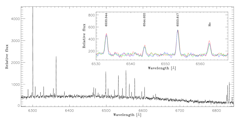
Figure 1: An example of median-resolution dark night sky spectrum. The black is the combined spectrum from three exposures. In order to show the details of the lines adjacent to H$\alpha$ in wavelength, we also show the three single exposure spectrum (red, green and blue lines, respectively) in the small window and narrow wavelength coverage.

Aiming to explore the details of H$\rm\alpha_{sky}$, such as line intensity, line dispersion, and the possible correlations with other sky lines, we carried out a special observation on 2020 November 08, that all fibers are assigned to blank sky regions instead of stars or galaxies. Besides, this plate has been set to point to a field at high Galactic altitude (l, b)= (1092, -303) to avoid the pollution of the diffuse emissions from the Galactic plane. The field has been observed for a total of 2700s, with the integration time of 900s for each one of the three exposures.

The combined spectrum in the red channel is shown in Figure 1. We can see the strongest line is Oi $\lambda$6300. Three single exposure spectra in a narrower wavelength coverage are shown with different colors in the small window. Besides H$\rm\alpha_{sky}$, there are three other OH sky lines with the wavelength in air of 6533.044, 6544.022, and 6553.617 Å, which are referred to as $\lambda$6533, $\lambda$6544 and $\lambda$6554 in the following text. We note that $\lambda$6533, $\lambda$6544, $\lambda$6554 are single lines and have been used to recalibrate the wavelength for the LAMOST-MRS-N data (Ren et al. 2021). The other reason of analyzing these lines is that they have similar wavelengths to H$\rm\alpha_{sky}$, therefore the effects of the line spread function, wavelength solution, and efficiency along the wavelength can be omitted.

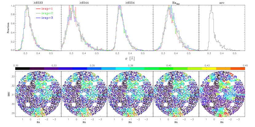
Figure 2: Top row: histograms of the line dispersions of four sky lines and that of the mean value of two arc lines. The results of the first, second and third exposure for the sky lines are plotted as red, green and blue lines, respectively. Bottom row: spatial distributions of the line dispersions.

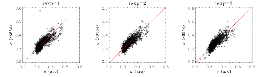
Figure 3: Comparison of the line dispersions of arc line to sky line $\lambda 6554$. The results of the first, second and third exposure are listed from left to right. The red line is the 1:1 line.

For each of these four lines, we fit it with a single Gaussian profile and obtain simultaneously line centroid, line dispersion, and line intensity. In the upper panels in the left four columns in Figure 2, we checked the histograms of line dispersions of all fibers in the field. The red, blue and green lines stands for the first, second and third exposure, respectively. For all the lines, the histograms do not change among three exposures. However, none of these histogram is a Gaussian profile, instead, there is an obvious tail at the larger line dispersion. As the sharp arc line in the Th-Ar lamp spectrum, which is used for the wavelength calibration, can be assumed to have no intrinsic broadening, the line dispersion is caused by the instrumental broadening. We show the result of the mean value of two arc lines ($\lambda$6531 and $\lambda$6584) in the right column, and found the similar distribution to the sky lines. The tails of the distributions of both sky and arc lines can be explained according to the spatial distributions shown in the bottom panels, in which there are some fibers have obvious larger line dispersions in some spectrographs. The pattern will disappear when the current problem of the consistency of fiber resolution is resolved. We should keep in mind that, if we want to study two-dimensional distribution of the velocity dispersion of the ISM, the instrumental broadening should be removed, otherwise, the intrinsic broadening from the instrument will affect the result dramatically.

We then compared the line dispersion of the arc line with the sky line $\lambda$6554 one by one in Figure 3. It is found that the line dispersion of $\lambda$6554 is identical with that of the arc line, indicating the instrumental broadening also dominates the line dispersion of the sky line $\lambda$6554. However, it is not true for H$\rm\alpha_{sky}$. As shown in Figure 4, the line dispersion of H$\rm\alpha_{sky}$ is systematically higher than that of the sky line $\lambda$6554. It is found that an extra broadening of 0.14 Å should be added to the line dispersion of $\lambda$6554 to match that of H$\rm\alpha_{sky}$. Physically, geocoronal H$\alpha$ is not a single line, instead, it is composed mainly of two single lines, with a flux ratio about 2:1 and a wavelength differ of 0.047 Å, or equally 2.133 $\rm km\,s^{-1}$ in Doppler shifts (Mierkiewicz et al. 2006). With the resolution power of 7500, we cannot resolve theses two components and a single Gaussian component can fit this line well. However, the line dispersion is higher than that of a single sky/arc line which is broadened mainly by the instrumental broadening. This extra broadening caused by the two components is about 0.02 Å, therefore the emission from the Warm Ionized Medium (WIM) and/or unresolved, faint nebulae might cause the large difference of the line dispersions between H$\rm\alpha_{sky}$ and the sky line $\lambda$6554. As revealed by the Wisconsin H$\alpha$ Mapper (WHAM) survey, this emission is present at some level over the whole sky, even at $|b|\sim 30^{\circ}$ (Nossal et al. 2001), where the dark sky plate is targeted.

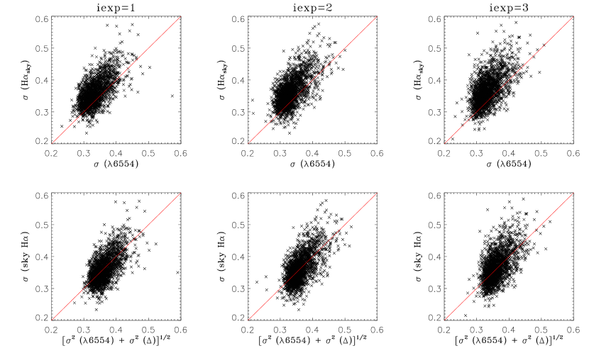
Figure 4: Top row: comparison of the line dispersion between $\lambda 6554$ and H$\rm\alpha_{sky}$. Bottom row: an extra dispersion of 0.14 Å has been added to sky $\lambda$6554 to compare to H$\rm\alpha_{sky}$. The red line is the 1:1 line.

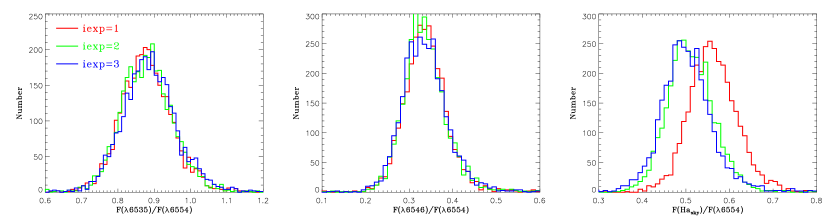
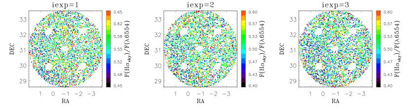
Figure 5: Top row: the histograms of $\rm F(H\alpha_{sky})/F(\lambda 6554)$ ratio. Colours stands for different exposures. Bottom row: The spatial distribution of $\rm F(H\alpha_{sky})/F(\lambda 6554)$ ratio for each single exposure.

Finally, we explored whether the F(H$\rm\alpha_{sky}$)/F($\lambda$6554) ratio changes with time. The histograms of the ratios have been shown in the upper panels in Figure 5. As can be seen, the ratios of F($\lambda$6535)/F($\lambda$6554) and F($\lambda$6544)/F($\lambda$6554) do not change with time, while the F(H$\rm\alpha_{sky})$/F($\lambda$6554) ratios from the second and third exposures change significantly compared to that from the first exposure. This result indicates that we should first derive the realistic ratio if we want to use the sky $\lambda$6554 to infer the intensity of H$\rm\alpha_{sky}$. In the bottom panels, we show the spatial distributions of the F(H$\rm\alpha_{sky})$/F($\lambda$6554) ratio, and found there is no obvious pattern or spatial gradient, indicating that a single ratio should be good enough for a whole plate to describe the H$\rm\alpha_{sky}$ component. Although the emission from the WIM and/or faint nebulae is blended with the H$\rm\alpha_{sky}$ component, the line intensity is too low to change the two-dimensional distribution in the plate (see Section 2.3).

In a summary, the H$\alpha$ sky component has a little large line dispersion compared to the sky line $\lambda$6554 which is mainly instrumental broadening, and its line dispersion can be inferred from $\lambda$6554 by adding an additional broadening of 0.02 Å. Besides, the F(H$\rm\alpha_{sky})$/F($\lambda$6554) ratio can be taken as a constant in a specific exposure. However, this ratio changes with time, we should calculate the ratio for each plate. As the science spectra in one plate are combined from three exposures, we will calculate one ratio for the plate, instead of three ratios for these exposures.

2.2 Science Spectra

Unlike the dark night sky spectrum, the H$\alpha$ emission line in science spectrum is composed of sky and nebular components. The straight way is to fit the H$\alpha$ emission using two Gaussian components. However, it cannot work well because the two components cannot always be resolved under the resolution of $R\sim 7500$. Here we define a parameter $\rm RV_{sep}$, which is the radial velocity separation between the centroids of the two components. This parameter is not determined from two-component Gaussian fit, instead, it is derived as $\rm RV_{sep}=|RV([N$ii$\rm]\lambda 6584)-RV(\lambda 6554)|$, based on the fact that $\rm RV(H\rm\alpha_{sky})\sim RV(\lambda$6554) and $\rm RV(H\alpha_{neb})\sim RV([N\,$ii]$\lambda 6584)$. We then calculate the mean value of $\rm RV_{sep}$ from its histogram in each plate, and pick out ten plates with mean $\rm RV_{sep}$ greater than $\rm 25\,km\,^{-1}$ to do further analyses. To be better describing this sample in the following text, we sort these plates according to solar altitude (sunalt) which refers to the angle of the sun relative to the Earth’s horizon, and assign ID number to them from 1 to 10. The choice of the $\rm RV_{sep}$ cut can be explained as follows. As the mean value of line dispersion of $\lambda$6554 is about 0.32 Å  (see Figure 2), the resolution power at this wavelength is about 8700 or resulting resolution of 34.5 $\rm km^{-1}$. However, we found that if we constrain the parameters as more as possible in the fitting, two components with $\rm RV_{sep}\sim 25\,km^{-1}$ still can be resolved. On the other hand, there are only several plates having $\rm RV_{sep}>34.5\,km^{-1}$, the lower cut can enlarge the analysing sample.

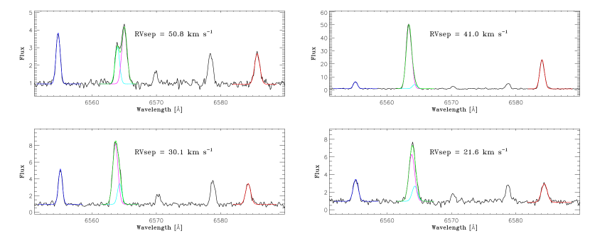
Figure 6: Four examples of fitting the H$\alpha$ emission line. Both sky $\lambda$6554 (blue) and nebular [N ii]$\lambda 6584$ (red) are fitted using a single Gaussian. The line centroid of $\rm H\alpha_{sky}$ is fixed to have same RV with $\lambda$6554, and the line dispersion is fixed to $\sqrt{\sigma(\lambda 6554)^{2}+0.02^{2}}$ Å. The line centroid of $\rm H\alpha_{neb}$ is fixed to have same RV with nebular [N ii]$\lambda$6584. The best fitting result (green) which is composed of the $\rm H\alpha_{sky}$ (cyan) and the $\rm H\alpha_{neb}$ (magenta) components is obtained by minimizing the $\chi^{2}$. The value of RV separation between the two components is indicated in each panel.

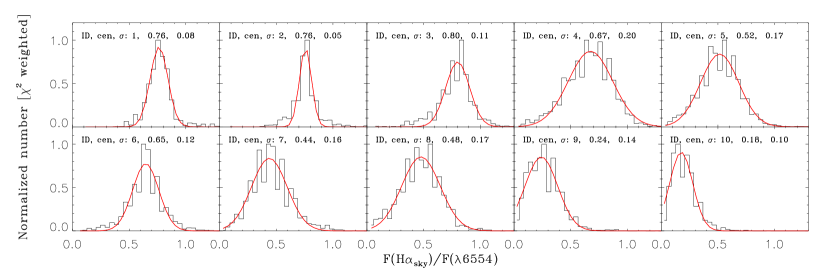
Figure 7: The histograms of F(H$\rm\alpha_{sky}$)/F($\rm\lambda$6554) ratio in ten plates. The mean value and 1$\sigma$ standard deviation of the ratio are indicated in each panel.

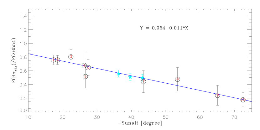
Figure 8: The $\rm F(H\rm\alpha_{sky})/F(\lambda 6554)$ ratio as a function of solar altitude. The ten plates are shown as open black circles with the ID number in the center, and have been used to fit the linear function. The three single exposures at the dark night are shown as cyan stars to make a comparison with the linear relation. The corresponding coefficients of this relation are indicated in the figure.

We show four examples of fitting the observational $\rm H\alpha$ emission lines in Figure 6. For each science spectrum, we first fit sky line $\lambda$6554 and nebular line [N ii]$\lambda$6584 using a single Gaussian, then we use the results to constrain the fitting procedure of the $\rm H\alpha$ emission line. For the H$\rm\alpha_{sky}$ component, the centroid is fixed assuming $\rm RV(H\alpha_{sky})=RV(\lambda 6554)$, the line dispersion is fixed to $\sqrt{\sigma(\lambda 6554)^{2}+0.02^{2}}$ Å, while the line intensity is set as a free parameter. For H$\rm\alpha_{neb}$, the centroid is fixed to $\rm RV(H\alpha_{neb})=RV($[N ii]$\lambda 6584)$, while the line dispersion and line intensity are set as free parameters. The best fit is obtained by minimizing the $\chi^{2}$, which is the goodness of the fit of the $\rm H\alpha$ emission line.

For each plate, we obtain the mean value of $\rm F(H\alpha_{sky})/F(\lambda 6554)$ ratio from the $\chi^{2}$-weighted histogram and corresponding 1$\sigma$ standard deviation shown in Figure 7. We can see that $\rm F(H\rm\alpha_{sky})/F(\lambda 6554)$ ratios vary from plate to plate, spanning from 0.18 to 0.83, and the 1$\sigma$ standard deviations are smaller than 0.2. This result confirms that this ratio cannot be fixed for all the plates, as we described in Section 2.1 using the dark night spectra.

2.3 Correlation between F(H$\rm\alpha_{sky}$)/F($\rm\lambda$6554) Ratio and Solar Altitude

Based on the observational data from the WHAM survey, the intensities of H$\rm\alpha_{sky}$ have been found to gradually decline with the line-of-sight shadow height (Nossal et al. 2001). As geocoronal H$\rm\alpha_{sky}$ emission mainly originates in the thermosphere and exosphere (Mierkiewicz et al. 2006), while the OH $\lambda$6554 comes from the mesopause region (Gardner et al. 2017; Xu et al. 2012), it’s expected that F(H$\rm\alpha_{sky}$)/F($\rm\lambda$6554) ratio should be correlated with solar altitude (sunalt). Because all the observations were made at night, the sunalt varies from -90 to 0 degree. We show the results derived from the ten plates in Figure 8 and find that F(H$\rm\alpha_{sky}$)/F($\rm\lambda$6554) ratio decreases with decreasing sunalt. The relation can be well fitted by a two-order polynomial function shown as blue line. The coefficients of this fitting result are indicated in the figure. We note that the three data points from the night sky field shown as filled stars are not used to the fitting. It is found that seven of ten plates follow the relation well, while the rest three plates (ID: 3, 5 and 8) slightly deviate from the relation. For the two plates (ID: 5 and 8, $\rm RV_{sep}$: 25.1 and 29.5 $\rm km\,s^{-1}$), the low $\rm RV_{sep}$ might be a possible reason of the deviation. While for the plate (ID: 3, $\rm RV_{sep}:42.8km\,s^{-1}$), the deviation might be caused by unusually activity of the sun, which may change the excitation state of atmosphere at high altitude (Kerr et al. 2001). We note that the data points from the night sky field follow the linear relation well, implying that although the WIM and/or the faint nebular line can affect the line dispersion of the H$\rm\alpha$ sky line, but the line strength of the contamination is very low compared to the sky line.

One may ask a question that how the ten plates can be representative of the whole dataset, or is there any bias to apply this relation to other plates. We here compare the parameter distributions of these ten plates to that of all 45 plates we currently have. In Figure 9 we show 45 plates as black circles in the diagrams of right ascension versus declination, azimuth versus altitude, Galactic longitude versus Galactic latitude, and ecliptic longitude versus ecliptic latitude. The seven plates which follow the relation well are shown as green filled circles, while the three plates which are slightly deviate from the relation are shown as red open circles with ID number in the center. It is found that the ten plates do not prefer special pointings. Furthermore, for each of the three “bad” plates, it has a “good” plate with a comparable parameter, except the plate ID 8 in the Galactic longitude versus Galactic latitude diagram. We then conclude that the ten plates used to derive the relation between F(H$\rm\alpha_{sky}$)/F($\rm\lambda$6554) ratio and sunalt can represent the whole dataset.

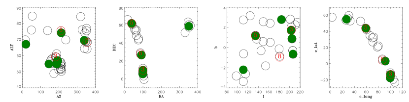
Figure 9: Parameter distributions of the observed plates. The black open circles are 45 plates we have obtained, the green filled circles are the seven plates that well follow the relation between F(H$\rm\alpha_{sky}$)/F($\rm\lambda$6554) ratio and solar altitude, while the red open circles with ID numbers are the rest three plates that slightly deviate from the relation.

2.4 Subtracting H$\rm\alpha_{sky}$ from the Science Spectrum

For each science spectrum, we first fit $\lambda$6554 with a single Gaussian, and obtain the line centroid c($\lambda 6554$), line dispersion $\sigma(\lambda 6554)$ and integrated flux F($\lambda$6554). Then we construct the H$\rm\alpha_{sky}$ component using three parameters, $\rm c(\lambda 6554)=6563/6554\times RV(\lambda 6554)$, $\rm\sigma(H\alpha_{sky})=\sqrt{\sigma(\lambda 6554)^{2}+0.02^{2}}$ Å, and $\rm F(H\alpha_{sky})=ratio\times F(\lambda 6554)$, where the ratio is the mean value in the field, which is derived from the relation shown in Figure 8. This sky component has been removed before we fit the rest spectrum using a single Gaussian. We note that during the fitting, we did not constrain the procedure anymore, instead, all the parameters are set free. In result, we obtain line centroid, line dispersion, and line intensity for the H$\alpha$ nebular component.

We then check the residual of the sky component H$\rm\alpha_{sky,residual}$ in Figure 10. In the upper two rows, we show the histogram of H$\rm\alpha_{sky}$/H$\rm\alpha_{neb}$ flux ratio. It can be seen, there is only one plate whose ratio is less than 10%, while for the rest plates the ratios can reach to about 40% or even higher. This result indicates that the sky component is necessary to be removed, otherwise the intensity of H$\alpha$ will be overestimated, and will seriously affect our analysis of the physical conditions of the ISM. In the lower two rows, we show the histograms of H$\rm\alpha_{sky,residual}$/H$\rm\alpha_{neb}$ flux ratio. It is found that, the ratios decrease significantly, and in most cases, the median value is around 0., while for the three plates (ID: 3, 5 and 8) there are a little diversion from 0 (still less than 7%), because the mean ratios derived from the relation are differ from the true situation. This result make us believe that effect of H$\rm\alpha_{sky,residual}$ to the H$\rm\alpha_{neb}$ component is less than about 10%.

We should note that, for these ten plates, we can subtract H$\rm\alpha_{sky}$ using the “true” ratio (see Figure 7). While for the other fields that RV separation is too small that the lines cannot be resolved, we will derive the ratio from the relation and remove the H$\rm\alpha_{sky}$ component. In most of cases, the residual flux is less than than 5% of the flux of H$\rm\alpha_{neb}$. Furthermore, even for the spectrum in which the sky and nebular components can be well separated, we did not try to subtract the sky component using double Gaussian fitting. Instead, we use a single value of $\rm F(H\rm\alpha_{sky})/F(\lambda 6554)$ ratio for the whole plate and subtract the sky component for each fiber according to the method described above.

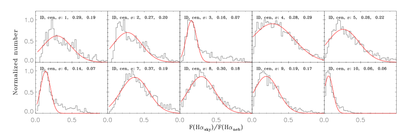
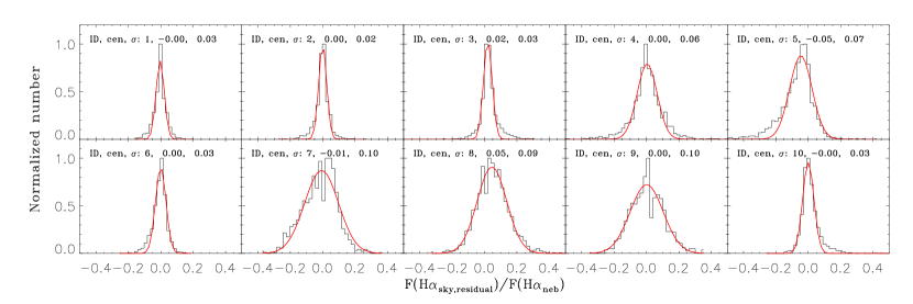
Figure 10: Upper two rows: histograms of the H$\rm\alpha_{sky}$/H$\rm\alpha_{neb}$ ratios. Bottom two rows: histograms of the ratios of H$\rm\alpha$ residual to H$\rm\alpha_{neb}$.

3 Conclusion and Discussion

Based on ten plates which the sky and nebular components can be well resolved, we investigate the correlation between H$\rm\alpha_{sky}$/$\lambda$6554 ratio and solar altitude, and develop a new method to subtract geocoronal H$\alpha$ emission from the science spectrum. The main results are summarized as follows.

• The line dispersion of OH $\lambda$6554 is mainly caused by instrumental broadening, while H$\rm\alpha_{sky}$ needs an extra broadening of 0.02 Å, because this line is composed of two single lines with different line centroids.

• The blended H$\alpha$ sky and nebular lines can be resolved by two Gaussians when the RV separation is larger than 25 $\rm km\,s^{-1}$. For this kind of plates, F(H$\rm\alpha_{sky}$)/F($\lambda$6554) ratio can be derived directly. While it is not true for the plates with RV separation smaller than 25 $\rm km\,s^{-1}$, because of the limitation of the resolution power of LAMOST-MRS-N.

• The flux ratios of the H$\alpha$ sky line to the adjacent OH $\lambda$6554 single line do not show a pattern or gradient distribution in a plate. However, we found that the ratio decreases with decreasing solar altitude, and this relation can be described by a linear function and can be used to construct the H$\rm\alpha_{sky}$ spectrum for each fiber.

• The intensity of the H$\rm\alpha_{sky}$ component seriously affect the measurements of the H$\rm\alpha_{neb}$ component. After the sky has been subtracted, the ratio of the residual of H$\rm\alpha_{sky}$ to the H$\rm\alpha_{neb}$ can be significantly down to about 10%.

There are several advantages of using the relation of geocoronal H$\alpha$ to OH $\lambda 6554$ to subtract the sky component from the science spectrum: (1) $\rm H\alpha_{sky}$ and $\lambda$6554 have very close wavelengths, hence the uncertainties caused by wavelength calibration and responding curve can be omitted. (2) OH $\lambda$6554 is a single line and is not polluted by other sky or nebular lines. (3) The line intensity of $\lambda$6554 is comparable to that of $\rm H\alpha_{sky}$. (4) Although the ratio of this two lines changes with sunalt, but the scatter of the ratio at a specific time for a plate is small.

This method is very covenient to be applied to the LAMOST-MRS-N data. For normal method, there is large uncertainties in fitting the H$\alpha$ nebular+sky line using two Gaussians when these two components have similar centroids of wavelength. Besides, it is difficult to separate the H$\alpha$ sky component from the stars with strong H$\alpha$ absorption lines, or Be, Wolf-Rayet stars with strong emission lines (Zhang et al. 2020; Wu et al. 2020), or SNRs with multi-component emissions (Ren et al. 2018). The method described in this paper is a good way to construct the H$\alpha$ sky component from the unblended sky line OH $\lambda 6554$ and subtract it from the original spectrum. The new generated spectrum is helpful to improve the accuracy of the parameters and the classifications of Galactic nebulae. Considering some plates deviate from the F(H$\rm\alpha_{sky}$)/F($\lambda$6554) – sunalt relation, we admit this method has some shortcomings. A larger sample in future is expected to find the reason of the deviation from the relation and solve this problem.

In principle, this method can be used to subtract the sky line Oi 6300 Å. However, as this line is too strong and there are no other comparable strong single sky line nearby, the uncertainty is expected to be higher than that of H$\alpha$. We will try to study this in another work.