Structured Outdoor Architecture Reconstruction
by Exploration and Classification

Abstract

This paper presents an explore-and-classify framework for structured architectural reconstruction from an aerial image. Starting from a potentially imperfect building reconstruction by an existing algorithm, our approach 1) explores the space of building models by modifying the reconstruction via heuristic actions; 2) learns to classify the correctness of building models while generating classification labels based on the ground-truth; and 3) repeat. At test time, we iterate exploration and classification, seeking for a result with the best classification score. We evaluate the approach using initial reconstructions by two baselines and two state-of-the-art reconstruction algorithms. Qualitative and quantitative evaluations demonstrate that our approach consistently improves the reconstruction quality from every initial reconstruction.

Figure 1: Our explore-and-classify reconstruction framework iterates between exploring new building structures by heuristic actions and classifying the correctness of geometries. The figure shows a particular path of exploration by our system. The red color highlights the major improvements against the previous step.

1 Introduction

Imagine a task of drawing to reconstruct the face of a person you met in the morning. This is a challenging task, where most people would perform trial and error, that is, iterate modifying and verifying the face reconstruction until being satisfied with the result. In the space of structured reconstruction, which is notoriously difficult even with the emergence of deep learning, researchers compete on designing effective neural architectures that directly reconstructs structured geometry (or its constituent information) [16, 22, 21, 24]. Our idea is to decompose the process of reconstruction into the iteration of trial and error, where the core learning is in verifying the correctness of a given geometry as opposed to one-shot geometry regression.

More concretely, the paper proposes a novel explore-and-classify approach for structured reconstruction. Starting from an imperfect building reconstruction by an existing algorithm, our approach uses simple geometry-editing actions to explore a set of offspring graphs and learns to classify the correctness of them at different levels of local geometries. At test time, we iterate exploration and classification with a search method such as beam-search or sequential Monte Carlo [6], trying to find the result with the best classification score.

We demonstrate the effectiveness of the approach on the task of structured outdoor architecture reconstruction from an aerial image [18], where a building structure is represented as a graph (See Fig. Structured Outdoor Architecture Reconstruction by Exploration and Classification). We use two baselines and two state-of-the-art algorithms [22, 18] to generate the initial reconstructions. Our system consistently makes big improvements over all the initial reconstructions and achieves state-of-the-art performance.

In summary, the contributions of this paper are two-fold: 1) A novel explore-and-classify framework with local geometry classifiers for a structured reconstruction problem; and 2) A state-of-the-art performance on outdoor architecture reconstruction problem with significant improvements over all the baselines and the best existing approaches. While we focus on one problem setting, the ideas are potentially applicable to many other structured reconstruction tasks and could further improve the performance of their state-of-the-arts. Our code and pretrained models are available at https://github.com/zhangfuyang/search_evaluate. The data is publicly available through our prior project [18].

2 Related Work

In this section, we review related work in the field of structured geometry reconstruction.

Traditional methods. Birchfield and Tomasi had a seminal paper on piecewise affine surface reconstruction, which iterates plane segmentation and affine parameter estimation [2]. The development of graphical model inference techniques such as graph-cuts [13], alpha-expansion [14], and message passing [12] enabled effective optimization algorithms for piecewise smooth depthmap reconstruction [8, 9], which produces a consistent 3D planes under the Manhattan constraint. However, they were not robust enough for production applications due to the use of many heuristics and unstable depth estimation.

Arrival of deep learning. The emergence of deep neural networks (DNNs) has brought many breakthroughs. Instance segmentation networks [10] in recognition were utilized for single-view piecewise planar depthmap reconstruction [17]. A metric learning approach for instance segmentation has also been proven effective for the same task [21]. Recurrent neural networks [3, 1] or iterative refinement approaches are utilized for polygonal curve extraction [5]. However, these approaches are segmentation methods where the region boundary is a dense set of points.

For reconstruction of CAD-level geometry with compact surface representation, a popular approach is to utilize DNNs for low level geometry inference (e.g., corner or edge detection) and optimization-based methods use heuristics to reconstruct high level topological structure [16, 4, 18].

End-to-end neural architecture for structured geometry reconstruction also exists, albeit more challenging. Convolutional graph neural networks are proposed for a 2D planar graph reconstruction given corners [22]. For wire-frame parsing of architectural scenes, end-to-end systems combine junction detection and edge verification [24] or junction detection and adjacency matrix inference [23].

Despite continued progress in neural architecture research, the task of CAD-quality geometry reconstruction is still a challenge, where state-of-the-art algorithms produce reconstructions that immediately look “wrong” to our eyes.

Reinforcement learning. Deep reinforcement learning (DRL) is an interesting way to tackle structured geometry reconstruction. Ellis et al. [7] proposed a neural program synthesis algorithm, one of whose applications is constructive solid geometry reconstruction from a 2D or 3D occupancy grid. Lin et al. [15] proposed a system that takes a depthmap and recovers a set of primitives and refines corner locations. DRL sounds elegant but requires many tricks and heuristics, notably pseudo supervised training data generation by domain-specific knowledge. Sec. 5.2 explains that our system is a special case of DRL in a simpler form while standard DRL features are not effective for structured geometry reconstruction. Our experiments show that our system makes significant improvements over the state-of-the-art DRL based reconstruction methods.

3 Problem review

The paper tackles a structured architecture reconstruction problem by Nauata et al. [18]. An input is a cropped and rescaled (i.e., 256$\times$256) aerial photograph of a building. The task is to reconstruct the building architecture as a 2D planar graph including all internal feature edges.

Suppose there exists an L shaped building consisting of two rectangular components (See the right). The output must have two T-junctions and five L-junctions with the shared internal edge.

We use the same metrics for evaluation as in Nauata et al. [18], namely f1 scores of corner, edge, and region primitives. The dataset contains 2,001 buildings. We randomly split the data into 1601 training, 50 validation, and 350 testing data. Hyper-parameters such as score weights, search depth and search width are fine-tuned on the validation set. We report all result on the test set. Note that an aerial photograph suffers from perspective distortions, where the Manhattan assumption does not always hold, yielding a very challenging structured reconstruction problem.

4 Explore-and-classify reconstruction

Figure 2: System overview. The geometry exploration module starts from an initial model reconstructed by another algorithm, and produces a set of offspring reconstructions by heuristic actions. The geometry classification module ranks the generated reconstructions and keep the top samples for the next iteration (graphs with green color score on the right corner are the top samples in each iteration). The system dynamically generates training data for the classification module by picking generated reconstructions and creating classification labels based on the ground-truth. The classification module consists of three local primitive classifiers (i.e., junctions, edges, and regions). The first two classifiers are neural networks, which learns to classify if each primitive in the current reconstruction is correct or incorrect. The region classifier measures the consistency with the instance segmentation masks generated by Mask R-CNN [10]. The overall classification score is the sum of junction, edge, and region scores.

Our idea is to decompose the process of reconstruction into the iteration of exploration and classification, where the core learning happens in classifying the correctness of a geometry (see Fig. 2).

4.1 Geometry exploration

The exploration module takes a building graph and produces a set of offspring-graphs by heuristic actions. We use the geometry classification module to rank the offspring, shrink the population (e.g., keeping top-k), and repeat the iteration of exploration and classification. The exact procedure slightly differs during testing and training. We now explain 1) the heuristic actions, 2) the test-time exploration, and 3) the training-time exploration.

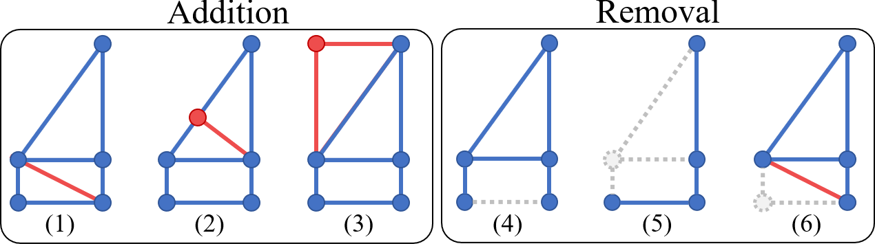
Figure 3: Heuristic actions for geometry modification. Red and grey colors indicate the added and deleted elements respectively.

Heuristic actions. The heuristic actions either add primitives or remove primitives (See Fig. 3). There are three addition actions: 1) Add an edge between a pair of existing corners; 2) Add an edge starting from a corner orthogonally towards another edge and insert a new corner at the intersection (if the intersection is outside, we extend the edge until the intersection point); 3) At two edges sharing a corner, complete a parallelogram by adding one corner and two edges. There are three removal actions: 4) Remove an edge; 5) Remove a corner and its incident edges; 6) For a degree-2 corner, remove itself and connect its end-points, which is effective for removing a colinear corner.

Test-time exploration. Given a set of building graphs, we apply every possible action to every graph, evaluate the scores based on the classifiers (See Sec. 4.2), and subsample the population using Beam search or Sequential Monte Carlo (SMC) [6]. The process repeats for a certain number of times and the graph with the highest classification score becomes the output. Our default choice is the Beam search with (depth=12, width=5), while we increase the depth to 20 or 30 depending on the quality of the initial reconstructions. See Sec. 5 for details.

Training-time exploration. During training, there is no need to seek for the best reconstruction for each sample, and we favor population diversity and efficiency. We take one action for each of the 6 action types for each graph. For example, an edge removal action is applied to one edge with a uniform probability. In each iteration, we keep the top two graphs based on the classification scores, while using an epsilon-greedy strategy to replace one with a random graph with 20% chance.

Overall, starting from each training building, we generate 12(=6$\times$2) candidate graphs per iteration (6 in the first iteration), and repeat for 5 times. The top 2 graphs (w/ random replacement) at each of the five iterations, that is, 10 building graphs are added to the training set. See Sec. 4.2 for the classification label generation.

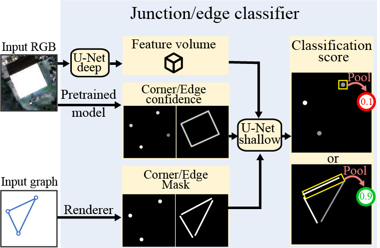
Figure 4: Junction/edge classifier. The architecture consists of two U-Net models (U-Net deep and U-Net shallow). U-Net deep transforms an input image into a feature volume. U-Net shallow takes the feature volume, a corner/edge confidence image generated by a pre-trained CNN, and a corner/edge mask image rasterized from the current graph as the input. It then produces a pixel-wise classification score. We use average pooling among pixels over a primitive to compute the final classification score for each primitive.

4.2 Geometry classification

We define three levels of geometric primitives in a building graph, namely junctions $\mathcal{J}$=$\{j\}$, edges $\mathcal{E}$=$\{e\}$, and regions $\mathcal{R}$=$\{r\}$. Note that a junction is a corner with information of the incident edge angles and a region is a 2D polygon surrounded by a set of edges. Our geometry classification learns to classify the correctness of each geometric primitives. The classification score is:

$$w_{j}\underset{j\in\mathcal{J}}{\sum}C_{\text{junc}}(j)+w_{e}\underset{e\in\mathcal{E}}{\sum}C_{\text{edge}}(e)+w_{r}C_{\text{region}}(\underset{r\in\mathcal{R}}{\cup}r).$$ (1)

$C_{\text{junc}}(j)$ and $C_{\text{edge}}(e)$ are the junction/edge classification scores. $C_{\text{region}}(r)$ is the region score. The range of $C_{\text{junc}}$, $C_{\text{edge}}$ and $C_{\text{region}}$ are $[-1,1]$, $[-1,1]$, and $[0,1]$ respectively. Junction and edge classification scores are summed over the primitive instances. Region score is evaluated for the union of all the region instances. $w_{j,e,r}$ are the scaling weights. We now go over the details.

Junction/edge classifiers. We use the same architecture for the junction and edge classifiers. Their inputs are the aerial image and a building graph, and the output is pixel-wise classification scores.

The classifier consists of two U-Nets (See Fig. 4). The first “deep U-Net” is responsible for extracting global building feature volumes. At test time, deep U-Net runs only once for each building image, significantly reducing the computational expenses. The second “shallow U-Net” (half resolution and 1 less layer) is responsible for producing the pixel-wise classification scores as an image. The input is the feature volume, corner/edge confidence images as in Nauata et al. [18], and the corner/edge binary segmentation masks, rasterized from the current building graph (3 pixels of diameters for corners and 2 pixels of thickness for edges).

We take the score at a corner pixel as the corner classification score $C_{\text{junc}}$, and take the average over the pixels along an edge as the edge classification score $C_{\text{edge}}$. See the supplementary document for the full architecture details.

Region classifier. A natural extension of the junction/edge classifiers to region is to label each region instance as correct/incorrect and train a similar classifier. However, such an approach degraded performance. We found that this is due to the ambiguity in the annotations. Suppose a system reconstructs a building with two regions in the image below, but the annotation is a single region (w/o the orange structure). All the regions will have small IoU against ground-truth and become incorrect. On the other hand, influences to the junction/edge classifiers are smaller: only 2 out of 9 junctions and

3 out of 10 edges become incorrect. Therefore, we define our region score to be the IoU metric between the union of all the regions against the union of instance segmentations obtained by a pretrained Mask R-CNN [10].

Classification label generation. For the initial reconstructions and new training samples generated by the exploration, we use the ground-truth to generate classification labels. First, we establish corner-to-corner correspondences by greedily matching the closest pair within 7 pixels in distance, where no two corners can match to same GT corner. A junction is labeled as correct if it matches with a GT corner and their incident edge directions are the same with an error tolerance of 10 degrees. An edge is labeled as correct if its end-points match with two corners that are also connected in GT.

Loss function. The raw output of junction/edge classifiers are pixel-wise scores in the range [-1, 1]. The ground-truth is set to (1, 0, -1) for the pixels over (positive-primitives, background, negative-primitives), where corner and edge primitives are rasterized with 3 pixels of diameters and 2 pixels of thickness, respectively. We enforce pixel-wise Huber loss ($\delta=1.0$) of the output from junction/edge classifiers against the ground-truth. The weight of the loss is set to half for the background pixels.

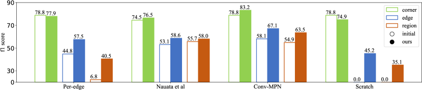
Figure 5: Quantitative evaluations. Two baselines (Per-edge and Scratch) and two state-of-the-art algorithms (Nauata et al. and Conv-MPN) are used to generate initial reconstructions to run our system. Corner, edge and region f1 scores are shown in different colors. Empty and solid bars refer to original and our reconstructions. Our system makes consistent improvements in almost all cases.

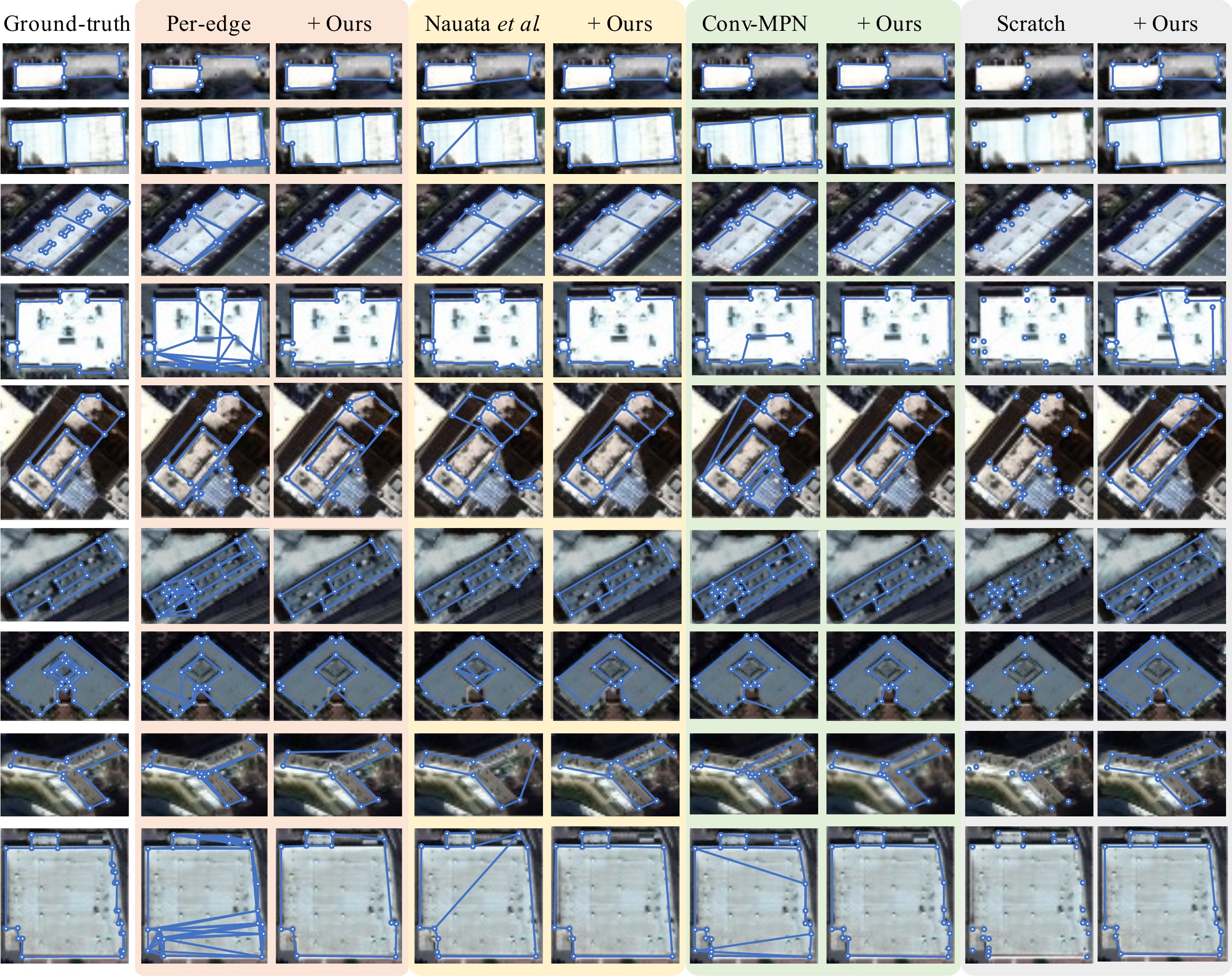
Figure 6: Qualitative evaluations. Improvements are also qualitatively clear in every case. Refer to the supplementary for more examples.

5 Experiments

We implement the system in PyTorch [19] and use a workstation with Xeon CPU (20 cores) and dual Titan RTX. Training is divided into pre-training and fine-tuning phases. In the pre-training phase, initial reconstructions by an existing algorithm are used as training samples and train for 90 epochs. The fine-tuning phase runs with 2 threads. The first thread conducts exploration while producing more training samples. The second thread fine-tunes the classifiers for 20 epochs. The networks weights of the classifiers are updated by the second thread after each epoch, which is used by the first thread for the exploration. Approximately, 1200 more training samples are generated in each epoch.

During pre-training, learning rate starts from $5\times 10^{-4}$ and is reduced by half every 30 epochs. During fine-tuning, learning rate starts from $2\times 10^{-4}$ and is reduced by half every 5 epochs. In all our experiments, we use the Adam optimizer [11] with a batch-size of 16. Training takes 8 hours on average. During testing, running time depends on the search width and depth. Default setting of width=5, depth=12 takes around 3 to 4 hours for 350 test buildings.

5.1 Main results

Our system works with any reconstruction algorithms that produce the initial graphs. We test 2 baselines and 2 state-of-the-art algorithms, where the four experiments are conducted independently without mixing training samples.

Per-edge classifier is the first baseline, which classifies correctness of every edge given building corners from a CNN. See the supplementary document for the details.

Nauata et al. [18] is the first state-of-the-art algorithm, which relies on integer programming with heuristic objectives. We use the official implementation.

Conv-MPN [22] is the second state-of-the-art, which use an end-to-end graph neural network to classify the correctness of each edge candidate. We use the official implementation.

Scratch is an extreme case where we only use corners detected by a standard CNN without any edges. A corner detector from the Conv-MPN system is used. We allow only addition actions in the first 10 steps at training and testing.

We use a simple grid search with the validation set to find the best hyperparameters. Scaling weights for the three classification scores (junction, edge, region) in Eq. 1 are (1, 2, 50) for Per-edge and Conv-MPN, and (1, 1, 50) for Nauata et al. and Scratch. The search depth and width are (12, 5) for Nauata et al. and Conv-MPN. Per-edge and Scratch requires more exploration and use (20, 5) and (30, 8).

Fig. 5 is our quantitative result, comparing corner, edge, and region f1 scores between initial and our reconstructions. The proposed approach consistently improves the edge and the region metrics in every single case. The corner metric degrades in the case of Per-edge and Scratch. However, as shown in Fig. 6, the corner metric at the lowest level primitive does not capture the overall reconstruction quality. Original reconstruction by Per-edge and scratch suffer from various artifacts such as dangling edges, overlapping edges, and unlikely structure as a building, all of which are handled well by our system. Even in the extreme case Scratch, our system removes noisy corners and adds meaningful edges to recover most building structure.

While our system does its best in improving original reconstructions, the final quality depends on the initial models. Our system achieves the best performance with Conv-MPN but performs worse with Scratch, which is simply because Scratch requires more actions towards a good reconstruction, making the search space exponentially larger.

5.2 Comparison with Reinforcement Learning

Reinforcement learning (RL) is an interesting way to tackle structured geometry reconstruction. We compare against two state-of-the-art RL based structured reconstruction systems, Ellis et al.  [7] and Lin et al.  [15].

Algorithm comparison. Ellis et al. proposed a neural program synthesis algorithm, one of whose applications is constructive solid geometry reconstruction from occupancy grid. Lin et al. proposed a system that manipulates a set of primitives to reconstruct a 3d shape. We adapt the implementation of our system to reproduce their works. For both systems, a state is a corner/edge mask image together with the aerial image. An action is represented by the corner/edge mask difference between the current and the next states. The action set is the same as ours. A reward function is based on the entire graph and dependent on the action. We want to assess only the core RL system components and remove the imitation learning in Lin et al. and the pre-training in Ellis et al. . The following are more details.

$\bullet$ REPL trains a policy network with REINFORCE where reward is 1 for the last state if classification score is within 8.0 from that of the ground-truth, and 0 otherwise. A state value function is also trained based on the reward. We follow their optimization procedure to train the two models with $\gamma$=1 while sampling actions with the policy network. Sequential Monte Carlo is used at test time.

$\bullet$ Lin et al. originally defines the reward as increase in IoU score between current state and target state. Similarly, we define the reward as an increase in the classification score after each action. Reward discount factor is set to the same 0.9. We train a double DQN [20] following their procedure.

Reduction to RL. Our system is a special case of temporal difference reinforcement learning (TD-RL) for state value function, whose general formula is

$$V^{\pi}(s)=\mathbb{E}_{\pi}\left[R(s,a)+\gamma V^{\pi}(s^{\prime})|s\right].$$ (2)

$s$ is the current state and $s^{\prime}$ is the next state after an action $a$ with reward $R(s,a)$. $\gamma$ and $V$ denote a discount factor and a state value function. $\pi$ is the policy. Our classifiers evaluate goodness of a reconstruction and are equivalent to the value function. Classification labels are based on ground-truth and are equivalent to the reward. Three specializations reduce the TD-RL formulation into our approach: (1) setting $\gamma=0$ to ignore future rewards, (2) making reward solely depends on the state, and (3) Per primitive classifiers design instead of a single function evaluating the goodness of the entire state [7, 15]. (1) and (2) reduce Eq. 2 to $V(s)=R(s)$, where $R(s)$ is the classification labels in our case. (3) breaks reward down to local primitives. We have $V(\tilde{s})=R(\tilde{s})$ for each geometric primitive $\tilde{s}$, which exactly matches our formulation in Sec. 4.2.

Table 1: Comparison against two state-of-the-art RL-based systems, Ellis et al. and Lin et al. based on the corner/edge/region f1 scores. All systems use Conv-MPN reconstructions as the initial models. orange and cyan indicate best and second best scores.

Algorithm	Corner	Edge	Region
Conv-MPN [22]	78.8	58.1	54.9
REPL [7]	72.6	43.8	15.9
Lin et al.  [15]	74.7	51.6	35.8
+ Ours	83.2	67.1	63.5

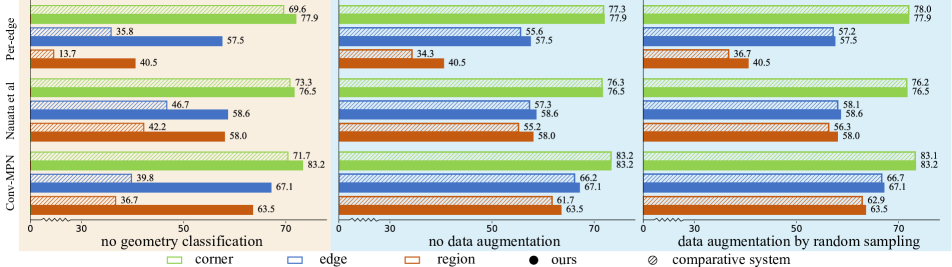
Figure 7: Ablation studies: (Left) The geometry classifier is replaced by a simple heuristic rule based on the corner/edge confidence map (an input to the classifier, see Fig. 4). This version does not require any training and merely performs explore-and-classify by heuristic rules. (Right) Data augmentation by the exploration module is replaced by no augmentation or random sampling. Each study reports numbers with three different initial reconstruction algorithms.

Empirical comparisons. Table 1 is the quantitative comparison of two RL based methods with ours, where Conv-MPN is the initial reconstructions for all the three systems. It is a surprise that Ellis et al. and Lin et al. rather make the results worse from the original Conv-MPN reconstructions. This shows the limitation of using RL on the structured data, which fails to learn patterns in architectural geometry and rather become a noisy guidance damaging the reconstruction.

Figure 8: Ablation study on the effectiveness of exploration module. We show the performance gap between ours and no data augmentation. The top (resp. bottom) row shows the corner/edge/region f1 scores when using Per-edge (resp. Nauata et al. ) as the initial reconstructions. The performance gap grows as search depth increases, because data augmentation becomes more effective as reconstruction samples differ more from the originals.

5.3 Ablation studies

We verify the contributions of each individual components in our system together with the assessment on the generalization capability.

Exploration module. Our exploration module collects training data dynamically by utilizing the classification module. We experiment two ablation approaches for the training data collection. The first one denoted as no data augmentation, which does not explore and simply use the initial reconstructions as the only training data. The second one denoted as data augmentation by random sampling, which uses random sampling instead of our classifiers to perform exploration and select training samples. Fig. 7 shows that both two ablation approaches are inferior to our exploration module with an exception of one entry in the corner metric with Per-edge initial reconstruction, which is not a good reflection of overall reconstruction quality as discussed in Sec. 5.1. For both no data augmentation and data augmentation by random sampling, the region metric gap with ours is larger when initial reconstructions are of low quality (i.e. Per-edge).

Fig. 8 further shows that the performance gap between no data augmentation and our exploration module grows as the search depth increases. This agrees with our intuition that the data augmentation is more effective when building models differ more from the initial reconstructions.

Classification module. To verify the effectiveness of the junction/edge classifiers, we replace them with a heuristic method based on the corner/edge confidence images utilized inside the classifiers (See Fig. 4). Concretely, we simply use the corner/edge confidence images for pooling, instead of the pixel-wise classification scores. The rest of the pipeline stays the same. Fig. 7 shows that the lack of classification module significantly degrades the performance, in fact, made the results even worse than the initial reconstructions.

Search strategy. Sequential Monte Carlo [6] (SMC) is another popular search method. We replace Beam search with SMC at test time, sampling 5 graphs based on the classification scores at each iteration and repeat for 12 times (our default search depth). Table 2 compares SMC against Beam search while using Conv-MPN as the initial reconstructions. Our system achieves clear improvements over the original reconstructions in both cases.

Generalization capability. We evaluate the generalization capability of our approach across different initial reconstructions based on the corner/edge f1 scores in Table. 3. For example, the value of 76.6 in the second column indicates a score when Conv-MPN [22] is used at training and Nauata et al.  [18] is used at testing. Our system is able to achieve high performance regardless of the training/testing data combination. One interesting discovery is the right most column where Per-edge reconstructions are used at test-time. It is a surprise that using Conv-MPN or Nauata et al. at training is better. Our hypothesis is that reconstructions by Conv-MPN or Nauata et al. contain both high quality local geometries (close to GT) as well as poor local geometries (i.e., reconstruction failures), enabling the classifiers to learn from a diverse set of training samples. On the other hand, Per-edge reconstructions are mostly poor as indicated by the original f1 scores, making it difficult for the classifiers to learn diverse scenarios.

Table 2: Our system works well with different search algorithms.

Algorithm	Corner	Edge	Region
Beam search	83.2	67.1	63.5
SMC [6]	81.2	65.6	64.0

Table 3: Assessing generalization capability across different initial reconstructions. Columns and rows indicate the initial reconstructions at testing and training time, respectively. (corner/edge) f1 scores are reported in the table. The third row (labeled Original) shows the f1 scores of the original reconstructions by the three systems as a reference.

	Test-time initialization
	Conv-MPN	Nauata et al.	Per-edge
Original	78.8 / 58.1	74.5 / 53.1	78.8 / 44.8
Conv-MPN	83.2 / 67.1	76.6 / 58.5	81.1 / 60.3
Nauata et al.	83.1 / 67.0	76.5 / 58.6	80.5 / 60.1
Per-edge	82.7 / 65.4	75.0 / 56.0	77.9 / 57.5

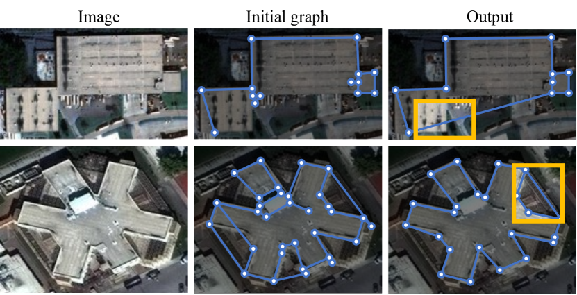
Figure 9: Failure modes. The top row shows an example suffering from missing corners. The bottom row shows a complex building with weak image signal.

5.4 Limitations

While the proposed system achieves the best performance over the competing state-of-the-art with a clear margin, there are a few limitations. First, test-time inference is slow, which is a general limitation for any search based methods. Next, The system also has a few major failure modes (See Fig. 9). The first mode comes from missing corners. Corner addition is a challenging action with many degrees of freedom. Our system fails to recover from extreme corner detection failures, e.g. a region misses multiple corners. The second mode comes from the classification mistake when the image signal is weak. Our CNN-based classifiers are inferior to the human vision system in analyzing the consistency of structured geometry and an image.

6 Conclusion

This paper presents a novel explore-and-classify framework for structured outdoor architecture reconstruction, seeking to improve the quality of imperfect building reconstructions. Our system learns to classify the correctness of primitives while exploring the space of reconstructions via heuristic actions. Qualitative and quantitative evaluations demonstrates significant improvements over all state-of-the-art methods. While we verify the effectiveness of our idea on one particular reconstruction task, the computational framework is general. We believe that the ideas are potentially applicable to many other structured reconstruction tasks and beyond.

Acknowledgement. This research is partially supported by NSERC Discovery Grants with Accelerator Supplements and DND/NSERC Discovery Grant Supplement.

References

- [1] David Acuna, Huan Ling, Amlan Kar, and Sanja Fidler. Efficient interactive annotation of segmentation datasets with polygon-rnn++. In Proceedings of the IEEE conference on Computer Vision and Pattern Recognition, pages 859–868, 2018.
- [2] Stan Birchfield and Carlo Tomasi. Multiway cut for stereo and motion with slanted surfaces. In Proceedings of the seventh IEEE international conference on computer vision, volume 1, pages 489–495. IEEE, 1999.
- [3] Lluis Castrejon, Kaustav Kundu, Raquel Urtasun, and Sanja Fidler. Annotating object instances with a polygon-rnn. In Proceedings of the IEEE conference on computer vision and pattern recognition, pages 5230–5238, 2017.
- [4] Jiacheng Chen, Chen Liu, Jiaye Wu, and Yasutaka Furukawa. Floor-sp: Inverse cad for floorplans by sequential room-wise shortest path. In Proceedings of the IEEE/CVF International Conference on Computer Vision, pages 2661–2670, 2019.
- [5] Dominic Cheng, Renjie Liao, Sanja Fidler, and Raquel Urtasun. Darnet: Deep active ray network for building segmentation. In Proceedings of the IEEE/CVF Conference on Computer Vision and Pattern Recognition, pages 7431–7439, 2019.
- [6] Arnaud Doucet, Nando De Freitas, and Neil Gordon. An introduction to sequential monte carlo methods. In Sequential Monte Carlo methods in practice, pages 3–14. Springer, 2001.
- [7] Kevin Ellis, Maxwell Nye, Yewen Pu, Felix Sosa, Josh Tenenbaum, and Armando Solar-Lezama. Write, execute, assess: Program synthesis with a repl. arXiv preprint arXiv:1906.04604, 2019.
- [8] Yasutaka Furukawa, Brian Curless, Steven M Seitz, and Richard Szeliski. Manhattan-world stereo. In 2009 IEEE Conference on Computer Vision and Pattern Recognition, pages 1422–1429. IEEE, 2009.
- [9] David Gallup, Jan-Michael Frahm, and Marc Pollefeys. Piecewise planar and non-planar stereo for urban scene reconstruction. In 2010 IEEE Computer Society Conference on Computer Vision and Pattern Recognition, pages 1418–1425. IEEE, 2010.
- [10] Kaiming He, Georgia Gkioxari, Piotr Dollár, and Ross Girshick. Mask r-cnn. In Proceedings of the IEEE international conference on computer vision, pages 2961–2969, 2017.
- [11] Diederik P Kingma and Jimmy Ba. Adam: A method for stochastic optimization. arXiv preprint arXiv:1412.6980, 2014.
- [12] Vladimir Kolmogorov. Convergent tree-reweighted message passing for energy minimization. IEEE transactions on pattern analysis and machine intelligence, 28(10):1568–1583, 2006.
- [13] Vladimir Kolmogorov and Ramin Zabih. Multi-camera scene reconstruction via graph cuts. In European conference on computer vision, pages 82–96. Springer, 2002.
- [14] Vladimir Kolmogorov and Ramin Zabin. What energy functions can be minimized via graph cuts? IEEE transactions on pattern analysis and machine intelligence, 26(2):147–159, 2004.
- [15] Cheng Lin, Tingxiang Fan, Wenping Wang, and Matthias Nießner. Modeling 3d shapes by reinforcement learning. In European Conference on Computer Vision, pages 545–561. Springer, 2020.
- [16] Chen Liu, Jiajun Wu, Pushmeet Kohli, and Yasutaka Furukawa. Raster-to-vector: Revisiting floorplan transformation. In Proceedings of the IEEE International Conference on Computer Vision, pages 2195–2203, 2017.
- [17] Chen Liu, Jimei Yang, Duygu Ceylan, Ersin Yumer, and Yasutaka Furukawa. Planenet: Piece-wise planar reconstruction from a single rgb image. In Proceedings of the IEEE Conference on Computer Vision and Pattern Recognition, pages 2579–2588, 2018.
- [18] Nelson Nauata and Yasutaka Furukawa. Vectorizing world buildings: Planar graph reconstruction by primitive detection and relationship inference. In European Conference on Computer Vision, pages 711–726. Springer, 2020.
- [19] Adam Paszke, Sam Gross, Francisco Massa, Adam Lerer, James Bradbury, Gregory Chanan, Trevor Killeen, Zeming Lin, Natalia Gimelshein, Luca Antiga, et al. Pytorch: An imperative style, high-performance deep learning library. arXiv preprint arXiv:1912.01703, 2019.
- [20] Hado Van Hasselt, Arthur Guez, and David Silver. Deep reinforcement learning with double q-learning. In Proceedings of the AAAI Conference on Artificial Intelligence, volume 30, 2016.
- [21] Zehao Yu, Jia Zheng, Dongze Lian, Zihan Zhou, and Shenghua Gao. Single-image piece-wise planar 3d reconstruction via associative embedding. In Proceedings of the IEEE/CVF Conference on Computer Vision and Pattern Recognition, pages 1029–1037, 2019.
- [22] Fuyang Zhang, Nelson Nauata, and Yasutaka Furukawa. Conv-mpn: Convolutional message passing neural network for structured outdoor architecture reconstruction. In Proceedings of the IEEE/CVF Conference on Computer Vision and Pattern Recognition, pages 2798–2807, 2020.
- [23] Ziheng Zhang, Zhengxin Li, Ning Bi, Jia Zheng, Jinlei Wang, Kun Huang, Weixin Luo, Yanyu Xu, and Shenghua Gao. Ppgnet: Learning point-pair graph for line segment detection. In Proceedings of the IEEE/CVF Conference on Computer Vision and Pattern Recognition, pages 7105–7114, 2019.
- [24] Yichao Zhou, Haozhi Qi, and Yi Ma. End-to-end wireframe parsing. In Proceedings of the IEEE/CVF International Conference on Computer Vision, pages 962–971, 2019.