The Generalized Gamma distribution as a useful RND under Heston’s stochastic volatility model

Abstract

Following Boukai (2021) we present the Generalized Gamma (GG) distribution as a possible RND for modeling European options prices under Heston’s (1993) stochastic volatility (SV) model. This distribution is seen as especially useful in situations in which the spot’s price follows a negatively skewed distribution and hence, Black-Scholes based (i.e. the log-normal distribution) modeling is largely inapt. We apply the GG distribution as RND to modeling current market option data on three large market-index ETFs, namely the SPY, IWM and QQQ as well as on the TLT (an ETF that tracks an index of long term US Treasury bonds). The current option chain of each of the three market-index ETFs shows of a pronounced skew of their volatility ‘smile’ which indicates a likely distortion in the Black-Scholes modeling of such option data. Reflective of entirely different market expectations, this distortion appears not to exist in the TLT option data. We provide a thorough modeling of the available option data we have on each ETF (with the October 15, 2021 expiration) based on the GG distribution and compared it to the option pricing and RND modeling obtained directly from a well-calibrated Heston’s (1993) SV model (both theoretically and empirically, using Monte-Carlo simulations of the spot’s price). All three market-index ETFs exhibit negatively skewed distributions which are well-matched with those derived under the GG distribution as RND. The inadequacy of the Black-Scholes modeling in such instances which involve negatively skewed distribution is further illustrated by its impact on the hedging factor, delta, and the immediate implications to the retail trader. In contrast, for the TLT ETF, which exhibits no such distortion to the volatility ‘smile’, the three pricing models (i.e. Heston’s, Black-Scholes and Generalized Gamma) appear to yield similar results.

Keywords: Heston model, option pricing, risk-neutral valuation, calibration, volatility skew, negatively skewed distribution, SPY, QQQ, IWM, TLT.

1 Introduction

One of the most widely celebrated option pricing model for equities (and beyond) is that of Black and Scholes (1973) and of Merton (1973), (abbreviated here as the BSM). Their option pricing model was derived under some simple assumptions concerning the distribution of the asset’s returns, coupled with presumptive continuous hedging, self-financing, zero dividend, risk-free interest rate, $r$, and no cost of carry or transactions fees. In its standard form, the BSM model assumes that the spot’s price process ${\cal{S}}=\{S_{t},\,t\geq 0\}$ evolves with a constant volatility of the spot’s returns, $\sigma$, as a geometric Brownian motion (under a risk-neutral probability measure $\mathbb{Q}$, say), leading to an exact solution for the price, $C(\cdot)$, of an European call option. Specifically, given the current spot price $S_{\tau}=S$ and the risk-free interest rate $r$, the price of the corresponding call option with price-strike $K$ and duration $T$,

$$C_{S}(K)=S\,\Phi(d_{1})-K\,e^{-rt}\,\Phi(d_{2}),$$ (1)

where $t=T-\tau$ is the remaining time to expiry. Here, we use the conventional notation to denote by $\Phi(\cdot)$ and $\phi(\cdot)$ the standard Normal cumulative distribution function ($cdf$) and density function ($pdf$), respectively, and where

$$d_{1}:=\frac{-\log(\frac{K}{S})+(r+\frac{\sigma^{2}}{2})t}{\sigma\sqrt{t}}\qquad\text{and}\qquad d_{2}:=d_{1}-\sigma\sqrt{t}.$$ (2)

Despite of its wide acceptability in the retail trading world this model hinges on several incorrect assumptions and hence, suffers from some notable deficiencies; see for example Black (1988, 1989) who pointed out the holes in Black-Scholes. Chief among the noted deficiencies is the fact that volatility of spot’s returns (i.e., $\sigma$) appears not to be constant over the ‘life’ of of the option, but rather varying at random.

The efforts to incorporate a non-constant volatility in the option valuation (e.g., Wiggins (1987) or Stein and Stein (1991)) has culminated with Heston’s (1993) stochastic volatility (SV) model. This SV model incorporates, aside from the dynamics of the spot’s price process ${\cal{S}}$, also the dynamics of a corresponding, though unobservable (hence untradable), volatility process ${\cal{V}}=\{V_{t},\,t\geq 0\}$. Instructed by the form of the exact BSM solution in (1), Heston (1993) obtained that the solution to the system of PDE he obtained from the stochastic volatility model he constructed is given by

$$C_{S}(K)=S\,P_{1}-K\,e^{-rt}\,P_{2},$$ (3)

where $P_{j}$ $j=1,2$, are two related (under $\mathbb{Q}$) conditional probabilities that the option will expire in-the-money, conditional on the given current stock price $S_{\tau}=S$ and the current volatility, $V_{\tau}=V_{0}$. However, unlike the explicit BSM solution in (1) which is given in terms of the normal (or log-normal) distribution, Heston (1993) provided (semi) closed-form solutions to these two probabilities, $P_{1}$ and $P_{2}$, both given in terms of their characteristic functions. These characteristic functions depend on some parameters of the SV model, $\vartheta=(\kappa,\theta,\eta,\rho)$ and may be numerically evaluated, via complex integration, for any choice of the parameters $\vartheta$ in addition to the given $S,\ V_{0}$ and $r$ (for more details, see the Appendix). The components of $\vartheta$ have particular meaning in context of Heston’s (1993) SV model: $\rho$ is the correlation between the random components of the spot’s price and volatility processes, ; $\theta$ is the long-run average volatility, $\kappa$ is the mean-reversion speed for the volatility dynamics and $\eta^{2}$ is the variance of the volatility $V$. It should be noted that different choices of $\vartheta$ will lead to different values $C_{S}(K)$ in (3) and hence, the value ${\vartheta}=(\kappa,\theta,\eta,\rho)$ must be appropriately ‘calibrated’ first for $C_{S}(K)$ to actually match the option market data. However, this calibration process typically involves substantial numerical challenges (resulting from the complex-domain integration and the required multi-dimensional optimization) and in light of its obvious complexity is not readily available to the retail option trader for the evaluation of $C_{S}(K)$ in (3).

On the other hand, as was established by Cox and Ross (1976), the risk-neutral option valuation (under $\mathbb{Q}$) provides that that for $T>\tau$ (with $t=T-\tau$), $C_{S}(K)$ must also satisfy

$$C_{S}(K)=e^{-rt}\int_{K}^{\infty}(S_{T}-K)\,q(S_{T})dS_{T},$$ (4)

where $q(\cdot)$ is the density of some risk-neutral distribution (RND) $Q(\cdot)$, under the probability $\mathbb{Q}$, reflective of the conditional distribution of the spot price $S_{T}$ at time $T$, given the spot price, $S_{\tau}$ at time $\tau<T$ whose expected value is the future value of the spot’s price. Namely, the RND $q(\cdot)$ must also satisfy,

$$\mathbb{E}(S_{T}|S_{\tau}=S)=\int S_{T}\cdot q(S_{T})dS_{T}=S\cdot e^{rt}.$$ (5)

This risk-neutral density (or distribution) links together (under $\mathbb{Q}$) for the option evaluation the distribution of the spot’s price $S_{T}$ and the stochastic dynamics governing the underlying model. As was mentioned earlier, in the case of the BSM in (2) the RND is unique and is given by the log-normal distribution. However, since the Heston (1993) model involves the dynamics of two stochastic processes, one of which (the volatility, ${\cal{V}}$) is untradable and hence not directly observable, there are innumerable many choices of RNDs, $q(\cdot)$, that would satisfy (4)-(5) and hence, the general solutions of $P_{1}$ an $P_{2}$ in (3) by means of characteristic functions (per each choice of the structural parameter $\vartheta=(\kappa,\theta,\eta,\rho)$).

1.1 The Heston’s RND as a class of scale-parameter distributions

In the literature, one can find numerous papers dealing with the ‘extraction’, ‘recovery’, ‘estimation’ or ‘approximation’, in parametric or non-parametric frameworks, of the RND, $q(\cdot)$ from the available (market) option prices. Some comprehensive literature reviews of the subject can be found in Jackwerth (2004), Figlewski (2010), Grith and Krätschmer (2012) and Figlewski (2018). In particular, within the parametric approach, one attempts to estimate by various standard means (maximum likelihood, method of moments, least squares, etc.) the parameters of some assumed distribution so as to approximate available option data or implied volatilities (c.f. Jackwerth and Rubinstein (1996)). This type of assumed multi-parameter distributions includes some mixtures of log-normal distribution (Mizrach (2010), Grith and Krätschmer (2012)), generalized gamma (Grith and Krätschmer (2012)), generalized extreme value (Figlewski (2010)), the gamma and the Weibull distributions (Savickas (2005)), among others. While empirical considerations have often led to suggesting these particular parametric distributions as possible $pdf$ in (4), the motivation to these considerations did not include direct link to the governing pricing model and its dynamics, as was the case in the BSM model, linking directly the log-normal distribution and the price dynamics reflected by the geometric Brownian motion leading to the BSM formula in (1).

In a recent paper, Boukai (2021) has identified the class of distributions that could serve as RNDs for Heston’s (1993) SV model. His theoretical result is built on the realization that any RND $Q(\cdot)$ in (4) that satisfies Heston’s (1993) model and hence (3) may be presented as

$$C_{S}(K)\equiv S\cdot\Delta(K)-K\,e^{-rt}\,\cdot(1-Q(K)),$$ (6)

where $\Delta(K)$ denotes the so-call delta function (or hedging fraction) in the option valuation, as defined by

$$\Delta(K)=\frac{\partial C_{S}(K)}{\partial S}.$$ (7)

In particular, it was shown that the class of scale-parameter distributions with mean being the forward spot’s price, $\mu:=S\cdot e^{rt}$ would admit the presentation in (6) and hence would satisfy Hestons’ (1993) option pricing model in (3). In fact, it was also shown that the RNDs that may be calculated directly from Heston’s characteristic functions (corresponding to $P_{1}$ and $P_{2}$) are members of this class of distributions as well. Accordingly, Boukai’s (2021) main results (as are summarized in Theorem 2 there) establish the direct link, through Heston’s (1993) solution in (3) (or (6)) between this class of RNDs and the assumed stochastic volatility model governing the spot price dynamics. To fix ideas, we set $\mu=S\cdot e^{rt}$ to denote the forward spot’s price and we correspondingly denote by $Q_{\mu}(\cdot)$ the RND with a corresponding $pdf$ $q_{\mu}(\cdot)$ as in (4) - (5). It is assumed that $\mu$ is a scale parameter of $Q_{\mu}(\cdot)$ so that for any $x>0$, $Q_{\mu}(x)\equiv Q_{1}(x/\mu)$ and $q_{\mu}(x)\equiv q_{1}(x/\mu)/\mu$ for some $cdf$ $Q_{1}(\cdot)$ with a $pdf$ $q_{1}(\cdot)$ satisfying $\int_{0}^{\infty}xq_{1}(x)dx=1$ and $\int_{0}^{\infty}x^{2}q_{1}(x)dx=1+\nu^{2}$. Here $\nu^{2}$ is some exogenous parameter (to be specified later). In Theorem 1 of Boukai (2021) it was shown that for this class of scale-parameter distributions, the Delta function (7) may in fact be written as

$$\Delta(K)\equiv\Delta_{\mu}(K)=\frac{1}{\mu}\int_{K}^{\infty}xq_{\mu}(x)dx\equiv\Delta_{1}(K/\mu),$$ (8)

where $\Delta_{1}(s):=\int_{s}^{\infty}uq_{1}(u)du$ for any $s>0$. Accordingly, for any member of this class of scale-parameter (in $\mu=S\cdot e^{rt}$), $C_{S}(K)$ in (6) may equivalently be written as

$$C_{S}(K)\equiv S\cdot\Delta_{1}(K/\mu)-K\,e^{-rt}\,\cdot(1-Q_{1}(K/\mu)).$$ (9)

Thus, any member of this scale-parameter class of distributions defined by $Q_{1}(\cdot)$ could be used for the direct risk-neutral valuation of the option price under Heston’s SV model. The expression in (9) is our ‘working’ formula for the direct calculations of the option price $C_{S}(K)$ in the case of scale-parameter distribution defined by $Q_{1}(\cdot)$. This result was illustrated in great details by Boukai (2021) for one-parameter versions of the log-Normal (i.e. the BSM model), Inverse-Gaussian, Gamma, Inverse-Gamma, Weibull and the Inverse-Weibull distributions which provide explicit RNDs for Heston’s pricing model in various market circumstance (e.g., negatively skewed RND to match SPX option data, or positively skewed RND to match AMD option data).

1.2 An Overview

In this paper we focus attention on a two-parameter version of the Generalized Gamma (GG) distribution as is especially parametrized to serve as a RND under the Heston’s SV option valuation model. The particular version of this distribution we consider here is characterized by two shape parameters $\alpha$ and $\xi$ say, and is general enough to admit either positively skewed distributions ($\xi<0$) or negatively skewed distributions $(\xi>0)$. Aside from this noted ‘elasticity’ to match well varying characteristics of different spot’s RNDs, this distribution is especially useful in modeling option prices in situations that exhibit put-over-call skew and and hence admit negatively skewed distribution of the spot’s price. In Section 2 we present the Generalized Gamma distribution and reparametrize it so that it may serve as a RND under the Heston (1993) Stochastic Volatility model. Though not of immediate interest we also present in Section 2.2 the Inverse Generalized Gamma (IGG) distribution as a possible RND under Heston’s SV model that could be useful in modeling positively skewed (implied) distributions.

we apply the GG distribution as a RND to modeling current market option prices on three large market ETFs, the SPY, IWM and QQQ. The current option chain for these three ETFs a pronounced skew of their volatility ‘smile’ which indicates of a likely distortion in the Black-Scholes modeling of such option data. We provide a thorough modeling of the available option data we have on each ETF (the October 15, 2021 with 63 to expiration) based on the Generalized Gamma Distribution and compared it to the option pricing and RND modeling obtained directly from a well-calibrated Heston’s (1993) SV model (both theoretically and empirically, using Monte-Carlo simulations of the spot’s price). All three ETFs exhibit negatively skewed distributions which are well-matched with those derived from the Generalized Gamma Distribution. The inadequacy of the Black-Scholes modeling in such instances with negatively skewed distribution is further illustrated by its impact on the hedging factor, delta and the immediate implication to the retail trader. Some details on Heston’s SV model and characteristic functions are provided in the Appendix.

In Section 3 we apply the GG distribution as RND to modeling current market option data on three large market-index ETFs, namely the SPY, IWM and QQQ as well as on the TLT (an large ETF that tracks an index of long term US Treasury bonds). The current option chain of each of the three market ETFs shows of a pronounced skew of their volatility ‘smile’ which indicates a likely distortion in the Black-Scholes modeling of such option data. Reflective of entirely different market expectations, this distortion appears not to exist in the TLT option data (see Figure 1 below). We provide a thorough modeling of the available option data we have on each ETF (with the October 15, 2021 expiration) based on the GG distribution and compared it to the option pricing and RND modeling obtained directly from a well-calibrated Heston’s (1993) SV model (both theoretically and empirically, using Monte-Carlo simulations of the spot’s price). All three market-index ETFs exhibit negatively skewed distributions which are well-matched with those derived under the GG distribution as RND. The inadequacy of the Black-Scholes modeling in such instances which involve negatively skewed distribution is further illustrated by its impact on the hedging factor, delta, and the immediate implications to the retail trader. In contrast, for the TLT ETF, which exhibits no such distortion to the volatility ‘smile’, the three pricing models (i.e. Heston’s, Black-Scholes and Generalized Gamma) appear to yield very similar results. Technical notes are provided in Section 3.2 and some details on Heston’s SV model and related characteristic functions are provided in the Appendix.

2 The Generalized Gamma distribution as a Heston’s RND

Introduced by Stacy (1962), the Generalized Gamma (GG) distribution is demonstrably highly versatile, with a vast number applications, from survival analysis to meteorology and beyond (see for example Kiche, Ngesa and Orwa (2019), Thurai and Bringi (2018). It includes among many others, the Weibull distribution, the Gamma distribution and the log-normal distribution as a limiting case. In this section we show that this distribution and its counterpart, the so-called Inverse Generalized Gamma distribution (IGG), both under a particular re-parametrization, satisfy the conditions of Theorem 2 in Boukai (2021) and hence, could serve as RND (for direct option valuation using (9)) under Heston’s (1993) stochastic volatility model for option valuation. Though similar, we will present these two cases of the generalized gamma distribution separately (as in the Weibull case discussed in Examples 34 and 3.5 of Boukai (2021)) as they do present different profiles of skewness and kurtosis. We will however focus our attention on the GG distribution, as we will use for option pricing modeling in situation which involved negatively skewed (implied) risk-neutral distributions.

We begin with some standard notations. We write $Y\sim{\cal G}(\alpha,\lambda)$ to indicate that the random variable $Y$ has the gamma distribution with a scale parameter $\lambda>0$ and a shape parameter $\alpha>0$, (so that its mean is $\mathbb{E}(Y)=\alpha/\lambda$). We write $g(\cdot;\alpha,\lambda)$ and $G(\cdot;\alpha,\lambda)$ for the corresponding $pdf$ and $cdf$ of $Y$, respectively,

$$g(y;\alpha,\lambda)\equiv\frac{\lambda^{\alpha}y^{\alpha-1}e^{-\lambda y}}{\Gamma(\alpha)}\qquad\text{and}\qquad G(y;\alpha,\lambda)\equiv\frac{\Gamma(y\lambda;\alpha)}{\Gamma(\alpha)},$$ (10)

where $\Gamma(\alpha):=\int_{0}^{\infty}x^{\alpha-1}e^{-x}dx$ denotes the gamma function whose incomplete version is $\Gamma(s;\ \alpha):=\int_{0}^{s}x^{\alpha-1}e^{-x}dx$, is defined for any $s>0$.

2.1 The GG Distribution

The Generalized Gamma (GG) distribution is typically characterized by three parameters: a scale parameter, $\lambda>0$, and two shape parameters, $\alpha>0$ and $\xi>0$ and is defined as follows. We say that $W\sim{\cal GG}(\lambda,\xi,\alpha)$, if

$$Y\equiv\left(\frac{W}{\lambda}\right)^{\xi}\sim{\cal G}(\alpha,1).$$ (11)

With some additional restrictions on $\xi$, one can similarly define the so-called Inverse Generalized distribution (IGG). Namely, we say that $W\sim{\cal IGG}(\lambda,\xi,\alpha)$, if

$$Y\equiv\left(\frac{W}{\lambda}\right)^{-\xi}\sim{\cal G}(\alpha,1).$$ (12)

In light of relation (11), the $cdf$ and $pdf$ of $W\sim{\cal GG}(\lambda,\xi,\alpha)$, are readily available in terms of the Gamma distribution in (10). More specifically, for any $w>0$,

$$F_{W}(w):=Pr(W\leq w)=G\left((\frac{w}{\lambda})^{\xi}\ ;\alpha,\ 1\right),$$

and

$$f_{W}(w)=\frac{\xi}{\lambda}(\frac{w}{\lambda})^{\xi-1}\cdot g\left((\frac{w}{\lambda})^{\xi}\ ;\alpha,\ 1\right).$$

Also, the $j^{th}$ moment of this distribution (whenever exists, i.e. whenever $\alpha+j/\xi>0$ with $j=0,1,2,\dots$) is given by $\mathbb{E}(W^{j})=\lambda^{j}\cdot h_{j}(\xi)$, where for a given $\alpha>0$, $h_{j}(\xi):=\Gamma(\alpha+j/\xi)/{\Gamma(\alpha)}$ for $j=0,1,\dots,$.

Now suppose that for a given $\alpha>0$ a random variable $U$ has the ’standardized’ GG distribution, with mean $\mathbb{E}(U)=1$ and a variance $Var(U)=\nu^{2}$, for some $\nu>0$, (in fact, we will later take $\nu=\sigma\sqrt{t}$ for some $\sigma>0$). That is, for a given $\alpha>0$ and $\nu>0$, we let $\xi^{*}\equiv\xi(\nu)$ be the (unique) solution of the equation

$$\frac{h_{2}(\xi)}{h_{1}^{2}(\xi)}=1+\nu^{2},$$ (13)

in which case, $h_{j}^{*}\equiv h_{j}(\xi^{*}),\ j=1,2$, $\lambda^{*}\equiv 1/h_{1}^{*}$ and $U\sim{\cal GG}(\lambda^{*},\xi^{*},\alpha)$. Accordingly, the $cdf$ of $U$ is given by

$$Q_{1}(u):=Pr(U\leq u)=G\left((\frac{u}{\lambda^{*}})^{\xi^{*}}\ ;\alpha,\ 1\right),$$ (14)

for any $u>0$, and its $pdf$ is given by

$$q_{1}(u):=\frac{\xi^{*}}{\lambda^{*}}(\frac{u}{\lambda^{*}})^{{\xi^{*}}-1}\cdot g\left((\frac{u}{\lambda^{*}})^{\xi^{*}}\ ;\alpha,\ 1\right),\ \ \ u>0.$$ (15)

It can be easily verified that if $X\equiv\mu\cdot U$ for some $\mu>0$, then the $pdf$, $q_{\mu}(\cdot)$ of $X$ is the ’scaled’ version of $q_{1}(\cdot)$ above. For this RND, the values of $\Delta_{1}(s)$ in (8) can be calculated by , for any $s>0$, in a closed form as

$$\Delta_{1}(s)=\int_{s}^{\infty}uq_{1}(u)du=1-G((s/\lambda^{*})^{\xi^{*}};\ \alpha+1/\xi^{*},\ 1),$$ (16)

which, when combined in (9) with the expression of $Q_{1}(\cdot)$, given in (14) above, provides the values of

$$c_{\mu}(k)= \mu\times\left[\Delta_{1}({{k/\mu}})-\frac{k}{\mu}\times(1-Q_{1}(k/\mu))\right],$$ (17)

$$= \mu\times\left[1-G((k/\mu\lambda^{*})^{\xi^{*}};\ \alpha+1/\xi^{*},\ 1)\right]-k\times\left[1-G((k/\mu\lambda^{*})^{\xi^{*}};\ \alpha,\ 1)\right]$$

for any $\mu>0$. Finally, to calculate under this generalized gamma RND the price of a call option at a strike $K$ when the current price of the spot is $S$, we will utilize (17) with $\mu\equiv S\,e^{rt}$, $k\equiv K$ and with $\lambda^{*}\equiv 1/h_{1}(\xi^{*})$ and $\xi^{*}\equiv\xi(\nu)$ as is determined by equation (13) above with $\nu\equiv\sigma\sqrt{t}$ to obtain, $C_{S}(K)=e^{-rt}c_{\mu}(K)$ as,

$$C_{S}(K)=S\cdot\left[1-G(d;\ \alpha+1/\xi^{*},\ 1)\right]-Ke^{-rt}\cdot\left[1-G(d;\ \alpha,\ 1)\right],$$ (18)

where

$$d=\left(\frac{Ke^{-rt}h_{1}(\xi^{*})}{S}\right)^{\xi^{*}},\qquad\text{with}\qquad\xi^{*}\equiv\xi(\nu)\ \ \text{ from (\ref{13})}.$$

We point out that for given current spot’s price, $S$, a strike price $K$, risk free interest rate, $r$, and the remaining option’s duration $t$, the option value $C_{S}(K)$ in (18) involves, through equation (13) (with $\nu\equiv\sigma\sqrt{t}$), with only two parameters, namely $\alpha$ and $\sigma$. Their values can easily be “calibrated” from the available market option data. Indeed in the Generalized Gamma case, this calibration task is computationally much simpler than the direct calibration of four parameters of Heston’s pricing model, based on the characteristic functions (Heston (1993); see Appendix) which also involves integration over the complex domain. This point is further demonstrated in Section 3 below.

2.2 The IGG Distribution

For sake of completeness, we also present the details of this variant to the Generalized Gamma distribution here as well. With some additional restrictions on $\xi$, one can similarly define the Inverse Generalized Gamma distribution (IGG). Namely, we say that $W\sim{\cal IGG}(\lambda,\xi,\alpha)$, if

$$Y\equiv\left(\frac{W}{\lambda}\right)^{-\xi}\sim{\cal G}(\alpha,1).$$ (19)

The option pricing model under the Inverse Generalized Gamma distribution as RND for the Heston’s SV for option valuation, is constructed similarly to that the GG in the previous section. By relation (19), if $W\sim{\cal IGG}(\lambda,\xi,\alpha)$, then its $cdf$ is given, for $w>0$,

$$F_{W}(w):=Pr(W\leq w)=1-G\left((\frac{w}{\lambda})^{-\xi}\ ;\alpha,\ 1\right).$$

In this case too the ’standardized’ IGG distribution of $U$, is constrained to have mean $1$ and variance $\nu^{2}$, which requires a restriction on the parameter $xi>2/\alpha$. It follows that with such a restriction, $U\sim{\cal IGG}(\lambda^{*},\xi^{*},\alpha)$, but now, $\xi^{*}\equiv\xi(\nu)$ is the (unique) solution of the equation

$$\frac{\tilde{h}_{2}(\xi)}{\tilde{h}_{1}^{2}(\xi)}=1+\nu^{2},$$ (20)

$\tilde{h}_{j}(\xi)\equiv h_{j}(-\xi)=\Gamma(\alpha-j/\xi)/\Gamma(\alpha),\ j=1,2.$, provided . in which case, $\tilde{h}_{j}^{*}\equiv\tilde{h}_{j}(\xi^{*}),\ j=1,2$, $\lambda^{*}\equiv 1/{\tilde{h}_{1}^{*}}$. Accordingly, the $cdf$ of $U$ is given by

$$Q_{1}(u):=Pr(U\leq u)=1-G\left((\frac{u}{\lambda^{*}})^{\xi^{*}}\ ;\alpha,\ 1\right),$$ (21)

for any $u>0$, and in similarity to (16), its corresponding delta function is given by

$$\Delta_{1}(s)=G((s/\lambda^{*})^{-\xi^{*}};\ \alpha-1/\xi^{*},\ 1),$$ (22)

Again, by combining (21) and (22) in (9) we obtain that for any $\mu>0$,

$$c_{\mu}(k)=\mu\times G((k/\mu\lambda^{*})^{-\xi^{*}};\ \alpha-1-\xi^{*},\ 1)-k\times G((k/\mu\lambda^{*})^{-\xi^{*}};\ \alpha,\ 1).$$ (23)

Accordingly, in order to calculate under this Inverse Generalized Gamma RND the price of a call option at a strike $K$ when the current price of the spot is $S$, we will utilize (23) with $\mu\equiv S\,e^{rt}$, $k\equiv K$ and with $\lambda^{*}\equiv 1/\tilde{h}_{1}(\xi^{*})$ and $\xi^{*}\equiv\xi(\nu)$ as is determined by equation (20) above with $\nu\equiv\sigma\sqrt{t}$ to obtain, $C_{S}(K)=e^{-rt}c_{\mu}(K)$ as,

$$C_{S}(K)=S\cdot G(d;\ \alpha-1/\xi^{*},\ 1)-Ke^{-rt}\cdot G(d;\ \alpha,\ 1),$$ (24)

where

$$d=\left(\frac{Ke^{-rt}\tilde{h}_{1}(\xi^{*})}{S}\right)^{-\xi^{*}},\qquad\text{with}\qquad\xi^{*}\equiv\xi(\nu)\ \ \text{ from (\ref{20})}.$$

2.3 Skew and Kurtosis

As can be see from the above construction of the RNDs, both the GG and IGG distributions depend on two shape parameters $(\alpha,\,\xi^{*})$, or equivalently $(\alpha,\,\nu)$, where $\nu\equiv\sigma\sqrt{t}$, that affect their features, such as kurtosis and skewness, and hence their suitability as RND for various particular scenarios of the SV model (25)– as is determined by the structural model parameter $\vartheta=(\kappa,\theta,\eta,\rho)$ (more on this point in the next section). Unlike the standardized log-normal distribution which has a positive skew only, these two classes of distributions offer a range of RNDs with positive as well as negative skewness. This is a critical feature to have when modeling option prices for characteristically different spots such as an Index ( S&P500 say) as oppose to modeling option prices for a technology firm (such as GME, say).

For a given $(\alpha,\,\xi^{*})$, we denote these two measures as $\gamma_{s}(\xi^{*})$ for skew and $\gamma_{k}(\xi^{*})$ for the kurtosis. Then with $h_{j}(\xi):=\Gamma(\alpha+j/\xi)$ we have in the GG case that with $\xi^{*}=\xi(\nu)$ which satisfies (13),

$$\gamma_{1}(\xi^{*})=\frac{h_{3}(\xi^{*})-3\nu^{2}-1}{\nu^{3}}$$

and

$$\gamma_{2}(\xi^{*})=\frac{h_{4}(\xi^{*})-4\nu^{3}\gamma_{1}(\xi^{*})-6\nu^{2}-1}{\nu^{4}}.$$

For the IGG case, these two measure are similar and are given by $\gamma_{1}(-\xi^{*})$ and $\gamma_{2}(-\xi^{*})$, provided that $\xi^{*}=\xi(\nu)$ as is determined by (20), satisfies that $\xi^{*}>4/\alpha$.

3 Calibration, Validation and Examples

3.1 Observing the skew

In this section we demonstrate the usefulness of the Generalized Gamma distribution to serve as a RND under Heston’s Stochastic Volatility model in cases that exhibit a high put - call skew (i.e., OTM puts in the option series are far more expensive than equidistant OTM calls) and hence, expressing a pronounced skew in the so-called “volatility smile” of the series. As cases in point are traded market indexes such as the S&P 500 (SPX), Russel 2000 (RUT) or Nasdaq 100 (NDX), which all are (along with their corresponding ETF surrogates, SPY, IWM and QQQ) currently at (or near) their all time high levels. Market expectations of an eminent ‘correction’ are often seen as the culprits that affected the implied volatility surface associated with the corresponding option series of the index (see for example Bakshi, Cao and Chen (1997)).

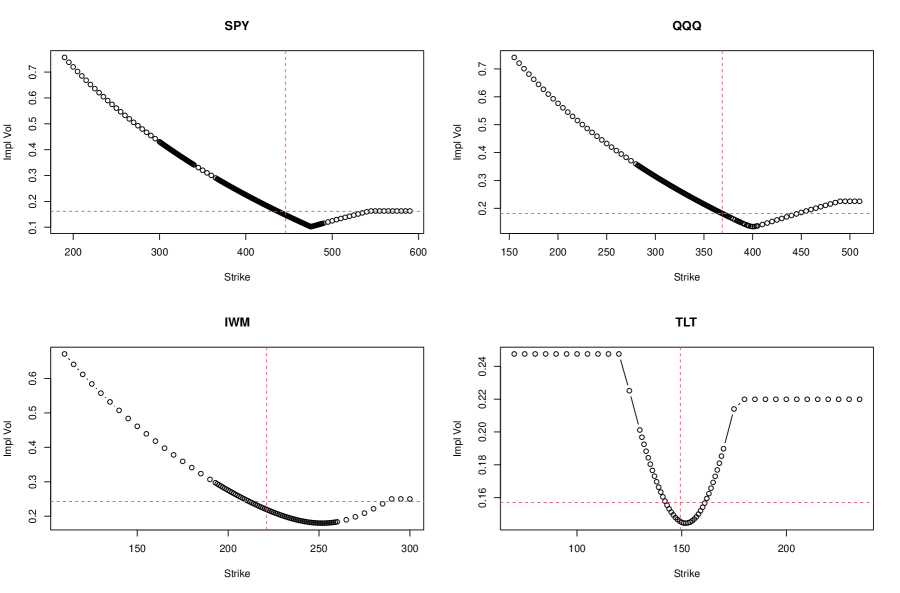
Figure 1: The volatility ‘smiles’ of the the October 15, 2021 option series (calls) as observed and calculated on August 13, 2021 (EOD) for the three market index ETFs, SPY, IWM and QQQ and on August 18, 2021 (EOD) for the TLT ETF.

Figure 1 above displays the calculated implied volatility smile of the October 15, 2021 option series for these three ETFs, SPY, IWM and QQQ, as were quoted on August 13, 2021, each with 63 days to expiration (DTE). Several days later, on August 18, 2021, we obtained the corresponding quote for the TLT, but now with 57 DTE. For each ETF, the EOD option’s market prices (for puts and calls) at the corresponding strikes were recorded along with the BSM-based calculated delta and implied volatility as were provided by the brokerage firm. As reference, we also marked on these plots (in red) the current spot’s (ETF) price $S$ along with the ATM (BS-based) calculated implied volatility (IV) for each ETF. As can be seen from these figures, the options of the three market index ETFs exhibit a highly pronounced skew in their volatility ‘smile’ whereas the option on the TLT ETF do not (likely only reflective of market’s expectations of actions by the Federal Reserve).

However, since typically in the retail world, the calculated option’s implied volatility (as well as other associated quantities, such as the option’s delta) are all calculated based on the Black-Scholes formula in (1), the noted distortion in the volatility smile (or surface) is nonetheless also indicative that the underlying log-normal distribution of the Black-Scholes model (with its distinctive positive skew measure) is a poor choice to serve as RND in such instances involving a stochastic volatility structure as that of Heston’s (1993) (see (25) below); particularly in those instances which admit a negatively skewed RND. To illustrate the extent of the “inaptness” of using the log-normal distribution as RND (the BS formula in (1)) for the option valuation in such skewed cases, we have calibrated for each of these four ETFs the appropriate Heston’s SV model to fit the observed market option data (i.e. on the October 15, 2021 option series for each) and derived from it the underlying RND of the Heston’s model (HS). This RND which is obtained both theoretically, using (26) and (3), and via Monte-Carlo simulations of (25), will serve us as a benchmark for comparison.

For each option series, the available market data consists of the $N$ strikes, $K_{1},\dots,K_{N}$ with corresponding call option (market) prices $C_{1},\dots,C_{N}$. As standard measure of the goodness-of-fit between the model-calculated option prices $C^{\tiny{Model}}(K_{i}),\ i=1,\dots,N$ and the given option market price $C_{i},\ i=1,\dots,N$, we used the Mean Squared Error, MSE,

$$MSE(Model)=\frac{1}{N}\sum_{i=1}^{N}(C^{{{Model}}}(K_{i})-C_{i})^{2}.$$

Clearly, it is expected that within the scope of the SV model described in (25), the well-calibrated Heston’s model will results with a smaller Mean Squared Error as compared to the Black-Scholes model, so that $MSE(HS)\leq MSE(BS)$. However, as we will see below for the available ETF data, pricing the options by a well-calibrated Generalized Gamma (GG) model (18) also resulted with a smaller MSE. In fact, in all four cases, $MSE(GG)\leq MSE(BS)$. To demonstrate this, we have taken for each ETFs the following steps, (conditional of course on the current spot’s price $S$ and volatility $V_{0}$),

• Model Calibration,

  • For a given model’s parameter, $\vartheta=(\kappa,\theta,\eta,\rho)$ in (40), we use the callHestoncf function of the NMOF package of R to calculate the Heston’s model option prices $C_{i}^{\small HS}$ for each $K_{i}$.

  • To calibrate the Heston SV model, we used the optim($\cdot$) function of R, to minimize $MSE(HS)$ over the model’s parameter, $\vartheta=(\kappa,\theta,\eta,\rho)$.

  • For a given $(\alpha,\nu)$ with $\nu=\sigma\sqrt{t}$, we use (18) to calculate the Generalized Gamma model option prices $C_{i}^{\small GG}$ for each $K_{i}$.

  • To calibrate the GG model, we used the optim($\cdot$) function of R, to minimize $MSE(GG)$ over the model’s parameters, $(\alpha,\nu)$.

  • For a given $\nu$ (where $\nu=\sigma\sqrt{t}$), we use (1)-(2) to calculate the Black-Scholes model option prices $C_{i}^{\small BS}$ for each $K_{i}$.

  • To calibrate the BS model, we used the optimize($\cdot$) function of R, to minimize $MSE(BS)$ over the single model’s parameter $\nu$, (namely $\sigma$).

• Validation

  • Using the calibrated Heston’s parameters, $\hat{\vartheta}$ we drew, utilizing a discretized version of Heston’s stochastic volatility process (25), a large number ($M=30,000$) of Monte-Carlo simulation, observations on $(S_{T},V_{T})$ to obtain the simulated rendition of the Heston’s RND of $S_{t}$, (conditional on $S$ and $V_{0}$, with $t=T-\tau$).

  • Using the calibrated Heston’s parameters, $\hat{\vartheta}$ in (27) we obtain the calculated rendition of the Heston’s theoretical RND of $S_{t}$, (conditional on $S$ and $V_{0}$, with $t=T-\tau$), directly from the characteristics function of $P_{2}$ (see Appendix).

  • Compare all three calibrated risk-neutral distributions of the standardized spot’s price (the rescaled spot priced, $S^{*}_{t}=S_{t}/\mu$, where $\mu=Se^{rt}$) as obtained under the Black-Scholes (BS), Generalized Gamma (GG) and Heston’s (1993) option pricing models (HS).

3.2 Calculating the implied RND under the volatility skew

As we mentioned earlier, the data on the October 15, 2021 option series of the SPY, IWM and QQQ were retrieved as of the closing of trading on Friday August 13, 2021 with 63 days to expiration, so that $t=63/365$ and the prevailing (risk-free) interest rate is $r=0.0016$. This will be common values for this three highly liquid ETFs. The October 15, 2021 option series of theTLT was retrieved on August 18, 2021 with 57 days to expiration, so that $t=57/365$ for that ETF. However, we begin our exposition with the details of the largest (volume-wise) of them, namely the SPY. The cases of the IWM, QQQ and TLT will be treated similarly below.

On that day, the closing price of the SPY was $S=445.92$ and the dividend it pays is at a rate of $\ell=0.0123$. We incorporate the dividend in our calculations along the lines of Remark 1 in Boukai (2021). The reported (BS-based) implied volatility was $IV=16.15\%$ which we will used as our initial value for $V_{0}$ and for $\sigma$. This option series has $N=211$ pairs of strike-price $(K_{i},\ C_{i})$ which were all used to calibrate the Heston’s SV model over the the model’s parameter , $\vartheta=(\kappa,\theta,\eta,\rho)$ with the initial values of $(15,(0.1)^{2},0.1,-0.65)$ and with $V_{0}=IV^{2}=(0.1615)^{2}$. The results of the calibrated values are

$$\hat{\vartheta}=(15.03132587,\ 0.02793781,\ 2,\ -0.77469470).$$

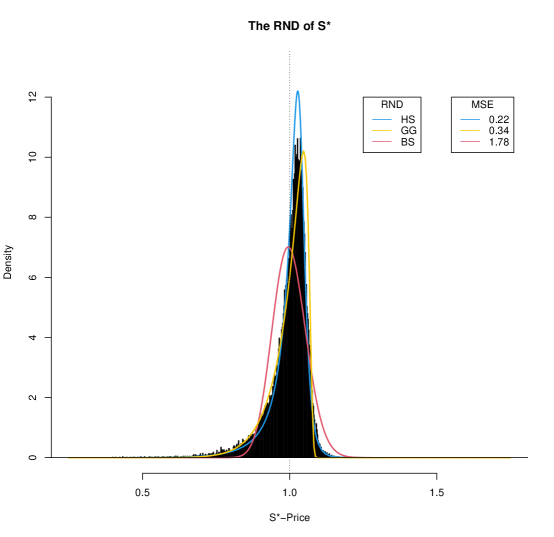
Figure 2: The SPY case- the calculated HS, GG and BS implied RNDs along with the Monte-Carlo distribution of the Spot’s price $S^{*}$, and the corresponding values of the MSE’s

This calibrated parameter, $\hat{\vartheta}$, was then used to calculate, using Heston’s characteristic function in (i.e. (26)), the option prices according to Heston’s SV model (3). This resulted with $MSE(HS)=0.2226429$. The calibrated (least squares estimate) value of $\sigma$ that minimizes $MSE(BS)$ is $\hat{\sigma}=0.137348$, so that $\hat{\nu}_{\tiny BS}=0.137348\sqrt{t}=0.0570619$ to be used for the calculation of the $pdf$ of the ${\cal N}(-\nu^{2}/2,\,\nu^{2})$ distribution which leads to the BS formula in (1) (see Example 3.1 in Boukai (2021) for more details). Next, we calibrated the General Gamma distribution according to the pricing model in (18), with initial values of $\alpha=0.5$ and $\sigma=0.1615$ which resulted with calibrated value of $\hat{\alpha}=0.1554312$ and $\hat{\sigma}=0.1483843$ and an $MSE(GG)=0.339441$ (see Table 3 below). Clearly, in this case of the SPY, the MSE of the GG pricing model is substantially smaller than the MSE of the Black-Scholes model and is similar to that of the Heston’s SV pricing model. Indeed, the MSE of the BS model is over 500% as large as those of the GG and the HS models.

To compare the actual distributions, as calculated under each of these three pricing models, we present in Figure 2 the RNDs of the three implied distributions, calculated base on their respective calibrated parameter values. As an added validation, we plotted these three density curves against the histogram of the Monte-Carlo simulation of the standardized SPY prices using a discretized version of the pricing model in (25) (using the calibrated Heston’s parameters with a seed=452361). This figure clearly demonstrates the ‘inaptness’ of the standard BS formula (1) and hence the log-normal distribution, for modeling option prices in cases which involve negatively skewed price distributions. In fact, the calculated values of the Kurtosis and Skewness measures of each these distributions (see Table 1) is also indicative of the noted lack-of-fit of the BS model in these cases and the apparent close agreement of the GG distribution to the exact risk-neutral distribution of the Heston’s model and that of the simulated price data.

Table 1: Calculated (excess) Kurtosis and Skewness measures for the three distributions depicted in Figure 1 for the SPY option data.

	Measure	HS	GG	BS
	Kurtosis	7.302674	3.536461	0.05234164
	Skewness	-2.050771	-1.580122	0.1715114

Also of interest is the impact of this model’s misspecification on the calculated delta values associated with the option series. It is a standard practice of the retail brokerage houses to provide, along with the market prices for the option chain, also the BS-base calculated delta for each strike (using some ATM implied volatility value). For example, for the ATM strike of $K=445$ the quoted delta is $\Delta^{*}=0.497$ with quoted $IV$ of $0.1489$ whereas under the BS model we calibrated here with $\hat{\sigma}=0.137348$, we obtained $\Delta_{\small{BS}}=0.506$. However, accounting for stochastic volatility in the pricing model, we calculate for this same strike, $K=445$, $\Delta_{\small{HS}}=0.663$ by the (better fitting) Heston SV model, and $\Delta_{\small{GG}}=0.638$, by its close proxy, the GG model. Thus in this case, the BS modeling at the ATM strikes will result with grossly understated delta values (of nearly 25.0%). Without doubt, the impact of this model’s misspecification would have profound hedging implications for the retail trader. To fully appreciate ithe extent of this impact, we present in Figure 3, the values of the Delta function (8) as was calculated for the HS model (using $P1$ and (25)), for the GG model (using (16)) and for the BS model (using $\Phi(d_{1})$ from (1)), along with quoted delta values for the SPY chain.

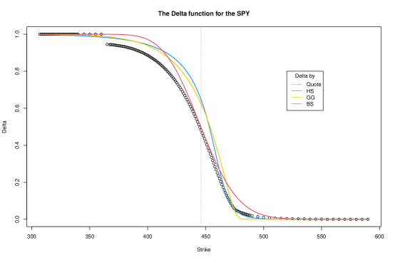
Figure 3: The SPY case- the calculated delta functions under each of the pricing models, HS, GG and BS, along with the quoted delta per each strike $K$ in the October 15, 2021 option series.

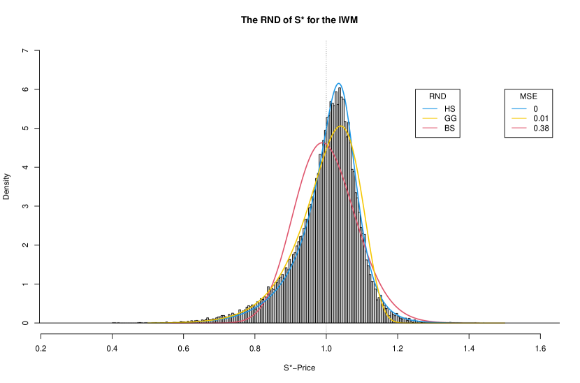
(a) Implied RNDs

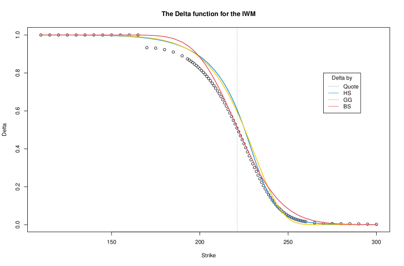
(b) Delta function

Figure 4: The IWM case- (a) the HS, GG and BS implied RNDs along with the Monte-Carlo distribution of the Spot’s price $S^{*}$, and (b) the corresponding delta functions along with the quoted delta per each strike $K$ in the option series.

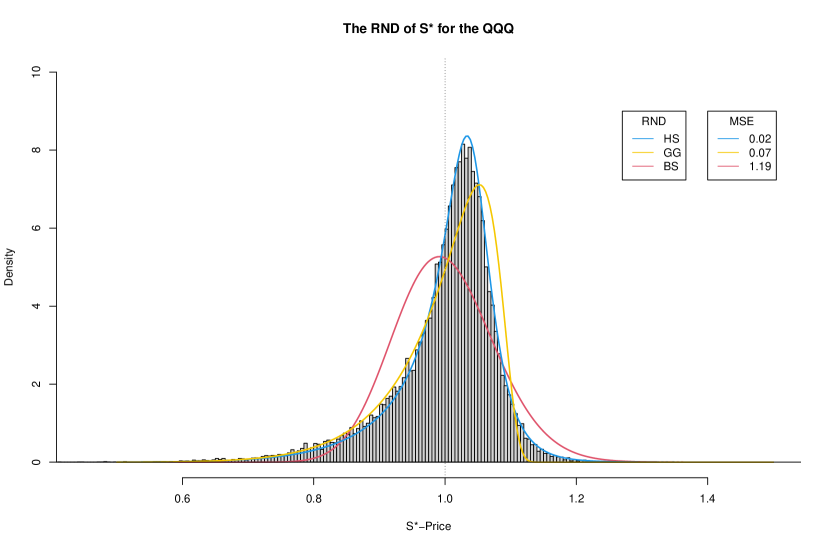
(a) Implied RNDs

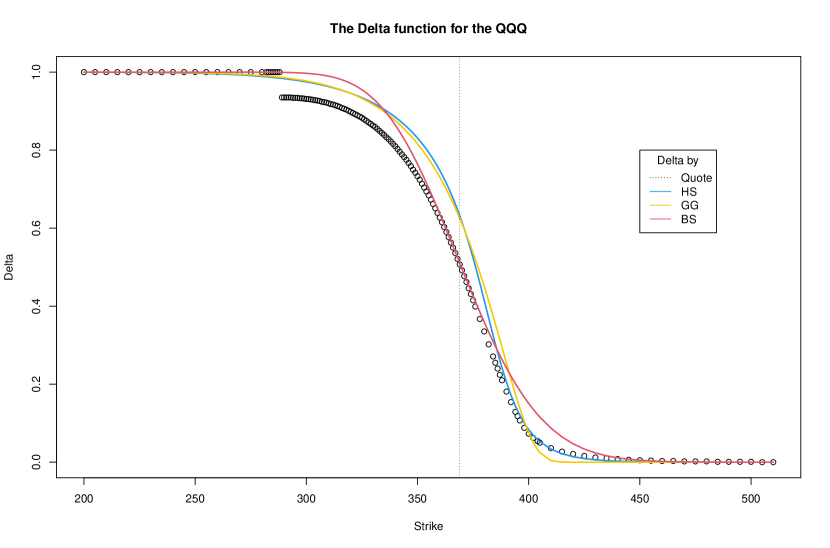
(b) Delta functions

Figure 5: The QQQ case- (a) the HS, GG and BS implied RNDs along with the Monte-Carlo distribution of the Spot’s price $S^{*}$, and (b) the corresponding delta functions along with the quoted delta per each strike $K$ in the option series.

Needless to say, the noted understatement of the quoted (BS -based) delta values as compared to those derived from the SV model also impact the trading strategies. For example, a trader that would sell a 25-Delta strangle based on the quoted values, will sell the $k_{1}=424$ put for $5.215 and the $k_{2}=460$ call for $2.685, collecting a total of $7.90 for it, which amount to 21.9% of the spread between the strikes (for a discussion of this ratio, see Boukai (2020)). On the other hand, if the trader would have priced the 25-Delta strangle according to the GG model (which accounts for the skew), she will sell the $k_{1}=435$ put for $7.205 and the $k_{2}=466$ call for $1.435, collecting a total of $8.64 for it, which amount to 27.9% of the spread between the strikes. Clearly collecting a higher premium for the same 25-delta strangle.

The situation with the other two market-index ETF’s, IWM and QQQ, is very similar to the one describing the SPY–see the corresponding depiction of their volatility ‘smiles’ in Figure 1. Following a similar calibration and validation approach, we present (implied) the price distributions derived from the IWM option data Figure 4 (a) and the QQQ option data Figure 5 (a). The calculated values of the corresponding delta functions are displayed in Figure 4 (b) and Figure 5 (b). Further, to serve as contrasting illustration, we present in Figure 6 the three implied price distributions derived from the TLT ETF option series, along with the corresponding calculated delta functions for that ETF. The situation with the TLT ETF is clearly different, as compared to the three market-index ETFs (SPY, IWM and QQQ) which exhibit pronounced skew of their volatility ‘smile’. In the case of the TLT) ETF, with a relatively intact volatility ‘smile’ (see Figure 1) the implied RNDs are relatively symmetric and three option pricing models (HS, GG and BS) yield very similar results. In Table 2 we provide a summary of the goodness-of-fit of each of the pricing models as measured by the respective MSE for each of the four ETFs. A corresponding comparison of the ATM delta calculations under each of the option price models is presented in Table 3. In Table 3 we provide a summary of the goodness-of-fit as measured by the respective MSE for each of the ETFs. Some of the technical details are provided in Section 4.1 below.

Table 2: The goodness-of-fit as measured the respective MSE for each of the four ETFs .

	ETF	HS	GG	BS
	SPY	0.2226429	0.339441	1.781981
	IWM	0.001900968	0.01419628	0.3750478
	QQQ	0.02418013	0.06561134	1.193867
	TLT	0.03423748	0.04618725	0.04341321

Table 3: Comparison of the the quoted ATM delta $\Delta^{*}$ of the four market ETF to those calculated under each of the three option pricing models.

	ETF	$S$	ATM $K$	$\Delta^{*}$	$\Delta_{\small{BS}}$	$\Delta_{\small{GG}}$	$\Delta_{\small{HS}}$
	SPY	445.92	445	0.497	0.506	0.638	0.663
	IWM	221.13	221	0.510	0.516	0.598	0.610
	QQQ	368.82	369	0.507	0.503	0.625	0.632
	TLT	149.35	150	0.511	0.453	0.477	0.467

4 Summary and discussion

As was illustrated in all the above examples, the Heston (1993) option pricing model (as in (25) and (3)) which accounts for the presences of stochastic volatility, produces as expected, the best results overall as compared to the Black-Scholes option pricing model (1) with its presumed constant volatility. If available, a well-calibrated Heston’s model, will always result in a better fit to realistic market option data (indeed, resulting with $MSE(HS)<MSE(BS)$) and would be the default modeling choice for the practitioner. Unfortunately however, the complex calculations and calibration process of the Heston’s option pricing model (see Appendix) renders it inaccessible to many of the retail option traders. In comparison, the calculations and calibration of the option pricing model under the Generalized Gamma distribution as RND are substantially simpler and straightforward (and could potentially be accomplished within and Excel spreadsheet). As was demonstrated earlier, the GG model is significantly more accurate than the Black-Scholes model for the pricing of the options in a skewed stochastic volatility environments as those exhibited (a͡t present times) by the three markets ETFs, SPY, IWM and QQQ. In fact, in situations which imply negatively skewed price-distributions as RND, the Black-Scholes pricing model, and hence the log-normal distribution as RND, will surely be inferior to the Generalized Gamma distribution, and surely to Heston’s SV pricing model in fitting realistic option market data. In such situations one would realize $MSE(GG)<MSE(BS)$ and would want to adopt the GG distribution as RND for the underlying pricing model. In contrast, in situations such as the one exhibited by the TLT ETF, one would realize $MSE(GG)\approx MSE(BS)$, as all three option pricing models (including Heston’s) produce similar results. Although not expressly covered by the examples we analyzed here, we have grounds to believe that the same conclusion could be arrived upon using the Inverse Generalized Gamma (see Section 2.2) as an RND in situations involving positively skewed (implied) RND in the option pricing model. In all, both of these versions of the Generalized Gamma distribution could serve as useful proxies to the exact Heston’s RND and hence produce superior results to those obtained by the Black-Scholes model in an environment involving stochastic volatility. Thus given the market option data, one could simply calculate $MSE(BS),MSE(GG)$ (and if needed also $MSE(IGG)$) and adopt the option pricing model which produces the better fit.

4.1 Some technical notes

• The the October 15, 2021 option series data files SPY_63.csv, IWM_63.csv, and QQQ_63.csv as were obtained on the EOD of August 13, 2021 and that of TLT_57.csv obtained at the EOD of August 18, 2021, are available from the author upon request. Their basic summary information is provided in Table 4 below.

  Table 4: Summary information of the four ETFs .

  	ETF	$S$	DTE	N	Quoted IV	Div. Rate
  	SPY	445.92	63	211	16.15%	1.23%
  	IWM	221.13	63	93	24.30%	0.63%
  	QQQ	368.82	63	160	18.13%	0.43%
  	TLT	149.35	57	66	15.71%	1.46%

• The R function dgamma and pgamma were used to calculate the $pdf$ and $cdf$ in (10) and hence in the calculation of (18).

• The cfHeston and callHestoncf functions of the NMOF package of R, were used in the calculation of (26) and (3).

• A modification of the callHestoncf function of the NMOF package of R was used to calculate (27).

• The optim and optimize functions of R were used in the calibration of the three models (HS, GG and BS) for the available option data.

• The initial and the calibrated values of $\vartheta=(\kappa,\theta,\eta,\rho)$ of the Heston’s model were:

  • $(15,(0.1)^{2},0.1,-0.65)$ and  $(15.03132587,\ 0.02793781,\ 2,\ -0.77469470)$.

  • $(5,(0.1)^{2},0.6,0)$ and   $(4.97834286,0.04032166,1.09837930,-0.59905916)$.

  • $(3.5,(0.2)^{2},0.5,-0.5)$   and  $(3.47635183,0.06382197,1.13505528,-0.69137767)$.

  • $(3,(0.1)^{2},0.1,0.1)$   and  $(2.99997881,0.01459405,0.10011507,0.10007980)$.

• For the Monte-Carlo simulation of (25) we employed the (reflective version of) Milstein’s (1975) discretization scheme (see also Gatheral (2006)) with seeds =4569 (QQQ), =777999 (IWM) and =452361 (SPY) and = 121290 (TLT).

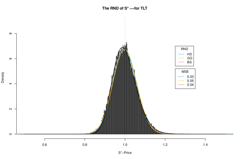
(a) Implied RNDs

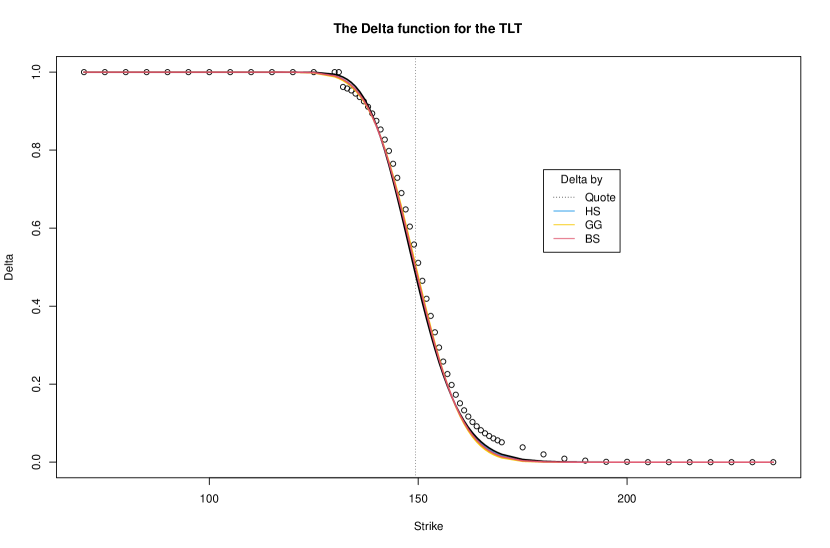
(b) Delta function

Figure 6: The TLT case- (a) the HS, GG and BS implied RNDs along with the Monte-Carlo distribution of the Spot’s price $S^{*}$, and (b) the corresponding delta functions along with the quoted delta per each strike $K$ in the option series.

5 Appendix

Heston (1993) considered the stochastic volatility model describing the price-volatility dynamics (of ${\cal{S}}=\{S_{t},\,t\geq 0\}$ and ${\cal{V}}=\{V_{t},\,t\geq 0\}$) as described via a system of stochastic deferential equations given by,

$$dS_{t}= rS_{t}dt+\sqrt{V_{t}}S_{t}dW_{1,t}$$ (25)

$$dV_{t}= \kappa(\theta-V_{t})+\eta\sqrt{V_{t}}dW_{2,t},$$

where $r$ is the risk-free interest rate, $\kappa,\ \theta$ and $\eta$ are some constants (as discussed in Section 1) and where $W_{1}=\{W_{1,t},\,t\geq 0\}$ and $W_{2}=\{W_{2,t},\,t\geq 0\}$ are two Brownian motion processes under (under the risk neutral probability $\mathbb{Q}$) with $d(W_{1}W_{2})=\rho dt$ for some $\rho^{2}\in(0,1)$. Heston (1993) offered $C_{S}(K)$ in (3) as the solution to the option valuation under the above SDE and provided (semi) closed form expressions to the probabilities $P_{1}$ and $P_{2}$ that comprise it.

These closed form expressions are given for $j=1,2$ by,

$$P_{j}=\frac{1}{2}+\frac{1}{\pi}\int_{0}^{\infty}{\cal R}\text{e}\left[\frac{e^{-i\omega k}\psi_{j}(\omega,t,v,x)}{i\omega}\right]d\omega,$$ (26)

where with $x:=\log{(S)}$, $k:=\log{(K)}$, $b_{1}=\kappa-\rho\eta,\ \ b_{2}=\kappa$ and $\psi_{j}(\cdot)$ is the characteristics function

$$\psi_{j}(\omega,t,v,x):=\int_{-\infty}^{\infty}e^{i\omega s}p_{j}(s)ds\equiv e^{B_{j}(\omega,t)+D_{j}(\omega,t)v+i\omega x+i\omega\,rt}.$$

Here $p_{j}(\cdot)$ is the $pdf$ of $s_{T}=\log(S_{T})$ corresponding to the probability $P_{j},\ j=1,2$ and

$$B_{j}(\omega,t)=\frac{\kappa\theta}{\eta^{2}}\{(b_{j}+d_{j}-i\omega\rho\eta)t-2\log(\frac{1-g_{j}e^{d_{j}t}}{1-g_{j}})\}$$

$$D_{j}(\omega,t)=\frac{b_{j}+d_{j}-i\omega\rho\eta}{\eta^{2}}(\frac{1-e^{d_{j}t}}{1-g_{j}e^{d_{j}t}})$$

$$g_{j}=\frac{b_{j}-i\omega\,\rho\eta+d_{j}}{b_{j}-i\omega\rho\eta-d_{j}}$$

$$d_{j}=\sqrt{(i\omega\rho\eta-b_{j})^{2}-\eta^{2}(2i\omega u_{j}-\omega^{2})}.$$

Note that by a standard application of the Fourier transform obtains (see for example Schmelzle (2010)) that the $pdf$ $p_{j}(\cdot)$ of $s_{T}=\log(S_{T})$, can be computed, for any $s\in{\mathbb{R}}$, as

$$p_{j}(s)=\frac{1}{\pi}\int_{0}^{\infty}{\cal R}\text{e}\left[{e^{-i\omega s}\psi_{j}(\omega,t,v,x)}\right]d\omega.$$ (27)

Regardless of their complexities, efficient numerical routines such as the cfHeston and callHestoncf functions of the NMOF package of R, are readily available nowadays to accurately compute the values of $\psi_{j}$ and hence of $P_{j}$ and the call option values $C_{S}(K)$ in (3), for given $t,s$ and $v$ and any choice of $\vartheta=(\kappa,\theta,\eta,\rho)$.

References

- [1] Albrecher, H., Mayer, P., Schoutens, W. and Tistaer, J., (2007). The Little Heston Trap. The Wilmott Magazine, 83–92.
- [2] Alfonsi A., (2010) High order discretization schemes for the CIR process: Application to affine term structure and Heston models. Math. Comp. 79(269), 209–237.
- [3] Andersen L., (2008) Simple and efficient simulation of the Heston stochastic volatility model. J. Comput. Finance, 11(3), 2008, 1–42.
- [4] Black F., and Scholes M., (1973). The pricing of options and corporate liabilities. The Journal of Political Economy, 637-654.
- [5] Bakshi G., Cao C. and Chen Z., (1997) . Empirical Performance of Alternative Option Pricing Models. The Journal of Finance, Vol. LII, No. 5, 2003-2049.
- [6] Boukai B. (2020). How Much is your Strangle Worth? On the Relative Value of the delta-Symmetric Strangle under the Black-Scholes Model Applied Economics and Finance, Vol. 7, No. 4; July 2020 https://doi.org/10.11114/aef.v7i4.4887
- [7] Boukai B. (2021). On the RND under Heston’s Stochastic Volatility Model. Available at SSRNhttps://ssrn.com/abstract=3763494
- [8] Cox J.C. and Ross S., (1976) The valuation of options for alternative stochastic processes. J. Fin. Econ. 3:145-66.
- [9] Feller W., (1951) Two singular diffusion problems. Ann. Math. 54(1), 173–182.
- [10] Figlewski S., (2010). “Estimating the Implied Risk Neutral Density for the U.S. Market Portfolio”, in Volatility and Time Series Econometrics: Essays in Honor of Robert F. Engle, (eds. Tim Bollerslev, Jeffrey Russell and Mark Watson) Oxford University Press, Oxford, U.K.
- [11] Figlewski S., (2018). Risk Neutral Densities: A Review. Available at SSRNhttp://ssrn.com/abstract=3120028.
- [12] Gatheral, J., (2006). The Volatility Surface, John Wiley and Sons, NJ.
- [13] Grith M. and Krätschmer V., (2012) “Parametric Estimation of Risk Neutral Density Functions”, in: Ed: Duan JC., Härdle W., Gentle J. (eds) Handbook of Computational Finance Springer Handbooks of Computational Statistics. Springer, Berlin, Heidelberg.
- [14] Heston S.L., (1993) A closed-form solution for options with stochastic volatility with applications to bond and currency options. Rev. Financ. Stud. 6(2), 327–343.
- [15] Jackwerth, J. C., (2004). Option-Implied Risk-Neutral Distributions and Risk Aversion Research Foundation of AIMR, Charlotteville, NC
- [16] Jackwerth, J. C. and Rubinstein, M., (1996). Recovering Probability Distributions from Option Prices. The Journal of Finance, 51, no. 5: 1611-631.
- [17] Jiang, L. (2005). Mathematical Modeling and Methods of Option Pricing, Translated from Chinese by Li. C, World Scientific, Singapore.
- [18] Kiche J., Ngesa O. and Orwa, G. (2019) On Generalized Gamma Distribution and Its Application to Survival Data International Journal of Statistics and Probability; Vol. 8, No. 5, :https://doi.org/10.5539/ijsp.v8n5p85
- [19] Lemaire, V., Montes, T. and Pagès, G., (2020). Stationary Heston model: Calibration and Pricing of exotics using Product Recursive Quantization. Available at arXiv [q-fin.MF]: arXiv:2001.03101v2.
- [20] Merton, R., (1973). Theory of rational option pricing. The Bell Journal of Economics and Management Science, 141-183.
- [21] Mil’shtein, G. N. (1975). Approximate Integration of Stochastic Differential Equations. Theory of Probability & Its Applications, 19 (3), 557–562.
- [22] Mizrach, B. (2010). “Estimating Implied Probabilities from Option Prices and the Underlying” in Handbook of Quantitative Finance and Risk Management (C.-F. Lee A. Lee and J. Lee (eds.)). Springer Science Business Media.
- [23] Mrázek, M. and Pospíšil, J. (2017). Calibration and simulation of Heston model. Open Mathematics— Vol. 15(1), https://doi.org/10.1515/math-2017-0058.
- [24] R Core Team, (2017). R: A Language and Environment for Statistical Computing. Vienna, Austria, https://www.R-project.org/
- [25] Stacy, EW. (1962). A generalization of the gamma distribution. The Annals of Mathematical Statistics, 33, 1187-1192.
- [26] Stein J. and Stein E., (1991). Stock price distributions with stochastic volatility: An analytic approach. Rev. Financ. Stud. 4(4), 727–752.
- [27] Schmelzle, M., (2010). Option Pricing Formulae using Fourier Transform: Theory and Application. Technical Report, Available on line at https://pfadintegral.com/articles/option-pricing-formulae-using-fourier-transform/
- [28] Savickas, R., (2002). A simple option formula. The Financial Review, Vol 37, 207-226.
- [29] Savickas, R., (2005). Evidence on delta hedging and implied volatilities for the Black-Scholes, gamma, and Weibull option pricing models. The Journal of Financial Research, Vol 18:2, 299-317.
- [30] Thurai, M. and Bringi, V. N. (2018) Application of the Generalized Gamma Model to Represent the Full Rain Drop Size Distribution Spectra. Journal of Applied Meteorology and Climatology, Vol. 57, No. 5, 1197-1210.
- [31] Wiggins, B. J., (1987). Option values under stochastic volatility: Theory and empirical estimates. Journal of Financial Economics, Vol. 19(2), 351-372