Framework for liquid crystal based particle models

Abstract

Long-range e.g. Coulomb-like interactions for (quantized) topological charges in liquid crystals are observed experimentally, bringing open question this article is exploring: how far can we take this similarity with particle physics? Uniaxial nematic liquid crystal of ellipsoid-like molecules can be represented using director field $\vec{n}(x)$ of unitary vectors. It has topological charge quantization: integrating field curvature over a closed surface $\mathcal{S}$, we get 3D winding number of $\mathcal{S}\to S^{2}$, which has to be integer - getting Gauss law with built-in missing charge quantization if interpreting field curvature as electric field. This article proposes a general skyrmion-like mathematical framework to extend this similarity with particle physics to biaxial nematic: additionally recognising intrinsic twist of uniaxial nematic, having 3 distinguishable axes - e.g. allowing to construct hedgehog configuration with one of 3 axes: with the same topological charge, but different energy/mass - getting similarity with 3 leptons. The proposed approach has vacuum dynamics as: electromagnetism from 3D rotation dynamics + Klein-Gordon-like equation for twist corresponding to quantum phase. If extending to 4D field with 4 distinguishable axes, e.g. with time axis rotations replaced by boosts , we also get second set of Maxwell equations for GEM (gravitoelectromagnetism) approximation of general relativity.

Keywords: field theory, topological solitons, liquid crystals, Landau-de Gennes model, skyrmions, long-range interaction, electromagnetism, gravitomagnetism, particle physics

I Introduction

While quantum field theories are often imagined as Feynman ensemble of classical fields, the latter still contain crucial issues - maybe worth resolving before the 2nd quantization, like:

1. missing charge quantization: Gauss law should only return integer multiplicities of $e$ (+confined fractional),

2. missing regularization: infinite energy of electric field of charge, bounded by 511keV released in annihilation.

In liquid crystals there are experimentally realized quantized topological charges with long-range interactions, e.g. resembling quadrupole-quadrupole [1], dipole-dipole [2], Coulomb [3] or even stronger [4] interactions - suggesting resolution to both problems on classical field level, for example using Faber’s approach ([5, 6, 7, 8, 9]) this article extends on - summarized in Figure 1 (gathered materials):

1. Interpret curvature of e.g. field vector $\vec{n}$ as electric field, making Gauss law counts its topological charge,

2. Use Higgs-like potential e.g. $V=(\|\vec{n}\|^{2}-1)^{2}$, allowing for e.g. $\vec{n}\to 0$ regularization of singularities.

Such reparation before 2nd quantization could also improve our understanding of quantum field theories - of (e.g. EM) field configurations represented in Feynman diagrams, starting with: what is mean energy density in given distance from electron?

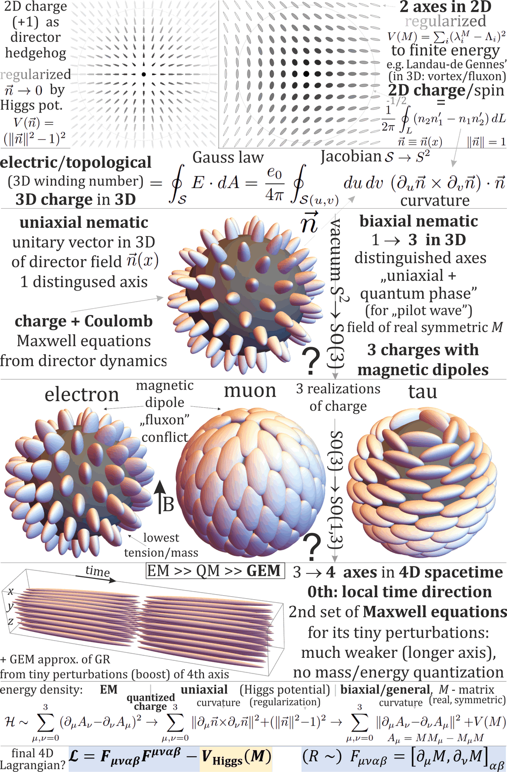
Figure 1: Unitary vector $\vec{n}\equiv\vec{n}(x)$ ”director” field has quantization of topological charge, for which in liquid crystals experiments there were obtained long-range interactions - interpreting curvature as electric field, we can get Maxwell equations for their dynamics. Living in 3D suggests to extend it to 3 distinguishable axes representing rotating object - realized e.g. in biaxial nematic, getting 3 types of hedgehog with the same charge, but different energy (like 3 leptons), also magnetic singularity due to the hairy ball theorem. We model such ellipsoid field like stress-energy tensor: with field of real symmetric matrices $M(x)\equiv M=ODO^{T}$ (orthogonal $OO^{T}=I$, $D=\textrm{diag}(\lambda_{1},\lambda_{2},\lambda_{3})$), which prefers some shape as set of eigenvalues due to Higgs-like potential e.g. $V(M)=\sum_{i}(\lambda_{i}-\Lambda_{i})^{2}$ for some fixed model parameters: $\Lambda_{1}>\Lambda_{2}>\Lambda_{3}$ - allowing to regularize singularity (discontinuity in the center) to finite energy as in top diagrams. Reminding that we live in 4D spacetime suggests to add 0th time axis as the longest ($D=\textrm{diag}(\lambda_{0},\lambda_{1},\lambda_{2},\lambda_{3})$) - having the strongest tendency to be aligned in parallel, acting as local time direction. Mass/energy should enforce tiny perturbations as curvature of this time axis, with dynamics given by second set of Maxwell equations for GEM approximation of the general relativity. Lorentz invariance suggests SO(3) should become SO(1,3) including boosts.

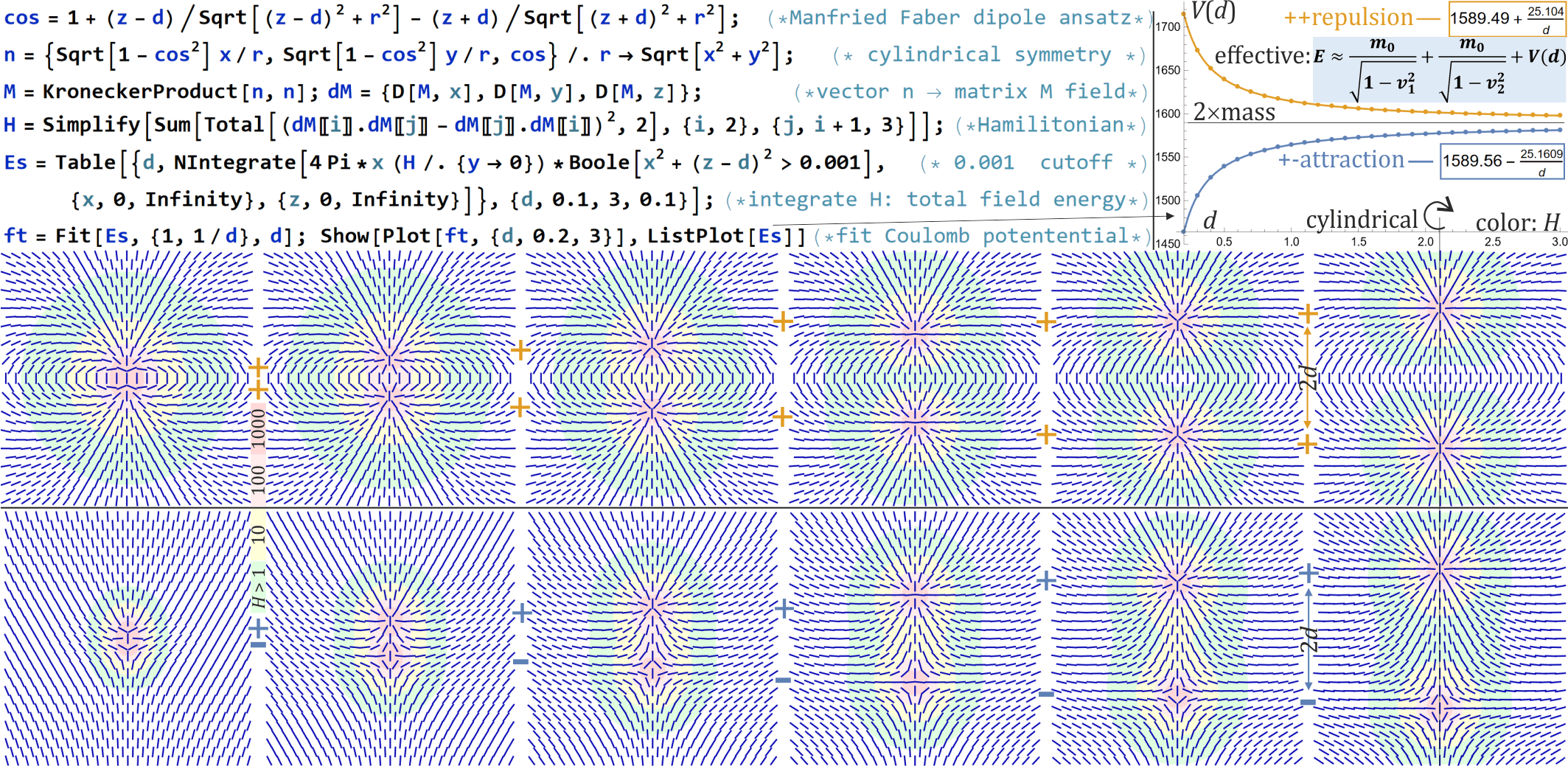
Figure 2: Calculation of Coulomb effective potential with shown Mathematica source (extended in GitHub). For ”+-” or ”++” pair of topological charges, there was postulated ansatz [6]: cylindrically symmetric configuration of unitary vector field $n$ in agreement with electric field of two elementary charges (in GitHub verified satisfaction of variation equation). Such various distance configurations are shown with visualized $H$ density. Seen as uniaxial nematic it corresponds to $M=nn^{T}$ matrix field, as discussed here with static energy density $H=\sum_{1\leq i<j\leq 3}\|[\partial_{i}M,\partial_{j}M]\|^{2}$. Integrating this energy density with cutoff around two singularities, there was numerically obtained $E(d)\approx 1590\pm 25/d$ distance-energy dependence as in Coulomb law (shown values and fit). Finally the two singularities are to be regularized with Higgs-like potential e.g. $(1-\|n\|^{2})^{2}$, due to Lorentz invariance leading to $m_{0}\to m_{0}/\sqrt{1-v^{2}}$ energy scaling. To avoid infinite energy of singularities in charges there was used cutoff above, which finally should be replaced with regularization by Higgs-like potential - as discussed and calculated in [9], leading to deformations of Coulomb interaction in tiny distances in agreement with the running coupling effect.

Liquid crystals use ellipsoid-like molecules, which if cylindrically symmetric (uniaxial nematic) can be represented with director field $\vec{n}\equiv\vec{n}(x)$ of unitary vectors, this way allowing for (quanitzed) topological charges e.g. hedgehog-like configurations. They get long-range e.g. Coulomb-like interaction as in Figure 2: total energy of the field (as integrated energy density: Hamiltonian) for two charges in various distances behaves as in Coulomb potential.

Such 3D topological charge as 3D winding number [10] of $\vec{n}$ restricted to $\mathcal{S}\to S^{2}$, can be calculated by integrating over closed surface $\mathcal{S}$ the Jacobian of this function - which turns out curvature of this field. Therefore, interpreting (e.g. vector) field curvature as electric field, we get Gauss law with built-in charge quantization as topological.

The center of such topological charge naively has field discontinuity, which would mean infinite energy - like of electric field around point charge. To prevent it, we could make a cutoff as in Fig. 2, in liquid crystals we can imagine there is no molecule in the center of e.g. hedgehog. However, for a field there should be value everywhere - we need to regularize it, deform to finite energy, e.g. at most 511 keVs for electron - released in annihilation. There can be used $V(\vec{n})=(\|\vec{n}\|^{2}-1)^{2}$ Higgs potential: preferring unitary vectors, also allowing to deform e.g. to $\vec{n}=0$ in the center of singularity to prevent infinity. Massless dynamics of this vacuum (Goldstone bosons) can be chosen to resemble electromagnetism by interpreting curvature as electric field. Experimental consequence of such regularization to finite energy is deformation of Coulomb interaction in tiny distances, which agrees with known running coupling effect [9]. For regularization of a more general field, we need potential with topologically nontrivial minimum, e.g. $S^{2}$: $\|\vec{n}\|=1$ $S^{2}$ for uniaxal nematic, SO(3) for biaxial nematic, like in Landau-de Gennes model [11].

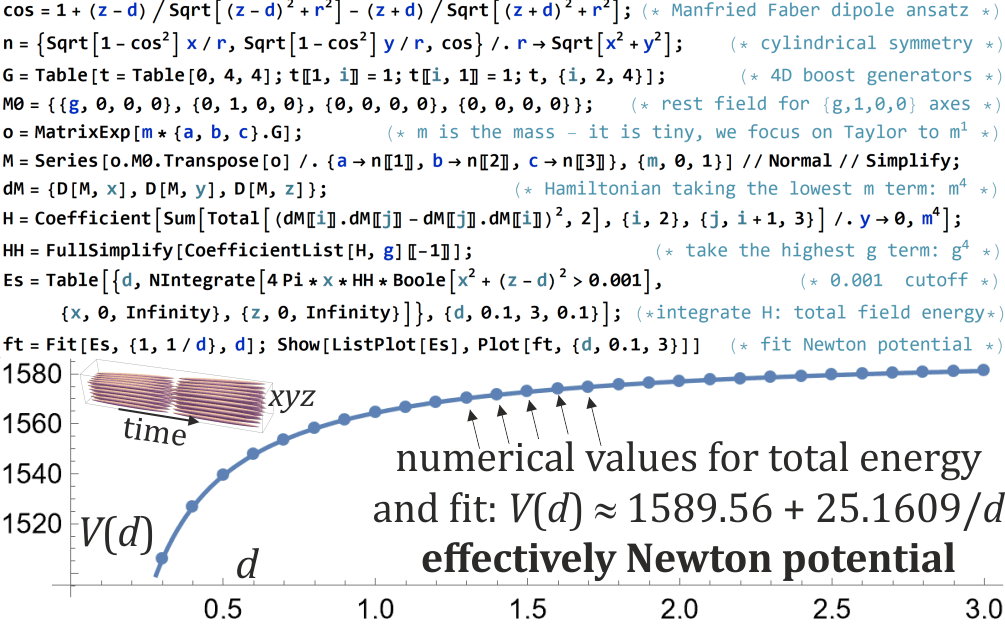
Figure 3: Example of simplified calculation of Newton effective potential (in GitHub) - analogously as in Fig. 2, but this time instead of large spatial rotations, using tiny tilts of 0th time axis for gravity (no mass quantization). Spherically symmetric curvature sources would have increased energy with reduced distance, hence to get attraction there was used dipole ansatz for microscopic scenarios like pair creation, hopefully averaging to spherically symmetric gravity. Final calculations will need further work.

Generic objects in 3D have 3 distinguishable axes, SO(3) rotations - like molecules in experimentally challenging biaxial nematic liquid crystals ([11, 12, 13]). Similarly to Landau-de Gennes model, we will discuss using field of real symmetric matrices $M(x)\equiv M=ODO^{T}$ (orthogonal $OO^{T}=I$, $D=\textrm{diag}(\lambda_{1},\lambda_{2},\lambda_{3})$) for this purpose: which due to potential prefers some fixed set of eigenvalues $\Lambda_{1}>\Lambda_{2}>\Lambda_{3}$, but allows for their $(\lambda_{i})$ deformation/regularization to prevent infinite energy in singularity using e.g. $V(M)=\sum_{i}(\lambda_{i}-\Lambda_{i})^{2}$ Higgs-like potential, as in top-right diagram in Fig. 1. Instead of integer, this 2D configuration has 2D topological charge +1/2 due to symmetry: that ellipsoid rotated by $\pi$ is the same ellipsoid, what also agrees with quantum rotation operator: ”rotating spin $s$ particle by $\phi$ angle, rotates phase by $s\phi$” - suggesting to interpret 2D topological charge as spin, 3D as electric charge. Additionally, fluxons in superconductor are well known 2D topological charges - like spin associated with magnetic field. Also, voricity works analogously to magnetic field e.g. in Aharonov-Bohm ([14, 15]) and Zeeman effect [16].

Distinguishing two types of rotation (of $\Lambda$ shape): twist of biaxial nematic, and two tilts as in Fig. 4, will allow to assign them different energy scales. Going to 4D, we can imagine additional much longer 0th time axis undergoing tiny perturbations - naively rotations of SO(4), but Lorentz invariance suggests to use SO(1,3) with boosts instead. Finally the discussed approach allows to unify 3 types of vacuum dynamics (far from particles/singularises):

• electromagnetism (EM) of relatively high energy - governed by Maxwell (wave-like) equations, corresponding to tilts, already in uniaxial nematics (e.g. Coulomb: [3]),

• quantum phase ($\arg(\psi)$) evolution of much lower energies ($\hbar c$ in QED Lagrangian) - corresponding to twists, governed by Klein-Gordon-like (wave-like) equation,

• gravitoelectromagnetism (GEM) approximation of general relativity - 2nd set of (wave-like) Maxwell equations for tiny perturbations (boosts) of 0th time axis.

Such field of 3 distinguishable axes allows to construct hedgehog-like configuration of one of 3 axes as in Fig. 1 - they have the same 3D topological charge acting as electric charge, but require different regularization/deformation - should have different mass/energy, resembling 3 leptons. Additionally, the hairy ball theorem [17] says that we cannot continuously align such axes on the sphere - requiring additional spin-like singularities resembling fluxons, which should correspond to magnetic dipole moment of leptons. In particle physics three families are common (also for quarks) - the discussed approach suggests it might be a consequence of just living in 3D.

The difference between uniaxial and biaxial nematic can also be imagined as recognizing intrinsic rotation (referred as twist) of elongated molecule - here adding to electromagnetism (referred as tilts) single low energy vacuum degree of freedom, which hopefully well corresponds to quantum phase, pilot wave. Louis de Broglie hypothesised that electron has intrinsic periodic process $\approx 10^{21}$ Hz, also called zitterbewegung as consequence of Dirac equation (use $E=mc^{2}$) - now confirmed experimentally [18], also in Bose-Einstein condensate analogs [19]. Hence the discussed corresponding configurations should enforce such periodic process, like spin precession [20] or rotation (twist) of this additional degree of freedom - leading to ”pilot wave” coupled with such electron. For 3D case there is obtained Klein-Gordon-like equation, but missing gravitational mass - hopefully added in 4D considerations.

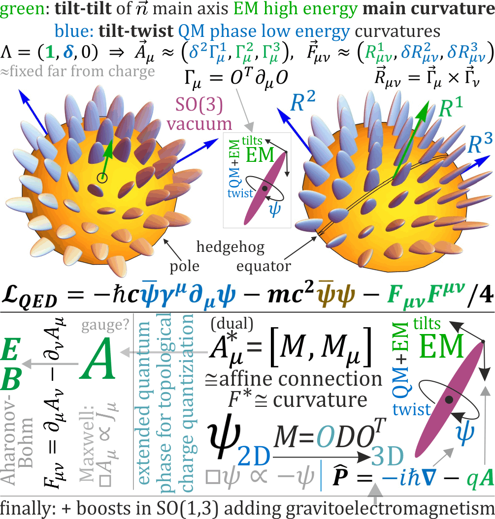
Figure 4: Top: parts of hedgehog of the longest $\vec{n}$ main axis of biaxial-nematic-like field. This axis can tilt in two directions already in uniaxial nematic, in biaxial there are additionally recognized its twists - here tilts correspond to high energy EM dynamics, twists to low energy QM phase dynamics. Such local rotation is affine connection $\Gamma_{\mu}=O^{T}(\partial_{\mu}O)$: antisymmetric matrix we can interpret as local rotation vector $\vec{\Gamma}_{\mu}:=\left((\Gamma_{\mu})_{32},(\Gamma_{\mu})_{13},(\Gamma_{\mu})_{21}\right)$. It corresponds to $A_{\mu}$ four-vector weighted with shape $\lambda\approx\Lambda$ (far from charge fixed by potential e.g. $V=\sum_{i}(\lambda_{i}-\Lambda_{i})^{2}$) distinguishing high energy tilts from low energy twists. Curvatures $\vec{R}_{\mu\nu}=\vec{\Gamma}_{\mu}\times\vec{\Gamma}_{\nu}$ after weighting with shape become dual $F^{*}_{\mu\nu}$ tensor: containing high energy tilt-tilt component $R^{1}_{\mu\nu}$ corresponding to EM, and low energy tilt-twist $R^{2}_{\mu\nu},R^{3}_{\mu\nu}$ corresponding to QM phase like in QED-like Lagrangian. Bottom: due to Aharonov-Bohm-like arguments, there is belief that $A$ four-vector is more fundamental than $E,B$ fields, however, it leaves gauge freedom. It also allows for non-integer charges like half-electron - to prevent that, there is postulated more fundamental field $M$ which (quantized) topological charge is calculated in Gauss law. This deeper field can be seen as extended quantum phase: from low energetic evolution of $S^{1}$ quantum phase (twists), to SO(3) evolution (+tilts) including also electromagnetism with built-in (topological) charge quantization, getting simple EM+QM unification (+GEM with 4D field, SO(1,3) vacuum).

Analogous view on wave-particle duality has also allowed for experimental realizations of hydrodynamical analogs of many quantum phenomena with hydrodynamical wave-particle duality objects: walking droplets. For example double slit interference [21] (corpuscle travels one trajectory, its coupled wave travels all - affecting corpuscle trajectory), unpredictable tunneling [22] (depending on complex history of the field), Landau orbit quantization [23] (coupled wave has to become standing wave for resonance condition in analogy to stationary Schrödinger equation for orbital quantization), Zeeman-like splitting [16] of such quantized orbits (using Coriolis force as analogue of Lorentz force, vorticity as magnetic field ([14])), double quantization [24] (in analogy to $(n,l)$ for atomic orbitals), and recreating quantum statistics with averaged trajectories [25]. There are also known hydrodynamical analogs for Casimir [26] and Aharonov-Bohm effects ([14, 15]). For fluxons as 2D topological charges in superconductor there was experimentally realized e.g. interference [27], tunneling [28] and Aharonov-Bohm [29] effect.

Maximal Entropy Random Walk (MERW) also suggests quantum-like statistics for objects undergoing complex dynamics. Standard diffusion models turn out to only approximate the (Jaynes) maximal entropy principle, necessary for statistical physics models - lacking Anderson-like localization, observed also for neutrons [30]. MERW really does this optimization, getting stationary probability distribution exactly as quantum ground state, with its localization properties ([31, 32, 33, 34]). E.g. for $[0,1]$ range standard diffusion predicts uniform $\rho=1$ stationary probability distribution, while QM and MERW predict localized $\rho\propto\sin^{2}$.

As we live in 4D spacetime, it is tempting to extend from 3 to 4 distinguishable axes by just going from $3\times 3$ to $4\times 4$ real symmetric matrix field $M$ - like the stress-energy tensor, for which $M$ might be microscopic extension. The 0th axis should be the longest - having the strongest tendency to align in nearly parallel way. This way dynamics of its tiny perturbations (rotations or boosts) is governed by additional set of Maxwell equations - with goal to obtain e.g. GEM: confirmed by Gravity Probe B approximation of general relativity. Such tiny perturbation/spatial curvature can be caused e.g. by EM-GEM interaction or activating potential to give particles also gravitational mass. Slowing down of EM propagation through EM-GEM interaction could explain gravitational time dilation and lensing. In contrast to charge corresponding to complete spherical angle, this time we have only tiny curvature - there is no mass quantization.

Like electromagnetism, the discussed approach is viscosity-free, hence experimental realizations would require e.g. superfluid like in famous Volovik ”Universe in a helium droplet” book [35]. Related skyrmion models ([36, 37]) also aim particles - e.g. nuclei resemblance, instead of electric charge using topological charge as baryon number, they lack long-range EM interaction. Also simplified experimental settings could allow to get some interesting correspondence, like vortices going out of biaxial nematic topological charge due to the hairy ball theorem (no spin-less charge). Such models might lead to better understanding of particle physics, providing e.g. suggestion why protons are lighter than neutrons (later Figure 8), hopefully to derive at least parts of the Standard Model as its 2nd quantization.

While the presented general view was already discussed by the author (the first version of [32], [38]), this article finally introduces looking proper basic mathematical framework. The current version is update of work in progress, planned to be extended in the future.

II General quantitative framework

This main section first introduces to obtaining electromagnetism, with built-in charge quantization and regularization, to director field in analogy to Faber approach ([5, 6, 7, 8, 9]). Then there is discussed generalization to biaxial nematic case using field of real symmetric matrices (like stress-energy tensor) preferring shape as $(\Lambda_{i})$ set of eigenvalues.

II-A Gauss law with built-in (topological) charge quantization

Imagine a continuous (director) field of unitary vectors $\vec{n}:\mathbb{R}^{d}\to S^{d-1}$. Restricting it to a closed surface $\mathcal{S}\subset\mathbb{R}^{d}$ gives $\vec{n}:\mathcal{S}\to S^{d-1}$ function, which has some integer number of coverings/windings of this sphere - called topological charge.

This (generalized) winding number, multiplied by sphere area, can be obtained by integrating Jacobian (as determinant of Jacobian matrix) over this closed surface - we would like to interpret this Jacobian e.g. as electric field, making that Gauss law counts this winding number - getting missing built-in charge quantization as topological charge.

In 2D case, analogous e.g. to argument principle in complex analysis, integrating derivative of angle over loop gives $2\pi$ times topological charge ($\vec{n}^{\prime}=d\vec{n}/dL$, $\vec{n}=(n_{1},n_{2})$):

$$\textrm{2D topological charge}=\frac{1}{2\pi}\oint_{L}(n_{2}n^{\prime}_{1}-n_{1}n^{\prime}_{2})\,dL$$

This way we e.g. get quantization of magnetic field in superconductors as fluxon/Abrikosov vortex [39] being 2D topological charge, which also resembles spin as in quantum rotation operator: saying that rotating spin $s$ particle by $\varphi$ angle rotates quantum phase by $s\varphi$. Observe that, as in top of Fig. 1, with liquid crystals we can get spin 1/2 this way as rotating by $\pi$ radians we get the same ellipsoid.

2D topological charges in 3D (vortex, fluxon) seem related with magnetic field lines (also resembling spin), there is experimentally confirmed analogy between magnetic field and vorticity ([14, 15, 16]). In contrast, 3D topological charge in 3D is nearly point-like and in liquid crystals get long-range interactions due to nontrivial vacuum dynamics of director field ([1, 2, 3, 4]). We would like to propose Lagrangian recreating standard electromagnetism for them.

To calculate winding number of $\vec{n}:\mathcal{S}\to S^{2}$ in 3D by integration, we need to calculate the Jacobian. Let $u\perp v$ be unitary vectors in some point of surface $\mathcal{S}\subset\mathbb{R}^{3}$, transformed to $\vec{n}_{u}=\partial_{u}\vec{n}$, $\vec{n}_{v}=\partial_{n}\vec{n}$ perpendicular to $\vec{n}$, so the Jacobian is:

$$\det[\vec{n},\vec{n}_{\mu},\vec{n}_{\nu}]=\vec{n}\cdot(\vec{n}_{\mu}\times\vec{n}_{\nu})=\pm\|(\vec{n}\times\vec{n}_{\mu})\times(\vec{n}\times\vec{n}_{\nu})\|$$ (1)

allowing to calculate 3D topological charge like in Gauss law:

$$Q_{el}(\mathcal{S})=\frac{e_{0}}{4\pi}\oint_{\mathcal{S}(u,v)}du\,dv\ (\partial_{u}\vec{n}\times\partial_{v}\vec{n})\cdot\vec{n}$$ (2)

Defining $\vec{\Gamma}_{\mu}=\vec{n}\times\vec{n}_{\mu}$ affine connection, it can be imagined as axis of local rotation for $\mu$ direction transport, with length determining its speed. Then the Jacobian becomes the curvature:

$$\vec{\Gamma}_{\mu}=\vec{n}\times\partial_{\mu}\vec{n}\qquad\qquad\vec{R}_{\mu\nu}=\vec{\Gamma}_{\mu}\times\vec{\Gamma}_{\nu}$$ (3)

Hence, to make $Q_{el}(\mathcal{S})=\oint_{\mathcal{S}}E\cdot dA$ Gauss law count topological charge, we need to define electric field $E$ as curvature. To include magnetic field $B$, Faber ([5, 6, 7, 8]) suggests to define dual (*) EM tensor with these curvatures (choose $c=1$):

$${}^{*}\vec{F}_{\mu\nu}=\frac{-e_{0}}{4\pi\epsilon_{0}c}\vec{R}_{\mu\nu}\sim\left(\begin{array}[]{cccc}0&B_{1}&B_{2}&B_{3}\\ -B_{1}&0&E_{3}&-E_{2}\\ -B_{2}&-E_{3}&0&E_{1}\\ -B_{3}&E_{2}&-E_{1}&0\\ \end{array}\right)$$ (4)

where dual means exchanging magnetic and electric field in standard $F$ tensor: (norms of) space-space curvature corresponds to electric field, space-time to magnetic (like in vorticity-magnetic field analogy [14, 15]). Using standard EM Hamiltonian $\mathcal{H}_{ED}\propto\sum_{\mu\nu=0}^{3}\|\vec{R}_{\mu\nu}\|^{2}$ leads to electromagnetism, Maxwell equations for such topological charges. For regularization there is added Higgs-like potential preferring unitary vectors for $\vec{n}$, also allowing e.g. for $\vec{n}=0$ in the center of such topological singularity e.g. hedgehog-like configuration.

II-B Curvature for field of rotations: orthogonal matrices

Wanting to generalize the above vector field curvature to rotations of more complex objects, let us start with describing it for orthogonal rotation matrices: $O\equiv O(x)$ field satisfying $OO^{T}=O^{T}O=I$. Transporting $\epsilon$ size step in $\mu$ direction, in linear term we get affine connection describing local rotation:

$$O\to O(I+\epsilon\Gamma_{\mu})\quad\textrm{for}\quad\Gamma_{\mu}=O^{T}\,\partial_{\mu}O\equiv O^{T}O_{\mu}$$ (5)

which is now anti-symmetric matrix $\Gamma_{\mu}=-\Gamma_{\mu}^{T}$ (from
$0=\partial_{\mu}I=\partial_{\mu}(O^{T}O)=O^{T}_{\mu}O+O^{T}O_{\mu}$).

For $3\times 3$ matrices in space, or $4\times 4$ with added 0-th coordinate as time, let us use standard notation for anti-symmetric matrix (SO(4) generator later (39) replaced with SO(1,3) generator by using only positive $\vec{\Gamma}^{g}_{\mu}$ for boosts):

$$\Gamma_{\mu}=O^{T}O_{\mu}=\left(\begin{array}[]{>{\columncolor{gray!20}}cccc}&\vec{\Gamma}^{g1}_{\mu}&\vec{\Gamma}^{g2}_{\mu}&\vec{\Gamma}^{g3}_{\mu}\\ -\vec{\Gamma}^{g1}_{\mu}&0&-\vec{\Gamma}^{3}_{\mu}&\vec{\Gamma}^{2}_{\mu}\\ -\vec{\Gamma}^{g2}_{\mu}&\vec{\Gamma}^{3}_{\mu}&0&-\vec{\Gamma}^{1}_{\mu}\\ -\vec{\Gamma}^{g3}_{\mu}&-\vec{\Gamma}^{2}_{\mu}&\vec{\Gamma}^{1}_{\mu}&0\\ \end{array}\right)$$ (6)

for the two rotation vectors built of $\Gamma_{\mu}=O^{T}O_{\mu}$ coordinates:

$$\vec{\Gamma}_{\mu}:=\left((\Gamma_{\mu})_{32},(\Gamma_{\mu})_{13},(\Gamma_{\mu})_{21}\right)$$

$$\vec{\Gamma}^{g}_{\mu}:=\left((\Gamma_{\mu})_{01},(\Gamma_{\mu})_{02},(\Gamma_{\mu})_{03}\right)$$ (7)

Analogously to Faber, we would like to define dual $F$ EM tensor as proportional to $\vec{R}_{\mu\nu}=\vec{\Gamma}_{\mu}\times\vec{\Gamma}_{\nu}$, and for GEM analogously using $\vec{R}^{gg}_{\mu\nu}=\vec{\Gamma}^{g}_{\mu}\times\vec{\Gamma}^{g}_{\nu}$ as curvature of space: submanifold perpendicular to this 0-th axis. There are also curvatures between them corresponding to EM-GEM interaction, finally we have various types of curvatures here:

$$\vec{R}_{\mu\nu}\equiv\vec{R}^{ee}_{\mu\nu}=\vec{\Gamma}_{\mu}\times\vec{\Gamma}_{\nu}\qquad\vec{R}^{gg}_{\mu\nu}=\vec{\Gamma}^{g}_{\mu}\times\vec{\Gamma}^{g}_{\nu}$$ (8)

$$\vec{R}^{eg}_{\mu\nu}=\vec{\Gamma}_{\mu}\times\vec{\Gamma}^{g}_{\nu}\qquad\qquad\vec{R}^{ge}_{\mu\nu}=\vec{\Gamma}^{g}_{\mu}\times\vec{\Gamma}_{\nu}=-\vec{R}^{eg}_{\nu\mu}$$

Commutator of such connection matrices $[\Gamma_{\mu},\Gamma_{\nu}]=\Gamma_{\mu}\Gamma_{\nu}-\Gamma_{\nu}\Gamma_{\mu}$ can be expressed with these curvatures:

$$[\Gamma_{\mu},\Gamma_{\nu}]=\left(\begin{array}[]{>{\columncolor{gray!20}}cc}&-\vec{R}^{eg}_{\mu\nu}+\vec{R}^{eg}_{\nu\mu}\\ \vec{R}^{eg}_{\mu\nu}-\vec{R}^{eg}_{\nu\mu}&\vec{R}^{ee}_{\mu\nu}+\vec{R}^{gg}_{\mu\nu}\\ \end{array}\right):=$$ (9)

$$\left(\begin{array}[]{>{\columncolor{gray!20}}cccc}&-\vec{R}^{eg1}_{\mu\nu}+\vec{R}^{eg1}_{\nu\mu}&-\vec{R}^{eg2}_{\mu\nu}+\vec{R}^{eg2}_{\nu\mu}&-\vec{R}^{eg3}_{\mu\nu}+\vec{R}^{eg3}_{\nu\mu}\\ \vec{R}^{eg1}_{\mu\nu}-\vec{R}^{eg1}_{\nu\mu}&0&-\vec{R}^{ee3}_{\mu\nu}-\vec{R}^{gg3}_{\mu\nu}&\vec{R}^{ee2}_{\mu\nu}+\vec{R}^{gg2}_{\mu\nu}\\ \vec{R}^{eg2}_{\mu\nu}-\vec{R}^{eg2}_{\nu\mu}&\vec{R}^{ee3}_{\mu\nu}+\vec{R}^{gg3}_{\mu\nu}&0&-\vec{R}^{ee1}_{\mu\nu}-\vec{R}^{gg1}_{\mu\nu}\\ \vec{R}^{eg3}_{\mu\nu}-\vec{R}^{eg3}_{\nu\mu}&-\vec{R}^{ee2}_{\mu\nu}-\vec{R}^{gg2}_{\mu\nu}&\vec{R}^{ee1}_{\mu\nu}+\vec{R}^{gg1}_{\mu\nu}&0\\ \end{array}\right)$$

with shortened first matrix notation, expanded in the latter.

However, in flat spacetime this commutator would need to vanish, e.g. enforcing spatial curvature $\vec{R}$ with gravitational $\vec{R}^{gg}$:

$$0=\partial_{\mu}\partial_{\nu}O-\partial_{\nu}\partial_{\mu}O=\partial_{\mu}(O\Gamma_{\nu})-\partial_{\nu}(O\Gamma_{\mu})=O[\Gamma_{\mu},\Gamma_{\nu}]$$

$$\partial_{\nu}\Gamma_{\mu}-\partial_{\mu}\Gamma_{\nu}=[\Gamma_{\mu},\Gamma_{\nu}]$$ (10)

It no longer vanishes if replacing field of unitary vectors with field of rotated objects discussed next.

III Extension to bixial nematic as ellipsoid field

We would like to take the above to rotations of some concrete objects. Liquid crystal molecules can often be imagined as ellipsoids (e.g. similar Landau-de Gennes model [11]), and they are relatively simple for mathematical represention, hence we will focus on them.

Like e.g. stress-energy tensor, such objects can be represented using real symmetric matrix/tensor field $M\equiv M(x)$ with chosen shape as preferred set of eigenvalues representing lengths of the 3 axes, its eigenvectors point directions of these 3 axes:

$$M=ODO^{T}\qquad\textrm{for }OO^{T}=I,\ D=\textrm{diag}(\lambda_{1},\lambda_{2},\lambda_{3})$$ (11)

for $O$ orthogonal matrix field as in the previous subsection. We will focus on 3D case now, but it naturally generalizes to 4D case using $4\times 4$ matrices, $D=\textrm{diag}(\lambda_{0},\lambda_{1},\lambda_{2},\lambda_{3})$, and $O$ from SO(1,3) containing boost (no longer orthogonal).

The diagonal matrix $D$ should prefer some shape: e.g. fixed $(\Lambda_{0}\geq)\ \Lambda_{1}\geq\Lambda_{2}\geq\Lambda_{3}$. However, it also requires a possibility of regularization of singularities to finite energy (like top of Fig. 1 in 2D), what again can be obtained using Higgs-like potential, this time with SO(3) minimum, for example:

$$V(M)=\sum_{i}(\lambda_{i}-\Lambda_{i})^{2}\qquad\textrm{or e.g. }\sum_{k=1}^{3}(\textrm{Tr}(M^{k})-c_{k})^{2}$$ (12)

for $c_{k}=\sum_{i}(\Lambda_{i})^{k}$ as in Landau-de Gennes potential [11]:

$$V_{LG}(M)=a\textrm{Tr}(M^{2})-b\textrm{Tr}(M^{3})+c\left(\textrm{Tr}(M^{2})\right)^{2}$$ (13)

. This potential is supposed to be activated mainly near particles to prevent infinity (regularization) - corresponds to weak/strong interaction, hence the choice of its details remains a difficult open question requiring simulations.

Let us now focus on the vacuum behavior: for $D\approx\textrm{diag}(\Lambda_{1},\Lambda_{2},\Lambda_{3})$. Thermally it should also contain tiny perturbations, which might correspond to dark energy/matter concept in analogy to 2.7K cosmic microwave background radiation.

Derivative in $\mu$ direction of our tensor field and $O^{T}M_{\mu}O$:

$$M_{\mu}:=\partial_{\mu}M=O_{\mu}DO^{T}+ODO^{T}_{\mu}+OD_{\mu}O^{T}$$ (14)

$$O^{T}M_{\mu}O=O^{T}O_{\mu}D+DO^{T}_{\mu}O+D_{\mu}=\Gamma_{\mu}D-D\Gamma_{\mu}+D_{\mu}$$

for $\Gamma_{\mu}=O^{T}O_{\mu}$ affine connection being anti-symmetric matrix as in the previous subsection.

From dynamics of rotation part $O$ (later in 4D including boosts), as in Faber model we would like to define EM field as its curvature to make Gauss law count winding number. However, for a few reasons like distinguishing rotations of various energy (EM $>>$ pilot wave $>>$ GEM). Therefore, instead of $O$ as previously, this time we would like to directly work on $M(x)\equiv M=ODO^{T}$ field.

III-A Curvature analogue of electromagnetic $F$ tensor

While there might be a better choice, for now let us focus on a simple one: try to just replace discussed previously $[\Gamma_{\mu},\Gamma_{\nu}]$ commutator with $[M_{\mu},M_{\nu}]=M_{\mu}M_{\nu}-M_{\nu}M_{\mu}$:

$$F_{\mu\nu}:=[M_{\mu},M_{\nu}]\quad=-F_{\nu\mu}=-F_{\mu\nu}^{T}$$ (15)

for $M_{\mu}:=\partial_{\mu}M$. Looking at (14), focusing on vacuum dynamics $D=\textrm{diag}(\Lambda_{1},\Lambda_{2},\Lambda_{3})$ and conveniently transforming:

$$O^{T}F_{\mu\nu}O=O^{T}[M_{\mu},M_{\nu}]O\approx[\Gamma_{\mu}D-D\Gamma_{\mu},\Gamma_{\nu}D-D\Gamma_{\nu}]=$$ (16)

$$(\Lambda_{1}-\Lambda_{2})(\Lambda_{3}-\Lambda_{1})(\Lambda_{2}-\Lambda_{3})\begin{pmatrix}0&\frac{-\vec{R}^{3}_{\mu\nu}}{\Lambda_{1}-\Lambda_{2}}&\frac{\vec{R}^{2}_{\mu\nu}}{\Lambda_{3}-\Lambda_{1}}\\ \frac{\vec{R}^{3}_{\mu\nu}}{\Lambda_{1}-\Lambda_{2}}&0&\frac{-\vec{R}^{1}_{\mu\nu}}{\Lambda_{2}-\Lambda_{3}}\\ \frac{-\vec{R}^{2}_{\mu\nu}}{\Lambda_{3}-\Lambda_{1}}&\frac{\vec{R}^{1}_{\mu\nu}}{\Lambda_{2}-\Lambda_{3}}&0\\ \end{pmatrix}$$

for $\vec{R}_{\mu\nu}=\vec{\Gamma}_{\mu}\times\vec{\Gamma}_{\nu}$ and $\vec{\Gamma}_{\mu}:=\left((\Gamma_{\mu})_{32},(\Gamma_{\mu})_{13},(\Gamma_{\mu})_{21}\right)$ as in the previous subsection. Calculating topological charge through integration using such matrix curvature, we get charge quantization for its each coordinate.

Wanting to interpret $F_{\mu\nu}$ EM tensor with such curvature, instead of single number (or vector in Faber approach), it is now anti-symmetric matrix (or SO(1,3) generator in 4D), requiring to replace $\|F_{\mu\nu}\|$ with a matrix norm. A natural generalization is Frobenius inner product and norm, treating matrix as vector for Euclidean norm:

$$A\bullet B=\textrm{Tr}(AB^{T})=\sum_{ij}A_{ij}B_{ij}\qquad\|A\|_{F}=\sqrt{A\bullet A}$$ (17)

Prolate uniaxial nematic director field case can be imagined as $\Lambda_{1}>\Lambda_{2}=\Lambda_{3}$ limit, leaving single curvature $\|R_{\mu\nu}\|_{F}^{2}\propto(\vec{R}_{\mu\nu,1})^{2}$, making $R_{\mu\nu}^{1}\equiv\vec{R}_{\mu\nu,1}$ proportional to electric field for spatial $1\leq\mu<\nu<3$, and to magnetic field for temporal $\mu=0$ and spatial $\nu\in\{1,2,3\}$.

For promising similar biaxial nematic case $\Lambda_{1}>\Lambda_{2}>\Lambda_{3}$, we would like $\Lambda_{2}\approx\Lambda_{3}$ being much closer as in Fig. 1,4 - adding to electromagnetism ($R^{1}$ with dominant first axis), low energy degrees of freedom: $R_{\mu\nu}^{2}\equiv\vec{R}_{\mu\nu,2},R_{\mu\nu}^{3}\equiv\vec{R}_{\mu\nu,3}$, hopefully to agree with quantum phase for pilot wave, propelled by particle configuration (de Broglie clock).

III-B Lagrangian, four-potential, uniaxial as special case

Let us postulate the Lagrangian in analogy to EM:

$$\mathcal{L}=\sum_{\mu=1}^{3}\|F_{\mu 0}\|_{F}^{2}-\sum_{1\leq\mu<\nu\leq 3}\|F_{\mu\nu}\|_{F}^{2}-V(M)$$ (18)

III-B1 Four-potential $A_{\mu}$ analogue

The mentioned suggestion to directly use $F_{\mu\nu}=[M_{\mu},M_{\nu}]$ in Lagrangian is inconvenient due to products of derivatives. Hence let us introduce $A_{\mu}$ to work as EM four-potential, this time being matrices ($3\times 3$ or $4\times 4$ with gravity). $A_{\mu}=M\,\partial_{\mu}M$ would already give $\partial_{\mu}A_{\nu}-\partial_{\nu}A_{\mu}=[M_{\mu},M_{\nu}]$, but let us anti-symmetrize it for reduced dimension and direct interpretation:

$$F_{\mu\nu}=\partial_{\mu}A_{\nu}-\partial_{\nu}A_{\mu}\quad\textrm{for}\quad A_{\mu}:=MM_{\mu}-M_{\mu}M\approx$$ (19)

$$\approx O\begin{pmatrix}0&\vec{\Gamma}^{3}_{\mu}(\Lambda_{1}-\Lambda_{2})^{2}&-\vec{\Gamma}^{2}_{\mu}(\Lambda_{1}-\Lambda_{3})^{2}\\ -\vec{\Gamma}^{3}_{\mu}(\Lambda_{1}-\Lambda_{2})^{2}&0&\vec{\Gamma}^{1}_{\mu}(\Lambda_{2}-\Lambda_{3})^{2}\\ \vec{\Gamma}^{2}_{\mu}(\Lambda_{1}-\Lambda_{3})^{2}&-\vec{\Gamma}^{1}_{\mu}(\Lambda_{2}-\Lambda_{3})^{2}&0\\ \end{pmatrix}O^{T}$$

where the $A_{\mu}$ approximation is again for $D=\textrm{diag}(\Lambda_{1},\Lambda_{2},\Lambda_{3})$ vacuum situation. Using commutation of derivatives we get analogue of Maurer-Cartan structural equation:

$$\partial_{\mu}A_{\nu}-\partial_{\nu}A_{\mu}=2(\partial_{\mu}M\,\partial_{\nu}M-\partial_{\nu}M\,\partial_{\mu}M)=:2F_{\mu\nu}$$ (20)

We can calculate variation, which is real anti-symmetric matrix:

$$\frac{\partial\|F_{\mu\nu}\|_{F}^{2}}{\partial(\partial_{\alpha}A_{\beta})}=\frac{1}{2}\frac{\partial\|\partial_{\mu}A_{\nu}-\partial_{\nu}A_{\mu}\|_{F}^{2}}{\partial(\partial_{\alpha}A_{\beta})}=(\delta_{\mu\alpha}\delta_{\nu\beta}+\delta_{\mu\beta}\delta_{\nu\alpha})F_{\alpha\beta}$$ (21)

III-B2 Uniaxial nematic as degenerate case

Director $\vec{n}$ field can be obtained using e.g. $M=\vec{n}\,\vec{n}^{T}$ corresponding to $\Lambda_{1}=\|\vec{n}\|^{2}$ (constant), $\Lambda_{2}=\Lambda_{3}=0$ case:

$$A_{\mu}=\|\vec{n}\|^{2}\begin{pmatrix}0&(\vec{n}\times\vec{n}_{\mu})_{3}&-(\vec{n}\times\vec{n}_{\mu})_{2}\\ -(\vec{n}\times\vec{n}_{\mu})_{3}&0&(\vec{n}\times\vec{n}_{\mu})_{1}\\ (\vec{n}\times\vec{n}_{\mu})_{2}&-(\vec{n}\times\vec{n}_{\mu})_{3}&0\\ \end{pmatrix}$$

For which $\partial_{\mu}A_{\nu}-\partial_{\nu}A_{\mu}$ gives curvature as in Faber approach:

$$\partial_{\mu}(\vec{n}\times\vec{n}_{\nu})-\partial_{\nu}(\vec{n}\times\vec{n}_{\mu})=2\,\vec{n}_{\mu}\times\vec{n}_{\nu}$$

Here we have 2 vacuum degrees of freedom rotating $\vec{n}$, in general case we slightly separate $\Lambda_{2}$ and $\Lambda_{3}$ by adding one low energy degree of freedom for twists of $\vec{n}$, supposed to work as quantum phase. To see this generalization as perturbation, we will replace $\Lambda=(1,0,0)$ case with $\Lambda=(1,\delta,0)$ for tiny $\delta$ related with Planck constant, and focus on low order $\delta$ terms.

IV General equations of motion for 3D case

Let us now derive equations of motion from Lagrangian optimization - zeroing of its variation. For EM it is usually done with variation of $A$ field - we will start with as simpler. However, e.g. to get built-in charge quantization, there was proposed more fundamental field $M$ (which topological charge is calculated by Gauss law) - we further consider its variation.

IV-A Simplification: Euler-Lagrange equations for $A$ field

Equations of motion for electromagnetism are usually derived with Euler-Lagrange equations for $A$ field (21) - let us start here as simpler, bringing valuable intuitions:

$$\frac{\partial\mathcal{L}}{\partial A_{\alpha}}=\frac{d}{dx_{0}}\frac{\partial\mathcal{L}}{\partial(\partial_{0}A_{\alpha})}+\sum_{i=1}^{3}\frac{d}{dx_{i}}\frac{\partial\mathcal{L}}{\partial(\partial_{i}A_{\alpha})}$$

$$\frac{\partial V}{\partial A_{\alpha}}=\partial_{0}F_{0\alpha}-\sum_{i=1}^{3}\partial_{i}F_{i\alpha}=\Box A_{\alpha}-\partial_{\alpha}\left(\partial_{0}A_{0}-\sum_{i}\partial_{i}A_{i}\right)$$ (22)

for $\Box=\partial_{00}-\sum_{i=1}^{3}\partial_{ii}$ d’Alembertian.

In vacuum the potential vanishes, getting Maxwell-like equations for $\vec{E}=(F_{23},F_{31},F_{12})$, $\vec{B}=(F_{01},F_{02},F_{03})$ dual analogs of electric and magnetic fields, but this time with each component being a matrix, in vacuum satisfying $\frac{\partial V}{\partial A_{\alpha}}=0=\Box F_{\mu\nu}$ wave equation with $c=1$ propagation speed, and with built-in charge quantization as topological.

As in EM Lorentz gauge condition, the $\partial_{0}A_{0}-\sum_{i}\partial_{i}A_{i}=[M,\Box M]$ term should be zero from integration by parts (assuming fields vanish in infinity), leading to $\frac{\partial V}{\partial A_{\alpha}}=\Box A_{\alpha}$.

Regarding the potential, its choice remains difficult main open question, which will require simulations e.g. aiming agreement with electron, 3 leptons.

While there was mentioned potential $V(M)$ directly preferring shape as $(\lambda_{i})$ (similarity to Faber), here we get $\frac{\partial\mathcal{L}}{\partial A_{\alpha}}$ suggesting to use $V(A)$ instead - as in (19) using differences of $(\lambda_{i})$, this time multiplied by derivative in $\Gamma$.

Both choices have $M$ derivative dependence in $\Gamma$, which if preferring some values with Higgs-like potential, enforce nonzero $M$ derivatives - what might be the source e.g. of zitterbewegung intrinsic periodic process of electron [18].

Ideally would be not having to fix shape $(\Lambda_{i})$ as parameters of the model, but to make them automatically emerge from a simple e.g. $V(A)=(\sum_{\mu}\|A_{\mu}\|_{F}^{2}-1)^{2}$ Higgs-like potential, with additional e.g. volume constraint $\det(M)=\prod_{i}\lambda_{i}=\textrm{const}$ to prevent using only long axes which allow for low curvature (hence energy).

Hamiltonian (energy density) derivation is analogous to EM:

$$\mathcal{H}=\sum_{\mu=1}^{3}\frac{\partial\mathcal{L}}{\partial(\partial_{0}A_{\mu})}\partial_{0}A_{\mu}-\mathcal{L}=\sum_{\mu=1}^{3}F_{0\mu}\bullet(2F_{0\mu}+\partial_{\mu}A_{0})-\mathcal{L}$$

$$\mathcal{H}=\sum_{0\leq\mu<\nu\leq 3}\|F_{\mu\nu}\|_{F}^{2}+V\quad+\sum_{\mu=1}^{3}F_{0\mu}\bullet\partial_{\mu}A_{0}$$ (23)

The last sum vanishes in EM due to integration by parts (assuming fields vanish in infinity) to shift derivative to $F$, getting divergence of electric field without sources. Here it becomes $-A_{0}\bullet\sum_{\mu=1}^{3}\partial_{\mu}F_{0\mu}$, which from above Euler-Lagrange equation vanishes at least in vacuum.

IV-B Proper equations of motion: variation of $M$ field

In the discussed approach, as in Fig. 4, we assume there is more fundamental field $M$ - e.g. to make Gauss law count its topological charge, enforcing charge quantization.

To get equations of motion we consider its variation. In 3D we have 3 rotation generators $G$:

$$\left(\begin{array}[]{ccc}0&0&0\\ 0&0&-1\\ 0&1&0\\ \end{array}\right),\left(\begin{array}[]{ccc}0&0&1\\ 0&0&0\\ -1&0&0\\ \end{array}\right),\left(\begin{array}[]{ccc}0&-1&0\\ 1&0&0\\ 0&0&0\\ \end{array}\right)$$ (24)

(plus 3 in 4D), and 3 (+1 in 4D) axis elongation generators:

$$\left(\begin{array}[]{ccc}1&0&0\\ 0&0&0\\ 0&0&0\\ \end{array}\right),\left(\begin{array}[]{ccc}0&0&0\\ 0&1&0\\ 0&0&0\\ \end{array}\right),\left(\begin{array}[]{ccc}0&0&0\\ 0&0&0\\ 0&0&1\\ \end{array}\right)$$ (25)

Now for $M=ODO^{T}$ field, generator as matrix $G$ (one of 3+3 above, 3+3+4 in 4D), infinitesimal $\epsilon\in\mathbb{R}$, $\eta:\mathbb{R}^{4}\to\mathbb{R}$ function, let us consider variation in convenient form where generators are directly acting on $D$:

$$O\to O(I+\epsilon\eta G)$$ (26)

$$M\to O(I+\epsilon\eta G)\,D\,(I+\epsilon\eta G^{T})O^{T}\approx M+\epsilon\eta O(GD+DG^{T})O^{T}$$

$$M\to M+\epsilon\eta OG^{\prime}O^{T}\qquad\textrm{for}\qquad G^{\prime}=GD+DG^{T}$$ (27)

$$M_{\mu}\to M_{\mu}+\epsilon O(\eta_{\mu}G^{\prime}+\eta[\Gamma_{\mu},G^{\prime}]+\eta G^{\prime}_{\mu})O^{T}$$ (28)

plus $\textsf{O}(\epsilon^{2})$ neglected higher order term.

We will work on $G^{\prime}=GD+DG^{T}$ 6 (or 10 in 4D) generators, which for rotations have two $+1$ coefficients, for elongations we can take $G^{\prime}=G$ as it can be multiplied by constant, and this we have no problem with $\Gamma_{3}=0$ assumption.

IV-B1 Vacuum case derivation - fixed $D$, only rotations

For simplicity let us focus now on fixed minimizing potential $\lambda_{i}=\Lambda_{i}$ vacuum case, only 3 rotation generators (3+3 in 4D). We also use $G^{\prime}_{\mu}=0$, but nonzero is included in the final formula (35).

Using $\Gamma_{\mu}=O^{T}O_{\mu}=-O^{T}_{\mu}O$, for rotations only we can get conveniently transformed versions: $\overline{M}_{\mu},\overline{A}_{\mu},\overline{F}_{\mu\nu}$ with commutators:

$$M_{\mu}=\partial_{\mu}(ODO^{T})=O\overline{M}_{\mu}O^{T}\quad\textrm{for}\quad\overline{M}_{\mu}=[\Gamma_{\mu},D]$$ (29)

$$A_{\mu}=[M,M_{\mu}]=O\overline{A}_{\mu}O^{T}\quad\textrm{for}\quad\overline{A}_{\mu}=[D,\overline{M}_{\mu}]$$ (30)

$$F_{\mu\nu}=[M_{\mu},M_{\nu}]=O\overline{F}_{\mu\nu}O^{T}\quad\textrm{for}\quad\overline{F}_{\mu\nu}=[\overline{M}_{\mu},\overline{M}_{\nu}]$$ (31)

Applying variation (26) and denoting $G^{\prime}:=[G,D]$:

$$M\to M+\epsilon\eta\,O[G,D]O^{T}=O(D+\epsilon\eta G^{\prime})O^{T}$$ (32)

plus $\textsf{O}(\epsilon^{2})$. As $\overline{M}_{\mu}:=[\Gamma_{\mu},D]$, its $\partial_{\mu}$ derivative is:

$$\partial_{\mu}M=O\overline{M}_{\mu}O^{T}\to O\left(\overline{M}_{\mu}+\epsilon\eta[\Gamma_{\mu},G^{\prime}]+\epsilon\eta_{\mu}G^{\prime}\right)O^{T}$$ (33)

plus $\textsf{O}(\epsilon^{2})$. Using $F_{\mu\nu}=[M_{\mu},M_{\nu}]$, $\overline{F}_{\mu\nu}=O^{T}F_{\mu\nu}O$:

$$\overline{F}_{\mu\nu}\to\left[\,\overline{M}_{\mu}+\epsilon\eta[\Gamma_{\mu},G^{\prime}]+\epsilon\eta_{\mu}G^{\prime},\ \overline{M}_{\nu}+\epsilon\eta[\Gamma_{\nu},G^{\prime}]+\epsilon\eta_{\nu}G^{\prime}\right]$$

$$=\overline{F}_{\mu\nu}+\epsilon\eta([\overline{M}_{\mu},[\Gamma_{\nu},G^{\prime}]]-[\overline{M}_{\nu},[\Gamma_{\mu},G^{\prime}]])+$$

$$+\epsilon\eta_{\nu}[\overline{M}_{\mu},G^{\prime}]-\epsilon\eta_{\mu}[\overline{M}_{\nu},G^{\prime}]+\textsf{O}(\epsilon^{2})$$

Lagrangian (18) needs $-\textrm{Tr}(F_{\mu\nu}F^{T}_{\mu\nu})=\textrm{Tr}(F_{\mu\nu}F_{\mu\nu})\to$

$$\textrm{Tr}(F_{\mu\nu}F_{\mu\nu})+2\epsilon\eta\textrm{Tr}\left(\overline{F}_{\mu\nu}\left([\overline{M}_{\mu},[\Gamma_{\nu},G^{\prime}]]-[\overline{M}_{\nu},[\Gamma_{\mu},G^{\prime}]]\right)\right)+$$

$$+2\epsilon\textrm{Tr}\left(\eta_{\nu}\overline{F}_{\mu\nu}[\overline{M}_{\mu},G^{\prime}]-\eta_{\mu}\overline{F}_{\mu\nu}[\overline{M}_{\nu},G^{\prime}]\right)+\textsf{O}(\epsilon^{2})$$

using $\textrm{Tr}(F_{\mu\nu}F_{\mu\nu})=\textrm{Tr}(\overline{F}_{\mu\nu}\overline{F}_{\mu\nu})$, $\textrm{Tr}(AB)=\textrm{Tr}(BA)$. Lagrangian (18) sums 6 $\textrm{Tr}(F_{\mu\nu}F_{\mu\nu})$ terms. As in the minimum necessary condition, we get the least action if the $\epsilon$ term vanishes. Like in derivation of Euler-Lagrange equation, we need first to apply integration by parts to shift $\eta$ derivatives (assuming $\eta$ vanishes at some boundary). Using $\partial_{\mu}M_{\nu}=\partial_{\nu}M_{\mu}$:

$$\partial_{\nu}\overline{M}_{\mu}=\partial_{\nu}\left(O^{T}M_{\mu}O\right)=O_{\nu}^{T}M_{\mu}O+O^{T}(\partial_{\nu}M_{\mu})O+O^{T}M_{\mu}O_{\nu}$$

$$=\Gamma_{\nu}^{T}\overline{M}_{\mu}+O^{T}(\partial_{\nu}M_{\mu})O+\overline{M}_{\mu}\Gamma_{\nu}=O^{T}(\partial_{\nu}M_{\mu})O+[\overline{M}_{\mu},\Gamma_{\nu}]$$

$$\partial_{\nu}\overline{M}_{\mu}-\partial_{\mu}\overline{M}_{\nu}=[\overline{M}_{\mu},\Gamma_{\nu}]-[\overline{M}_{\nu},\Gamma_{\mu}]$$ (34)

Finally the $\delta\mathcal{L}=0$ equations of motion are:

$$0=\sum_{\mu\nu}d_{\mu\nu}\textrm{Tr}\left(\overline{F}_{\mu\nu}\left([\overline{M}_{\mu},[\Gamma_{\nu},G^{\prime}]]-[\overline{M}_{\nu},[\Gamma_{\mu},G^{\prime}]]\right)\right)-$$

$$-\textrm{Tr}\left(\overline{F}_{\mu\nu}\left([[\overline{M}_{\mu},\Gamma_{\nu}],G^{\prime}]-[[\overline{M}_{\nu},\Gamma_{\mu}],G^{\prime}]\right)\right))$$

$$-\textrm{Tr}\left(\overline{F}_{\mu\nu,\mu}[\overline{M}_{\nu},G^{\prime}]-\overline{F}_{\mu\nu,\nu}[\overline{M}_{\mu},G^{\prime}]\right)$$

for $\overline{F}_{\mu\nu,\mu}=\partial_{\nu}\overline{F}_{\mu\nu}$, $d_{\mu\nu}=1$ for $\mu\nu\in\{10,20,30\}$ and $d_{\mu\nu}=-1$ for $\mu\nu\in\{23,31,12\}$ and 0 otherwise. Using Jacobi identity $([[A,B],C]+[[B,C],A]+[[C,A],B]=0)$ we can simplify the first two lines:

$$0=\sum_{\mu\nu}d_{\mu\nu}\textrm{Tr}\left(\overline{F}_{\mu\nu}\left([\Gamma_{\nu},[\overline{M}_{\mu},G^{\prime}]]-[\Gamma_{\mu},[\overline{M}_{\nu},G^{\prime}]]\right)\right)+$$ (35)

$$+\textrm{Tr}\left(\overline{F}_{\mu\nu,\nu}[\overline{M}_{\mu},G^{\prime}]-\overline{F}_{\mu\nu,\mu}[\overline{M}_{\nu},G^{\prime}]\right)$$

In the general case there there is additional $G^{\prime}_{\mu}=\partial_{\mu}G^{\prime}=GD_{\mu}+D_{\mu}G$ term in (28) depending on evolution of diagonal $\partial_{\mu}D=D_{\mu}$. It needs additional $\overline{F}_{\mu\nu}([M_{\mu},G^{\prime}_{\nu}]-[M_{\nu},G^{\prime}_{\mu}])$ term in (35), and including potential $V$.

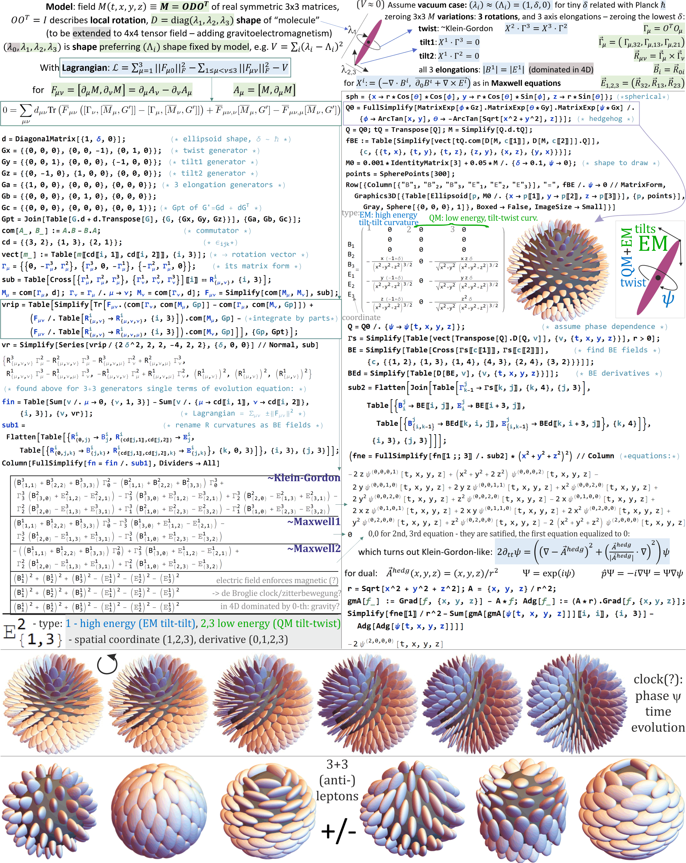
Figure 5: Used Mathematica source for 3D case and $\Lambda=(1,\delta,0)$ shape (available in https://github.com/JarekDuda/liquid-crystals-particle-models). Application of written evolution equation (35) $M_{\mu}$ in vacuum case ($V=0,G^{\prime}_{\mu}=0$), 6 generators $G$, and neglecting higher $\delta$ terms. Right: application for basic hedgehog case with $\psi$ function defining local twist (wavefunction $\Psi=\exp(i\psi)$), deriving Klein-Gordon-like equation. Bottom: visualization of expected phase evolution for de Broglie clock/zitterbewegung, and of 3 leptons, anti-leptons.

IV-B2 Simplification

: These equations for 3 generators $G$ are still quite complex. To simplify as in (16), denote 3x3 anti-symmetric matrices using $\vec{R}_{\mu\nu}=\vec{\Gamma}_{\mu}\times\vec{\Gamma}_{\nu}$ vectors. Then denote EB fields as coordinates of $R=F^{*}$ tensor:

$$\vec{B}_{1}=\vec{R}_{01}\qquad\vec{B}_{2}=\vec{R}_{02}\qquad\vec{B}_{3}=\vec{R}_{03}$$ (36)

$$\vec{E}_{1}=\vec{R}_{32}\qquad\vec{E}_{2}=\vec{R}_{13}\qquad\vec{E}_{3}=\vec{R}_{21}$$

each of them is now 3D vector, which coordinates correspond to different energies as in Fig. 4 - let us denote them with superscript e.g. $\vec{B}_{i}=(B_{i}^{1},B_{i}^{2},B_{i}^{3})$.

Let us now choose $\Lambda$ eigenvalues as $D=\textrm{diag}(1,\delta,0)$. For $\delta=0$ we get uniaxial nematic Faber’s case. Here we assume $\delta$ is tiny positive, with twist corresponding to quantum phase - hence $\delta$ should be related with Planck constant. Neglecting higher order $\delta$ terms, the 3 EB coordinates correspond to $\approx(1,\delta,\delta)$ energies: first coordinate $(B^{1}=(B^{1}_{1},B^{1}_{2},B^{1}_{3}),E^{1}=(E^{1}_{1},E^{1}_{2},E^{1}_{3}))$ to standard electromagnetism, the remaining two to low energy quantum phase, hopefully to recreate relativistic QM like Klein-Gordon, QED Lagrangian.

To find the final equations (35), neglecting higher order $\delta$ terms, there is provided used Mathematica source (GitHub, Fig. 5), leading to terms for 3 rotation generators:

$$\textrm{twist:}\quad\Gamma_{\mu}^{2}\partial_{\nu}R_{\mu\nu}^{3}-\Gamma_{\mu}^{3}\partial_{\nu}R_{\mu\nu}^{2}-\Gamma_{\nu}^{2}\partial_{\mu}R_{\mu\nu}^{3}+\Gamma_{\nu}^{3}\partial_{\mu}R_{\mu\nu}^{2}$$

$$\textrm{2 tilts:}\quad\Gamma_{\mu}^{3}\partial_{\nu}R_{\mu\nu}^{1}-\Gamma_{\nu}^{3}\partial_{\mu}R_{\mu\nu}^{1},\quad\Gamma_{\nu}^{2}\partial_{\mu}R_{\mu\nu}^{1}-\Gamma_{\mu}^{2}\partial_{\nu}R_{\mu\nu}^{1}$$

Such terms need to be summated by $\mu,\nu$ and equalized to 0, leading to Maxwell-like equation terms for EM. Denoting:

$$X^{i}=(-\nabla\cdot B^{i},\overrightarrow{\partial_{0}B^{i}+\nabla\times E^{i}}),$$ (37)

the (35) equations for 3 rotation generators become:

$$X^{2}\cdot\Gamma^{3}=X^{3}\cdot\Gamma^{2}\qquad\sim\textrm{Klein-Gordon for twist(phase)}$$ (38)

$$X^{1}\cdot\Gamma^{3}=0,\ X^{1}\cdot\Gamma^{2}=0\qquad\textrm{Maxwell equation for two tilts}$$

Figure 5 contains this implementation, also applying these equations to hedgehog ansatz (model of lepton), getting Klein-Gordon-like equation for the twist (phase). Figure 7 contains implementation deriving 4D equations, getting 2nd set of Maxwell-like equations for GEM. Figure 2 calculates Coulomb effective potential for such two topological charges, Figure 3 suggests a way to analogously get Newton law for 4D field.

Further work is planned to extend this agreement, also parametrization to moduli space, finally maybe hydrodynamical simulations. The first difficulty is getting angular momentum, clock for charge (electron), hopefully through regularization by including Higgs-like potential, as most of mass/energy of particle is localized in its center - where potential is nonzero.

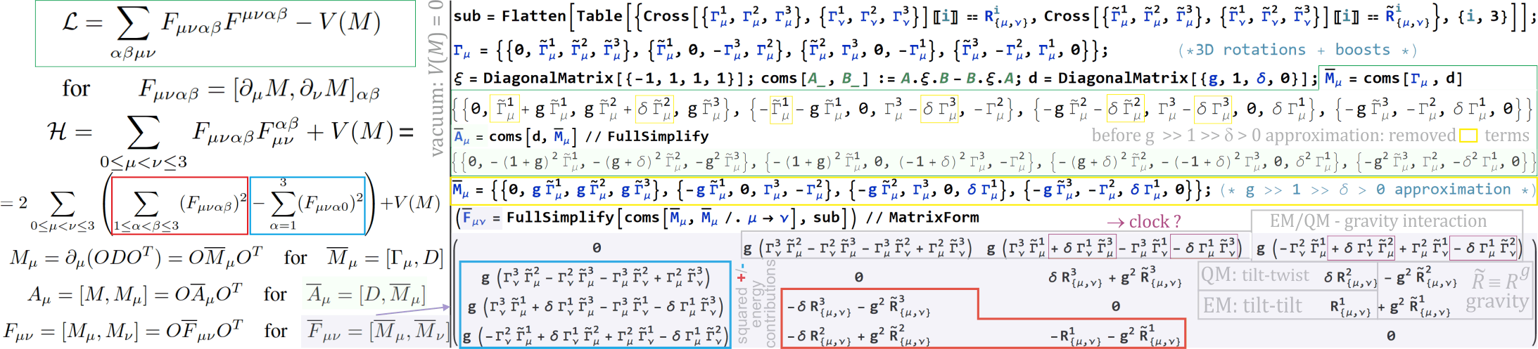
Figure 6: Gathered formulas for suggested 4D model, $M=ODO^{T}$, $D=\textrm{diag}(g,1,\delta,0)$ with calculated (in GitHub) vacuum $V(M)=0$, $g>>1>>\delta>0$ approximation for $\bar{F}_{\mu\nu}$. With tilde there are noted time axis/gravitational parts, $\vec{R}_{\mu\nu}=\vec{\Gamma}_{\mu}\times\vec{\Gamma}_{\nu}$. Surprisingly, the Hamiltonian turns out having not only positive (red), but also negative (blue) contributions. Positive energy contributions (red) for separate EM and GEM are as expected ($\sim E^{2}+B^{2}$), would lead to Maxwell equations for independent each of them. However, combined suggest tendency for opposite curvatures - nearly unsatisfied due to very rigid time axis direction (with tilde). The negative energy contributions (blue) give tendency to increase imbalance, such freedom is mostly in $\Gamma^{1}_{0}\tilde{\Gamma}_{i}$ for $i=1,2,3$ terms (violet) for temporal derivative of twist as in de Broglie clock, with rotation of temporal axis in spatial directions.

V 4D case: Lorentz invariance and gravity

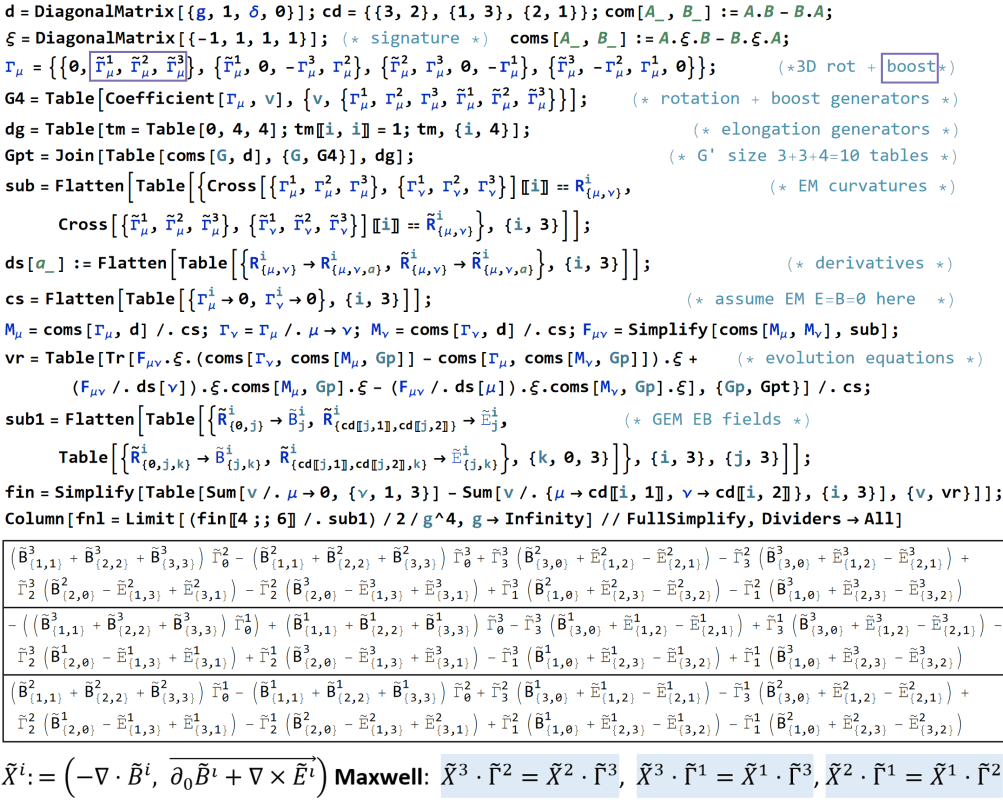
Figure 7: Basic source to derive equations for 4D case (available in GitHub) with $\Lambda=(g,1,\delta,0)$ shape and $g>>1$. Now we have 10 generators: 3 for 3D rotations corresponding to EM, 3 for boosts as rotations of 0th axis (symmetric vs antisymmetric generators) - leading to GEM, and 4 equations for elongations of 4 axes ($\tilde{\Gamma}\equiv\Gamma^{g},\tilde{R}\equiv R^{gg}$). Such equations become much more complex, there is derived GEM-only case with zeroed 3D rotations, getting Maxwell-like equations for GEM.

Previously we were focused on 3D case as for biaxial nematic, briefly mentioning 4D case e.g. as SO(4) rotation in (6). In contrast, there is a general belief for Lorentz invariance in 4D, replacing SO(4) with SO(1,3). The previous antisymmetric rotation generator (6) with mixed below - all positive $\vec{\Gamma}^{g}_{\mu}$ being boost generator for chosen rapidity:

$$\Gamma_{\mu}=O^{T}O_{\mu}=\left(\begin{array}[]{>{\columncolor{gray!20}}cccc}&\vec{\Gamma}^{g1}_{\mu}&\vec{\Gamma}^{g2}_{\mu}&\vec{\Gamma}^{g3}_{\mu}\\ \vec{\Gamma}^{g1}_{\mu}&0&-\vec{\Gamma}^{3}_{\mu}&\vec{\Gamma}^{2}_{\mu}\\ \vec{\Gamma}^{g2}_{\mu}&\vec{\Gamma}^{3}_{\mu}&0&-\vec{\Gamma}^{1}_{\mu}\\ \vec{\Gamma}^{g3}_{\mu}&-\vec{\Gamma}^{2}_{\mu}&\vec{\Gamma}^{1}_{\mu}&0\\ \end{array}\right)$$ (39)

Matrix $O\equiv O_{\alpha}^{\beta}$ contains rotation and boost, is no longer orthogonal, but still we can use $M=ODO^{T}$, can be calculated by exponentiation of above generator matrix.

In Euler-Lagrange equations for vacuum we should use 6 generators: 3 antisymmetric for 3D rotation (24), and 3 symmetric for boosts (+ 4 axis elongation generators):

$$\left(\begin{array}[]{cccc}0&1&0&0\\ 1&0&0&0\\ 0&0&0&0\\ 0&0&0&0\\ \end{array}\right),\left(\begin{array}[]{cccc}0&0&1&0\\ 0&0&0&0\\ 1&0&0&0\\ 0&0&0&0\\ \end{array}\right),\left(\begin{array}[]{cccc}0&0&0&1\\ 0&0&0&0\\ 0&0&0&0\\ 1&0&0&0\\ \end{array}\right)$$

Another change is in matrix products - they are unchanged for $O\equiv O_{\alpha}^{\beta}$ up-down indexes. However, our fundamental tensor field is rather symmetric as $M\equiv M_{\alpha\beta}$ (equivalently could be both upper indexes), requiring $M_{\alpha\beta}\to M_{\alpha}^{\beta}$ by product with $\xi=\textrm{diag}(-1,1,1,1)$ spacetime signature matrix, e.g. transforming:

$$[M_{\mu},M_{\nu}]\to M_{\mu}\xi M_{\nu}-M_{\nu}\xi M_{\mu}\qquad\textrm{for}\quad\xi=\textrm{diag}(-1,1,1,1)$$ (40)

For Lagrangian we further took Frobenius norm of such commutator, which for Lorentz invariance becomes:

$$\|X\|^{2}_{F}\to\|X\|_{\xi}^{2}:=\textrm{Tr}(X\xi X^{T}\xi)=\sum_{\mu\nu}X_{\mu\nu}X^{\mu\nu}$$ (41)

with also negative contributions, well known e.g. in EM Lagrangian:

$$\|F\|_{\xi}^{2}=\sum_{\mu\nu}F_{\mu\nu}F^{\mu\nu}=2\sum_{1\leq\mu<\nu\leq 3}\left(F_{\mu\nu}\right)^{2}-2\sum_{\mu=1}^{3}\left(F_{0\mu}\right)^{2}$$

Finally Lorentz invariant Lagrangian can be chosen as (we can use $[\partial_{\mu}M,\partial_{\nu}M]=\partial_{\mu}M\,\xi\,\partial_{\nu}M-\partial_{\nu}M\,\xi\,\partial_{\mu}M$ operating on matrices):

$$\mathcal{L}=\sum_{\alpha\beta\mu\nu}F_{\mu\nu\alpha\beta}F^{\mu\nu\alpha\beta}-V(M)$$ (42)

$$\textrm{for}\qquad F_{\mu\nu\alpha\beta}=[\partial_{\mu}M,\partial_{\nu}M]_{\alpha\beta}$$

with electromagnetic $F$ tensor extended to include also quantum phase governed by Klein-Gordon-like equation, and second set of Maxwell equations for gravity.

Figure 6 contains practical approximation of $\bar{F}_{\mu\nu}$ tensor with as $F_{\mu\nu}$ with reversed rotation and boost. It is for vacuum case with $D=\textrm{diag}(g,1,\delta,0)$ shape for $g>>1>>\delta>0$ formula (16) for $O$ containing rotation + boost and $\Gamma_{\mu}=O^{T}O_{\mu}$. The $\Gamma,R\equiv R^{e}$ are for spatial rotations, $\tilde{\Gamma},\tilde{R}\equiv R^{g}$ for the 0th time axis.

Hamiltonian can be calculated as previously (23), replacing Frobenius norm with Lorentz invariant one - having both positive spatial energy contributions, but surprisingly also negative $\alpha 0$ energy contributions (as Legendre transform changes only 2 out of 4 indexes of curvature tensor - corresponding to derivation directions, not SO(1,3) generators inside):

$$\mathcal{H}=\sum_{0\leq\mu<\nu\leq 3}F_{\mu\nu\alpha\beta}F_{\mu\nu}^{\alpha\beta}+V(M)$$ (43)

$$\mathcal{H}=2\sum_{0\leq\mu<\nu\leq 3}\left(\sum_{1\leq\alpha<\beta\leq 3}(F_{\mu\nu\alpha\beta})^{2}-\sum_{\alpha=1}^{3}(F_{\mu\nu\alpha 0})^{2}\right)+V(M)$$

Spatial part of $\bar{F}_{\mu\nu}$ in Figure 6 contains sum of spatial curvature, as previously (e.g. Fig. 4) multiplied by $\delta$ for 2nd and 3rd coordinate (without $R^{1}_{\mu\nu}=\Gamma^{2}_{\mu}\Gamma^{3}_{\nu}-\Gamma^{3}_{\mu}\Gamma^{2}_{\nu}$). It is summed with curvature of time axis $R^{g}\equiv\tilde{R}$ corresponding to GEM. Energy density (Hamiltonian) contains squares of such sums, giving them tendency to get opposite signs. However, dynamics of time axis is much more rigid - $R^{g}$ can be assumed as locally nearly constant for EM, in practice averages of EM/QM influence time axis.

The most interesting are negative energy contributions to Hamiltonian, corresponding to interaction of spatial and temporal dynamics, giving tendency to increase their imbalance. The $\Gamma^{1}_{0}\tilde{\Gamma}_{i}$ terms for $i=1,2,3$ have large freedom for such imbalance - time derivative of twist (”quantum phase”) and rotations of time axis, bringing hope for propulsion of de Broglie clock/zitterbewegung phase evolutions of particles.

However, the details are very complex, will need further work. The negative energy term should be usually compensated by positive, unless e.g. lack of charges nearby - what might explain dark matter/energy, believed to contain e.g. $\sim 95\%$ of energy. Obviously the discussed Lagrangian might be incorrect, or simplified e.g. requiring additional terms.

Regarding the Higgs-like potential $V(M)$ minimized for a fixed set of eigenvalues (shape), one approach could be like Landau-de Gennes using traces of powers, now we need to modify it for SO(1,3) to include rotations and boosts. Using $M\equiv M_{\alpha\beta}$, traces of $(M\xi)^{p}=(-\lambda_{0})^{p}+\lambda_{1}^{p}+\lambda_{2}^{p}+\lambda_{3}^{p}$ are rotation-boost invariants, we could use e.g. $V(M)=\sum_{p=1}^{k}(\textrm{Tr}((M\xi)^{p})-c_{p})^{2}$ potential. Choosing its details is very difficult, will rather require PDE simulations.

VI Conclusions and further work

There was briefly presented mathematical framework allowing for EM + pilot wave + GEM unification for topological configurations e.g. in (superfluid) liquid crystals, extending Faber’s approach: vectors $\to$ matrices, to make $\Gamma,R$ now include shape dependence becoming $A,F$, this way distinguishing EM $>>$ QM $>>$ GEM vacuum dynamics.

This article is work in progress, which is planned to be further developed: aiming as good agreement with particle physics as possible - both for better understanding, also maybe to try to recreate some phenomena with liquid crystal experiments, like observation of additional fluxon-like vortex for hedgehog configuration in biaxial nematic (no naked charges), transformation between 3 types of vortices as neutrino oscillation analogy.

One main open question is choosing the potential - e.g. depending only on the shape $V(M)$, or maybe also derivatives $V(A)$, ideally with minimal number of parameters like only preferred eigenvalues (or less). A natural direction is through search for agreement with 3 leptons as hedgehog of one of 3 axes as in Fig. 1: they should form 3 local minima in the space of possible rotations of hedgehog ansatz, probably stabilized by the enforced magnetic vortices.

Ideally e.g. electron configuration should also enforce intrinsic periodic process (zitterbewegung/de Broglie clock [18]) e.g. as rotation of additional degree of freedom for uniaxial $\to$ biaxial transition, what could be obtained by regularization or 4D formulation adding gravitational mass in obtained Klein-Gordon-like equation. Details are yet to be developed, e.g. gravitational mass might require e.g. fixing $\det(M)$ constraint suggested in [32]. EM-GEM interaction slowing down EM propagation could explain graviational time dilation and lensing.

Calculations like started in Fig. 2, 3, 5 and 7 are crucial development direction, also parametrizations to moduli space, trying to extend correspondence with particle physics, finally performing 2nd quantization aiming agreement with the standard model. Preferably also full hydrodynamical simulations to better understand the configurations and dynamics.

Finally, there is huge menagerie of particles - the big question is which can be obtained with this kind of approach, ideally would be getting all with proper dynamics, after 2nd quantization agreeing with the Standard Model. There are promising topological soliton approaches for nuclei [37], using topological number as baryon number instead of electric charge here. Qualitative suggestion for further particles with approach discussed here can be found in [38] and is sketched in Fig. 8, is planned to be verified, developed in the future.

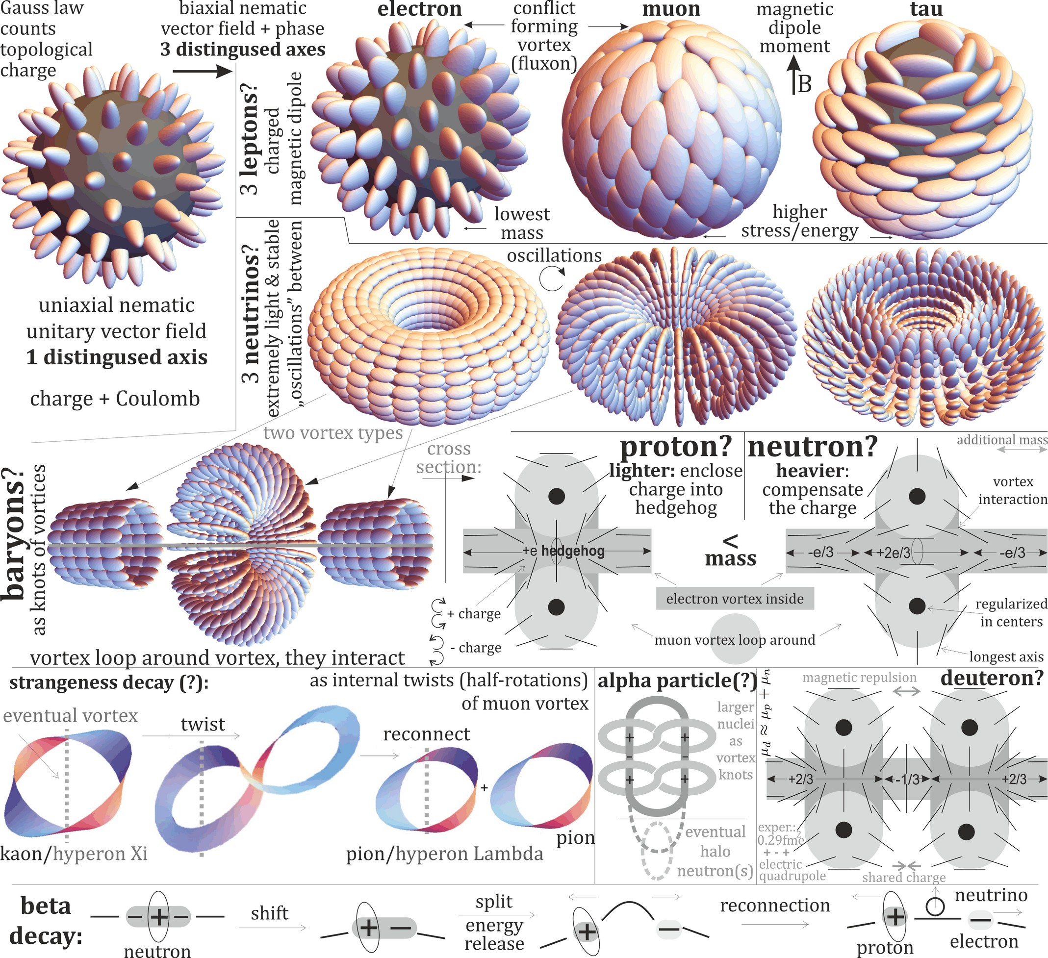
Figure 8: Possible directions to get further particle-like configurations for biaxial nematic-like systems. Hedgehog configurations of one of 3 axes resemble 3 leptons: the same electric charge (as topological), but different realization: regularization, mass. Hairy ball theorem says there is a conflict of axes on the sphere - leading to outgoing vortex (2D topological charge) of one of 3 types (along one of 3 axes) - like fluxons in superconductor carrying magnetic field: enforcing magnetic dipole moment. Short loop of such vortex would be very light and difficult to interact with, resembling 3 neutrinos - with possible oscillations between each other through field rotation, they should be produced in beta decay. Such vortices, resembling ”quark strings” in QCD, can further form knots, which resemble baryons, nuclei. Interaction between vortices inside such knot with vortex loop around enforces charge-like (hedgehog) configuration inside: makes that baryon configuration requires some charge - can be fractional, but all sum to integer charge (confinement). Proton can just enclose this charge (hedgehog), but neutron has to compensate it to zero - suggesting why neutron is heavier (naively should be lighter due to charge), through quark-like fractional charge structure. Such concluded: positive core, negative shell charge distribution of neutron is suggested in literature e.g. [40]. It also suggest binding mechanism for deuteron: as two baryons sharing required charge - also explaining observed relatively large electric quadrupole moment (experimentally: 0.2859 e $\textrm{fm}^{2}$) and aligned spins $(\mu_{d}\approx\mu_{p}+\mu_{n})$. Binding of larger nuclei could additionally use vortices forming stable knots, e.g. halo nuclei with neutrons stably bind in large a few femtometer distance. Vortex loop might have additional internal twist, which is quantized ($k\pi/2$) and resembles strangeness - relaxed through muon/kaon production in decay of strange baryons.

References

• [1] R. Ruhwandl and E. Terentjev, “Long-range forces and aggregation of colloid particles in a nematic liquid crystal,” Physical Review E, vol. 55, no. 3, p. 2958, 1997.
• [2] P. Poulin, H. Stark, T. Lubensky, and D. Weitz, “Novel colloidal interactions in anisotropic fluids,” Science, vol. 275, no. 5307, pp. 1770–1773, 1997.
• [3] B.-K. Lee, S.-J. Kim, J.-H. Kim, and B. Lev, “Coulomb-like elastic interaction induced by symmetry breaking in nematic liquid crystal colloids,” Scientific reports, vol. 7, no. 1, pp. 1–8, 2017.
• [4] Y. Shen and I. Dierking, “Annihilation dynamics of topological defects induced by microparticles in nematic liquid crystals,” Soft matter, vol. 15, no. 43, pp. 8749–8757, 2019.
• [5] M. Faber, “Model for topological fermions,” Few-Body Systems, vol. 30, no. 3, pp. 149–186, 2001.
• [6] M. Faber and A. P. Kobushkin, “Electrodynamic limit in a model for charged solitons,” Physical Review D, vol. 69, no. 11, p. 116002, 2004.
• [7] M. Faber, “Particles as stable topological solitons,” in Journal of Physics: Conference Series, vol. 361, no. 1.   IOP Publishing, 2012, p. 012022.
• [8] ——, “A geometric model in 3+ 1d space-time for electrodynamic phenomena,” Universe, vol. 8, no. 2, p. 73, 2022.
• [9] J. Wabnig, J. Resch, D. Theuerkauf, F. Anmasser, and M. Faber, “Numerical evaluation of a soliton pair with long range interaction,” arXiv preprint arXiv:2210.13374, 2022.
• [10] A. Becciu, A. Fuster, M. Pottek, B. van den Heuvel, B. ter Haar Romeny, and H. van Assen, “3d winding number: Theory and application to medical imaging,” International journal of biomedical imaging, vol. 2011, 2011.
• [11] P.-G. De Gennes and J. Prost, The physics of liquid crystals.   Oxford university press, 1993, no. 83.
• [12] E. F. Gramsbergen, L. Longa, and W. H. de Jeu, “Landau theory of the nematic-isotropic phase transition,” Physics Reports, vol. 135, no. 4, pp. 195–257, 1986.
• [13] J.-S. B. Tai, “Topological solitons in chiral condensed matters,” Ph.D. dissertation, University of Colorado at Boulder, 2020.
• [14] M. Berry, R. Chambers, M. Large, C. Upstill, and J. Walmsley, “Wavefront dislocations in the Aharonov-Bohm effect and its water wave analogue,” European Journal of Physics, vol. 1, no. 3, p. 154, 1980.
• [15] F. Vivanco, F. Melo, C. Coste, and F. Lund, “Surface wave scattering by a vertical vortex and the symmetry of the Aharonov-Bohm wave function,” Physical review letters, vol. 83, no. 10, p. 1966, 1999.
• [16] A. Eddi, J. Moukhtar, S. Perrard, E. Fort, and Y. Couder, “Level splitting at macroscopic scale,” Physical review letters, vol. 108, no. 26, p. 264503, 2012.
• [17] M. Eisenberg and R. Guy, “A proof of the hairy ball theorem,” The American Mathematical Monthly, vol. 86, no. 7, pp. 571–574, 1979.
• [18] P. Catillon, N. Cue, M. Gaillard, R. Genre, M. Gouanère, R. Kirsch, J.-C. Poizat, J. Remillieux, L. Roussel, and M. Spighel, “A search for the de broglie particle internal clock by means of electron channeling,” Foundations of Physics, vol. 38, no. 7, pp. 659–664, 2008.
• [19] C. Qu, C. Hamner, M. Gong, C. Zhang, and P. Engels, “Observation of Zitterbewegung in a spin-orbit-coupled Bose-Einstein condensate,” Physical Review A, vol. 88, no. 2, p. 021604, 2013.
• [20] M. Gryziński, “Spin-dynamical theory of the wave-corpuscular duality,” International Journal of Theoretical Physics, vol. 26, no. 10, pp. 967–980, 1987.
• [21] Y. Couder and E. Fort, “Single-particle diffraction and interference at a macroscopic scale,” Physical review letters, vol. 97, no. 15, p. 154101, 2006.
• [22] A. Eddi, E. Fort, F. Moisy, and Y. Couder, “Unpredictable tunneling of a classical wave-particle association,” Physical review letters, vol. 102, no. 24, p. 240401, 2009.
• [23] E. Fort, A. Eddi, A. Boudaoud, J. Moukhtar, and Y. Couder, “Path-memory induced quantization of classical orbits,” Proceedings of the National Academy of Sciences, vol. 107, no. 41, pp. 17 515–17 520, 2010.
• [24] S. Perrard, M. Labousse, M. Miskin, E. Fort, and Y. Couder, “Self-organization into quantized eigenstates of a classical wave-driven particle,” Nature communications, vol. 5, no. 1, pp. 1–8, 2014.
• [25] D. M. Harris, J. Moukhtar, E. Fort, Y. Couder, and J. W. Bush, “Wavelike statistics from pilot-wave dynamics in a circular corral,” Physical Review E, vol. 88, no. 1, p. 011001, 2013.
• [26] B. C. Denardo, J. J. Puda, and A. Larraza, “A water wave analog of the Casimir effect,” American Journal of Physics, vol. 77, no. 12, pp. 1095–1101, 2009.
• [27] I. M. Pop, B. Douçot, L. Ioffe, I. Protopopov, F. Lecocq, I. Matei, O. Buisson, and W. Guichard, “Experimental demonstration of aharonov-casher interference in a josephson junction circuit,” Physical Review B, vol. 85, no. 9, p. 094503, 2012.
• [28] A. Shnirman, E. Ben-Jacob, and B. Malomed, “Tunneling and resonant tunneling of fluxons in a long josephson junction,” Physical Review B, vol. 56, no. 22, p. 14677, 1997.
• [29] Y. Aharonov, S. Nussinov, S. Popescu, and B. Reznik, “Aharonov-bohm type forces between magnetic fluxons,” Physics Letters A, vol. 231, no. 5-6, pp. 299–303, 1997.
• [30] V. V. Nesvizhevsky, H. G. Börner, A. K. Petukhov, H. Abele, S. Baeßler, F. J. Rueß, T. Stöferle, A. Westphal, A. M. Gagarski, G. A. Petrov et al., “Quantum states of neutrons in the earth’s gravitational field,” Nature, vol. 415, no. 6869, pp. 297–299, 2002.
• [31] Z. Burda, J. Duda, J.-M. Luck, and B. Waclaw, “Localization of the maximal entropy random walk,” Physical review letters, vol. 102, no. 16, p. 160602, 2009.
• [32] J. Duda, “Four-dimensional understanding of quantum mechanics,” arXiv preprint arXiv:0910.2724, 2009.
• [33] ——, “Extended maximal entropy random walk,” Ph.D. dissertation, Jagiellonian University, 2012. [Online]. Available: http://www.fais.uj.edu.pl/documents/41628/d63bc0b7-cb71-4eba-8a5a-d974256fd065
• [34] ——, “Diffusion models for atomic scale electron currents in semiconductor, pn junction,” arXiv preprint arXiv:2112.12557, 2021.
• [35] G. E. Volovik, The universe in a helium droplet.   Oxford University Press on Demand, 2003, vol. 117.
• [36] N. Manton and P. Sutcliffe, Topological solitons.   Cambridge University Press, 2004.
• [37] C. Naya and P. Sutcliffe, “Skyrmions and clustering in light nuclei,” Physical review letters, vol. 121, no. 23, p. 232002, 2018.
• [38] J. Duda, “Topological solitons of ellipsoid field-particle menagerie correspondence,” 2012. [Online]. Available: http://fqxi.org/community/forum/topic/1416
• [39] A. A. Abrikosov, “The magnetic properties of superconducting alloys,” Journal of Physics and Chemistry of Solids, vol. 2, no. 3, pp. 199–208, 1957.
• [40] S. Haddad and S. Suleiman, “Neutron charge distribution and charge density distributions in lead isotopes,” Acta Physica Polonica B, vol. 30, no. 1, p. 119, 1999.
Refer to caption