Characterizing multistability regions in the parameter space of the Mackey-Glass delayed system

Abstract

Proposed to study the dynamics of physiological systems in which the evolution depends on the state in a previous time, the Mackey-Glass model exhibits a rich variety of behaviors including periodic or chaotic solutions in vast regions of the parameter space. This model can be represented by a dynamical system with a single variable obeying a delayed differential equation. Since it is infinite dimensional requires to specify a real function in a finite interval as an initial condition. Here, the dynamics of the Mackey-Glass model is investigated numerically using a scheme previously validated with experimental results. First, we explore the parameter space and describe regions in which solutions of different periodic or chaotic behaviors exist. Next, we show that the system presents regions of multistability, i.e. the coexistence of different solutions for the same parameter values but for different initial conditions. We remark the coexistence of periodic solutions with the same period but consisting of several maximums with the same amplitudes but in different orders. We characterize the multistability regions by introducing families of representative initial condition functions and evaluating the abundance of the coexisting solutions. These findings contribute to describe the complexity of this system and explore the possibility of possible applications such as to store or to code digital information.

1 Introduction

The Mackey-Glass (MG) model was first introduced to model respiratory and hematopoietic diseases related to physiological systems mackey1977oscillation . Perhaps the most remarkable characteristic of this model is that the evolution of the system depends on the state in a previous, or delayed, time. MG model obtained great recognition thanks to its ability to accurately describe in simple terms complicated dynamics such as a variety of human illnesses belair1995dynamical . Nonetheless, the relevance of the MG model goes beyond its application to specific systems and results illuminating in a broad variety of delayed systems biswas2018time exhibiting chaotic behaviour and multistability.

Delayed systems are in general considerably more complicated than non-delayed. Even in the simplest case of a single delay, $tau$, the evolution of the system at present time $t$ depends on the state at time $t-\tau$, thus, it also depends on a infinite set of previous times, $t-\tau$, $t-2\tau$, …. These systems are infinite dimensional and mathematically they can be represented by systems of delayed differential equations (DDE). In this sense these equations are far more complex than ODEs and behave like infinite-dimensional systems of ODEs hale2013introduction . Moreover, the dynamics of DDEs are far more rich than those of ODEs. For instance, the peculiar routes to chaos, or the creation and destruction of isolated peaks in the MG system have been detailed studied by Junges and Gallas junges2012intricate .

The presence of multistability in the MG model, i.e. several coexisting solutions for the same parameter values but different initial conditions, was reported by losson1993solution . This coexistence of solutions of a time-delayed feedback system could be of practical interest. In particular, it was proposed as an alternative way for storing information mensour1995controlling ; lim1998experimental ; zhou2007isochronal . The ability to synchronize several coupled MG systems is also relevant and has received considerable attention in the last years pyragas1998synchronization ; kim2006synchronization ; shahverdiev2006chaos .

In addition to numerical studies, different experimental systems based on electronic implementations that mimic the MG model were proposed namajunas1995electronic ; amil2015exact . Due to the analytical and numerical difficulties, experimental results play a major role and contribute to validate theoretical models. In particular, experimental observations can shed light on the feasibility of the observed solutions under the presence of noise or parameter mismatch. Recently, an electronic system mimicking the dynamics of the MG system, whose central elements are a bucket bridge device (BBD) and a nonlinear function block, was proposed by Amil et al. amil2015exact . A remarkable characteristic of this approach is that the temporal integration is exact, thus, experimental and numerical simulations agree very well with each other enabling the study of large regions in the parameter space. In a subsequent investigation amil2015organization , this approach was used to explore the parameter space described in terms of the dimensionless delay and production rate. This study unmasked the existence of periodic and chaotic solutions intermingled in vast regions of the parameter space. A remarkable point is the existence of abundant solutions with the same period but consisting of several peaks with the same amplitudes but in different alternations. These periodic solutions can be translated to sequences of letters and classified using symbolic algorithms.

In spite of these extensive studies, there are still numerous open questions, in particular, in which regions of the parameter space the system presents multistability and where the coexistence of solutions is more abundant. Here we report the presence of tongue-like structures of stability in the midst of chaotic regions in the parameter space and that these solutions seem to retain some of their structure inside these regions of stability. We also go deeper into the organization of the solutions and the impact of multistability. Given that there are infinite initial condition functions, we select a specific family of functions as a proxy to quantitatively evaluate the strength of the multistabilty. Our study shows that, although there are some general trends, there exist regions in which the coexistence is clearly more noticeable than in others. The rest of this work is organized as follows. In the next Section we shortly summarize the basic ingredient of the model and review the numerical methods used. In Section 3 we numerically explore the parameter space identifying the most interesting regions. The analysis of the multistability and the abundance of coexistent solutions with the same parameter values but different initial conditions is presented in Section 4. Finally, Section 5 is devoted to the final remarks.

2 The MG model and the numerical method

The original model describes the dynamics of a physiological variable, $P(t)$ representing the concentration of a particular cell population in the blood. The temporal evolution is governed by the following equation

$$\frac{dP}{dt}=\frac{\beta_{0}\theta^{n}P_{\tau}}{\theta^{n}+P_{\tau}^{n}}-\gamma P$$ (1)

where $P_{\tau}=P(t-\tau)$ is the delayed variable and $\beta_{0}$, $\theta$, $\tau$, $n$, $\gamma$ are real parameters mackey1977oscillation . In this equation the first term in the right hand side represents the nonlinear, delayed, production and the second term accounts for the natural decaying. The number of parameters can be reduced by re-scaling the variables $x=P/\theta$ and $t^{\prime}=\gamma t$ in Eq. (1) obtaining,

$$\frac{dx}{dt^{\prime}}=\alpha\frac{x_{\Gamma}}{1+x_{\Gamma}^{n}}-x$$ (2)

where $x_{\Gamma}=x(t^{\prime}-\Gamma)$, $\alpha=\beta_{0}/\gamma$ and $\Gamma=\gamma\tau$. From now on we denote the re-scaled time simply as $t$.

The temporal evolution of the dimensionless variable $x(t)$ is given by Eq. (2) which is the center of our analysis. This equation depends on three parameters: $n$, $\alpha$, and $\Gamma$. The first one, $n$ is directly related to the mechanism of production of the particular blood component and it is kept fixed at $n=4$ through all this work. The other two parameters, $\alpha$ and $\Gamma$, correspond to the production rate and the decay and we will take them as the main variables of the control or parameter space. In this DDE with a single delay, the initial condition must specify a function in the interval $(-\Gamma,0)$ to univocally determine the solution $x(t)$.

The numerical integration of the DDE requires to redesign a standard numerical methods for ordinary differential equations smith2011introduction . The first alternative is to appeal to standard numerical methods, like Runge-Kutta schemes with constant step-size, and store at each step the previous values of the variables in an interval at least equal to the maximum delay. Moreover, in the first steps during a time lapse at least equal to the maximum delay it is necessary to rely on another method to advance. In general, this approach is not the most efficient and it is difficult to verify the stability and accuracy. Other methods to solve DDEs numerically include the Bellman’s method of steps and wave relaxation methods as shown in bellen2013numerical .

In a very different approach amil2015exact , we proposed an electronic system that reproduces MG model. Moreover, we showed that taking into account the specific expressions for the nonlinear function and the delay block an explicit discretization scheme can be derived. This scheme presents the advantage that in addition to being more natural and easier to implement than standard methods the temporal evolution is exact in time.

This exact discretization of the Mackey-Glass equation amil2015exact can be obtained by taking discrete times $t_{j}=jdt$, where $dt$ is the sampling time. The number of values stored in the BBD, $N$ (in this work, N=1194), the time delay, $\Gamma$ and the sampling time are related through $dt=\Gamma/N$. The MG variable $x(t)$ is also discretized as $x_{j}$ whose temporal evolution is governed by the following equation

$$x_{j+1}=x_{j}e^{-\frac{\Gamma}{N}}+\Big{(}1-e^{-\frac{\Gamma}{N}}\Big{)}\frac{\alpha x_{j-N+1}}{1+x_{j-N+1}}.$$ (3)

It can be shown that this numerical method based on the exact discretization is a reliable representation of the experimental electronic system and a good approximation of Eq. (2) for sufficiently large values of $N$, as well as being more efficient than standard numerical algorithms amil2015exact ; amil2015organization .

3 Exploring the parameter space

As mentioned, the Mackey-Glass system exhibits a rich variety of dynamics depending on the parameters: the nonlinear function exponent $n$, the production rate, $\alpha$, and the delay $\Gamma$, and also on the initial condition function. We start considering temporal series for representative values of the delay, $\Gamma=15,25,35$ and $\alpha=4,6,8$ while the initial condition function and the exponent $n$ are kept fixed. In Fig. 1 the temporal series shown exhibit periodic behaviour for $\alpha=6$ and $\alpha=8$ for all $\Gamma$ values. The number of peaks per period is 30, 25 and 35 for the top series and 29, 22 and 28 for the ones in the middle. The bottom series, corresponding to $\alpha=4$, are all chaotic. We observe that series in the same row reveal different period while their shape changes abruptly. In this case, $T=125.9$, $T=102.9$ and $T=142.9$, for $\Gamma=15$, $\Gamma=25$ and $\Gamma=35$ respectively. The creation and destruction of peaks manifested in series along the same column is clear where the temporal series present the same period but different peaks count (indicated in each panel).

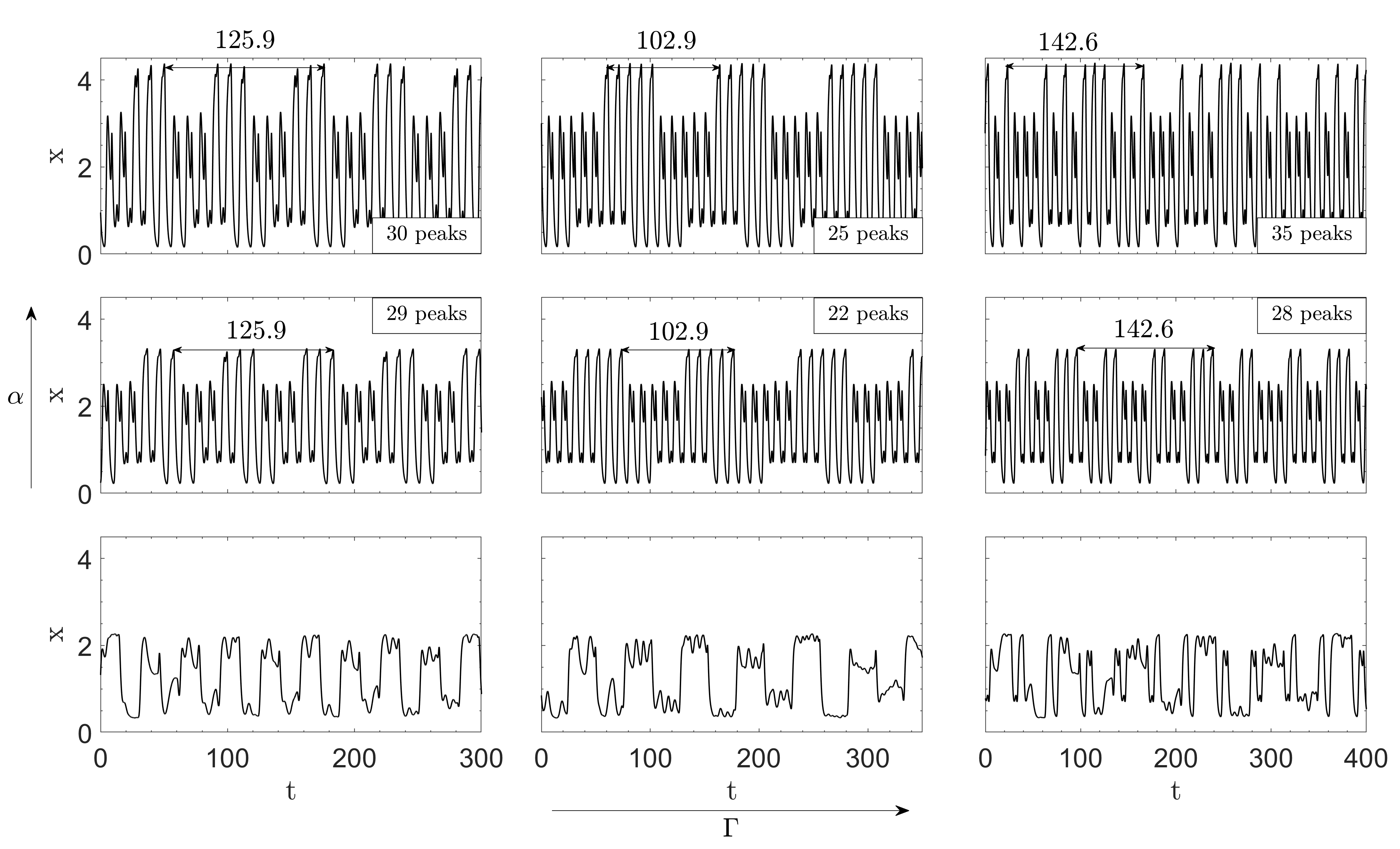
Figure 1: Time series evolution as control parameters $\alpha$ and $\Gamma$ are varied. Columns correspond to $\Gamma=[15,25,35]$ from left to right and rows correspond to $\alpha=[4,6,8]$ from bottom to top. A transient time of $5000\Gamma$ was neglected. In all the panels, initial conditions were set to $x_{in}(t)=1$ $\forall t\in(-\Gamma,0)$.

Figure 2 shows bifurcation diagrams obtained by plotting the local maximums (peaks) of the numerically computed solutions as a function of $\Gamma$ for three different values of $\alpha$. In all the cases, the initial condition functions is $x_{in}(t)=1$ in the interval $(-\Gamma,0)$. These diagrams show the familiar periodic branches and chaotic behaviour. For $\alpha=4$ and $\Gamma<8$, typical period-doubling branches are exhibited, and the system presents a no return to periodicity for $\Gamma>8$. For $\alpha=6$ and $\alpha=8$ three different periodic regions are observed after the first transition to chaos. Creation and destruction of branches is also evident in Fig. 2 for all three diagrams, which is typical of delayed systems. All periodic regions appear similar inside the diagrams even as the delay parameter $\Gamma$ is increased. The diagrams also reveals regions of periodic solutions with similar peak structures for a range of values of $\alpha$. In general, complex arrangements appear for high $\Gamma$ values as $\alpha$ is increased. For example the creation of a high number of spontaneous branches is shown for $\Gamma=30$ and $\alpha=8$.

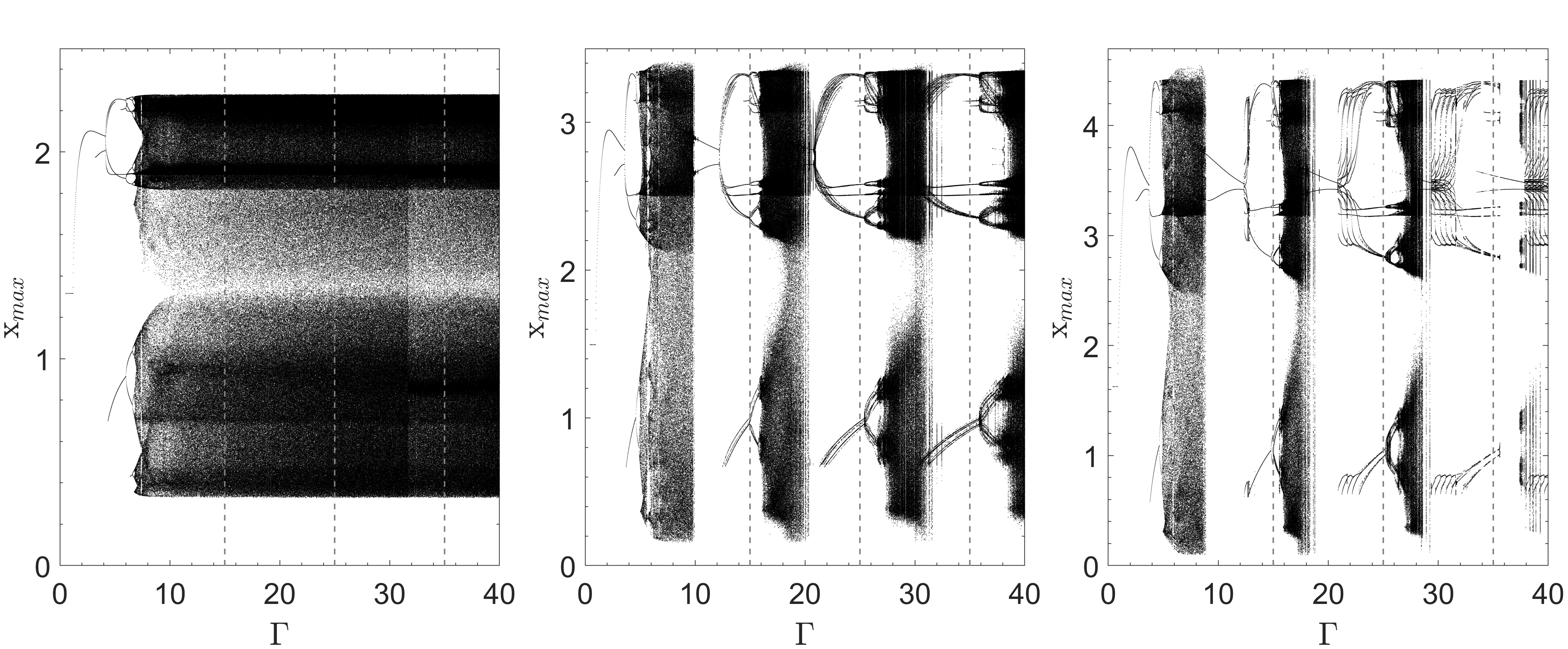
Figure 2: Bifurcation diagrams for different values $\alpha=4$ (left panel), $\alpha=6$ (center panel) and $\alpha=8$ (right panel). Peaks are recorded in a span of $200\Gamma$ after a transient of $5000\Gamma$ was neglected. Initial conditions were set to $x_{in}(t)=1$ $\forall t\in(-\Gamma,0)$. Vertical dashed lines correspond to the parameter values of Fig. 1.

Figure 3 shows bifurcation diagrams where parameter $\Gamma$ was swept up (top row) and down (bottom row) using the previous solution as the initial condition (the first initial condition function is $x_{in}(t)=1$ in the interval $(-\Gamma,0)$). The three columns correspond to different values of $\alpha$. Similar behaviour to that observed in Fig. 2 concerning that of period-doubling and creation and destruction of branches is noticed, but in Fig. 3 periodic solutions appear for $\alpha=4$ and $\Gamma>8$ whereas in Fig. 2 that region was entirely chaotic, evidencing the multistability of the system. Furthermore, the differences between the top and bottom row diagrams suggest a sort of hysteresis loop since the diagrams vary as $\Gamma$ is swept up or down. This hysteresis phenomena is further hint of the multistability of the system as the initial conditions are not the same when sweeping $\Gamma$ up to those when sweeping $\Gamma$ down.

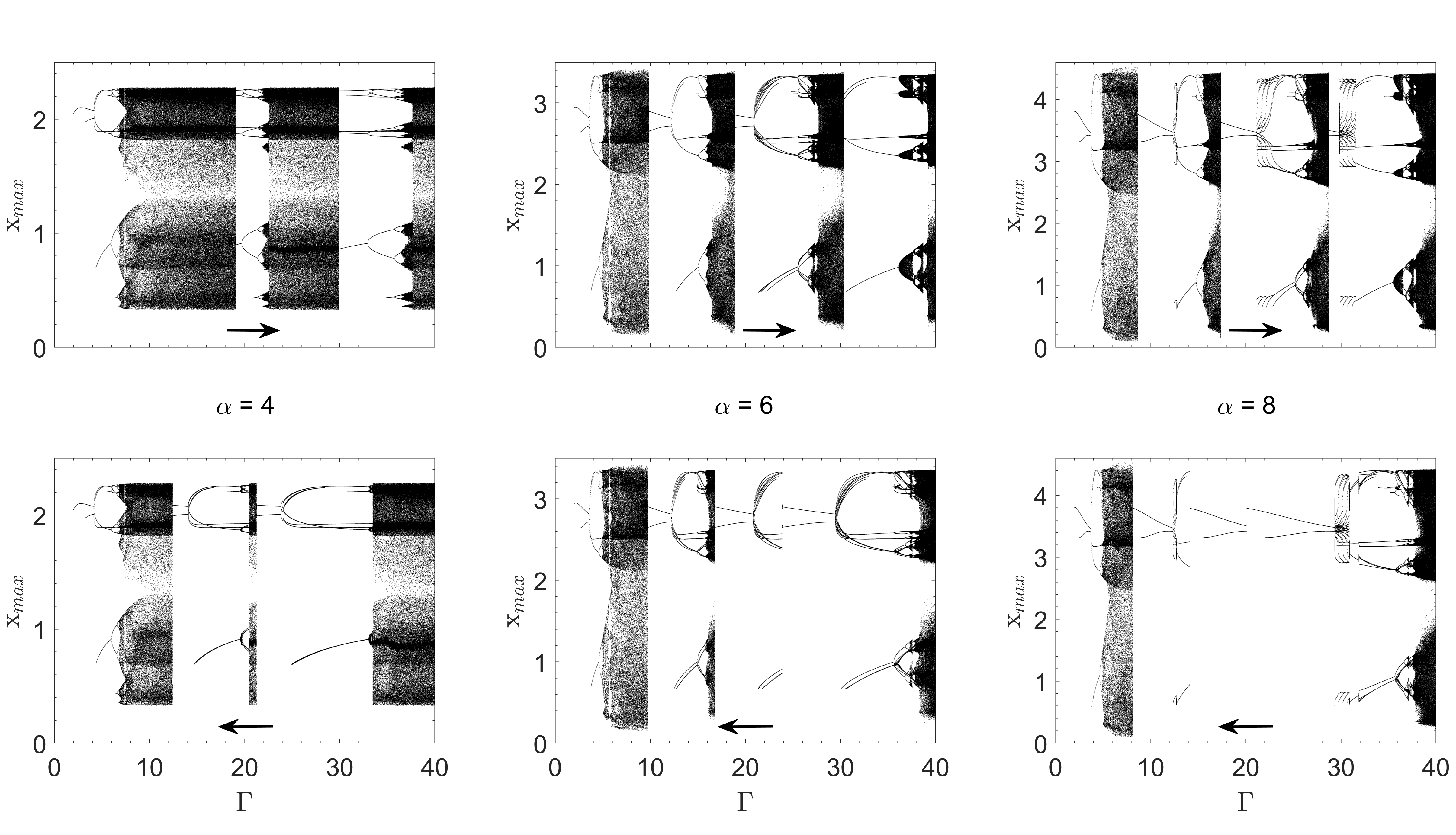
Figure 3: Bifurcation diagrams for different values $\alpha=4$ (left column), $\alpha=6$ (center column) and $\alpha=8$ (right column). Peaks are recorded in a span of $200\Gamma$ after a transient of $2000\Gamma$ was neglected. The initial condition for $\Gamma=2$ was set to $x_{in}(t)=1$ $\forall t\in(-\Gamma,0)$, then the previous solution was used as the initial condition as $\Gamma$ was swept up and then down. The top row corresponds to sweeping $\Gamma$ up whereas the bottom row correspond to sweeping $\Gamma$ down.

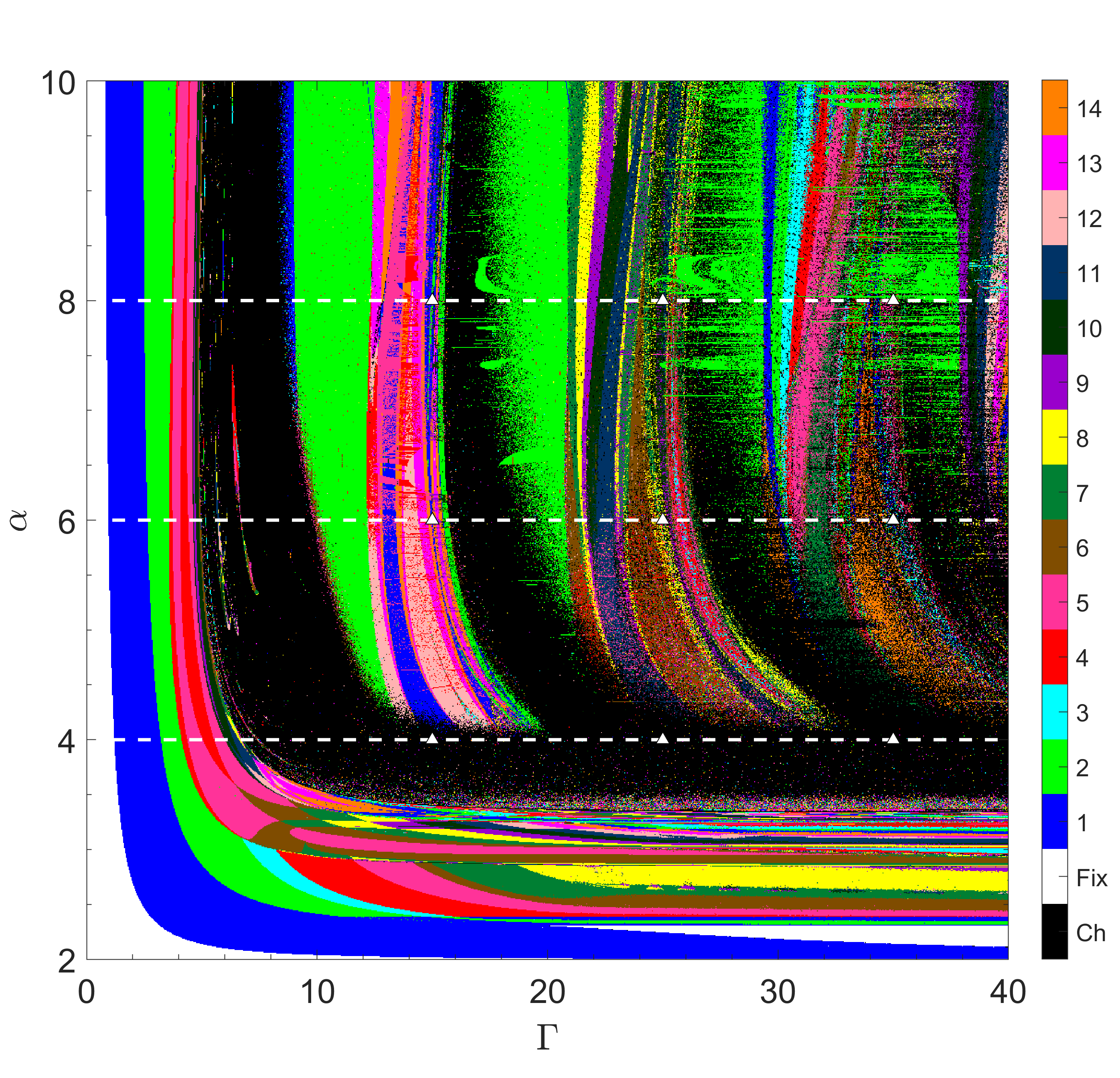
Figure 4: Isospike diagram obtained changing control parameters $\alpha$ and $\Gamma$. 1000x1000 parameter points are displayed. The number of peaks in a period is represented in colors according to the color bar shown in the right. Colors were recycled after 14 to represent more peaks per period. The initial conditions correspond to a constant value $x_{in}(t)=1$ $\forall t\in(-\Gamma,0)$ for each point of the diagram. To count the number of peaks a time of $200\Gamma$ was recorded after a transient time of $1000\Gamma$. Horizontal dashed lines correspond to the bifurcation diagrams of Fig. 2.

A more general picture of the global behavior can be obtained plotting isospike diagrams in which a color scale indicates the number of peaks in a given period of the variable or black in the case of chaotic solutions freire2011stern ; freire2013antiperiodic . Figure 4 shows an isospike diagram as parameters $\alpha$ and $\Gamma$ were varied. As shown in this figure intricate patterns arise in the parameter space, even in regions of high delay $\Gamma$ where chaos is to be expected. Several regions of periodicity are shown matching those seen in Fig. 2 reveling the complexity of the model as $\alpha$ and $\Gamma$ grow. The temporal series presented in Fig. 1 are also coherent whit these figures revealing that a region consists of similar series with variations due to creation and destruction of peaks while different regions will have different series structures. This patterns are examples of the intricacy and richness of delayed systems.

4 Impact of the multistability

The multistability in this system is ubiquitous in large regions of the parameter space. To gain insight, we consider four initial condition functions in the interval $(-\Gamma,0)$: a non-null constant value, a linear function, and two other periodic functions amil2015organization combining sinusoidal functions:

$$x_{A}(t)=1$$ (4)

$$x_{B}(t)=0.7\frac{t}{\Gamma}+0.3$$ (5)

$$x_{C}(t)=\frac{1}{4}\sin\Bigg{(}\frac{7\pi t}{\Gamma}+\phi\Bigg{)}\sin\Bigg{(}\frac{7\pi t}{2\Gamma}+\frac{\phi}{2}\Bigg{)}+x_{\mathrm{off}}$$ (6)

$$x_{D}(t)=\frac{1}{40}\sin\bigg{(}\frac{7\pi t}{\Gamma}+\phi\bigg{)}\bigg{[}\sin\bigg{(}\frac{7\pi t}{2\Gamma}+\frac{\phi}{2}\bigg{)}+4\bigg{]}+x_{\mathrm{off}}.$$ (7)

Using these functions we characterize systematically the abundance of coexisting solutions.

To illustrate the multistability, firstly, we selected two points labelled 1 ($\Gamma_{1}=18$, $\alpha_{1}=4$) and 2 ($\Gamma_{2}=20$, $\alpha_{2}=4$) and three different initial condition functions. These functions were labelled a, b, ch, obtained changing the parameters $\phi$ and $x_{\mathrm{off}}$ of Eq. (6). In Fig. 5 we show six temporal series (left column) and the respective recurrence plots (right column) corresponding to the two mentioned points and the three initial conditions. Both representation, temporal series and recurrence plot, provide supplementary pictures of the dynamics. In all the cases, the solutions labeled a and b are periodic while the corresponding to ch are chaotic. The characteristics of the periodic solutions at each point depend on the initial conditions, for example, in a1 we observe a period of 27.3 and 4 peaks per period while in a2 the period is 54.5 and there are 10 peaks per period. Nevertheless, when comparing panels a and b for both points, 1 and 2, the period and the number of peaks is multiplied by 3 suggesting a similar bifurcation scenario.

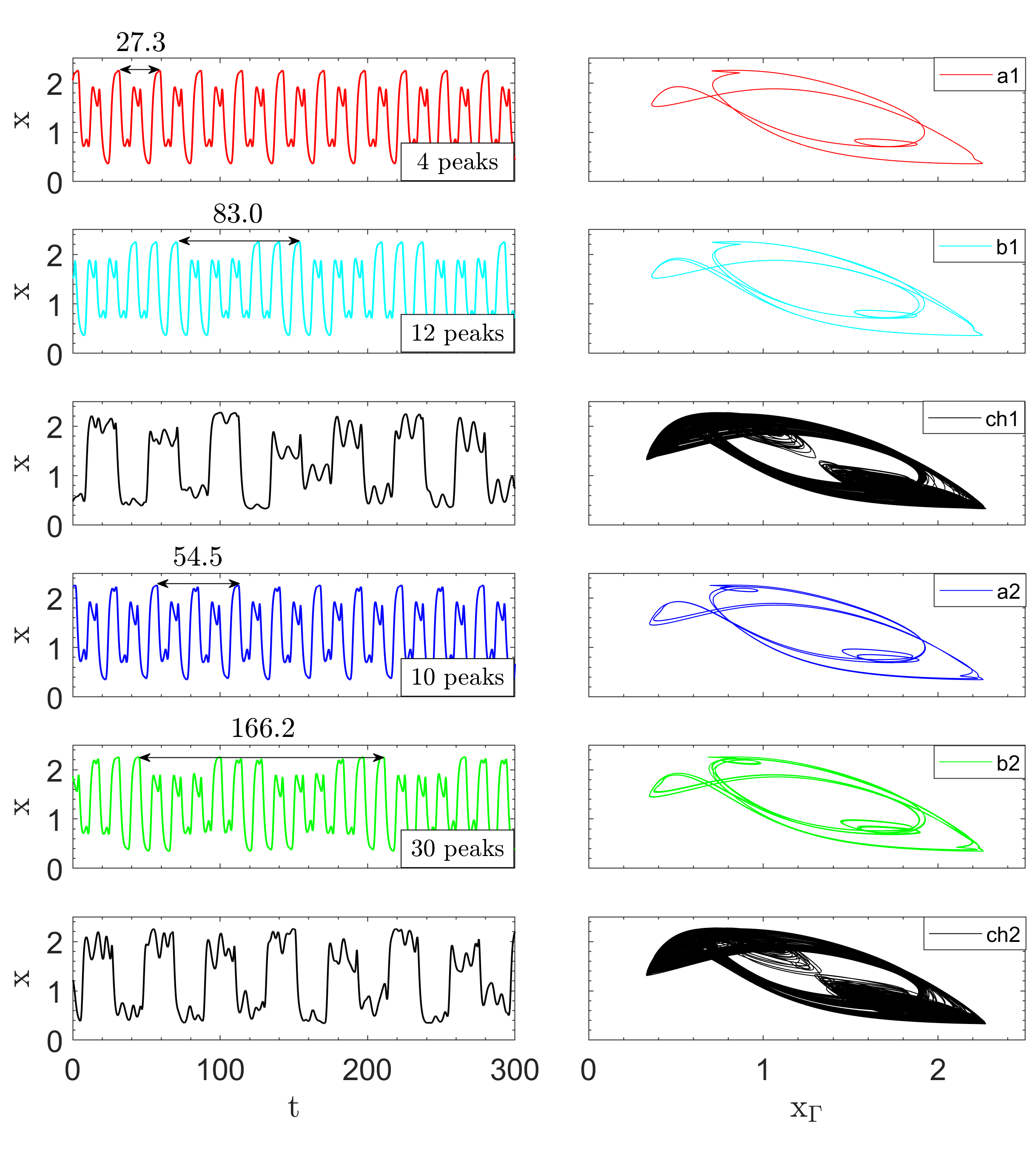
Figure 5: Coexisting solutions for different initial conditions in two fixed points of the parameter space. The temporal series and recurrence plot a1, b1 and ch1 correspond to the point $\Gamma=18$, $\alpha=4$ and a2, b2 and ch2 correspond to $\Gamma=20$, $\alpha=4$. The initial condition function is given by Eq. (6) with control parameters $\phi=0$ and $x_{\mathrm{off}}=0.35$ for a1 and a2, $\phi=\pi$ and $x_{\mathrm{off}}=0.3$ for b1 and b2 and $\phi=\pi$ and $x_{\mathrm{off}}=0.4$ for ch1 and ch2. A transient time of $2000\Gamma$ was neglected.

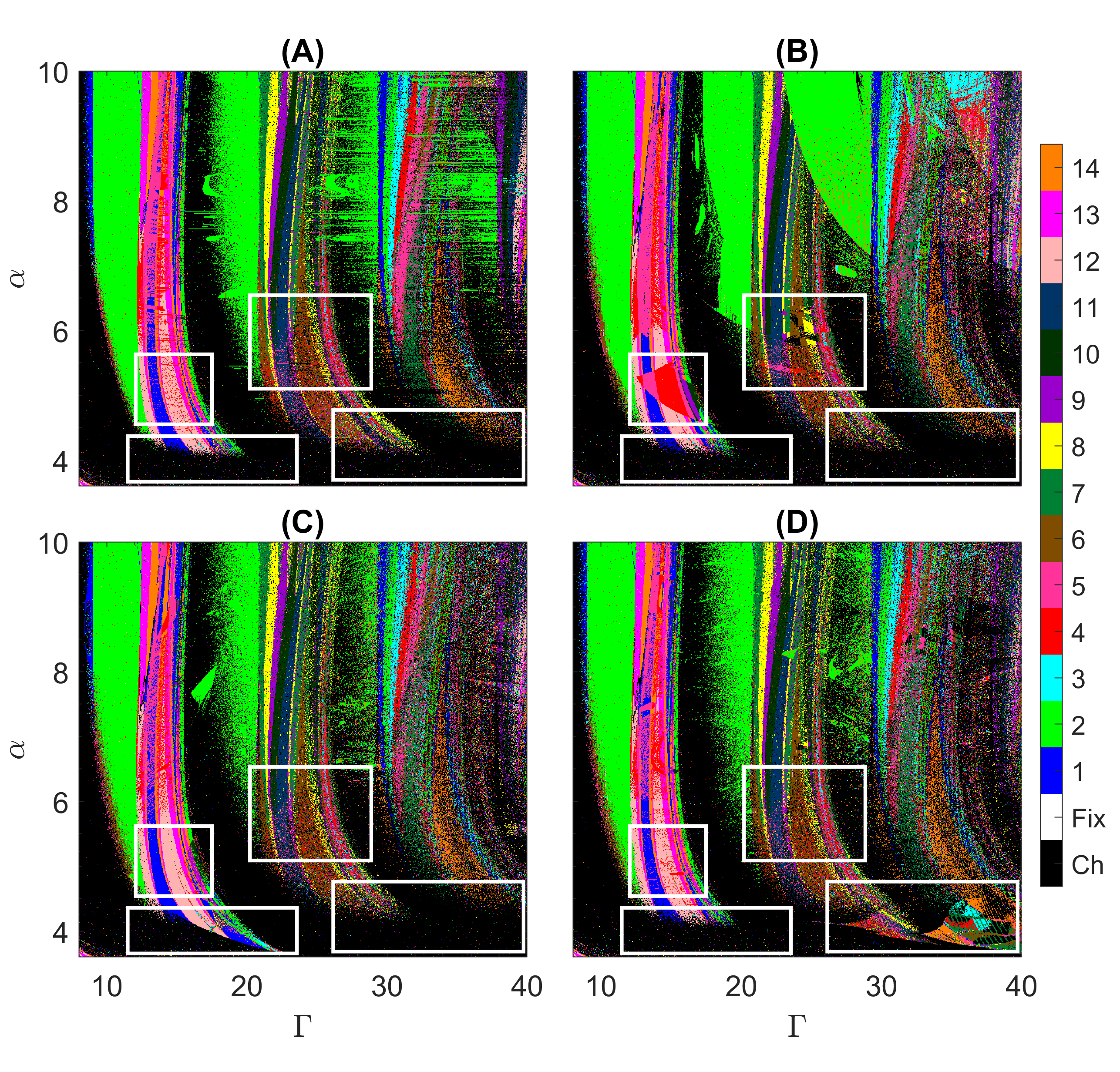
Figure 6: Isospike diagrams for different initial conditions functions. Each diagram displays 1000x1000 parameter points. The number of peaks in a period is represented in color. Colors were recycled after 14 to represent more peaks per period. The initial conditions are shown in Eq. (4) for (A), Eq. (5) for (B), Eq. (6) with $\phi=0$ and $x_{\mathrm{off}}=0.3$ for (C) and Eq. (7) with $\phi=0$ and $x_{\mathrm{off}}=0.33$ for (D). To count the number of peaks a time of $200\Gamma$ was recorded after a transient time of $1000\Gamma$.

Figure 6 shows isospike diagrams corresponding to the four initial condition functions, Eqs. 4-7, in a large region of the parameter space. Each point in these diagrams was obtained starting with the same initial conditions function. In all the panels we appreciate chaotic or periodic regions intermingled. Nevertheless, we observe that although some regions are similar in all the panels there are others that differs notably. To identify the regions which present more variations we included white boxes in Fig. 6. These variations demonstrate that multistability is not evenly distributed in the parameter space. In particular, for sufficiently low values of $\alpha$ or $\Gamma$, it appear only one stable solution while increasing one or both parameters leads in the majority of the cases to multistable behavior.

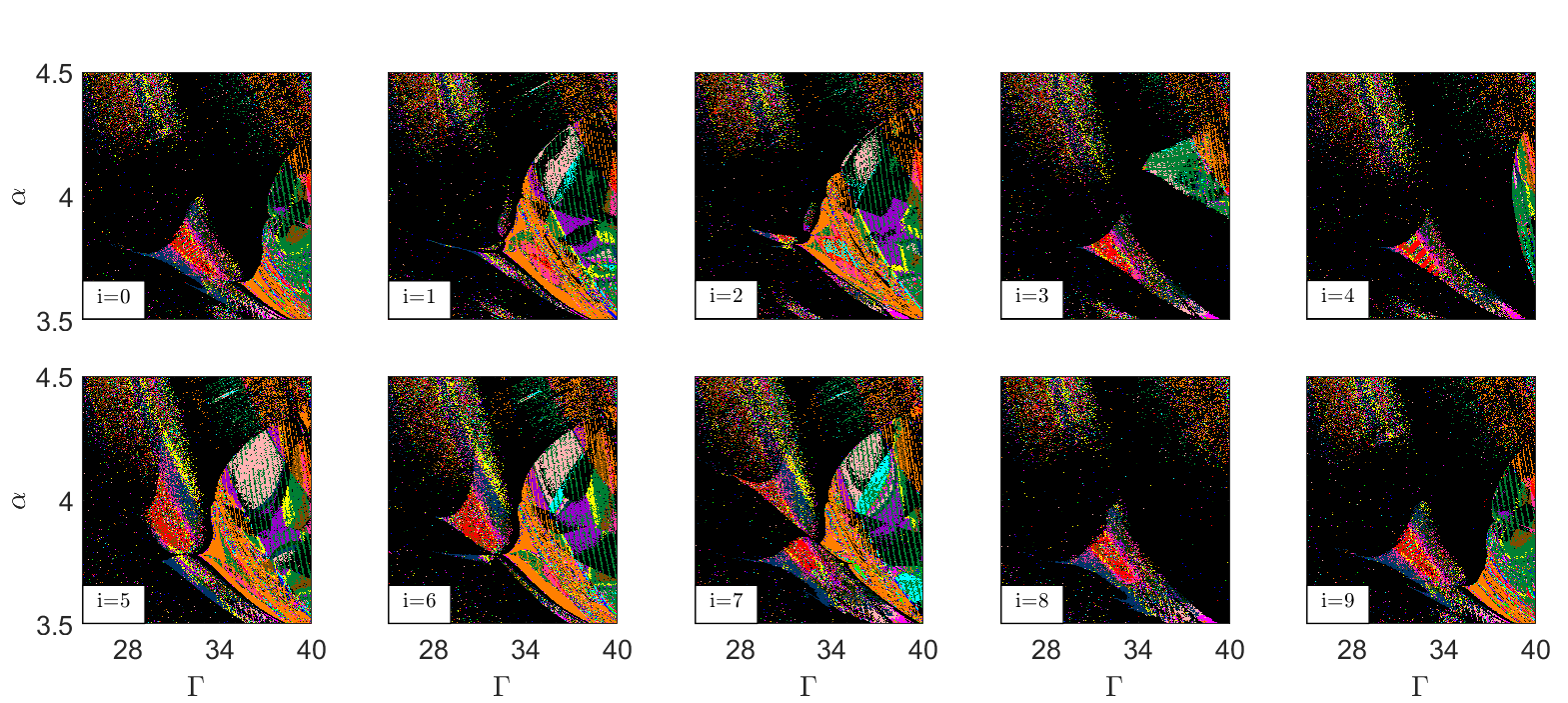
Figure 7: Parameter space diagrams for a family of initial conditions. The initial conditions were set to Eq. (7) with $x_{\mathrm{off}}=0.35$ and $\phi=\frac{4\pi i}{10}$ with $i=0,1,...\,9$. Each diagram displays 500x500 parameter points. To count the number of peaks, a time of $200\Gamma$ was recorded after a transient time of $2000\Gamma$.

To further quantify multistability, we selected a family of functions, given by Eq. 7, and changed systematically the parameter values. Then, the solutions obtained were analyzed for different control parameter values. Figure 7 shows the changes in peaks count for a smaller region of the parameter space as the initial conditions are changed. The initial conditions for each diagram correspond to the Eq. (7) with $x_{\mathrm{off}}=0.35$ and $\phi=\frac{4\pi i}{10}$ for $i=0,1,...\,9$. Small variations between the diagrams indicate the coexistence of multiple solutions for different initial conditions, even when only the phase is changed. To further assess this observation, the right diagram of Fig. 8 shows the number of distinct solutions that appear in Fig. 7 for every point of the parameter space, revealing a region where no periodic solutions were observed (black) and regions where multiple solutions coexist for different initial conditions functions (color). The left diagram of Fig. 8 shows the same analysis for a different region of the parameter space and a the family of initial conditions functions given by (6) with $x_{\mathrm{off}}=0.35$ and $\phi=\frac{4\pi i}{10}$ for $i=0,1,...\,9$. For this condition, a region without multistability (white) clearly appears.

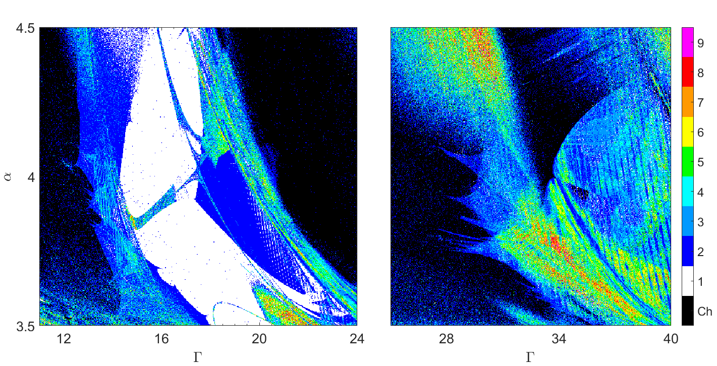
Figure 8: Number of distinct solutions as the initial conditions were varied for a region of the parameter space. The initial conditions were set to Eq. (6) for the left diagram and Eq. (7) for the right diagram with $x_{\mathrm{off}}=0.35$ and $\phi=\frac{4\pi i}{10}$ with $i=0,1,...\,9$ and the number of peaks was recorded for each diagram. The number of different solutions is represented in color for each point of the parameter space. Each diagram displays 500x500 parameter points. To count the number of peaks a time of $200\Gamma$ was recorded after a transient time of $2000\Gamma$.

A distinctive region of two solutions is shown in the left diagram of Fig. 8 for the 10 initial conditions functions selected. To continue with the study of multistability in this region two points $\Gamma=18$, $\alpha=4$ and $\Gamma=20$, $\alpha=4$ were selected and a map of coexisting solutions was made as the initial conditions vary inside the same family of functions. Figure 9 shows the different solutions that arise for the points $\Gamma=18$, $\alpha=4$ (left diagram) and $\Gamma=20$, $\alpha=4$ (right diagram), as initial conditions are changed. Initial conditions were set to Eq. (6) and parameters $\phi$ and $x_{\mathrm{off}}$ were varied finding two periodic solutions and a region of chaos for both points. Time series are shown in Fig 5. Similar patterns are observed between both diagrams, primarily the fact that regions of a1 in the left diagram correspond to regions of a2 in the right diagram and some structure remains on the frontier with the chaotic solutions.

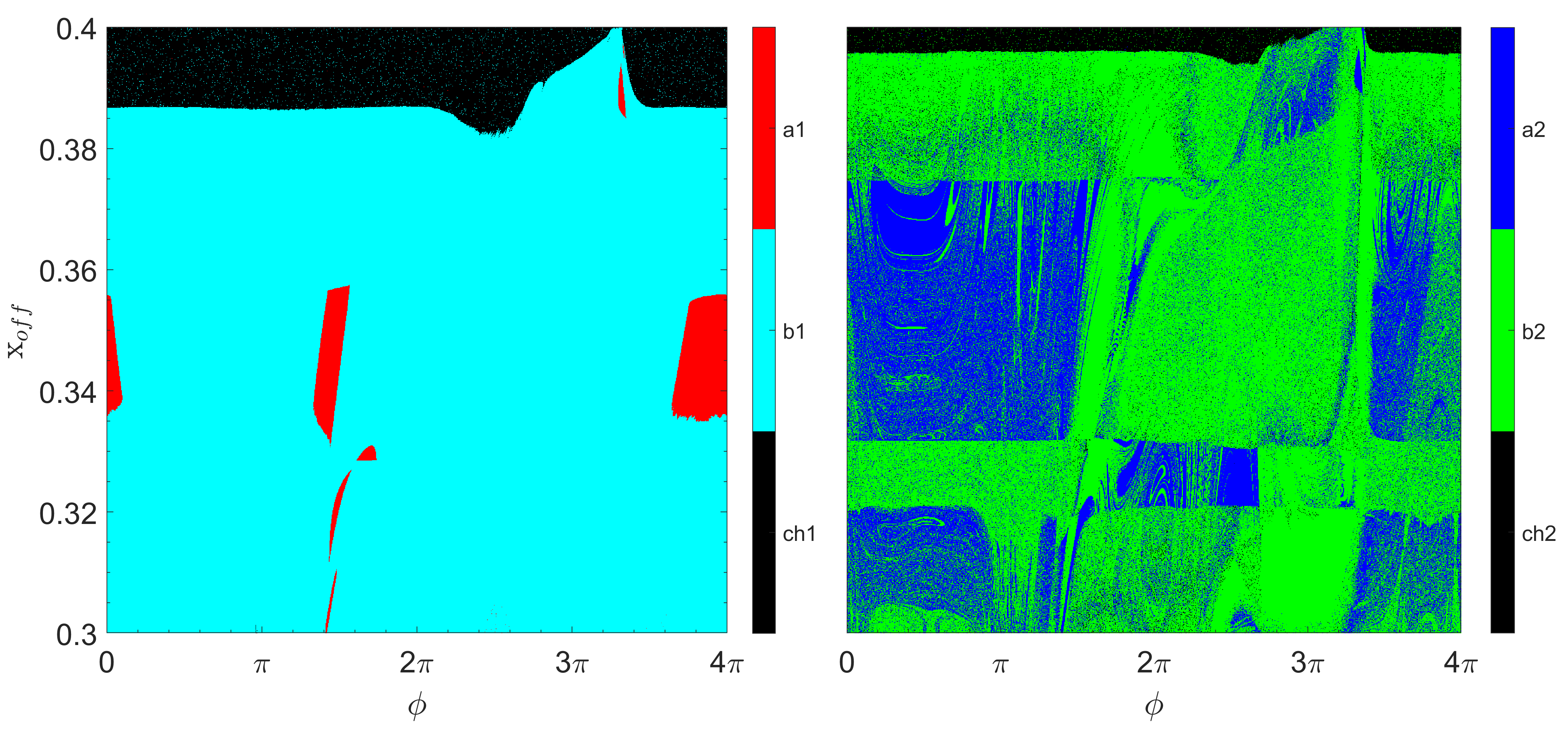
Figure 9: Map of coexisting solutions in a fixed point of the parameter space as the initial conditions are changed. Each diagram displays 1000x1000 parameter points. The left diagram corresponds to the point $\alpha=4$, $\Gamma=18$ and the diagram to the right to the point $\alpha=4$, $\Gamma=20$. The initial conditions were set to Eq. (6) as parameters $\phi$ and $x_{\mathrm{off}}$ were varied. A transient time of $2000\Gamma$ was neglected.

5 Conclusion

The Mackey-Glass delayed model was studied in this work using a previously validated numerical scheme. By means of temporal series, bifurcation and isospike diagrams we explored the parameter space expressed in terms of the dimensionless production rate and decay. In general terms, the complexity increases as increasing the delay. The presence of tongues of stability in the isospike diagrams is characteristics of this system.

Varying the initial condition function we found the coexistence of several solutions, i.e. multistability, in a broad range of values of space parameters. Moreover, periodic solutions consisting of maximums of several amplitudes but in different order are abundant in various of these regions. We characterized the coexisting solutions, either periodic or chaotic, in the parameter space. Selecting representative families of initial condition function we quantitatively evaluated the impact of the multistability. We also showed the existence of hysteresis loops by sweeping up and down the delay parameter in the bifurcation diagrams. Undoubtedly, the range of possible applications of delayed systems will continue to enlarge in the near future.

References

- [1] Michael C Mackey and Leon Glass. Oscillation and chaos in physiological control systems. Science, 197(4300):287–289, 1977.
- [2] Jacques Bélair. Dynamical Disease: Mathematical Analysis of Human Illness;[the Papers are Based on a NATO Advanced Research Workshop Held in Mont Tremblant, Québec, Canada in February 1994]. AIP Press, 1995.
- [3] Debabrata Biswas and Tanmoy Banerjee. Time-Delayed Chaotic Dynamical Systems. Springer, 2018.
- [4] Jack K Hale and Sjoerd M Verduyn Lunel. Introduction to functional differential equations, volume 99. Springer Science & Business Media, 2013.
- [5] Leandro Junges and Jason AC Gallas. Intricate routes to chaos in the mackey–glass delayed feedback system. Physics Letters A, 376(18):2109––2116, 2012.
- [6] Jerome Losson, Michael C Mackey, and Andre Longtin. Solution multistability in first-order nonlinear differential delay equations. Chaos: An Interdisciplinary Journal of Nonlinear Science, 3(2):167–176, 1993.
- [7] Boualem Mensour and André Longtin. Controlling chaos to store information in delay-differential equations. Physics Letters A, 205(1):18–24, 1995.
- [8] Tong Kun Lim, Keumcheol Kwak, and Mijeong Yun. An experimental study of storing information in a controlled chaotic system with time-delayed feedback. Physics Letters A, 240(6):287–294, 1998.
- [9] Brian B Zhou and Rajarshi Roy. Isochronal synchrony and bidirectional communication with delay-coupled nonlinear oscillators. Physical Review E, 75(2):026205, 2007.
- [10] Kestutis Pyragas. Synchronization of coupled time-delay systems: Analytical estimations. Physical Review E, 58(3):3067, 1998.
- [11] Min-Young Kim, Christopher Sramek, Atsushi Uchida, and Rajarshi Roy. Synchronization of unidirectionally coupled mackey-glass analog circuits with frequency bandwidth limitations. Physical Review E, 74(1):016211, 2006.
- [12] EM Shahverdiev, RA Nuriev, RH Hashimov, and KA Shore. Chaos synchronization between the mackey–glass systems with multiple time delays. Chaos, Solitons & Fractals, 29(4):854–861, 2006.
- [13] A Namajūnas, K Pyragas, and A Tamaševičius. An electronic analog of the mackey-glass system. Physics Letters A, 201(1):42–46, 1995.
- [14] Pablo Amil, Cecilia Cabeza, and Arturo C Marti. Exact discrete-time implementation of the mackey–glass delayed model. IEEE Transactions on Circuits and Systems II: Express Briefs, 62(7):681–685, 2015.
- [15] Pablo Amil, Cecilia Cabeza, Cristina Masoller, and Arturo C Martí. Organization and identification of solutions in the time-delayed mackey-glass model. Chaos: An Interdisciplinary Journal of Nonlinear Science, 25(4):043112, 2015.
- [16] Hal L Smith. An introduction to delay differential equations with applications to the life sciences, volume 57. Springer New York, 2011.
- [17] Alfredo Bellen and Marino Zennaro. Numerical methods for delay differential equations. Oxford university press, 2013.
- [18] Joana G Freire and Jason AC Gallas. Stern–brocot trees in cascades of mixed-mode oscillations and canards in the extended bonhoeffer–van der pol and the fitzhugh–nagumo models of excitable systems. Physics Letters A, 375(7):1097–1103, 2011.
- [19] Joana G Freire, Cecilia Cabeza, Arturo Marti, Thorsten Pöschel, and Jason AC Gallas. Antiperiodic oscillations. Scientific Reports, 3, 2013.