Boosting Salient Object Detection with Transformer-based Asymmetric Bilateral U-Net

Abstract

Existing salient object detection (SOD) methods mainly rely on U-shaped convolution neural networks (CNNs) with skip connections to combine the global contexts and local spatial details that are crucial for locating salient objects and refining object details, respectively. Despite great successes, the ability of CNNs in learning global contexts is limited. Recently, the vision transformer has achieved revolutionary progress in computer vision owing to its powerful modeling of global dependencies. However, directly applying the transformer to SOD is suboptimal because the transformer lacks the ability to learn local spatial representations. To this end, this paper explores the combination of transformers and CNNs to learn both global and local representations for SOD. We propose a transformer-based Asymmetric Bilateral U-Net (ABiU-Net). The asymmetric bilateral encoder has a transformer path and a lightweight CNN path, where the two paths communicate at each encoder stage to learn complementary global contexts and local spatial details, respectively. The asymmetric bilateral decoder also consists of two paths to process features from the transformer and CNN encoder paths, with communication at each decoder stage for decoding coarse salient object locations and fine-grained object details, respectively. Such communication between the two encoder/decoder paths enables AbiU-Net to learn complementary global and local representations, taking advantage of the natural merits of transformers and CNNs, respectively. Hence, ABiU-Net provides a new perspective for transformer-based SOD. Extensive experiments demonstrate that ABiU-Net performs favorably against previous state-of-the-art SOD methods. The code is available at https://github.com/yuqiuyuqiu/ABiU-Net.

I Introduction

Salient object detection (SOD) aims at detecting the most visually conspicuous objects or regions in an image [1, 2, 3, 4, 5, 6, 7, 8, 9]. It has a wide range of computer vision applications such as human-robot interaction [10], content-aware image editing [11], image retrieval [12], object recognition [13], image thumbnailing [14], weakly supervised learning [15], etc. In the last decade, convolutional neural networks (CNNs) have significantly pushed forward this field. Intuitively, the global contextual information (existing in the top CNN layers) is essential for locating salient objects, while the local fine-grained information (existing in the bottom CNN layers) is helpful in refining object details [1, 16, 17, 18, 19, 8, 9]. This is why the U-shaped encoder-decoder CNNs have dominated this field [20, 21, 22, 23, 24, 25, 16, 26, 17, 27, 28, 3, 29, 30, 31, 32, 33, 2, 34, 35, 36], where the encoder extracts multi-level deep features from raw images and the decoder integrates the extracted features with skip connections to make image-to-image predictions [20, 21, 22, 23, 24, 25, 16, 26, 17, 27, 28, 3, 29, 37]. The encoder is usually the existing CNN backbones, e.g., ResNet [38], while most efforts are put into the design of the decoder [30, 31, 32, 35, 33]. Although remarkable progress has been seen in this direction, CNN-based encoders share the intrinsic limitation of extracting features from images in a local manner. The lack of powerful global modeling has been the main bottleneck for CNN-based SOD.

To this end, we note that recent popular transformer networks [39, 40] provide a new perspective on this problem. Originating from machine translation [39], transformers entirely reply on self-attention to model global dependencies of sequence data directly. Viewing image patches as tokens (words) in natural language processing (NLP) applications [40], transformers can be applied to learn powerful global feature representations for images.

Since the global relationship modeling of transformers is beneficial to SOD for locating salient objects in a natural scene, some works have tried to bring transformers into SOD [41, 42]. However, we note that existing transformer-based SOD methods [41, 42] entirely rely on the transformer to extract global features by using the transformer as the encoder. They ignore the effect of local representations, which is also essential for SOD in refining object details [24, 25, 16, 26, 17, 27, 28, 3, 29, 30, 31, 32, 33, 35, 19, 8], as mentioned above. Therefore, existing SOD methods have gone from one extreme to the other, i.e., from the lack of powerful global modeling (CNN-based methods) to the lack of local representation learning (transformer-based methods).

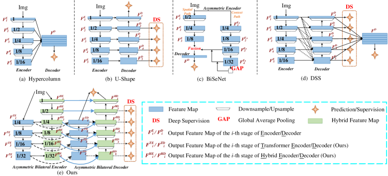
Figure 1: Illustration of various encoder-decoder architectures. (a) $\sim$ (e) indicate the architectures of Hypercolumn [43, 23, 26, 44, 45, 46, 42], U-shape [47, 32, 35, 48, 49, 33, 50, 51, 52, 53, 41], BiSeNet [54], DSS [55, 56] and our ABiU-Net, respectively. Note that the feature maps in (a) $\sim$ (d) (i.e., the blue rectangle) are not limited to transformer- or CNN-based feature maps.

Based on the above observation, how to achieve effective local representations in accompany with transformer networks would be the key to further boost SOD. To this end, we consider combining the merits of transformers and CNNs, which are adept at global relationship modeling and local representation learning, respectively. In this paper, we propose a new encoder-decoder architecture, namely Asymmetric Bilateral U-Net (ABiU-Net). Its encoder consists of two parts: Transformer Encoder Path (TEncPath) and Hybrid Encoder Path (HEncPath). TEncPath directly uses a transformer network for global relationship modeling, in order to locate salient objects. Since the transformer entirely relies on self-attention to extract global contextual features, TEncPath lacks local find-grained features that are essential for refining object details/boundaries. Hence, we introduce HEncPath by stacking several convolution stages, to enhance the locality of the encoder. To fuse the global and local features, the inputs of each stage of HEncPath are from the preceding convolution stage as well as the corresponding TEncPath stage, respectively. In this way, HEncPath introduces locality into feature representations with the guide of global contexts from TEncPath. Therefore, HEncPath is a hybrid encoding of global long-range dependencies and local representations. Note that HEncPath is lightweight with a small number of channels and a fast downsampling strategy.

In the phase of decoding, we design an asymmetric bilateral decoder containing two simple paths, namely Transformer Decoder Path (TDecPath) and Hybrid Decoder Path (HDecPath), which are utilized to decode feature representations from TEncPath and HEncPath, respectively. TDecPath decodes coarse salient object locations, while HDecPath is expected to further refine object details/boundaries. We adopt the standard channel attention mechanism to enhance the feature representations from TEncPath and HEncPath. The output of TDecPath at each stage is fed into the corresponding stage of HDecPath so that these two decoder paths can communicate and learn complementary information, i.e., coarse locations and find-grained details, respectively.

Generally, ABiU-Net is an extension of the U-shaped architecture, and it mainly aims to explore a balanced combination of transformers and CNNs to address the challenge of accurately segmenting salient object in natural scenes. Although transformer-based U-Net models have been explored, they usually replace the encoder/decoder of classic U-Net with transformers or the simple serial combination of CNNs and transformers [57, 58]. In contrast, this paper introduces a bilateral encoder-decoder structure and enables the communication between the two paths, which is ignored by previous studies. Besides, the existing multi-column architectures [54, 59] are usually built in a separate way, i.e., only the output features of the various paths are fused. This late fusion manner can not fully utilize the complementary advantages of different paths. Compared to their late fusion manner, the multi-level communication of ABiU-Net has the following advantage: the global features learned from the transformer path can guide the learning of detailed features of the CNN path, and in turn, the detailed features can promote the optimization of global features. In brief, we can conclude our contribution and novelty as: we propose a new network architecture, ABiU-Net, to make complementary use of global contextual features (for locating salient objects) and local detailed representations (for refining object details) by exploring the deep cooperation between transformers and CNNs. Extensive experiments demonstrate the remarkable superiority of ABiU-Net. Considering that ABiU-Net is an elegant architecture without carefully designed modules or engineering skills, ABiU-Net provides a new perspective for SOD in the transformer era.

II Related Work

II-A CNN-based Salient Object Detection

In the last decade, the accuracy of SOD has been remarkably boosted due to the multi-level representation capability of CNNs [24, 25, 16, 26, 17, 27, 28, 3, 29, 30, 31, 32, 33, 4, 35]. It is widely accepted that the high-level semantic information extracted by the top CNN layers is beneficial to locating the coarse positions of salient objects, while the low-level information extracted by the bottom layers can refine the object details. Hence, both the high-level and low-level information are important for accurate SOD [60, 23, 16, 25, 24, 26, 17, 61, 56, 37]. Most existing CNN-based SOD methods use pre-trained image classification models, e.g., ResNet [38], as encoders and focus on designing effective decoders by aggregating multi-level features [56, 45, 30, 62, 48, 35, 37]. For example, Wu et al. [63] introduced an extremely-downsampled network to show the importance of high-level features for SOD. Li et al. [6] built dense attention upon multi-level features simultaneously for feature selection in SOD. Mei et al. [9] aimed at capturing dense multi-scale contexts to enhance the feature discriminability. Zhang et al. [8] proposed a novel trifurcated cascaded refinement network to explore multi-level feature fusion and global information representation for SOD. In addition, Liu et al. [3, 29] also designed new encoders for lightweight SOD.

However, CNNs are limited in global dependency modeling which is essential for locating salient objects, as noted in Section I. To alleviate this issue, some modules are introduced to learn the long-distance dependency information. For example, Hu et al. [18] designed a spatial attenuation context module to maximize the integration of local and global image context within, around, and beyond the salient objects. Gu et al. [64] introduced a pyramid constrained self-attention operation to capture objects at various scales. Qiu et al. [65] designed attentive atrous spatial pyramid pooling (A2SPP) by adding a new cubic information-embedding attention module at each branch of atrous spatial pyramid pooling (ASPP) [66] to encode multi-level dependency information for SOD. A comprehensive review of CNN-based SOD is beyond the scope of this paper, and we recommend referring to [67] for a more thorough analysis.

Due to the local receptive fields of convolution operations, the ability of the above CNN-based models in learning global semantic information is limited, which is the main bottleneck for improving CNN-based SOD. To solve this problem, we note that recent vision transformers [39, 40] are adept at global relationship modeling. Thus, we attempt to explore vision transformers for boosting SOD and delve into the effective cooperation of transformers and CNNs in learning both global contexts and local features.

II-B Transformer-based Salient Object Detection

The transformer is first proposed in NLP for machine translation [39]. The transformer network alternately stacks multi-head self-attention modules, aiming at estimating the global dependencies between every two patches, and a multilayer perceptron, aiming at feature enhancement. Recently, researchers have brought the transformer into computer vision and achieved remarkable achievements. Specifically, Dosovitskiy et al. [40] made the first attempt to apply the transformer to image classification, attaining competitive performance on the ImageNet dataset [68]. They split an image into a sequence of flattened patches that are fed into transformers. Following [40], lots of studies have emerged in a short period, and much better performance than state-of-the-art CNNs has been achieved [69, 70, 71, 72, 73]. For example, Cui [74] first proposed a dynamic aggregation module to adaptively select the frames for feature enhancement, which improved the inference speed of feature aggregation-based video object detectors. Then, to get better performance, Cui [75] focused on transformer-based video object detection and introduced a query aggregation module to improve the quality of queries by aggregating queries according to the features of input frames.

For SOD, Mao et al. [42] adopted Swin Transformer [71] as the encoder and designed a simple CNN-based decoder to predict saliency maps recently. However, compared to CNN-based salient object detection models, they only replaced the CNN-based encoder with the transformer-based encoder. To further explore the superiority of vision transformers in SOD, Liu et al. [41] introduced a novel pure transformer model for SOD, bringing a great success. They designed a new token upsampling strategy and fused multi-level patch tokens to make transformer more suitable for SOD. Moreover, Mao et al. [76] claimed that, compared to the CNN-based models, the superior performance of transformer-based models came from the effective global context modeling abilities. Although existing transformer-based works [18, 42, 41] solve the lack of global contexts in CNN-based SOD, they ignore the local representations that are essential for refining salient object details. In this paper, we work on how to effectively learn both global contexts and local features by exploring the cooperation of transformers and CNNs, so salient objects can be precisely located and segmented.

The proposed ABiU-Net uses the PVT [70], for global relationship modeling. In detail, PVT aims to introduce the pyramid structure into the transformer framework, which can generate multi-scale feature maps for dense prediction. PVT has four stages, each of which is comprised of a patch embedding layer and a $L_{i}$-layer transformer encoder. To obtain a pyramid structure, PVT uses a progressive shrinking strategy to control the scale of feature maps by patch embedding layers. In this way, PVT can generate feature maps of four different scales, i.e., 4-. 8-, 16-, and 32-stride with respect to the input image. PVT has a series of versions with different scales, namely PVT-Tiny, PVT-Small, PVT-Medium, and PVT-Large, whose numbers of parameters are similar to ResNet18, ResNet50, ResNet101, and ResNet152 [38], respectively. By default, the TEncPath of ABiU-Net uses PVT-Small.

II-C Encoder-decoder Architectures

This paper mainly designs a new encoder-decoder architecture, i.e., Asymmetric Bilateral U-Net (ABiU-Net), for SOD. To illustrate the novelty of ABiU-Net, we summarize various widely-used encoder-decoder architectures (not only for SOD) in Fig. 1. Hypercolumn [43] simply aggregates features from different levels of the encoder for final predictions, as shown in Fig. 1(a). The aggregated hyper-features are so-called Hypercolumns. The typical applications of the Hypercolumn encoder-decoder architecture in SOD include [23, 26, 44, 45, 46, 42]. As shown in Fig. 1(b), the U-shaped encoder-decoder architecture is the most widely-used. The main idea of U-shaped encoder-decoder is to supplement a contracting encoder with a symmetric decoder, where the pooling operations in the encoder are replaced with upsampling operations in the decoder. Deep supervision [77] is also imposed to ease the training process. Most SOD methods are based on or improve upon the U-shaped encoder-decoder architecture [24, 25, 16, 26, 61, 17, 27, 28, 30, 32, 48, 49, 33, 50, 51, 52, 53, 31, 5, 3, 29, 2, 41, 35]. As shown in Fig. 1(c), BiSeNet [54], designed for semantic segmentation, has two encoder paths: (1) the spatial path that stacks only three convolution layers to obtain the $1/8$ feature map to retain affluent spatial details, and (2) the context path connects a global average pooling layer at the top. These two paths are fused for final prediction. Note that our “bilateral” is inspired by BiSeNet [54]. Hence, we discuss the difference between the proposed model and BiSeNet here. On one hand, although both BiSeNet and ABiU-Net have a two-path encoder, ABiU-Net enables interaction between the two paths, while BiSeNet does not. On the other hand, ABiU-Net supplements an asymmetric bilateral decoder for better fusing the information from the two-path encoder, while BiSeNet directly utilizes the features of the encoder for final prediction. Another widely-used encoder-decoder architecture is Holistically-nested Edge Detector (HED) [55]. Hou et al. [56] designed a new HED-based saliency detection model, namely DSS, by introducing short connections to the skip-layer structure within the HED, which is shown in Fig. 1(d). From Fig. 1, we can clearly see the difference between the proposed ABiU-Net and other architectures. Therefore, we can conclude that ABiU-Net is a new encoder-decoder architecture in the transformer era.

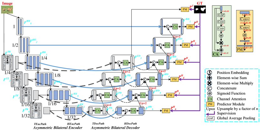
Figure 2: Framework of the proposed Asymmetric Bilateral U-Net (ABiU-Net).

III Methodology

This section presents the proposed ABiU-Net for accurate SOD. We first describe the overall framework of ABiU-Net in Section III-A. Then, we introduce the asymmetric bilateral encoder and the asymmetric bilateral decoder in Section III-B and Section III-C, respectively.

III-A Overall Framework

Since previous CNN-based SOD methods [20, 21, 22, 23, 24, 25, 16, 26, 17, 27, 28, 3, 29, 19] lack powerful global context modeling and existing transformer-based SOD methods [42, 41] lack effective local representations, in this paper, we aim at learning both global contexts and local features for locating salient objects and refining object details, respectively. For this goal, we improve the traditional U-Net [47] to the new ABiU-Net by exploring the cooperation of transformers and CNNs, so ABiU-Net can inherit their merits for global context modeling and local feature learning, respectively. ABiU-Net consists of an asymmetric bilateral encoder and an asymmetric bilateral decoder.

As shown in Fig. 2, the asymmetric bilateral encoder of ABiU-Net contains two parts: TEncPath in grey and HEncPath in blue. TEncPath is one well-known transformer network, e.g., PVT [70], with four stages. The main issue is that the transformer network only focuses on learning long-range dependencies with the sacrifice of local information. This is remedied by another encoder path, i.e., HEncPath. HEncPath stacks six lightweight convolution stages. In particular, the inputs of the $3^{\rm rd}$ $\sim$ $6^{\rm th}$ stages are not only from the preceding stage but also from the corresponding transformer stage that has the same output stride. Hence, HEncPath can achieve the hybrid encoding of global long-range dependencies and local representations.

The asymmetric bilateral decoder also consists of two paths, namely TDecPath and HDecPath, decoding feature representations from TEncPath and HEncPath, respectively. TDecPath has four stages, which can be viewed as a simple top-down generation path to regress the coarse locations of salient objects. HDecPath is a hybrid decoding process with six stages in the top-down view. The input of HDecPath at each stage is not only from HEncPath but also from TDecPath. In this way, two decoder paths can communicate and learn complementary information, i.e., the coarse locations of salient objects decoded in TDecPath would guide the learning of HDecPath to further refine object details. We will introduce the decoder in Section III-C.

The output feature map of HDecPath at the last stage is used for the final saliency map prediction. We also impose deep supervision [77] on the other five stages of HDecPath and the last stage of TDecPath. To achieve this, we design a simple Prediction Module (PM), which converts a feature map to a saliency map. PM first adopts two successive $3\times 3$ convolution layers with batch normalization and nonlinearization to convert the input feature map to a single-channel map. Then, the sigmoid activation function is followed to predict the saliency probability map, whose values range from 0 to 1. The proposed ABiU-Net is trained end-to-end using the standard binary cross-entropy loss (BCE). Suppose the saliency maps of HDecPath are denoted by $\mathbf{P}^{H}_{i}$ ($i\in{1,2,3,4,5,6}$) from bottom to top, and the saliency map of TDecPath is denoted by $\mathbf{P}^{T}$. The total training loss can be calculated as

$$L=\mathcal{L}_{\rm BCE}(\mathbf{P}^{H}_{1},\mathbf{G})+\lambda\sum_{i=2}^{6}\mathcal{L}_{\rm BCE}(\mathbf{P}^{H}_{i},\mathbf{G})+\lambda\mathcal{L}_{\rm BCE}(\mathbf{P}^{T},\mathbf{G}),$$ (1)

where $\mathbf{G}$ represents the ground-truth saliency map. $\lambda$ is a weighting scalar for loss balance. In this paper, we empirically set $\lambda$ to 0.4, as suggested by [78, 2, 3, 29, 30, 31]. During testing, $\mathbf{P}^{H}_{1}$ is viewed as the final output saliency map.

III-B Asymmetric Bilateral Encoder

First of all, we want to clarify that the asymmetry of our bilateral encoder mainly refers to: i) two encoder paths are based on different networks (transformer and CNN); ii) the numbers of stages of these two paths are different (four for TEncPath and six for HEncPath); and iii) the targets that they are responsible for are different (global context modeling and hybrid feature encoding). Now, we describe how we designed it and the reasons behind it.

We use the popular transformer network, PVT [70], as TEncPath. All stages of PVT share a similar architecture, which consists of a patch embedding layer and several transformer blocks. Specifically, given an input image, PVT splits it into small patches with the size of $4\times 4$, using a patch embedding layer. Then, the flattened patches are added with a position embedding and fed into transformer blocks. From the second stage, PVT utilizes a patch embedding layer to shrink the feature map by a scale of 2 at the beginning of each stage, followed by the addition with a position embedding and then some transformer blocks. Suppose $\mathbf{F}^{\rm TE}_{1}$, $\mathbf{F}^{\rm TE}_{2}$, $\mathbf{F}^{\rm TE}_{3}$, and $\mathbf{F}^{\rm TE}_{4}$ denote the output feature maps of the four stages of PVT from bottom to top, and they have scales of $1/4$, $1/8$, $1/16$, and $1/32$ with 64, 128, 320, and 512 channels, respectively. Please refer to the original paper [70] for more details.

For HEncPath, we design a lightweight CNN-based sub-network to introduce the local sensitivity. Specifically, we stack six convolution stages whose outputs are $\mathbf{F}^{\rm HE}_{1}$, $\mathbf{F}^{\rm HE}_{2}$, $\mathbf{F}^{\rm HE}_{3}$, $\mathbf{F}^{\rm HE}_{4}$, $\mathbf{F}^{\rm HE}_{5}$, and $\mathbf{F}^{\rm HE}_{6}$ from bottom to top, respectively. Except for the last stage, a max-pooling layer with a stride of 2 is connected after each stage for feature downsampling, leading to output scales of $1$, $1/2$, $1/4$, $1/8$, $1/16$, and $1/32$ for six stages from bottom to top, respectively. The input image is fed into not only TEncPath but also HEncPath. The output of the first stage of HEncPath is used as the input of its second stage. From the third stage, the input of each stage is the concatenation of the feature map from the preceding stage and the feature map from the corresponding stage of TEncPath with the same resolution. The concatenated feature map is first connected to a $1\times 1$ convolution for integration. Then, HEncPath processes it through $N_{i}$ convolution layers with batch normalization and nonlinearization. Through using $\mathbf{F}^{\rm TE}_{i}$ as the input of HEncPath, it is easier for $\mathbf{F}^{\rm HE}_{i}$ to learn complementary local fine-grained features with the guidance of $\mathbf{F}^{\rm TE}_{i}$. Since TEncPath provides a high-level semantic abstraction for HEncPath, it is unnecessary to use a very deep or cumbersome CNN for HEncPath. Note that HEncPath also takes the original image as input so as to mine complementary local information from the image.

For a clear presentation, we can formulate these steps of HEncPath as

$$\mathbf{F}^{\rm HE}_{1} ={\rm Conv}^{3\times 3}_{\times N_{1}}(\mathbf{I}),$$ (2)

$$\mathbf{F}^{\rm HE}_{2} ={\rm Conv}^{3\times 3}_{\times N_{2}}({\rm MaxPool}(\mathbf{F}^{\rm HE}_{1})),$$

$$\mathbf{F}^{\rm HE}_{i} ={\rm Conv}^{3\times 3}_{\times N_{i}}({\rm Conv}^{1\times 1}({\rm MaxPool}(\mathbf{F}^{\rm HE}_{i-1})\ \copyright\ \mathbf{F}^{\rm TE}_{i-2})),$$

$$\qquad\qquad\qquad\text{for}\ i\in\{3,4,5,6\},$$

where $\mathbf{I}$ denotes the input color image. ${\rm Conv}^{1\times 1}(\cdot)$ is $1\times 1$ convolution. ${\rm Conv}^{3\times 3}_{\times N_{i}}(\cdot)$ represents $N_{i}$ successive $3\times 3$ convolutions with batch normalization and nonlinearization omitted for simplicity, where $N_{i}$ is the number of convolution layers at each stage of HEncPath. ${\rm MaxPool}(\cdot)$ is a max pooling layer with a stride of 2. “$\copyright$” represents the concatenation operation along the channel dimension. We set $N_{i}$ to 2 for $i\in\{1,2,3,4,5\}$, and we have $N_{6}=3$, with 16, 64, 64, 128, 256, and 256 output channels, respectively, to make HEncPath a lightweight sub-network.

With the asymmetric bilateral encoder, we obtain two sets of features with different characteristics. $\mathbf{F}^{\rm TE}_{i}$ ($i\in{1,2,3,4}$), generated by TEncPath, is based on global long-range dependence modeling, thus containing rich contextual information. On the other hand, $\mathbf{F}^{\rm HE}_{i}$ ($i\in{1,2,3,4,5,6}$) aims at learning complementary information to global modeling, guided by $\mathbf{F}^{\rm TE}_{i}$. Hence, $\mathbf{F}^{\rm HE}_{i}$ contains rich local features. The transformer features, $\mathbf{F}^{\rm TE}_{i}$, would be useful to locate salient objects with the global view on the image scenes, while the CNN features, $\mathbf{F}^{\rm HE}_{i}$, would be useful to refine object details with the local fine-grained representations. Therefore, the combination of the global features $\mathbf{F}^{\rm TE}_{i}$ and the local features $\mathbf{F}^{\rm HE}_{i}$ would lead to accurate SOD.

III-C Asymmetric Bilateral Decoder

Corresponding to the encoder, we design an asymmetric bilateral decoder containing two paths, i.e., TDecPath and HDecPath. TDecPath is utilized to decode feature representations from TEncPath, which can be viewed as a simple top-down generation path. The top stage takes $\mathbf{F}^{\rm TE}_{4}$ as input, and its output is denoted as $\mathbf{F}^{\rm TD}_{4}$. The $i$-th ($i\in\{3,2,1\}$) stage of TDecPath has two inputs, i.e., $\mathbf{F}^{\rm TE}_{i}$ from TEncPath and $\mathbf{F}^{\rm TD}_{i+1}$ from the preceding stage of TDecPath, generating the output $\mathbf{F}^{\rm TD}_{i}$. The main operations of TDecPath are as below. First of all, $\mathbf{F}^{\rm TE}_{4}$ $\sim$ $\mathbf{F}^{\rm TE}_{1}$ are separately fed into a $3\times 3$ convolution layer with batch normalization and nonlinearization to reduce the number of channels to (128, 64, 32, 16), generating feature maps $\hat{\mathbf{F}}^{\rm TE}_{i}$ ($i\in\{4,3,2,1\}$), respectively. This process can be formulated as

$$\hat{\mathbf{F}}^{\rm TE}_{i}={\rm Conv}^{3\times 3}(\mathbf{F}^{\rm TE}_{i}),\quad\text{for}\ i\in\{4,3,2,1\}.$$ (3)

After that, $\hat{\mathbf{F}}^{\rm TE}_{i}$ ($i\in\{3,2,1\}$) is concatenated with the output of the preceding stage in TDecPath. Note that $\hat{\mathbf{F}}^{\rm TE}_{4}$ is the only input of the fourth stage of TDecPath, so there is no concatenation operation. Then, we adopt the standard Channel Attention (CA) mechanism to process the concatenated feature map for feature enhancement. As shown in Fig. 2, the CA mechanism is a typical squeeze-excitation attention block [79] whose description is omitted here. After the CA block, we obtain $\mathbf{F}^{\rm TD}_{4}$, $\mathbf{F}^{\rm TD}_{3}$, $\mathbf{F}^{\rm TD}_{2}$, and $\mathbf{F}^{\rm TD}_{1}$ from top to bottom. Formally, this can be written as

$$\mathbf{F}^{\rm TD}_{4} ={\rm CA}(\hat{\mathbf{F}}^{\rm TE}_{4}),$$ (4)

$$\tilde{\mathbf{F}}^{\rm TD}_{i} ={\rm Conv}^{3\times 3}(\mathbf{F}^{\rm TD}_{i}),\quad\text{for}\ i\in\{4,3,2,1\},$$

$$\mathbf{F}^{\rm TD}_{i} ={\rm CA}(\hat{\mathbf{F}}^{\rm TE}_{i}\ \copyright\ {\rm Upsample}(\tilde{\mathbf{F}}^{\rm TD}_{i+1})),\quad\text{for}\ i\in\{3,2,1\},$$

where the $3\times 3$ convolution reduces the number of feature channels of $\mathbf{F}^{\rm TD}_{i}$ ($i\in\{4,3,2,1\}$) to the half. ${\rm Upsample}(\cdot)$ is to upsample the feature map by a factor of 2. In this way, TDecPath can decode the coarse locations of salient objects using the global contexts in TEncPath.

HDecPath is expected to further refine salient object details, guided by the coarse locations decoded by TDecPath. Hence, HDecPath takes two inputs: the features from TDecPath and HEncPath, providing the coarse locations of salient objects and the features about object details, respectively. HDecPath contains six decoder stages, whose outputs are denoted as $\mathbf{F}^{\rm HD}_{i}$ ($i\in\{1,2,3,4,5,6\}$). First, we connect the $3\times 3$ convolution layers (with batch normalization and nonlinearization) to the side-outputs of HEncPath and TDecPath, generating $\hat{\mathbf{F}}^{\rm HE}_{i}$ and $\hat{\mathbf{F}}^{\rm TD}_{i}$, respectively. This can be formulated as

$$\hat{\mathbf{F}}^{\rm HE}_{i} ={\rm Conv}^{3\times 3}(\mathbf{F}^{\rm HE}_{i}),\quad\text{for}\ i\in\{6,5,4,3,2,1\},$$ (5)

$$\hat{\mathbf{F}}^{\rm TD}_{i} ={\rm Conv}^{3\times 3}(\mathbf{F}^{\rm TD}_{i}),\quad\text{for}\ i\in\{4,3,2,1\},$$

in which $\hat{\mathbf{F}}^{\rm HE}_{i}$ ($i\in\{6,5,4,3,2,1\}$) has (256, 128, 64, 32, 32, 8) channels, respectively. $\hat{\mathbf{F}}^{\rm TD}_{i}$ ($i\in\{4,3,2,1\}$) has the same number of channels as $\hat{\mathbf{F}}^{\rm TE}_{i}$. Note that $\hat{\mathbf{F}}^{\rm HE}_{i+2}$ and $\hat{\mathbf{F}}^{\rm TD}_{i}$ ($i\in\{4,3,2,1\}$) have the same scale.

Then, we feed $\hat{\mathbf{F}}^{\rm HE}_{6}$ and $\hat{\mathbf{F}}^{\rm TD}_{4}$ into a CA block for feature fusion, followed by a $3\times 3$ convolution to produce the refined feature $\mathbf{F}^{\rm HD}_{6}$. Different from the sixth stage, the $i$-th stage ($i\in\{5,4,3\}$) has three inputs, i.e., $\hat{\mathbf{F}}^{\rm HE}_{i}$, $\hat{\mathbf{F}}^{\rm TD}_{i-2}$, and $\mathbf{F}^{\rm HD}_{i+1}$, where $\mathbf{F}^{\rm HD}_{i+1}$ should be upsampled by a factor of 2 first. These three inputs are concatenated, whose result is fed into a CA block. After that, a $3\times 3$ convolution is connected for feature fusion, generating the output $\mathbf{F}^{\rm HD}_{i}$ ($i\in\{5,4,3\}$). However, for the first and second stages of HDecPath, the operations are the same as TDecPath because there are no side-outputs from TDecPath with the same scales. The inputs of these two stages are $\hat{\mathbf{F}}^{\rm HE}_{i}$ and $\mathbf{F}^{\rm HD}_{i+1}$ ($i\in\{2,1\}$), and the outputs are $\mathbf{F}^{\rm HD}_{i}$ ($i\in\{2,1\}$). We formulate the computation process of HDecPath as

$$\mathbf{F}^{\rm HD}_{6} ={\rm Conv}^{3\times 3}({\rm CA}(\hat{\mathbf{F}}^{\rm TD}_{4}\ \copyright\ \hat{\mathbf{F}}^{\rm HE}_{6})),$$ (6)

$$\tilde{\mathbf{F}}^{\rm HD}_{i} ={\rm Upsample}(\mathbf{F}^{\rm HD}_{i}),\quad\text{for}\ i\in\{6,5,4,3,2\},$$

$$\mathbf{F}^{\rm HD}_{i} ={\rm Conv}^{3\times 3}({\rm CA}(\hat{\mathbf{F}}^{\rm TD}_{i-2}\copyright\tilde{\mathbf{F}}^{\rm HD}_{i+1}\copyright\hat{\mathbf{F}}^{\rm HE}_{i})),\text{for}\ i\in\{5,4,3\},$$

$$\mathbf{F}^{\rm HD}_{i} ={\rm Conv}^{3\times 3}({\rm CA}(\tilde{\mathbf{F}}^{\rm HD}_{i+1}\ \copyright\ \hat{\mathbf{F}}^{\rm HE}_{i})),\quad\text{for}\ i\in\{2,1\}.$$

With the $3\times 3$ convolutions in Eq. (6), HDecPath produces the final decoded feature maps $\mathbf{F}^{\rm HD}_{i}$ ($i\in\{6,5,4,3,2,1\}$) with (128, 64, 32, 32, 8, 8) channels, respectively.

The term “bilateral” means that a network has two paths, like the well-known BiSeNet [54] which consists of two isolated CNN paths (i.e., the simple spatial path and the context path). In this paper, the encoder of ABiU-Net consists of two connected paths: Transformer Encoder Path (TEncPath) and Hybrid Encoder Path (HEncPath), which focus on modeling global relationships and learning complementary local fine-grained representations, respectively. Hence, we simply name the proposed encoder path as asymmetric bilateral encoder. Different from BiSeNet [54] which directly adopts the output features from the encoder for the final prediction, our ABiU-Net also contains an asymmetric bilateral decoder for decoding object locations and object details from the encoding global and local features, respectively. As a result, ABiU-Net contributes a new perspective on the design of transformer networks for SOD, while BiSeNet [54] is a pure CNN model.

TABLE I: Comparison between the proposed ABiU-Net and state-of-the-art methods in terms of $F_{\beta}$ ($\uparrow$), MAE ($\downarrow$), $F_{\beta}^{w}$ ($\uparrow$), and $S_{m}$ ($\uparrow$) on six datasets. The best result in each column is highlighted in bold.

		SOD		HKU-IS		ECSSD		DUT-OMRON		THUR15K		DUTS-test
#	Methods	$F_{\beta}$	MAE	$F_{\beta}$	MAE	$F_{\beta}$	MAE	$F_{\beta}$	MAE	$F_{\beta}$	MAE	$F_{\beta}$	MAE
1	UCF${}_{\textit{2017}}$ [25]	.805	.148	.888	.062	.901	.071	.730	.120	.758	.112	.772	.112
2	SRM${}_{\textit{2017}}$ [26]	.840	.126	.906	.046	.914	.056	.769	.069	.778	.077	.826	.059
3	PiCA${}_{\textit{2018}}$ [17]	.836	.102	.916	.042	.923	.049	.766	.068	.783	.083	.837	.054
4	BRN${}_{\textit{2018}}$ [61]	.843	.103	.910	.036	.919	.043	.774	.062	.769	.076	.827	.050
5	C2S${}_{\textit{2018}}$ [27]	.819	.122	.898	.046	.907	.057	.759	.072	.775	.083	.811	.062
6	RAS${}_{\textit{2018}}$ [28]	.847	.123	.913	.045	.916	.058	.785	.063	.772	.075	.831	.059
7	DSS${}_{\textit{2019}}$ [56]	.842	.122	.913	.041	.915	.056	.774	.066	.770	.074	.827	.056
8	PAGE-Net${}_{\textit{2019}}$ [80]	.837	.110	.918	.037	.927	.046	.791	.062	.766	.080	.838	.052
9	AFNet${}_{\textit{2019}}$ [48]	.848	.108	.921	.036	.930	.045	.784	.057	.791	.072	.857	.046
10	DUCRF${}_{\textit{2019}}$ [49]	.836	.121	.920	.040	.924	.052	.802	.057	.762	.080	.833	.059
11	HRSOD${}_{\textit{2019}}$ [81]	.819	.138	.912	.042	.916	.058	.752	.066	.784	.068	.836	.051
12	CPD${}_{\textit{2019}}$ [32]	.848	.113	.924	.033	.930	.044	.794	.057	.795	.068	.861	.043
13	BASNet${}_{\textit{2019}}$ [82]	.849	.112	.928	.032	.938	.040	.805	.056	.783	.073	.859	.048
14	EGNet${}_{\textit{2019}}$ [33]	.859	.110	.928	.034	.938	.044	.794	.056	.800	.070	.870	.044
15	F3Net${}_{\textit{2020}}$ [83]	.857	.104	.929	.032	.940	.040	.802	.059	.795	.069	.859	.044
16	ITSD${}_{\textit{2020}}$ [50]	.867	.098	.926	.035	.939	.040	.802	.063	.806	.068	.875	.042
17	MINet${}_{\textit{2020}}$ [51]	.842	.099	.929	.032	.937	.040	.780	.057	.808	.066	.870	.040
18	LDF${}_{\textit{2020}}$ [84]	.863	.101	.935	.028	.939	.041	.803	.057	.815	.064	.886	.039
19	GCPANet${}_{\textit{2020}}$ [53]	.842	.100	.935	.032	.942	.037	.796	.057	.803	.066	.872	.038
20	GateNet${}_{\textit{2020}}$ [52]	.851	.108	.927	.036	.933	.045	.784	.061	.808	.068	.866	.045
21	VST${}_{\textit{2021}}$ [41]	.873	.083	.942	.030	.951	.034	.822	.058	.804	.075	.890	.038
22	DCENet${}_{\textit{2021}}$ [9]	.864	.089	.933	.030	.947	.035	.806	.056	.817	.065	.882	.038
23	PoolNet+${}_{\textit{2022}}$ [35]	.863	.111	.925	.037	.939	.045	.791	.060	.800	.068	.866	.043
24	DNA${}_{\textit{2022}}$ [2]	.851	.113	.928	.036	.940	.043	.803	.063	.801	.073	.874	.047
25	ICON${}_{\textit{2022}}$ [85]	.879	.084	.938	.029	.950	.032	.821	.057	.805	.076	.886	.040
26	RCSBNet${}_{\textit{2022}}$ [86]	.869	.085	.938	.027	.944	.034	.797	.049	.801	.064	.885	.035
27	ABiU-Net (ours)	.879	.089	.951	.021	.959	.026	.843	.043	.820	.059	.906	.029
		SOD		HKU-IS		ECSSD		DUT-OMRON		THUR15K		DUTS-test
#	Methods	$F_{\beta}^{w}$	$S_{m}$	$F_{\beta}^{w}$	$S_{m}$	$F_{\beta}^{w}$	$S_{m}$	$F_{\beta}^{w}$	$S_{m}$	$F_{\beta}^{w}$	$S_{m}$	$F_{\beta}^{w}$	$S_{m}$
1	UCF${}_{\textit{2017}}$ [25]	.673	.763	.779	.875	.805	.884	.574	.760	.613	.785	.595	.782
2	SRM${}_{\textit{2017}}$ [26]	.670	.739	.835	.887	.849	.894	.658	.798	.684	.818	.721	.836
3	PiCA${}_{\textit{2018}}$ [17]	.721	.787	.847	.905	.862	.914	.691	.826	.688	.823	.745	.860
4	BRN${}_{\textit{2018}}$ [61]	.670	.768	.835	.895	.849	.902	.658	.806	.684	.813	.721	.842
5	C2S${}_{\textit{2018}}$ [27]	.700	.757	.835	.889	.849	.896	.663	.799	.685	.812	.717	.832
6	RAS${}_{\textit{2018}}$ [28]	.718	.761	.850	.889	.855	.894	.695	.812	.691	.813	.739	.839
7	DSS${}_{\textit{2019}}$ [56]	.711	.747	.862	.881	.864	.884	.688	.790	.702	.805	.752	.826
8	PAGE-Net${}_{\textit{2019}}$ [80]	.721	.769	.865	.903	.879	.912	.722	.825	.698	.815	.768	.854
9	AFNet${}_{\textit{2019}}$ [48]	.726	.773	.869	.905	.880	.913	.717	.826	.719	.829	.784	.867
10	DUCRF${}_{\textit{2019}}$ [49]	.697	.760	.855	.903	.858	.907	.706	.821	.663	.801	.723	.836
11	HRSOD${}_{\textit{2019}}$ [81]	.622	.702	.851	.882	.853	.883	.645	.772	.713	.820	.746	.830
12	CPD${}_{\textit{2019}}$ [32]	.718	.765	.879	.904	.888	.910	.715	.818	.730	.831	.799	.866
13	BASNet${}_{\textit{2019}}$ [82]	.728	.766	.889	.909	.898	.916	.741	.836	.721	.823	.802	.865
14	EGNet${}_{\textit{2019}}$ [33]	.736	.782	.876	.912	.886	.919	.727	.836	.727	.836	.796	.878
15	F3Net${}_{\textit{2020}}$ [83]	.742	.785	.883	.915	.900	.924	.710	.823	.726	.835	.790	.872
16	ITSD${}_{\textit{2020}}$ [50]	.764	.791	.881	.906	.897	.914	.734	.829	.739	.836	.813	.887
17	MINet${}_{\textit{2020}}$ [51]	.740	.781	.889	.912	.899	.919	.719	.822	.742	.838	.812	.874
18	LDF${}_{\textit{2020}}$ [84]	.754	.787	.891	.918	.890	.915	.715	.826	.727	.835	.807	.879
19	GCPANet${}_{\textit{2020}}$ [53]	.731	.776	.889	.918	.900	.922	.734	.830	.732	.839	.817	.884
20	GateNet${}_{\textit{2020}}$ [52]	.729	.774	.872	.910	.881	.917	.703	.821	.733	.838	.785	.870
21	VST${}_{\textit{2021}}$ [41]	.778	.813	.897	.928	.910	.932	.755	.850	.734	.838	.827	.896
22	DCENet${}_{\textit{2021}}$ [9]	.772	.797	.898	.915	.913	.921	.754	.839	.731	.835	.832	.882
23	PoolNet+${}_{\textit{2022}}$ [35]	.731	.781	.865	.908	.880	.915	.710	.829	.724	.839	.783	.875
24	DNA${}_{\textit{2022}}$ [2]	.743	.786	.864	.905	.883	.915	.696	.818	.729	.833	.762	858
25	ICON${}_{\textit{2022}}$ [85]	.794	.817	.902	.920	.918	929	.761	.844	.752	.844	.848	.901
26	RCSBNet${}_{\textit{2022}}$ [86]	.789	.813	.909	.919	.916	.922	.752	.835	.749	.841	.839	.881
27	ABiU-Net (ours)	.785	.797	.928	.932	.935	.936	.800	.860	.778	.854	.873	.904

IV Experiments

IV-A Experimental Setup

IV-A1 Implementation Details

We adopt the PyTorch framework [87] to implement the proposed method. The backbone network, i.e., PVT [70], is pre-trained on the ImageNet dataset [68]. The AdamW [88] optimizer with the weight decay of 1e-4 is used to optimize the network. The learning rate policy is poly so that the current learning rate equals the base one multiplying $(1-curr\_iter/max\_iter)^{power}$, where $curr\_iter$ and $max\_iter$ mean the numbers of the current and maximum iterations, respectively. We set the initial learning rate to 5e-5 and $power$ to 0.9. The proposed ABiU-Net is trained for 50 epochs with a batch size of 16. All experiments are conducted on a TITAN Xp GPU.

IV-A2 Datasets

We follow recent studies [61, 17, 26, 2, 35, 30, 45, 32, 48, 81, 36] to train the proposed ABiU-Net on the DUTS training set [89]. The DUTS training set is comprised of 10553 images and corresponding high-quality saliency map annotations. To evaluate the performance of various SOD methods, we utilize the DUTS test set [89] and five other widely used datasets, including SOD [90], HKU-IS [91], ECSSD [92], DUT-OMRON [93], and THUR15K [94]. There are 5019, 300, 4447, 1000, 5168, and 6232 natural complex images in the above six test datasets, respectively.

IV-A3 Evaluation Criteria

This paper evaluates the accuracy of various SOD models using four popular evaluation metrics, including the max $F$-measure score $F_{\beta}$, mean absolute error (MAE), weighted $F$-measure score $F_{\beta}^{\omega}$ [95], and structure-measure $S_{m}$ [96]. Here, the performance on a dataset is the average of all images in this dataset. For the metrics of $F_{\beta}$, MAE, and $F_{\beta}^{\omega}$, we use the same evaluation code as [3, 2, 29, 63, 65]. For the metric of $S_{m}$, we adopt the official evaluation code [96]. We introduce these metrics as follows.

Suppose $F_{\beta}$ denotes the $F$-measure score. It is a weighted harmonic mean of precision and recall. Specifically, given a threshold in the range of $[0,1]$, the predicted saliency map can be converted into a binary map that is compared to the ground-truth saliency map for computing the precision and recall values. Varying the threshold values, we can derive a series of precision-recall value pairs. With precision and recall, $F_{\beta}$ can be formulated as

$$F_{\beta}=\frac{(1+\beta^{2})\times{\rm Precision}\times{\rm Recall}}{\beta^{2}\times{\rm Precision}+{\rm Recall}},$$ (7)

in which $\beta^{2}$ is set to a typical value of 0.3 to emphasize more on precision, following previous works [20, 21, 22, 23, 24, 25, 16, 26, 17, 27, 28, 3, 29, 30, 31, 32, 35, 33, 2, 56, 61, 62, 45, 48, 81, 44]. We compute $F_{\beta}$ scores under various thresholds and report the best one, i.e., the maximum $F_{\beta}$.

The MAE metric measures the absolute error between the predicted saliency map and the ground-truth map. MAE is calculated as

$${\rm MAE}=\frac{1}{H\times W}\sum_{i=1}^{H}\sum_{j=1}^{W}|\mathbf{P}(i,j)-\mathbf{G}(i,j)|,$$ (8)

in which $\mathbf{P}$ and $\mathbf{G}$ denote the predicted and ground-truth saliency maps, respectively. $H$ and $W$ are image height and width, respectively. $\mathbf{P}(i,j)$ and $\mathbf{G}(i,j)$ are the saliency scores of the predicted and ground-truth saliency maps at the location $(i,j)$, respectively.

We continue by introducing the weighted $F$-measure score [95], denoted as $F_{\beta}^{\omega}$. It is computed as

$$F_{\beta}^{\omega}=\frac{(1+\beta^{2})\times{\rm Precision}^{\omega}\times{\rm Recall}^{\omega}}{\beta^{2}\times{\rm Precision}^{\omega}+{\rm Recall}^{\omega}},$$ (9)

where ${\rm Precision}^{\omega}$ and ${\rm Recall}^{\omega}$ are the weighted precision and weighted recall to amend the flaws in other metrics. The term $\beta^{2}$ has the same meaning as that in Eq. (7). Please refer to [95] for more details.

Considering that the above measures are based on pixel-wise errors and often ignore the structural similarities, structure-measure ($S_{m}$) [96] is proposed to simultaneously evaluate region-aware and object-aware structural similarities. $S_{m}$ is calculated as

$$S_{m}=(1-\gamma)S_{r}+\gamma S_{o},$$ (10)

where $S_{r}$ and $S_{o}$ are region-aware and object-aware structural similarities, respectively. The balance parameter $\gamma$ is set to 0.5 by default. We refer readers to the original paper [96] for the calculation of $S_{r}$ and $S_{o}$.

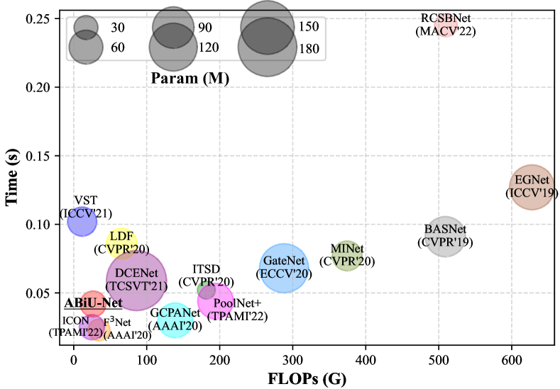
Figure 3: Visual comparison of ABiU-Net with some recent competitive methods in terms of parameters, FLOPs, and runtime.

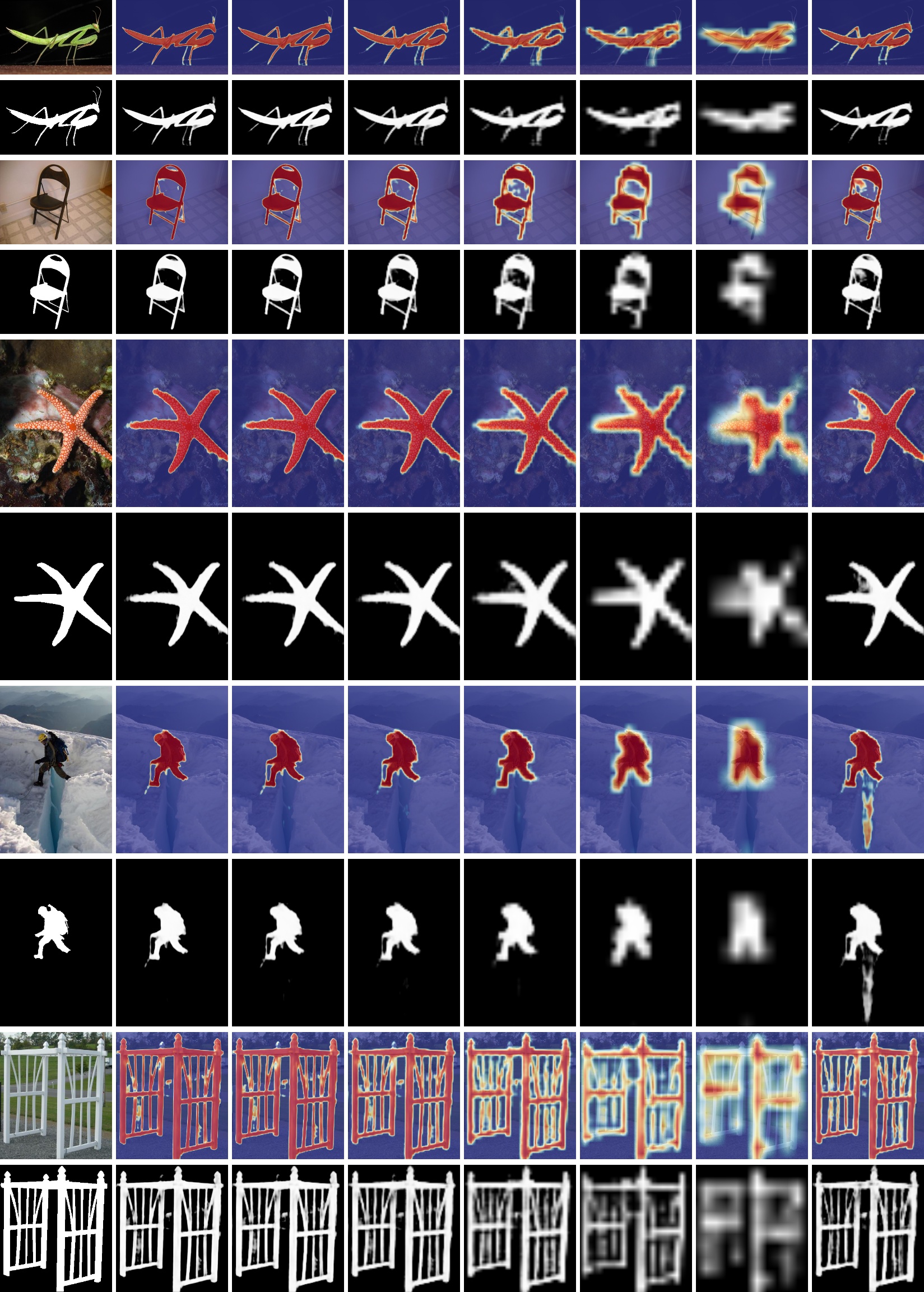
Img & GT     $\mathbf{P}^{H}_{1}$         $\mathbf{P}^{H}_{2}$         $\mathbf{P}^{H}_{3}$         $\mathbf{P}^{H}_{4}$         $\mathbf{P}^{H}_{5}$         $\mathbf{P}^{H}_{6}$         $\mathbf{P}^{T}$

Figure 4: Feature visualization maps and saliency maps of various intermediate side-outputs of ABiU-Net. Note that $\mathbf{P}^{H}_{1}$ is the final output saliency map.

Complex Scenes

 

Large Objects

 

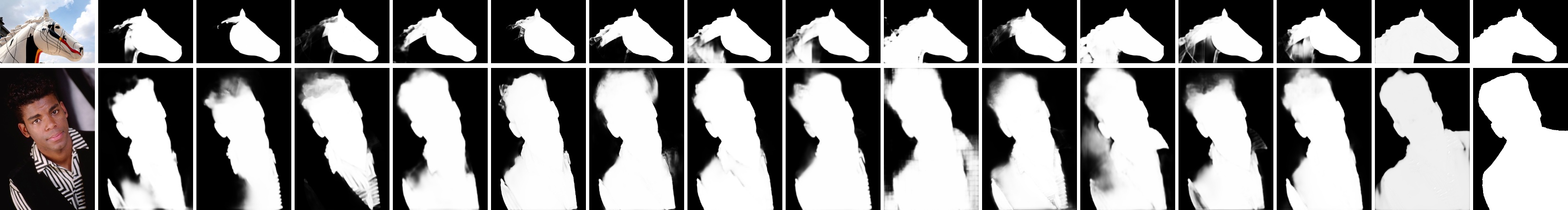
Small Objects

 

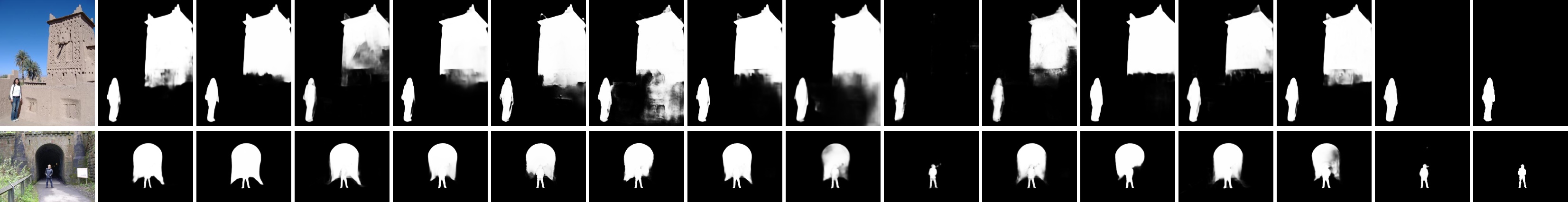
Thin Objects

 

Multiple Objects

 

Low Contrast

 

Confusing Backgrounds

 

Natural Phenomena

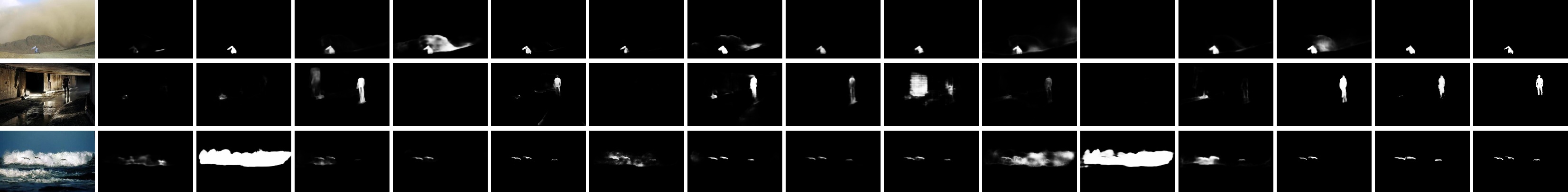
   Image        CPD      BASNet     EGNet      F3Net       ITSD       MINet       LDF      GCPANet     VST      PoolNet+   DCENet      DNA       ICON       Ours         GT

Figure 5: Qualitative comparison between ABiU-Net and 13 state-of-the-art SOD methods.

IV-B Performance Comparison

We compare the proposed ABiU-Net to previous state-of-the-art SOD methods, including UCF [25], SRM [26], PiCA [17], BRN [61], C2S [27], RAS [28], DSS [56], PAGE-Net [80], AFNet [48], DUCRF [49], HRSOD [81], CPD [32], BASNet [82], EGNet [33], F³Net [83], ITSD [50], MINet [51], LDF [84], GCPANet [53], GateNet [52], VST [41], DCENet [9], PoolNet+ [35], DNA [2], ICON [85], and RCSBNet [86]. For fair comparisons, the predicted saliency maps are downloaded from the official websites or produced by the released code with default settings. Note that we do not provide the results of MDF [91] on the HKU-IS [91] dataset because MDF adopts HKU-IS for training. For the same reason, we do not report the results of DHS [60] on the DUT-OMRON [93] dataset.

IV-B1 Quantitative Evaluation

The quantitative results of various methods in terms of $F_{\beta}$, MAE, $F_{\beta}^{\omega}$, and $S_{m}$ on six datasets are summarized in Table I. We can observe that the proposed ABiU-Net outperforms other methods by a large margin. Specifically, ABiU-Net attains $F_{\beta}$ values of 87.9%, 95.1%, 95.9%, 84.3%, 82.0%, and 90.6%, which are 0%, 0.9%, 0.8%, 2.1%, 0.3%, and 1.6% higher than the second-best results on SOD, HKU-IS, ECSSD, DUT-OMRON, THUR15K, and DUTS-test datasets, respectively. ABiU-Net also achieves the best MAE, i.e., 0.6%, 0.4%, 0.6%, 0.5%, and 0.6% better than the second-best results on HKU-IS, ECSSD, DUT-OMRON, THUR15K, and DUTS-test datasets, respectively. On the SOD dataset, the MAE value of ABiU-Net is a little worse than that of VST [41], ICON [85], and RCSBNet [86]. Moreover, the $F_{\beta}^{\omega}$ values of ABiU-Net are 1.9%, 1.7%, 3.9%, 2.6%, and 2.5% higher than the second-best results on HKU-IS, ECSSD, DUT-OMRON, THUR15K, and DUTS-test datasets, respectively. In terms of the metric $S_{m}$, ABiU-Net achieves the best performance in all datasets except for SOD. The $S_{m}$ values of ABiU-Net are 0.4%, 0.4%, 1.0%, 1.0%, and 0.3% higher than the second-best results on HKU-IS, ECSSD, DUT-OMRON, THUR15K, and DUTS-test datasets, respectively. Therefore, we can conclude that ABiU-Net has pushed forward the state-of-the-art for SOD significantly.

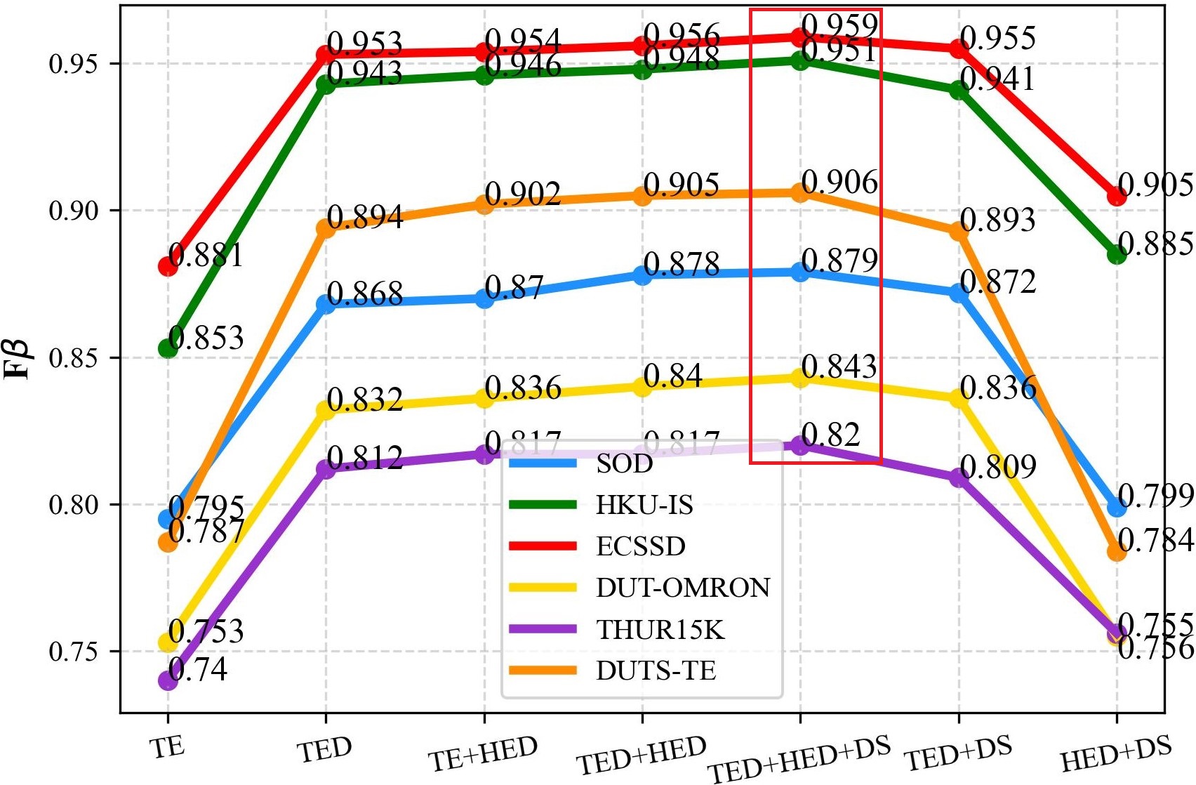
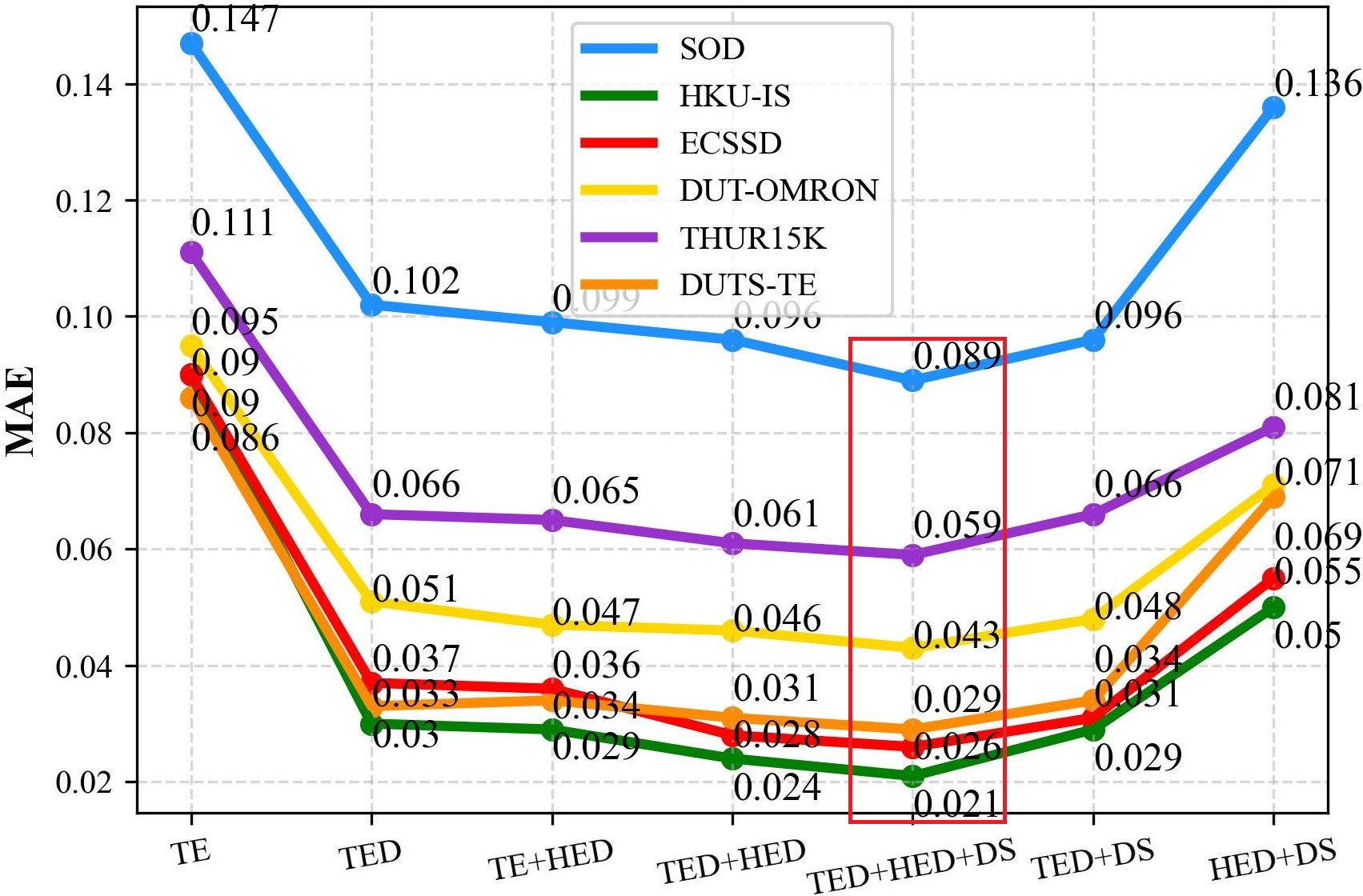
Figure 6: Effect of the main components of ABiU-Net. TE: TEncPath; TED: TEncPath + TDecPath; HED: HEncPath + HDecPath; DS: Deep Supervision.

TABLE II: Ablation studies for the deep supervision strategies of ABiU-Net.

	SOD		HKU-IS		ECSSD		DUT-OMRON		THUR15K		DUTS-test
Deep Supervision	$F_{\beta}$	MAE	$F_{\beta}$	MAE	$F_{\beta}$	MAE	$F_{\beta}$	MAE	$F_{\beta}$	MAE	$F_{\beta}$	MAE
{$\mathbf{P}^{H}_{1}$, $\mathbf{P}^{T}_{1}$}	.878	.096	.948	.024	.956	.028	.840	.046	.817	.061	.905	.031
{$\mathbf{P}^{H}_{i}$($i\in\{1,2,3,4,5,6\}$), $\mathbf{P}^{T}_{1}$}	.879	.089	.951	.021	.959	.026	.843	.043	.820	.059	.906	.029
{$\mathbf{P}^{H}_{i}$, $\mathbf{P}^{T}_{i}$($i\in\{1,2,3,4\}$)}	.875	.091	.948	.023	.959	.027	.841	.043	.817	.062	.906	.029
{$\mathbf{P}^{H}_{i}$($i\in\{1,2,3,4,5,6\}$), $\mathbf{P}^{T}_{i}$($i\in\{1,2,3,4\}$)}	.876	.092	.948	.024	.960	.027	.842	.043	.820	.062	.905	.030

• “{$\mathbf{P}^{H}_{i}$($i\in\{1,2,3,4,5,6\}$), $\mathbf{P}^{T}_{1}$}” means that the output saliency maps of all stages of HDecPath and the output saliency map of the last stage of TDecPath (i.e., $\mathbf{F}^{\rm TD}_{1}$) are supervised by ground-truth, which is the default deep supervision strategy of our ABiU-Net.

IV-B2 Complexity Analysis

Fig. 3 displays the complexity comparison between ABiU-Net and some recent competitive methods in terms of the number of parameters, the number of FLOPs, and runtime. Note that we use the same hardware setup (i.e., TITAN Xp GPU) and framework (i.e., PyTorch [87]) to test all methods for complexity analysis. It can be observed that the complexity of ABiU-Net is comparable to recent counterparts, exhibiting a relatively small number of parameters and FLOPs, as well as a relatively short runtime.

IV-B3 Qualitative Evaluation

In Fig. 4, we display some feature visualization figures and the corresponding saliency maps of various intermediate side-outputs to show how features evolve in ABiU-Net. From Fig. 4, it can be seen that the shapes of salient objects can be markedly refined from $\mathbf{P}^{H}_{6}$ to $\mathbf{P}^{H}_{1}$, which suggests the importance of the multi-level decoder in SOD. Moreover, the quality of saliency maps of $\mathbf{P}^{H}_{1}$ is far better than that of $\mathbf{P}^{T}$, which demonstrates the effectiveness of ABiU-Net in segmenting more accurate objects by learning complementary global and local information.

We proceed by displaying the qualitative comparisons in Fig. 5 to explicitly show the superiority of ABiU-Net over previous state-of-the-art SOD methods. Fig. 5 includes some representative images to incorporate various difficult circumstances, including complex scenes, large/small objects, thin objects, multiple objects, low-contrast scenes, and confusing backgrounds. Overall, ABiU-Net can generate better saliency maps in various scenarios. Surprisingly, ABiU-Net can even accurately segment salient objects with very complicated thin structures (the second thin sample), which is very challenging for all other methods. In addition, we also provide some representative images in the last group of Fig. 5 to show the results of ABiU-Net when being applied to natural phenomena like clouds, smoke, wave, and strong illumination at night. Overall, ABiU-Net can accurately segment salient objects under various natural phenomena. Overall, such a good visual performance of ABiU-Net benefits from its bilateral encoder/decoder structure. The communication between the two encoder/decoder paths facilitates ABiU-Net to accurately segment salient objects with fine details in various scenes, which is the core reason why our ABiU-Net can achieve such a good visual performance. In detail, the TEncPath/TDecPath of ABiU-Net can determine the coarse locations and shapes of salient objects, which is essential to find the large objects, multiple objects, and objects in complex, low-contrast or confusing background scenes. The HEncPath/HDecPath of ABiU-Net can model the local fine-grained representations to further refine salient object details guided by the coarse locations and shapes modeled by TEncPath/TDecPath, which is helpful to segment small/thin objects and distinguish the boundaries of salient objects.

TABLE III: Ablation studies for the hyper-parameters of ABiU-Net.

		SOD		HKU-IS		ECSSD		DUT-OMRON		THUR15K		DUTS-test
Configurations		$F_{\beta}$	MAE	$F_{\beta}$	MAE	$F_{\beta}$	MAE	$F_{\beta}$	MAE	$F_{\beta}$	MAE	$F_{\beta}$	MAE
Default Configurations		.879	.089	.951	.021	.959	.026	.843	.043	.820	.059	.906	.029
#Channels of HEncPath	(128, 128, 64, 32, 32, 8)	.879	.092	.951	.022	.958	.027	.839	.047	.814	.062	.901	.030
	(256, 128, 64, 32, 16, 8)	.879	.093	.951	.022	.959	.026	.843	.045	.815	.061	.904	.029
	(512, 256, 128, 64, 32, 16)	.877	.093	.951	.022	.958	.027	.839	.047	.815	.062	.904	.030
	(512, 256, 128, 128, 64, 16)	.881	.090	.950	.022	.959	.025	.836	.048	.814	.062	.901	.030
#Channels of TDecPath	(64, 32, 16, 8)	.878	.093	.951	.022	.957	.027	.844	.045	.817	.060	.907	.028
	(128, 32, 32, 8)	.868	.096	.951	.022	.957	.028	.841	.045	.818	.060	.907	.028
	(128, 128, 64, 16)	.876	.092	.951	.022	.958	.027	.842	.045	.818	.060	.907	.028
	(256, 128, 64, 32)	.871	.097	.951	.022	.959	.027	.844	.045	.817	.060	.907	.029
#Channels of HDecPath	(128, 64, 32, 16, 16, 8)	.875	.094	.950	.022	.959	.026	.843	.046	.816	.061	.905	.029
	(128, 128, 64, 32, 16, 8)	.880	.090	.951	.022	.958	.025	.840	.045	.815	.062	.906	.029
	(256, 256, 64, 32, 16, 8)	.874	.095	.951	.022	.958	.025	.846	.045	.813	.062	.904	.029
	(512, 256, 128, 64, 32, 16)	.872	.096	.950	.022	.959	.026	.840	.045	.815	.061	.906	.029

• “#Channels” means the number of channels. The default numbers of channels for HEncPath, TDecPath, and HDecPath are (256, 256, 128, 64, 64, 16), (128, 64, 32, 16), and (256, 128, 64, 32, 32, 8) from top to bottom, respectively.

IV-C Ablation Studies

In this section, we conduct extensive ablation studies for a better understanding of the proposed method.

IV-C1 Effect of Component Designs

We first evaluate the effect of the component designs of the proposed ABiU-Net. We start with the simple transformer-based encoder network without the decoder, i.e., TEncPath. We directly upsample the feature map from the last stage of the encoder for final prediction. The results are shown in the first column of Fig. 6 (i.e., TE). As can be seen, the performance is quite poor.

Effect of the Decoder

Then, we add a simple decoder, i.e., TDecPath (with the attention mechanism), to TEncPath, resulting in a transformer-based U-shaped encoder-decoder network. The evaluation results are put in the second column of Fig. 6 (i.e., TED). Significant performance boosting can be observed, which demonstrates that the encoder-decoder structure is necessary to utilize the low-level features for accurate SOD. The performance is even very competitive with recent state-of-the-art SOD methods, implying that the powerful global relationship modeling of vision transformers [39, 40, 6] is essential for SOD in discovering salient objects. The goal of this paper is to further boost the SOD performance upon this high baseline by combing the merits of vision transformers and CNNs.

Effect of the Asymmetric Bilateral Encoder

Next, we adopt TEncPath and HEncPath to build an asymmetric bilateral encoder. We also adopt HDecPath as the decoder, but the input of each stage in HDecPath is the outputs from HEncPath and the preceding decoder stage, excluding the output from TDecPath in ABiU-Net. The experimental results are displayed in the third column of Fig. 6 (i.e., TE+HED). We can observe a significant performance improvement. This experiment validates that our asymmetric bilateral encoder can supplement the transformer by complementary local representations, leading to higher SOD accuracy.

Effect of the Asymmetric Bilateral Decoder

We continue by adding TDecPath (with attention mechanism) to the model in Section IV-C1 to form the asymmetric bilateral decoder. The evaluation results are summarized in the fourth column of Fig. 6 (i.e., TED+HED). The asymmetric bilateral decoder can consistently improve the SOD accuracy. This experiment verifies that the asymmetric bilateral decoder is helpful in learning complementary information for both decoding the locations and fine details of salient objects.

Effect of Deep Supervision

At last, we add deep supervision as in Fig. 2 to obtain the final ABiU-Net. The results are shown in the fifth column of Fig. 6 (i.e., TED+HED+DS). Such default ABiU-Net achieves the best accuracy. Note that the fourth column is just ABiU-Net without deep supervision. From the fourth column to the fifth column, there is a significant performance improvement, indicating the effectiveness of training with deep supervision. Moreover, the default deep supervision strategy we used is to impose deep supervision on saliency maps of all stages of HDecPath (i.e., $\mathbf{P}^{H}_{i}$($i\in\{1,2,3,4,5,6\}$) while only on the saliency map of the last stage of TDecPath (i.e., $\mathbf{P}^{T}_{1}$). Intuitively, the reason for this design is that imposing deep supervision on all saliency maps of HDecPath can provide a direct supervision for each hidden layer of HDecPath (i.e., $\mathbf{F}^{\rm HD}_{6}$ $\sim$ $\mathbf{F}^{\rm HD}_{1}$). Moreover, this supervision can be easily propagated back to hidden layers of TDecPath to achieve the implicit optimization of all feature maps of TDecPath (i.e., $\mathbf{F}^{\rm TD}_{4}$ $\sim$ $\mathbf{F}^{\rm TD}_{1}$), because $\mathbf{F}^{\rm TD}_{4}$ $\sim$ $\mathbf{F}^{\rm TD}_{1}$ are the direct inputs of HDecPath to generate $\mathbf{F}^{\rm HD}_{6}$ $\sim$ $\mathbf{F}^{\rm HD}_{3}$. Hence, only supervising the output saliency map of the last stage of TDecPath rather than the saliency maps of all stages is enough to improve the discriminativeness of the hidden layer features of TDecPath.

In addition, we conduct the following ablation studies to further evaluate the effect of the different deep supervision strategies experimentally, whose results are shown in Table II. It is clear that all deep supervision strategies can boost the detection performance, and the model with the default deep supervision strategy can achieve the best overall performance.

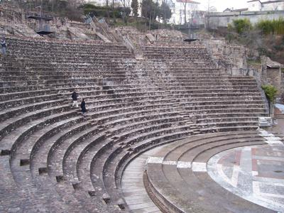
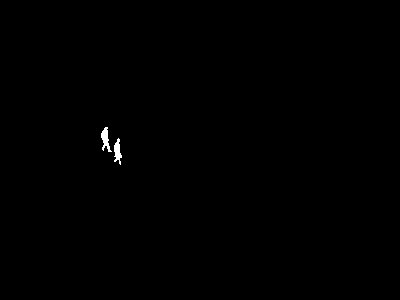
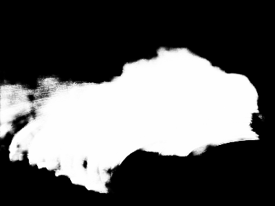
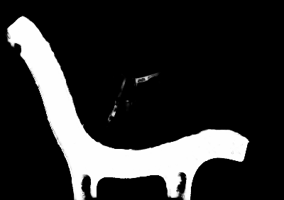
     Image             GT             Ours            Image            GT              Ours

Figure 7: Some failure cases of the proposed ABiU-Net. GT: Ground Truth.

Effect of Individual Transformer or CNN

The superiority of ABiU-Net over previous state-of-the-art methods is that ABiU-Net can make complementary use of the global contextual modeling ability of transformer and the local representation learning ability of CNNs. Next, we conduct ablation studies to evaluate the effect when the individual transformer or CNN is considered separately, and the results are displayed in the sixth and seventh columns of Fig. 6. It is clear that the individual transformer or CNN with the CA and DS (i.e., TED+DS or HED+DS) would produce worse results than the default ABiU-Net (i.e., TED+HED+DS). Hence, we can explicitly confirm the superiority of our asymmetric bilateral design. In addition, the CNN encoder path (i.e., HEncPath) is lightweight, so it can be optimized well with the large-scale SOD training data despite not being pre-trained on the ImageNet dataset [97].

IV-C2 Impact of Hyper-parameters

To explain how the default hyper-parameters of ABiU-Net are set, we evaluate the performance when varying hyper-parameters. Since PVT [70] is used as the TEncPath, we study the numbers of channels of HEncPath ($\mathbf{F}^{\rm HE}_{i}$), TDecPath ($\hat{\mathbf{F}}^{\rm TE}_{i}$), and HDecPath ($\hat{\mathbf{F}}^{\rm HE}_{i}$). We try some different settings, and the results are summarized in Table III. One can observe that ABiU-Net seems quite robust to various parameter settings as there is only a small performance fluctuation. This property makes that ABiU-Net has the potential to serve as a base architecture for SOD in the transformer era. Since the default parameter setting achieves slightly better performance, we use this setting by default.

IV-D Failure Case Analysis

Although our ABiU-Net achieves a new state of the art, it may still fail in some cases which are reported in Fig. 7. As can be seen from the two examples in the first row of Fig. 7, our ABiU-Net may fail for tiny objects and less inconspicuous objects. From the two examples in the second row, we can see that the partial regions within some saliency objects are particularly prominent, resulting in the failure of our ABiU-Net which may only segment the more prominent regions. Hence, how to ensure the integrity of salient objects is the next problem to be solved. Moreover, as shown in the third row of Fig. 7, when the background regions are particularly complex, especially containing objects belonging to the same semantic categories as salient objects, our method may fail to distinguish the salient objects from background regions. Furthermore, the salient objects in an image of the datasets are subjectively labeled and it may be ambiguous which objects are salient in a few images. In this case, our ABiU-Net may detect other objects in an image to be salient, rather than the ground-truth salient objects, as shown in the fourth row of Fig. 7. Based on the above analysis, we can conclude that there is still a long way towards the ideal SOD solution.

V Conclusion

This paper focuses on boosting SOD accuracy with the vision transformer [39, 40]. It is widely accepted that vision transformers are adept at learning global contextual information that is essential for locating salient objects, while CNNs have a strong ability to learn local fine-grained information that is necessary for refining object details [1, 16, 17]. Therefore, this paper explores the combination of the transformer and CNN to learn discriminative hybrid features for accurate SOD. For this goal, we design the Asymmetric Bilateral U-Net (ABiU-Net), where both the encoder and decoder have two paths. Extensive experiments demonstrate that ABiU-Net can significantly improve SOD performance when compared with state-of-the-art methods. Considering that ABiU-Net is an elegant architecture without carefully designed modules or engineering skills, ABiU-Net provides a new perspective for SOD in the transformer era.

Yu Qiu received her BEng degree from Northwest A&F University in 2017, and her Ph.D. degree from Nankai University in 2022. Currently, she is a postdoctoral scholar at the College of Artificial Intelligence, Nankai University. Her research interests include computer vision and machine learning.

Yun Liu received his BEng and Ph.D. degrees from Nankai University in 2016 and 2020, respectively. Then, he worked with Prof. Luc Van Gool for one and a half years as a postdoctoral scholar at Computer Vision Lab, ETH Zurich. Currently, he is a scientist at Institute for Infocomm Research (I2R), A*STAR. His research interests include computer vision and machine learning.

Le Zhang received the BEng degree from the University of Electronic Science and Technology of China, in 2011, and the MSc and Ph.D. degrees from Nanyang Technological University (NTU), in 2012 and 2016, respectively. Currently, he is a professor at the University of Electronic Science and Technology of China. He served as the TPC member in several conferences such as AAAI, IJCAI. He has served as a guest editor for Pattern Recognition and Neurocomputing. His current research interests include deep learning and computer vision.

Haotian Lu is studying at the College of Artificial Intelligence, Nankai University. He graduated from Taiyuan University of Technology with a bachelor’s degree in 2022. His research interests include computer vision and medical image processing.

Jing Xu is a professor at the College of Artificial Intelligence, Nankai University. She received her Ph.D. degree from Nankai University in 2003. She has published more than 100 papers in software engineering, software security, and big data analytics. She won the second prize of the Tianjin Science and Technology Progress Award twice in 2017 and 2018, respectively.

References

- [1] M.-M. Cheng, N. J. Mitra, X. Huang, P. H. Torr, and S.-M. Hu, “Global contrast based salient region detection,” IEEE Trans. Pattern Anal. Mach. Intell. (TPAMI), vol. 37, no. 3, pp. 569–582, 2014.
- [2] Y. Liu, M.-M. Cheng, X.-Y. Zhang, G.-Y. Nie, and M. Wang, “DNA: Deeply supervised nonlinear aggregation for salient object detection,” IEEE Trans. Cybernetics (TCYB), vol. 52, no. 7, pp. 6131–6142, 2021.
- [3] Y. Liu, Y.-C. Gu, X.-Y. Zhang, W. Wang, and M.-M. Cheng, “Lightweight salient object detection via hierarchical visual perception learning,” IEEE Trans. Cybernetics (TCYB), vol. 51, no. 9, pp. 4439–4449, 2020.
- [4] L. Wang, R. Chen, L. Zhu, H. Xie, and X. Li, “Deep sub-region network for salient object detection,” IEEE Trans. Circ. Syst. Video Technol. (TCSVT), vol. 31, no. 2, pp. 728–741, 2021.
- [5] Z. Tu, Y. Ma, C. Li, J. Tang, and B. Luo, “Edge-guided non-local fully convolutional network for salient object detection,” IEEE Trans. Circ. Syst. Video Technol. (TCSVT), vol. 31, no. 2, pp. 582–593, 2021.
- [6] Z. Li, C. Lang, L. Liang, J. Zhao, S. Feng, Q. Hou, and J. Feng, “Dense attentive feature enhancement for salient object detection,” IEEE Trans. Circ. Syst. Video Technol. (TCSVT), vol. 32, no. 12, pp. 8128–8141, 2022.
- [7] L. Zhang, Q. Zhang, and R. Zhao, “Progressive dual-attention residual network for salient object detection,” IEEE Trans. Circ. Syst. Video Technol. (TCSVT), vol. 32, no. 9, pp. 5902–5915, 2022.
- [8] Q. Zhang, R. Zhao, and L. Zhang, “TCRNet: A trifurcated cascaded refinement network for salient object detection,” IEEE Trans. Circ. Syst. Video Technol. (TCSVT), vol. 33, no. 1, pp. 298–311, 2023.
- [9] H. Mei, Y. Liu, Z. Wei, D. Zhou, X. Wei, Q. Zhang, and X. Yang, “Exploring dense context for salient object detection,” IEEE Trans. Circ. Syst. Video Technol. (TCSVT), vol. 32, no. 3, pp. 1378–1389, 2021.
- [10] D. Meger, P.-E. Forssén, K. Lai, S. Helmer, S. McCann, T. Southey, M. Baumann, J. J. Little, and D. G. Lowe, “Curious george: An attentive semantic robot,” Robotics and Autonomous Systems, vol. 56, no. 6, pp. 503–511, 2008.
- [11] M.-M. Cheng, F.-L. Zhang, N. J. Mitra, X. Huang, and S.-M. Hu, “RepFinder: finding approximately repeated scene elements for image editing,” ACM Trans. Graph. (TOG), vol. 29, no. 4, pp. 83:1–83:8, 2010.
- [12] Y. Gao, M. Wang, Z.-J. Zha, J. Shen, X. Li, and X. Wu, “Visual-textual joint relevance learning for tag-based social image search,” IEEE Trans. Image Process. (TIP), vol. 22, no. 1, pp. 363–376, 2013.
- [13] Z. Ren, S. Gao, L.-T. Chia, and I. W.-H. Tsang, “Region-based saliency detection and its application in object recognition,” IEEE Trans. Circ. Syst. Video Technol. (TCSVT), vol. 24, no. 5, pp. 769–779, 2013.
- [14] L. Marchesotti, C. Cifarelli, and G. Csurka, “A framework for visual saliency detection with applications to image thumbnailing,” in Int. Conf. Comput. Vis. (ICCV), 2009, pp. 2232–2239.
- [15] Y. Liu, Y.-H. Wu, P.-S. Wen, Y.-J. Shi, Y. Qiu, and M.-M. Cheng, “Leveraging instance-, image- and dataset-level information for weakly supervised instance segmentation,” IEEE Trans. Pattern Anal. Mach. Intell. (TPAMI), 2020.
- [16] Z. Luo, A. K. Mishra, A. Achkar, J. A. Eichel, S. Li, and P.-M. Jodoin, “Non-local deep features for salient object detection,” in IEEE Conf. Comput. Vis. Pattern Recog. (CVPR), 2017, pp. 6609–6617.
- [17] N. Liu, J. Han, and M.-H. Yang, “PiCANet: Learning pixel-wise contextual attention for saliency detection,” in IEEE Conf. Comput. Vis. Pattern Recog. (CVPR), 2018, pp. 3089–3098.
- [18] X. Hu, C.-W. Fu, L. Zhu, T. Wang, and P.-A. Heng, “SAC-Net: Spatial attenuation context for salient object detection,” IEEE Trans. Circ. Syst. Video Technol. (TCSVT), vol. 31, no. 3, pp. 1079–1090, 2021.
- [19] Q. Zhang, M. Duanmu, Y. Luo, Y. Liu, and J. Han, “Engaging part-whole hierarchies and contrast cues for salient object detection,” IEEE Trans. Circ. Syst. Video Technol. (TCSVT), vol. 32, no. 6, pp. 3644–3658, 2022.
- [20] L. Wang, H. Lu, X. Ruan, and M.-H. Yang, “Deep networks for saliency detection via local estimation and global search,” in IEEE Conf. Comput. Vis. Pattern Recog. (CVPR), 2015, pp. 3183–3192.
- [21] G. Lee, Y.-W. Tai, and J. Kim, “Deep saliency with encoded low level distance map and high level features,” in IEEE Conf. Comput. Vis. Pattern Recog. (CVPR), 2016, pp. 660–668.
- [22] L. Wang, L. Wang, H. Lu, P. Zhang, and X. Ruan, “Saliency detection with recurrent fully convolutional networks,” in Eur. Conf. Comput. Vis. (ECCV), 2016, pp. 825–841.
- [23] G. Li and Y. Yu, “Deep contrast learning for salient object detection,” in IEEE Conf. Comput. Vis. Pattern Recog. (CVPR), 2016, pp. 478–487.
- [24] P. Zhang, D. Wang, H. Lu, H. Wang, and X. Ruan, “Amulet: Aggregating multi-level convolutional features for salient object detection,” in Int. Conf. Comput. Vis. (ICCV), 2017, pp. 202–211.
- [25] P. Zhang, D. Wang, H. Lu, H. Wang, and B. Yin, “Learning uncertain convolutional features for accurate saliency detection,” in Int. Conf. Comput. Vis. (ICCV), 2017, pp. 212–221.
- [26] T. Wang, A. Borji, L. Zhang, P. Zhang, and H. Lu, “A stagewise refinement model for detecting salient objects in images,” in Int. Conf. Comput. Vis. (ICCV), 2017, pp. 4019–4028.
- [27] X. Li, F. Yang, H. Cheng, W. Liu, and D. Shen, “Contour knowledge transfer for salient object detection,” in Eur. Conf. Comput. Vis. (ECCV), 2018, pp. 355–370.
- [28] S. Chen, X. Tan, B. Wang, and X. Hu, “Reverse attention for salient object detection,” in Eur. Conf. Comput. Vis. (ECCV), 2018, pp. 234–250.
- [29] Y. Liu, X.-Y. Zhang, J.-W. Bian, L. Zhang, and M.-M. Cheng, “SAMNet: Stereoscopically attentive multi-scale network for lightweight salient object detection,” IEEE Trans. Image Process. (TIP), vol. 30, pp. 3804–3814, 2021.
- [30] Y. Qiu, Y. Liu, X. Ma, L. Liu, H. Gao, and J. Xu, “Revisiting multi-level feature fusion: A simple yet effective network for salient object detection,” in Int. Conf. Image Process. (ICIP), 2019, pp. 4010–4014.
- [31] Y. Qiu, Y. Liu, H. Yang, and J. Xu, “A simple saliency detection approach via automatic top-down feature fusion,” Neurocomputing, vol. 388, pp. 124–134, 2020.
- [32] Z. Wu, L. Su, and Q. Huang, “Cascaded partial decoder for fast and accurate salient object detection,” in IEEE Conf. Comput. Vis. Pattern Recog. (CVPR), 2019, pp. 3907–3916.
- [33] J.-X. Zhao, J. Liu, D.-P. Fan, Y. Cao, J. Yang, and M.-M. Cheng, “EGNet: Edge guidance network for salient object detection,” in Int. Conf. Comput. Vis. (ICCV), 2019, pp. 8779–8788.
- [34] Y. Qiu, Y. Liu, S. Li, and J. Xu, “MiniSeg: An extremely minimum network for efficient COVID-19 segmentation,” in AAAI Conf. Artif. Intell. (AAAI), 2021, pp. 4846–4854.
- [35] J.-J. Liu, Q. Hou, Z.-A. Liu, and M.-M. Cheng, “PoolNet+: Exploring the potential of pooling for salient object detection,” IEEE Trans. Pattern Anal. Mach. Intell. (TPAMI), vol. 45, no. 1, pp. 887–904, 2022.
- [36] L. Sun, Z. Chen, Q. J. Wu, H. Zhao, W. He, and X. Yan, “AMPNet: Average-and max-pool networks for salient object detection,” IEEE Trans. Circ. Syst. Video Technol. (TCSVT), vol. 31, no. 11, pp. 4321–4333, 2021.
- [37] C. Zhang, S. Gao, D. Mao, and Y. Zhou, “DHNet: Salient object detection with dynamic scale-aware learning and hard-sample refinement,” IEEE Trans. Circ. Syst. Video Technol. (TCSVT), vol. 32, no. 11, pp. 7772–7782, 2022.
- [38] K. He, X. Zhang, S. Ren, and J. Sun, “Deep residual learning for image recognition,” in IEEE Conf. Comput. Vis. Pattern Recog. (CVPR), 2016, pp. 770–778.
- [39] A. Vaswani, N. Shazeer, N. Parmar, J. Uszkoreit, L. Jones, A. N. Gomez, L. Kaiser, and I. Polosukhin, “Attention is all you need,” in Annu. Conf. Neur. Inform. Process. Syst. (NeurIPS), 2017, pp. 6000–6010.
- [40] A. Dosovitskiy, L. Beyer, A. Kolesnikov, D. Weissenborn, X. Zhai, T. Unterthiner, M. Dehghani, M. Minderer, G. Heigold, S. Gelly, J. Uszkoreit, and N. Houlsby, “An image is worth 16x16 words: Transformers for image recognition at scale,” in Int. Conf. Learn. Represent. (ICLR), 2021.
- [41] N. Liu, N. Zhang, K. Wan, L. Shao, and J. Han, “Visual saliency transformer,” in Int. Conf. Comput. Vis. (ICCV), 2021, pp. 4722–4732.
- [42] Y. Mao, J. Zhang, Z. Wan, Y. Dai, A. Li, Y. Lv, X. Tian, D.-P. Fan, and N. Barnes, “Transformer transforms salient object detection and camouflaged object detection,” arXiv preprint arXiv:2104.10127, 2021.
- [43] B. Hariharan, P. Arbeláez, R. Girshick, and J. Malik, “Hypercolumns for object segmentation and fine-grained localization,” in IEEE Conf. Comput. Vis. Pattern Recog. (CVPR), 2015, pp. 447–456.
- [44] Y. Zeng, H. Lu, L. Zhang, M. Feng, and A. Borji, “Learning to promote saliency detectors,” in IEEE Conf. Comput. Vis. Pattern Recog. (CVPR), 2018, pp. 1644–1653.
- [45] T. Zhao and X. Wu, “Pyramid feature attention network for saliency detection,” in IEEE Conf. Comput. Vis. Pattern Recog. (CVPR), 2019, pp. 3085–3094.
- [46] J. Su, J. Li, Y. Zhang, C. Xia, and Y. Tian, “Selectivity or invariance: Boundary-aware salient object detection,” in Int. Conf. Comput. Vis. (ICCV), 2019, pp. 3799–3808.
- [47] O. Ronneberger, P. Fischer, and T. Brox, “U-Net: Convolutional networks for biomedical image segmentation,” in Int. Conf. Med. Image Comp. Comput.-Assist. Interv. (MICCAI), 2015, pp. 234–241.
- [48] M. Feng, H. Lu, and E. Ding, “Attentive feedback network for boundary-aware salient object detection,” in IEEE Conf. Comput. Vis. Pattern Recog. (CVPR), 2019, pp. 1623–1632.
- [49] Y. Xu, D. Xu, X. Hong, W. Ouyang, R. Ji, M. Xu, and G. Zhao, “Structured modeling of joint deep feature and prediction refinement for salient object detection,” in Int. Conf. Comput. Vis. (ICCV), 2019, pp. 3789–3798.
- [50] H. Zhou, X. Xie, J.-H. Lai, Z. Chen, and L. Yang, “Interactive two-stream decoder for accurate and fast saliency detection,” in IEEE Conf. Comput. Vis. Pattern Recog. (CVPR), 2020, pp. 9141–9150.
- [51] Y. Pang, X. Zhao, L. Zhang, and H. Lu, “Multi-scale interactive network for salient object detection,” in IEEE Conf. Comput. Vis. Pattern Recog. (CVPR), 2020, pp. 9413–9422.
- [52] X. Zhao, Y. Pang, L. Zhang, H. Lu, and L. Zhang, “Suppress and balance: A simple gated network for salient object detection,” in Eur. Conf. Comput. Vis. (ECCV). Springer, 2020, pp. 35–51.
- [53] Z. Chen, Q. Xu, R. Cong, and Q. Huang, “Global context-aware progressive aggregation network for salient object detection,” AAAI Conf. Artif. Intell. (AAAI), 2020.
- [54] C. Yu, J. Wang, C. Peng, C. Gao, G. Yu, and N. Sang, “BiSeNet: Bilateral segmentation network for real-time semantic segmentation,” in Eur. Conf. Comput. Vis. (ECCV), 2018, pp. 325–341.
- [55] S. Xie and Z. Tu, “Holistically-nested edge detection,” in Int. Conf. Comput. Vis. (ICCV), 2015, pp. 1395–1403.
- [56] Q. Hou, M.-M. Cheng, X. Hu, A. Borji, Z. Tu, and P. Torr, “Deeply supervised salient object detection with short connections,” IEEE Trans. Pattern Anal. Mach. Intell. (TPAMI), vol. 41, no. 4, pp. 815–828, 2019.
- [57] J. Chen, Y. Lu, Q. Yu, X. Luo, E. Adeli, Y. Wang, L. Lu, A. L. Yuille, and Y. Zhou, “TransUNet: Transformers make strong encoders for medical image segmentation,” arXiv preprint arXiv:2102.04306, 2021.
- [58] H. Cao, Y. Wang, J. Chen, D. Jiang, X. Zhang, Q. Tian, and M. Wang, “Swin-Unet: Unet-like pure transformer for medical image segmentation,” arXiv preprint arXiv:2105.05537, 2021.
- [59] A. Lin, B. Chen, J. Xu, Z. Zhang, G. Lu, and D. Zhang, “DS-TransUNet: Dual swin transformer U-Net for medical image segmentation,” IEEE Trans. Inst. and Measure. (TIM), 2022.
- [60] N. Liu and J. Han, “DHSNet: Deep hierarchical saliency network for salient object detection,” in IEEE Conf. Comput. Vis. Pattern Recog. (CVPR), 2016, pp. 678–686.
- [61] T. Wang, L. Zhang, S. Wang, H. Lu, G. Yang, X. Ruan, and A. Borji, “Detect globally, refine locally: A novel approach to saliency detection,” in IEEE Conf. Comput. Vis. Pattern Recog. (CVPR), 2018, pp. 3127–3135.
- [62] X. Zhang, T. Wang, J. Qi, H. Lu, and G. Wang, “Progressive attention guided recurrent network for salient object detection,” in IEEE Conf. Comput. Vis. Pattern Recog. (CVPR), 2018, pp. 714–722.
- [63] Y.-H. Wu, Y. Liu, L. Zhang, M.-M. Cheng, and B. Ren, “EDN: Salient object detection via extremely-downsampled network,” IEEE Trans. Image Process. (TIP), vol. 31, pp. 3125–3136, 2022.
- [64] Y. Gu, L. Wang, Z. Wang, Y. Liu, M.-M. Cheng, and S.-P. Lu, “Pyramid constrained self-attention network for fast video salient object detection,” in AAAI Conf. Artif. Intell. (AAAI), 2020, pp. 10 869–10 876.
- [65] Y. Qiu, Y. Liu, Y. Chen, J. Zhang, J. Zhu, and J. Xu, “A2SPPNet: Attentive atrous spatial pyramid pooling network for salient object detection,” IEEE Trans. Multimedia (TMM), 2022.
- [66] L.-C. Chen, G. Papandreou, I. Kokkinos, K. Murphy, and A. L. Yuille, “DeepLab: Semantic image segmentation with deep convolutional nets, atrous convolution, and fully connected CRFs,” IEEE Trans. Pattern Anal. Mach. Intell. (TPAMI), vol. 40, no. 4, pp. 834–848, 2017.
- [67] W. Wang, Q. Lai, H. Fu, J. Shen, H. Ling, and R. Yang, “Salient object detection in the deep learning era: An in-depth survey,” IEEE Trans. Pattern Anal. Mach. Intell. (TPAMI), vol. 44, no. 6, pp. 3239–3259, 2021.
- [68] O. Russakovsky, J. Deng, H. Su, J. Krause, S. Satheesh, S. Ma, Z. Huang, A. Karpathy, A. Khosla, M. Bernstein et al., “ImageNet large scale visual recognition challenge,” Int. J. Comput. Vis. (IJCV), vol. 115, no. 3, pp. 211–252, 2015.
- [69] L. Yuan, Y. Chen, T. Wang, W. Yu, Y. Shi, Z.-H. Jiang, F. E. Tay, J. Feng, and S. Yan, “Tokens-to-token ViT: Training vision transformers from scratch on ImageNet,” in Int. Conf. Comput. Vis. (ICCV), 2021, pp. 558–567.
- [70] W. Wang, E. Xie, X. Li, D.-P. Fan, K. Song, D. Liang, T. Lu, P. Luo, and L. Shao, “Pyramid vision transformer: A versatile backbone for dense prediction without convolutions,” in Int. Conf. Comput. Vis. (ICCV), 2021, pp. 568–578.
- [71] Z. Liu, Y. Lin, Y. Cao, H. Hu, Y. Wei, Z. Zhang, S. Lin, and B. Guo, “Swin transformer: Hierarchical vision transformer using shifted windows,” in Int. Conf. Comput. Vis. (ICCV), 2021, pp. 10 012–10 022.
- [72] Y.-H. Wu, Y. Liu, X. Zhan, and M.-M. Cheng, “P2T: Pyramid pooling transformer for scene understanding,” IEEE Trans. Pattern Anal. Mach. Intell. (TPAMI), 2022.
- [73] K. Han, A. Xiao, E. Wu, J. Guo, C. Xu, and Y. Wang, “Transformer in transformer,” Annu. Conf. Neur. Inform. Process. Syst. (NeurIPS), vol. 34, pp. 15 908–15 919, 2021.
- [74] Y. Cui, “Dynamic feature aggregation for efficient video object detection,” in Asian Conf. Comput. Vis. (ACCV), 2022, pp. 944–960.
- [75] ——, “Feature aggregated queries for transformer-based video object detectors,” in IEEE Conf. Comput. Vis. Pattern Recog. (CVPR), 2023, pp. 6365–6376.
- [76] Y. Mao, J. Zhang, Z. Wan, Y. Dai, A. Li, Y. Lv, X. Tian, D.-P. Fan, and N. Barnes, “Generative transformer for accurate and reliable salient object detection,” arXiv preprint arXiv:2104.10127, 2021.
- [77] C.-Y. Lee, S. Xie, P. Gallagher, Z. Zhang, and Z. Tu, “Deeply-supervised nets,” in Artif. Intell. Stat. (AISTATS), 2015, pp. 562–570.
- [78] H. Zhao, J. Shi, X. Qi, X. Wang, and J. Jia, “Pyramid scene parsing network,” in IEEE Conf. Comput. Vis. Pattern Recog. (CVPR), 2017, pp. 2881–2890.
- [79] J. Hu, L. Shen, and G. Sun, “Squeeze-and-excitation networks,” in IEEE Conf. Comput. Vis. Pattern Recog. (CVPR), 2018, pp. 7132–7141.
- [80] W. Wang, S. Zhao, J. Shen, S. C. Hoi, and A. Borji, “Salient object detection with pyramid attention and salient edges,” in IEEE Conf. Comput. Vis. Pattern Recog. (CVPR), 2019, pp. 1448–1457.
- [81] Y. Zeng, P. Zhang, J. Zhang, Z. Lin, and H. Lu, “Towards high-resolution salient object detection,” in Int. Conf. Comput. Vis. (ICCV), 2019, pp. 7234–7243.
- [82] X. Qin, Z. Zhang, C. Huang, C. Gao, M. Dehghan, and M. Jagersand, “BASNet: Boundary-aware salient object detection,” in IEEE Conf. Comput. Vis. Pattern Recog. (CVPR), 2019, pp. 7479–7489.
- [83] J. Wei, S. Wang, and Q. Huang, “F3Net: Fusion, feedback and focus for salient object detection,” in AAAI Conf. Artif. Intell. (AAAI), 2020.
- [84] J. Wei, S. Wang, Z. Wu, C. Su, Q. Huang, and Q. Tian, “Label decoupling framework for salient object detection,” in IEEE Conf. Comput. Vis. Pattern Recog. (CVPR), 2020, pp. 13 025–13 034.
- [85] M. Zhuge, D.-P. Fan, N. Liu, D. Zhang, D. Xu, and L. Shao, “Salient object detection via integrity learning,” IEEE Trans. Pattern Anal. Mach. Intell. (TPAMI), 2022.
- [86] Y. Y. Ke and T. Tsubono, “Recursive contour-saliency blending network for accurate salient object detection,” in IEEE Winter Conf. App. Comput. Vis. (WACV), 2022, pp. 2940–2950.
- [87] A. Paszke, S. Gross, F. Massa, A. Lerer, J. Bradbury, G. Chanan, T. Killeen, Z. Lin, N. Gimelshein, L. Antiga et al., “PyTorch: An imperative style, high-performance deep learning library,” in Annu. Conf. Neur. Inform. Process. Syst. (NeurIPS), 2019, pp. 8026–8037.
- [88] I. Loshchilov and F. Hutter, “Decoupled weight decay regularization,” in Int. Conf. Learn. Represent. (ICLR), 2019.
- [89] L. Wang, H. Lu, Y. Wang, M. Feng, D. Wang, B. Yin, and X. Ruan, “Learning to detect salient objects with image-level supervision,” in IEEE Conf. Comput. Vis. Pattern Recog. (CVPR), 2017, pp. 136–145.
- [90] V. Movahedi and J. H. Elder, “Design and perceptual validation of performance measures for salient object segmentation,” in IEEE Conf. Comput. Vis. Pattern Recog. (CVPR), 2010, pp. 49–56.
- [91] G. Li and Y. Yu, “Visual saliency based on multiscale deep features,” in IEEE Conf. Comput. Vis. Pattern Recog. (CVPR), 2015, pp. 5455–5463.
- [92] Q. Yan, L. Xu, J. Shi, and J. Jia, “Hierarchical saliency detection,” in IEEE Conf. Comput. Vis. Pattern Recog. (CVPR), 2013, pp. 1155–1162.
- [93] C. Yang, L. Zhang, H. Lu, X. Ruan, and M.-H. Yang, “Saliency detection via graph-based manifold ranking,” in IEEE Conf. Comput. Vis. Pattern Recog. (CVPR), 2013, pp. 3166–3173.
- [94] M.-M. Cheng, N. J. Mitra, X. Huang, and S.-M. Hu, “SalientShape: Group saliency in image collections,” The Vis. Comput. (TVCJ), vol. 30, no. 4, pp. 443–453, 2014.
- [95] R. Margolin, L. Zelnik-Manor, and A. Tal, “How to evaluate foreground maps?” in IEEE Conf. Comput. Vis. Pattern Recog. (CVPR), 2014, pp. 248–255.
- [96] D.-P. Fan, M.-M. Cheng, Y. Liu, T. Li, and A. Borji, “Structure-measure: A new way to evaluate foreground maps,” in Int. Conf. Comput. Vis. (ICCV), 2017, pp. 4548–4557.
- [97] K. He, R. Girshick, and P. Dollár, “Rethinking ImageNet pre-training,” in Int. Conf. Comput. Vis. (ICCV), 2019, pp. 4918–4927.