Higher Order Derivative-Based Receiver Pre-processing for Molecular Communications

Abstract

While molecular communication via diffusion experiences significant inter-symbol interference (ISI), recent work suggests that ISI can be mitigated via time differentiation pre-processing which achieves pulse narrowing. Herein, the approach is generalized to higher order differentiation. The fundamental trade-off between ISI mitigation and noise amplification is characterized, showing the existence of an optimal derivative order that minimizes the bit error rate (BER). Theoretical analyses of the BER and a signal-to-interference-plus-noise ratio are provided, the derivative order optimization problem is posed and solved for threshold-based detectors. For more complex detectors which exploit a window memory, it is shown that derivative pre-processing can strongly reduce the size of the needed window. Extensive numerical results confirm the accuracy of theoretical derivations, the gains in performance via derivative pre-processing over other methods and the impact of the optimal derivative order. Derivative pre-processing offers a low complexity/high-performance method for reducing ISI at the expense of increased transmission power to reduce noise amplification.

I Introduction

Molecular communication via diffusion (MCD) enables communication through the emission of chemical (molecular) signals [3]. In an MCD system, the information is encoded into a physical property of the molecular signal such as its emission intensity [4], emitted molecule type [5], time of emission [6], spatial location of emission [7, 8], or a combination of these signaling degrees of freedom [7, 8, 9, 10, 11]. After their emission from the transmitter, the messenger molecules randomly propagate in the fluid communication medium, exhibiting Brownian motion [12]. This stochasticity causes some molecules to never arrive at the receiver, and creates delays in some molecules that do arrive. From a communications engineering perspective, the molecules that arrive later than intended cause inter-symbol interference (ISI). ISI is the leading cause of the notoriously low data rates of MCD.

The ISI problem has been tackled through both transmitter and receiver side solutions. In particular, single- or multi-molecule modulation schemes have been considered [13], source and channel codes have been designed [14], as well as transmitter-side pre-equalization approaches [15, 11]. At the receiver side, the maximum a posteriori (MAP) and maximum likelihood (ML) sequence detectors are considered by [16], as well as decision feedback and minimum mean squared error (MMSE) equalizers that account for ISI. Inspired by the computational constraints of a nano-machine, a low complexity, adaptive threshold detector is presented in [17]. In [18], a decision feedback mechanism is utilized to estimate ISI and aid a symbol-by-symbol detector (memory limited decision aided decoder, MLDA). A similar decision feedback mechanism is also used in [19] in the context of a sequential probability ratio test-based MCD detector.

Recently, it was shown in [20] that applying a single discrete-time derivative on the received signal mitigates ISI in concentration-based synthetic MCD. Subsequently, a rising-edge-based detection with differentiation strategy was devised in [21] for macro-scale molecular MIMO. In [20], it was shown that a single differentiation narrowed the received signal pulse thus mitigating ISI. Herein, we consider multiple orders of differentiation and their pairing with a variety of detector strategies as noted below. It should be observed that differentiation is not only an engineered mechanism for micro-or nano-machines, but is a processing/sensing that occurs in organisms. In particular, bacterial responses are affected by the rate of change of physical and biochemical quantities. Examples include detecting spatial gradients of bio-molecule concentration used for chemotaxis [22] and the varying effect of heating rate in protein synthesis [23, 24].

In our preliminary study [1], we had introduced the higher order derivative concept, discussed its fundamental trade-off between ISI mitigation and noise amplification, and introduced a lower complexity, banded alternative to the optimal maximum likelihood sequence detector that exploits the ISI mitigation offered by higher order differentiation. In addition, in a separate preliminary study [2], we had improved the fixed threshold detector used by [20] for $m=1$ and [1] for $m\geq 1$, and provided an objective function to optimize the derivative order $m$ using the new fixed threshold detector. This paper extends and completes these two works by providing complete derivations and proofs, deriving the theoretical bit error ratio (BER) of the detector proposed in [2], introducing a new detector to be paired with the derivative operator, as well as addressing the computational complexities of the detectors and the asymptotic relationship between derivative orders. The contributions of this paper are as follows:

1. We generalize the initial endeavors of [20] to a pre-processor with an arbitrary derivative order $m$.

2. We characterize the fundamental trade-off of the derivative-based pre-processing framework between ISI mitigation and noise amplification.

3. Framing the derivative operation as a receiver pre-processor block that takes place before detection, we present several derivative operator-detector pairs. To this end, we provide the limited-memory, banded version of the MLSD, generalize the MLDA to an arbitrary derivative order, and adapt two threshold-based detectors to the derivative pre-processor.

4. We derive the theoretical bit error ratio (BER) expressions for the threshold-based detectors.

5. We provide a signal-to-interference-plus-noise ratio-like (SINR) objective function that is compatible with an arbitrary derivative order. Through this objective function and the theoretical error expression, we address the derivative order optimization problem.

6. Obtained numerical results demonstrate the characterized trade-off between ISI mitigation and noise amplification, and with proper derivative order optimization, confirm the performance improvement of the derivative operator.

The rest of the paper is organized as follows: Section II presents the MCD channel model under consideration. Section III proposes the $m^{th}$ order derivative operator and discusses the fundamental trade-off between ISI mitigation and noise amplification. Section IV introduces possible detectors to be combined with the derivative-based pre-processor, discussing their main strategies of operation and computation complexities. Section V addresses the derivative order optimization problem through theoretical BER expressions and an alternative objective function. Section VI presents the comparative numerical results, and Section VII concludes the paper.

II System Model

In this paper, the considered topology consists of a point transmitter and a spherical absorbing receiver in a $3$-D, unbounded environment. The distance between the transmitter and the center of the spherical receiver is denoted by $r_{0}$ and the radius of the receiver is denoted by $r_{r}$. Overall, the considered topology is presented in Figure 1.

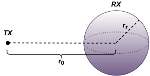
Figure 1: The considered system model of interest.

For the topology presented in Figure 1, denoting the diffusion coefficient of the messenger molecules by $D$, the time density of molecule arrivals (i.e., the channel impulse response, CIR) is presented in [25] to be

$$f_{\textrm{hit}}(t)=\frac{r_{r}}{r_{0}}\frac{1}{\sqrt[]{4\pi Dt}}\frac{r_{0}-r_{r}}{t}e^{-\frac{(r_{0}-r_{r})^{2}}{4Dt}},\hskip 9.95863ptt\in(0,\infty),$$ (1)

with its time integral being equal to

$$F_{\textrm{hit}}(t)=\frac{r_{r}}{r_{0}}\text{erfc}\bigg{(}\frac{r_{0}-r_{r}}{\sqrt[]{4Dt}}\bigg{)}.$$ (2)

Note that Equation (2) represents the probability of a molecule’s arrival at the receiver up to time $t$. In this paper, we consider a time-slotted MCD system where the transmitter and receiver are perfectly synchronized. Using (2), the entries of the channel coefficient vector $\boldsymbol{h}$ can be obtained by

$$h[n]=F_{\textrm{hit}}(nt_{s})-F_{\textrm{hit}}\left((n-1)t_{s}\right),\hskip 14.22636ptn=1,2,\dots,LN,$$ (3)

where $t_{s}$ is the duration of a time slot (sample), $N$ is the number of samples per one symbol duration (i.e., $t_{\textrm{symbol}}=Nt_{s}$), and $L$ denotes the length of the channel memory window in symbols.

Throughout the paper, we consider binary concentration shift keying (BCSK, [4]) signaling with equiprobable symbol transmissions, which defines transmitting a bit-$1$ by emitting $M$ molecules, and a bit-$0$ by emitting no molecules. Note that since BCSK is a binary modulation scheme, the symbol duration is equal to the bit duration ($t_{\textrm{symbol}}=t_{b}$). Herein, we denote $\boldsymbol{s}$ as the binary vector of transmitted bits. Employing BCSK, assuming an idealized transmitter and that the emission occurs at the beginning of the symbol interval, the emission count vector $\boldsymbol{x}$ is given by

$$x[i]=\begin{cases}M,&\text{if $s[k]=1$ and $i=(k-1)N+1$}\\ 0,&\text{otherwise}.\end{cases}$$ (4)

Given the channel coefficient vector $\boldsymbol{h}$ and the emission count vector $\boldsymbol{x}$, the $n^{th}$ sample of the received signal $\boldsymbol{y}$ can be approximated as a Poisson distributed random variable [26]:

$$y[n]\sim\mathcal{P}\left(\lambda_{s}+\sum_{k=1}^{LN}h[k]x[n-k+1]\right),$$ (5)

where $\lambda_{s}$ is the rate of the external Poisson noise. This model is also referred to as the linear time-invariant (LTI)-Poisson channel [27]. Herein, we employ the Gaussian approximation of the Poisson arrival counts [26]. Therefore, for transmissions in blocks of length $S$, and separating the deterministic and random components of $\boldsymbol{y}\sim(\boldsymbol{\mu},\boldsymbol{\Sigma})$, the received signal, in vector form, can be expressed as

$$\begin{split}\boldsymbol{y}=(\boldsymbol{H}\boldsymbol{x}+\lambda_{s}\boldsymbol{j})+\boldsymbol{\eta}.\end{split}$$ (6)

Here, $\boldsymbol{H}$ denotes the $SN\times SN$ Toeplitz matrix corresponding to the convolution operation of LTI-Poisson in (5), $\boldsymbol{j}$ is an $SN\times 1$ vector of ones, and $\boldsymbol{\eta}\sim\mathcal{N}\left(\boldsymbol{0},\boldsymbol{\Sigma}\right)$, where

$$\boldsymbol{\Sigma}=\textrm{diag}\{\boldsymbol{H}\boldsymbol{x}\}+\lambda_{s}\boldsymbol{I}.$$ (7)

Note that $\boldsymbol{\Sigma}$ is dependent on $\boldsymbol{s}$ through $\boldsymbol{x}$, which implies the signal-dependent noise phenomenon of MCD systems [16, 11, 28, 14].

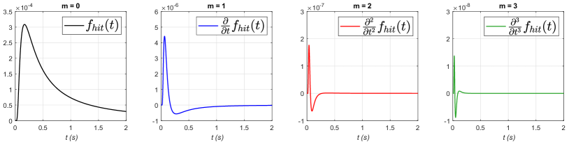
Figure 2: Evolution of $\frac{\partial^{m}f_{hit}}{\partial t^{m}}$ with the derivative order $m$. $r_{0}=$15\text{\,}\mathrm{\SIUnitSymbolMicro m}$$, $r_{r}=$5\text{\,}\mathrm{\SIUnitSymbolMicro m}$$, $D=100\frac{$\text{\,}{\mathrm{\SIUnitSymbolMicro m}}^{2}$}{$\text{\,}\mathrm{s}$}$.

III Fundamentals of Derivative-Based Pre-Processing

Herein, we discuss the main motivation and key statistical properties of the $m^{th}$ order derivative operator in an MCD system. To this end, we first address how the CIR in (1) evolves with the derivative order $m$. Recalling a result from our prior work, the first peak time of $\frac{\partial^{m}f_{\textrm{hit}}}{\partial t^{m}}$ (i.e., the time at which the $m^{th}$ derivative of the CIR achieves its first maximum) is a monotonically decreasing function of the derivative order $m$, [1, Proposition 1]. Furthermore, $\frac{\partial^{m}f_{\textrm{hit}}}{\partial t^{m}}$ shrinks in pulse width with increasing $m$, as clearly observed in Figure 2.

From a receiver design standpoint, the consequence of the above two phenomena is an effective narrowing of each emitted pulse at the receiver, which mitigates ISI for consecutive symbol transmission scenarios. In order to characterize this effect for the time-slotted, discrete time channel, we define the discrete-time forward derivative operator, denoted by $\boldsymbol{D}$, as

$$\boldsymbol{D}=\begin{bmatrix}-1&1&0&\cdots&0\\ 0&-1&1&\cdots&0\\ \vdots&\vdots&\ddots&\ddots&\vdots\\ \vdots&\vdots&&-1&1\\ 0&0&\cdots&0&-1\end{bmatrix}.$$ (8)

Furthermore, we denote the output of the $m^{th}$ order derivative operator as $\boldsymbol{y}_{(m)}\sim\mathcal{N}(\boldsymbol{\mu}_{(m)},\boldsymbol{\Sigma}_{(m)})$. Then, $\boldsymbol{y}_{(m)}$ can be expressed as

$$\begin{split}\boldsymbol{y}_{(m)}&=\boldsymbol{D}^{m}\boldsymbol{y}\\ &=\boldsymbol{D}^{m}\left(\boldsymbol{H}\boldsymbol{x}+\lambda_{s}\boldsymbol{j}\right)+\boldsymbol{D}^{m}\boldsymbol{\eta}\\ &\sim\mathcal{N}\left(\boldsymbol{D}^{m}\boldsymbol{\mu},\boldsymbol{D}^{m}\boldsymbol{\Sigma}(\boldsymbol{D}^{\top})^{m}\right).\end{split}$$ (9)

The mean of $\boldsymbol{y}_{(m)}$ reflects the aforementioned ISI mitigation introduced by the $\boldsymbol{D}^{m}$ operator. However, since $\boldsymbol{\Sigma}_{(m)}=\boldsymbol{D}^{m}\boldsymbol{\Sigma}(\boldsymbol{D}^{\top})^{m}$, the application of the $m^{th}$ order derivative operator inherently introduces noise amplification and coloration into the received signal. We note that the banded diagonal form of $\boldsymbol{D}^{m}$ increases in both width and magnitude with increasing $m$, further increasing the coloration and amplification.

Overall, increasing $m$ results in better ISI mitigation at the cost of a more severe enhancement of the noise power. This interplay between ISI mitigation and noise amplification implies a fundamental trade-off for a derivative-based MCD receiver, implying the existence of an optimal derivative order $m$ that minimizes the error probability. We will address this optimization problem in Section V.

IV Detector Design

Per its description in Section III, the $m^{th}$ order derivative operator can be interpreted as a pre-processor, whose output $\boldsymbol{y}_{(m)}$ is fed to the detector. Through this perspective, Figure 3 presents the overall diagram of an end-to-end MCD system where the receiver employs the $\boldsymbol{D}^{m}$ operator. Herein, we address the design of the detector to be paired with the $m^{th}$ order derivative.

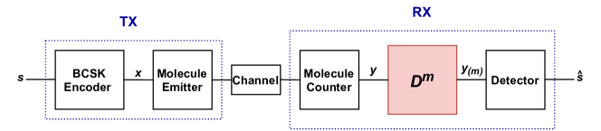
Figure 3: Overall diagram of a derivative pre-processed MCD system.

IV-A Optimal Detector

Our notion of optimality is defined by the maximum-likelihood criterion, which implies that the maximum likelihood sequence detector (MLSD) is optimal due to ISI in the MCD channel [16]. Given that the receiver has access to $\lambda_{s}$ and $\boldsymbol{h}$, the MLSD estimates the transmitted bit sequence $\hat{\boldsymbol{s}}$ using the following rule:

$$\begin{split}\hat{\boldsymbol{s}}&=\operatorname*{arg\,max}_{\boldsymbol{s}}P(\boldsymbol{y}_{(m)}|\boldsymbol{s})\\ &=\operatorname*{arg\,max}_{\boldsymbol{s}}\frac{\exp[-\frac{1}{2}(\boldsymbol{y}_{(m)}-\boldsymbol{\mu}_{(m)})^{T}\boldsymbol{\Sigma}^{-1}_{(m)}(\boldsymbol{y}_{(m)}-\boldsymbol{\mu}_{(m)})]}{{\sqrt{(2\pi)^{SN}|\boldsymbol{\Sigma_{(m)}}|}}}\\ &=\operatorname*{arg\,min}_{\boldsymbol{s}}\Big{\{}\ln(|\boldsymbol{\Sigma}_{(m)}|)+\\ &\hskip 56.9055pt(\boldsymbol{y}_{(m)}-\boldsymbol{\mu}_{(m)})^{T}\boldsymbol{\Sigma}^{-1}_{(m)}(\boldsymbol{y}_{(m)}-\boldsymbol{\mu}_{(m)})\Big{\}}.\end{split}$$ (10)

Here, for each candidate symbol vector $\boldsymbol{s}$, the conditional $\boldsymbol{\mu}_{(m)}$ and $\boldsymbol{\Sigma}_{(m)}$ are found using the corresponding channel statistics presented in Equations (6)-(9). All vectors are of size $SN\times 1$ and the covariance matrix is $SN\times SN$.

IV-B Banded MLSD

The complexity of the MLSD is exponential in channel memory $L$ using the Viterbi algorithm. Unfortunately, as the data rate increases, a shorter bit duration $t_{b}$ implies a larger $L$ due to the heavy tail of the CIR, rendering MLSD infeasible for low-complexity, nano-scale machinery. However, leveraging the aggressive ISI mitigation introduced by the derivative operator, we consider a sub-optimal MLSD-like detector implemented using a considerably shorter memory window $L^{\prime}$. This banded-MLSD approach results in a significantly lower complexity in computation, as it requires $2^{L^{\prime}}$ log-likelihood computations to detect a single symbol, compared to $2^{L}$ required by MLSD ([29, 30]). For this detector, the branch metric $\mathcal{M}(\cdot)$ that is input to the Viterbi decoder has the following form:

$$\begin{split}\mathcal{M}(\boldsymbol{y}^{(i)}_{(m)},\boldsymbol{s}^{(L^{\prime})})&=\ln(|\boldsymbol{\Sigma}^{(L^{\prime})}_{(m)}|)+\\ &\hskip 14.22636pt(\boldsymbol{y}^{(i)}_{(m)}-\boldsymbol{\mu}^{(L^{\prime})}_{(m)})^{\top}{\boldsymbol{\Sigma}^{(L^{\prime})}_{(m)}}^{-1}(\boldsymbol{y}^{(i)}_{(m)}-\boldsymbol{\mu}^{(L^{\prime})}_{(m)}).\end{split}$$ (11)

Here, the superscript $(L^{\prime})$ implies that the vectors and matrices are obtained considering a symbol memory of $L^{\prime}$, and the superscript $(i)$ refers to the samples of the $i^{th}$ symbol. In particular, $\boldsymbol{s}^{(L^{\prime})}$ denotes a candidate symbol string of length $L^{\prime}$. Conditioned on a certain $\boldsymbol{s}^{(L^{\prime})}$, $\boldsymbol{\mu}^{(L^{\prime})}$ and $\boldsymbol{\Sigma}^{(L^{\prime})}$ denote the obtained mean vector and covariance matrix of the samples of the $(L^{\prime})^{th}$ symbol, respectively. Hence, the respective sizes of $\boldsymbol{\mu}^{(L^{\prime})}$ and $\boldsymbol{\Sigma}^{(L^{\prime})}$ are $N\times 1$ and $N\times N$. Furthermore, similar to its conventional use throughout the paper, the subscript $(m)$ implies that the argument vector is pre-multiplied by $\boldsymbol{D}^{m}$, and the argument matrix is pre- and post-multiplied by $\boldsymbol{D}^{m}$ and $(\boldsymbol{D}^{\top})^{m}$, respectively. Note that $\boldsymbol{D}^{m}$ is also of size $N\times N$ herein.

A key observation is that for a fixed derivative order $m$, $y_{(m)}[k]$ is a function of $y[k],\dots,y[k+m]$. Consequently, the $\boldsymbol{D}^{m}$ operator causes the last $m$ samples of the $i^{th}$ symbol to be correlated with the first samples of the $(i+1)^{th}$ symbol, which induces a non-causal ISI. To avoid this issue, we truncate the last $m$ samples of the intended symbol. Hence, $\boldsymbol{\mu}^{L^{\prime}}_{(m)}$ and $\boldsymbol{\Sigma}^{L^{\prime}}_{(m)}$ are of size $(N-m)\times 1$ and $(N-m)\times(N-m)$, respectively. Similarly, noting $\boldsymbol{y}^{(i)}$ corresponds to the arrival counts of the $i^{th}$ symbol, we have $\boldsymbol{y}^{(i)}_{(m)}=\begin{bmatrix}y_{(m)}[(i-1)N+1]&\dots&y_{(m)}[iN-m]\end{bmatrix}^{\top}$.

Assuming standard matrix multiplication, each branch metric computation has cubic complexity in the number of samples per symbol $N$, as the operation involves multiplying vectors and matrices of sizes that are linear in $N$. Note that $\boldsymbol{D}^{m}$ and the conditional vectors/matrices $\boldsymbol{\mu}^{(L^{\prime})}_{(m)}$, $\boldsymbol{\Sigma}^{(L^{\prime})}_{(m)}$, and ${\boldsymbol{\Sigma}^{(L^{\prime})}_{(m)}}^{-1}$ can be pre-computed once and stored, which makes their complexity independent of $N$ and $m$. However, obtaining $\boldsymbol{y}^{(i)}_{(m)}$ from $\boldsymbol{y}^{(i)}$ is not independent of $m$. In particular, although the discrete time forward derivative operation is represented by $\boldsymbol{D}$ for clarity of argument, the operation for obtaining $\boldsymbol{y}^{(i)}_{(m)}$ can be realized with a simple shift register and element-wise subtractions. Therefore, the $m^{th}$ order derivative pre-processor has a complexity of $\mathcal{O}(mN)$ per symbol, making the overall complexity of banded MLSD $\mathcal{O}(m2^{L^{\prime}}N^{3})$.

IV-C Decision Feedback-Aided, Symbol-by-Symbol ML

The banded-MLSD’s complexity is still exponential in $L^{\prime}$, which might be undesirable for a nano-machine. To this end, we generalize the memory limited decision aided decoder (MLDA) proposed in [18] for an arbitrary derivative order $m$, where $m=0$ corresponds to the original version of the detector.

In essence, MLDA is a decision feedback aided, symbol-by-symbol maximum likelihood detector. For each symbol, it first estimates the imposed ISI on the intended symbol’s samples, using the previously decoded symbols. Ideally, the ISI estimation is done using all $L-1$ past decoded symbols. However, due to possible memory or computational constraints of a nano-machine, it might be desirable to consider a shorter memory window of $L^{\prime}$ when estimating the ISI. For this memory-limited case, only $L^{\prime}-1$ past decoded symbols are utilized, and the rest of the past is replaced by the expected transmissions (i.e., using (4) with equiprobable transmissions). The entries of the estimated ISI mean of the $i^{th}$ symbol, denoted by $\hat{\boldsymbol{\mu}}^{(i)}_{\textrm{ISI}}$, is computed according to the previously decoded symbols as follows:

$$\begin{split}\hat{\mu}^{(i)}_{\textrm{ISI}}[n]=&\sum_{k=0}^{(L^{\prime}-1)N-1}h[k+n+1]\hskip 2.84544pt\hat{x}[(i-1)N-k]\\ &+\sum_{k=(L^{\prime}-1)N}^{(L-1)N-1}h[k+n+1]\hskip 2.84544pt\bar{x}[(L-1)N-k],\end{split}$$ (12)

where $\boldsymbol{\hat{x}}$ denotes the decoded emission vector, and is computed through the decoded symbol vector $\boldsymbol{\hat{s}}$ through (4). In addition, $\boldsymbol{\bar{x}}$ denotes the expected transmission vector that covers the past symbols between $(L^{\prime}+1)^{th}$ and $L^{th}$ memory slots, and is expressed as

$$\boldsymbol{\bar{x}}=\begin{bmatrix}\frac{M}{2}&0&\dots&0&\frac{M}{2}&0&\dots\end{bmatrix}^{\top}_{(L-L^{\prime})N\times 1}.$$

After estimating the ISI-induced mean vector, estimated distributions for the samples of possible bit-1 and bit-0 transmissions are computed. Let the estimated (and Gaussian approximated) arrival random vectors be denoted as $\hat{\boldsymbol{y}}^{(i)}_{1}\sim\mathcal{N}(\hat{\boldsymbol{\mu}}^{(i)}_{1},\hat{\boldsymbol{\Sigma}}^{(i)}_{1})$ and $\hat{\boldsymbol{y}}^{(i)}_{0}\sim\mathcal{N}(\hat{\boldsymbol{\mu}}^{(i)}_{0},\hat{\boldsymbol{\Sigma}}^{(i)}_{0})$. The $i^{th}$ sample’s estimated means can be written as

$$\begin{split}\hat{\mu}^{(i)}_{1}[n]&=\hat{\mu}^{(i)}_{\textrm{ISI}}[n]+Mh[n]+\lambda_{s},\\ \hat{\mu}^{(i)}_{0}[n]&=\hat{\mu}^{(i)}_{\textrm{ISI}}[n]+\lambda_{s},\end{split}$$ (13)

where, $\hat{\boldsymbol{\Sigma}}^{(i)}_{j}=\textrm{diag}\{\hat{\boldsymbol{\mu}}^{(i)}_{j}\}$ for $j\in\{0,1\}$, as $\hat{\boldsymbol{y}}^{(i)}_{j}$ are Gaussian approximations of Poisson RVs.

Recalling the truncated arrival vector output of the derivative operator from Subsection IV-B as

$$\boldsymbol{y}^{(i)}_{(m)}=\begin{bmatrix}y_{(m)}[(i-1)N+1]&\dots&y_{(m)}[iN-m]\end{bmatrix}^{\top},$$

the symbol is detected through a likelihood ratio test, that is

$$\hat{s}[i]=\hat{\mathcal{L}}^{(i)}_{(m),1}-\hat{\mathcal{L}}^{(i)}_{(m),0}\mathop{\gtrless}_{0}^{1}0,$$ (14)

where the log-likelihoods are computed as

$$\begin{split}\hat{\mathcal{L}}^{(i)}_{(m),j}=-&\frac{1}{2}\Big{[}(N-m)\ln(2\pi)+\ln(|\hat{\boldsymbol{\Sigma}}^{(i)}_{(m),j})|)+\\ &(\boldsymbol{y}^{(i)}_{(m)}-\hat{\boldsymbol{\mu}}^{(i)}_{(m),j})^{\top}\left(\hat{\boldsymbol{\Sigma}}^{(i)}_{(m),j}\right)^{-1}(\boldsymbol{y}^{(i)}_{(m)}-\hat{\boldsymbol{\mu}}^{(i)}_{(m),j})\Big{]}.\end{split}$$ (15)

Here, $\hat{\boldsymbol{\mu}}^{(i)}_{(m),j}=\boldsymbol{D}^{m}\hat{\boldsymbol{\mu}}^{(i)}_{j}$ and $\hat{\boldsymbol{\Sigma}}^{(i)}_{(m),j}=\boldsymbol{D}^{m}\hat{\boldsymbol{\Sigma}}^{(i)}_{j}(\boldsymbol{D}^{m})^{\top}$.

Overall, MLDA provides a computationally cheaper alternative to banded MLSD, by incurring a linear computational complexity in $L^{\prime}$. Note that for each symbol, evaluating Equations (12)-(13) necessitates holding $(L^{\prime}-1)$ past symbols, and (12) involves the element-wise multiplication of two $(L^{\prime}-1)N$ sample-long vectors. Including the $\mathcal{O}(mN)$ complexity of the $m^{th}$ order differentiation and the $\mathcal{O}(N^{3})$ of (15), the complexity of MLDA is of order $\mathcal{O}(mL^{\prime}N^{3})$.

IV-D Fixed Threshold Detectors

Up to this point, each considered detector employs memory at the receiver side. However, low-complexity and memoryless detectors are particularly desirable for nano-scale applications. To this end, we consider two types of fixed threshold detectors in this subsection. Both detectors rely on comparing the arrival count at a certain sample with a threshold, but they differ in their selection of the arrival count to be compared.

IV-D1 Max-and-Threshold Detector

The max-and-threshold detector (MaTD) selects the sample with the maximum arrival count among the samples corresponding to the intended symbol [20, 1]. The detection steps of the $\boldsymbol{D}^{m}$-MaTD pair can be summarized as follows:

• Employ the derivative operator,

• Discard the last $m$ samples (to cancel non-causal ISI),

• Perform an $\operatorname*{arg\,max}$ operation among the remaining $(N-m)$ samples,

• Compare with the threshold.

In essence, the detected symbol is found by performing

$$\hat{s}[i]=\max\big{(}y_{(m)}[(i-1)N+1],\cdots,y_{(m)}[iN-m]\big{)}\mathop{\gtrless}_{0}^{1}\gamma,$$ (16)

where $\gamma$ is the employed fixed threshold. We note that MaTD with $m=0$ corresponds to the simple asynchronous detector (ADS) proposed in [31].

IV-D2 Fixed Sample, Fixed Threshold Detector

Using MaTD, the sample that observes the maximum number of molecules may differ for each transmitted symbol, as the arrival counts are stochastic. In contrast, as we considered in our prior study [2], the threshold detector can also be realized by fixing the sample whose arrival count is to be compared, yielding the fixed sample, fixed threshold detector (FSTD). In particular, denoting the fixed sample of interest as $\tilde{q}_{(m)}$, FSTD selects $\tilde{q}_{(m)}$ as the “peak sample due to the intended symbol”. In other words, $\tilde{q}_{(m)}$ corresponds to the sample that has the largest expected arrival count due to the intended symbol’s transmission. Let $\boldsymbol{\mu}_{s,(m)}$ denote the expected signal due to the intended symbol after the $m^{th}$ order derivative operator is applied at the receiver. We note that since the peak of $\boldsymbol{\mu}_{s,(m)}$ changes with $m$ (see Figure 2), $\tilde{q}_{(m)}$ is a function of $m$. Overall, the $\boldsymbol{\mu}_{s,(m)}$ vector can be expressed as

$$\boldsymbol{\mu}_{s,(m)}=\boldsymbol{D}^{m}\boldsymbol{\mu}_{s},$$ (17)

where

$$\boldsymbol{\mu}_{s}=\begin{cases}\begin{bmatrix}Mh[1]&\dots&Mh[N]\end{bmatrix}^{\top},&\text{if bit-$1$}\\ \begin{bmatrix}0&\dots&0\end{bmatrix}^{\top},&\text{if bit-$0$}.\end{cases}$$ (18)

Similar to previously discussed strategies, for a derivative order of $m$, the last $m$ samples of $\boldsymbol{\mu}_{s,(m)}$ are again discarded to avoid non-causal ISI. Following this truncation, and denoting $\boldsymbol{\bar{\mu}}_{s,(m)}$ as the expected $\boldsymbol{\mu}_{s,(m)}$, FSTD selects $\tilde{q}_{(m)}$ by performing

$$\tilde{q}_{(m)}=\operatorname*{arg\,max}_{q\in\{1,\dots,N-m\}}\hskip 8.5359pt\left|\bar{\mu}_{s,(m)}[q]\right|.$$ (19)

The maximization in (19) does not perform the $\operatorname*{arg\,max}$ operation on $\boldsymbol{\mu}_{s,(m)}$ itself, but selects the sample with the largest signal in the absolute sense. Note that due to the nature of time differentiation and the $f_{hit}(t)$ function, $\boldsymbol{\mu}_{s,(m)}$ can have both positive and negative elements (see Figure 2). In some cases, the smallest negative element can actually have a larger absolute value than the largest positive element, implying that said negative sample is larger in energy. In such a case, FSTD simply negates the received signal and finds $\tilde{q}_{(m)}$ using the negated signal. Overall, the decision rule for FSTD can be expressed as

$$\hat{s}[i]=\begin{cases}y_{(m)}[(i-1)N+\tilde{q}_{(m)}]\mathop{\gtrless}_{0}^{1}\gamma,&\textrm{if}\hskip 4.26773pt{\mu}_{s,(m)}[\tilde{q}_{(m)}]\geq 0\\ -y_{(m)}[(i-1)N+\tilde{q}_{(m)}]\mathop{\gtrless}_{0}^{1}\gamma,&\textrm{if}\hskip 4.26773pt{\mu}_{s,(m)}[\tilde{q}_{(m)}]<0.\end{cases}$$ (20)

We note that FSTD is a generalization of the fixed sample, fixed threshold detector that is widely used in the MCD literature ([32, 33, 34]) to an arbitrary derivative order $m$, where $m=0$ corresponds to the original version of the detector.

Since both MaTD and FSTD are memoryless detectors, their complexities for decoding a symbol do not depend on a memory window length $L^{\prime}$. For FSTD, as the threshold comparison is done using a fixed sample, the complexity does not depend on $N$ either. For MaTD, finding the maximum on $N-m$ samples has linear complexity in $N$. Overall, combining with the $\mathcal{O}(mN)$ of the derivative pre-processing, both MaTD and FSTD have complexities of order $\mathcal{O}(mN)$. This result suggests the conjunction of $\boldsymbol{D}^{m}$ and fixed threshold detectors are particularly useful for low complexity, nano- to micro-scale applications. Motivated by this, we will mainly consider fixed threshold detectors throughout the rest of the paper, with a particular focus of FSTD for the problem of derivative order optimization. In the numerical results, Section VI, we will compare performance of all of the detectors discussed herein.

V The Optimization of $m$

V-A Error Probability Analysis

With the derivative order $m$ as a design parameter, the question of how to optimize it arises. Herein, we address this derivative order optimization problem for fixed threshold detectors. As the end goal is to minimize the error rate of the transmission, we first derive the theoretical bit error probability of the $\boldsymbol{D}^{m}$-FSTD pair.

Recalling that the considered MCD channel is an ISI channel with memory length $L$, the theoretical error probability expression will average over all $(L-1)$ symbol-long strings of data. Denoting $\boldsymbol{s}_{\textrm{ISI}}$ as the $(L-1)$ symbol-long vector that holds said string, the error probability can be found by performing

$$P_{e}=\frac{1}{2^{L-1}}\big{(}\sum_{\forall\boldsymbol{s}_{\textrm{ISI}}}P_{e|\boldsymbol{s}_{\textrm{ISI}}}\big{)}.$$ (21)

Conditioned on a certain symbol vector $\boldsymbol{s}_{L}=\begin{bmatrix}\boldsymbol{s}_{\textrm{ISI}}&s[L]\end{bmatrix}^{\top}$, the received signal mean can be written as

$$\begin{split}\boldsymbol{\mu}_{L}&=E(\boldsymbol{y}_{L}|\boldsymbol{x}_{L})\\ &=\boldsymbol{H}_{L}\boldsymbol{x}_{L}+\lambda_{s}\boldsymbol{j}_{N},\end{split}$$ (22)

where $\boldsymbol{j}_{N}$ is an $N$ sample-long vector of ones, the received vector $\boldsymbol{y}_{L}=\begin{bmatrix}y[(L-1)N+1]&\cdots&y[LN]\end{bmatrix}^{T}$, $\boldsymbol{x}_{L}$ is the corresponding $LN$ sample-long transmission vector corresponding to $\boldsymbol{s}_{L}$ through (4), and

$$\boldsymbol{H}_{L}=\begin{bmatrix}h[(L-1)N+1]&\cdots&h[1]&0&\cdots&0\\ \vdots&\cdots&&\ddots&\ddots&\vdots\\ h[LN-1]&\cdots&&h[2]&h[1]&0\\ h[LN]&\cdots&&h[3]&h[2]&h[1]\end{bmatrix}.$$ (23)

Similar to (7), the covariance matrix is then found by $\boldsymbol{\Sigma}_{L}=\textrm{diag}\{\boldsymbol{\mu}_{L}\}$. Therefore, after applying the $m^{th}$ order derivative operator, the mean vector and covariance matrix associated with each conditional becomes $\boldsymbol{\mu}_{L,(m)}=\boldsymbol{D}^{m}\boldsymbol{\mu}_{L}$ and $\boldsymbol{\Sigma}_{L,(m)}=\boldsymbol{D}^{m}\boldsymbol{\Sigma}_{L}(\boldsymbol{D}^{\top})^{m}$, respectively.

Using these conditional statistics, we are interested in finding $P_{e|\boldsymbol{s}_{\textrm{ISI}}}$, which can be expressed for FSTD as

$$\begin{split}P_{e|\boldsymbol{s}_{\textrm{ISI}}}=&\frac{1}{2}\big{(}P(B\hskip 1.42271pty_{(m)}[(L-1)N+\tilde{q}_{(m)}]<\gamma|s_{L}[L]=1)\\ &+P(B\hskip 1.42271pty_{(m)}[(L-1)N+\tilde{q}_{(m)}]>\gamma|s_{L}[L]=0)\big{)}\\ =&\frac{1}{2}(A_{1}+A_{0}),\end{split}$$ (24)

where $\tilde{q}_{(m)}$ is the fixed sample found by Equations (18)-(19), and $B=\operatorname{sgn}\left(\mu_{s,(m)}[\tilde{q}_{(m)}]\right)$ with $\operatorname{sgn}(\cdot)$ defining the signum function. As we employ the Gaussian approximation of the Poisson arrivals, (24) can be re-written as

$$\begin{split}A_{1}=Q\Big{(}\frac{B\hskip 1.42271pt\mu_{L,(m)}[\tilde{q}_{(m)}]-\gamma}{\sqrt{\Sigma_{L,(m)}[\tilde{q}_{(m)},\tilde{q}_{(m)}]}}\Big{|}s_{L}[L]=1\Big{)}\\ A_{0}=Q\Big{(}\frac{\gamma-B\hskip 1.42271pt\mu_{L,(m)}[\tilde{q}_{(m)}]}{\sqrt{\Sigma_{L,(m)}[\tilde{q}_{(m)},\tilde{q}_{(m)}]}}\Big{|}s_{L}[L]=0\Big{)},\end{split}$$ (25)

where $Q(\cdot)$ is the Gaussian $Q$-function, which concludes the derivation. Note that $A_{1}$ and $A_{0}$ consider the same $\boldsymbol{s}_{\textrm{ISI}}$. However, they differ in $s_{L}[L]$, hence the mean vectors and covariance matrices presented in (25) are not equal.

Error Analysis of the $\boldsymbol{D}^{m}$-MaTD Pair: As noted in Subsection IV-D, we focus on FSTD as the primary threshold-based detector in this paper. However, we also provide the error probability derivation of the $\boldsymbol{D}^{m}$-MaTD pair, as it may be more desirable in scenarios where the receiver is not capable of locating the expected signal peak location for FSTD.

Similar to FSTD, due to the ISI nature of the MCD channel, the error probability of $\boldsymbol{D}^{m}$-MaTD is also found by averaging over the conditional error probabilities. Similarly, the computation of conditional statistics is also not dependent on the detector strategy. Therefore, Equations (21)-(23) hold for the $\boldsymbol{D}^{m}$-MaTD pair as well.

The derivation for the $\boldsymbol{D}^{m}$-MaTD pair differs from that of the $\boldsymbol{D}^{m}$-FSTD pair in the way it computes the conditional error probabilities. To evaluate a conditional error probability for the $\boldsymbol{D}^{m}$-MaTD pair, we first denote

$$Y_{(m)}=\underset{j\in\{1,\dots,N-m\}}{\max}\hskip 1.42271pty_{L,(m)}[j]$$

as the maximum sample. Then, $P_{e|\boldsymbol{s}_{\textrm{ISI}}}$ can be expressed as

$$\begin{split}P_{e|\boldsymbol{s}_{\textrm{ISI}}}&=\frac{1}{2}\big{(}P(Y_{(m)}<\gamma|s_{L}[L]=1)+P(Y_{(m)}>\gamma|s_{L}[L]=0)\big{)}\\ &=\frac{1}{2}(A^{\prime}_{1}+A^{\prime}_{0})\end{split}$$ (26)

Therefore, characterizing the CDF of $Y_{(m)}$ is sufficient to complete the derivation. However, $Y_{(m)}$ corresponds to the maximum of correlated and differently distributed Gaussian random variables, for which a straightforward, closed form solution does not appear to exist. Instead, numerical solutions are typically considered [35, 36]. Motivated by this, we use the strategy developed by Clark [37] to approximate $Y_{(m)}$ as a normal random variable through a recursive process. We refer the reader to Appendix A for the details of the recursion. At the end of the Clark’s approximation process, we obtain the approximate Gaussian distribution $Y_{(m)}\sim\mathcal{N}(\mu_{R},\sigma^{2}_{R})$. We plug these statistics into (26) as

$$\begin{split}A^{\prime}_{1}=Q\Big{(}\frac{\mu_{R}-\gamma}{\sigma_{R}}\Big{|}s_{L}[L]=1\Big{)}\\ A^{\prime}_{0}=Q\Big{(}\frac{\gamma-\mu_{R}}{\sigma_{R}}\Big{|}s_{L}[L]=0\Big{)},\end{split}$$ (27)

which completes the derivation.

V-B Signal-to-Interference-Plus-Noise Ratio

Due to the presence of the $2^{L-1}$ conditional error probabilities which constitute the theoretical BER, optimizing the BER resulting from a particular choice of $m$ is computationally infeasible given the typical values of $L$ associated with an MCD channel. In particular, even though our earlier study suggested considering $L^{\prime}<L$ to decrease this complexity [1], our observations suggest that such a simplification can lose accuracy for very high data rate settings, even with the aggressive right tail mitigation of the $\boldsymbol{D}^{m}$ operator. Furthermore, as for the case of true $L$, we still need to compute multiple $Q$-functions for $L^{\prime}$ as well (Equation (25)), which may be undesirable for a simple nano-machine.

Motivated by the aforementioned shortcomings of optimizing $m$ by examining the theoretical error probabilities, we generalize the signal-to-interference-plus-noise ratio (SINR) employed by [28] to the $\boldsymbol{D}^{m}$-FSTD pair. Overall, for an arbitrary symbol index $k$, the expression has the following form [2]:

$$\operatorname{SINR}(m) =\frac{E\left\{\left(s[k]\mu_{s,(m)}[\tilde{q}_{(m)}]\right)^{2}\right\}}{\operatorname{Var}\left\{\eta_{(m)}^{(k)}[\tilde{q}_{(m)}]\right\}+\operatorname{Var}\left\{\mathcal{I}_{(m)}^{(k)}[\tilde{q}_{(m)}]\right\}},$$ (28)

where the superscript $(k)$ indicates that the symbol of interest is the $k^{th}$. In the sequel, we characterize each term in the expression. Firstly, the numerator corresponds to the second moment of the signal that is induced by the intended symbol’s ($k^{th}$) transmission. Recalling the definition of $\boldsymbol{\mu}_{s,(m)}$ from (17) and that $\tilde{q}_{(m)}$ is $\boldsymbol{D}^{m}$-FSTD’s sample of interest, the numerator is expressed as

$$\begin{split}E\left\{\left(s[k]\mu_{s,(m)}[\tilde{q}_{(m)}]\right)^{2}\right\}&=\frac{1}{2}\times 0+\frac{1}{2}E\left\{\left(\mu_{s,(m)}[\tilde{q}_{(m)}]\right)^{2}\right\}\\ &=\frac{1}{2}\left(\mu_{s,(m)}[\tilde{q}_{(m)}]\right)^{2}.\end{split}$$ (29)

In the denominator, the first expression represents the noise variance induced by the intended symbol’s transmission. Let $\boldsymbol{\Sigma}_{s}=\operatorname{diag}(\boldsymbol{\mu}_{s})$ and $\boldsymbol{\Sigma}_{s,(m)}=\boldsymbol{D}^{m}\boldsymbol{\Sigma}_{s}(\boldsymbol{D}^{m})^{\top}$. Then, the noise variance incurred by the intended symbol is expressed as

$$\begin{split}\operatorname{Var}\left\{\eta_{(m)}^{(k)}[\tilde{q}]\right\}&=\frac{1}{2}\operatorname{Var}\left\{\eta_{(m)}^{(k)}[\tilde{q}]\Big{|}s[k]=0\right\}+\\ &\hskip 56.9055pt\frac{1}{2}\operatorname{Var}\left\{\eta_{(m)}^{(k)}[\tilde{q}]\Big{|}s[k]=1\right\}\\ &=\frac{1}{2}\times 0+\frac{1}{2}\boldsymbol{\Sigma}_{s,(m)}[\tilde{q}_{(m)},\tilde{q}_{(m)}]\\ &=\frac{1}{2}\left\{\boldsymbol{D}^{m}\operatorname{diag}(\boldsymbol{\mu}_{s})(\boldsymbol{D}^{m})^{\top}\right\}[\tilde{q}_{(m)},\tilde{q}_{(m)}].\end{split}$$ (30)

Lastly, characterizing the noise variance induced by ISI and external noise completes the derivation of (28). To this end, we first denote $\boldsymbol{\mu_{I}}$ as the mean arrival count vector that is due to ISI. Note that $\boldsymbol{\mu_{I}}$ depends on the evaluated ISI symbol sequence $\boldsymbol{s}_{\textrm{ISI}}$. We then define

$$\begin{split}\boldsymbol{\mu}_{I,(m)}&=\boldsymbol{D}^{m}\left(\boldsymbol{\mu_{I}}+\lambda_{s}\boldsymbol{j}\right)\\ \boldsymbol{\Sigma}_{I,(m)}&=\boldsymbol{D}^{m}\operatorname{diag}(\boldsymbol{\mu_{I}}+\lambda_{s}\boldsymbol{j})(\boldsymbol{D}^{\top})^{m}.\end{split}$$ (31)

Overall, the variance induced by ISI and external noise can be found by

$$\begin{split}\operatorname{Var}&\left\{\mathcal{I}_{(m)}^{(k)}[\tilde{q}_{(m)}]\right\}=\operatorname{Cov}(y_{(m)}^{(k)}[\tilde{q}_{(m)}],y_{(m)}^{(k)}[\tilde{q}_{(m)}])\\ &=E\left[\left(y_{(m)}^{(k)}[\tilde{q}_{(m)}]\right)^{2}\right]-\left(E\left[y_{(m)}^{(k)}[\tilde{q}_{(m)}]\right]\right)^{2}\\ &=E_{\boldsymbol{s}_{ISI}}\left[\left(y_{(m)}^{(k)}[\tilde{q}_{(m)}]\right)^{2}\Big{|}\boldsymbol{s}_{ISI}\right]-\\ &\hskip 99.58464pt\left(E_{\boldsymbol{s}_{ISI}}\left[y_{(m)}^{(k)}[\tilde{q}_{(m)}\big{|}\boldsymbol{s}_{ISI}]\right]\right)^{2}\\ &=\frac{1}{2^{L-1}}\sum_{\forall\boldsymbol{s}_{ISI}}\left[\boldsymbol{\Sigma}_{I,(m)}[\tilde{q}_{(m)},\tilde{q}_{(m)}]+\left(\mu_{I,(m)}[\tilde{q}_{(m)}]\right)^{2}\right]-\\ &\hskip 99.58464pt\left(\frac{1}{2^{L-1}}\sum_{\forall\boldsymbol{s}_{ISI}}\mu_{I,(m)}[\tilde{q}_{(m)}]\right)^{2}.\end{split}$$ (32)

Similar to the theoretical BER expressions, evaluating SINR also incurs an exponential complexity in $L$ stemming from computing conditional statistics when evaluating (32). To avoid this, one can use a smaller memory window of $L^{\prime}<L$ when evaluating SINR, significantly reducing the incurred complexity. Denoting this version of SINR as $\operatorname{SINR}_{L^{\prime}}$, the objective function presented in this subsection can be used to select the derivative order as follows:

$$m^{*}=\operatorname*{arg\,max}_{m}\hskip 4.26773pt\operatorname{SINR}_{L^{\prime}}(m).$$ (33)

VI Numerical Results

In this section, we present numerical results to assess the accuracies of the theoretical error probability expressions derived in Subsection V-A, demonstrate the efficacy of SINR as an objective function for optimizing $m$, and provide comparative BER results for derivative/no-derivative detectors. Throughout the section, the external Poisson noise rate ($\lambda_{s}$) is normalized with respect to transmission power through the following definition of signal-to-noise ratio (SNR):

$$\textrm{SNR}=\frac{\frac{M}{2}}{N\lambda_{s}}=\frac{M}{2N\lambda_{s}}.$$ (34)

Here, the numerator follows from (4) for equiprobable BCSK symbols, and represents the average emitted signal per one symbol. Recalling $N$ as the number of samples per one symbol duration and $\lambda_{s}$ as the external noise rate per symbol, the denominator of (34) represents the expected number of external noise molecules per one symbol.

Since parameters such as $D$, $r_{r}$, and $r_{0}$ all affect the $f_{hit}(t)$ function hence the $\boldsymbol{h}$ vector. To this end, in order to contextualize the data rate in relation to these parameters, we normalize the symbol duration with respect to the channel peak time $t_{p}=\frac{d^{2}}{6D}=\frac{(r_{0}-r_{r})^{2}}{6D}$, see [25, Equation 26]. Throughout this section, the bit duration $t_{b}$ is selected through a unitless parameter $S_{r}$, which is defined as $S_{r}=\frac{t_{b}}{t_{p}}$. Note that since a smaller $t_{b}$ corresponds to a higher rate of transmission, a smaller $S_{r}$ corresponds to a higher data rate.

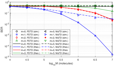
(a) $S_{r}=0.5$.

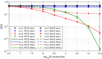
(b) $S_{r}=0.25$.

Figure 4: Theoretical and simulated BER vs. $M$. $\textrm{SNR}=10$dB, $r_{0}=$15\text{\,}\mathrm{\SIUnitSymbolMicro m}$$, $r_{r}=$5\text{\,}\mathrm{\SIUnitSymbolMicro m}$$, $D=$100\text{\,}{\mathrm{\SIUnitSymbolMicro m}}^{2}\text{\,}{\mathrm{s}}^{-1}$$, $N=5$, $L=10$. $\gamma$ values numerically optimized through exhaustive search.

VI-A Accuracy of Error Analysis

Herein, we demonstrate the accuracy of the derived theoretical BER expressions for $\boldsymbol{D}^{m}$-FSTD and $\boldsymbol{D}^{m}$-MaTD pairs with varying $m$. To this end, Figures 4a and 4b are presented for different values of $S_{r}$ (hence, different data rates). In both figures, $L=10$ is selected for demonstrative purposes, due to the exponential complexity when computing the theoretical BER expressions.

The results of Figures 4a and 4b show that the theoretical BER expression for $\boldsymbol{D}^{m}$-FSTD is accurate, and the approximations for $\boldsymbol{D}^{m}$-MaTD are tight. Furthermore, confirming the results of [2], FSTD is found to generally outperform MaTD. Motivated by this, among the fixed threshold detectors, we will present the error curves for $\boldsymbol{D}^{m}$-FSTD throughout this section. Lastly, regardless of the comparative relationship between FSTD and MaTD, it can be observed that both detectors benefit from the derivative operator and produce lower BER values with $m>0$ compared to their standard versions with $m=0$.

VI-B Accuracy of SINR

In this subsection, we show the accuracy of the SINR expression derived in Subsection V-B. To this end, we provide Figures 5a-5b and Figures 5c-5d to present results for two different data rates, and thus, two different levels of ISI. Similar to the theoretical error probability expressions, the SINR also necessitates evaluating over $2^{L-1}$ ISI symbol sequences. For computational complexity reasons, we use the limited memory, $\operatorname{SINR}_{L^{\prime}}$ version of the expression with $L^{\prime}=10$. However, we note that the BER simulations use large channel memories ($L=100$ for Figure 5b and $L=200$ for Figure 5d) to satisfactorily capture the right tail of the CIR, and to test the memory-limited SINR’s efficacy in the more accurate large channel memory scenario.

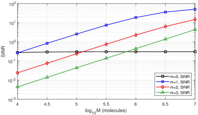
(a) SINR vs. $M$, $S_{r}=0.5$, $L^{\prime}=10$.

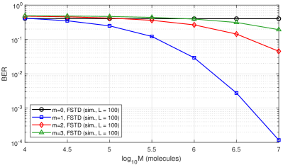
(b) Theoretical and Simulated BER vs. $M$, $S_{r}=0.5$, $L=100$.

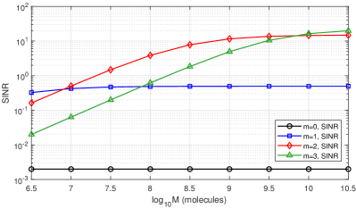
(c) SINR vs. $M$, $S_{r}=0.25$, $L^{\prime}=10$.

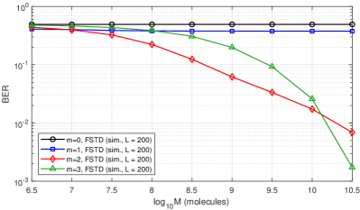
(d) Theoretical and Simulated BER vs. $M$, $S_{r}=0.25$, $L=200$.

Figure 5: BER and SINR vs. $M$. $\textrm{SNR}=10$dB, $r_{0}=$15\text{\,}\mathrm{\SIUnitSymbolMicro m}$$, $r_{r}=$5\text{\,}\mathrm{\SIUnitSymbolMicro m}$$, $D=$100\text{\,}{\mathrm{\SIUnitSymbolMicro m}}^{2}\text{\,}{\mathrm{s}}^{-1}$$, $N=5$. $\gamma$ values numerically optimized through exhaustive search.

The results of Figure 5 demonstrate that SINR closely follows the comparative trend between different derivative orders. Furthermore, SINR provides this accuracy with a significantly smaller memory consideration than the true channel memory, which suggests its utility for derivative order optimization in micro- to nano-scale applications. That said, SINR can incur slight discrepancies in the comparative trend when the BER values of evaluated schemes are close. An example of this phenomenon can be observed in Figures 5c-5d, between $m=2$ and $3$ at $M=10^{10}$ molecules. The discrepancy is due to the substantially smaller memory used to compute the SINR. We refer the reader to compare Figures 5c and 4b, which are with $L=L^{\prime}=10$, to confirm SINR’s accuracy when the considered memories are equal.

The comparative trends between different orders of $m$ in Figures 5b and 5d show that, as theorized and predicted, the optimal derivative order is a function of system parameters. In particular, Figure 5b shows that for a relatively smaller $S_{r}$ (hence lower ISI) a smaller $m$ is better. On the other hand, Figure 5d shows that in a larger $S_{r}$/higher ISI regime, higher derivative orders outperform the first order. These results can be explained through the fundamental trade-off between ISI mitigation and noise amplification associated with the $\boldsymbol{D}^{m}$ operator. Recall from Section III and Figure 2 that a higher derivative order induces a lower ISI due to a narrower effective pulse duration, at a cost of an increase in received signal variance. In light of this trade-off, the results of Figure 5b show that for lower ISI, the system is better off by avoiding the additional noise amplification of $m>1$ as the ISI is already relatively low. However, the higher data rate in Figure 5d incurs a very high level of ISI, which induces the need for a more aggressive ISI mitigation, causing the optimal $m$ to be larger than one. Another noteworthy trend in Figure 5d is that the optimal derivative order changes with $M$. Figure 5d shows that in the small $M$ regime, $m=2$ is optimal. However, as $M$ increases, the system is able to combat the noise amplification better, hence is able to leverage the more powerful ISI mitigation provided by $m=3$.

VI-C Asymptotic Performance

In the previous subsection, we discussed the implications of the ISI mitigation-noise amplification trade-off of the derivative pre-processor. In particular, we noted that for low ISI and/or small $M$ scenarios, a smaller $m$ is better due to less noise amplification. On the other hand, in general, as $M$ increases, the system becomes more robust against noise, and is better-off by increasing the derivative order for better ISI mitigation. From these two trends, the following question might arise: As $M\rightarrow\infty$, do the performances of derivative orders become monotonically better as $m$ increases? To this end, although BER vs. $M$ curves cannot be provided due to extremely low error rates, we leverage the accuracy of SINR in explaining the comparative relationship of different derivative orders for $\boldsymbol{D}^{m}$-FSTD, and provide SINR vs. $M$ curves in Figure 6.

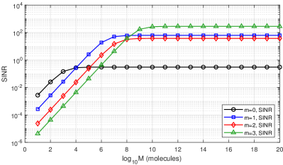
(a) $S_{r}=0.5$.

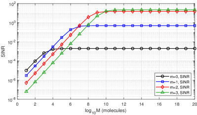
(b) $S_{r}=0.25$.

Figure 6: SINR vs. $M$. $\textrm{SNR}=10$dB, $r_{0}=$15\text{\,}\mathrm{\SIUnitSymbolMicro m}$$, $r_{r}=$5\text{\,}\mathrm{\SIUnitSymbolMicro m}$$, $D=$100\text{\,}{\mathrm{\SIUnitSymbolMicro m}}^{2}\text{\,}{\mathrm{s}}^{-1}$$, $N=5$, $L^{\prime}=10$.

As expected, the results of Figure 6b show that the SINR is monotonically decreasing in $m$ at the small $M$ regime, whereas for asymptotically large $M$, the SINR is monotonically increasing. Our empirical observations with various channel and system parameters verify that this trend is typical, confirming the implications of the ISI mitigation-noise amplification trade-off. However, Figure 6a exemplifies that it is not always the case. We return to the sampling argument for Equation (19). In the context of (19), we had noted that time differentiation causes some samples of the derivative pre-processed signal to have large negative amplitudes in expectation. In addition to this, for some scenarios, the same effect of time differentiation can also cause the samples to more evenly share the total received power within a symbol duration. In such cases, the maximum sample considered by FSTD has a smaller absolute magnitude, making the system face a higher error floor due to ISI. The computation of SINR implicitly accounts for this phenomenon and predicts the comparative relationships for asymptotically large $M$.

VI-D BER vs. Detector Memory

We next consider the effects of detector memory in error performance for the banded MLSD and MLDA. Figure 7 presents BER versus $L^{\prime}$. For benchmarking purposes, Figure 7 also includes the results for minimum mean squared error (MMSE) equalizer. We note that the MMSE, when applied on the transmission block as a whole, has complexity that is quadratic in block length $S$, which is undesirable for a simple nano-machine. Hence, following the consideration of [16], we employ the decision feedback-aided, online version of the MMSE equalizer herein (which is $\mathcal{O}(L^{\prime 2}N^{2})$ for the emission strategy considered in Equation (4)).

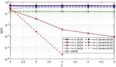
Figure 7: BER vs. $L^{\prime}$. $S_{r}=0.25$, $\log_{10}M=8.5$ molecules, $\textrm{SNR}=10$dB, $r_{0}=$15\text{\,}\mathrm{\SIUnitSymbolMicro m}$$, $r_{r}=$5\text{\,}\mathrm{\SIUnitSymbolMicro m}$$, $D=$100\text{\,}{\mathrm{\SIUnitSymbolMicro m}}^{2}\text{\,}{\mathrm{s}}^{-1}$$, $N=5$, $L=200$.

Figure 7 demonstrates three noteworthy trends:

1. Derivative-based pre-processing allows for a reduction in the memory window of memory-aided detectors, courtesy of its ISI mitigating nature. We emphasize that even though the true channel memories are on the order of hundreds of symbols, reliable communication can be achieved using a substantially smaller $L^{\prime}$. Combined with the very low complexity nature of the discrete-time derivative operation itself, the combination of the pre-processor and detector remain low complexity, providing high-performance, computationally cheap MCD receivers amenable to micro- and nano-scale MCD applications.

2. The ISI mitigation-noise amplification trade-off affects the optimal derivative order in memory-aided detectors as well. However, in memory-aided detectors, the optimal derivative order is also affected by the choice of $L^{\prime}$. To exemplify, we note that the stronger ISI mitigation of $m=3$ makes the schemes with $m=3$ outperform other orders at $L^{\prime}=2$. On the other hand, the schemes with $m=2$ provide lower error rates for $L^{\prime}\geq 3$ due to less noise amplification.

3. Due to its very definition, as $L^{\prime}\rightarrow L$, the performance of the banded MLSD would converge to the MLSD Viterbi decoder. For the same derivative order, the results of Figure 7 show that banded MLSD typically outperforms its MLDA counterpart in the small $L^{\prime}$ regime as well. That said, we note that MLDA is also capable of yielding a reliable error performance at this regime, and is a low complexity alternative to banded MLSD therein. Overall, we conclude that $\boldsymbol{D}^{m}$-banded MLSD is able to provide a lower BER with higher complexity, and vice versa for $\boldsymbol{D}^{m}$-MLDA, confirming the performance-complexity trade-off between them.

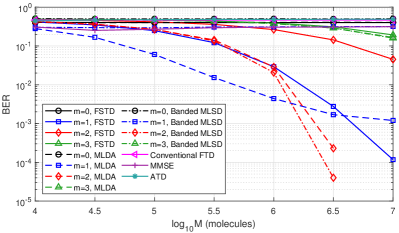
(a) BER vs. $M$, $S_{r}=0.5$, $L=100$.

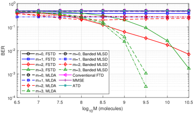
(b) BER vs. $M$, $S_{r}=0.25$, $L=200$.

Figure 8: BER vs. $M$. $\textrm{SNR}=10$dB, $r_{0}=$15\text{\,}\mathrm{\SIUnitSymbolMicro m}$$, $r_{r}=$5\text{\,}\mathrm{\SIUnitSymbolMicro m}$$, $D=$100\text{\,}{\mathrm{\SIUnitSymbolMicro m}}^{2}\text{\,}{\mathrm{s}}^{-1}$$, $N=5$, $L^{\prime}=2$. $\gamma$ values numerically optimized through exhaustive search.

VI-E Comparative Error Performance

In this subsection, we provide the comparative error performances of the proposed strategies through Figure 8. We note that due to their comparable computational complexities, Figure 8 also includes the conventional fixed threshold detector (FTD, [4]) where the total arrival count within a symbol duration is compared with a threshold, and the adaptive threshold detector (ATD) proposed in [17]. Moreover, in order to ensure a relatively comparable complexity to FSTD, the memory aided detectors/equalizers are implemented with $L^{\prime}=2$.

The results of Figure 8 agree with the previously presented results regarding the benefits of the derivative operator. Among the derivative-based schemes, for the majority of the evaluated data points in Figure 8, either $\boldsymbol{D}^{m}$-banded MLSD or $\boldsymbol{D}^{m}$-MLDA are observed to outperform other schemes. That said, $\boldsymbol{D}^{m}$-FSTD is also found to provide reliable error rates despite its simplicity. Comparing the strategies on a target BER level, it can be inferred that $\boldsymbol{D}^{m}$-banded MLSD and $\boldsymbol{D}^{m}$-MLDA are able to reach the target with a smaller $M$ than $\boldsymbol{D}^{m}$-FSTD, whereas $\boldsymbol{D}^{m}$-FSTD offers a lower receiver complexity at a cost of increased transmission power.

VII Conclusions

In this paper, receiver-side higher order time differentiation has been proposed to mitigate ISI for MCD. Considering the derivative operation as a pre-processor block before detection, several memory-aided (i.e., MLSD, banded MLSD, MLDA) and memoryless (i.e., FSTD, MaTD) detectors have been provided to be paired with the derivative operator. In the paper, it is shown that for a derivative-based MCD receiver, there exists a fundamental trade-off between ISI mitigation and noise amplification, implying the existence of an optimal derivative order that minimizes BER. The derivative order optimization problem is addressed for fixed threshold detectors, through the derivations of the theoretical BER expressions of $\boldsymbol{D}^{m}$-FSTD and $\boldsymbol{D}^{m}$-MaTD pairs. Furthermore, an SINR-like objective function is proposed to optimize $m$ for $\boldsymbol{D}^{m}$-FSTD. Numerical results confirm the accuracy of the derived expressions, demonstrate the efficacy of the $\boldsymbol{D}^{m}$ operator in ISI mitigation, and show that said ISI mitigation decreases the needed memory window of memory-aided detectors. Overall, the proposed $\boldsymbol{D}^{m}$ operator is shown to be a computationally very cheap strategy that provides a powerful ISI mitigation. Given the transmitter is able to handle large transmission powers to alleviate the effects of noise amplification, the derivative operator allows for achieving considerably higher data rates, while still preserving a reliable communication link.

Appendix A Clark’s Approximation for MaTD

Let $X_{i}=y_{L,(m)}[i]$ where $\boldsymbol{y}_{L,(m)}=\boldsymbol{D}^{m}\boldsymbol{y}_{L}$. Then, $X_{1},\dots,X_{N-m}$ are correlated and differently distributed random variables whose maximum’s distribution is of interest. In its first iteration, Clark’s approximation finds the mean and the variance of $\max(X_{1},X_{2})$. Afterwards, $\max(X_{1},X_{2})$ is approximated as a Gaussian with said mean and variance. Then, in the second iteration, $\max(X_{1},X_{2},X_{3})=\max[\max(X_{1},X_{2}),X_{3}]$ simply becomes the maximum of two “Gaussians”, which is handled in a similar way to the first iteration. The process keeps iterating until the $n^{th}$ random variable.

Herein, we present the method of finding the mean and the variance of $\max(X_{1},X_{2})$. Let $X_{1}\sim\mathcal{N}(\mu_{1},\sigma^{2}_{1})$ and $X_{2}\sim\mathcal{N}(\mu_{2},\sigma^{2}_{2})$. Note that by definition, $\mu_{i}$ is the $i^{th}$ entry of $\boldsymbol{\mu}_{L,(m)}$, and $\sigma^{2}_{i}$ is the $i^{th}$ diagonal entry of $\boldsymbol{\Sigma}_{L,(m)}$. We define two auxiliary parameters $a$ and $\alpha$ to be

$$\begin{split}a&=\sqrt{\sigma^{2}_{1}+\sigma_{2}^{2}-2\sigma_{1,2}}\\ \alpha&=\frac{\mu_{1}-\mu_{2}}{a}.\end{split}$$ (35)

Let $\nu_{1}$ and $\nu_{2}$ denote the first and second moments of $\max(X_{1},X_{2})$. Then,

$$\begin{split}\nu_{1}&=\mu_{1}Q(-\alpha)+\mu_{2}Q(\alpha)+a\psi(\alpha)\\ \nu_{2}&=(\mu^{2}_{1}+\sigma^{2}_{1})Q(-\alpha)+(\mu^{2}_{2}+\sigma^{2}_{2})Q(\alpha)+(\mu_{1}+\mu_{2})a\psi(\alpha),\end{split}$$ (36)

where $\psi(\cdot)$ denotes the standard normal PDF. Lastly, using $\nu_{1}$ and $\nu_{2}$, we approximate $\max(X_{1},X_{2})\sim\mathcal{N}(\nu_{1},\nu_{2}-\nu^{2}_{1})$, completing the iteration.

References

- [1] M. C. Gursoy and U. Mitra, “Higher order derivatives: Improved pre-processing and receivers for molecular communications,” in IEEE Global Communications Conference (GLOBECOM), Dec. 2020, pp. 1–6.
- [2] ——, “On the optimization of derivative-based receivers for molecular communications,” in Proc. ACM International Conference on Nanoscale Computing and Communication (ACM NanoCom), Sept. 2021.
- [3] T. Suda, M. Moore, T. Nakano, R. Egashira, A. Enomoto, S. Hiyama, and Y. Moritani, “Exploratory research on molecular communication between nanomachines,” in Genet. Evol. Comput. Conf. (GECCO), Jun. 2005, pp. 25–29.
- [4] M. S. Kuran, H. B. Yilmaz, T. Tugcu, and I. F. Akyildiz, “Modulation techniques for communication via diffusion in nanonetworks,” in Proc. IEEE International Conference on Communications (ICC), Apr. 2011, pp. 1–5.
- [5] N.-R. Kim and C.-B. Chae, “Novel modulation techniques using isomers as messenger molecules for nano communication networks via diffusion,” IEEE Journal on Selected Areas in Communications, vol. 31, no. 12, pp. 847–856, Jan. 2013.
- [6] N. Garralda, I. Llatser, A. Cabellos-Aparicio, E. Alarcón, and M. Pierobon, “Diffusion-based physical channel identification in molecular nanonetworks,” Nano Commun. Netw., vol. 2, no. 4, pp. 196–204, Dec. 2011.
- [7] M. C. Gursoy, E. Basar, A. E. Pusane, and T. Tugcu, “Index modulation for molecular communication via diffusion systems,” IEEE Trans. Commun., vol. 67, no. 5, pp. 3337–3350, May 2019.
- [8] Y. Huang, M. Wen, L.-L. Yang, C.-B. Chae, and F. Ji, “Spatial modulation for molecular communication,” IEEE Transactions on NanoBioscience, vol. 18, no. 3, pp. 381–395, Jul. 2019.
- [9] H. Arjmandi, A. Gohari, M. N. Kenari, and F. Bateni, “Diffusion-based nanonetworking: A new modulation technique and performance analysis,” IEEE Communications Letters, vol. 17, no. 4, pp. 645–648, Mar. 2013.
- [10] M. C. Gursoy, D. Seo, and U. Mitra, “A concentration-time hybrid modulation scheme for molecular communications,” IEEE Transactions on Molecular, Biological, and Multi-Scale Communications, pp. 1–1, 2021.
- [11] R. Mosayebi, A. Gohari, M. Mirmohseni, and M. Nasiri-Kenari, “Type-based sign modulation and its application for ISI mitigation in molecular communication,” IEEE Transactions on Communications, vol. 66, no. 1, pp. 180–193, Jan. 2018.
- [12] T. Nakano, A. W. Eckford, and T. Haraguchi, Molecular Communication. Cambridge University Press, 2013.
- [13] M. S. Kuran, H. B. Yilmaz, I. Demirkol, N. Farsad, and A. Goldsmith, “A survey on modulation techniques in molecular communication via diffusion,” IEEE Communications Surveys and Tutorials, vol. 23, no. 1, pp. 7–28, 2021.
- [14] M. C. Gursoy, M. Nasiri-Kenari, and U. Mitra, “Towards high data-rate diffusive molecular communications: Performance enhancement strategies,” arXiv preprint arXiv:2101.02869, Jan. 2021.
- [15] B. Tepekule, A. E. Pusane, M. S. Kuran, and T. Tugcu, “A novel pre-equalization method for molecular communication via diffusion in nanonetworks,” IEEE Communications Letters, vol. 19, no. 8, pp. 1311–1314, Jun. 2015.
- [16] D. Kilinc and O. B. Akan, “Receiver design for molecular communication,” IEEE Journal on Selected Areas in Communications, vol. 31, no. 12, pp. 705–714, Dec. 2013.
- [17] M. Damrath and P. A. Hoeher, “Low-complexity adaptive threshold detection for molecular communication,” IEEE Transactions on NanoBioscience, vol. 15, no. 3, pp. 200–208, 2016.
- [18] R. Mosayebi, H. Arjmandi, A. Gohari, M. Nasiri-Kenari, and U. Mitra, “Receivers for diffusion-based molecular communication: Exploiting memory and sampling rate,” IEEE Journal on Selected Areas in Communications, vol. 32, no. 12, pp. 2368–2380, Dec. 2014.
- [19] T.-Y. Tung and U. Mitra, “Synchronization error robust transceivers for molecular communication,” IEEE Transactions Molecular, Biological, and Multi-Scale Communications, vol. 5, no. 3, pp. 207–221, Dec. 2019.
- [20] H. Yan, G. Chang, Z. Ma, and L. Lin, “Derivative-based signal detection for high data rate molecular communication system,” IEEE Communications Letters., vol. 22, no. 9, pp. 1782–1785, Sep. 2018.
- [21] Y. Huang, X. Chen, M. Wen, L.-L. Yang, C.-B. Chae, and F. Ji, “A rising edge-based detection algorithm for MIMO molecular communication,” IEEE Wireless Communications Letters, vol. 9, no. 4, pp. 523–527, Apr. 2020.
- [22] J. Adler, “Chemotaxis in bacteria,” Science, vol. 153, no. 3737, pp. 708–716, Aug. 1966.
- [23] F. Arsène, T. Tomoyasu, and B. Bukau, “The heat shock response of escherichia coli,” International Journal of Food Microbiology, vol. 55, no. 1, pp. 3–9, Apr. 2000.
- [24] J.-P. Huertas, A. Aznar, A. Esnoz, P. S. Fernández, A. Iguaz, P. M. Periago, and A. Palop, “High heating rates affect greatly the inactivation rate of escherichia coli,” Frontiers in microbiology, vol. 7, p. 1256, Aug. 2016.
- [25] H. B. Yilmaz, A. C. Heren, T. Tugcu, and C.-B. Chae, “Three-dimensional channel characteristics for molecular communications with an absorbing receiver,” IEEE Communications Letters., vol. 18, no. 6, pp. 929–932, Jun. 2014.
- [26] H. B. Yilmaz and C.-B. Chae, “Arrival modelling for molecular communication via diffusion,” IET Electronics Letters, vol. 50, no. 23, pp. 1667–1669, Nov. 2014.
- [27] G. Aminian, H. Arjmandi, A. Gohari, M. Nasiri-Kenari, and U. Mitra, “Capacity of diffusion-based molecular communication networks over LTI-Poisson channels,” IEEE Transactions on Molecular, Biological, and Multi-Scale Communications, vol. 1, no. 2, pp. 188–201, Nov. 2015.
- [28] V. Jamali, A. Ahmadzadeh, and R. Schober, “On the design of matched filters for molecule counting receivers,” IEEE Communications Letters, vol. 21, no. 8, pp. 1711–1714, May 2017.
- [29] G. D. Forney, “The Viterbi algorithm,” Proc. IEEE, vol. 61, no. 3, pp. 268–278, 1973.
- [30] A. Kavcic and J. M. F. Moura, “The Viterbi algorithm and Markov noise memory,” IEEE Trans. Info. Theory, vol. 46, no. 1, pp. 291–301, 2000.
- [31] A. Noel and A. W. Eckford, “Asynchronous peak detection for demodulation in molecular communication,” in Proc. IEEE International Conference on Communications (ICC). IEEE, May 2017, pp. 1–6.
- [32] L.-S. Meng, P.-C. Yeh, K.-C. Chen, and I. F. Akyildiz, “On receiver design for diffusion-based molecular communication,” IEEE Transactions on Signal Processing, vol. 62, no. 22, pp. 6032–6044, Nov. 2014.
- [33] A. Noel, K. C. Cheung, and R. Schober, “Improving receiver performance of diffusive molecular communication with enzymes,” IEEE Transactions on NanoBioscience, vol. 13, no. 1, pp. 31–43, 2014.
- [34] I. Llatser, A. Cabellos-Aparicio, M. Pierobon, and E. Alarcon, “Detection techniques for diffusion-based molecular communication,” IEEE Journal on Selected Areas in Communications, vol. 31, no. 12, pp. 726–734, Dec. 2013.
- [35] J. Blanchet and C. Li, “Efficient simulation for the maximum of infinite horizon discrete-time gaussian processes,” Journal of Applied Probability, vol. 48, no. 2, p. 467–489, 2011.
- [36] Z. I. Botev, M. Mandjes, and A. Ridder, “Tail distribution of the maximum of correlated gaussian random variables,” in Proc. Winter Simulation Conference, Dec. 2015, pp. 633–642.
- [37] C. E. Clark, “The greatest of a finite set of random variables,” Operations Research, vol. 9, no. 2, pp. 145–162, 1961.
- [38] W. R. Greer Jr. and G. J. La Cava, “Normal approximations for the greater of two normal random variables,” Omega, vol. 7, no. 4, pp. 361–363, 1979.