The Supernova Remnant Populations of the galaxies NGC 45, NGC 55, NGC 1313, NGC 7793: Luminosity and Excitation Functions.

Abstract

We present a systematic study of the Supernova Remnant (SNR) populations in the nearby galaxies NGC 45, NGC 55, NGC 1313, and NGC 7793 based on deep H$\rm{\alpha}$ and [S ii] imaging. We find 42 candidate and 54 possible candidate SNRs based on the [S ii]/H$\rm{\alpha}$>0.4 criterion, 84 of which are new identifications. We derive the H$\rm{\alpha}$ and the joint [S ii]-H$\rm{\alpha}$ luminosity functions after accounting for incompleteness effects. We find that the H$\rm{\alpha}$ luminosity function of the overall sample is described with a skewed Gaussian with a mean equal to $\rm\log(L_{H\alpha}/10^{36}\,erg\,s^{-1})=0.07$ and $\rm\sigma(\log(L_{H\alpha}/10^{36}\,erg\,s^{-1}))=0.58$. The joint [S ii]-H$\rm{\alpha}$ function is parameterized by a skewed Gaussian along the log([S ii]$\rm/10^{36}\,erg\,s^{-1})=0.88\times\log(L_{H\alpha}/10^{36}\,erg\,s^{-1})-0.06$ line and a truncated Gaussian with $\rm\mu(\log(L_{[S\,II]}/10^{36}))=0.024$ and $\rm\sigma(\log(L_{[S\,II]}/10^{36}))=0.14$, on its vertical direction. We also define the excitation function as the number density of SNRs as a function of their [S ii]/H$\rm{\alpha}$ ratios. This function is represented by a truncated Gaussian with a mean at -0.014. We find a sub-linear [S ii]-H$\rm{\alpha}$ relation indicating lower excitation for the more luminous objects.

1 Introduction

Supernova remnants (SNRs) are an integral component of the interstellar medium (ISM) of a galaxy. These sources drive the evolution of the ISM through the deposition of large amounts of chemically-enriched material and kinetic energy. They are related to the star-forming process within a galaxy, since under appropriate conditions, their shock waves compress the ISM, triggering new-star formation. In addition, core-collapse SNRs are tracers of the on-going massive star formation since they are the last stage in the life of massive stars ($\rm{M>8\,M\odot}$; Condon & Yin 1990).

In our Galaxy, 294 SNRs have been identified so far, based on the systematic study in radio bands (Green 2019). Many of them have been studied in various wavelengths (e.g. Milisavljevic & Fesen 2013; Boumis et al. 2009; Slane et al. 2002) yielding detailed information on their physical and morphological properties, as well as their interaction with their local ISM. Studying SNRs in different wavelengths gives us the opportunity to examine different gas phases of SNRs, from gases with temperatures ranging from thousands to millions of degrees and through different evolutionary stages. However, the study of Galactic SNRs has some disadvantages: optical and X-ray bands are suffering from significant extinction, leading sometimes to incomplete samples. In addition, the study of Galactic SNRs does not allow us to examine SNR populations that evolve in a wide range of ISM parameters (e.g. different density distributions, metallicities). Another important limitation of studies in Galactic SNRs is that it is very difficult to estimate their distances. The study of extragalactic SNRs remedies these limitations. They give us the opportunity to explore larger and more diverse samples that can be correlated to different ISM and galaxy properties. In addition, extragalactic sources overcome the problems of Galactic absorption and distance uncertainties, since they are considered to be at the distance of their host galaxy. Taking advantage of these benefits, many studies of SNRs in nearby galaxies have been carried out (e.g. Long et al. 2019; Lee & Lee 2015; Leonidaki, Boumis, & Zezas 2013; Leonidaki, Zezas, & Boumis 2010; Blair & Long 1997; Matonick & Fesen 1997; Lacey & Duric 1997; Pannuti et al. 2000; Pannuti, Schlegel, & Lacey 2007). These studies increase the number of known SNRs and thus provide significant information on their nature not only on individual objects, but also on their overall population and their effect on their host galaxy.

A significant limitation of these surveys is that they do not account for the effect of incompleteness. During the detection process, there is a fraction of SNRs that we do not detect because of their faintness, the detection process, and the method we have followed for the selection and identification of SNRs. These effects make our samples incomplete. Incompleteness is a fundamental problem that can affect significantly our results. For example, we can see features in luminosity functions which are not real and they are simply artefacts of the detection and selection process. This problem is exacerbated by the commonly used practice of SNR identification based on visual inspection of $\rm H\alpha$, [S ii], and [S ii]/$\rm H\alpha$ maps. Visual inspection, being a subjective method, does not allow the reliable quantification of the selection effects. The effect of incompleteness does not allow us to exploit the full extent of the available data. This is particularly important for studying the low luminosity end of the SNR population and hence obtaining a more complete picture of their population and their feedback to ISM.

In this work, we present a systematic study of SNRs in 4 nearby galaxies: NGC 45, NGC 55, NGC 1313, and NGC 7793. We present a new way for the detection and characterization of the SNR population that bypasses the commonly used practice of visual inspection. This has the advantage of allowing the calculation of incompleteness, which in turn, enables the derivation of luminosity functions and more reliable statistics on the SNR populations. We do not restrict this analysis only to H$\rm{\alpha}$ luminosity but we also construct the joint incompleteness-corrected luminosity functions (LFs) for H$\rm{\alpha}$ and [S ii], the two parameters that we use for the detection. This has the additional benefit of allowing the simultaneous calculation of the SNR excitation (i.e. the [S ii]/H$\rm\alpha$ ratio) as a function of the H$\rm{\alpha}$ luminosity.

In Section 2, we describe the sample of the galaxies and their characteristics. In Section 3 and Section 4 we present the observations, the data reduction, the detection of SNRs and the photometric analysis. We also describe how we calculate the incompleteness corrections. The luminosity function and the excitation as a function of the H$\rm{\alpha}$ luminosity are presented in Section 5 and in Section 6 we discuss our results in the context of extragalactic SNR populations. In Section 7 we summarize our results.

2 Sample

Our sample consists of four southern galaxies: NGC 45, NGC 55, NGC 1313, and NGC 7793. Their basic properties are given in Table 1. The main selection criteria for our sample are: (1) They are nearby galaxies, (D<7 Mpc) allowing identification of individual objects; (2) They are face on in order to minimize the effects of internal extinction (only NGC 55 is edge-on but its extinction is very low); (3) They are all spiral galaxies. (4) They have available X-ray data from the Chandra X-ray observatory (the total exposure time of the Chandra data is presented in Table 1).

They also have similar metallicities, limiting metallicity effects in the characterization of SNRs. The [O/H] metallicities given in Table 1, are calculated using the [N ii]$\rm\lambda\lambda 6548,6583$/H$\rm{\alpha}$ line ratios from the work of Kennicutt et al. (2008), which were converted to metallicities using the ($\rm 12+log(O/H)=8.9+0.59log([\text{N\,{ii}}]/H\alpha)$) calibration of Pettini & Pagel (2004). The extinction corrected H$\rm\alpha$ star formation rate (SFR) that is presented in Table 1, has been obtained by Lee et al. (2009).

This work supplements our previous multi-wavelength study of SNRs in nearby galaxies, which showed evidence for differences in SNRs between spiral and irregular galaxies. More specifically, it is seen that more luminous X-ray emitting SNRs tend to be preferentially associated with irregular galaxies (see Fig.12 of Leonidaki, Zezas, & Boumis 2010) which is attributed to different ISM density between the two types of galaxies.

Table 1: Galaxies Properties.

Galaxy	Distance∗	Size∗∗	RA	Dec	Metallicity	SFR(H$\rm\alpha$)	Chandra data
			(J2000)	(J2000)
	(Mpc)	(arcmin)	hh:mm:ss	dd:mm:ss		$\rm{M_{\odot}\,yr^{-1}}$	total exposure time∗∗∗ (ks)
NGC 45	6.79	8.5, 5.9	00:14:03.99	-23:10:55.5	8.51	0.39	65.06
NGC 55	1.99	32.4, 5.6	00:14:53.60	-39:11:47.9	8.54	0.47	68.93
NGC 1313	4.15	9.1, 6.9	03:18:16.05	-66:29:53.7	8.62	0.67	68.98
NGC 7793	3.70	9.3, 6.3	23:57:49.83	-32:35:27.7	8.54	0.51	2190.26

• Col (1): The name of the galaxies; col (2) the distance of the galaxies; col (3) the size of the galaxies; col (4) and col (5): the Right Ascension and Declination of the galaxies; col (6): the $\rm{[12+log(O/H)]}$ metallicity of the galaxies; col (7): the extinction corrected H$\rm\alpha$ SFR. (Lee et al. 2009).
  ^∗The distance and the size characteristics are taken from the NED (NASA/IPAC Extragalactic Database; http://ned.ipac.caltech.edu/).
  ^∗∗Major and minor axis.
  ^∗∗∗ The exposure time does not include observations in sub-array mode.

All four galaxies are known to host SNRs identified in optical, radio, or X-ray wavelengths. However, the available studies are not systematic, not allowing the investigation of their populations in detail. From our sample, only NGC 7793 has been studied in optical wavelengths. Blair & Long (1997) detected and spectroscopically confirmed 27 SNRs, with H$\rm\alpha$ fluxes ranging from $\rm 6.7\times 10^{-16}$ to $\rm 3.6\times 10^{-14}\,erg\,cm^{-2}\,s^{-1}$. Two of them have been also confirmed by Della Bruna et al. (2020). Pannuti et al. (2011, 2002) presented 7 radio SNRs, 2 of which coincide with optical SNRs, while the rest of them are new identification. More recently, Galvin et al. (2014) presented a catalogue of 14 radio SNRs that includes 5 of the 7 aforementioned radio SNRs. Two of them coincide with optical SNRs from the work of Blair & Long (1997).

Dodorico, Dopita, & Benvenuti (1980) looked for optical SNRs in NGC 45 but without any success. However, a candidate SNR in radio with no X-ray counterpart and a candidate one in X-rays are reported in the work of Pannuti et al. (2015). NGC 55 has given 6 radio candidate SNRs that are reported to have also X-ray emission (O’Brien et al. 2013). Five SNRs have been detected in the X-ray band (Stobbart, Roberts, & Warwick 2006) and 2 of them have also emission in radio (Hummel et al. 1986). In addition, 13 more X-ray SNRs have been reported in the study of Binder et al. (2015). In NGC 1313, a probable young SNR around the supernova SN 1978K has been identified in the X-rays (Smith et al. 2007, Colbert et al. 1995; Schlegel, Petre, & Colbert 1996; Petre et al. 1994) and in radio (Achterberg & Ball 1994). Colbert et al. (1995) presents also 4 probable SNRs in X-rays.

Table 2: Observation details

Filters	RA	Dec	Exposure Time	Exposures	PSF	Date
	(J2000)	(J2000)	(sec)		(arcsec∗)
NGC 45
H$\rm{\alpha}$ + [N ii]	00:14:03.48	-23:10:56.20	3600	5 $\times$ 720$\rm s$	0.95	17 Nov 2011
[S ii]	00:14:04.11	-23:10:37.80	7200	5 $\times$ 1440$\rm s$	1.30	17 Nov 2011
R	00:14:05.10	-23:10:07.70	600	5 $\times$ 120$\rm s$	1.30	17 Nov 2011
NGC 55
H$\rm{\alpha}$ + [N ii]	00:14:53.95	-39:11:46.39	3600	5 $\times$ 720$\rm s$	1.03	16 Nov 2011
[S ii]	00:14:53.53	-39:11:47.60	7200	5 $\times$ 1440$\rm s$	1.22	16 Nov 2011
R	00:14:53.67	-39:11:48.50	600	5 $\times$ 120$\rm s$	1.32	16 Nov 2011
NGC 1313
H$\rm{\alpha}$ + [N ii]	03:18:16.75	-66:29:52.00	3600	5 $\times$ 720$\rm s$	0.95	15 Nov 2011
[S ii]	03:18:17.60	-66:29:54.49	5760	4 $\times$ 1440$\rm s$	1.30	16 Nov 2011
R	03:18:16.01	-66:29:53.99	600	5 $\times$ 120$\rm s$	0.92	15 Nov 2011
NGC 7793
H$\rm{\alpha}$ + [N ii]	23:57:49.82	-32:35:28.10	3600	5 $\times$ 720$\rm s$	0.95	15 Nov 2011
[S ii]	23:57:49.83	-32:35:28.20	7200	5 $\times$ 1440$\rm s$	0.97	15 Nov 2011
R	23:57:49.78	-32:35:28.20	600	5 $\times$ 120$\rm s$	1.05	15 Nov 2011

• Col (1): The filters that were used; col (2) and col (3): the RA and Dec of each exposure; col (4) the exposure time: col (5): the number of the exposures; col (6): the PSF of the obtained images; col (7): the date of each observation.
  ^∗ It is the FWHM of the PSF.

3 Observations and Data reduction

The data used in this work were obtained with the 4-m Blanco telescope at CTIO (Chile) on November 15-17, 2011. We used the $36\arcmin\times 36\arcmin$ Mosaic II CCD imager which consists of 8 CCDs ($2048\times 2048$ SITe each) with a pixel scale of $0.27\arcsec/\rm{pixel}$. We used the narrow band H$\rm{\alpha}$ + [N ii] and [S ii] filters and a broadband continuum R filter. For the H$\rm{\alpha}$ + [N ii] filter, the central wavelength is 6563Å with a FWHM of 80 Å, for the [S ii] filter the central wavelength is 6725 Å with a FWHM of 80 Å, and for the R continuum, the central wavelength is 6440 Å with a FWHM of 1510 Å.

The total exposure time for each galaxy was 3600 sec for the H$\rm{\alpha}$ + [N ii], 7200 for the [S ii], and 600 sec for the R-continuum filters. The integration time for each observation was split into 5 shorter exposures. For the larger galaxies, the pointing for each of the 5 observations was shifted slightly to cover the chip gaps. This dither procedure ensures uniform coverage of the galaxy and efficient removal of cosmic rays. Detailed information on the observations for each galaxy is given on Table 2.

For the reduction of the mosaic images, we used the mscred package of IRAF (Image Reduction and Analysis Facility; Tody 1993, 1986). Bias and flat-field corrections were performed on all images; astrometric calibrations were applied on the reduced CCD images using the 2MASS catalog and a fourth order polynomial to account for distortions at the edges of the images. The individual exposures for each object and each filter were registered and median combined with SWarp

4 Detection and Photometry

The first step in our analysis was the detection of discrete sources in each galaxy. To do this, we used the program SExtractor (Bertin & Arnouts 1996). SExractor was chosen because in comparison to similar tools, it is more effective in the detection of fainter objects located in dense star fields, as well as spatially varying backgrounds, with significant structure (Annunziatella et al. 2013). We ran SExtractor setting the following parameters for the H$\rm\alpha$ + [S ii] image: a) detection threshold at 2.5$\rm\sigma$ above the background, b) the minimum number of source pixels equal to 5, and c) the background mesh size at 5 pixels in order to account for small-scale background variations. From the detected sources in each image, we kept only those within the optical outline of the galaxy in H$\rm\alpha$. This region is defined as the region for which the intensity in H$\rm\alpha$ is 3$\sigma$ above the background.

The next step was the photometric analysis of the sources which was performed using the package phot of IRAF. The intensity of the detected sources was measured by means of a curve of growth analysis (i.e. we measure the source intensity in apertures of increasing radius and adopting the one maximising the signal to noise ratio). The optimal aperture radius for the majority of sources is 4.0 pixels corresponding to 35.2 pc, 10.3 pc, 21.5 pc, and 19.2 pc, for NGC 45, NGC 55, NGC 1313, and NGC 7793 respectively.

In order to subtract the star-light continuum from the detected sources, for each galaxy we selected stars of moderate intensity and for each of them we calculated the intensity ratios $\rm{(H\alpha+[\text{N\,{ii}}])/R}$ and $\rm{[\text{S\,{ii}}]/R}$ where H$\rm{\alpha}$, [S ii], and R are the measured intensities in the H$\alpha$, [S ii] and R-continuum images respectively. The mode of these ratios was used as a scaling factor for the R-continuum intensity before subtracting it from the measured H$\rm{\alpha+[\text{N\,{ii}}]}$ and [S ii] intensities.

An additional correction needed to obtain the net H$\rm\alpha$ flux is to subtract the contribution of the [N ii]$\rm\lambda\lambda$6548,6584Å  lines . We adopted a $\rm{([\text{N\,{ii}}]\lambda\lambda 6548,6584)/H\alpha}$ flux ratio of 0.27, based on emission-line measurements of spectroscopically identified SNRs of galaxies with similar metallicities of our sample (Long et al. 2018, Leonidaki, Boumis, & Zezas 2013, Blair & Long 1997).

To examine possible contamination by H ii regions resulting from over-subtraction of the [N ii] contamination, we considered the spectroscopic [N ii]/H$\rm\alpha$ ratio of H ii regions in NGC 1232 (Lima-Costa et al. 2020), NGC 300 and NGC 7793 (Blair & Long 1997), NGC 7793 (Bibby & Crowther 2010), M31 (Zurita & Bresolin 2012) and M33 (Lin et al. 2017). From the average values of the ratios reported in each of those works, the lowest is 0.19. We find that by adopting the ratio [N ii]/H$\rm\alpha$ = 0.27 there are $\sim$ 29% more H ii regions (for [S ii]/H$\rm\alpha$ ratio 3$\rm\sigma$ above the 0.4 threshold) than when we consider the ratio [N ii]/H$\rm\alpha$ = 0.19 for the H ii regions. This is a rather conservative fraction since we consider the lowest [N ii]/H$\rm\alpha$ ratio of the H ii region sample (the mean value of the [N ii]/H$\rm\alpha$ ratio of the rest of the studies ranges from 0.2-0.38). In general, it is very difficult to have zero contamination by H ii regions in an SNR photometric sample, especially because the contamination by [N ii] in the H$\rm\alpha$ flux cannot be predicted exactly for each source. However, a spectroscopic SNR sample can also suffer from contamination by H ii regions because there are H ii regions that may have [S ii]/H$\rm\alpha$ > 0.4. This can be alleviated by using diagnostics that combine more line ratios (Kopsacheili, Zezas, & Leonidaki 2020).

In order to flux calibrate the detected sources, we used observations of standard stars from the catalogue of Massey et al (1988). We obtained photometry for these stars at different airmasses and we performed a linear fit of their instrumental magnitude against the airmass $\rm\chi$: $\rm{m=m_{inst}-k\chi+b}$ where $\rm m$ is the calibrated magnitude, and $\rm k$ and $\rm b$ the slope and the intercept that are to be calculated. Hence we have:

      $\rm{m_{v}=-2.5log(f_{\nu})-48.9=-2.5log(count\,rate)-kx+b}$

where $\nu$ is the central frequency of the filter that we use. Finally, in order to convert flux density to flux, we also multiply with the FWHM (Full Width at Half Maximum) of the filter.

At this point, we have the continuum subtracted H$\rm{\alpha}$ and [S ii] flux of every detected source. In order to find which of them are SNRs, we followed a totally automated method. From the full sample of sources, we first consider those with H$\rm{\alpha}$ flux above the 3$\rm{\sigma}$ level with respect to the local background. Then, the SNRs are identified by applying the standard [S ii]/H$\rm{\alpha}$ > 0.4 criterion (Mathewson & Clarke 1973), considering sources with [S ii]/H$\rm{\alpha}$ > 0.4 at the 3$\rm{\sigma}$ level (candidate SNRs) and at the 2$\rm{\sigma}$ (possible candidate SNRs). To ensure the reliability of the sources identified in this automated way, we visually inspected each one of them, on the H$\rm{\alpha}$, [S ii], and R images. This showed that some of them found to be parts of larger structures, for example rings, large bubbles and filaments. These extended sources are not considered for further analysis. All other candidate SNRs are reliable identifications, based on their appearance on the [S ii] and H$\rm\alpha$ images, ensuring the reliability of the automated method.

4.1 Calculation of Incompleteness

During the detection process, a fraction of the sources is not detected due to their faintness in combination to their environment and stochastic effects. For this reason, our sample (as any observational sample) is characterized by incompleteness which depends on the H$\rm{\alpha}$ local background, the detection method, and sample selection effects. In order to evaluate this incompleteness, we followed the standard approach of placing artificial objects on our images (with the IRAF task addstar) using their measured PSF (determined with the IRAF package PSF) and in a wide range of magnitudes, covering the full brightness range of the observed objects in each filter.

Then we perform the detection exactly as we did for the actual data. The process of adding and recovering artificial sources is repeated multiple times to improve our statistics. In every iteration we took special care to include at most as many artificial sources as objects observed in the actual data, in order to avoid increasing the source confusion. Then, we performed aperture photometry on the artificial objects, the same way as in the actual data, keeping only the sources that are 3$\rm{\sigma}$ above the background in H$\rm{\alpha}$, then the sources with [S ii]/H$\rm{\alpha}$ > 0.4, and finally the sources for which the ratio is 3$\rm{\sigma}$ above 0.4. This results in three samples: an H$\rm{\alpha}$ sample, a [S ii]/H$\rm{\alpha}$ selected sample, and a "secure" [S ii]/H$\rm{\alpha}$ sample ([S ii]/H$\rm{\alpha}$ > 0.4 at 3$\rm{\sigma}$ significance).

In order to create a 2D incompleteness map, we divide the input artificial star magnitude range of the (H$\rm\alpha$, S ii) plane, in 2 dimensional bins, and we calculate the fraction of input and detected objects (after applying all relevant selection criteria) for each ($\rm L_{H\alpha},L_{[S\,II]}$) bin. This comparison is performed on the continuum-subtracted fluxes: the continuum subtraction is achieved by subtracting the R-band continuum flux using the same scaling factor as for the real data, since the artificial objects are placed on the same background as the actual data. So now, we have the fraction of detected/input objects (incompleteness) as a function of their H$\rm{\alpha}$ and [S ii] intensities.

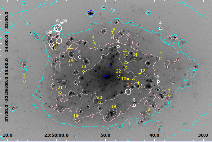
Because of the varying diffuse emission surface brightness, the incompleteness varies within each galaxy. To account for this variation, we calculate the incompleteness for four different background regimes for each galaxy. These are selected to trace the full range of backgrounds in which sources are detected in each galaxy. Indicatively, in Figure 4 we show the different regions with contours for NGC 7793.

In order to estimate the false positives (the sources that have been measured to have [S ii]/H$\rm{\alpha}$ > 0.4 at the 3$\rm\sigma$ level while in reality they do not), from the initial artificial objects we created two sub-samples, one for sources with input [S ii]/H$\rm{\alpha}$ ratio between 0.2 and 0.3, and one for input ratio between 0.3 and 0.4. Then, we examined what fraction of sources detected with ratio > 0.4 belongs to these two sub-samples.

5 Results

5.1 Candidate SNRs

In total, we detected 42 candidate SNRs (with [S ii]/H$\rm{\alpha}$ ratio 3$\rm{\sigma}$ above the 0.4 threshold, 30 of which are new identifications) and 54 new possible candidate SNRs (with [S ii]/H$\rm{\alpha}$ ratio 2$\rm{\sigma}$ above the 0.4 threshold). In addition, some of the knots that present high excitation ([S ii]/H$\rm{\alpha}$ > 0.4), in both 3$\rm{\sigma}$ and 2$\rm{\sigma}$ samples, are part of larger structures (i.e shells, bubbles etc, with sizes from $\sim$ 40 pc $-$ $\sim$ 320 pc). In total, we identify 21 such structures, with those with small radii (i.e. $<$ 100 pc) probably being SNRs. These objects are not considered in our candidate SNR samples, but they are reported for completeness and follow-up observations.

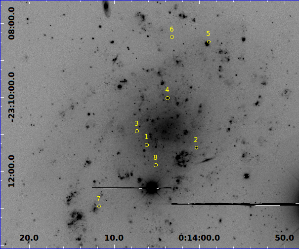
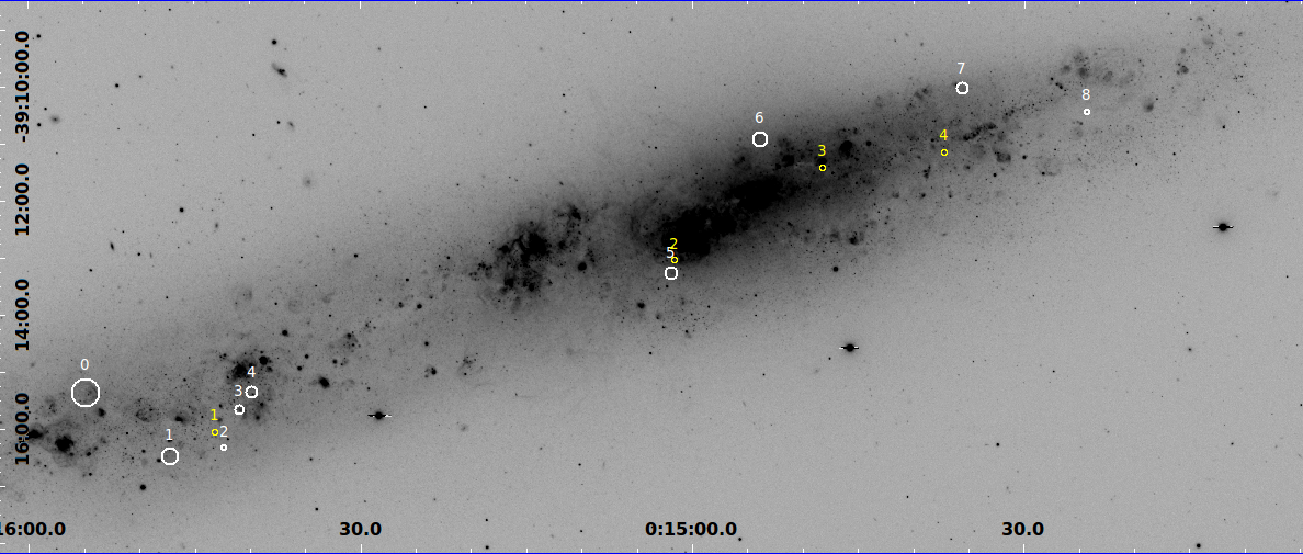
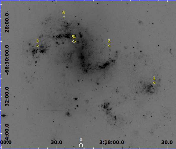
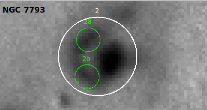
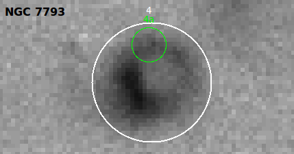
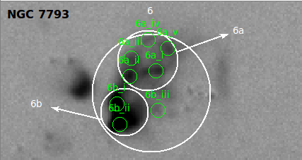
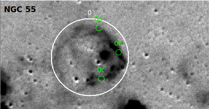
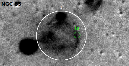
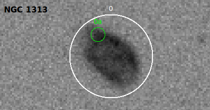
In LABEL:table:all_SNRs_total, we present the candidate SNRs (> 3$\rm\sigma$). The first column gives the ID of the source, the second and the third columns give the RA and Dec coordinates (in J2000), the fourth and fifth columns give the H$\rm{\alpha}$ and [S ii] fluxes with their uncertainties, and the sixth column gives the [S ii]/H$\rm{\alpha}$ ratio with its uncertainty. Figures 1 - 4 show the location of the candidate SNRs (yellow circles) overlaid on the H$\rm\alpha$ images for each galaxy.

We see that SNRs are generally located in star-forming regions as demonstrated by their strong H$\rm\alpha$ emission. In the case of NGC 45, NGC 1313 and NGC 7793 we see a deficit of sources in their central region. This is the result of high background in these regions, resulting in significant incompleteness. The possible candidate SNRs (> 2$\rm\sigma$) are presented in the Appendix A.

The white circles in figures 1 - 4 are the larger structures, with their size indicating their physical size. These structures along with the respective detected knots are presented in LABEL:table:SNRs_total_rings, where we also give their size. We show some of them in Figure 5.

Table 3: Candidate SNRs

ID	RA	Dec	$\rm{F_{H\alpha}}\pm\rm{\delta F_{H\alpha}}$	$\rm{F_{[\text{S\,{ii}}]}}\pm\rm{\delta F_{[\text{S\,{ii}}]}}$	$\frac{\rm{F_{[\text{S\,{ii}}]}}}{\rm{F_{H\alpha}}}\pm$ ($\rm{\delta}\frac{\rm{F_{[\text{S\,{ii}}]}}}{\rm{F_{H\alpha}}}$)
	(J2000)	(J2000)
	hh:mm:ss	dd:mm:ss	($\rm 10^{-16}\,erg\,s^{-1}\,cm^{-2}$)	($\rm 10^{-16}\,erg\,s^{-1}\,cm^{-2}$)
NGC 45 ($\rm 3\sigma$)
1	00:14:06.2	-23:11:17.0	5.91 $\pm$ 0.34	4.23 $\pm$ 0.41	0.72 $\pm$ 0.08
2	00:14:00.4	-23:11:21.6	19.20 $\pm$ 0.55	12.70 $\pm$ 0.54	0.66 $\pm$ 0.03
3	00:14:07.3	-23:10:54.8	3.84 $\pm$ 0.24	3.04 $\pm$ 0.26	0.79 $\pm$ 0.08
4	00:14:03.8	-23:10:01.0	53.70 $\pm$ 0.60	27.00 $\pm$ 0.52	0.50 $\pm$ 0.01
5	00:14:03.3	-23:08:22.1	11.90 $\pm$ 0.59	8.14 $\pm$ 0.52	0.68 $\pm$ 0.06
6	00:14:11.8	-23:12:57.4	4.29 $\pm$ 0.28	2.85 $\pm$ 0.26	0.66 $\pm$ 0.07
7	00:14:05.1	-23:11:50.0	5.50 $\pm$ 0.32	2.99 $\pm$ 0.29	0.54 $\pm$ 0.06
8	00:13:58.9	-23:08:29.7	4.66 $\pm$ 0.28	2.77 $\pm$ 0.28	0.59 $\pm$ 0.07
NGC 55 ($\rm 3\sigma$)
1	00:15:43.2	-39:16:03.0	7.59 $\pm$ 0.48	6.65 $\pm$ 0.54	0.88 $\pm$ 0.09
2	00:15:01.7	-39:13:03.1	10.9 $\pm$ 0.62	6.94 $\pm$ 0.65	0.63 $\pm$ 0.07
3	00:14:48.2	-39:11:26.1	60.4 $\pm$ 1.9	42.6 $\pm$ 2.0	0.71 $\pm$ 0.04
4	00:14:37.3	-39:11:09.8	19.1 $\pm$ 0.83	12.2 $\pm$ 0.8	0.64 $\pm$ 0.05
NGC 1313 ($\rm 3\sigma$)
1	03:17:37.1	-66:31:13.9	9.51 $\pm$ 0.37	5.30 $\pm$ 0.30	0.56 $\pm$ 0.04
2	03:18:01.5	-66:29:13.6	12.2 $\pm$ 0.91	8.64 $\pm$ 0.75	0.71 $\pm$ 0.08
3	03:18:40.3	-66:29:14.3	59.9 $\pm$ 0.57	32.3 $\pm$ 0.56	0.54 $\pm$ 0.01
4	03:18:20.3	-66:29:00.9	6.82 $\pm$ 0.64	5.06 $\pm$ 0.54	0.74 $\pm$ 0.10
5	03:18:21.0	-66:29:00.3	15.1 $\pm$ 0.89	10.1 $\pm$ 0.64	0.67 $\pm$ 0.06
6	03:18:26.1	-66:27:41.8	15.8 $\pm$ 0.42	11.3 $\pm$ 0.44	0.71 $\pm$ 0.03
NGC 7793 ($\rm 3\sigma$)
1	23:57:45.0	-32:37:40.2	16.0 $\pm$ 0.63	16.0 $\pm$ 0.51	0.98 $\pm$ 0.05
2	23:57:37.0	-32:36:14.9	8.8 $\pm$ 0.54	7.1 $\pm$ 0.55	0.81 $\pm$ 0.08
3	23:58:06.5	-32:35:37.0	11.0 $\pm$ 0.33	9.9 $\pm$ 0.41	0.88 $\pm$ 0.05
4	23:57:38.7	-32:34:38.5	6.4 $\pm$ 0.48	8.1 $\pm$ 0.6	1.30 $\pm$ 0.10
5	23:57:52.2	-32:34:13.4	10.0 $\pm$ 0.32	6.6 $\pm$ 0.43	0.66 $\pm$ 0.05
6	23:57:52.6	-32:33:54.4	5.0 $\pm$ 0.4	5.7 $\pm$ 0.39	1.10 $\pm$ 0.10
7	23:57:48.6	-32:33:45.4	3.4 $\pm$ 0.38	3.1 $\pm$ 0.39	0.90 $\pm$ 0.10
8	23:57:48.2	-32:33:37.7	5.4 $\pm$ 0.49	5.4 $\pm$ 0.47	0.99 $\pm$ 0.10
9	23:57:41.1	-32:37:02.1	24.0 $\pm$ 1.2	21.0 $\pm$ 0.93	0.88 $\pm$ 0.06
10	23:57:44.3	-32:35:32.1	6.2 $\pm$ 0.44	7.3 $\pm$ 0.47	1.20 $\pm$ 0.10
11	23:57:44.0	-32:35:31.7	6.6 $\pm$ 0.48	6.1 $\pm$ 0.5	0.94 $\pm$ 0.10
12	23:57:43.8	-32:35:27.8	24.0 $\pm$ 0.89	23.0 $\pm$ 1.3	0.95 $\pm$ 0.06
13	23:57:54.5	-32:35:12.2	16.0 $\pm$ 1.0	18.0 $\pm$ 1.4	1.20 $\pm$ 0.10
14	23:57:57.2	-32:34:55.9	4.9 $\pm$ 0.45	5.9 $\pm$ 0.56	1.20 $\pm$ 0.20
15	23:57:46.0	-32:34:30.1	6.9 $\pm$ 0.92	6.7 $\pm$ 0.72	0.97 $\pm$ 0.20
16	23:57:57.5	-32:34:21.9	27.0 $\pm$ 1.6	22.0 $\pm$ 1.2	0.82 $\pm$ 0.07
17	23:58:00.3	-32:34:12.2	100.0 $\pm$ 2.5	53.0 $\pm$ 2.5	0.51 $\pm$ 0.03
18	23:57:56.1	-32:37:18.5	56.0 $\pm$ 1.9	36.0 $\pm$ 2.2	0.64 $\pm$ 0.05
19	23:57:48.3	-32:36:55.2	73.0 $\pm$ 2.3	52.0 $\pm$ 1.7	0.70 $\pm$ 0.03
20	23:57:51.2	-32:36:31.7	38.0 $\pm$ 1.9	48.0 $\pm$ 2.2	1.30 $\pm$ 0.09
21	23:57:59.2	-32:36:06.0	140.0 $\pm$ 2.4	83.0 $\pm$ 2.5	0.61 $\pm$ 0.02
22	23:57:47.3	-32:35:23.9	110.0 $\pm$ 3.0	88.0 $\pm$ 3.0	0.82 $\pm$ 0.04
23	23:57:45.8	-32:35:01.7	33.0 $\pm$ 0.77	33.0 $\pm$ 0.84	1.00 $\pm$ 0.03
24	23:57:44.0	-32:34:41.3	50.0 $\pm$ 1.8	27.0 $\pm$ 1.8	0.54 $\pm$ 0.04

(The sample of candidate SNRs with significance lower than $\rm 3\sigma$ is presented in LABEL:table:SNRs_total_2s.)

Table 4: Candidate SNRs - Large structures

ID	RA (J2000)	Dec (J2000)	$\rm{F_{H\alpha}}\pm\rm{\delta F_{H\alpha}}$	$\rm{F_{[\text{S\,{ii}}]}}\pm\rm{\delta F_{[\text{S\,{ii}}]}}$	$\frac{\rm{F_{[\text{S\,{ii}}]}}}{\rm{F_{H\alpha}}}\pm$ ($\rm{\delta}\frac{\rm{F_{[\text{S\,{ii}}]}}}{\rm{F_{H\alpha}}}$)	$\rm Size$
	hh:mm:ss	dd:mm:ss	($\rm 10^{-16}\,erg\,s^{-1}\,cm^{-2}$)	($\rm 10^{-16}\,erg\,s^{-1}\,cm^{-2}$)		(pc)
NGC 7793
0	23:57:44.1	-32:36:39.1	131.5 $\pm$ 4.1	93.5 $\pm$ 4.5	0.71 $\pm$ 0.02	101
0a	23:57:44.0	-32:36:38.5	7.1 $\pm$ 0.56	5.2 $\pm$ 0.69	0.74 $\pm$ 0.1
1	23:57:45.4	-32:36:03.4	374.9 $\pm$ 13.5	119.7 $\pm$ 17.5	0.32 $\pm$ 0.01	218
1a	23:57:45.4	-32:35:58.3	5.7 $\pm$ 0.5	4.7 $\pm$ 0.75	0.82 $\pm$ 0.1
2	23:57:55.3	-32:34:34.4	214.0 $\pm$ 4.7	125.3 $\pm$ 4.7	0.59 $\pm$ 0.01	93
2a	23:57:55.4	-32:34:32.9	12 $\pm$ 1.7	12 $\pm$ 1.7	0.97 $\pm$ 0.2
2b	23:57:55.4	-32:34:36.2	31 $\pm$ 1.3	26 $\pm$ 2	0.83 $\pm$ 0.07
3	23:57:47.5	-32:34:08.2	68.3 $\pm$ 3.5	23.8 $\pm$ 3.0	0.35 $\pm$ 0.02	89
3a	23:57:47.4	-32:34:08.4	6.8 $\pm$ 1.6	7.8 $\pm$ 1.3	1.1 $\pm$ 0.3
4	23:57:38.8	-32:33:20.8	99.8 $\pm$ 1.8	42.7 $\pm$ 2.0	0.43 $\pm$ 0.01	101
4a	23:57:38.8	-32:33:18.5	12 $\pm$ 1.3	8.4 $\pm$ 0.76	0.73 $\pm$ 0.1
5	23:57:39.2	-32:35:38.1	58.6 $\pm$ 1.1	52.4 $\pm$ 1.1	0.89 $\pm$ 0.02	71
5a	23:57:39.2	-32:35:36.7	16 $\pm$ 1.1	9.1 $\pm$ 1.1	0.59 $\pm$ 0.08
5b	23:57:39.2	-32:35:39.2	9.8 $\pm$ 0.69	11 $\pm$ 0.54	1.1 $\pm$ 0.09
6	23:57:59.8	-32:33:20.5	1199.0 $\pm$ 8.7	786.9 $\pm$ 9.9	0.66 $\pm$ 0.00	322
6a	23:57:59.8	-32:33:15.4	338.4 $\pm$ 7.8	213.3 $\pm$ 6.0	0.63 $\pm$ 0.01	151
6a_i	23:57:59.7	-32:33:17.1	16.0 $\pm$ 1.0	11 $\pm$ 0.75	0.73 $\pm$ 0.07
6a_ii	23:58:00.0	-32:33:17.9	31.0 $\pm$ 2.3	24 $\pm$ 1.8	0.8 $\pm$ 0.08
6a_iii	23:58:00.0	-32:33:15.2	32.0 $\pm$ 1.8	22 $\pm$ 1.4	0.7 $\pm$ 0.06
6a_iv	23:57:59.8	-32:33:12.3	10.0 $\pm$ 0.8	6.2 $\pm$ 0.39	0.6 $\pm$ 0.06
6a_v	23:57:59.6	-32:33:13.6	14.0 $\pm$ 1.1	11 $\pm$ 1.1	0.81 $\pm$ 0.1
6b	23:58:00.1	-32:33:23.0	690.3 $\pm$ 4.3	485.0 $\pm$ 4.1	0.70 $\pm$ 0.00	135
6b_i	23:58:00.2	-32:33:22.1	100 $\pm$ 3.7	66 $\pm$ 3.2	0.65 $\pm$ 0.04
6b_ii	23:58:00.1	-32:33:25.2	130 $\pm$ 5.6	120 $\pm$ 4.3	0.9 $\pm$ 0.05
6b_iii	23:57:59.7	-32:33:23.2	4.8 $\pm$ 0.68	4 $\pm$ 0.62	0.83 $\pm$ 0.2
7	23:58:01.1	-32:34:03.8	242.6 $\pm$ 13.8	36.5 $\pm$ 9.6	0.15 $\pm$ 0.01	169
7a	23:58:01.3	-32:34:05.6	9.3 $\pm$ 1.3	7.2 $\pm$ 0.72	0.78 $\pm$ 0.1
8	23:57:59.5	-32:33:52.2	171.4 $\pm$ 11.6	52.1 $\pm$ 11.2	0.30 $\pm$ 0.02	222
8a	23:57:59.7	-32:33:49.3	5.4 $\pm$ 0.78	5.8 $\pm$ 0.85	1.1 $\pm$ 0.2
8b	23:57:59.8	-32:33:54.5	5.6 $\pm$ 0.46	5.1 $\pm$ 0.41	0.92 $\pm$ 0.1
8c	23:57:59.4	-32:33:56.7	5.2 $\pm$ 0.59	5.4 $\pm$ 0.59	1 $\pm$ 0.2
8d	23:57:59.0	-32:33:52.9	2.6 $\pm$ 0.43	2.8 $\pm$ 0.41	1.1 $\pm$ 0.2
NGC 55
0	00:15:47.3	-39:16:28.1	987.1 $\pm$ 40.4	507.0 $\pm$ 49.3	0.51 $\pm$ 0.02	124
0a	00:15:54.6	-39:15:10.2	6.19 $\pm$ 0.67	4.21 $\pm$ 0.57	0.68 $\pm$ 0.1
0b	00:15:54.0	-39:15:19.7	19.3 $\pm$ 1.1	13.7 $\pm$ 0.96	0.71 $\pm$ 0.06
0c	00:15:54.5	-39:15:29.8	4.18 $\pm$ 0.59	3.49 $\pm$ 0.49	0.83 $\pm$ 0.2
1	00:15:54.9	-39:15:21.6	368.5 $\pm$ 11.6	147.9 $\pm$ 13.0	0.40 $\pm$ 0.01	257
1a	00:15:46.8	-39:16:28.6	5.39 $\pm$ 0.83	5.87 $\pm$ 0.72	1.1 $\pm$ 0.2
2	00:15:42.3	-39:16:19.5	5.1 $\pm$ 1.2	4.7 $\pm$ 1.4	0.91 $\pm$ 0.21	41
2a	00:15:42.5	-39:16:19.2	2.1 $\pm$ 0.33	2.48 $\pm$ 0.41	1.2 $\pm$ 0.3
2b	00:15:42.3	-39:16:18.9	1.88 $\pm$ 0.29	1.95 $\pm$ 0.39	1 $\pm$ 0.2
3	00:15:39.8	-39:15:21.4	269.5 $\pm$ 7.3	65.2 $\pm$ 6.3	0.24 $\pm$ 0.01	97
3a	00:15:41.0	-39:15:38.8	10.1 $\pm$ 1.5	7.97 $\pm$ 0.85	0.79 $\pm$ 0.1
4	00:15:01.9	-39:13:17.7	22.3 $\pm$ 11.9	26.2 $\pm$ 13.0	1.18 $\pm$ 0.74	89
4a	00:15:39.6	-39:15:18.6	3.63 $\pm$ 0.47	2.79 $\pm$ 0.51	0.77 $\pm$ 0.2
5	00:14:53.9	-39:10:56.6	145.0 $\pm$ 14.7	63.5 $\pm$ 17.2	0.44 $\pm$ 0.04	126
5a	00:15:01.9	-39:13:13.3	2.87 $\pm$ 0.54	2.46 $\pm$ 0.47	0.86 $\pm$ 0.2
6	00:14:35.7	-39:10:02.2	179.7 $\pm$ 25.8	134.8 $\pm$ 34.1	0.75 $\pm$ 0.11	81
6a	00:14:53.3	-39:10:55.7	1.91 $\pm$ 0.59	2.97 $\pm$ 0.48	1.6 $\pm$ 0.5
7	00:14:24.4	-39:10:28.3	112.1 $\pm$ 10.1	86.3 $\pm$ 12.8	0.77 $\pm$ 0.07	52
7a	00:14:35.6	-39:09:59.5	5.23 $\pm$ 0.48	3.31 $\pm$ 0.49	0.63 $\pm$ 0.1
8	00:15:41.0	-39:15:38.5	26.2 $\pm$ 1.4	15.0 $\pm$ 1.6	0.57 $\pm$ 0.03	79
8a	00:14:24.2	-39:10:28.6	3.86 $\pm$ 0.35	2.50 $\pm$ 0.38	0.65 $\pm$ 0.1
NGC 1313
0	03:18:16.8	-66:34:38.4	153.0 $\pm$ 2.8	117.3 $\pm$ 2.8	0.77 $\pm$ 0.01	157
0a	03:18:17.1	-66:34:35.2	5.49 $\pm$ 0.82	4.80 $\pm$ 0.62	0.88 $\pm$ 0.2

The larger structures (indicated in bold), along with the respective knots that we detected. The last column gives the physical size of the structures.

Figure 1: NGC 45: The candidate SNRs (yellow circles) overlaid on the H$\alpha$ + [N ii] image. In this galaxy we identified 8 candidate SNRs with [S ii]/H$\rm{\alpha}$ ratio 3$\rm{\sigma}$ above 0.4. The flux of the faintest source in H$\rm{\alpha}$ is 3.8$\times 10^{-16}\rm{erg\,cm^{-2}\,s^{-1}}$.

Figure 2: NGC 55: The candidate SNRs (yellow circles) and the larger structures (white circles) overlaid on the H$\alpha$ + [N ii] image. In this galaxy we identified 4 candidate SNRs with [S ii]/H$\rm{\alpha}$ ratio 3$\rm{\sigma}$ above 0.4. The flux of the faintest source in H$\rm{\alpha}$ is 7.59$\times 10^{-16}\rm{erg\,cm^{-2}\,s^{-1}}$.

Figure 3: NGC 1313: The candidate SNRs (yellow circles) and the larger structures (white circles) overlaid on the H$\alpha$ + [N ii] image. In this galaxy we identified 6 candidate SNRs with [S ii]/H$\rm{\alpha}$ ratio 3$\rm{\sigma}$ above 0.4. The flux of the faintest source in H$\rm{\alpha}$ is 6.8$\times 10^{-16}\rm{erg\,cm^{-2}\,s^{-1}}$

Figure 4: NGC 7793: The candidate SNRs (yellow circles) and the larger structures (white circles) overlaid on the H$\alpha$ + [N ii] image. In this galaxy we identified 24 candidate SNRs with [S ii]/H$\rm{\alpha}$ ratio 3$\rm{\sigma}$ above 0.4. The flux of the faintest source in H$\rm{\alpha}$ is 3.4$\times 10^{-16}\rm{erg\,cm^{-2}\,s^{-1}}$. The contours show the different background regions for which we calculated the incompleteness. Cyan color is for regions with background 500-600 counts, pink color is for background 600-800 counts, grey color is for background 800-1100 counts, and blue color is for background 1100-3000 counts.

Figure 5: Indicative postage-stamp continuum subtracted H$\alpha$ + [N ii] images of some of the larger structures presented in LABEL:table:SNRs_total_rings. The white circles indicate the outline of the structures, while the green circles show the location of the detected knots.

5.2 Luminosity functions (LFs)

5.2.1 H$\rm{\alpha}$ luminosity function

In order to measure the H${\rm\alpha}$ luminosity function ($\rm H{\alpha}-LF$) free of selection effects, we need to apply the incompleteness function. The incompleteness-corrected number of sources is calculated by defining the quantity 1/$\rm I_{i}$ where $\rm I_{i}$ is the completeness corresponding to each source, given their [S ii], H${\rm\alpha}$ luminosity (see $\S$ 4.1). The completeness of each source depends on its local background. As described in $\S$ 4.1, we derive completeness maps for four different background regimes.

Indicatively, in Figure 6 we present the incompleteness maps for NGC 7793 for the different backgrounds. The x and y axis correspond to the logarithm of the H$\rm{\alpha}$ and [S ii] luminosities respectively, and the degradation of the blue scale indicates the completeness for each combination of [S ii] and H$\rm\alpha$ luminosity. On these maps, we also show the detected candidate SNRs (> 3$\rm\sigma$; yellow circles) and the possible candidate SNRs (> 2$\rm\sigma$; red squares). As we see, the highest completeness is close to 100%.

For the calculation of H$\rm\alpha$ LF we consider only the candidate SNRs (and not the possible candidate SNRs), and we also exclude any sources associated with larger structures (LABEL:table:SNRs_total_rings) since they could be knots in larger filaments or super-bubbles. The incompleteness maps that we use to correct these sources, have been constructed using artificial objects that satisfy exactly the same criteria used to select the candidate SNRs (i.e. [S ii]/H${\rm\alpha}$ ratio, 3$\rm\sigma$ above 0.4). The larger structures are not included in this analysis, since our detection method is not optimized for extended objects and we cannot apply the incompleteness correction, which is based on point-like sources (§4.1).

Figure 6: Two dimensional H$\rm\alpha$ - [S ii] incompleteness maps for the candidate SNRs (with [S ii]/H$\rm\alpha$ ratio 3$\rm\sigma$ and 2$\rm\sigma$ above 0.4 respectively) in NGC 7793, for 4 different backgrounds. Darker colors indicate lower incompleteness (more complete samples). The points show the location of the candidate SNRs (yellow circles) and possible candidate SNRs (red squares) on the (H$\rm\alpha$, [S ii]) plane.

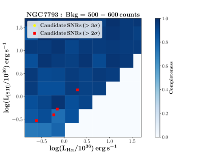
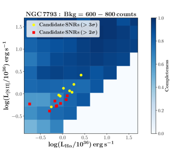
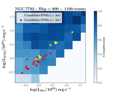
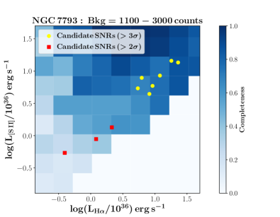
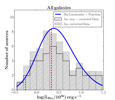
Figure 7 shows the binned differential incompleteness-corrected H${\rm\alpha}$ luminosity functions for the candidate SNRs in all galaxies (gray histogram). The incompleteness corrected number of sources for each luminosity bin is given by the sum $\rm\sum_{i}(1/I_{i})$ for all sources within each H$\alpha$ bin. For reference, the solid-line histogram shows the observed (uncorrected) binned H${\rm\alpha}$ luminosity distribution. We see, that as expected, in general, the effect of incompleteness is more significant for the lower luminosity sources. However, even in the bright end the completeness is never 100% because of the selection in the [S ii] emission lines and the high background in which we find the more luminous SNRs. The vertical dashed-lines show the H$\rm\alpha$ luminosity limit for the different galaxies (red, green, orange, and magnenta for NGC 55, NGC 7793, NGC 1313, and NGC 45 respectively). The fact that in the H$\rm\alpha$ LF we include also the galaxies NGC 45 and NGC 1313 for which the lowest luminosity limit is higher than NGC 55 and NGC 7793, does not affect significantly the shape of the H$\rm\alpha$ LF, since these galaxies have a very small number of SNRs. Furthermore the LF does not show any features at the location of the luminosity limits for each sample. In fact jointly fitting the four individual LFs (leaving free their normalizations) gives very similar results for their shape parameters.

We fit the $\rm LF_{H{\alpha}}$ by performing a maximum likelihood fit on the un-binned data. We fit a model described by a skewed Gaussian function (in the log(L)) in order to account for the asymmetric shape of the LFs (Figure 7). The skewed-Gaussian distribution is given by the function:

$$\rm{f(logL)=\frac{A}{\sigma\sqrt{(2\pi)}}e^{\frac{-(logL-\mu)^{2}}{2\sigma^{2}}}\{1+erf[\frac{\alpha(logL-\mu)}{\sigma\sqrt{2}}]\}}$$ (1)

where $\rm\mu$ is the mean of the distribution, $\rm\sigma$ the standard deviation, and $\rm\alpha$ the skewness parameter which describes the asymmetry of the LF and potential selection effects. The incompleteness is included as a weight term in the likelihood function.

The amplitude (A), of the function reflects the total number of SNRs ($\rm N_{Total}$). The number of incompleteness corrected objects down to our faintest limit is calculated by $\rm K=\sum_{i=0}^{N}(1/I_{i})$, where N is the total number of observed sources in each galaxy. Since the function used to model the luminosity function is normalized, the total number of incompleteness corrected objects (even beyond the faintest limit) and hence the amplitude factor A in eq. 1 is given by $\rm A=N_{Total}=K/\int_{log{(L_{min})}}^{log{(L_{max})}}f(log(L))d(log(L))$, where $\rm L_{min}$ and $\rm L_{max}$ are the minimum and maximum luminosity (in this case H$\alpha$ luminosity) of our sample.

For the determination of the best fit model parameters we used a Markov Chain Monte Carlo method implemented in the python package pymc. We assume flat priors for all the parameters of interest ($\rm\mu,\,\sigma,\,and\,\alpha$) and we perform 40000 iterations (excluding 500 burn-in iterations). The best-fit parameters and their uncertainties (at the 68% percentile) as derived by the posterior distribution of the model parameters are given in Table 5. The best-fit model to the un-binned data is shown as the solid line in Figure 7.

In Table 5 we also give the number of the detected SNRs (N) and the total number of SNRs (A; i.e. after accounting for incompleteness) of the overall sample of the 4 galaxies, and we calculate the detection fraction, which is the ratio of the number of the detected sources over the total number of SNRs ($\rm N/A$). As we see, the detected SNRs can be $\sim$ 30% less than the total number of SNRs in a galaxy. We can also estimate the total, incompleteness corrected, number of SNRs for each galaxy individually, down to the lowest H$\rm\alpha$ luminosity limit of the global H$\rm\alpha$ LF. To do that, we calculate the $\rm{N_{i}}\times\frac{\int_{L_{min,i}}^{\infty}LF(L_{H\rm\alpha})dL_{H\rm\alpha}}{\int_{L_{min}}^{\infty}LF(L_{H\rm\alpha})dL_{H\rm\alpha}}$, where ${L_{min,i}}$ is the lowest H$\rm\alpha$ luminosity of each galaxy $i$, $N_{i}$ is the incompleteness corrected number of sources of each galaxy, and ${L_{min}}$ is the lowest H$\rm\alpha$ luminosity of our total sample. This analysis gives 14.8, 5.8, 13.5, and 32.6 candidate SNRs for NGC 45, NGC 55, NGC 1313, and NGC 7793 respectively.

If we take into account also the possible candidate SNRs ([S ii]/H$\rm\alpha$ ratio 2$\rm\sigma$ above the 0.4 threshold) we find for the H$\rm\alpha$ LF $\rm\mu=-0.37^{+0.79}_{-0.01},\,\sigma=0.61^{+0.17}_{-0.03}$ and $\rm\alpha=1.09^{+0.20}_{-0.50}$.

Table 5: H$\rm{\alpha}$ Luminosity Function parameters for candidate SNRs (>3$\rm\sigma$)

N	$\rm{\mu}\,(log(L^{*}))$	$\rm{\sigma}\,(log(L^{*}))$	$\rm{\alpha}$	$\rm N_{max}$	$\rm A$	Detection Fraction
42	$\rm 0.07^{+0.63}_{-0.05}$	$\rm 0.58^{+0.11}_{-0.09}$	$\rm 1.70(>0.48)$	$\rm 8.62\pm 1.32$	59.83 $\pm$ 9.17	0.70 $\pm$ 0.10

• Col (1): the number of candidate SNRs (> 3$\rm\sigma$) of all galaxies; col (2) and col (3): the mean and sigma of the H$\rm\alpha$ luminosity function respectively; col (4): the skewness parameter of the H$\rm\alpha$ luminosity function; col (5): the model-based number of sources at the bin corresponding to the peak of the distribution; col (6): the total number of SNRs; col (7): the ratio of the number of the detected sources over the total number of SNRs ($\rm N/A$).
  ^∗Luminosity in units of $\rm 10^{36}$ erg s^-1
  

Figure 7: The incompleteness-corrected H$\rm\alpha$ luminosity function of the candidate SNRs (with ([S ii]/H$\rm\alpha$ - 0.4) > 3$\rm\sigma$; gray histogram), plotted along with the observed luminosity function without any incompleteness correction (black-line histogram). The blue curve shows the best-fit $\rm LF_{H\alpha}$ fitted to the incompleteness-corrected data. The vertical dashed-lines present the faintest H$\rm\alpha$ luminosity limits of the candidate SNRs in the galaxies NGC 55 (red), NGC 7793 (green), NGC 1313 (orange), and NGC 45 (magenta).

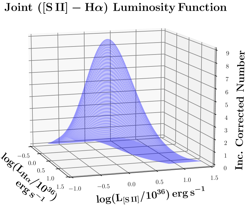
5.2.2 The joint [S II] - H$\rm{\alpha}$ luminosity function

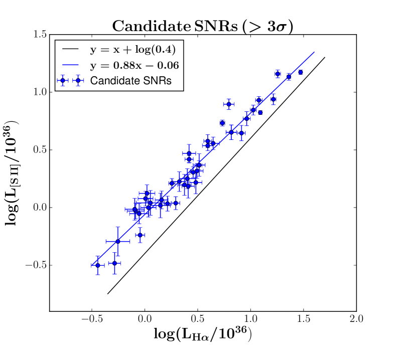
Since we have measurements of both the H$\rm\alpha$ and [S ii] luminosities of the SNRs in our sample, we can also calculate their joint luminosity function (LF) which yields information on the luminosity and excitation of the SNR populations. The location of the sources on the H$\rm\alpha$ - [S ii] luminosity plane is shown in Figure 11.

To quantify the shape of the [S ii]-H$\rm\alpha$ joint distribution for the candidate SNRs (and not the possible candidate SNRs), we adopt the following approach. We first calculate the relation between the $\rm log(L_{[S\,II]})$ and $\rm log(L_{H\alpha})$ luminosity for the detected sources. The best-fit relation is log([S ii]) = 0.88log(H$\rm\alpha$) - 0.06. This is the "spine" of the distribution of the candidate SNRs on the [S ii]-H$\rm\alpha$ plane, shown by the blue line in Figure 11.

Then, we project all the points on the best-fit line (i.e. for each H$\rm\alpha$ we calculate the log([S ii]) - y = log([S ii]) - (0.88log(H$\rm\alpha$) - 0.06)). We then fit a skewed Gaussian to the distribution of these points along the best-fit line, applying the incompleteness correction for each source (considering each source $\rm i$ as $\rm 1/Ii$; $\S$ 5.2.1). As for the H$\rm\alpha$ LF, we use a Markov Chain Monte Carlo method, assuming flat priors for all the parameters of interest ($\rm\mu,\,\sigma,\,and\,\alpha$) and performing 40000 iterations (excluding 500 burn-in iterations). The best-fit parameters of the 2D LF, are presented in Table 6. If we take into account also the possible candidate SNRs ([S ii]/H$\rm\alpha$ ratio 2$\rm\sigma$ above the 0.4 threshold) the the parameters $\rm\mu,\,\sigma$ and $\rm\alpha$ parameters of the 2D [S ii] - H$\rm\alpha$ LF are $-0.34^{+0.66}_{-0.04}$, $0.53^{+0.14}_{-0.03}$ and $0.57^{+0.67}_{-0.07}$ respectively.

Aiming to obtain a full picture of the 2D H$\rm\alpha$ - [S ii], we also need to measure the scatter of the candidate SNRs around the "spine" of the [S ii] - H$\rm\alpha$ distribution (the best-fit line derived above). In order to do so, we calculate the distance of each source from the best-fit [S ii] - H$\rm\alpha$ line, on the [S ii] axis. The distribution of these distances is described by a truncated Gaussian the fit parameters of which have been calculated using the same approach as above. The $\rm\mu$ and $\rm\sigma$ values of the truncated Gaussian are $0.024^{+0.025}_{-0.024}$ and $0.14^{+0.018}_{-0.029}$ respectively. The sigma is considered as the width of the 2D LF. The joint [S ii]-H$\rm\alpha$ LF is presented in Figure 11.

The total number of SNRs may be affected by the number of false positives: i.e. sources which satisfy the [S ii]/H$\rm\alpha$ > 0.4 criterion even at the 3$\rm\sigma$ level, while in reality they have lower [S ii]/H$\rm\alpha$ ratios. Such sources could be H ii regions, with [N ii]/H$\rm\alpha$ ratio different than the one that we have adopted for our analysis. However, based on the analysis presented in §4.1 we calculate that the fraction of sources with intrinsic [S ii]/H$\rm\alpha$ ratios between 0.2-0.3 and 0.3-0.4, that are found to satisfy our [S ii]/H$\rm\alpha$ > 0.4 criterion at the 3$\rm\sigma$ level, is only 0.3% - 1.0% for the different galaxies in our sample and for the different backgrounds in each galaxy. Therefore, we consider the contamination by lower excitation sources negligible.

Table 6: [S ii] - H$\rm{\alpha}$ Luminosity Function parameters for candidate SNRs (>3$\rm\sigma$)

$\rm Axis$	$\rm N$	$\rm{\mu}\,(log(L^{*}))$	$\rm{\sigma}\,(log(L^{*}))$	$\rm\alpha$	$\rm{N_{max}}$	$\rm A$	Detection fraction
$\rm L=0.88log(L_{H\alpha})-0.06$	42	$-0.03^{+0.56}_{-0.03}$	$0.48^{+0.13}_{-0.05}$	1.73(>1.69)	7.62 $\pm$ 1.17	59.38 $\pm$ 9.10	0.71 $\pm$ 0.01
$\rm log(L_{[S\,II]}/10^{36})$	-	$0.024^{+0.025}_{-0.024}$	$0.14^{+0.02}_{-0.03}$	-	-	-	-

• Col (1): the number of candidate SNRs (>3$\rm\sigma$) of all galaxies; col (2) and col (3): the mean and sigma values of the joint [S ii] - H$\rm\alpha$ luminosity function respectively (for the skewed Gaussian along the line $\rm y=0.88x-0.06$ which shows the shape of the LF; first row, and for the truncated Gaussian on the [S ii] axes, i.e the distance of the [S ii] from the line $\rm y=0.88x-0.06$, which shows the width of the LF; second row); col (4): the skewness parameter of the joint [S ii] - H$\rm\alpha$ luminosity function; col (5): the model-number of the sources at the bin that corresponds to the peak of the distribution; col (6): the total number of candidate SNRs (even beyond the lower limit); col (7): the ratio of the number of the detected sources over the total number of candidate SNRs ($\rm N/A$).
  ^∗ $\rm L=0.88log(L_{H\alpha})-0.06$ (first row), and $\rm L=L_{[S\,II]}$ (second row), in units of $\rm 10^{36}$ erg s^-1

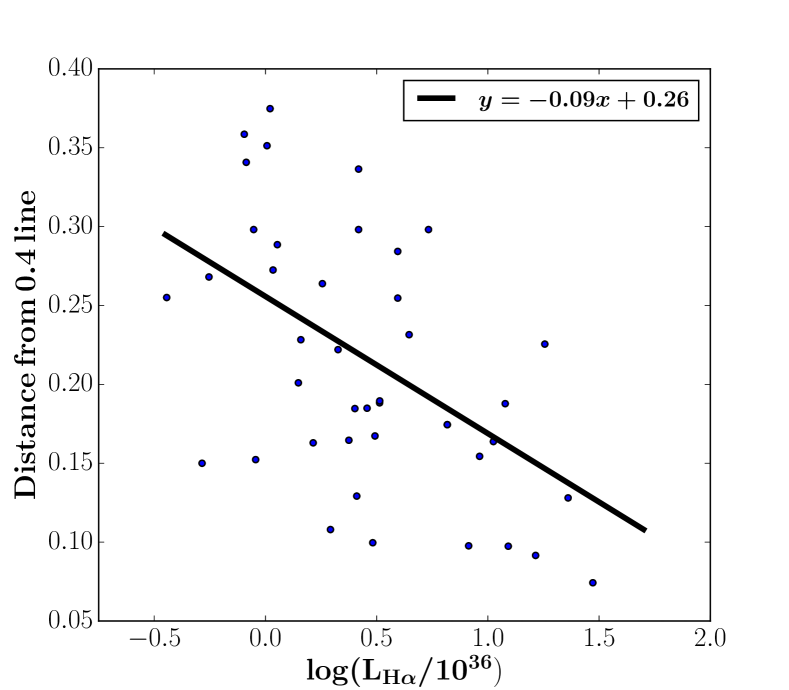
5.3 Excitation Function

An alternative way to view the 2D luminosity function, is in terms of the excitation of the SNRs, which is described by their [S ii]/ H$\rm\alpha$ ratio. The ratio of the forbidden and Balmer lines is an indicator of the degree of excitation of the emitting material. Therefore the range of this ratio can be used as a proxy for the physical condition in the SNR population (particularly in combination with shock excitation models). For this reason, we calculate the number density of SNRs, as function of their distance from the limiting [S ii]/H$\rm\alpha$ = 0.4 line, which is the threshold for SNR classification.

In Figure 11, this distance corresponds to different [S ii]/H$\rm\alpha$ ratios (i.e. different excitation). As we can see, there is a trend for SNRs with higher H$\rm\alpha$ luminosity, to present increasingly lower excitation. To quantify this trend, we fit a linear relation to the orthogonal distances from the 0.4 line, as function of the H$\rm\alpha$ luminosity: D $=$ $\rm\alpha$log(H$\rm\alpha$) $+$ $\rm\beta$ (Figure 11). We find $\rm\alpha=-0.09$ and $\rm\beta=0.26$, indicating a sub-linear relation, i.e. more luminous objects tend to have lower excitation.

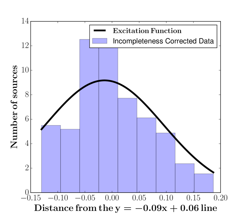
We introduce the excitation function as the vertical distribution of the candidate SNRs with respect to $\rm D=-0.09log(H\alpha)+0.26$ (Figure 11). Then, we calculate the distance of each source from this line, in order to quantify the spread around the excitation function. The difference between the excitation function and the 2D [S ii] - H$\rm\alpha$ LF, is that in the latter, the y-dimension corresponds to the [S ii] luminosity. While one can derive the excitation function from the 2D [S ii] - H$\rm\alpha$ LF, for simplicity and more direct assessment of the excitation of SNRs, we also introduce the excitation function. The distribution of these distances are presented in Figure 11 (blue histogram).

This distribution is described by a truncated Gaussian, the best parameters of which are: $\rm\mu=-0.014^{+0.011}_{-0.051}\,and\,\sigma=0.11^{+0.04}_{-0.21}$. The fitted truncated Gaussian has been calculated for the incompleteness-corrected candidate SNRs and it is presented in Figure 11 (black line). If we take into account also the possible candidate SNRs ([S ii]/H$\rm\alpha$ ratio 2$\rm\sigma$ above the 0.4 threshold) the parameters $\rm\mu$, and $\rm\sigma$ of the excitation function are $-0.004^{+0.009}_{-0.014}$, and $0.10^{+0.01}_{-0.19}$ respectively. In this case the sub-linearity is characterized by a slope -0.10.

Figure 8: A scatter plot of the [S ii] and H$\rm\alpha$ luminosity of the candidate SNRs. The black line shows the [S ii]/H$\rm\alpha$ = 0.4 threshold. The blue line shows the best-fit log($\rm L_{[S\,II]}$) - log($\rm L_{[H\alpha}$) relation for the sample of candidate SNRs.

Figure 9: The joint [S ii] - H$\rm\alpha$ luminosity function along the best-fit line: $\rm log(L_{[S\,II]}/10^{36})=0.88log(L_{[H\alpha}/10^{36})-0.06$. The parameters of the joint LF are presented in Table 6. In order to obtain the 3D interpretation, we multiply the skewed Gaussian that describes the shape of the joint LF along the best-fit line, with the truncated Gaussian that describes the width of the joint LF on the [S ii] dimension.

Figure 10: The points show the distance of each source from the [S ii]/H$\rm\alpha$ = 0.4 line. The black line is the best fit line that describes the distance of the candidate SNRs from the [S ii]/H$\rm\alpha$ = 0.4 line as function of their H$\rm\alpha$ luminosity.

Figure 11: The histogram is the incompleteness-corrected source distance from the best-fit line of Figure 11 distribution ($\S$ 5.3), and the black line is the fitted excitation function, described by a truncated Gaussian with $\rm\mu(log(L_{[S\,II]}/10^{36}))=0.024$ and $\rm\sigma(log(L_{[S\,II]}/10^{36}))=0.14$.

6 Discussion

6.1 Comparison with other surveys

In our survey we have detected in total 42 candidate SNRs (30 of which are new identifications) and 54 new possible candidate SNRs. This is a significant contribution to the number of known optical extragalactic SNRs. In addition, we find 21 sources with [S ii]/H$\rm\alpha$ > 0.4 at both 3$\rm\sigma$ and 2$\rm\sigma$ levels, which are associated with larger structures. The size of these structures ranges from $\sim$ 40 to $\sim$ 320 pc. Larger structures with size between $\sim$40 and $\sim$100 pc are most probably more evolved SNRs (Franchetti et al. 2012), while those with diameter larger than 100 pc are likely super-bubbles or groups of SNRs. For the largest such SNRs, with diameter of $\sim$100  pc, and assuming that the density of the surrounding ISM is 10 $\rm cm^{-3}$ and the explosion energy was $\rm 10^{51}\,erg$, according to Sedov-Taylor solution (Draine 2011), its age is $\sim$100000 years, i.e. an old SNR.

In this study we present for the first time optical SNR candidates in NGC 45, NGC 55, and NGC 1313. NGC 7793 has been studied before by Blair & Long (1997) who presented 27 SNRs. Almost all these SNRs have been also identified in our deeper survey which yields 24 candidate SNRs (13 of which coincide with those of Blair & Long 1997) and 31 possible candidate SNRs. Five of the SNRs that are reported in the work of Blair & Long (1997) (s2, s3, s7, s18, s2, s26ext) coincide with 5 (out of 8) larger structures that we detected in this galaxy. Some SNRs in the study of Blair & Long 1997 have [S ii]/H$\rm{\alpha}$ ratio less than 2$\rm{\sigma}$ above the 0.4 limit in our study so they are not discussed in this paper (s9, s17, s21, s22). We do not identify as SNRs sources s19, s23, s15 in the catalogue of Blair & Long (1997). Sources s4, s19 and s15 have [S ii]/H$\rm{\alpha}$ ratio 0.36, and 0.17 respectively, i.e. below our 0.4 limit. Source s23 instead, is resolved into multiple sources in our images none of which gives high [S ii]/H$\rm{\alpha}$ ratio. Source s27 in our images appears as a faint ring. Since our study focuses on more point-like sources, we do not detect shell-like sources (unless they present knots that satisfy our selection criteria as discussed in $\S$ 5), which however, are not included in our luminosity and excitation functions.

Large samples of extragalactic SNRs have been presented in many surveys. In M31 (Lee & Lee 2014a) and M33 (Lee & Lee 2014b) have been detected 156 and 199 photometric SNRs respectively. Matonick & Fesen (1997) identified 93 SNRs in M101 and 41 SNRs in M81. Surveys led by Blair et al. (2014), Dopita et al. (2010) and Blair & Long (2004) have given 296 SNRs in M83. Leonidaki, Boumis, & Zezas (2013), in a survey of 6 galaxies presented 149 photometric SNRs in NGC 2403, 92 in NGC 4214, 70 in NGC 4449, 47 in NGC 4395, 36 in NGC 5204 and 24 in NGC 3077. The most recent work on NGC 6946, gave 147 photometric SNRs (Long et al. 2019). The number of detected SNRs depends on various characteristics of a galaxy (e.g. SFR; ISM density distribution etc.) but also on the sensitivity of the observations and the distance of the galaxy. However, a fair comparison between different studies requires the application of the incompleteness corrections we described in this work.

6.2 Multi - wavelength comparison

By construction of our sample, the four galaxies we consider in this study have been observed in the X-rays with the Chandra X-ray Observatory. These observations reach limiting luminosities of $3\times 10^{37}\,\rm erg\,s^{-1}$, $6.8\times 10^{36}\,\rm erg\,s^{-1}$ , $7.4\times 10^{36}\,\rm erg\,s^{-1}$, and $3.3\times 10^{36}\,\rm erg\,s^{-1}$ for NGC 45, NGC 55, NGC 1313, and NGC 7793 respectively (Wang et al. 2016). As we would expect the fainter limit is higher for the more distant galaxies. Next we discuss the multi-wavelength (X-ray, radio, optical) populations of SNRs in our sample galaxies, focusing on published samples of SNRs in the X-ray and radio bands. A more detailed study of the X-ray emission of SNRs based on a reanalysis of the existing data will be published in a forthcoming paper. In Table 7 we present the candidate SNRs of the galaxies of our study, along with their counterparts from other studies. Following, we discuss in more detail these comparisons. In NGC 45, we find that none of the optically detected SNRs has any counterpart in radio or X-ray wavelengths (Pannuti et al. 2015). In NGC 55, only source 1 from the possible candidate SNRs has also emission in X-rays (source 131 in Binder et al. 2015, or source 85 in Stobbart, Roberts, & Warwick 2006). The fact that in the optical band we detect only 1 source out of the 18 X-ray SNRs, is probably an age effect (although we cannot exclude the possibility of ISM differences, especially given the fact that NGC 55 has different morphology from the other 3 galaxies in our sample; c.f. Leonidaki, Zezas, & Boumis, 2010). The blast waves of very young SNRs heat the material behind the shock front to very high temperatures ($\rm\sim 10^{7}\,K$) producing thermal X-rays (e.g. Ramakrishnan & Dwarkadas 2020; Maggi et al. 2016; Leonidaki, Zezas, & Boumis 2010). Most SNRs that produce X-ray emission are in the phase of free expansion or in the early adiabatic phase (e.g. Vink 2012) where we do not expect strong optical emission. Moreover, the SNR J001514-391246 in O’Brien et al. (2013), which emits in radio and X-rays, presents a shell-like structure ($\rm\sim 44\,pc$) in our H$\rm\alpha$ image. Such SNRs would not be detected efficiently in our survey, which focuses on point-like sources. However, we find that this specific SNR does not show strong [S ii] emission indicating that it could be embedded in H ii region.

In NGC 1313, we do not detect any of the young X-ray emitting SNRs reported in Colbert et al. (1995). We see strong H$\rm\alpha$ emission at the position of SN 1978K which emits in the X-rays (Smith et al. 2007; Colbert et al. 1995; Schlegel, Petre, & Colbert 1996; Petre et al. 1994) and in radio (Achterberg & Ball 1994), but its low [S ii] emission indicates that the shock may have not excited enough material to make it visible as an optical SNR.

In NGC 7793 the candidate SNR 22 coincides with a radio SNR of the work of Pannuti et al. (2002). Two of the 3 optically selected radio SNRs of Galvin et al. (2014) (29, 31) coincide with our candidate SNRs 22 and 19 respectively. The third optically selected radio SNR of the same work (58) has been also identified in our study but with a significance below 2$\rm\sigma$ so it is not considered here. The larger structure 6 has been detected in the radio (Pannuti et al. 2002) and in X-rays (Pannuti et al. 2011). However, we do not consider this structure as an SNR but rather as a super-bubble because of its large size ($\sim$ 320 pc). This is confirmed by the work of Dopita et al. (2012) who suggest that it is a super-bubble created by a microquasar.

Table 7: Comparison with other studies

ID	RA	Dec	Other surveys
	(J2000)	(J2000)
	hh:mm:ss	dd:mm:ss
NGC 55
1	00:15:43.2	-39:16:03.0	131∗ (Binder et al. 2015)
NGC 7793
1	23:57:45.0	-32:37:40.2	S8 (Blair & Long 1997)
3	23:58:06.5	-32:35:37.0	S28 (Blair & Long 1997)
4	23:57:38.7	-32:34:38.5	S1 (Blair & Long 1997)
6	23:57:52.6	-32:33:54.4	S14 (Blair & Long 1997)
9	23:57:41.1	-32:37:02.1	S5 (Blair & Long 1997)
13	23:57:54.5	-32:35:12.2	S16 (Blair & Long 1997)
18	23:57:56.1	-32:37:18.5	S20 (Blair & Long 1997)
19	23:57:48.3	-32:36:55.2	S12 (Blair & Long 1997)
			31∗∗ (Galvin et al. 2014)
20	23:57:51.2	-32:36:31.7	S13 (Blair & Long 1997)
21	23:57:59.2	-32:36:06.0	S24 (Blair & Long 1997)
22	23:57:47.3	-32:35:23.9	S11 (Blair & Long 1997)
			29∗∗ (Galvin et al. 2014)
			S11 (Pannuti et al. 2002)
23	23:57:45.8	-32:35:01.7	S10 (Blair & Long 1997)

The sources from the work of Blair & Long (1997) are optical SNRs.
^∗ X-ray SNRs
^∗∗ Radio SNRs

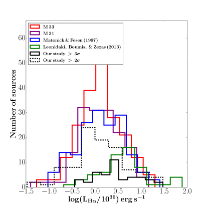
6.3 The H$\rm\alpha$ Luminosity Function of SNRs

In Figure 12, we compare the ${\rm{H\alpha}}$ luminosity distribution of our candidate SNRs (black solid line) and the possible candidate SNRs (black dashed line), with the spectroscopic SNR population in the study of Leonidaki, Boumis, & Zezas (2013; NGC 2403, NGC 4212, NGC 3077, NGC 4395, NGC 4449, NGC 5204), and photometric SNRs in the studies of Matonick & Fesen (1997; NGC 5585, NGC 6946, M81, M101), Lee & Lee (2014a; M31) and Lee & Lee (2014b; M33).

Our candidate SNRs, which is the more secure sample of the two, seem to more closely follow the distribution of the spectroscopic SNRs of Leonidaki, Boumis, & Zezas (2013) while the distribution of the possible candidate SNRs agree with the distribution of the photometric SNRs of the other studies. This is expected since our sample of candidate SNRs consists of brighter objects (since they have higher signal to noise ratio in the [S ii]/H$\rm\alpha$ ratio), and by necessity, spectroscopic surveys also target brighter objects.

In general, the distribution of the ${\rm{H\alpha}}$ luminosity of our candidate SNRs appear to be flatter compared to the other studies. This is the result of the strict selection criterion, [S ii]/H$\rm\alpha$ ratio to be 3$\rm\sigma$ above the 0.4 threshold, which is not used in the other surveys. Indeed, we see that the less accurate sample ([S ii]/H$\rm\alpha$ ratio 2$\rm\sigma$ above the 0.4 threshold; black dashed line), agrees more with the other studies.

What distinguishes our work from the previous efforts is that: (a) we account for the effects of incompleteness, which allows us to study more accurately the faint end of their distribution and (b) we provide a quantitative description of the LFs, which can be used for comparison between different samples and theoretical models for the population of SNRs in different environments.

Figure 12: Comparison of the ${\rm{H\alpha}}$ luminosity distribution of our candidate SNRs (black solid line), our possible candidate SNRs (black dashed line) and the studies of spectroscopic SNRs from Leonidaki, Boumis, & Zezas 2013 (green line), and photometric SNRs from Matonick & Fesen 1997 (blue line), M31 (Lee & Lee 2014a; purple line), and M33 (Lee & Lee 2014b; red line).

In Figure 7, we see the incompleteness-corrected luminosity distribution (gray histogram) and the best fit function (blue line) along with the initial, uncorrected data (black-line histogram). We see that apart from the different amplitudes, the mean value of a function that would describe the incompleteness uncorrected data would be shifted to the higher luminosities (since the incompleteness correction affects less the brighter sources) and the skewness would be different.

The skewness at the faint end of the LFs is due to incompleteness. In principle, the limited sensitivity of our survey and the selection of SNRs based on the [S ii]/H$\rm\alpha$ criterion may prevent us from observing the peak of the H$\rm\alpha$ LF of the overall SNR population, even for the nearest galaxies. In order to compare our results with the published photometric SNR samples, which do not impose any threshold on the significance of the [S ii]/H$\rm\alpha$ ratio, we use our less secure sample (> 2$\rm\sigma$), and we compare it with the luminosity distribution of SNRs in the Local Group M31 and M33 galaxies. We see (Figure 12) that both show a peak at $\rm L_{H\alpha}\sim 10^{36}\,erg\,s^{-1}$.

Taking into account the fact that the two surveys have similar flux sensitivity limits, while our objects lie at much larger distances, this strongly suggests that the peak in the H$\rm\alpha$ LF of SNRs, selected on the basis of the [S ii]/H$\rm\alpha$ criterion (at signal to noise ratio > 2 $\rm\sigma$ resulting in small contamination by H ii regions), is $\rm\sim 10^{36}\,erg\,s^{-1}$ as measured from our quantitative analysis. Focusing on results, e.g. by integrating the LF, we find that we are missing $\sim$ 30% of the SNR population down to our detection limit.

Vučetić et al. (2015) followed a similar approach for calculating the overall population of SNRs, by integrating a Gaussian distribution fitted to the bright-end of the H$\rm\alpha$ luminosity distribution of the photometric SNR populations in nearby galaxies. However this approach does not account for the effects of incompleteness which may impact even the higher luminosity objects.

In spiral galaxies $\sim 75\%$ of SN is core collapse (Vink 2020). We expect that the SNRs that we find in star-forming regions (such as those we consider here) are core collapse SNRs. Hence, since the majority of these SNRs depict the end-point of massive-stars life, they can be used as star formation rate (SFR) indicators. However, because of selection effects and incompleteness biases it cannot be used directly to derive the relation between SNRs and SFR, unless we correct for the incompleteness. The approach we have used in this work, can be used also to calculate a more reliable relation between the number of SNRs and SFR.

6.4 The bivariate LF and the degree of excitation

Observationally, because of the weakness of the [S ii]$\rm\lambda\lambda 6717,6731\AA$ lines, the [S ii]/H$\rm{\alpha}$ criterion generally poses a higher threshold in the SNR luminosity than the sensitivity of the H$\rm\alpha$ data. In fact, the [S ii]/H$\rm{\alpha}$ selection could be the main source of the skewness observed in the H$\rm\alpha$ LF (Figure 7). Similarly, this selection also results in the skewness observed in the ([S ii]-H$\rm{\alpha}$) bivariate LF along the main axis ([S ii]/H$\rm{\alpha}$; Figure 11). The truncation observed along the perpendicular (excitation) axis (Figure 11) is the result of the sharp [S ii]/H$\rm\alpha$ > 0.4 threshold.

Regarding the excitation function, as we see in Figure 11, there is a trend for sources with higher H$\rm\alpha$ luminosities to have increasingly lower [S ii]/H$\rm{\alpha}$ ratios (i.e. lower excitation) as is indicated by the sub-linear ($\alpha=-0.09$) slope of the $\rm log(L_{[S\,II]})-log(L_{H\alpha})$ relation in Figure 11. This effect would indicate that more luminous objects have lower excitation, which is counter-intuitive since these are expected to be the younger SNRs, and hence the ones with faster shocks and higher excitation. On the other hand, it is more likely that this is an observational effect: luminous SNRs are more likely to be in regions with high ISM density and possibly embedded in H ii regions (e.g. Arbutina & Urošević 2005). Indeed, this is a trend that we see in Figure 6, where more luminous SNRs are located in regions with higher backgrounds. We note that this cannot be a selection bias, since brighter objects should be detectable in lower backgrounds as well. This is also one of the reasons (along with the incompleteness due to the [S ii] and the strict selection criterion for the [S ii]/H$\rm\alpha$ at 3$\rm\sigma$), that the completeness is not 100% even for the brighter sources, while is low at the faint end of the H$\rm\alpha$ LF (Figure 7), where the sources are found in lower background regions. The contamination by the underlying emission from the H ii regions would result in higher H$\rm\alpha$ luminosities but disproportionally lower [S ii] luminosities due to the lower [S ii]/H$\rm{\alpha}$ ratios of the H ii regions.

At first glance this may sound at odds with our expectations that more luminous SNRs are expected to energise more efficiently their surrounding medium. However, this could also be a result of the [S ii]/H$\rm{\alpha}$ selection criterion which biases against lower excitation objects. Only including a more complete population of objects (e.g. based also on the [O i]/H$\rm\alpha$ criterion e.g. Kopsacheili, Zezas, & Leonidaki 2020; Fesen et al. 1985) we may draw more robust conclusions on the excitation function and the degree of energization of the local ISM.

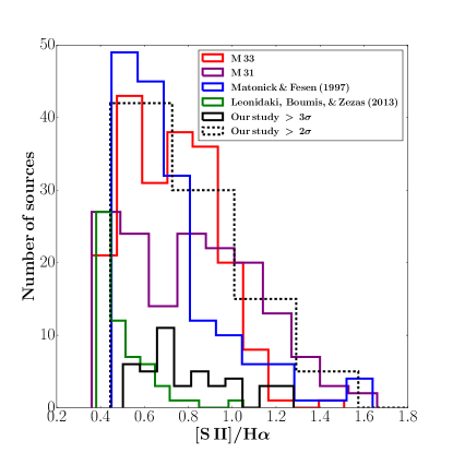
In Figure 13, we compare the distribution of the [S ii]/H$\rm{\alpha}$ ratios of the candidate SNRs (black solid line) and the possible candidate SNRs (black dashed line) detected in our survey and those reported in the surveys of Leonidaki, Boumis, & Zezas (2013), Matonick & Fesen (1997), and Lee & Lee (2014a, b), aiming to examine the SNR excitation between different galaxies. The range of the [S ii]/H$\rm{\alpha}$ values of our possible candidate SNRs is more similar to the values of the SNRs of the other surveys, although the distributions are not the same, while the [S ii]/H$\rm{\alpha}$ ratios of our candidate SNRs is quite different.

The difference, between our sample and the other studies in the faint end has to do with the different adopted [S ii]/H$\rm{\alpha}$ ratio to identify SNRs (for our possible candidate SNRs), and with the fact that our selection criterion in the [S ii]/H$\rm{\alpha}$ ratio (3$\rm\sigma$ above 0.4) is satisfied only for sources with high [S ii]/H$\rm{\alpha}$ ratios (for our candidate SNRs). The general difference in the [S ii]/H$\rm{\alpha}$ ratio distributions, between our possible candidate SNRs and the other surveys (that do not impose any threshold at the significance level of the [S ii]/H$\rm{\alpha}$ ratio), may have to do with the different ISM conditions of the galaxies, but also with the different sensitivity between the studies. This emphasises the need for incompleteness corrections also in the [S ii]/H$\rm\alpha$ ratio distributions.

Figure 13: Histograms of the distribution of the [S ii]/H$\rm{\alpha}$ ratios for the SNRs in our sample (black solid line for the candidate SNRs; black dashed line for the total sample, i.e. the candidate and the possible candidate SNRs), Leonidaki, Boumis, & Zezas (2013; green line), Matonick & Fesen (1997; blue line), M31 (Lee & Lee 2014a; purple line), and M33 (Lee & Lee 2014b; red line).

6.5 The effect of [S  II]/H$\rm{\alpha}$ > 0.4 criterion

Correcting our data for incompleteness, gives us the possibility to recover a number of SNRs that we did not detect (due to their faintness, their galactic environment etc.) down to our faintest detection limit. However, there is a number of SNRs that we do not detect due to selection criteria: for example, the [S ii]/H$\rm{\alpha}$ > 0.4 criterion which is biased against low velocity SNRs.

If the SNRs with [S ii]/H$\rm{\alpha}$ < 0.4 follow the extension of the distribution that we derived from those with [S ii]/H$\rm{\alpha}$ > 0.4, we can estimate the fraction of SNRs that we miss because of the [S ii]/H$\rm{\alpha}$ selection criterion. Then, the missing population is given by the extrapolation of the best-fit truncated Gaussian (Figure 11) to lower [S ii]/H$\rm{\alpha}$ ratios, after removing the truncation term. Applying this method on the best fit truncated Gaussian to the excitation function of SNRs, we find that almost 47% of the overall SNR population is not accounted for, under the assumption that the distribution of [S ii]/H$\rm{\alpha}$ > 0.4 extends to lower [S ii]/H$\rm{\alpha}$ flux ratios.

However, the [S ii]/H$\rm{\alpha}$ > 0.4 criterion is an empirical diagnostic that comes from studies of SNRs in the SMC and the LMC (Mathewson & Clarke 1973). As discussed in Kopsacheili, Zezas, & Leonidaki (2020), such a criterion may miss legitimate SNRs with relatively low shock velocities which result in lower [S ii]/H$\rm{\alpha}$ ratios (Allen et al. 2008). Such low velocities are characteristic of older SNRs (e.g. Draine 2011) or they may reflect their local ISM conditions (e.g. SNRs expanding in dense environments lose quickly their momentum and they slow down faster; e.g. Jiménez, Tenorio-Tagle, & Silich 2019; Cioffi, McKee, & Bertschinger 1988). Therefore, in order to have a more reliable picture of the overall SNR population one would need to combine fast-shock sensitive indicator (such as [S ii]/H$\rm{\alpha}$) with a slow-shock indicator (such as the [O i]/H$\rm{\alpha}$; Kopsacheili, Zezas, & Leonidaki 2020; Fesen et al. 1985).

7 Conclusions

In this work, we present the systematic study of optical SNR populations in 4 nearby spiral galaxies: NGC 45, NGC 55, NGC 1313, and NGC 7793. We identify 42 candidate and 54 possible candidate SNRs (84 of which are new identifications) detected at the 3$\rm\sigma$ level in deep H$\alpha$ images and selected on the basis of their [S ii]/H$\alpha$ flux ratios (higher than 0.4 at the 3$\rm\sigma$ and 2$\rm\sigma$ level respectively) following a fully automated procedure.

Based on this sample, we calculate the H$\alpha$ luminosity function and the joint H$\alpha$-[S ii] luminosity function after accounting for incompleteness effects. The latter presents a new way to encode the luminosity and excitation of the SNR populations. We model the luminosity function with a skewed Gaussian distribution. We find that the H$\alpha$ luminosity at the peak (mean) of the distribution of the overall sample (candidate and possible candidate SNRs) is $\rm\sim 10^{36}\,erg\,s^{-1}$. This is consistent with the peak of the H$\alpha$ luminosity distribution in SNRs detected in the M31 and M33 spiral galaxies for the same quality of data (also less accurate sample).

This is a pilot study to demonstrate the automated method for the identification of SNRs, the two new metrics of their SNR populations we introduced, and the application of incompleteness effects. This method will be applied to a larger and more diverse sample of galaxies in order to compare the characteristics of SNR populations in diverse environments.

We also find that SNRs with higher H$\alpha$ luminosity, tend to have lower excitation (i.e. lower [S ii]/H$\alpha$ ratio), although this could be an environmental effect. This can be seen directly by our data, where brighter sources are located in regions with higher backgrounds. The excitation function of the overall SNR population is modeled by a truncated Gaussian with the truncation accounting for the [S ii]/H$\alpha$ selection effect. We find that the width of the Gaussian is 0.11 in terms of distance (from the line $\rm y=-0.09x+0.26$).

DATA AVAILABILITY

The data underlying this article are available in the article and in its online supplementary material. The raw data are available from the NOAO data archives.

Appendix A Possible candidate SNRs (<$\rm 3\sigma$)

In LABEL:table:SNRs_total_2s we present the possible candidate SNRs, i.e. SNRs with 2$\rm\sigma$ < [S ii]/H$\rm\alpha$ - 0.4 < 3$\rm\sigma$. The first column gives the ID of the source, the second and the third columns give the RA and Dec coordinates (in J2000), the fourth and fifth columns give the H$\rm{\alpha}$ and [S ii] fluxes with their uncertainties, and the sixth column gives the [S ii]/H$\rm{\alpha}$ ratio with its uncertainty.

Table 8: Possible candidate SNRs

ID	RA	Dec	$\rm{F_{H\alpha}}\pm\rm{\delta F_{H\alpha}}$	$\rm{F_{[\text{S\,{ii}}]}}\pm\rm{\delta F_{[\text{S\,{ii}}]}}$	$\frac{\rm{F_{[\text{S\,{ii}}]}}}{\rm{F_{H\alpha}}}\pm$ ($\rm{\delta}\frac{\rm{F_{[\text{S\,{ii}}]}}}{\rm{F_{H\alpha}}}$)
	(J2000)	(J2000)
	hh:mm:ss	dd:mm:ss	($\rm 10^{-16}\,erg\,s^{-1}\,cm^{-2}$)	($\rm 10^{-16}\,erg\,s^{-1}\,cm^{-2}$)
NGC 45 ($\rm 2\sigma$)
1	00:14:02.3	-23:10:27.5	6.3 $\pm$ 0.54	4.21 $\pm$ 0.64	0.67 $\pm$ 0.10
2	00:14:12.4	-23:10:27.1	16.5 $\pm$ 0.4	7.31 $\pm$ 0.30	0.44 $\pm$ 0.02
3	00:14:09.8	-23:09:52.4	2.79 $\pm$ 0.22	1.85 $\pm$ 0.24	0.66 $\pm$ 0.10
NGC 55 ($\rm 2\sigma$)
1	00:15:43.5	-39:16:41.3	7.48 $\pm$ 0.46	4.01 $\pm$ 0.4	0.54 $\pm$ 0.06
2	00:15:56.9	-39:15:45.3	1.84 $\pm$ 0.6	2.76 $\pm$ 0.45	1.5 $\pm$ 0.5
3	00:15:29.9	-39:14:15.0	2.8 $\pm$ 0.61	3.54 $\pm$ 0.7	1.3 $\pm$ 0.4
4	00:15:06.9	-39:12:24.4	3.45 $\pm$ 0.63	3.47 $\pm$ 0.64	1 $\pm$ 0.3
5	00:14:54.0	-39:11:51.5	11.4 $\pm$ 3.3	16.1 $\pm$ 2.3	1.4 $\pm$ 0.5
6	00:14:20.2	-39:10:09.0	1.3 $\pm$ 0.19	1.15 $\pm$ 0.22	0.88 $\pm$ 0.2
7	00:14:01.5	-39:10:21.0	3.15 $\pm$ 0.24	2.05 $\pm$ 0.29	0.65 $\pm$ 0.1
8	00:14:40.5	-39:08:53.6	3.13 $\pm$ 0.27	2.13 $\pm$ 0.34	0.68 $\pm$ 0.1
9	00:13:51.4	-39:08:46.7	0.702 $\pm$ 0.18	0.975 $\pm$ 0.2	1.4 $\pm$ 0.5
NGC 1313 ($\rm 2\sigma$)
1	03:18:01.6	-66:31:30.5	0.87 $\pm$ 0.24	1.77 $\pm$ 0.3	2 $\pm$ 0.7
2	03:18:09.3	-66:31:12.4	3.19 $\pm$ 0.46	2.42 $\pm$ 0.35	0.76 $\pm$ 0.2
3	03:18:17.5	-66:30:20.4	5.53 $\pm$ 0.98	5.58 $\pm$ 1.1	1 $\pm$ 0.3
4	03:17:38.0	-66:30:01.5	6.81 $\pm$ 0.33	3.66 $\pm$ 0.32	0.54 $\pm$ 0.05
5	03:17:47.5	-66:29:48.5	12.9 $\pm$ 0.4	6.56 $\pm$ 0.43	0.51 $\pm$ 0.04
6	03:18:39.5	-66:29:12.1	13.6 $\pm$ 1.2	8.47 $\pm$ 0.95	0.62 $\pm$ 0.09
7	03:18:33.1	-66:28:50.0	7.22 $\pm$ 0.81	5.35 $\pm$ 0.66	0.74 $\pm$ 0.1
8	03:18:36.3	-66:27:58.6	4.03 $\pm$ 0.43	2.97 $\pm$ 0.38	0.74 $\pm$ 0.1
NGC 7793 ($\rm 2\sigma$)
1	23:58:08.2	-32:36:41.2	4.3 $\pm$ 0.5	3.2 $\pm$ 0.34	0.74 $\pm$ 0.1
2	23:57:37.2	-32:36:32.1	3.6 $\pm$ 0.33	2.4 $\pm$ 0.36	0.67 $\pm$ 0.1
3	23:57:31.3	-32:34:50.9	1.5 $\pm$ 0.25	1.8 $\pm$ 0.32	1.2 $\pm$ 0.3
4	23:57:54.2	-32:37:17.3	4.1 $\pm$ 0.61	4.2 $\pm$ 0.83	1.0 $\pm$ 0.2
5	23:57:44.6	-32:37:03.4	7.4 $\pm$ 0.6	4.5 $\pm$ 0.62	0.61 $\pm$ 0.1
6	23:57:41.0	-32:36:54.9	5.5 $\pm$ 0.52	3.7 $\pm$ 0.54	0.66 $\pm$ 0.1
7	23:57:38.6	-32:34:49.1	1.1 $\pm$ 0.33	3.6 $\pm$ 0.45	3.3 $\pm$ 1.0
8	23:57:59.3	-32:34:37.3	4.4 $\pm$ 0.54	3.2 $\pm$ 0.59	0.74 $\pm$ 0.2
9	23:57:59.8	-32:34:26.4	7.8 $\pm$ 0.87	5.5 $\pm$ 0.59	0.71 $\pm$ 0.1
10	23:57:37.9	-32:33:53.2	3.1 $\pm$ 0.32	2.5 $\pm$ 0.48	0.79 $\pm$ 0.2
11	23:57:50.6	-32:33:13.8	4.5 $\pm$ 0.58	3.3 $\pm$ 0.52	0.73 $\pm$ 0.1
12	23:57:48.4	-32:36:42.8	3.9 $\pm$ 0.79	3.8 $\pm$ 0.76	0.96 $\pm$ 0.3
13	23:57:58.0	-32:36:37.7	6.1 $\pm$ 0.55	4.3 $\pm$ 0.66	0.7 $\pm$ 0.1
14	23:57:52.2	-32:36:15.5	11.0 $\pm$ 0.7	7.6 $\pm$ 1.1	0.69 $\pm$ 0.1
15	23:57:58.3	-32:36:08.3	9.0 $\pm$ 0.7	5.5 $\pm$ 0.73	0.61 $\pm$ 0.09
16	23:57:46.0	-32:36:06.1	5.1 $\pm$ 0.73	6.5 $\pm$ 1.2	1.3 $\pm$ 0.3
17	23:57:58.2	-32:36:02.1	2.4 $\pm$ 0.42	2.5 $\pm$ 0.57	1.0 $\pm$ 0.3
18	23:57:58.7	-32:35:56.4	2.2 $\pm$ 0.41	2.6 $\pm$ 0.44	1.2 $\pm$ 0.3
19	23:57:55.0	-32:35:51.3	2.1 $\pm$ 0.53	3.0 $\pm$ 0.61	1.5 $\pm$ 0.5
20	23:57:43.9	-32:35:33.1	2.3 $\pm$ 0.65	5.5 $\pm$ 0.71	2.4 $\pm$ 0.7
21	23:57:44.2	-32:35:19.4	5.5 $\pm$ 0.81	4.5 $\pm$ 0.75	0.81 $\pm$ 0.2
22	23:58:00.4	-32:35:14.3	4.9 $\pm$ 0.44	3.3 $\pm$ 0.45	0.67 $\pm$ 0.1
23	23:57:44.1	-32:34:55.4	5.3 $\pm$ 0.86	4.7 $\pm$ 0.99	0.89 $\pm$ 0.2
24	23:57:50.1	-32:34:44.4	4.0 $\pm$ 0.57	4.5 $\pm$ 0.75	1.1 $\pm$ 0.2
25	23:57:58.4	-32:34:41.3	5.1 $\pm$ 0.42	3.3 $\pm$ 0.5	0.64 $\pm$ 0.1
26	23:57:41.0	-32:34:35.7	2.6 $\pm$ 0.38	2.5 $\pm$ 0.5	0.95 $\pm$ 0.2
27	23:57:51.0	-32:34:28.9	9.2 $\pm$ 0.63	6.6 $\pm$ 0.91	0.72 $\pm$ 0.1
28	23:57:54.2	-32:34:16.4	1.5 $\pm$ 0.31	1.8 $\pm$ 0.39	1.2 $\pm$ 0.4
29	23:57:54.7	-32:35:35.5	2.4 $\pm$ 0.66	3.3 $\pm$ 0.61	1.4 $\pm$ 0.4
30	23:57:58.9	-32:35:32.2	7.4 $\pm$ 0.71	5.4 $\pm$ 0.94	0.73 $\pm$ 0.1
31	23:57:47.2	-32:34:28.3	13.0 $\pm$ 1.6	8.2 $\pm$ 0.97	0.62 $\pm$ 0.1

References

- Achterberg & Ball (1994) Achterberg A., Ball L., 1994, A& A, 285, 687
- Allen et al. (2008) Allen M. G., Groves B. A., Dopita M. A., Sutherland R. S., Kewley L. J., 2008, ApJS, 178, 20
- Arbutina & Urošević (2005) Arbutina B., Urošević D., 2005, MNRAS, 360, 76. doi:10.1111/j.1365-2966.2005.09033.x
- Annunziatella et al. (2013) Annunziatella M., Mercurio A., Brescia M., Cavuoti S., Longo G., 2013, PASP, 125, 68
- Bertin & Arnouts (1996) Bertin, E., & Arnouts, S. 1996, A&AS, 117, 393
- Bibby & Crowther (2010) Bibby J. L., Crowther P. A., 2010, MNRAS, 405, 2737. doi:10.1111/j.1365-2966.2010.16659.x
- Binder et al. (2015) Binder B., Williams B. F., Eracleous M., Plucinsky P. P., Gaetz T. J., Anderson S. F., Skillman E. D., et al., 2015, AJ, 150, 94
- Blair et al. (2014) Blair W. P., Chandar R., Dopita M. A., Ghavamian P., Hammer D., Kuntz K. D., Long K. S., et al., 2014, ApJ, 788, 55. doi:10.1088/0004-637X/788/1/55
- Blair et al. (2013) Blair, W. P., Winkler, P. F., & Long, K. S. 2013, ApJS, 207, 40
- Blair et al. (2012) Blair, W. P., Winkler, P. F., & Long, K. S. 2012, ApJS, 203, 8
- Blair & Long (2004) Blair W. P., Long K. S., 2004, ApJS, 155, 101. doi:10.1086/423958
- Blair & Long (1997) Blair, W. P., & Long, K. S. 1997, ApJS, 108, 261
- Boumis et al. (2009) Boumis P., Xilouris E. M., Alikakos J., Christopoulou P. E., Mavromatakis F., Katsiyannis A. C., Goudis C. D., 2009, A&A, 499, 789. doi:10.1051/0004-6361/200811474
- Boumis et al. (2004) Boumis P., Meaburn J., López J. A., Mavromatakis F., Redman M. P., Harman D. J., Goudis C. D., 2004, A&A, 424, 583
- Castellanos, Díaz, & Terlevich (2002) Castellanos M., Díaz A. I., Terlevich E., 2002, MNRAS, 329, 315. doi:10.1046/j.1365-8711.2002.04987.x
- Cioffi, McKee, & Bertschinger (1988) Cioffi D. F., McKee C. F., Bertschinger E., 1988, ApJ, 334, 252. doi:10.1086/166834
- Colbert et al. (1995) Colbert E. J. M., Petre R., Schlegel E. M., Ryder S. D., 1995, ApJ, 446, 177
- Condon & Yin (1990) Condon J. J., Yin Q. F., 1990, ApJ, 357, 97. doi:10.1086/168894
- Daltabuit et al. (1976) Daltabuit, E., Dodorico, S., & Sabbadin, F. 1976, A&A, 52, 93
- Ddelaney & Rudnick (2002) Ddelaney T., Rudnick L., 2002, cosp, 34, 2438
- Della Bruna et al. (2020) Della Bruna L., Adamo A., Bik A., Fumagalli M., Walterbos R., Östlin G., Bruzual G., et al., 2020, A&A, 635, A134
- Dodorico, Dopita, & Benvenuti (1980) Dodorico S., Dopita M. A., Benvenuti P., 1980, A&AS, 40, 67
- D’Odorico et al. (1978) Dodorico, S., Benvenuti, P., & Sabbadin, F. 1978, A&A, 63, 63
- Dopita et al. (2012) Dopita M. A., Payne J. L., Filipović M. D., Pannuti T. G., 2012, MNRAS, 427, 956. doi:10.1111/j.1365-2966.2012.21947.x
- Dopita & Sutherland (1996) Dopita M. A., Sutherland R. S., 1996, ApJS, 102, 161. doi:10.1086/192255
- Dopita et al. (2010) Dopita M. A., Blair W. P., Long K. S., Mutchler M., Whitmore B. C., Kuntz K. D., Balick B., et al., 2010, ApJ, 710, 964. doi:10.1088/0004-637X/710/2/964
- Draine (2011) Draine B. T., 2011, piim.book
- Fesen et al. (2019) Fesen R. A., Neustadt J. M. M., How T. G., Black C. S., 2019, MNRAS, 486, 4701
- Fesen et al. (1985) Fesen, R. A., Blair, W. P., & Kirshner, R. P. 1985, ApJ, 292, 29
- Franchetti et al. (2012) Franchetti N. A., Gruendl R. A., Chu Y.-H., Dunne B. C., Pannuti T. G., Kuntz K. D., Chen C.-H. R., et al., 2012, AJ, 143, 85. doi:10.1088/0004-6256/143/4/85
- Galvin et al. (2014) Galvin T. J., Filipović M. D., Tothill N. F. H., Crawford E. J., O’Brien A. N., Seymour N., Pannuti T. G., et al., 2014, Ap&SS, 353, 603. doi:10.1007/s10509-014-2051-3
- Green (2019) Green D. A., 2019, JApA, 40, 36. doi:10.1007/s12036-019-9601-6
- Hummel et al. (1986) Hummel, E., Dettmar, R.-J., & Wielebinski, R. 1986, A&A, 166, 97
- Jiménez, Tenorio-Tagle, & Silich (2019) Jiménez S., Tenorio-Tagle G., Silich S., 2019, MNRAS, 488, 978. doi:10.1093/mnras/stz1749
- Kennicutt et al. (2008) Kennicutt R. C., Lee J. C., Funes J. G., J. S., Sakai S., Akiyama S., 2008, ApJS, 178, 247
- Kopsacheili, Zezas, & Leonidaki (2020) Kopsacheili M., Zezas A., Leonidaki I., 2020, MNRAS, 491, 889
- Lacey & Duric (1997) Lacey C., Duric N., 1997, AAS
- Lee & Lee (2015) Lee, M. G., Sohn, J., Lee, J. H., et al. 2015, ApJ, 804, 63
- Lee & Lee (2014a) Lee, J. H., & Lee, M. G. 2014, ApJ, 786, 130
- Lee & Lee (2014b) Lee J. H., Lee M. G., 2014, ApJ, 793, 134. doi:10.1088/0004-637X/793/2/134
- Lee et al. (2009) Lee J. C., Gil de Paz A., Tremonti C., Kennicutt R. C., Salim S., Bothwell M., Calzetti D., et al., 2009, ApJ, 706, 599. doi:10.1088/0004-637X/706/1/599
- Leonidaki, Boumis, & Zezas (2013) Leonidaki I., Boumis P., Zezas A., 2013, MNRAS, 429, 189. doi:10.1093/mnras/sts324
- Leonidaki, Zezas, & Boumis (2010) Leonidaki I., Zezas A., Boumis P., 2010, ApJ, 725, 842. doi:10.1088/0004-637X/725/1/842
- Lima-Costa et al. (2020) Lima-Costa F., Martins L. P., Rodríguez-Ardila A., Fraga L., 2020, A&A, 642, A203. doi:10.1051/0004-6361/202038088
- Lin et al. (2017) Lin Z., Hu N., Kong X., Gao Y., Zou H., Wang E., Cheng F., et al., 2017, ApJ, 842, 97. doi:10.3847/1538-4357/aa6f14
- Long et al. (2019) Long, K. S., Winkler, P. F., & Blair, W. P. 2019, ApJ, 875, 85
- Long et al. (2018) Long, K. S., Blair, W. P., Milisavljevic, D., Raymond, J. C., & Winkler, P. F. 2018, ApJ, 855, 140
- Maggi et al. (2019) Maggi P., Filipović M. D., Vukotić B., Ballet J., Haberl F., Maitra C., Kavanagh P., et al., 2019, A&A, 631, A127. doi:10.1051/0004-6361/201936583
- Maggi et al. (2016) Maggi P., Haberl F., Kavanagh P. J., Sasaki M., Bozzetto L. M., Filipović M. D., Vasilopoulos G., et al., 2016, A&A, 585, A162. doi:10.1051/0004-6361/201526932
- Massey et al (1988) Massey, P., Strobel, K., Barnes, J. V., & Anderson, E. 1988, ApJ, 328, 315
- Mathewson & Clarke (1973) Mathewson, D. S., & Clarke, J. N. 1973, ApJ, 180, 725
- Matonick & Fesen (1997) Matonick D. M., Fesen R. A., 1997, ApJS, 112, 49
- Milisavljevic & Fesen (2013) Milisavljevic, D., & Fesen, R. A. 2013, ApJ, 772, 134
- O’Brien et al. (2013) O’Brien A. N., Filipović M. D., Crawford E. J., Tothill N. F. H., Collier J. D., De Horta A. Y., Wong G. F., et al., 2013, Ap& SS, 347, 159
- Pannuti et al. (2015) Pannuti T. G., Swartz D. A., Laine S., Schlegel E. M., Lacey C. K., Moffitt W. P., Sharma B., et al., 2015, AJ, 150, 91
- Pannuti et al. (2011) Pannuti T. G., Schlegel E. M., Filipović M. D., Payne J. L., Petre R., Harrus I. M., Staggs W. D., et al., 2011, AJ, 142, 20
- Pannuti, Schlegel, & Lacey (2007) Pannuti T. G., Schlegel E. M., Lacey C. K., 2007, AJ, 133, 1361. doi:10.1086/510718
- Pannuti et al. (2002) Pannuti T. G., Duric N., Lacey C. K., Ferguson A. M. N., Magnor M. A., Mendelowitz C., 2002, ApJ, 565, 966
- Pannuti et al. (2000) Pannuti T. G., Duric N., Lacey C. K., Goss W. M., Hoopes C. G., Walterbos R. A. M., Magnor M. A., 2000, ApJ, 544, 780. doi:10.1086/317238
- Petre et al. (1994) Petre R., Okada K., Mihara T., Makishima K., Colbert E. J. M., 1994, PASJ, 46, L115
- Pettini & Pagel (2004) Pettini M., Pagel B. E. J., 2004, MNRAS, 348, L59
- Ramakrishnan & Dwarkadas (2020) Ramakrishnan V., Dwarkadas V. V., 2020, ApJ, 901, 119. doi:10.3847/1538-4357/abb087
- Russell & Dopita (1992) Russell S. C., Dopita M. A., 1992, ApJ, 384, 508. doi:10.1086/170893
- Schlegel, Petre, & Colbert (1996) Schlegel E. M., Petre R., Colbert E. J. M., 1996, ApJ, 456, 187
- Slane et al. (2002) Slane, P., Smith, R. K., Hughes, J. P., & Petre, R. 2002, ApJ, 564, 284
- Smith et al. (2007) Smith I. A., Ryder S. D., Bottcher M., Tingay S. J., Stacy A., Pakull M., Liang E. P. 2007, ApJ, 669, 1130
- Stobbart, Roberts, & Warwick (2006) Stobbart A.-M. Roberts T. P., Warwick R. S., 2006, MNRAS, 370, 25
- Tody (1993) Tody D., 1993, ASPC, 52, 173
- Tody (1986) Tody D., 1986, SPIE, 627, 733. doi:10.1117/12.968154
- Vink (2020) Vink J., 2020, Physics and Evolution of Supernova Remnants
- Vink (2012) Vink J., 2012, A&ARv, 20, 49. doi:10.1007/s00159-011-0049-1
- Vink et al. (1998) Vink J., Bloemen H., Kaastra J. S., Bleeker J. A. M., 1998, A&A, 339, 201
- Wang et al. (2016) Wang S., Qiu Y., Liu J., Bregman J. N., 2016, ApJ, 829, 20. doi:10.3847/0004-637X/829/1/20
- Vučetić et al. (2015) Vučetić, M. M., Arbutina, B., & Urošević, D. 2015, MNRAS, 446, 943
- Williams et al. (2016) Williams B. J., Chomiuk L., Hewitt J. W., Blondin J. M., Borkowski K. J., Ghavamian P., Petre R., et al., 2016, ApJL, 823, L32
- Zurita & Bresolin (2012) Zurita A., Bresolin F., 2012, MNRAS, 427, 1463. doi:10.1111/j.1365-2966.2012.22075.x
Appendix A Possible candidate SNRs (<)