Construction of Fractal Order and Phase Transition with Rydberg Atoms

Abstract

We propose the construction of a many-body phase of matter with fractal structure using arrays of Rydberg atoms. The degenerate low energy excited states of this phase form a self-similar fractal structure. This phase is analogous to the so-called “type-II fracton topological states”. The main challenge in realizing fracton-like models in standard condensed matter platforms is the creation of multi-spin interactions, since realistic systems are typically dominated by two-body interactions. In this work, we demonstrate that the Van der Waals interaction and experimental tunability of Rydberg-based platforms enable the simulation of exotic phases of matter with fractal structures, and the study of a quantum phase transition involving a fractal ordered phase.

In recent years, tremendous progress has been made in simulating quantum many-body systems with highly tunable arrays of Rydberg atoms Browaeys and Lahaye (2020); Gross and Bloch (2017); Saffman et al. (2010). In many such experiments, the ground state and a high-lying excited state of the atom constitute a qubit, the fundamental element of numerous exotic quantum many-body states Wen (2017); Sachdev (2018). Recently, the construction of unconventional many-body states like $Z_{2}$ quantum spin liquids has been explored Verresen et al. (2021); Samajdar et al. (2021); Semeghini et al. (2021), demonstrating the highly promising potential of the Rydberg-based platforms. The possibility to extend these platforms to realize quantum many-body systems beyond the currently well-understood theoretical paradigm such as those exhibiting $Z_{2}$ topological order Read and Sachdev (1991); Wen (1991); Kitaev (2003) would be extremely exciting.

“Fracton” phases of matter provide a natural playground for exotic physics. These phases host excitations with restricted dynamics, and a ground-state degeneracy that scales with the system size Haah (2011); Chamon (2005); Bravyi et al. (2011); Yoshida (2013); Vijay et al. (2015, 2016); Nandkishore and Hermele (2019); Pretko et al. (2020). Fracton related models are loosely classified by their qualitative features: “type-I” models have excitations whose dynamics are restricted to standard submanifolds, e.g lines and planes in space, while excitations of the more exotic “type-II” models are created at the end of a fractal subset of the lattice and are completely immobile Vijay et al. (2016). The prototypical example of the type-II model is Haah’s code Haah (2011), which is defined on the cubic lattice and has a ground-state degeneracy which scales subextensively with the system size. While fracton related phases are of great theoretical interest, as they represent a world beyond well-studied topological quantum field theories, much less progress has been made in realizing these models experimentally.

In this work, we propose an experimental realization of a two-dimensional analogue of a type-II fracton phase, as well as a quantum phase transition between a phase with “fractal order” and a trivial phase. The fractal order spontaneously breaks a fractal subsystem symmetry, and its low energy excitations form a Sierpinski triangle on the lattice, which is a fractal shape with Hausdorff dimension $d_{H}=\ln 3/\ln 2$, and only costs energy at the corners of the Sierpinski triangle. The corners of the triangle are also completely immobile, as their motion inevitably creates higher energy excitations. We stress that the fractal order we consider is defined as spontaneous breaking of a fractal subsystem symmetry; this phase does not have topological order as in Haah’s code Haah (2011).

— Sierpinski Triangle Model

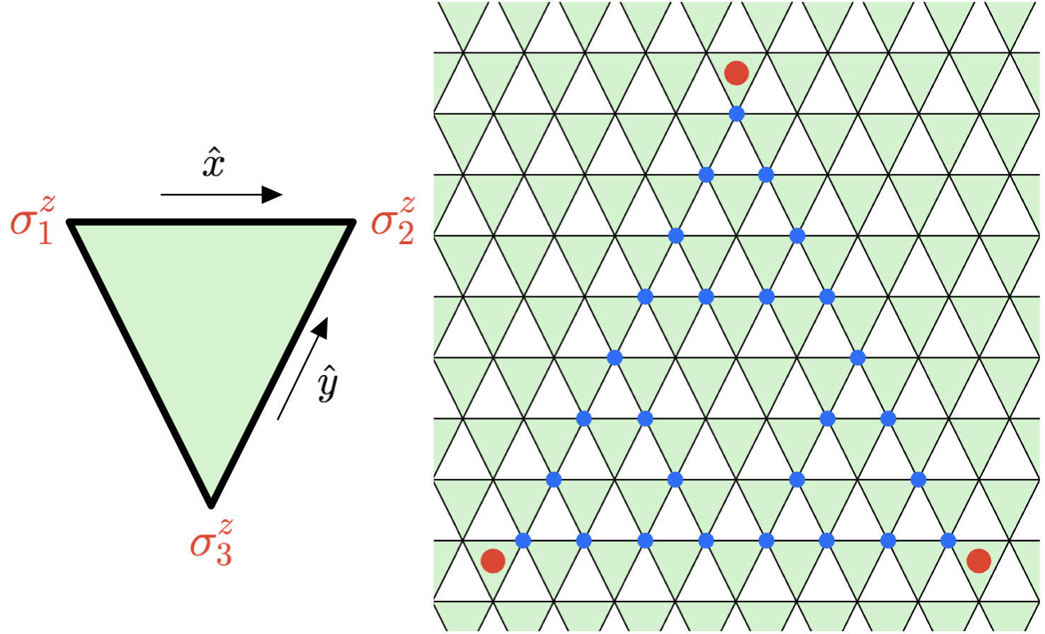
Figure 1: (Left): Three-body spin interaction on each downward facing triangle in Eq. 1. (Right): one of the low energy excitations of Eq. 1; starting with the obvious ground state with $\sigma^{z}=+1$, the spins are flipped to $\sigma^{z}=-1$ on a $\ell=3$ Sierpinski triangle (labelled blue), this configuration only costs energy on the unit triangles at the three corners (labelled red).

The Sierpinski triangle model Newman and Moore (1999); Yoshida (2013) is the paradigmatic model with fractal order. It is a classical statistical mechanical model for an Ising system on a triangular lattice whose Hamiltonian takes a simple form: one sums over all three-body interactions on downward facing unit triangles $\bigtriangledown$ as opposed to upward facing triangles $\triangle$ (Fig. 1):

$$H_{\mathrm{ST}}=\sum_{\bigtriangledown}-K\sigma^{z}_{1}\sigma^{z}_{2}\sigma^{z}_{3},$$ (1)

where the $\sigma^{z}=\pm 1$ are the Ising degrees of freedom placed at the vertices of each downward unit triangle. The low energy excited states of this model have a fractal structure: starting with the obvious ground state with uniform $\sigma^{z}_{j}=+1$, the low energy excited states correspond to flipping spins in the shape of a Sierpinski triangle, which does not cost energy anywhere except for the three corners of the Sierpinski triangle. If we view the corners of the Sierpinski triangle as point particles with finite energy, these particles cannot move along the lattice without creating more excitations that cost higher energy. Hence the mobility of these particles is highly restricted, and it is in this sense that they are fractons.

A quantum version of the Sierpinski triangle model was discussed in Ref. Vasiloiu et al. (2020); Zhou et al. (2021). Just like the classic quantum Ising model, the quantum Sierpinski triangle model has an extra transverse field

$$H_{q\mathrm{ST}}=\sum_{\bigtriangledown}-K\sigma^{z}_{1}\sigma^{z}_{2}\sigma^{z}_{3}-\sum_{j}h\sigma^{x}_{j}.$$ (2)

It was shown that the quantum Sierpinski triangle model has two highly desirable features:

(1) It is “self-dual”, meaning that under a duality transformation the $K$ and $h$ term will exchange. This self-duality is analogous to that of the Kramers-Wannier duality of the $1d$ quantum Ising model Kramers and Wannier (1941); Kogut (1979), and the self-duality of the quantum plaquette model on the square lattice Xu and Moore (2004). The self-duality implies that, if there were a quantum phase transition reached by tuning $h/K$ in Eq. 2, it must happen at $h=K$.

(2) Numerical simulation of the quantum Sierpinski triangle model suggests that the system may have a second order quantum phase transition at the self-dual point $h=K$ Zhou et al. (2021) (though earlier numerics suggested a first order transition Vasiloiu et al. (2020)); at the quantum phase transition, the energy density has a fractal dimension $d_{H}=\ln 3/\ln 2$ rather than scaling dimension 2 as in ordinary quantum phase transitions in $2d$ Zhou et al. (2021). This quantum phase transition is associated with the spontaneous breaking of a “fractal symmetry”; the phase with $h<K$ is identified as a “fractal order”, while the phase with $h>K$ is a disordered phase of the fractal symmetry (see the appendix for more discussion).

The nature of the quantum phase transition at $h=K$ in Eq. 2 is far from being understood, and the ordinary Landau-Ginzburg paradigm is no longer applicable. Numerics suggest that this transition is likely continuous, but many questions await answers. For example: is the continuous quantum phase transition stable against perturbations? For ordinary quantum phase transitions, this question is answered through the well-established renormalization group (RG) method Wilson (1971); Wilson and Fisher (1972); Wilson (1975), by evaluating the relevance or irrelevance of certain perturbations. But for the quantum phase transition under discussion, no reliable RG procedure has been established. Hence, key aspects of the transition must be explored experimentally. A tunable experimental realization of the classical and quantum Sierpinski triangle model would be extremely useful in understanding quantum phase transitions involving fractal geometry.

— Realizing the Sierpinski Triangle model with Rydberg atoms

The goal of this work is to describe a construction of both the classical and quantum Sierpinski triangle models from arrays of Rydberg atoms. To begin, let us consider a single atom for which we couple the ground state $|g\rangle$ and an excited Rydberg state $|r\rangle$ via a laser detuned from resonance. The two states coupled by the laser are the atom-field product states labelled $|g,N_{\gamma}+1\rangle$ and $|r,N_{\gamma}\rangle$, where $N_{\gamma}$ is the photon number of the laser so that $|g,N_{\gamma}+1\rangle$ has one extra photon compared to $|r,N_{\gamma}\rangle$. In the effective two-state problem, the Rabi frequency enters as a term coupling these two states. The simplest manifestation of the Rabi oscillations is as a term in the Hamiltonian $\Omega\sigma^{x}$ where $\sigma^{x}=|g,N_{\gamma}+1\rangle\langle r,N_{\gamma}|+|r,N_{\gamma}\rangle\langle g,N_{\gamma}+1|$.

If we blue-detune the laser from resonance, the energy gained by the atom being in the excited state $|r,N_{\gamma}\rangle$ relative to being in the state $|g,N_{\gamma}+1\rangle$ is $-\delta$, where $\delta$ is the detuning of the laser. This detuning then contributes a diagonal term to the effective Hamiltonian $-\delta\hat{n}$ where $\hat{n}$ is $0$ if the atom is in the state $|g,N_{\gamma}+1\rangle$ and $1$ if the atom is in the state $|r,N_{\gamma}\rangle$. This allows us to write down an effective two-state Hamiltonian in the basis of atom-field product states for the single atom

$$H_{1\text{ atom}}=\Omega\sigma^{x}-\delta\hat{n}.$$ (3)

Two atoms in $s-$orbital Rydberg states interact through a force that can be modelled by a Van der Waals potential $V(r)=C/r^{6}$ when the inter-atomic separation $r$ is large, where $C$ is a constant that scales very strongly with the principal quantum numbers of the two Rydberg states. For two identical Rydberg atoms with principal quantum number $n$ (not to be confused with the number operator $\hat{n}$), the coefficient $C$ of the Van der Waals interaction roughly scales with $\sim n^{11}$. In the remaining of the paper we will use the more detailed evaluation of the Van der Waals interaction given in Ref. Šibalić et al. (2017). As such, the total effective many-body Hamiltonian that describes a lattice of these atoms is

$$H=\sum_{i}\Omega_{i}\sigma^{x}_{i}+H_{0},\ \ H_{0}=-\sum_{i}\delta_{i}\hat{n}_{i}+\sum_{ij}V_{ij}\hat{n}_{i}\hat{n}_{j},$$ (4)

where $V_{ij}=C_{ij}/|i-j|^{6}$ and $i,j$ label the lattice sites.

We will start with the small Rabi frequency (relative to the detuning) limit of this model so that we may first ignore the $\sigma^{x}$ terms and focus on the classical part of the Hamiltonian $H_{0}$. To realize the classical Sierpinski triangle model of Eq. 1, we need to select the parameters in $H_{0}$ which yield low energy states that can be mapped to those of the Sierpinski triangle model. We consider the honeycomb lattice with two sublattices $\mathcal{A}$ and $\mathcal{B}$. We trap an “auxiliary” atom at each site in $\mathcal{A}$ and a “target” atom at each site in $\mathcal{B}$. An equivalent picture is that we take the triangular lattice and decorate each vertex with a target atom and the center of each downward facing triangle with an auxiliary atom (Fig. 2). We aim to reproduce the states of Eq. 1 only on the $\mathcal{B}$ sublattice with target atoms. The auxiliary atoms enlarge the Hilbert space and hence the states of model Eq. 1 with multi-spin interactions can be reproduced through two-body interactions only in the low energy subspace of the atomic system.

We assign different principal quantum numbers $n_{\mathcal{A}}$ and $n_{\mathcal{B}}$ for the Rydberg states of the auxiliary atoms located on sublattice $\mathcal{A}$ and target atoms on sublattice $\mathcal{B}$. Crucially, with a proper choice of $n_{\mathcal{A}}$, $n_{\mathcal{B}}$, as well as the detuning, the Hamiltonian $H_{0}$ can be organized as $H_{0}=\sum_{a\in\mathcal{A}}H_{0,a}$:

$$H_{0,a} = V\left(2\hat{n}_{a}+\hat{n}_{t,1}+\hat{n}_{t,2}+\hat{n}_{t,3}-2\right)^{2}+\sum_{i=1}^{3}v\hat{n}_{a}\hat{n}_{t,i}$$ (5)

$$\sim V\left(\sum_{i=1}^{3}4\hat{n}_{a}\hat{n}_{t,i}+\sum_{i<j}2\hat{n}_{t,i}\hat{n}_{t,j}-4\hat{n}_{a}-\sum_{i=1}^{3}3\hat{n}_{t,i}\right)$$ (7)

$$+ \sum_{i=1}^{3}v\hat{n}_{a}\hat{n}_{t,i}\cdots.$$ (9)

The sum $H_{0}=\sum_{a\in\mathcal{A}}H_{0,a}$ is over all sublattice sites $\mathcal{A}$, and each term in the sum involves an auxiliary atom ($\hat{n}_{a}=0,1$), as well as its three neighboring target atoms ($\hat{n}_{t,i}=0,1$) which form a downwards facing triangle on the honeycomb lattice. The second line of Eq. 9 uses the fact that $\hat{n}_{a}^{2}=\hat{n}_{a}$, $\hat{n}_{t}^{2}=\hat{n}_{t}$ for $\hat{n}=0,1$. $H_{0}$ contains a two-body repulsive interaction $V_{\mathcal{A}\mathcal{B}}=4V+v$ between the auxiliary atom and its neighboring target atoms, as well as a repulsive interaction $V_{\mathcal{B}\mathcal{B}}=2V$ between two nearest neighbor target atoms (Fig. 2).

When $v>0$, there are two classes of configurations of $(\hat{n}_{t,i};\ \hat{n}_{a})$ on each downward triangle, both of which are the ground states of $H_{0}$:

$$(1)\ \ \hat{n}_{a}=1,\ \hat{n}_{t,i}=0;$$ (10)

$$\mathrm{or} (2)\ \ \hat{n}_{a}=0,\ \text{two of }\hat{n}_{t,i}=1.$$ (12)

As a comparison, the ground states of the classical Sierpinski triangle model $H_{\mathrm{ST}}$ also have two types of ground states on each downwards facing triangle:

$$(1)\ \ \sigma^{z}_{1}=\sigma^{z}_{2}=\sigma^{z}_{3}=+1;$$ (13)

$$\mathrm{or} (2)\ \ \text{Two of }\sigma^{z}_{i}=-1.$$ (15)

Now the ground states of $H_{0}$ can be one-to-one mapped to the ground states of the classical Sierpinski triangle model, as long as we identify $\sigma^{z}_{i}=1-2\hat{n}_{t,i}$. In fact in the appendix we will show that, all the states of Eq. 1 (ground and excited states) can be mapped one-to-one to the low energy subspace of $H_{0}$ when $v>0$.

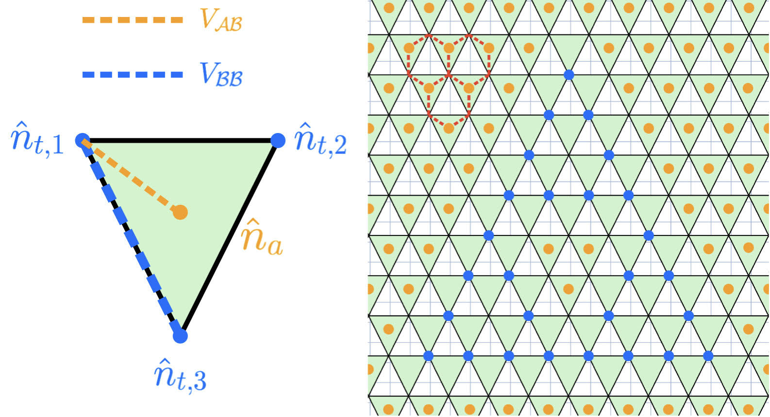
Figure 2: We trap atoms on both the vertices and the center of each downward triangle of a triangular lattice, which together form a honeycomb lattice (three hexagons of the honeycomb lattice are shown in the figure). The atoms on the vertices and the triangle centers are the “target” and “auxiliary atoms” respectively. The Hamiltonian Eq. 9 reduces to $V_{\mathcal{A}\mathcal{B}}=4V+v$ between a auxiliary atom and its neighboring target atoms, and interaction $V_{\mathcal{B}\mathcal{B}}=2V$ between two neighboring target atoms. The ground state of Eq. 9 demands that, on each downward facing triangle, either $\hat{n}_{a}=1$ (labelled orange) and all $\hat{n}_{t}=0$; or $\hat{n}_{a}=0$ and two out of three $\hat{n}_{t}=1$ (labelled blue).

The relation between $V_{\mathcal{A}\mathcal{B}}$ and $V_{\mathcal{B}\mathcal{B}}$ can be tuned by choosing the principal quantum numbers $n_{\mathcal{A}}$ and $n_{\mathcal{B}}$ properly. For example, for potassium atoms, if we choose $n_{\mathcal{A}}=76$ and $n_{\mathcal{B}}=113$, then using the techniques in Ref. Šibalić et al. (2017) and the fact that the interatomic distances are related by $r_{\mathcal{B}\mathcal{B}}=\sqrt{3}r_{\mathcal{A}\mathcal{B}}$, we found that both interactions are repulsive and satisfy $V_{\mathcal{A}\mathcal{B}}/V_{\mathcal{B}\mathcal{B}}\sim 2.628$ ($v\sim 1.26V$). Note that different choices are possible; our results apply more broadly than just to this specific choice of atom and principal quantum numbers.

In the real system, there are perturbations to Eq. 9. These include other terms induced by the Van der Waals interaction, for example the repulsion between Rydberg states on two neighboring auxiliary atoms, whose strength $V_{\mathcal{A}\mathcal{A}}$ compared with $V_{\mathcal{B}\mathcal{B}}$ is $V_{\mathcal{A}\mathcal{A}}/V_{\mathcal{B}\mathcal{B}}\sim 0.011$ using the example principal quantum numbers we chose above. The repulsion $V_{\mathcal{B}\mathcal{B}}^{\prime}$ between the target atoms on two second neighbor $\mathcal{B}$ sites is also much weaker than $V_{\mathcal{B}\mathcal{B}}$ due to the rapid decay of the Van der Waals interaction with distance. Another notable perturbation is the interaction $V^{\prime}_{\mathcal{A}\mathcal{B}}$ between an auxiliary atom and its next-neighbor target atom. Compared with $V_{\mathcal{B}\mathcal{B}}$, the two perturbations $V_{\mathcal{B}\mathcal{B}}^{\prime}$ and $V^{\prime}_{\mathcal{A}\mathcal{B}}$ are

$$\frac{V^{\prime}_{\mathcal{B}\mathcal{B}}}{V_{\mathcal{B}\mathcal{B}}}=\frac{1}{(\sqrt{3})^{6}}\sim 0.037,\ \ \frac{V^{\prime}_{\mathcal{A}\mathcal{B}}}{V_{\mathcal{B}\mathcal{B}}}=\frac{1}{2^{6}}\frac{V_{\mathcal{A}\mathcal{B}}}{V_{\mathcal{B}\mathcal{B}}}\sim 0.041.$$ (16)

These perturbations shift the energy of the excited state of the Sierpinski triangle shape. Let us consider an excited state with flipped “spins” ($\hat{n}_{t}=1$) on a Sierpinski triangle with side length $L=2^{\ell}$. In the ideal model of Eq. 1, the energy of this excited state does not depend on $L$ or $\ell$: all the energy cost arises from the corners of the Sierpinski triangle and the energy compared with the ground state is $E_{\text{ex}}=E-E_{g}=6K=3V=3/2\times V_{\mathcal{B}\mathcal{B}}$. However, in the real system the leading order perturbations $V_{\mathcal{A}\mathcal{B}}^{\prime},V_{\mathcal{A}\mathcal{A}}$ and $V_{\mathcal{B}\mathcal{B}}^{\prime}$ cause the energy cost of creating a Sierpinski triangle to scale with its size. In particular, the energy of the excitation relative to the ground state with uniform $\hat{n}_{a}=1$ and $\hat{n}_{t}=0$ is estimated to be (details are given in the appendix)

$$E_{\text{ex}}^{\text{Ry}}=(3/2-0.1+0.47\times 3^{\ell-3})V_{\mathcal{B}\mathcal{B}}$$ (17)

for Sierpinski triangles of $\ell\geq 2$. Since the actual energy cost of creating a Sierpinski triangle increases with the size of the triangle, the perturbations can no longer be ignored for large enough Sierpinski triangles. Finite-size fractal excitations, however, will still be observable.

— Experimental Proposals

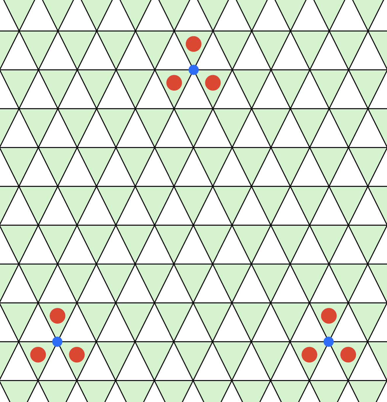
Figure 3: With Hamiltonian Eq. 9, if three target atoms at the corners of a triangle with side length $L=8$ are excited from the ground state to the Rydberg state, it costs energy $3V+3v$ at each corner. If we apply an extra detuning $-\bar{\delta}_{\mathrm{C}}\hat{n}_{t}$ on the three corners of the triangle, for sufficiently large $\bar{\delta}_{\mathrm{C}}$ the ground state of the system is given by the fractal configuration in Fig. 1.

Next, we outline a procedure to enable experimental observation of a spontaneously generated fractal-shaped excitation. This can be done by adiabatically evolving a prepared ground state of Eq. 9 to the Sierpinski triangle excitation, which is the ground-state of a new Hamiltonian achieved by slowly and carefully varying the detuning and Rabi frequency. Note that this procedure requires a level of local control beyond that present in most current Rydberg experimental platforms, but the elements of which have been demonstrated experimentally Labuhn et al. (2014). We start with the Hamiltonian of Eq. 9 with a small and finite Rabi frequency. To ensure a unique ground state (to enable an adiabatic evolution), we first deform Eq. 9 with a small extra detuning $\bar{\delta}\hat{n}_{t}$ on all target atoms outside of a triangle with side $L=2^{\ell}$. We then prepare an initial state with all target atoms $\hat{n}_{t}=0$ and $\hat{n}_{a}=1$, which is equivalent to $\sigma^{z}=1$ uniformly in Eq. 1 and represents the unique ground state of the Hamiltonian prepared above. We slowly deform the Hamiltonian with time-dependent Rabi frequency $\Omega(t)$ and detuning $\delta_{i}(t)$ within the triangle, reaching the final Hamiltonian with extra detuning $-\bar{\delta}_{\mathrm{C}}\hat{n}_{t}$ localized to three target atoms at the corners of the triangle (Fig. 3). With sufficiently large $\bar{\delta}_{\mathrm{C}}$, the unique ground state of the final Hamiltonian contains a Sierpinski triangle arrangement of all the atoms inside the triangle, as shown in Fig. 1 and Fig. 2, despite the fact that the extra detuning $-\bar{\delta}_{\mathrm{C}}\hat{n}_{t}$ is only applied locally at the corners rather than throughout the entire interior. Based on our estimate of energy in Eq. 17 which includes further leading neighbor interactions arising from the Van der Waals interaction, this phenomenon can hold up to Sierpinski triangles with $\ell=4$ (side length $L=16$, containing 81 atoms), as a single Sierpinski triangle configuration still has lower energy than fragmented configurations.

We have specified the initial and final Hamiltonian for the desired evolution; an adiabatic path of the detuning and Rabi frequency for observing Ising-like crystallization of Rydberg atoms has already been demonstrated Schauß et al. (2015); browaeys2daf; lukinphases. Leveraging the aforementioned power of local control, we could also create arbitrary configurations of the Rydberg array, including the Sierpinski triangle. Spectroscopic measurement of the energy of the Sierpinski configuration compared with that of fragmented configurations could then confirm that it represents a low-lying excited state. This technique would no longer rely on adiabatic evolution.

This experimental platform also gives us the potential to probe quantum phase transitions by controlling the Rabi frequency. When the Rabi frequency $\Omega$ is increased uniformly on all the target atoms, around $\Omega\sim V$ there is expected to be a quantum phase transition similar to the one recently studied numerically Vasiloiu et al. (2020); Zhou et al. (2021). In the large $\Omega$ phase, one is not supposed to observe the fractal configuration in the proposed experiment above, i.e. the configuration of Fig. 3 will not evolve to the one in Fig. 1 and Fig. 2. As we pointed out before, the nature of this transition is far from being understood. Hence the realization of the quantum phase transition in experimental systems with high tunability is crucial to understand these exotic quantum phase transitions, and to test possible theoretical paradigms developed in the future.

The fractal structure of the fractal orders also manifests at the level of the correlation functions. In both the classical and quantum Sierpinski triangle models, the three-point correlation function $\mathcal{C}_{3}=\langle\sigma^{z}_{j}\sigma^{z}_{j+L\hat{x}}\sigma^{z}_{j+L(\hat{x}-\hat{y})}\rangle$ is a characteristic quantity which plays the role of the correlation function of ordinary quantum many-body systems. The three-point correlation decays hyper-exponentially with the Hausdorff dimension at finite temperature Yoshida (2013); Newman and Moore (1999) and its scaling at the quantum critical point $h=K$ was computed in Ref. Zhou et al. (2021). In the experimental realization of Eq. 9, the three-point correlation function $\mathcal{C}_{3}$ can be reconstructed by averaging over multiple single-site resolution snapshots of the configuration of the target atoms taken in separate experimental realizations. Similar techniques have been used previously in cold-atom experiments to reconstruct quantities such as the spin correlation functions in Fermi-Hubbard systems Parsons et al. (2016); Endres et al. (2011). Experimental measurement of $\mathcal{C}_{3}$, whose scaling with distance diagnoses the fractal physics of the model, will be crucial in understanding the nature of this quantum phase transition.

— Discussion

Previous proposals for realizing fracton related states mostly focused on states that are analogous to type-I fractons Xu and Fisher (2007); Pretko (2019); Sous and Pretko (2020); Giergiel et al. (2021). For example, theoretical efforts on constructing fracton related states were made based on localized Majorana zero modes for both type-I and type-II states Xu and Fu (2010); You and von Oppen (2019). Compared with previous proposals, the platform of Rydberg atoms discussed in the current work is highly tunable with precision at the level of a single atom. Another advantage of the platform of Rydberg atoms, and in general cold atom systems, is fast manipulation of parameters in the Hamiltonian, which can either periodically drive the system, or cause a quantum quench Polkovnikov et al. (2011); Wintersperger et al. (2020); Potirniche et al. (2017); Singh et al. (2019); Chen et al. (2019); Bluvstein et al. (2021); Keesling et al. (2019); Bernien et al. (2017). Many exotic features are expected in the quantum dynamics of fracton related models due to the restricted motion of the fracton excitations Pai and Pretko (2019); Prem et al. (2017); Feldmeier et al. (2020); Kim and Haah (2016). By quickly tuning parameters such as the Rabi frequency in Eq. 4, one can compare the quantum dynamics of the fractal order simulated with Rydberg atoms with future analytical and numerical analysis. Furthermore, our construction of Eq. 9 used to reproduce multi-spin interactions in Rydberg Hamiltonians with only two-body interactions but an enlarged Hilbert space, can be extended to fracton related models richer than the Sierpinski triangle model. One example of such extension is given in the appendix.

The authors thank Chao-Ming Jian and Hannes Bernien for very helpful discussions. C.X. is supported by NSF Grant No. DMR-1920434, and the Simons Investigator program. D.W. acknowledges support from the Army Research Office (MURI W911NF1710323), and the University of California Multicampus Research Programs and Initiatives (MRP19-601445). We gratefully acknowledge support via the UC Santa Barbara NSF Quantum Foundry funded via the Q-AMASE-i program under award DMR-1906325. This material is based upon work supported by the U.S. Department of Energy, Office of Science, National Quantum Information Science Research Centers, Quantum Science Center.

Appendix A Estimate of energy of Sierpinski triangle excitation in real system

With the inclusion of the perturbations of $V_{\mathcal{AA}},V_{\mathcal{BB}}^{\prime}$ and $V_{\mathcal{AB}}^{\prime}$, we can calculate the relative cost of creating a Sierpinski triangle excited state by exciting target atoms and de-exciting auxiliary atoms in the perturbed ground state with $\hat{n}_{a}=1$ and $\hat{n}_{t}=0$ uniformly. For a Sierpinski triangle of length $L=2^{\ell}$, the energy cost $E_{\text{ex}}^{\text{Ry}}$ is

$$E_{\text{ex}}^{\text{Ry}}=3V+N^{\prime}_{\mathcal{BB}}V_{\mathcal{BB}}^{\prime}+N^{\prime}_{\mathcal{AB}}V_{\mathcal{AB}}^{\prime}-N_{\mathcal{AA}}V_{\mathcal{AA}},$$ (18)

where $N^{\prime}_{\mathcal{BB}}$, $N^{\prime}_{\mathcal{AB}}$ and $N_{\mathcal{AA}}$ are the number of interactions $V_{\mathcal{BB}}^{\prime}$, $V_{\mathcal{AB}}^{\prime}$ we have turned on, and the number of interactions $V_{\mathcal{AA}}$ we have turned off, respectively, in order to create the Sierpinski triangle.

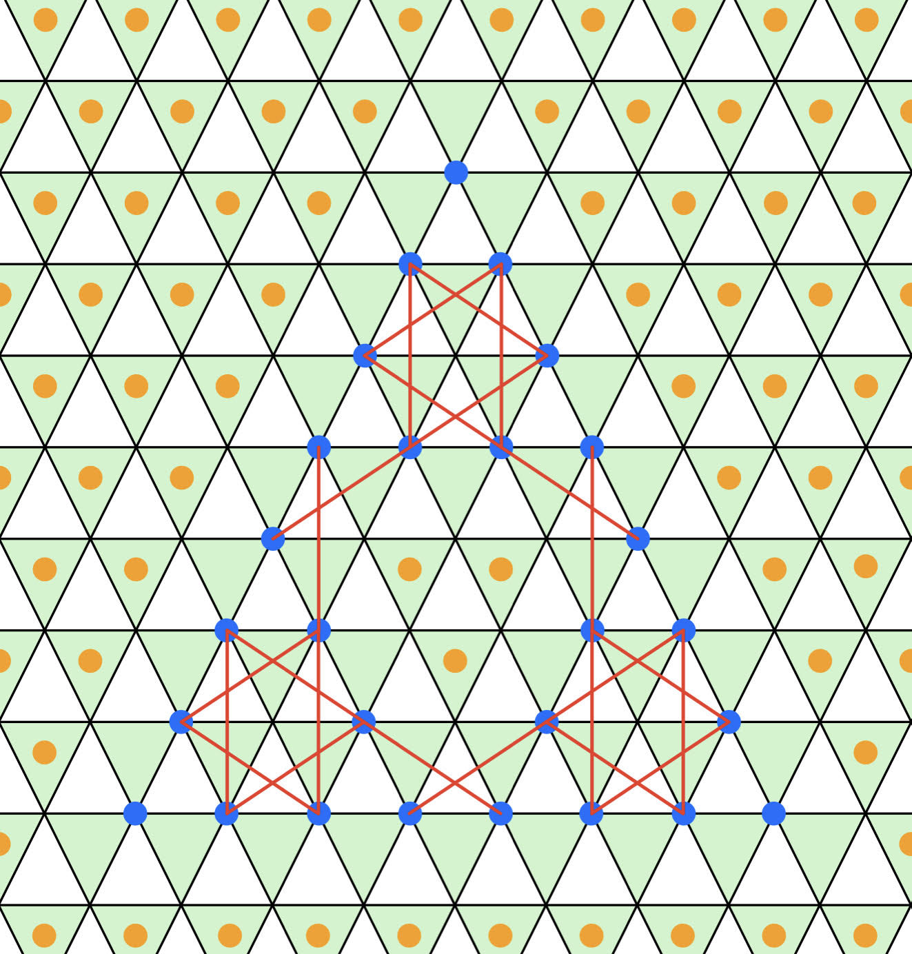
Figure 4: The next neighbor Van der Waals interaction between target atoms.

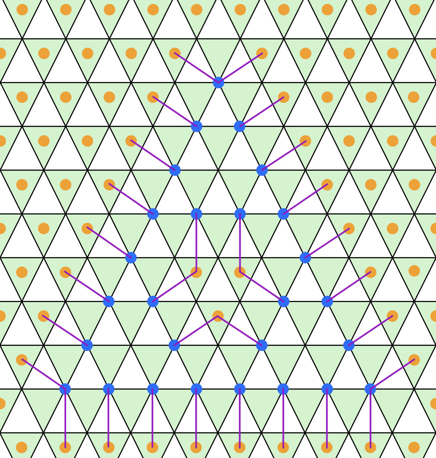
Figure 5: The next neighbor interaction between auxiliary atoms and target atoms.

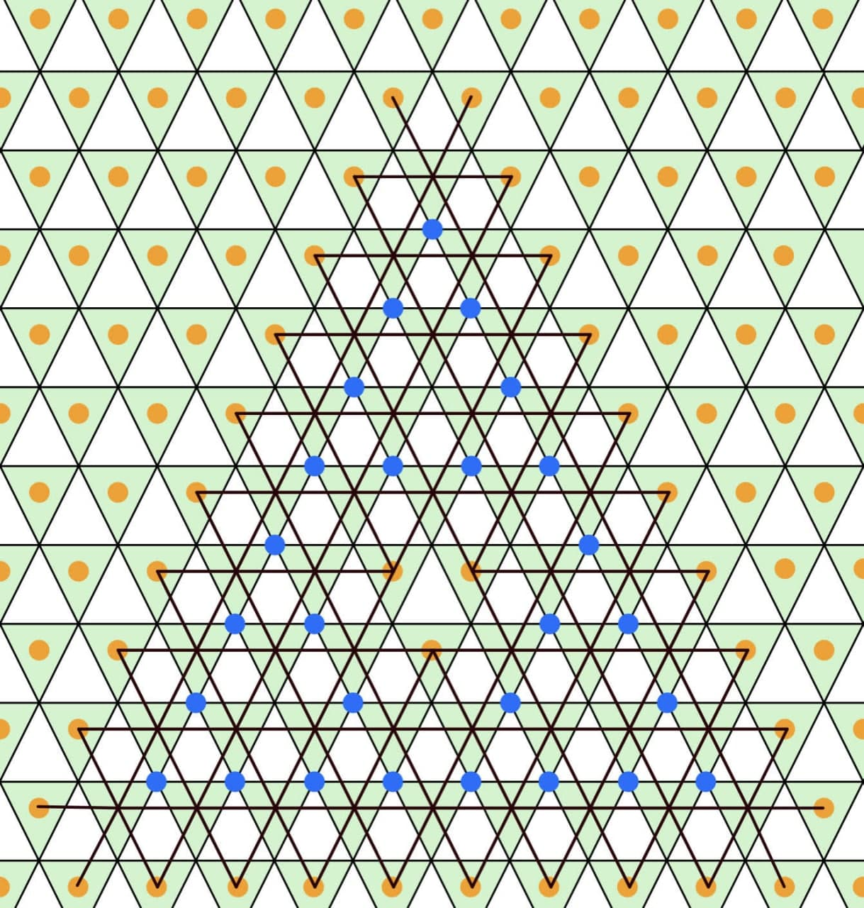
Figure 6: The nearest neighbor interaction between auxiliary atoms that are “lost” while creating the Sierpinski triangle excitation.

Here $N_{\mathcal{BB}}^{\prime}$ as a function of $\ell$ is

$$N^{\prime}_{\mathcal{BB}}(\ell)=(3^{\ell}-3)\text{ for }\ell\geq 2.$$ (19)

This result can be seen from the following: each Sierpinski triangle of length $2^{\ell-1}$ has a corresponding number of $V_{\mathcal{BB}}^{\prime}$ interactions $N^{\prime}_{\mathcal{BB}}(\ell-1)$. The Sierpinski triangle of length $2^{\ell}$ is constructed by gluing three copies of of the smaller Sierpinski triangle of length $2^{\ell-1}$ together at the corners so that it has $3N^{\prime}_{\mathcal{BB}}(\ell-1)$ many interactions, as well as the added interactions between target atoms belonging to different smaller Sierpinski triangles (Fig. 4). Including these added interactions, of which there are $6$, we recover a recurrence relation for $N^{\prime}_{\mathcal{BB}}(\ell)$:

$$N^{\prime}_{\mathcal{BB}}(\ell)=3N^{\prime}_{\mathcal{BB}}(\ell-1)+6$$

with the number of interactions for the $\ell=2$ Sierpinski triangle as the initial condition, $N^{\prime}_{\mathcal{BB}}(2)=6$. This recurrence relation can be solved for

$$N^{\prime}_{\mathcal{BB}}(\ell)=(3^{\ell}-3)\text{ for }\ell\geq 2,$$

which is the stated result.

We can compute the number of $V_{\mathcal{AB}}^{\prime}$ interactions that we have turned on in a similar manner. The total number of these interactions is

$$N^{\prime}_{\mathcal{AB}}(\ell)=(3^{\ell}+3)\text{ for }\ell\geq 2.$$

Since these are interactions between auxiliary atoms and target atoms, these occur between the target atoms on the edges of the Sierpinski triangle and surrounding auxiliary atoms, as well as between target atoms and the auxiliary atoms in the interior of the Sierpinski triangle. For a Sierpinski triangle of length $L=2^{\ell}$, the total number of interactions coming from the target atoms at the edges is $3L=3\times 2^{\ell}$. Counting the interactions coming from the interior of the Sierpinski triangle $N_{\mathcal{AB}}^{\text{int}}(\ell)$ is more complicated as it depends on the length of the previous iteration of the Sierpinski triangle. These can be counted as the contribution from the largest missing triangle $3\times(2^{\ell-1}-2)$, plus three times the number of interactions from the last iteration $3N_{\mathcal{AB}}^{\text{int}}(\ell-1)$. As a result, we are yet again left with a recurrence relation

$$N_{\mathcal{AB}}^{\text{int}}(\ell)=3N_{\mathcal{AB}}^{\text{int}}(\ell-1)+3\times(2^{\ell-1}-2)$$

with initial condition $N_{\mathcal{AB}}^{\text{int}}(2)=0$. This can be solved for

$$N_{\mathcal{AB}}^{\text{int}}=3^{\ell}-3\times 2^{\ell}+3.$$

Therefore the total number of $V_{\mathcal{AB}}^{\prime}$ interactions we have turned on is

$$N_{\mathcal{AB}} =N_{\mathcal{AB}}^{\text{int}}+3\times 2^{\ell},$$

$$=(3^{\ell}+3)\text{ for }\ell\geq 2.$$

The calculation of the number of $V_{\mathcal{AA}}$ interactions lost when creating the Sierpinski triangle excitation is nearly identical to the previous calculation. The total number of lost interactions can be calculated as

$$N_{\mathcal{AA}}=\frac{1}{2}(11\times 3^{\ell}+21)\text{ for }\ell\geq 2.$$ (20)

There are three sources of the loss of $V_{\mathcal{AA}}$ interactions: 1) the loss of interaction between two de-excited auxiliary atoms in downwards triangles in the Sierpinski triangle, 2) the loss of interaction between a de-excited auxiliary atom on the edges and corners of the Sierpinski triangle and an excited auxiliary atom surrounding the Sierpinski triangle and 3) the loss of interaction between a de-excited auxiliary atom in the Sierpinski triangle and an excited auxiliary atom in the interior of the Sierpinski triangle.

The contribution to the total number of lost $V_{\mathcal{AA}}$ interactions from the first two cases 1) and 2) can be found to be $\frac{1}{2}(7\times 3^{\ell}-3)+6(2^{\ell}+1)$. There are an additional $12$ lost interactions that come from de-excited auxiliary atoms at the corners of the Sierpinski triangle and do not scale with $\ell$. For the $\ell=2$ Sierpinski triangle there are $N_{\mathcal{AA}}^{1)}(2)=30$ lost interactions not including the ones from the edges and corners. Gluing these triangles to generate a $\ell=3$ Sierpinski triangle gives us $3$ times as many interactions as well as an additional $3$ lost interactions between auxiliary atoms belonging to different smaller Sierpinski triangles. Hence we are left with a recursion relation

$$N^{1)}_{\mathcal{AA}}(\ell)=3N^{1)}_{\mathcal{AA}}(\ell-1)+3.$$

Using $N_{\mathcal{AA}}^{1)}(2)=30$ as the initial condition, we have a solution of

$$N_{\mathcal{AA}}^{1)}(\ell)=\frac{1}{2}(7\times 3^{\ell}-3)\text{ for }\ell\geq 2.$$

$N_{\mathcal{AA}}^{2)}$ is straightforward: $N_{\mathcal{AA}}^{2)}=6(2^{\ell}-1)+12=6(2^{\ell}+1)$ including the interactions at the corners. Hence, restoring the additional $12$ interactions, $N_{\mathcal{AA}}^{1)}+N_{\mathcal{AA}}^{2)}=\frac{1}{2}(7\times 3^{\ell}-3)+6(2^{\ell}+1)$.

We recover another recurrence relation for the number of lost interactions in the interior for case 3):

$$N_{\mathcal{AA}}^{3)}(\ell)=3N_{\mathcal{AA}}^{3)}(\ell-1)+6\times(2^{\ell-1}-2)$$

with initial condition $N_{\mathcal{AA}}^{3)}(2)=0$. This can be solved for

$$N_{\mathcal{AA}}^{3)}(\ell)=2\times 3^{\ell}-3\times 2^{\ell+1}+6.$$

The total number of lost $V_{\mathcal{AA}}$ interactions is then

$$N_{\mathcal{AA}} =N_{\mathcal{AA}}^{3)}(\ell)+\frac{1}{2}(7\times 3^{\ell}-3)+6(2^{\ell}+1),$$

$$=\frac{1}{2}(11\times 3^{\ell}+21)\text{ for }\ell\geq 2.$$

Combining all the perturbations evaluated above, $E_{\text{ex}}^{\text{Ry}}$ is given by

$$E_{\text{ex}}^{\text{Ry}} =3V+N^{\prime}_{\mathcal{BB}}V_{\mathcal{BB}}^{\prime}+N^{\prime}_{\mathcal{AB}}V_{\mathcal{AB}}^{\prime}-N_{\mathcal{AA}}V_{\mathcal{AA}},$$ (21)

$$\approx(3/2-0.1+0.47\times 3^{\ell-3})V_{\mathcal{BB}}.$$ (23)

Appendix B Mapping between states

On a unit downward facing triangle, the mapping between states in Eq. 1 and the states in Eq. 9 is:

$$\sigma^{z}=(+1,+1,+1),\ \ \mathrm{Energy}=-K$$ (24)

$$\rightarrow (\hat{n}_{t,i};\hat{n}_{a})=(0,0,0;1),\ \ \mathrm{Energy}=0;$$ (28)

$$\sigma^{z}=(-1,-1,+1),\ \ \mathrm{Energy}=-K,$$

$$\rightarrow (\hat{n}_{t,i};\hat{n}_{a})=(1,1,0;0),\ \ \mathrm{Energy}=0;$$ (32)

$$\sigma^{z}=(-1,+1,+1),\ \ \mathrm{Energy}=+K,$$

$$\rightarrow (\hat{n}_{t,i};\hat{n}_{a})=(1,0,0;0),\ \ \mathrm{Energy}=V;$$ (36)

$$\sigma^{z}=(-1,-1,-1),\ \ \mathrm{Energy}=+K$$

$$\rightarrow (\hat{n}_{t,i};\hat{n}_{a})=(1,1,1;0),\ \ \mathrm{Energy}=V.$$ (38)

The Hilbert space of the atoms is bigger than the one of the spins; hence there are some extra states with even higher energy. The $v\hat{n}_{a}\hat{n}_{t,i}$ term in $H_{0}$ does not affect the energy of the states list above, but they will separate the other states in the atomic Hilbert space with extra energy cost:

$$(\hat{n}_{t,i};\hat{n}_{a})=(1,0,0;1),\ \ \mathrm{Energy}=V+v;$$ (39)

(40)

$$(\hat{n}_{t,i};\ \hat{n}_{a})=(1,1,0;1),\ \ \mathrm{Energy}=4V+2v;$$ (41)

(42)

$$(\hat{n}_{t,i};\ \hat{n}_{a})=(1,1,1;1),\ \ \mathrm{Energy}=9V+3v;$$ (43)

(44)

$$(\hat{n}_{t,i};\ \hat{n}_{a})=(0,0,0;0),\ \ \mathrm{Energy}=4V.$$ (45)

Hence with positive $v$, the low energy states of the Rydberg atom systems can be exactly mapped to the states of the Ising spins in Eq. 9, with $V=2K$.

Appendix C Fractal symmetry in the quantum Sierpinski triangle model

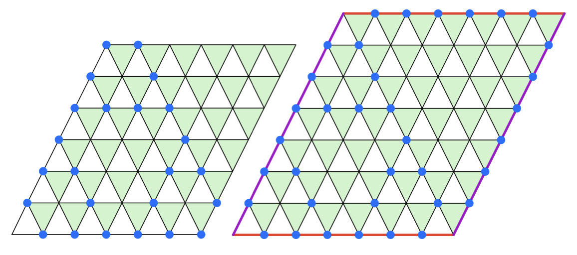
Figure 7: (Left): when the system is defined on a triangular lattice with periodic boundary conditions, and $L_{x}=L_{y}=2^{k}-1$ ($k=3$ in the figure), there exist symmetry generation operators $\hat{G}(\mathcal{L})=\prod_{j\in\mathcal{L}}\sigma^{x}_{j}$ where $\mathcal{L}$ are all the sites labeled in blue. (Right): we duplicate the bottom row on the top, and the left column on the right of the lattice to demonstrate the periodic boundary conditions.

For a quantum system to have a symmetry, the Hamiltonian of the system needs to commute with a symmetry generation operator $\hat{G}$. For example, the standard quantum Ising model $H=\sum_{\langle i,j\rangle}-K\sigma^{z}_{i}\sigma^{z}_{j}-\sum_{j}h\sigma^{x}_{j}$ has a $Z_{2}$ spin symmetry that is generated by the operator $\hat{G}=\prod_{j}\sigma^{x}_{j}$ which commutes with the entire Hamiltonian. Although the Hamiltonian has $Z_{2}$ spin symmetry, in the Ising ordered phase with $K\gg h$, (at least in a certain basis) the ground state wave function of the system in the thermodynamics limit is not invariant under the operation of $\hat{G}$. The ground states are degenerate in the ordered phase, and $\hat{G}$ would take one ground state to another. In this sense, the $Z_{2}$ symmetry is spontaneously broken in the Ising ordered phase. On the other hand, in the Ising disordered phase $h\gg K$ the $Z_{2}$ symmetry is preserved,i.e. the ground state wave function is unique and invariant under operation of $\hat{G}$.

In the quantum Sierpinski triangle model Eq. 2, let us consider periodic boundary conditions for convenience. The Hamiltonian does not have exact subsystem symmetry for most system sizes; however, when the system is a parallelogram with side length $L_{x}=L_{y}=2^{k}-1$ and $k$ being a positive integer, there exists a series of symmetry generation operators $\hat{G}(\mathcal{L})$ which are a product of $\sigma^{x}_{j}$ on a subset of the lattice that belong to a Sierpinski triangle:

$$\hat{G}(\mathcal{L})=\prod_{j\in\mathcal{L}}\sigma_{j}^{x}.$$ (46)

The shape of $\mathcal{L}$ is illustrated in Fig. 7. Notice that due to the subtlety of the periodic boundary conditions, $\hat{G}(\mathcal{L})$ commutes with the entire Hamiltonian when and only when the system size $L_{x}=L_{y}=2^{k}-1$. And when $K>h$, in the thermodynamics limit $(k\rightarrow\infty)$ the system has many degenerate ground states which are not invariant under the operation of $\hat{G}(\mathcal{L})$, hence the phase $K>h$ spontaneously breaks the fractal symmetry generated by $\hat{G}(\mathcal{L})$. While in the phase $h>K$ the ground state is unique and invariant under operation of $\hat{G}(\mathcal{L})$.

Appendix D The Sierpinski tetrahedron model

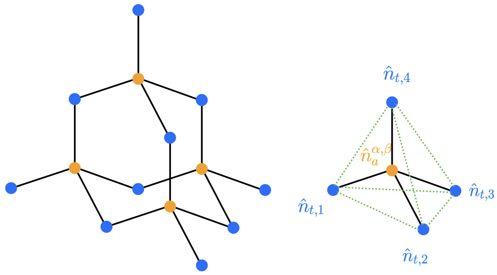
Figure 8: The diamond lattice constructed out of tetrahedra with target atoms $\hat{n}_{t,1},\dots,\hat{n}_{t,4}$ decorating the vertices and auxiliary atoms supporting two different quantum numbers $\hat{n}_{a}^{\alpha,\beta}$ decorating the centers.

One of the main obstacles in constructing many exotic states of matter considered theoretically is the multi-spin interaction in the Hamiltonian. Our platform constructed with Rydberg atoms can simulate much of the low energy physics of the Sierpinski triangle model, which originally involves three-body interactions. In fact, our construction can be expanded to other fractal models with more general multi-spin interactions as well. An example of such a model that we might hope to realize is the natural extension of the Sierpinski triangle model to three-dimensions: the Sierpinski tetrahedron model Garrahan (2002); Devakul et al. (2019). To construct this model, we first glue tetrahedra with effective spin-$1/2$ degrees of freedom $(\sigma^{z}=\pm 1)$ at the vertices together at the corners to form a lattice. As each tetrahedron has four vertices, one may sum over all four-body interactions on each tetrahedron,

$$H_{\text{tetra}}=\sum_{\text{tetra}}-K\sigma_{1}^{z}\sigma_{2}^{z}\sigma_{3}^{z}\sigma_{4}^{z}.$$ (47)

Many of the technical features of this model are similar to those of the Sierpinski triangle model of Eq. 1:

(1) The low energy excitations above the ground state are created at the corners of a Sierpinski tetrahedron (a self-similar fractal with Hausdorff dimension $d_{H}=2$) of flipped spins and are fractons.

(2) The quantum model with an added transverse field $\sum_{j}-h\sigma^{x}_{h}$ is self-dual and there is a fractal symmetry that is spontaneously broken in the phase $K>h$. A quantum phase transition is expected at $h=K$, although the nature of the transition needs further study.

Fractal-ordered phases such as the Sierpinski triangle and Sierpinski tetrahedron models tend to have their fractal structure manifest at the level of the correlation functions. In the Sierpinski triangle model, the three-point correlation function $\mathcal{C}_{3}=\langle\sigma^{z}_{j}\sigma^{z}_{j+L\hat{x}}\sigma^{z}_{j+L(\hat{x}-\hat{y})}\rangle$ is known to be non-vanishing only when $L=2^{\ell}$ and decays hyper-exponentially with the Hausdorff dimension at finite temperature Yoshida (2013); Newman and Moore (1999).

In the Sierpinski tetrahedron model, the four-point correlation function $\mathcal{C}_{4}=\langle\sigma^{z}_{j}\sigma^{z}_{j+L\hat{x}}\sigma^{z}_{j+L\hat{y}}\sigma^{z}_{j+L\hat{z}}\rangle$ displays the same smoking-gun signatures of fractal order as $\mathcal{C}_{3}$ in the Sierpinski triangle model. This correlation function may be computed in a similar fashion as one might compute the two-point correlation function of the $1d$ Ising model, $\langle\sigma^{z}_{j}\sigma^{z}_{j+L}\rangle$. Since there is a one-to-one correspondence between tetrahedra and vertices, we define new spin-1/2 variables at the center of each tetrahedron $\tau^{z}_{T}=(\sigma^{z}_{1}\sigma^{z}_{2}\sigma^{z}_{3}\sigma^{z}_{4})$. The Hamiltonian now describes a collection of statistically independent spin variables $\tau_{T}$,

$$H_{\text{tetra,d}}=\sum_{T\in\text{tetra}}-K\tau_{T}.$$ (48)

Since the $\tau$ variables are independent from one another, the correlations of products of $\tau$’s factor nicely such that

$$\bigg{\langle}\prod_{j}\tau_{j}\bigg{\rangle} = \prod_{j}\langle\tau_{j}\rangle,$$ (49)

$$= \prod_{j}\frac{\sum_{\{\tau\}}\tau_{j}e^{\beta K\sum_{T}\tau_{T}}}{\sum_{\{\tau\}}e^{\beta K\sum_{T}\tau_{T}}},$$ (51)

$$= \prod_{j}\bigg{(}\frac{e^{\beta K}-e^{-\beta K}}{e^{\beta K}+e^{-\beta K}}\bigg{)},$$ (53)

$$= \tanh(\beta K)^{\#\text{ of }\tau\text{'s}}.$$ (55)

Taking products of spins over a Sierpinski tetrahedron of length $L=2^{\ell}$ for integer $\ell$ allows us to write the four-point correlation as

$$\mathcal{C}_{4} = \bigg{\langle}\prod_{j\in\text{ST}(L)}\tau_{j}\bigg{\rangle},$$ (56)

$$= \tanh(\beta K)^{\#\text{ of tetrahedra}},$$ (58)

$$= \tanh(\beta K)^{L^{2}}.$$ (60)

The four point correlations for $L\neq 2^{\ell}$ must vanish.

The approach we have taken in realizing the Sierpinski triangle model in Eq. 9 can be extended to this Sierpinski tetrahedron model with a four-body interaction. Starting from the diamond lattice, we decorate each vertex and center of every tetrahedron with target atoms and an auxiliary atom respectively as shown in Fig. 8. We couple the auxiliary atom to two different Rydberg states using lasers with different frequencies, and the two Rydberg states are labelled by their principal quantum numbers $n^{\alpha}$ and $n^{\beta}$ ($n^{\alpha}>n^{\beta}$ without loss of generality). Then we propose the following Hamiltonian:

$$H_{0}\sim\sum_{a}V\bigg{(}4\hat{n}_{a}^{\alpha}+2\hat{n}_{a}^{\beta}+\sum_{v\in\text{tetra}}\hat{n}_{t,v}-4\bigg{)}^{2}+\dots$$ (61)

where the ellipsis include all the longer-range couplings of auxiliary and target atoms and the second sum is over all vertices of the tetrahedron with $\hat{n}_{a}^{\alpha,\beta}$ at its center. Again, as we did for the Sierpinski triangle, we may select principal quantum numbers $n^{\alpha}_{a}$, $n^{\beta}_{a}$, and $n_{t,i}$ such that the ratio of Van der Waals interaction strengths yields our desired Hamiltonian Eq. 61. In Eq. 61, the expansion will formally include terms such as $(\hat{n}_{a}^{\alpha})^{2}$, $(\hat{n}_{a}^{\beta})^{2}$ and $\hat{n}_{t,v}^{2}$, but these terms can be absorbed by shifting the detuning as $\hat{n}^{2}=\hat{n}$ for $\hat{n}=0,1$. The expansion of Eq. 61 also contains an interaction between $\hat{n}_{a}^{\alpha}$ and $\hat{n}_{a}^{\beta}$ which seems unphysical. However this terms does not change the energy of any physical states because $\hat{n}^{\alpha}$ and $\hat{n}^{\beta}$ cannot be both nonzero at the same site.

The ground states of Eq. 61 are found when each term in the sum vanishes. The possible configurations of $\hat{n}$ on each tetrahedra when this occurs are

$$(1)\ \ \hat{n}_{a}^{\alpha}=1,\ \hat{n}_{a}^{\beta}=0,\ \hat{n}_{t,i}=0;$$ (62)

$$\mathrm{or} (2)\ \ \hat{n}_{a}^{\alpha}=0,\ \hat{n}_{a}^{\beta}=1,\ \text{two of }\hat{n}_{t,i}=0;$$ (64)

$$\mathrm{or} (3)\ \ \hat{n}_{a}^{\alpha}=0;\ \ \hat{n}_{a}^{\beta}=0;\ \ \hat{n}_{t,i}=1.$$ (66)

These ground states of each tetrahedron of Eq. 61 can be one-to-one mapped to the ground states of Eq. 47: (1) $\sigma^{z}_{1}=\sigma^{z}_{2}=\sigma^{z}_{3}=\sigma^{z}_{4}=1$, or (2) two of $\sigma^{z}_{i}=-1$ or (3) $\sigma^{z}_{1}=\sigma^{z}_{2}=\sigma^{z}_{3}=\sigma^{z}_{4}=-1$, under the correspondence $\sigma^{z}_{i}=1-2\hat{n}_{t,i}$. Therefore our platform provides a natural extension to the modeling of classical fracton models and multi-spin interactions beyond the Sierpinski triangle model.

References

- Browaeys and Lahaye (2020) A. Browaeys and T. Lahaye, Nature Physics 16, 132 (2020), URL https://doi.org/10.1038/s41567-019-0733-z.
- Gross and Bloch (2017) C. Gross and I. Bloch, Science 357, 995 (2017).
- Saffman et al. (2010) M. Saffman, T. G. Walker, and K. Mølmer, Reviews of modern physics 82, 2313 (2010).
- Wen (2017) X.-G. Wen, Rev. Mod. Phys. 89, 041004 (2017), URL https://link.aps.org/doi/10.1103/RevModPhys.89.041004.
- Sachdev (2018) S. Sachdev, Reports on Progress in Physics 82, 014001 (2018), URL https://doi.org/10.1088/1361-6633/aae110.
- Verresen et al. (2021) R. Verresen, M. D. Lukin, and A. Vishwanath, Phys. Rev. X 11, 031005 (2021), URL https://link.aps.org/doi/10.1103/PhysRevX.11.031005.
- Samajdar et al. (2021) R. Samajdar, W. W. Ho, H. Pichler, M. D. Lukin, and S. Sachdev, Proceedings of the National Academy of Sciences 118 (2021), ISSN 0027-8424, eprint https://www.pnas.org/content/118/4/e2015785118.full.pdf, URL https://www.pnas.org/content/118/4/e2015785118.
- Semeghini et al. (2021) G. Semeghini, H. Levine, A. Keesling, S. Ebadi, T. T. Wang, D. Bluvstein, R. Verresen, H. Pichler, M. Kalinowski, R. Samajdar, et al. (2021), eprint 2104.04119.
- Read and Sachdev (1991) N. Read and S. Sachdev, Phys. Rev. Lett. 66, 1773 (1991), URL https://link.aps.org/doi/10.1103/PhysRevLett.66.1773.
- Wen (1991) X. G. Wen, Phys. Rev. B 44, 2664 (1991), URL https://link.aps.org/doi/10.1103/PhysRevB.44.2664.
- Kitaev (2003) A. Kitaev, Annals of Physics 303, 2 (2003), ISSN 0003-4916, URL https://www.sciencedirect.com/science/article/pii/S0003491602%000180.
- Haah (2011) J. Haah, Phys. Rev. A 83, 042330 (2011), URL https://link.aps.org/doi/10.1103/PhysRevA.83.042330.
- Chamon (2005) C. Chamon, Phys. Rev. Lett. 94, 040402 (2005), URL https://link.aps.org/doi/10.1103/PhysRevLett.94.040402.
- Bravyi et al. (2011) S. Bravyi, B. Leemhuis, and B. M. Terhal, Annals of Physics 326, 839 (2011), ISSN 0003-4916, URL https://www.sciencedirect.com/science/article/pii/S0003491610%001910.
- Yoshida (2013) B. Yoshida, Phys. Rev. B 88, 125122 (2013), URL https://link.aps.org/doi/10.1103/PhysRevB.88.125122.
- Vijay et al. (2015) S. Vijay, J. Haah, and L. Fu, Phys. Rev. B 92, 235136 (2015), URL https://link.aps.org/doi/10.1103/PhysRevB.92.235136.
- Vijay et al. (2016) S. Vijay, J. Haah, and L. Fu, Phys. Rev. B 94, 235157 (2016), URL https://link.aps.org/doi/10.1103/PhysRevB.94.235157.
- Nandkishore and Hermele (2019) R. M. Nandkishore and M. Hermele, Annual Review of Condensed Matter Physics 10, 295 (2019), eprint https://doi.org/10.1146/annurev-conmatphys-031218-013604, URL https://doi.org/10.1146/annurev-conmatphys-031218-013604.
- Pretko et al. (2020) M. Pretko, X. Chen, and Y. You, International Journal of Modern Physics A 35, 2030003 (2020), eprint https://doi.org/10.1142/S0217751X20300033, URL https://doi.org/10.1142/S0217751X20300033.
- Newman and Moore (1999) M. E. J. Newman and C. Moore, Phys. Rev. E 60, 5068 (1999), URL https://link.aps.org/doi/10.1103/PhysRevE.60.5068.
- Zhou et al. (2021) Z. Zhou, X.-F. Zhang, F. Pollmann, and Y. You (2021), eprint 2105.05851.
- Vasiloiu et al. (2020) L. M. Vasiloiu, T. H. E. Oakes, F. Carollo, and J. P. Garrahan, Phys. Rev. E 101, 042115 (2020), URL https://link.aps.org/doi/10.1103/PhysRevE.101.042115.
- Kramers and Wannier (1941) H. A. Kramers and G. H. Wannier, Phys. Rev. 60, 252 (1941), URL https://link.aps.org/doi/10.1103/PhysRev.60.252.
- Kogut (1979) J. B. Kogut, Rev. Mod. Phys. 51, 659 (1979), URL https://link.aps.org/doi/10.1103/RevModPhys.51.659.
- Xu and Moore (2004) C. Xu and J. E. Moore, Phys. Rev. Lett. 93, 047003 (2004), URL https://link.aps.org/doi/10.1103/PhysRevLett.93.047003.
- Wilson (1971) K. G. Wilson, Phys. Rev. B 4, 3174 (1971), URL https://link.aps.org/doi/10.1103/PhysRevB.4.3174.
- Wilson and Fisher (1972) K. G. Wilson and M. E. Fisher, Phys. Rev. Lett. 28, 240 (1972), URL https://link.aps.org/doi/10.1103/PhysRevLett.28.240.
- Wilson (1975) K. G. Wilson, Rev. Mod. Phys. 47, 773 (1975), URL https://link.aps.org/doi/10.1103/RevModPhys.47.773.
- Šibalić et al. (2017) N. Šibalić, J. Pritchard, C. Adams, and K. Weatherill, Computer Physics Communications 220, 319 (2017), ISSN 0010-4655, URL http://dx.doi.org/10.1016/j.cpc.2017.06.015.
- Labuhn et al. (2014) H. Labuhn, S. Ravets, D. Barredo, L. Béguin, F. Nogrette, T. Lahaye, and A. Browaeys, Phys. Rev. A 90, 023415 (2014), URL https://link.aps.org/doi/10.1103/PhysRevA.90.023415.
- Schauß et al. (2015) P. Schauß, J. Zeiher, T. Fukuhara, S. Hild, M. Cheneau, T. Macrì, T. Pohl, I. Bloch, and C. Gross, Science 347, 1455 (2015), ISSN 0036-8075, eprint https://science.sciencemag.org/content/347/6229/1455.full.pdf, URL https://science.sciencemag.org/content/347/6229/1455.
- Parsons et al. (2016) M. F. Parsons, A. Mazurenko, C. S. Chiu, G. Ji, D. Greif, and M. Greiner, Science 353, 1253 (2016), ISSN 0036-8075, eprint https://science.sciencemag.org/content/353/6305/1253.full.pdf, URL https://science.sciencemag.org/content/353/6305/1253.
- Endres et al. (2011) M. Endres, M. Cheneau, T. Fukuhara, C. Weitenberg, P. Schauß, C. Gross, L. Mazza, M. C. Bañuls, L. Pollet, I. Bloch, et al., Science 334, 200 (2011), ISSN 0036-8075, eprint https://science.sciencemag.org/content/334/6053/200.full.pdf, URL https://science.sciencemag.org/content/334/6053/200.
- Xu and Fisher (2007) C. Xu and M. P. A. Fisher, Phys. Rev. B 75, 104428 (2007), URL https://link.aps.org/doi/10.1103/PhysRevB.75.104428.
- Pretko (2019) M. Pretko, Phys. Rev. B 100, 245103 (2019), URL https://link.aps.org/doi/10.1103/PhysRevB.100.245103.
- Sous and Pretko (2020) J. Sous and M. Pretko, Phys. Rev. B 102, 214437 (2020), URL https://link.aps.org/doi/10.1103/PhysRevB.102.214437.
- Giergiel et al. (2021) K. Giergiel, R. Lier, P. Surówka, and A. Kosior, Bose-hubbard realization of fracton defects (2021), eprint 2107.06786.
- Xu and Fu (2010) C. Xu and L. Fu, Phys. Rev. B 81, 134435 (2010), URL https://link.aps.org/doi/10.1103/PhysRevB.81.134435.
- You and von Oppen (2019) Y. You and F. von Oppen, Phys. Rev. Research 1, 013011 (2019), URL https://link.aps.org/doi/10.1103/PhysRevResearch.1.013011.
- Polkovnikov et al. (2011) A. Polkovnikov, K. Sengupta, A. Silva, and M. Vengalattore, Rev. Mod. Phys. 83, 863 (2011), URL http://link.aps.org/doi/10.1103/RevModPhys.83.863.
- Wintersperger et al. (2020) K. Wintersperger, C. Braun, F. N. Ünal, A. Eckardt, M. D. Liberto, N. Goldman, I. Bloch, and M. Aidelsburger, Nature Physics 16, 1058 (2020), ISSN 1745-2481, URL http://dx.doi.org/10.1038/s41567-020-0949-y.
- Potirniche et al. (2017) I.-D. Potirniche, A. C. Potter, M. Schleier-Smith, A. Vishwanath, and N. Y. Yao, Phys. Rev. Lett. 119, 123601 (2017), URL https://link.aps.org/doi/10.1103/PhysRevLett.119.123601.
- Singh et al. (2019) K. Singh, C. J. Fujiwara, Z. A. Geiger, E. Q. Simmons, M. Lipatov, A. Cao, P. Dotti, S. V. Rajagopal, R. Senaratne, T. Shimasaki, et al., Phys. Rev. X 9, 041021 (2019), URL https://link.aps.org/doi/10.1103/PhysRevX.9.041021.
- Chen et al. (2019) Z. Chen, T. Tang, J. Austin, Z. Shaw, L. Zhao, and Y. Liu, Phys. Rev. Lett. 123, 113002 (2019), URL https://link.aps.org/doi/10.1103/PhysRevLett.123.113002.
- Bluvstein et al. (2021) D. Bluvstein, A. Omran, H. Levine, A. Keesling, G. Semeghini, S. Ebadi, T. T. Wang, A. A. Michailidis, N. Maskara, W. W. Ho, et al., Science 371, 1355 (2021), ISSN 0036-8075, eprint https://science.sciencemag.org/content/371/6536/1355.full.pdf, URL https://science.sciencemag.org/content/371/6536/1355.
- Keesling et al. (2019) A. Keesling, A. Omran, H. Levine, H. Bernien, H. Pichler, S. Choi, R. Samajdar, S. Schwartz, P. Silvi, S. Sachdev, et al., Nature 568, 207 (2019), URL https://doi.org/10.1038/s41586-019-1070-1.
- Bernien et al. (2017) H. Bernien, S. Schwartz, A. Keesling, H. Levine, A. Omran, H. Pichler, S. Choi, A. S. Zibrov, M. Endres, M. Greiner, et al., Nature 551, 579 (2017), URL https://doi.org/10.1038/nature24622.
- Pai and Pretko (2019) S. Pai and M. Pretko, Phys. Rev. Lett. 123, 136401 (2019), URL https://link.aps.org/doi/10.1103/PhysRevLett.123.136401.
- Prem et al. (2017) A. Prem, J. Haah, and R. Nandkishore, Phys. Rev. B 95, 155133 (2017), URL https://link.aps.org/doi/10.1103/PhysRevB.95.155133.
- Feldmeier et al. (2020) J. Feldmeier, P. Sala, G. De Tomasi, F. Pollmann, and M. Knap, Phys. Rev. Lett. 125, 245303 (2020), URL https://link.aps.org/doi/10.1103/PhysRevLett.125.245303.
- Kim and Haah (2016) I. H. Kim and J. Haah, Phys. Rev. Lett. 116, 027202 (2016), URL https://link.aps.org/doi/10.1103/PhysRevLett.116.027202.
- Devakul et al. (2019) T. Devakul, Y. You, F. J. Burnell, and S. L. Sondhi, SciPost Phys. 6, 7 (2019), URL https://scipost.org/10.21468/SciPostPhys.6.1.007.
- Garrahan (2002) J. P. Garrahan, Journal of Physics: Condensed Matter 14, 1571 (2002), URL https://doi.org/10.1088/0953-8984/14/7/314.