Librations of a body composed of a deformable mantle and a fluid core.

Abstract

We present fully three-dimensional equations to describe the rotations of a body made of a deformable mantle and a fluid core. The model in its essence is similar to that used by INPOP19a (Integration Planétaire de l’Observatoire de Paris) Fienga et al. (2019), and by JPL (Jet Propulsion Laboratory) Park et al. (2021), to represent the Moon. The intended advantages of our model are: straightforward use of any linear-viscoelastic model for the rheology of the mantle; easy numerical implementation in time-domain (no time lags are necessary); all parameters, including those related to the “permanent deformation”, have a physical interpretation.

The paper also contains: 1) A physical model to explain the usual lack of hydrostaticity of the mantle (permanent deformation). 2) Formulas for free librations of bodies in and out-of spin-orbit resonance that are valid for any linear viscoelastic rheology of the mantle. 3) Formulas for the offset between the mantle and the idealized rigid-body motion (Peale’s Cassini states). 4) Applications to the librations of Moon, Earth, and Mercury that are used for model validation.

1 Introduction

The interior structure of planets and satellites in the solar system may be very complex. Models with several fluid and solid layers have been proposed to explain a great variety of dynamical behaviour of planets and satellites, see, for instance, Běhounková et al. (2010); Beuthe (2015); Nimmo and Pappalardo (2016); Folonier and Ferraz-Mello (2017); Boué et al. (2017); Matsuyama (2014); Matsuyama et al. (2018); Correia and Delisle (2019). The understanding of the physics behind rotation and deformation of bodies in the solar system is a requirement for the research on extrasolar systems.

A generalisation of the physical mechanisms at play in solar system bodies to exoplanets is only achievable if the model parameters can be related to measurable physical quantities. As expected, more complex internal structure models require more parameters to be fit from the observational data. For the Moon and the Earth, with abundance of measurements, accurate ephemerides such as INPOP19a Fienga et al. (2019), and JPL DE440 and DE441 Park et al. (2021) are produced and eventually used to fit the parameters. For the objects in the outer solar system most of our knowledge on the interior comes from the analysis of their rotational dynamics. The amplitudes of tiny oscillations, called librations, about a perfect synchronous rotation are important in inferring the internal structure of these bodies. For the bodies beyond our solar system we will hardly have any measurements beyond the rotational dynamics.

An effective rheological model with fewer parameters is easier to fit and it can be a better model for the unreachable worlds. Hence it is important to establish correlation between the parameters of the effective and extended rheological models and to establish the limits of the reasonable performance of the effective rheologies.

In this paper we present a class of models to describe the rotational motion of planets and satellites with a solid mantle and a fluid core. The models in their essence are similar to those used by INPOP and JPL to represent the Moon. The intended advantages of our models are: straightforward use of any linear-viscoelastic model for the rheology of the mantle; easy numerical implementation in time-domain (no time lags are necessary); all parameters, including those related to the “permanent deformation”, have a physical interpretation; and facility to introduce other effects as core-mantle magnetic coupling, deformation of the core-mantle boundary (CMB), and solid inner core, by means of a Lagrangian formulation. From the model we obtain formulas for the eigenmodes of free libration and for deviations from the usual Cassini states.

The paper is organised as follows.

In Section 2 we revisit the problem of libration and introduce notation and expressions used throughout. We introduce a concept of “guiding frame” that is an auxiliary reference frame equivalent to the “Terrestrial Intermediate Reference System (TIRS)” defined in Petit and Luzum (2010) (Section [5.4.1]). The guiding frame will be important in the theoretical analysis of the librations of bodies in and out-of spin-orbit resonance.

Section 3 contains a review of our previous results about spherically symmetric bodies in the absence of external forces Ragazzo and Ruiz (2017) and about bodies with a fluid core Boué et al. (2017) and Boué (2020). We pay special attention to the physical interpretation of a parameter “$k_{c}$” commonly used to describe the hydrodynamic friction at the core-mantle boundary.

Section 4 contains the concept of prestress frame. This concept is used to describe the “permanent triaxiality” of bodies out of hydrostatic equilibrium. We revive and old idea that the lack of hydrostaticity is a long transient state due to the viscosity of the mantle McKenzie (1966). This idea combined with our theory of spherically symmetric bodies allow for the definition of the prestress frame. Our prestress frame is not different from the frame of the “undistorted Moon” used for instance in Eckhardt (1981), Viswanathan et al. (2019), and Folkner et al. (2014). With our approach we can better understand the fact, implicitly assumed in all these references, that the undistorted frame is a “Tisserand frame” for the mantle.

Section 5 contains our main contribution: an explicit system of ordinary differential equations for the rotational motion of a body made of a mantle and a fluid core. The rheology of the mantle can be given by any linear viscoelastic model, including accurate approximations Gevorgyan et al. (2020) Gevorgyan (2021) to models with infinite memory as the Andrade model. The influence of oceans and other fluids bounded to the mantle can be incorporated into the rheology, as far as these effects can be considered in a spherically average sense. The equations can be easily combined with equations for the coupled motion of many-body systems (see section 8 of Ragazzo and Ruiz (2017)).

In Section 6 we present formulas for the eigenvalues and eigenvectors of the rotational eigenmodes of free-libration of bodies in and out-of spin-orbit resonance. The formulas are presented using Love numbers and are not bounded to any particular rheological model. These formulas are new in the sense of their generality but in particular situations they coincide with several other formulas in the literature.

In Section 7 we investigate the effect of inertial forces due to precession that act differently upon the mantle and the core. As a result we obtain formulas for the angular displacement of the mantle from the usual Cassini state of a rigid-body Peale (1969). These formulas are new. They can be considered as generalisations of those obtained in Baland et al. (2017) for Mercury modelled as a solid body with no fluid core.

In Section 8 we use one of our libration formulas to show how to calibrate the parameters of some rheological models (Kelvin-Voigt, Generalised Maxwell, and Andrade) using the Chandler’s wobble period and its quality factor both estimated from observations.

In Section 9 we present general comments about the usual linear approach to forced libration, in particular its limitations in the description of parametric resonances.

In Section 10 we compare numerical integrations obtained with our model and those obtained with INPOP19a Fienga et al. (2019). The parameters of our model were calibrated according to those of INPOP. The agreement between the results are excellent, since the small differences can be explained by physical effects (high degree gravitational moments) not taken into account in our model.

Section 11 is a conclusion where we summarise and discuss the main results in the paper.

There are five Appendices. In Appendix A we present formulas for the mean gravitational coefficients of bodies in a Cassini state as defined in Peale (1969). These coefficients appear in the linearized equations for librations. Appendix B contains an example to illustrate the cancellation of inertial forces that appear in the guiding-frame. Appendix C contains an algorithm to separate the Nearly Diurnal Free Wobble (NDFW) from the Free Libration in Latitude (FLL), since the two modes have the same essential characteristics. Appendices D and E are related to the dynamics of the fluid inside the core. In Appendix D we show that the well known Poincaré-Hough flow for fluids with variable density leads to the same equations for the angular momentum we have used. We remark that our equations are not bounded by the Poincaré-Hough model. In Appendix E we study the offset of the mean angular velocity of the core in the same way we did for the mantle in Section 7. This Appendix has two parts. The first one is related to bodies that are out of any spin-orbit resonance, e.g. the Earth, and the second to bodies in spin-orbit resonance, e.g. Moon and Mercury. In the first we show that the mean angular velocity of the fluid in the core coincides with the mean vorticity of the Roberts-Stewartson (viscous) flow Stewartson and Roberts (1963), Roberts and Stewartson (1965). In the second part we show that if the mantle is rigid and the core-mantle friction is neglected, then our formulas for the core and mantle offsets coincide with those obtained in Boué (2020) for the Cassini states of bodies with a fluid core.

2 The problem of libration, preliminaries, and notation.

2.1 The problem and frames of reference.

Most large celestial bodies rotate almost steadily and with no deformation about the axis of largest moment of inertia. Rotational librations, or just librations, are small deviations from this dominant motion.

We aim to describe the libration of an extended body of mass $m$ under the gravitational field of $N$ point masses $m_{\beta}$, $\beta=1,\ldots,N$. The positions of the centres of mass of all bodies as a function of time are supposed to be known. Let $\kappa$ be an orthonormal reference frame with origin at the centre of mass of the extended body and with axes that are parallel to the axes of a given inertial frame. We assume that the extended body is small enough, compared to its distance to the point masses, such that the Taylor expansion of the gravitational force field of the point masses about the origin of $\kappa$ can be truncated at first order with a negligible error. The zero order term of the Taylor expansion cancels out the inertial force that appears in the accelerated frame $\kappa$, so that the torque upon the body is determined by the first order term of the Taylor expansion. The rotational dynamics of the extended body in $\kappa$ happens as if $\kappa$ were an inertial frame and for this reason we will refer to $\kappa$ as “the inertial frame”.

If $\mathbf{I}_{T}:\kappa\to\kappa$ is the moment of inertia operator and $\boldsymbol{\pi}_{T}\in\kappa$ is the angular momentum vector of the extended body and $\mathbf{r}_{\beta}(t)\in\kappa$ is the position of the point mass $\beta$, then

$$\dot{\boldsymbol{\pi}}_{T}=\sum_{\beta}\frac{3{\cal G}m_{\beta}}{\|\mathbf{r}_{\beta}\|^{5}}\mathbf{r}_{\beta}\times\mathbf{I}_{T}\,\mathbf{r}_{\beta}\,$$ (2.1)

is the Euler’s equation for the motion of the extended body.

If the extended body is rigid, then there is a frame, the body frame, in which the body remains at rest. In particular, the angular momentum of the body with respect to the body frame is null. If the body is deformable, then there still exists a frame with respect to which the body angular momentum is null: the Tisserand frame. The angular velocity $\boldsymbol{\omega}_{T}(t)\in\kappa$ of the Tisserand frame (the index $T$ stands simultaneously for total and Tisserand) is uniquely defined by both $\mathbf{I}_{T}(t)$ and $\boldsymbol{\pi}_{T}(t)$ by means of $\boldsymbol{\pi}_{T}=\mathbf{I}_{T}\boldsymbol{\omega}_{T}$. Integration of $\boldsymbol{\omega}_{T}(t)$ defines an orthogonal transformation $\mathbf{R}_{T}:\mathrm{K}_{T}\to\kappa$ that determines the motion of the Tisserand frame $\mathrm{K}_{T}$ within $\kappa$. The angular velocity of $\mathrm{K}_{T}$ can be interpreted as a mean angular velocity of the body (Munk and MacDonald, 1961).

In this paper the extended body is assumed to be made of a deformable mantle along with a fluid core. The core mantle boundary (CMB) is assumed to be rigid. The body is supposed to satisfy the following hypotheses:

$$\begin{split}&\text{(a) the layers of constant density are almost spherical and ellipsoidal,}\\ &\text{(b) deformations are small, and}\\ &\text{(c) the material of the body is incompressible.}\end{split}$$ (2.2)

We will use different Tisserand frames to describe the average rotation of the mantle and of the core. In table 1 we list these frames and the respective orthogonal transformation and angular velocities associated with them.

Table 1: List of “body frames” and angular velocity vectors used throughout the paper. If a vector is not represented in the inertial frame, then a second index is used to show in which frame the vector is being represented, e.g, $\boldsymbol{\omega}_{c,m}\in\mathrm{K}_{m}$ means the representation of the Tisserand angular velocity of the core in the Tisserand frame of the mantle.

$\kappa$	Inertial frame
$\mathbf{R}_{T}:\mathrm{K}_{T}\to\kappa$	$\mathrm{K}_{T}$ Tisserand frame of the whole body
$\mathbf{R}_{m}:\mathrm{K}_{m}\to\kappa$	$\mathrm{K}_{m}$ Tisserand frame of the mantle
$\mathbf{R}_{c}:\mathrm{K}_{c}\to\kappa$	$\mathrm{K}_{c}$ Tisserand frame of the core
$\mathbf{R}_{p}:\mathrm{K}_{p}\to\kappa$	$\mathrm{K}_{p}$ Frame of the principal axes of inertia
$\boldsymbol{\omega}_{T}\in\kappa$	Tisserand angular velocity of the whole body
$\boldsymbol{\omega}_{m}\in\kappa$	Tisserand angular velocity of the mantle
$\boldsymbol{\omega}_{c}\in\kappa$	Tisserand angular velocity of the core
$\boldsymbol{\omega}_{T,m}\in\mathrm{K}_{m}$	Representation of $\boldsymbol{\omega}_{T}$ in the frame of the mantle
$\boldsymbol{\omega}_{m,m}\in\mathrm{K}_{m}$	Representation of $\boldsymbol{\omega}_{m}$ in the frame of the mantle
$\boldsymbol{\omega}_{c,m}\in\mathrm{K}_{m}$	Representation of $\boldsymbol{\omega}_{c}$ in the frame of the mantle

2.2 The “hat map” and operators on different frames.

Many times we will represent the angular velocity and the torque as matrices and not as vectors. The reason for this unusual choice is our deformation theory that uses the traceless part of the inertia tensor as deformation variable. In this paragraph we introduce some of the notation to be used throughout the paper.

Vectors will be represented in bold face and small letters. Matrices will be represented in bold face, except for the the identity that will be represented as $\mathbb{I}$. Following Holm et al. (2009), to every vector $\mathbf{x}\in\mathbb{R}^{3}$ we associate an anti-symmetric operator by means of the so-called “hat map” defined as

$$\begin{split}&\mathbf{x}=\begin{pmatrix}x_{1}\\ x_{2}\\ x_{3}\end{pmatrix}\in\mathbb{R}^{3}\longmapsto\mathbf{\widehat{x}}=\begin{bmatrix}0&-x_{3}&x_{2}\\ x_{3}&0&-x_{1}\\ -x_{2}&x_{1}&0\end{bmatrix}\\ &\text{or}\\ &\mathbf{\widehat{x}}_{ij}=-\sum_{k}\varepsilon_{ijk}x_{k}\,,\end{split}$$ (2.3)

where $\varepsilon_{ijk}$ is the Levi-Civita anti-symmetric tensor. The inverse of the hat map is the “check map” $\mathbf{A}\to\check{\mathbf{A}}$ that maps an antisymmetric matrix to a vector: $\check{\mathbf{A}}_{i}=-\frac{1}{2}\sum_{jk}\epsilon_{ijk}A_{jk}$. In table 2 we present a list of formulas that are useful when dealing with vectors, matrices, and the hat operator.

Table 2: List of formulas involving vectors ($\mathbf{x}$ and $\mathbf{y}$) and matrices ($\mathbb{I}$, $\mathbf{A}$, $\mathbf{B}$, $\mathbf{S}$, $\mathbf{R}$), where: $\mathbb{I}$ is the identity, $\mathbf{S}$ is symmetric, $\mathbf{R}$ is a generic rotation matrix.

$[\mathbf{A},\mathbf{B}]$	=	$\mathbf{A}\mathbf{B}-\mathbf{B}\mathbf{A}$	Commutator
$\langle\mathbf{x},\mathbf{y}\rangle$	=	$\sum_{i}x_{i}y_{i}$	Inn. prod. vectors
$\langle\mathbf{A},\mathbf{B}\rangle$	=	$\frac{1}{2}{\rm\!\ Tr\!\ }\big{(}\mathbf{A}\mathbf{B}^{\rm T}\big{)}=\frac{1}{2}\sum_{ij}A_{ij}B_{ij}$	Inn. prod matrices
$\big{(}\mathbf{x}\otimes\mathbf{y})_{ij}$	=	$x_{i}y_{j}$	Tensor product
$\mathbf{\widehat{x}}\,\mathbf{y}$	=	$\mathbf{x}\times\mathbf{y}$	(a)
$\left[\mathbf{\widehat{x}}\,,\mathbf{\widehat{y}}\right]$	=	$\widehat{\mathbf{x}\times\mathbf{y}}$	(b)
$\langle\mathbf{x},\mathbf{y}\rangle$	=	$\langle\mathbf{\widehat{x}},\mathbf{\widehat{y}}\rangle=\frac{1}{2}{\rm\!\ Tr\!\ }\big{(}\mathbf{\widehat{x}}\mathbf{\widehat{y}}^{\rm T}\big{)}$	(c)
$\left[\mathbf{\widehat{x}},\mathbf{A}\right]\mathbf{y}$	=	$\mathbf{x}\times\mathbf{A}\mathbf{y}+\mathbf{A}\big{(}\mathbf{y}\times\mathbf{x}\big{)}$	(d)
$\langle\mathbf{x},\mathbf{A}\mathbf{x}\rangle$	=	${\rm\!\ Tr\!\ }\big{(}\mathbf{A}\big{)}|\mathbf{x}|^{2}+2\langle\mathbf{A},\mathbf{\widehat{x}}\mathbf{\widehat{x}}\rangle$	(e)
$\left[\mathbf{S},\mathbf{x}\otimes\mathbf{x}\right]$	=	$\widehat{\mathbf{x}\times\mathbf{S}\mathbf{x}}$	(f)
$\widehat{\mathbf{R}\mathbf{x}}$	=	$\mathbf{R}\,\widehat{\mathbf{x}}\,\mathbf{R}^{-1}$	(g)
$\widehat{\mathbf{A}\mathbf{x}}$	=	$\operatorname{Tr}\big{(}\mathbf{A}\big{)}\widehat{\mathbf{x}}-\mathbf{A}^{\rm{T}}\widehat{\mathbf{x}}-\widehat{\mathbf{x}}\mathbf{A}$	(h)
$\mathbf{x}\otimes\mathbf{x}-\frac{1}{3}|\mathbf{x}|^{2}\mathbb{I}$	=	$\widehat{\mathbf{x}}\widehat{\mathbf{x}}-\frac{1}{3}\operatorname{Tr}\big{(}\widehat{\mathbf{x}}\widehat{\mathbf{x}}\big{)}\mathbb{I}$	(i)

The angular velocity operator associated with the rotations of the mantle $\mathbf{R}_{m}:\mathrm{K}_{m}\to\kappa$ is denoted as $\boldsymbol{\widehat{\omega}}_{m}:=\dot{\mathbf{R}}_{m}\mathbf{R}_{m}^{-1}:\kappa\to\kappa$ and the same applies to all rotations that appear in table 1.

The angular velocity operator $\boldsymbol{\widehat{\omega}}_{m}$, the inertia operator, and other operators on $\kappa$ can be transformed to other frames:

$$\begin{array}[]{rll}\boldsymbol{\widehat{\omega}}_{m,m}&:=\mathbf{R}_{m}^{-1}\boldsymbol{\widehat{\omega}}_{m}\mathbf{R}_{m}=\mathbf{R}_{m}^{-1}\dot{\mathbf{R}}_{m}&\text{or}\quad\boldsymbol{\omega}_{m,m}:=\mathbf{R}_{m}^{-1}\boldsymbol{\omega}_{m}\\ \boldsymbol{\widehat{\omega}}_{c,m}&:=\mathbf{R}_{m}^{-1}\boldsymbol{\widehat{\omega}}_{c}\mathbf{R}_{m}&\text{or}\quad\boldsymbol{\omega}_{c,m}:=\mathbf{R}_{m}^{-1}\boldsymbol{\omega}_{c}\,,\\ \mathbf{I}_{T,m}&:=\mathbf{R}_{m}^{-1}\mathbf{I}_{T}\mathbf{R}_{m}\,,\quad\text{etc}\,,\end{array}$$ (2.4)

where the second index defines the space in which the operator acts, e.g, $\boldsymbol{\widehat{\omega}}_{c,m}:\mathrm{K}_{m}\to\mathrm{K}_{m}$.

We denote the rotation matrices about the coordinate axes as

$$\begin{array}[]{lrl}\mathbf{R_{1}}(\theta)&=\begin{bmatrix}1&0&0\\ 0&\cos(\theta)&-\sin(\theta)\\ 0&\sin(\theta)&\ \ \cos(\theta)\end{bmatrix}\quad\mathbf{R_{2}}(\theta)&=\begin{bmatrix}\ \ \cos(\theta)&0&\sin(\theta)\\ 0&1&0\\ -\sin(\theta)&0&\cos(\theta)\end{bmatrix}\\ &&\\ \mathbf{R_{3}}(\theta)&=\begin{bmatrix}\cos(\theta)&-\sin(\theta)&0\\ \sin(\theta)&\ \ \cos(\theta)&0\\ 0&0&1\end{bmatrix}\quad\text{with}&\quad\Big{(}\frac{\mathrm{d}}{\mathrm{d}\theta}\mathbf{R_{i}}(\theta)\Big{)}\,\mathbf{R_{i}}^{-1}(\theta)|_{\theta=0}=\mathbf{\widehat{e}_{i}}\,.\end{array}$$ (2.5)

These matrices will be used to represent transformations between arbitrary frames.

2.3 Inertia operators and deformation operators.

The three hypotheses in (2.2) imply that

$${\rm I}_{\circ}:=\frac{1}{3}{\rm\!\ Tr\!\ }\big{(}\mathbf{I}_{T}\big{)}$$ (2.6)

is constant in time (Rochester and Smylie, 1974, this observation is due to G. Darwin). If the inertia operator is split into isotropic and traceless parts

$$\mathbf{I}_{T}=\frac{\operatorname{Tr}\mathbf{I}_{T}}{3}\mathbb{I}+\bigg{(}\mathbf{I}_{T}-\frac{\operatorname{Tr}\mathbf{I}_{T}}{3}\mathbb{I}\bigg{)}:={\rm I}_{\circ}\mathbb{I}-{\rm I}_{\circ}\mathbf{B}_{T}$$ (2.7)

then $\dot{\mathbf{I}}_{T}=-{\rm I}_{\circ}\dot{\mathbf{B}}_{T}$. We call $\mathbf{B}_{T}:\kappa\to\kappa$ the deformation operator of the whole body (deformation with respect to the spherical configuration). The same decomposition can be applied to the moment of inertia operator of the mantle and of the core as summarised in Table 3. Note that the trace does not depend on the frame, so ${\rm I}_{\circ}=\operatorname{Tr}\mathbf{I}_{T,m}/3=\operatorname{Tr}\mathbf{I}_{T,c}/3=\ldots$.

Table 3: List of coefficients of inertia and relations among them used in the paper. If an operator is not represented in the inertial frame, then a second index is used to show in which frame the operator is being represented, e.g, $\mathbf{I}_{m,m}:\mathrm{K}_{m}\to\mathrm{K}_{m}$ means the representation of the moment of inertia of the mantle in the Tisserand frame of the mantle.

$\mathbf{I}_{m}:\kappa\to\kappa$	Moment of inertia of the mantle
$\mathbf{I}_{c}:\kappa\to\kappa$	Moment of inertia of the core
$\mathbf{I}_{T}=\mathbf{I}_{m}+\mathbf{I}_{c}$	Total Moment of inertia in $\kappa$
$\mathbf{B}_{m}:\kappa\to\kappa$	Deformation operator of the mantle, $\mathbf{I}_{m}={\rm I}_{\circ m}\mathbb{I}-{\rm I}_{\circ m}\mathbf{B}_{m}$
$\mathbf{B}_{c}:\kappa\to\kappa$	Deformation operator of the core, $\mathbf{I}_{c}={\rm I}_{\circ c}\mathbb{I}-{\rm I}_{\circ c}\mathbf{B}_{c}$
$\mathbf{B}_{T}:\kappa\to\kappa$	Deformation operator of the whole body, $\mathbf{I}_{T}={\rm I}_{\circ}\mathbb{I}-{\rm I}_{\circ}\mathbf{B}_{T}$
${\rm I}_{\circ}=\frac{1}{3}\operatorname{Tr}\big{(}\mathbf{I}_{T}\big{)}$	Mean total moment of inertia
${\rm I}_{\circ m}=\frac{1}{3}\operatorname{Tr}\big{(}\mathbf{I}_{m}\big{)}$	Mean moment of inertia of the mantle
${\rm I}_{\circ c}=\frac{1}{3}\operatorname{Tr}\big{(}\mathbf{I}_{c}\big{)}$	Mean moment of inertia of the core
$f_{\circ}=\frac{{\rm I}_{\circ c}}{{\rm I}_{\circ m}}$	Parameter of significance of the core
${\rm I}_{\circ}={\rm I}_{\circ m}+{\rm I}_{\circ c}$	Mean moment of inertia identity
$\mathbf{I}_{T}\boldsymbol{\omega}_{T}=\mathbf{I}_{m}\boldsymbol{\omega}_{m}+\mathbf{I}_{c}\boldsymbol{\omega}_{c}$	Tisserand frames identity (consequence of $\boldsymbol{\pi}_{T}=\boldsymbol{\pi}_{m}+\boldsymbol{\pi}_{c}$)
${\rm I}_{\circ}\mathbf{B}_{T}={\rm I}_{\circ m}\mathbf{B}_{m}+{\rm I}_{\circ c}\mathbf{B}_{c}$	Deformation operators identity
$\mathbf{I}_{m,m}=\mathbf{R}_{m}^{-1}\mathbf{I}_{m}\mathbf{R}_{m}$	Representation of $\mathbf{I}_{m}$ in the mantle frame
$\mathbf{I}_{c,m}=\mathbf{R}_{m}^{-1}\mathbf{I}_{m}\mathbf{R}_{m}$	Representation of $\mathbf{I}_{c}$ in the mantle frame

Since the body remains almost spherical for all time, $|\mathbf{B}_{T}|\ll 1$,

$$\mathbf{I}_{T}^{-1}=\frac{1}{{\rm I}_{\circ}}\big{(}\mathbb{I}+\mathbf{B}_{T}\big{)}\,,$$ (2.8)

where terms of order $|\mathbf{B}_{T}|^{2}$ were neglected. The same applies to $\mathbf{I}_{m}^{-1}$ and $\mathbf{I}_{c}^{-1}$.

Using the hat map and the identities (f) and (h) in Table 2 we can rewrite Euler’s equation (2.1) in matricial form :

$$\begin{split}\dot{\boldsymbol{\widehat{\pi}}}_{T}&=[\mathbf{I}_{T}\,,\mathbf{J}]=-{\,\rm I}_{\circ}[\mathbf{B}_{T}\,,\mathbf{J}]\\ \mathbf{J}&:=\sum_{\beta}\frac{3{\cal G}m_{\beta}}{\|\mathbf{r}_{\beta}\|^{5}}\mathbf{r}_{\beta}\otimes\mathbf{r}_{\beta}\quad\text{ (tidal force matrix),}\\ \boldsymbol{\widehat{\pi}}_{T}&={\rm\!\ Tr\!\ }\big{(}\mathbf{I}_{T}\big{)}\boldsymbol{\widehat{\omega}}_{T}-\mathbf{I}_{T}\boldsymbol{\widehat{\omega}}_{T}-\boldsymbol{\widehat{\omega}}_{T}\mathbf{I}_{T}\,.\end{split}$$ (2.10)

The tidal force matrix $\mathbf{J}$ is symmetric and represents the whole external force field acting upon the body while the anti-symmetric matrix $[\mathbf{I}_{T},\mathbf{J}]=-{\,\rm I}_{\circ}[\mathbf{B}_{T}\,,\mathbf{J}]$ is the total torque matrix.

Using the check map ^∨ (the inverse of the hat map) we can rewrite equation (2.1) as

$$\dot{\boldsymbol{\pi}}_{T}=[\mathbf{I}_{T}\,,\mathbf{J}]^{\vee}$$ (2.11)

that is probably the most convenient form of Euler’s equation, since it keeps the simplicity of the vectorial form of the angular momentum, $\boldsymbol{\pi}_{T}=\mathbf{I}_{T}\boldsymbol{\omega}_{T}$, while separates the force operator $\mathbf{J}$ from the inertia operator $\mathbf{I}_{T}$ in the torque.

2.4 The guiding frame and nominal (average) moment of inertia.

The operation of averaging, e. g.

$$\mathbf{I}_{T,m}\to\lim_{\tau\to\infty}\frac{1}{\tau}\int_{0}^{\tau}\underbrace{\mathbf{R}_{m}^{-1}(t){\mathbf{I}}_{T}(t)\mathbf{R}_{m}(t)}_{=\mathbf{I}_{T,m}(t)}dt$$ (2.12)

depends on the frame in which $\mathbf{I}_{T}$ is represented. The Tisserand frame of the mantle (or of the whole body), which would be a natural frame for the averaging, is a priori unknown. So, in order to give a meaning to average (or nominal) moments of inertia and to average forces we need to first define an operational reference frame: the Guiding Frame.

The definition of the guiding frame is based on the “libration hypothesis”, namely

$$\begin{split}&\text{The extended body rotates almost steadily and with no}\\ &\text{deformation about the axis of largest moment of inertia.}\end{split}$$ (2.13)

The ideal rigid-body motion of the extended body will be called the “ guiding motion”. The guiding motion can be described as follows: $-$ the sidereal angular speed $\omega$ remains constant for all time, $-$ in any time window containing many revolutions the spin axis stays nearly fixed with respect to the inertial frame $\kappa$, and $-$ eventually a slow motion of the spin axis may occur. The guiding motion is realised by the transformation $\mathbf{R}_{g}:\mathrm{K}_{g}\to\kappa$, where $\mathrm{K}_{g}$ is the “guiding frame”.

The guiding motion can be factorised using an intermediate frame $\mathrm{K}_{s}$ that we call the “slow frame”. The factorisation is

$$\mathbf{R}_{g}(t)=\mathbf{R}_{s}(t)\mathbf{R_{3}}(\omega t):\mathrm{K}_{g}\to\kappa\,,$$ (2.14)

where $\mathbf{R_{3}}(\omega t):\mathrm{K}_{g}\to\mathrm{K}_{s}$ is the dominant-rotational motion and $\mathbf{R}_{s}(t):\mathrm{K}_{s}\to\kappa$ is the motion of the slow frame $\mathrm{K}_{s}$ within $\kappa$. In order to define the slow frame $\mathrm{K}_{s}$ we use the notion of “non-rotating origin” Guinot (1979) (see also Capitaine et al. (1986)) and impose that the projection of the angular velocity of the slow frame $\boldsymbol{\omega}_{s,s}\in\mathrm{K}_{s}$ ($\boldsymbol{\widehat{\omega}}_{s,s}=\mathbf{R}_{s}^{-1}\dot{\mathbf{R}}_{s}$) on the polar axis $\mathbf{e}_{3}\in\mathrm{K}_{s}$ is null. With this definition the angular velocity of the guiding frame is given by

$$\begin{split}&\boldsymbol{\omega}_{g,g}=\omega\mathbf{e_{3}}+\boldsymbol{\omega}_{s,g}\in\mathrm{K}_{g}\quad\big{(}\boldsymbol{\widehat{\omega}}_{g,g}=\mathbf{R}_{g}^{-1}\dot{\mathbf{R}}_{g}\big{)}\,,\\ &\text{where:}\quad\boldsymbol{\omega}_{s,g}=\mathbf{R}_{g}^{-1}\boldsymbol{\omega}_{s}\,,\quad|\boldsymbol{\omega}_{s}|\ll\omega\,,\quad\langle\boldsymbol{\omega}_{s,g}\,,\mathbf{e}_{3}\rangle=0\,,\end{split}$$ (2.15)

and $\omega$ is the nominal sidereal angular speed of the extended body, namely the projection of the angular velocity of the guiding motion $\boldsymbol{\omega}_{g,g}$ on the polar axis $\mathbf{e}_{3}\in\mathrm{K}_{g}$. If the spin axis does not move, then a basis $\{\mathbf{e_{1}},\mathbf{e_{2}},\mathbf{e_{3}}\}$ of $\kappa$ is chosen such that $\mathbf{R}_{s}=\mathbb{I}$ and $\boldsymbol{\omega}_{g}=\omega\mathbf{e_{3}}$ .

In the guiding motion the average, or nominal, moment of inertia tensor of the extended body is given by a diagonal matrix $\overline{\mathbf{I}}$ with constant entries $\overline{I}_{1}\leq\overline{I}_{2}<\overline{I}_{3}$. The nominal deformation matrix $\overline{\mathbf{B}}$ in $\mathrm{K}_{g}$ is defined by $\overline{\mathbf{I}}={\rm I}_{\circ}(\mathbb{I}-\overline{\mathbf{B}})$ and several nominal ellipticity coefficients $\overline{\boldsymbol{\alpha}},\overline{\boldsymbol{\beta}},\ldots$ are defined in Table 4.

The libration hypothesis (2.13) implies that the Tisserand frame of the mantle $\mathrm{K}_{m}$ (and also of the whole body $\mathrm{K}_{T}$) remains close to the guiding frame $\mathrm{K}_{g}$. Therefore there exists a small angular (antisymmetric) matrix $\boldsymbol{\widehat{\alpha}}_{m}$ such that

$$\mathbf{R}_{g}^{-1}\mathbf{R}_{m}=\exp\boldsymbol{\widehat{\alpha}}_{m}\approx\mathbb{I}+\boldsymbol{\widehat{\alpha}}_{m}:\mathrm{K}_{m}\to\mathrm{K}_{g}\,.$$ (2.16)

The component $\alpha_{mj}$ of the angular vector $\boldsymbol{\alpha}_{m}$ represents the angle of rotation about the axis $\mathbf{e}_{j}\in\mathrm{K}_{g}$, with the usual orientation, induced by $\mathbf{R}_{g}^{-1}\mathbf{R}_{m}:\mathrm{K}_{m}\to\mathrm{K}_{g}$. Several angular vectors used in the paper are listed in Table 4.

In the real motion the moment of inertia of the extended body in the guiding frame is given by

$$\mathbf{I}_{T,g}(t)=\overline{\mathbf{I}}+\boldsymbol{\delta}\mathbf{I}_{T,g}$$ (2.18)

where $\boldsymbol{\delta}\mathbf{I}_{T,g}$ is small (hypothesis (2.13)) and its time average is null. Equation (2.16) implies that in the mantle frame, and up to first order in the small quantities $\|\boldsymbol{\alpha}_{m}\|$ and $\|\boldsymbol{\delta}\mathbf{I}_{T,g}\|$, the moment of inertia operator can be written as

$$\big{(}\mathbb{I}-\boldsymbol{\widehat{\alpha}}_{m}\big{)}\big{(}\overline{\mathbf{I}}+\boldsymbol{\delta}\mathbf{I}_{T,g}\big{)}\big{(}\mathbb{I}+\boldsymbol{\widehat{\alpha}}_{m}\big{)}\approx\overline{\mathbf{I}}+\boldsymbol{\delta}\mathbf{I}_{T,g}+\big{[}\overline{\mathbf{I}},\boldsymbol{\widehat{\alpha}}_{m}\big{]}\,.$$ (2.19)

Assuming that the time average of $\boldsymbol{\alpha}_{m}$ is either zero or of the order of the small terms that have already been neglected (if this statement were not true, then the definition of the guiding frame should have to be changed accordingly), then

$$\overline{\mathbf{I}}=\lim_{\tau\to\infty}\frac{1}{\tau}\int_{0}^{\tau}\mathbf{I}_{T,g}(t)dt\approx\lim_{\tau\to\infty}\frac{1}{\tau}\int_{0}^{\tau}\mathbf{I}_{T,m}(t)dt,$$ (2.20)

and so the time average of the moment of inertia tensor in the guiding frame coincides, up to terms of second order in small quantities, with the time average of the moment of inertia tensor in the mantle frame. The same reasoning implies that $\overline{\mathbf{I}}$ can be understood as a time average of the moment of inertia operator in any frame that oscillates close to the guiding frame.

Table 4: List of: auxiliary reference frames, angular vectors, and nominal (average) quantities associated with the moment of inertia used throughout the paper. The time average unnormalized Stokes coefficients of the gravitational field of the extended body in the guiding frame satisfy $C_{21}=S_{21}=S_{22}=0$. $m$ is the mass and $R$ is the volumetric mean radius of the extended body.

$\mathbf{R}_{g}:\mathrm{K}_{g}\to\kappa$	$\mathrm{K}_{g}$ Guiding frame
$\mathbf{R}_{s}:\mathrm{K}_{s}\to\kappa$	$\mathrm{K}_{s}$ Slow frame
$\mathbf{R}_{pr}:\mathrm{K}_{pr}\to\kappa$	$\mathrm{K}_{pr}$ Precessional frame, see equation (7.144)
$\mathbf{a}$	$\mathbb{I}+\mathbf{\widehat{a}}:\mathrm{K}_{T}\to\mathrm{K}_{g}$
$\boldsymbol{\alpha}_{m}$	$\mathbb{I}+\boldsymbol{\widehat{\alpha}}_{m}:\mathrm{K}_{m}\longrightarrow\mathrm{K}_{g}$
$\boldsymbol{\alpha}_{c}$	$\mathbb{I}+\boldsymbol{\widehat{\alpha}}_{c}:\mathrm{K}_{c}\longrightarrow\mathrm{K}_{g}$
$\boldsymbol{\alpha}_{p}$	$\mathbb{I}+\boldsymbol{\widehat{\alpha}}_{p}:\mathrm{K}_{p}\longrightarrow\mathrm{K}_{g}$ ($\mathrm{K}_{p}=$Principal axes frame)
$\boldsymbol{\beta}$	$\mathbb{I}+\boldsymbol{\widehat{\beta}}:\mathrm{K}_{p}\to\mathrm{K}_{m}$, see equation (4.65), ${\boldsymbol{\beta}}=\boldsymbol{\alpha}_{p}-\boldsymbol{\alpha}_{m}$
$\overline{\mathbf{I}}=$Diagonal$(\overline{I}_{1},\overline{I}_{2},\overline{I}_{3})$	Time average of $\mathbf{I}_{T,g}$ or nominal moment of inertia
$\overline{\mathbf{I}}_{m}$	Time average of $\mathbf{I}_{m,g}$ (mantle)
$\overline{\mathbf{I}}_{c}$	Time average of $\mathbf{I}_{c,g}$ (core),   $\overline{\mathbf{I}}=\overline{\mathbf{I}}_{m}+\overline{\mathbf{I}}_{c}$
$\overline{B}_{11}$, $\overline{B}_{22}$, $\overline{B}_{33}$	Mean deformation, $\overline{\mathbf{I}}={\rm I}_{\circ}(\mathbb{I}-\overline{\mathbf{B}})$
$\overline{\alpha}=\big{(}\overline{I}_{3}-\overline{I}_{2}\big{)}/\overline{I}_{1}$	$\overline{\alpha}=-\overline{B}_{33}+\overline{B}_{22}+\mathcal{O}\big{(}|\mathbf{B}|^{2})$
$\overline{\beta}=\big{(}\overline{I}_{3}-\overline{I}_{1}\big{)}/\overline{I}_{2}$	$\overline{\beta}=-\overline{B}_{33}+\overline{B}_{11}+\mathcal{O}\big{(}|\mathbf{B}|^{2})$
$\overline{\gamma}=\big{(}\overline{I}_{2}-\overline{I}_{1}\big{)}/\overline{I}_{3}=\frac{4mR^{2}}{\overline{I}_{3}}C_{22}$	$\overline{\gamma}=-\overline{B}_{22}+\overline{B}_{11}+\mathcal{O}\big{(}|\mathbf{B}|^{2})=\overline{\beta}-\overline{\alpha}+\mathcal{O}\big{(}|\mathbf{B}|^{2})$
$\overline{I}_{e}=\big{(}\overline{I}_{1}+\overline{I}_{2}\big{)}/2$	Mean equatorial moment of inertia
$\overline{\alpha}_{e}=\big{(}\overline{I}_{3}-\overline{I}_{e}\big{)}/\overline{I}_{3}=-\frac{mR^{2}}{\overline{I}_{3}}C_{20}$	$\overline{\alpha}_{e}=\big{(}\overline{\alpha}+\overline{\beta})/2+\mathcal{O}\big{(}|\mathbf{B}|^{2})$
$\alpha_{id}=\frac{\omega^{2}}{\gamma+\mu_{0}}$	ideal flatness, equation (6.113)
$f_{c}=\big{(}\overline{I}_{c3}-\frac{\overline{I}_{c1}+\overline{I}_{c2}}{2}\big{)}/\overline{I}_{c3}$	Core oblateness
$\overline{B}_{11}=\frac{\overline{\beta}+\overline{\gamma}}{3}$	Up to order $|\mathbf{B}|^{2}$
$\overline{B}_{22}=\frac{\overline{\alpha}-\overline{\gamma}}{3}$	Up to order $|\mathbf{B}|^{2}$
$\overline{B}_{33}=-\frac{\overline{\alpha}+\overline{\beta}}{3}$	Up to order $|\mathbf{B}|^{2}$
$\overline{B}_{11}=\frac{2}{3}\frac{mR^{2}}{{\rm I}_{\circ}}\left(3C_{22}-\frac{1}{2}C_{20}\right)$	$\overline{B}_{11}$ in terms of unnormalized Stokes coefficients
$\overline{B}_{22}=\frac{2}{3}\frac{mR^{2}}{{\rm I}_{\circ}}\left(-3C_{22}-\frac{1}{2}C_{20}\right)$	$\overline{B}_{22}$ in terms of unnormalized Stokes coefficients
$\overline{B}_{33}=\frac{2}{3}\frac{mR^{2}}{{\rm I}_{\circ}}C_{20}$	$\overline{B}_{33}$ in terms of unnormalized Stokes coefficients

2.5 The guiding frame, the average tidal force, and spin-orbit resonances.

The tidal force operator transformed to the guiding frame $\mathbf{J}_{g}=\mathbf{R}_{g}^{-1}\mathbf{J}\mathbf{R}_{g}$ can be decomposed into a time-average part $\overline{\mathbf{J}}$ and an oscillatory part $\boldsymbol{\delta}\mathbf{J}_{g}(t)$. This implies that the torque matrix in $\mathrm{K}_{g}$ can be written as

$$[\mathbf{I}_{g},\mathbf{J}_{g}]=[\overline{\mathbf{I}},\overline{\mathbf{J}}]+[\overline{\mathbf{I}},\boldsymbol{\delta}\mathbf{J}_{g}]+[\boldsymbol{\delta}\mathbf{I}_{g},\overline{\mathbf{J}}]+[\boldsymbol{\delta}\mathbf{I}_{g}\,,\boldsymbol{\delta}\mathbf{J}_{g}]\,.$$ (2.21)

The libration hypothesis (2.13) implies that the last three terms in the right-hand side of equation (2.21) are small and the last one is much smaller than the others. The first term in the right-hand side gives a constant torque. This term must be null (or very small) otherwise the guiding motion would be displaced and could be modified accordingly. Assuming that $\overline{I}_{1}<\overline{I}_{2}<\overline{I}_{3}$,

$$[\overline{\mathbf{I}},\overline{\mathbf{J}}]=0$$ (2.22)

implies

$$\overline{\mathbf{J}}=\omega^{2}\left\{c_{1}\begin{bmatrix}\frac{1}{3}&0&0\\ 0&\frac{1}{3}&0\\ 0&0&-\frac{2}{3}\end{bmatrix}+c_{2}\begin{bmatrix}1&0&0\\ 0&-1&0\\ 0&0&0\end{bmatrix}+c_{3}\begin{bmatrix}1&0&0\\ 0&1&0\\ 0&0&1\end{bmatrix}\right\}$$ (2.23)

where $c_{1},c_{2},c_{3}$ are nondimensional constants. Note that the term proportional to $c_{3}$ is isotropic and does not generate any torque.

The mean force matrix transformed to the slow frame $\overline{\mathbf{J}}_{s}(t)=\mathbf{R}_{3}(\omega t)\overline{\mathbf{J}}\mathbf{R}_{3}^{-1}(\omega t)$ is given by

$$\overline{\mathbf{J}}_{s}(t)=\omega^{2}\left\{c_{1}\begin{bmatrix}\frac{1}{3}&0&0\\ 0&\frac{1}{3}&0\\ 0&0&-\frac{2}{3}\end{bmatrix}+c_{2}\begin{bmatrix}\cos(2\omega t)&\ \ \sin(2\omega t)&0\\ \sin(2\omega t)&-\cos(2\omega t)&0\\ 0&0&0\end{bmatrix}+c_{3}\begin{bmatrix}1&0&0\\ 0&1&0\\ 0&0&1\end{bmatrix}\right\}$$ (2.24)

This equation implies that $c_{2}\neq 0$ if, and only if, the tidal force has a Fourier component with frequency $2\omega$ in the slow frame. The angular velocity of $\mathrm{K}_{g}$ with respect to $\mathrm{K}_{s}$ is $\omega\mathbf{e}_{3}\in\mathrm{K}_{s}$, so the spin angular speed of $\mathrm{K}_{g}$ with respect to $\mathrm{K}_{s}$, which is the projection of $\omega\mathbf{e}_{3}\in\mathrm{K}_{s}$ on $\mathbf{e}_{3}\in\mathrm{K}_{s}$, is equal to the sidereal angular speed $\omega$. In conclusion, if $c_{2}\neq 0$, then there must be some orbital frequency $\omega_{orb}$ such that $s\,\omega_{orb}=2\,\omega$ for some positive integer $s$, so there is an $s$-to-$2$ spin-orbit resonance.

In the Appendix A we compute the constants $c_{1},c_{2},c_{3}$ in the presence and in the absence of spin-orbit resonances. In Table 5 we list several quantities related to the force operator. In Table 6 we list the symbols used to denote the free libration eigenfrequencies and related quantities.

Table 5: List of quantities related to the dynamics, force, and torque. The names Jeans and Maclaurin associated with the matrices $\mathbf{S}$ and $\mathbf{C}$, respectively, are due to the fact that $\overline{\mathbf{S}}$ and $\overline{\mathbf{C}}$ are responsible for the ellipsoidal-hydrostatic deformations due to tidal and centrifugal forces, respectively, first studied by these authors (this nomenclature was inspired by Ferraz-Mello et al. (2020)). The vector $\mathbf{e}_{3}\in\kappa$ is the normal to the invariable plane (“Laplace plane”) and $\mathbf{e}_{3}\in\mathrm{K}_{g}$ is aligned with the mean axis of largest moment of inertia.

$\cal G$	Gravitational constant
$m$	Total mass of the extended body
$\omega$	Sidereal angular velocity of the extended body ($time^{-1}$)
$\boldsymbol{\pi}_{T},\boldsymbol{\pi}_{m},\boldsymbol{\pi}_{c}$	Total, mantle, and core angular momentum in $\kappa$
$\boldsymbol{\omega}_{T},\boldsymbol{\omega}_{m},\boldsymbol{\omega}_{c}$	Total, mantle, and core Tisserand angular velocities in $\kappa$
$m_{\beta},\ \ \beta=1,\ldots$	Masses of the tide raising bodies (point masses)
$\mathbf{r}_{\beta}$	Position in $\kappa$ of the point mass $\beta$
$\iota_{p}$	Orbit inclination of a point mass with respect to $\mathbf{e}_{3}\in\kappa$
$f_{p}$	True anomaly of a point mass
$\omega_{p}$	Argument of the periapsis of a point mass
$\Omega_{p}$	Longitude of the ascending node of a point mass
$M_{p}$	Mean anomaly of a point mass
$a_{p}$	Semi-major axis of the orbit of a point mass
$e$	eccentricity of the orbit of a point mass
$\theta_{g}$	Inclination of the mean body pole $\mathbf{e}_{3}\in\mathrm{K}_{g}$ to $\mathbf{e}_{3}\in\kappa$
$\psi_{g}$	Longitude of the ascending node of the body equator
$\phi_{g}$	Angle between the ascending node and $\mathbf{e}_{1}\in\mathrm{K}_{g}$
$\chi=\iota_{p}+\theta_{g}$	Inclination of $\mathbf{e}_{3}\in\mathrm{K}_{g}$ to the normal to the orbital plane
$X^{n,m}_{k}(e)$	Hansen coefficient, see equation (A.194)
$\mathbf{J}=\sum_{\beta}\frac{3{\cal G}m_{\beta}}{r_{\beta}^{5}}\mathbf{r}_{\beta}\otimes\mathbf{r}_{\beta}$	tidal-force operator ($time^{-2}$) in $\kappa$
$\mathbf{S}=\mathbf{J}-\frac{\operatorname{Tr}\mathbf{J}}{3}\mathbb{I}$	Jeans operator in $\kappa$ (see Section 3.2)
$\mathbf{C}=-\left(\boldsymbol{\omega}_{m}\otimes\boldsymbol{\omega}_{m}-\frac{\|\boldsymbol{\omega}_{m}\|^{2}}{3}\mathbb{I}\right)$	Maclaurin operator in $\kappa$ (see Section 3.2)
$\mathbf{F}=\mathbf{C}+\mathbf{S}$	Shear operator (traceless) in $\kappa$ (see Section 3.2)
${\mathbf{J}}_{g}=\mathbf{R}_{g}^{-1}\mathbf{J}\mathbf{R}_{g}$	Jeans operator in $\mathrm{K}_{g}$
$\overline{\mathbf{J}}=$Diagonal$(\overline{J}_{1},\overline{J}_{2},\overline{J}_{3})$	Average-shear operator in $\mathrm{K}_{g}$
$\overline{\mathbf{S}}=\!\!\frac{\omega^{2}}{3}$Diag($c_{1}\!\!+\!\!3c_{2},c_{1}\!\!-\!\!3c_{2},\!\!-\!2c_{1}$)	Average-Jeans operator in $\mathrm{K}_{g}$
$\overline{\mathbf{C}}=\frac{\omega^{2}}{3}$Diag$(1,1,-2))$	Average-Maclaurin operator in $\mathrm{K}_{g}$
$\overline{\mathbf{F}}=\overline{\mathbf{C}}+\overline{\mathbf{S}}$	Average shear operator in $\mathrm{K}_{g}$, equation (4.50)
$\boldsymbol{\delta}\mathbf{J}_{g}=\mathbf{J}_{g}-\overline{\mathbf{J}}$	Oscillatory part of $\mathbf{J}_{g}$ in $\mathrm{K}_{g}$
$c_{3}=\frac{1}{3\omega^{2}}\operatorname{Tr}\big{(}\overline{\mathbf{J}}\big{)}$	Nondimensional coefficient of tidal compression
$c_{1}=\frac{3}{2}(\overline{S}_{11}+\overline{S}_{22})/\omega^{2}$	Tidal coefficient of polar flattening (nondimensional)
$c_{2}=\frac{1}{2}(\overline{S}_{11}-\overline{S}_{22})/\omega^{2}$	Spin-orbit-resonance coefficient of equatorial flattening
$\xi_{1}=c_{1}-c_{2}+1$	Nondimensional coefficient of average tidal force
$\xi_{2}=c_{1}+c_{2}+1$	Nondimensional coefficient of average tidal force

Table 6: List of symbols used for the free-libration eigenvalues and related quantities (Sections 6 and 7). The eigenvalues are denoted as $\lambda\in{\mathbb{C}}$, where the imaginary part ${\rm Im}\,\lambda$ is the eigenfrequency ($2\pi/|{\rm Im}\lambda|$ is the “libration period”) and $-{\rm Re}\lambda>0$ is the damping rate ($1/|{\rm Re}\lambda|$ is the “damping time”). The FLL and NDFW modes have the same nature and are not easily distinguishable, see equations (C.215) and (C.216). The $x_{dw}$ and $x_{\ell a}$ in this Table refer to the real part of these quantities that in general are complex numbers.

$\lambda_{\ell o}=i\sigma_{\ell o}-\nu_{\ell o}$	Libration in longitude, equation (6.134)
$\lambda_{w}=i\sigma_{w}-\nu_{w}$	Wobble, equation (6.136)
$\lambda_{\ell a}=i\sigma_{\ell a}-\nu_{\ell a}$	Free Libration in Latitude (FLL), eq. (6.138)
$\lambda_{dw}=i\sigma_{dw}-\nu_{dw}$	Nearly Diurnal Free Wobble (NDFW), eq. (6.138)
$x_{\ell a}=\frac{\sigma_{\ell a}}{\omega}-1$	FLL eigenfrequency in inertial space, Footnote 15
$x_{dw}=\frac{\sigma_{dw}}{\omega}-1$	NDFW eigenfrequency in inertial space, Footnote 15
$z=c_{1}\overline{\alpha}_{e}+\frac{c_{2}}{2}\overline{\gamma}-$$C(i\omega)\left(c_{1}^{2}+c_{2}^{2}\right)$	FLL eigenvalue for evanescent core, eq. (6.139)
$y=f_{c}+i\frac{\eta_{c}}{\omega}\frac{{\rm I}_{\circ m}}{{\,\rm I}_{\circ}}$	NDFW eigenvalue for evanescent core, eq. (6.139)
$\boldsymbol{\delta}_{m}$	Inertial offset of the mantle, equation (7.159)
$\boldsymbol{\delta}_{c}$	Inertial offset of the core, equation (7.159)
$A$	Amplitude of inertial librations, equation (7.158)

2.6 Parameters of the rheology.

The structure of the mantle and the core may be complex and heterogeneous. In this paper we assume that the core mantle boundary moves as a rigid surface and the mantle is deformable. We assume that the fluid inside the core is Newtonian with an effective (eddy) viscosity $\nu$ ($length^{2}/time$). In Table 7 $\nu$ is written in different ways for reasons that will be explained in forthcoming Sections.

Although the mantle can be deformed along infinitely many degrees of freedom, there are only five quantities, the elements of the traceless matrix $\mathbf{B}_{T}(t)$, that are necessary for the integration of Euler’s equation (2.1). So, the idea Ragazzo and Ruiz (2015, 2017) is to phenomenologically construct Lagrangian and dissipation functions directly for the variables $\mathbf{B}_{T}$ and $\dot{\mathbf{B}}_{T}$, ignoring all other degrees of freedom of deformation, and from them to derive differential equations for the deformation variables. In Ragazzo and Ruiz (2017) a method is presented to endow the body with an arbitrary linear viscoelastic rheology: the “Association Principle”(AP).

The AP was inspired in the derivation of the Lamé coefficients in the theory of isotropic materials. For instance, we start with a general tensorial quadratic function $\mathbf{B}_{T}\to\sum_{ijkl}B_{Tij}B_{Tkl}\Gamma_{ijkl}$ and using: the invariance under rotation (isotropy), the symmetry of $\mathbf{B}_{T}$, and that $\operatorname{Tr}(\mathbf{B}_{T})=0$; we obtain that the function must be equal to $\mathbf{B}_{T}\to c\sum_{ij}B_{Tij}B_{Tij}$, where $c\in{\mathbb{R}}$ is a single parameter. In the case of a celestial body isotropy means that the body is spherically symmetric in the absence of centrifugal and external-gravitational stresses. So, isotropy implies that the Lagrangian and dissipation functions for the variable $\mathbf{B}_{T}$ must be a sum of identical Lagrangian and dissipation functions, one for each element of $\mathbf{B}_{T}$, and at the end we are lead to the construction of Lagrangian and dissipation functions for scalar variables. The last ingredient in the AP Ragazzo and Ruiz (2017) comes from the fact that any linear viscoelastic rheology has a spring-dashpot representation (Bland, 1960) and from this representation we can obtain the desired Lagrangian and dissipation functions for the deformation variables. Summarising we have:

Association Principle (AP): Any linear viscoelastic rheology has always a spring-dashpot representation (Bland, 1960). If a spring in parallel is added to represent self-gravity, then the result is a spring-dashpot system as that represented in Figure 1. If Lagrangian and dissipation functions are written for the displacement $\epsilon$ and for $\sigma=0$, then the AP applied to deformations of the whole body consists in:

• “To replace $\epsilon$ in the Lagrangian and dissipation functions by ${\rm I}_{\circ}\mathbf{B}_{T}:\mathrm{K}_{T}\to\mathrm{K}_{T}$”.

The AP was originally formulated for a body whose average rotational dynamics could be well described by a single rotation matrix, “a one layer body”. This is not the case in this paper since the fluid in the core may rotate almost independently of the mantle (in the case of a round core with no CMB friction the motion of the core and mantle are uncoupled). The AP has to be slightly modified to be applied to a body with several layers

The self-gravity term represented by the spring with elastic constant $\gamma$ refers to the whole body. Indeed, $\gamma$ is a gravitational modulus for a body made of a perfect fluid (no rheology) with density stratification along concentric spherical shells. These are the conditions used to derive Clairaut’s equation whose solution gives the fluid Love number $k_{f}$, a quantity directly related to our $\gamma$.

Each layer may have a different rheological model, so the AP must be applied independently to each layer. In the case treated in this paper, in which the CMB is assumed rigid and the mantle deformable, the AP can be restated as follows:

$$\begin{split}&\text{To replace the term $\gamma|\epsilon|^{2}/2$, which corresponds to the}\\ &\text{self-gravitational term , by $\gamma{\rm I}_{\circ}\|\mathbf{B}_{T}\|^{2}/2$, and all other }\\ &\text{terms in the Lagrangian and dissipation functions, which }\\ &\text{correspond to the rheology, by ${\rm I}_{\circ m}\mathbf{B}_{m,m}$ and other auxiliary matrices.}\end{split}$$ (2.25)

The same principle can be applied to a body with an arbitrary number of layers. In order to understand the meaning of “other auxiliary matrices” see the examples in Section 3.2.

Figure 1: Example of a spring-dashpot model for the application of the Association Principle. The spring $\gamma$ represents the effect of gravity. The damper $\eta$ and the Maxwell element $(\mu_{0},\eta_{0})$ represent the effect of the macroscopic (spatial average) rheology of the mantle; $\varepsilon$, $\varepsilon_{0}$ and $\tilde{\varepsilon}_{0}$ denote strains and $\sigma$ the stress.

In Table 7 we present a list of symbols that we will use to describe the rheology of the mantle, of the fluid core, and of the whole body.

Table 7: List of symbols used to describe physical and rheological properties of the extended body. The elastic ($\mu_{j}$) and viscosity ($\eta_{j}$) constants have the unusual dimensions $time^{-2}$ and $time^{-1}$, respectively. The usual dimensions of shear modulus and viscosity are obtained by means of multiplication of $\mu_{j}$ and $\eta_{j}$ by the factor ${\rm I}_{\circ}/R_{I}^{3}=mass/length$.

$R$	Mean radius of the extended body
$R_{{\,\rm I}}:=\sqrt{\frac{5{\rm I}_{\circ}}{2m}}$	Inertial radius ($length$)
$\gamma\approx\frac{4}{5}\frac{Gm}{R_{{\,\rm I}}^{3}}$	Gravitational modulus ($time^{-2}$), see equation (4.52)
$k_{f}\approx\frac{3}{2}\left(\frac{R_{\,\rm I}}{R}\right)^{5}$	Fluid Love number, see equation 4.53
$k(\sigma)$	Complex Love number at angular frequency $\sigma$
$k_{2}(\sigma)=|k(\sigma)|\approx$Re$\big{(}k(\sigma)\big{)}$	Real Love number
$\delta(\sigma)=-\arctan\left(\frac{{\rm Im}k(\sigma)}{{\rm Re}k(\sigma)}\right)$	Phase lag
$Q(\sigma)=1/\sin\big{(}\delta(\sigma)\big{)}$	Quality factor
$J(\sigma)$	Complex compliance of the rheology ($time^{-2}$), Section 4.4
$C(\lambda)=\left(\frac{3{\,\rm I}_{\circ}G}{\omega^{2}R^{5}}\right)^{-1}\,k(-i\lambda)$	Complex compliance of the body (nondim.), Eq. (6.111)
$\mu_{0}$	Prestress-elastic constant ($time^{-2}$)
$\mu_{j},\ j=1,\ldots$	Elastic constants of the rheology ($time^{-2}$)
$\eta_{0}$	Prestress-viscosity constant ($time^{-1}$)
$\eta_{j},\ j=1,\ldots$	Viscosity constants of the rheology ($time^{-1}$)
$\tau$	Characteristic time, Eqs. (6.119), (6.120), (6.121), (8.172)
$\tau_{j}=\eta_{j}/\mu_{j},\ j=1,\ldots$	Characteristic times of the rheology
$\overline{\mathbf{\Lambda}}:=\overline{\mathbf{F}}-\gamma\overline{\mathbf{B}}$	Prestress matrix, see Eqs. (4.54), (4.61)
$\mathbf{B}_{0,m}:=\overline{\mathbf{B}}-\frac{1}{\mu_{0}}\overline{\mathbf{\Lambda}}$	Fossil-deformation matrix, see Eqs. (4.55), (4.60)
$R_{c}$	Mean radius of the core ($length$)
$\nu$	viscosity (eddy) ($length^{2}/time$) of the fluid in the core
$k_{c}=\nu\frac{1}{R_{c}^{2}}\frac{{\rm I}_{\circ c}{\rm I}_{\circ m}}{{\rm I}_{\circ}}$	CMB coupling constant (Peale et al. (2014) equation (13))
$\eta_{c}:=\frac{{\rm I}_{\circ}}{{\rm I}_{\circ c}{\rm I}_{\circ m}}k_{c}=\frac{\nu}{R_{c}^{2}}$	CMB viscosity constant ($time^{-1}$)
$\ell_{c}:=R_{c}\sqrt{\frac{2\eta_{c}}{\omega}}$	Viscous penetration depth ($length$) (see Section 3.4)
$E_{k}:=\frac{\eta_{c}}{\omega}=\frac{1}{2}\bigg{(}\frac{\ell_{c}}{R_{c}}\bigg{)}^{2}$	Ekman number (see Section 3.4)

3 Bodies that are spherically symmetric in the absence of external forces.

In this section the extended body is assumed to satisfy hypotheses (2.2) and in the absence of centrifugal and tidal stresses is supposed to be spherically symmetric. Since the CMB is rigid, the fluid core must remain spherical. The equations for the rotation and deformation of the extended body will be obtained within the Lagrangian formalism.

3.1 Rotational motion

The Lagrangian ${\cal L}_{\mathrm{ROT}}$ describing the rotation of the extended body is

$${\cal L}_{\mathrm{ROT}}=\frac{1}{2}\boldsymbol{\omega}_{m}\cdot\mathbf{I}_{m}\boldsymbol{\omega}_{m}+\frac{1}{2}\boldsymbol{\omega}_{c}\cdot\mathbf{I}_{c}\boldsymbol{\omega}_{c}-\sum_{\beta}\frac{3{\cal G}m_{\beta}}{2\|\mathbf{r}_{\beta}\|^{5}}\mathbf{r}_{\beta}\cdot\mathbf{I}_{T}\,\mathbf{r}_{\beta}\,.$$ (3.26)

Since $\boldsymbol{\omega}_{m}$ and $\boldsymbol{\omega}_{c}$ are angular velocities of Tisserand frames related to the mantle and to the core, then $\boldsymbol{\pi}_{m}=\mathbf{I}_{m}\boldsymbol{\omega}_{m}$ and $\boldsymbol{\pi}_{c}=\mathbf{I}_{c}\boldsymbol{\omega}_{c}$ are the angular momentum of the mantle and of the core.

For an infinitesimal rotation of vector $\delta\boldsymbol{\theta}$, we have

$$\delta\mathbf{I}_{\alpha}=[\widehat{\delta\boldsymbol{\theta}},\mathbf{I}_{\alpha}]\,,\qquad\alpha\in\{m,c,T\}\,,$$ (3.27)

and from this we obtain that the Poincaré-Lagrange equations of motion are (see Boué et al. (2017) for details)

$$\frac{\mathrm{d}}{\mathrm{d}t}\frac{\partial{\cal L}_{\mathrm{ROT}}}{\partial\boldsymbol{\omega}_{m}} = \boldsymbol{\omega}_{m}\times\frac{\partial{\cal L}_{\mathrm{ROT}}}{\partial\boldsymbol{\omega}_{m}}+\frac{\partial{\cal L}_{\mathrm{ROT}}}{\partial\boldsymbol{\theta}}\,,$$ (3.28a)

$$\frac{\mathrm{d}}{\mathrm{d}t}\frac{\partial{\cal L}_{\mathrm{ROT}}}{\partial\boldsymbol{\omega}_{c}} = \boldsymbol{\omega}_{c}\times\frac{\partial{\cal L}_{\mathrm{ROT}}}{\partial\boldsymbol{\omega}_{c}}\,.$$ (3.28b)

From these equations we get

$$\dot{\boldsymbol{\pi}}_{m}=-3\sum_{\beta}\frac{{\cal G}m_{\beta}}{\|\mathbf{r}_{\beta}\|^{5}}(\mathbf{I}_{T}\mathbf{r}_{\beta})\times\mathbf{r}_{\beta}=-3\sum_{\beta}\frac{{\cal G}m_{\beta}}{\|\mathbf{r}_{\beta}\|^{5}}(\mathbf{I}_{m}\mathbf{r}_{\beta})\times\mathbf{r}_{\beta}\,,\quad\dot{\boldsymbol{\pi}}_{c}=0\,.$$ (3.29)

If we add both equations and use $\boldsymbol{\pi}_{T}=\boldsymbol{\pi}_{m}+\boldsymbol{\pi}_{c}$ we recover equation (2.1).

3.2 Tidal deformation

As discussed in Section 2.3 we will use the deformation matrices $\mathbf{B}_{T}$ and $\mathbf{B}_{m}$ to describe the variations of the moment of inertia of the body and the mantle, respectively. Since the core is spherically symmetric for all times, $\mathbf{B}_{c}=0$ and $\mathbf{B}_{T}=({\rm I}_{\circ m}/{\rm I}_{\circ})\mathbf{B}_{m}$.

We start assuming that the mantle behaves according to the effective rheology described in Figure 1. In this case the equation for the displacement $\epsilon$ is

$$\eta\dot{\varepsilon}+\gamma\varepsilon = \sigma-\lambda$$ (3.30)

$$\lambda=\mu_{0}\tilde{\varepsilon}_{0}=\eta_{0}\dot{\tilde{\varepsilon}}_{0}\Longrightarrow\dot{\varepsilon} = \frac{\dot{\lambda}}{\mu_{0}}+\frac{\lambda}{\eta_{0}},$$ (3.31)

where: $\sigma$ is the stress upon the whole system, $\lambda$ is the stress that acts upon the Maxwell element, and $\tilde{\varepsilon}_{0}+\varepsilon_{0}=\varepsilon$. Lagrangian and dissipation functions for this system with $\sigma=0$ can be easily obtained (see Ragazzo and Ruiz (2017) for details) and the application of the Association Principle in equation (2.25) gives

$${\cal L}_{\mathrm{TID}}=-\frac{1}{2}\gamma\,{\rm I}_{\circ}\,\|\,\mathbf{B}_{T,m}\,\|^{2}-\frac{1}{2}\mu_{0m}\,{\rm I}_{\circ m}\,\|\,\mathbf{B}_{0,m}\,\|^{2}-{\rm I}_{\circ m}\boldsymbol{\Lambda}_{m}\cdot(\mathbf{B}_{m,m}-\mathbf{B}_{0,m}-\tilde{\mathbf{B}}_{0,m})$$ (3.32)

where: the scalar product between two matrices is $\mathbf{A}\cdot\mathbf{B}=\frac{1}{2}\operatorname{Tr}(\mathbf{A}^{\rm T}\mathbf{B})$, $\boldsymbol{\Lambda}_{m}$ is an auxiliary traceless matrix representing the stress upon the Maxwell element, and $\mathbf{B}_{0,m}$ and $\tilde{\mathbf{B}}_{0,m}$ are other traceless auxiliary matrices representing the internal variables $\epsilon_{0}$ and $\tilde{\epsilon}_{0}$ of the rheology. All matrices represent operators in the mantle frame $\mathrm{K}_{m}$ (note that $\|\,\mathbf{B}_{T,m}\,\|^{2}=\|\,\mathbf{B}_{T}\,\|^{2}$). To this Lagrangian function, we have to add a Rayleigh dissipation function

$${\cal D}_{\mathrm{TID}}=\frac{1}{2}\eta_{0m}\,{\rm I}_{\circ m}\,\|\,\dot{\tilde{\mathbf{B}}}_{0,m}\,\|^{2}+\frac{1}{2}\eta_{m}\,{\rm I}_{\circ m}\,\|\,\dot{\mathbf{B}}_{m,m}\,\|^{2}\,.$$ (3.33)

The index $m$ in $\mu_{0m},\eta_{0m},\ldots$ is to indicate that the coefficients refer to the mantle. Since in this work only the mantle can deform, it is possible to do the substitution $\mathbf{B}_{m,m}=({\rm I}_{\circ}/{\rm I}_{\circ m})\mathbf{B}_{T,m}$ to eliminate $\mathbf{B}_{m,m}$ from ${\cal L}_{\mathrm{TID}}$ and ${\cal D}_{\mathrm{TID}}$ in favour of $\mathbf{B}_{T,m}$. This is very convenient in the fit of the rheological parameters using Love numbers. So, redefining the parameters of the rheology as

$$\mu_{0}=\frac{{\rm I}_{\circ,T}}{{\rm I}_{\circ,m}}\mu_{0m}\,,\quad\eta_{0}=\frac{{\rm I}_{\circ,T}}{{\rm I}_{\circ,m}}\eta_{0m}\,,\quad\eta=\frac{{\rm I}_{\circ,T}}{{\rm I}_{\circ,m}}\eta_{m}\,,$$ (3.34)

and modifying the auxiliary functions accordingly $\mathbf{B}_{0,m}\to({\rm I}_{\circ}/{\rm I}_{\circ m})\mathbf{B}_{0,m}$ and $\tilde{\mathbf{B}}_{0,m}\to({\rm I}_{\circ}/{\rm I}_{\circ m})\tilde{\mathbf{B}}_{0,m}$ we obtain the new Lagrangian function

$${\cal L}_{\mathrm{TID}}=-\frac{1}{2}\gamma\,{\rm I}_{\circ}\,\|\,\mathbf{B}_{T,m}\,\|^{2}-\frac{1}{2}\mu_{0}\,{\rm I}_{\circ}\,\|\,\mathbf{B}_{0,m}\,\|^{2}-{\rm I}_{\circ}\boldsymbol{\Lambda}_{m}\cdot(\mathbf{B}_{T,m}-\mathbf{B}_{0,m}-\tilde{\mathbf{B}}_{0,m})$$ (3.35)

and the new dissipation function

$${\cal D}_{\mathrm{TID}}=\frac{1}{2}\eta_{0}\,{\rm I}_{\circ}\,\|\,\dot{\tilde{\mathbf{B}}}_{0,m}\,\|^{2}+\frac{1}{2}\eta\,{\rm I}_{\circ}\,\|\,\dot{\mathbf{B}}_{T,m}\,\|^{2}\,.$$ (3.36)

Let ${\cal L}={\cal L}_{\mathrm{ROT}}+{\cal L}_{\mathrm{TID}}$. The equations of motion for the deformation variables are

$$\frac{\partial{\cal L}}{\partial\mathbf{B}_{T,m}}-\frac{\partial{\cal D}_{\mathrm{TID}}}{\partial\dot{\mathbf{B}}_{T,m}}=\mathbf{0}\,,\qquad\frac{\partial{\cal L}}{\partial\mathbf{B}_{0}}=\mathbf{0}\,,\qquad\frac{\partial{\cal L}}{\partial\tilde{\mathbf{B}}_{0}}-\frac{\partial{\cal D}_{\mathrm{TID}}}{\partial\dot{\tilde{\mathbf{B}}}_{0}}=\mathbf{0}\,\qquad\frac{\partial{\cal L}}{\partial\boldsymbol{\Lambda}_{m}}=\mathbf{0}\,.$$ (3.37)

After simplifications we get

$$\begin{split}\eta\dot{\mathbf{B}}_{T,m}+\gamma\mathbf{B}_{T,m}&=-\mathbf{\Lambda}_{0,m}+\mathbf{F}_{m}\\ \dot{\mathbf{B}}_{T,m}&=\frac{\dot{\mathbf{\Lambda}}_{0,m}}{\mu_{0}}+\frac{\mathbf{\Lambda}_{0,m}}{\eta_{0}}\,,\end{split}$$ (3.38)

where:

$$\begin{array}[]{l l l}\mathbf{F}_{m}&:=\mathbf{C}_{m}+\mathbf{S}_{m}&\text{Shear matrix in}\ \mathrm{K}_{m}\\ \mathbf{C}_{m}&:=-\left(\boldsymbol{\omega}_{m,m}\otimes\boldsymbol{\omega}_{m,m}-\frac{\|\boldsymbol{\omega}_{m}\|^{2}}{3}\mathbb{I}\right)&\text{Maclaurin matrix in}\ \mathrm{K}_{m}\\ \mathbf{S}_{m}&:=\mathbf{J}_{m}-\frac{\operatorname{Tr}\mathbf{J}}{3}\mathbb{I}&\text{Jeans matrix in}\ \mathrm{K}_{m}\\ \mathbf{J}_{m}&=\sum_{\beta}\frac{3{\cal G}m_{\beta}}{r_{\beta}^{5}}\mathbf{r}_{\beta,m}\otimes\mathbf{r}_{\beta,m}&\text{Tidal-force matrix in}\ \mathrm{K}_{m}\,.\end{array}$$ (3.39)

Note that equations (3.38) and (3.39) are equal to equations (3.30) and (3.31) after the substitutions $\epsilon\to\mathbf{B}_{m,m}$, $\lambda\to\mathbf{\Lambda}_{m}$, and $\sigma\to\mathbf{F}_{m}$. This is a direct consequence of the Association Principle and is not related to the special rheology represented in Figure 1. So, the same reasoning applies to the generalised Voigt rheology represented in Figure 2 and to the generalised Maxwell rheology represented in Figure 3.

Figure 2: The model in the figure is a modification of the generalised Voigt model in Bland (1960) chapter 1 eq. (27). The modification, the Maxwell element in parallel to the usual generalised Voigt model, is convenient for the introduction of the prestress.

Figure 3: The generalised Maxwell model.

These models are interesting because they can approximate Gevorgyan et al. (2020) any other viscoelastic model including those with infinitely many internal variables as the Andrade model.

The equations for the deformation variables of the generalised Voigt model in Figure 2 are

$$\begin{split}&\gamma\mathbf{B}_{T,m}+\mathbf{\Lambda}_{0m}+\mathbf{\Lambda}_{m}=\mathbf{F}_{m}\\ &\frac{1}{\mu_{0}}\dot{\mathbf{\Lambda}}_{0,m}+\frac{1}{\eta_{0}}\mathbf{\Lambda}_{0,m}=\dot{\mathbf{B}}_{T,m}\\ &\frac{1}{\mu_{1}}\dot{\mathbf{\Lambda}}_{m}+\frac{1}{\eta_{1}}\mathbf{\Lambda}_{m}=\dot{\mathbf{B}}_{1,m}\\ &\eta_{j}\dot{\mathbf{B}}_{j,m}+\mu_{j}\mathbf{B}_{j,m}=\mathbf{\Lambda}_{m},\quad j=2,\ldots,n\\ &\mathbf{B}_{1,m}=\mathbf{B}_{T,m}-\big{(}\mathbf{B}_{2,m}+\mathbf{B}_{3,m}+\ldots+\mathbf{B}_{n,m}\big{)}\end{split}$$ (3.40)

where $\mathbf{F}_{m}$ is given in equation (3.39).

The equations for the deformation variables of the generalised Maxwell model in Figure 3 are

$$\begin{split}&\eta\dot{\mathbf{B}}_{T,m}+\gamma\mathbf{B}_{T,m}+\mathbf{\Lambda}_{0m}+\mathbf{\Lambda}_{1m}\cdots+\mathbf{\Lambda}_{1n}=\mathbf{F}_{m}\\ &\dot{\mathbf{\Lambda}}_{jm}=-\frac{1}{\tau_{j}}\mathbf{\Lambda}_{jm}+\mu_{j}\dot{\mathbf{B}}_{T,m}\,,\qquad\tau_{j}=\frac{\eta_{j}}{\mu_{j}},\quad j=0,\ldots,n\end{split}$$ (3.41)

where $\mathbf{F}_{m}$ is given in equation (3.39).

3.3 Core-mantle boundary

The last ingredient in the model is a CMB mechanical friction that can be expressed as an additional dissipation function ${\cal D}_{\mathrm{CMB}}$ given by

$${\cal D}_{\mathrm{CMB}}=\frac{1}{2}k_{c}\,\|\boldsymbol{\omega}_{m}-\boldsymbol{\omega}_{c}\|^{2}\,.$$ (3.42)

The rotation equations of motion (3.28) should then be extended as follows

$$\frac{\mathrm{d}}{\mathrm{d}t}\frac{\partial{\cal L}_{\mathrm{ROT}}}{\partial\boldsymbol{\omega}_{m}} = -\frac{\partial{\cal D}_{\mathrm{CMB}}}{\partial\boldsymbol{\omega}_{m}}+\boldsymbol{\omega}_{m}\times\frac{\partial{\cal L}_{\mathrm{ROT}}}{\partial\boldsymbol{\omega}_{m}}+\frac{\partial{\cal L}_{\mathrm{ROT}}}{\partial\boldsymbol{\theta}}\,,$$ (3.43a)

$$\frac{\mathrm{d}}{\mathrm{d}t}\frac{\partial{\cal L}_{\mathrm{ROT}}}{\partial\boldsymbol{\omega}_{c}} = -\frac{\partial{\cal D}_{\mathrm{CMB}}}{\partial\boldsymbol{\omega}_{c}}+\boldsymbol{\omega}_{c}\times\frac{\partial{\cal L}_{\mathrm{ROT}}}{\partial\boldsymbol{\omega}_{c}}\,.$$ (3.43b)

that implies an additional coupling term in equations (2.1)

$$\dot{\boldsymbol{\pi}}_{m}=-k_{c}(\boldsymbol{\omega}_{m}-\boldsymbol{\omega}_{c})-3\frac{{\cal G}m_{E}}{\|\mathbf{r}\|^{5}}(\mathbf{I}_{T}\mathbf{r})\times\mathbf{r}\,,\qquad\dot{\boldsymbol{\pi}}_{c}=k_{c}(\boldsymbol{\omega}_{m}-\boldsymbol{\omega}_{c})\,.$$ (3.44)

3.4 A physical interpretation of $k_{c}$.

The value of $k_{c}$ provided by the INPOP19a for the Moon Fienga et al. (2019) was estimated using observational data. However, for most bodies there is no estimate of $k_{c}$ based on observations and theoretical considerations have been used to constrain $k_{c}$. Fluid dynamic arguments (Section 2.3 of Peale et al. (2014)) lead to the following equation:

$$k_{c}=\nu\frac{1}{R_{c}^{2}}\frac{{\rm I}_{\circ c}{\rm I}_{\circ m}}{{\,\rm I}_{\circ}}$$ (3.45)

where $\nu$ is the kinematic viscosity of the fluid in the core and $R_{c}$ is the core mean radius. In Peale et al. (2014) $\nu=35\times 10^{5}$ cm²/s is estimated for the liquid inside the core of Mercury. This viscosity is much larger than the molecular viscosity of iron, which is about $10^{-2}$ cm²/s, that is supposed to be the main component in Mercury’s fluid core. This situation is similar to that found in the study of flows near the ocean bottom: molecular viscosity measured in the laboratory is much smaller than the viscosity estimated from field measurements. One way to overcome this difference is to replace the molecular viscosity of water by an effective value often called eddy-viscosity (see Pedlosky (2013) chapter 4). Our goal in this paragraph is to associate this eddy viscosity, which may depend on the temperature, roughness of the core-mantle boundary (CMB), turbulence intensity, etc, with a characteristic length of the flow.

In the forced libration problem the mantle periodically oscillates with respect to the fluid in the core with an angular frequency $\omega_{osc}$. The mantle oscillation induces an oscillation in the fluid velocity that decays exponentially fast with the distance from the mantle (see Batchelor (2000) equation (4.3.16)), under the assumption that the fluid is Newtonian. The decay length at the equator is of the order of $\sqrt{2\nu/\omega_{osc}}$, a quantity often called “viscous penetration depth”. Motivated by this we define the CMB penetration depth at frequency $\omega_{osc}$ as

$$\ell_{c}(\omega_{osc})=R_{c}\sqrt{\frac{2\eta_{c}}{\omega_{osc}}}=\sqrt{\frac{2\nu}{\omega_{osc}}}=R_{c}\sqrt{\frac{2}{\omega_{osc}}\frac{{\,\rm I}_{\circ}}{{\rm I}_{\circ c}{\rm I}_{\circ m}}k_{c}}$$ (3.46)

where $\eta_{c}$ is a CMB-viscosity coefficient with dimension 1/time:

$$\eta_{c}:=\frac{{\,\rm I}_{\circ}}{{\rm I}_{\circ c}{\rm I}_{\circ m}}k_{c}=\frac{\nu}{R_{c}^{2}}\,.$$ (3.47)

It is implicit in the definition of the CMB penetration depth that $\ell_{c}(\omega_{osc})\ll R_{c}$. Note: If there exists a solid core inside the fluid core then $\ell_{c}(\omega_{osc})$ must be much smaller than the distance from the CMB to the solid core, otherwise there may be a viscous interaction between the mantle and the solid core.

It is convenient to associate $k_{c}$ or $\eta_{c}$ with a unique length scale equating the oscillation frequency of the mantle to the body spin, $\omega_{osc}=\omega$. In this case we obtain

$$\ell_{c}:=\ell_{c}(\omega)=R_{c}\sqrt{\frac{2\eta_{c}}{\omega}}\Longrightarrow\frac{1}{2}\bigg{(}\frac{\ell_{c}}{R_{c}}\bigg{)}^{2}=\frac{\nu}{\omega R_{c}^{2}}=\frac{\eta_{c}}{\omega}:=E_{k}\,,$$ (3.48)

where $E_{k}$ is equal to the Ekman number (in meteorology the Ekman number is defined in a different way Glickman (2000)).

The characteristic length $\ell_{c}$ can be interpreted as the depth, measured from the CMB, that an oscillation of the mantle with frequency $\omega$ with respect to the guiding frame (or with respect to the average motion of the fluid inside the core) can perturb the mean flow of the fluid significatively (if the amplitude of the oscillation of the fluid at the CMB is $a_{f}$, then at depth $\ell_{c}$ the amplitude is ${\rm e}^{-1}a_{f}$). So, if we can constrain $\ell_{c}$ using the radius of the core or the distance of the CMB to a solid core, then we can also constrain $\eta_{c}$.

For Mercury, using the values $\nu=87.5$ m²/s, $R_{c}=2000$ km, ${\,\rm I}_{\circ}/(mR^{2})=0.346$, and ${\rm I}_{\circ m}/(mR^{2})=0.149$ Peale et al. (2014) we obtain that $E_{k}=\eta_{c}/\omega=1.76\times 10^{-5}$ and $\ell_{c}=12$ km; for the Moon, using the values in INPOP19a with $R_{c}=381$ km we obtain $E_{k}=\eta_{c}/\omega=1.576\times 10^{-5}$ and $\ell_{c}=2.1$ km; and for the Earth, using the values $R_{c}=3.48\times 10^{3}$ km, ${\,\rm I}_{\circ}/(mR^{2})=0.331$, and ${\rm I}_{\circ m}/(mR^{2})=0.292$ Zhang and Shen (2020) we obtain either $E_{k}=\eta_{c}/\omega=4\times 10^{-11}$ and $\ell_{c}=31$ m for $\nu=3.5\times 10^{-2}$ m²/s Deleplace and Cardin (2006) or $E_{k}=10^{-6}$ and $\ell_{c}=4.9$ km for $\nu=883$ m²/s Triana et al. (2019).

4 The prestress frame.

This section contains the concept of prestress frame and its physical interpretation. Before entering into quantitative considerations we give an overview of our reasoning and explain how it is related to old ideas.

The assumption that the Earth is in hydrostatic equilibrium leads to an estimate of the gravitational Stokes coefficient $C_{20}$ that is slightly smaller than that observed (see Lambeck (1980) section 2.4). The difference between the theoretical and the observed values of $C_{20}$ has been interpreted by several authors as a memory for the faster rotation rate of the past. McKenzie (1966), for instance, used this difference to estimate the viscosity of the mantle of the Earth as $2.4\times 10^{26}$Pa s. This idea was criticised in Goldreich and Toomre (1969) by means of the following argument. “Imagine that the Earth’s rotation were halted and that the present rotational bulge, but nothing else, were allowed to subside$\ldots$ From the differences of the corresponding moments of inertia (of the halted Earth)$\ldots$, one would be hard pressed to describe the hypothetical non-rotating Earth as either an oblate or a prolate spheroid. In fact, it is no spheroid at all, but a good example of triaxial body. This conclusion would have come as no surprise if we had instead been conditioned to regard the nonhydrostatic Earth as a collection of more or less random density inhomogeneities.”

The starting point for our prestress frame comes from the two ideas in the paragraph above. We not only halt the body rotation but also remove all external gravitational field that acts upon the body and cause its permanent hydrostatic deformation. After relaxation the residual nonhydrostatic deformation will be interpreted as a fossil deformation of unknown origin that will define the orientation of the prestress frame.

Clearly, our interpretation of the residual deformation as a transient state may be wrong and density inhomogeneities is the correct cause. Fossil deformation being correct or not, our point is that it provides a physical argument to be used in the theory of spherically symmetric bodies, presented in Section 3 and on which we are confident in, to build a mathematical model to describe the librations of slightly aspherical bodies out of hydrostatic equilibrium.

Zanazzi and Lai (2017) argued that the maximum triaxiality of a rock planet is determined by a critical yield strain. If the triaxiality of the body is beyond a certain limit this critical strain is exceeded and the rock begins to either plastically deform or fracture. The authors estimate the critical triaxiality deforming a body from the spherical shape. We apply their reasoning to the residual non hydrostatic body described above and we find a limit to the maximum strain of the fossil deformation that is compatible to that they found.

4.1 Hydrostatic equilibrium.

The force that acts upon the mantle of the extended body is the sum of the centrifugal plus the tidal forces as given in equation (3.39). As argued in Section 2.4, the average centrifugal and tidal forces in the mantle frame are close, up to second order in small quantities, to the same quantities in the guiding frame. The Maclaurin operator in the guiding frame is $\mathbf{C}_{g}=-\left(\boldsymbol{\omega}_{m,g}\otimes\boldsymbol{\omega}_{m,g}-\frac{\|\boldsymbol{\omega}_{m}\|^{2}}{3}\mathbb{I}\right)$. Due to equations (2.15) and (2.16), $\boldsymbol{\omega}_{m,g}=\boldsymbol{\omega}_{g,g}+\dot{\boldsymbol{\alpha}}_{m}=\omega\mathbf{e_{3}}+\boldsymbol{\omega}_{s,g}+\dot{\boldsymbol{\alpha}}_{m}$ and this implies that the mean Maclaurin matrix (or mean centrifugal-force matrix) is

$$\overline{\mathbf{C}}=\lim_{\tau\to\infty}\frac{1}{\tau}\int_{0}^{\tau}\mathbf{C}_{g}(t)dt=-\omega^{2}\left(\mathbf{e}_{3}\otimes\mathbf{e}_{3}-\frac{1}{3}\mathbb{I}\right)\,,$$ (4.49)

where terms of second order in small quantities were neglected. This, the expression for $\overline{\mathbf{J}}$ in equation (2.23), and $\overline{\mathbf{S}}=\overline{\mathbf{J}}-\frac{\operatorname{Tr}\overline{\mathbf{J}}}{3}\mathbb{I}$ imply

$$\overline{\mathbf{F}}=\overline{\mathbf{C}}+\overline{\mathbf{S}}=\frac{\omega^{2}}{3}\begin{bmatrix}1&0&0\\ 0&1&0\\ 0&0&-2\end{bmatrix}+\frac{\omega^{2}}{3}\begin{bmatrix}c_{1}+3c_{2}&0&0\\ 0&c_{1}-3c_{2}&0\\ 0&0&-2c_{1}\end{bmatrix}\,.$$ (4.50)

If under static forces the body were held together only by self-gravity, as it happens in a body with either one of the rheologies in Figures 1, 2, or 3, then either one of the equations (3.38), (3.40), or (3.41), would give the equilibrium deformation matrix

$$\mathbf{B}_{T,m}=\overline{\mathbf{B}}_{hyd}=\frac{1}{\gamma}\overline{\mathbf{F}}\,.$$ (4.51)

If this situation happens, then the body is said to be in hydrostatic equilibrium.

If $0.2\leq{\rm I}_{\circ}/(mR^{2})\leq 0.4$, where $R$ is the volumetric mean radius of the body, then an extension of the usual Darwin-Radau relation for smaller values of ${\,\rm I}_{\circ}/(mR^{2})$ Ragazzo (2020) gives

$$\gamma\approx\frac{4}{5}\frac{Gm}{R_{{\,\rm I}}^{3}}\quad\text{where}\quad R_{{\,\rm I}}:=\sqrt{\frac{5{\,\rm I}_{\circ}}{2m}}:=\text{''inertial radius''.}$$ (4.52)

The fluid Love number $k_{f}$ is related to $\gamma$ by means of $k_{f}=3{\,\rm I}_{\circ}G/(R^{5}\gamma)$ and the approximation above implies

$$k_{f}\approx\frac{3}{2}\left(\frac{R_{\,\rm I}}{R}\right)^{5}\,.$$ (4.53)

4.2 The prestress and its physical interpretation.

If $\overline{\mathbf{B}}$ denotes the nominal (or average, see Section 2.4) deformation matrix of the body, then the nonhydrostatic deformation is defined according to Goldreich and Toomre (1969) as $\overline{\mathbf{B}}-\overline{\mathbf{B}}_{hyd}$. The prestress $\overline{\mathbf{\Lambda}}$ is the part of the mean centrifugal and tidal stresses that are not balanced by the gravitational strength of the body, namely

$$\overline{\mathbf{\Lambda}}:=\overline{\mathbf{F}}-\gamma\overline{\mathbf{B}}\,.$$ (4.54)

All matrices in this equation represent average operators in the guiding frame $\mathrm{K}_{g}$ and, up to second order in small quantities, in any other frame that oscillates sufficiently close to $\mathrm{K}_{g}$.

In order to give a physical interpretation to the prestress we consider a body with a rheology as that represented in Figure 1 (the same argument applies to the more general rheologies in Figures 2 and 3). From equation (3.38) we obtain that under static stress the deformation variables satisfy

$$\begin{split}\eta\dot{\mathbf{B}}_{T,m}+\gamma\mathbf{B}_{T,m}&=-\mathbf{\Lambda}_{0,m}+\overline{\mathbf{F}}\\ \dot{\mathbf{B}}_{T,m}&=\frac{\dot{\mathbf{\Lambda}}_{0,m}}{\mu_{0}}+\frac{\mathbf{\Lambda}_{0,m}}{\eta_{0}}\,.\end{split}$$

Suppose that the nondimensional viscosity coefficient $\eta_{0}/\omega$ is very large such that

$$\begin{split}&\dot{\mathbf{B}}_{T,m}=\frac{\dot{\mathbf{\Lambda}}_{0,m}}{\mu_{0}}+\frac{\mathbf{\Lambda}_{0,m}}{\eta_{0}}\approx\frac{\dot{\mathbf{\Lambda}}_{0,m}}{\mu_{0}}\Longrightarrow\\ &\mathbf{\Lambda}_{0,m}\approx\mu_{0}\Big{(}\mathbf{B}_{T,m}-\mathbf{B}_{0,m}\Big{)}\,.\end{split}$$ (4.55)

The substitution of

$$\mathbf{\Lambda}_{0,m}=\mu_{0}\Big{(}\mathbf{B}_{T,m}-\mathbf{B}_{0,m}\Big{)}$$ (4.56)

into equations (3.38), (3.40), or (3.41), leads to new equations that we call equations with prestress. For the simple rheology in Figure 1 the equation with prestress is

$$\eta\dot{\mathbf{B}}_{T,m}+\gamma\mathbf{B}_{T,m}+\mu_{0}\Big{(}\mathbf{B}_{T,m}-\mathbf{B}_{0,m}\Big{)}=\mathbf{F}_{m}\,.$$ (4.57)

For the generalised Voigt rheology in Figure 2 the equation with prestress is

$$\begin{split}&\gamma\mathbf{B}_{T,m}+\mu_{0}\Big{(}\mathbf{B}_{T,m}-\mathbf{B}_{0,m}\Big{)}+\mathbf{\Lambda}_{m}=\mathbf{F}_{m}\\ &\frac{1}{\mu_{1}}\dot{\mathbf{\Lambda}}_{m}+\frac{1}{\eta_{1}}\mathbf{\Lambda}_{m}=\dot{\mathbf{B}}_{1,m}\\ &\eta_{j}\dot{\mathbf{B}}_{j,m}+\mu_{j}\mathbf{B}_{j,m}=\mathbf{\Lambda}_{m},\quad j=2,\ldots,n\\ &\mathbf{B}_{1,m}=\mathbf{B}_{T,m}-\big{(}\mathbf{B}_{2,m}+\mathbf{B}_{3,m}+\ldots+\mathbf{B}_{n,m}\big{)}\,.\end{split}$$ (4.58)

For the generalised Maxwell rheology in Figure 3 the equation with prestress is

$$\begin{split}&\eta\dot{\mathbf{B}}_{T,m}+\gamma\mathbf{B}_{T,m}+\mu_{0}\Big{(}\mathbf{B}_{T,m}-\mathbf{B}_{0,m}\Big{)}+\mathbf{\Lambda}_{1,m}\cdots+\mathbf{\Lambda}_{n,m}=\mathbf{F}_{m}\\ &\dot{\mathbf{\Lambda}}_{j,m}=-\frac{1}{\tau_{j}}\mathbf{\Lambda}_{j,m}+\mu_{j}\dot{\mathbf{B}}_{T,m}\,,\qquad\tau_{j}=\frac{\eta_{j}}{\mu_{j}},\quad j=1,\ldots,n\,.\end{split}$$ (4.59)

In equations (4.57), (4.58), and (4.59), $\mathbf{F}_{m}$ is given in equation (3.39).

The body is at equilibrium if its deformation is stationary and it does not librate, namely it is in the guiding motion. The motion of $\mathrm{K}_{m}$ within $\mathrm{K}_{g}$ is given by $\mathbf{R}_{g}^{-1}\mathbf{R}_{m}:\mathrm{K}_{m}\to\mathrm{K}_{g}$ and we assume that at equilibrium $\mathbf{R}_{g}^{-1}\mathbf{R}_{m}=\mathbb{I}$. In this situation $\mathbf{F}_{m}=\overline{\mathbf{F}}$, ${\mathbf{B}}_{T,m}=\overline{\mathbf{B}}$, and the equilibrium condition for all the three equations (4.57), (4.58), and (4.59) gives

$$\mathbf{B}_{0,m}=\frac{\gamma+\mu_{0}}{\mu_{0}}\overline{\mathbf{B}}-\frac{1}{\mu_{0}}\overline{\mathbf{F}}\,.$$ (4.60)

This equation implies that

$$\mu_{0}\big{(}\overline{\mathbf{B}}-\mathbf{B}_{0,m}\big{)}=\overline{\mathbf{F}}-\gamma\overline{\mathbf{B}}=\overline{\mathbf{\Lambda}}\,.$$ (4.61)

So, the elastic stress within the mantle at the equilibrium state is represented by the prestress matrix $\overline{\mathbf{\Lambda}}$ (deviations from the equilibrium cause elastic stresses that must be added to the prestress). We will call $\mathbf{B}_{0,m}$ the fossil-deformation matrix.

If in equation (4.60) the elastic constant $\mu_{0}$ is known, then all quantities in the right hand side of this equation are known and it is possible to compute the fossil-deformation matrix $\mathbf{B}_{0,m}$. Note that it is not necessary to know $\mu_{0}$ to compute the prestress matrix $\overline{\mathbf{\Lambda}}$. Since both matrices $\overline{\mathbf{B}}$ and $\overline{\mathbf{F}}$ are diagonal in $\mathrm{K}_{g}$ (a consequence of equations (2.22), (2.23), and (4.50)) and at the equilibrium $\mathrm{K}_{m}$ coincides with $\mathrm{K}_{g}$, then $\mathbf{B}_{0,m}$ and $\overline{\mathbf{\Lambda}}$ are diagonal in $\mathrm{K}_{m}$.

In the following we assume that the fossil-deformation matrix $\mathbf{B}_{0,m}$ (or the prestress matrix $\overline{\mathbf{\Lambda}}$) has three distinct eigenvalues, which is generally true. We call an orthonormal basis defined by the eigenvectors of $\mathbf{B}_{0,m}$ as a “prestress frame”. The fossil-deformation matrix does not move in the frame of the mantle $\mathrm{K}_{m}$ and many times we will refer to $\mathrm{K}_{m}$ as the prestress frame.

The prestress frame breaks up the spherical symmetry of the body and, at the same time, it is a Tisserand frame. This interesting fact is a consequence of the definition of a Tisserand frame. Indeed, if the prestress and its consequent deformation were not fixed in $\mathrm{K}_{m}$ then as it would move within $\mathrm{K}_{m}$ it would carry angular momentum making the angular momentum relative to $\mathrm{K}_{m}$ to be non-null, which is impossible by the definition of Tisserand frame. The fact that $\mathbf{B}_{0,m}$ is frozen in $\mathrm{K}_{m}$ does not imply that the principal axes of the deformable body are, or are even close to be, frozen in $\mathrm{K}_{m}$. As discussed in the next section, the principal axes of the deformable body will remain close to the prestress frame only when the deformations are small compared to the mean triaxiality coefficients .

4.3 The principal axes frame.

There exists a frame $\mathrm{K}_{p}$ defined by the principal axes of inertia of the body (the index $p$ stands for “principal”). This frame moves inside $\mathrm{K}_{m}$ according to $\mathbf{R}_{m}^{-1}\mathbf{R}_{p}:\mathrm{K}_{p}\to\mathrm{K}_{m}$, where $\mathbf{R}_{p}:\mathrm{K}_{p}\to\kappa$.

At a given time the moment of inertia operator in $\mathrm{K}_{m}$ is given by $\mathbf{I}_{T,m}=\overline{\mathbf{I}}+\boldsymbol{\delta}\mathbf{I}_{T,m}$ with $\overline{I}_{j}\gg|\big{(}\boldsymbol{\delta}\mathbf{I}_{T,m}\big{)}_{jj}|$, $j=1,2,3$. In order to determine $\mathbf{R}_{m}^{-1}\mathbf{R}_{p}$ we further assume that the variations of the moment of inertia due to tides and time-variable centrifugal forces are small enough such that

$$\frac{|\delta I_{T,m23}|}{\overline{I}_{3}-\overline{I}_{2}}\ll 1\,,\quad\frac{|\delta I_{T,m13}|}{\overline{I}_{3}-\overline{I}_{1}}\ll 1\,,\quad\frac{|\delta I_{T,m23}|}{\overline{I}_{2}-\overline{I}_{1}}\ll 1\,\quad\big{(}\text{Hypothesis}\big{)}.$$ (4.62)

In this case the matrix $\mathbf{R}_{m}^{-1}\mathbf{R}_{p}\approx\mathbb{I}+\boldsymbol{\widehat{\beta}}$ is close to the identity. By definition, the transformation $\mathbf{R}_{m}^{-1}\mathbf{R}_{p}$ must diagonalize $\mathbf{I}_{T,m}$ and this can be used to compute $\boldsymbol{\widehat{\beta}}$. Since $\overline{\mathbf{I}}$ is diagonal, $\delta I_{T,m\,ij}=-{\,\rm I}_{\circ}B_{T,m\,ij}$ for $i\neq j$ and we obtain, up to first order in small quantities,

$$\beta_{1}=\frac{{\,\rm I}_{\circ}B_{T,m\,23}}{\overline{I}_{3}-\overline{I}_{2}}\,,\quad\beta_{2}=\frac{{\,\rm I}_{\circ}B_{T,m\,13}}{\overline{I}_{1}-\overline{I}_{3}}\,,\quad\beta_{3}=\frac{{\,\rm I}_{\circ}B_{T,m\,12}}{\overline{I}_{2}-\overline{I}_{1}}\,.$$ (4.63)

If we neglect small terms of the order of $\|\boldsymbol{\delta}\mathbf{B}\|^{2}$, then the usual mean ellipticity coefficients $\overline{\alpha},\overline{\beta},\overline{\gamma}$ can be written as

$$\begin{split}\overline{\alpha}&:=\frac{\overline{I}_{3}-\overline{I}_{2}}{\overline{I}_{1}}\approx\frac{\overline{I}_{3}-\overline{I}_{2}}{{\,\rm I}_{\circ}}\\ \overline{\beta}&:=\frac{\overline{I}_{3}-\overline{I}_{1}}{\overline{I}_{2}}\approx\frac{\overline{I}_{3}-\overline{I}_{1}}{{\,\rm I}_{\circ}}\\ \overline{\gamma}&:=\frac{\overline{I}_{2}-\overline{I}_{1}}{\overline{I}_{3}}\approx\frac{\overline{I}_{2}-\overline{I}_{1}}{{\,\rm I}_{\circ}}\\ \end{split}$$ (4.64)

Equations (4.63) and (4.64) imply that

$$\beta_{1}(t)=\frac{B_{T,m23}(t)}{\overline{\alpha}}\,,\ \beta_{2}(t)=-\frac{B_{T,m13}(t)}{\overline{\beta}}\,,\ \beta_{3}(t)=\frac{B_{T,m12}(t)}{\overline{\gamma}}\,,$$ (4.65)

so, if the hypothesis in equation (4.62) holds, then the off diagonal elements of the deformation matrix $\mathbf{B}_{T,m}$ are related to the angular displacement of the principal axes frame from the prestress frame.

4.4 Love numbers and rheology.

In this section we present equations that relate Love numbers to rheological models. These equations can be used to determine the parameters of the rheology.

For a given forcing frequency $\sigma$ the complex Love number is given by Ragazzo and Ruiz (2017) (equation (46))

$$k(\sigma)=\frac{3{\,\rm I}_{\circ}G}{R^{5}}\frac{1}{\gamma+J^{-1}(\sigma)}\,,$$ (4.66)

where $J^{-1}(\sigma)$ is the complex rigidity of the rheology (we neglected the inertia of deformation (Correia et al., 2018)). As an example, we will compute the complex rigidity of the generalised Maxwell rheology represented in Figure 3.

The linear equation (4.59) determines the deformation variables of the generalised Maxwell rheology. If we do the substitution

$$\mathbf{F}_{m}\to\overline{\mathbf{F}}+\mathbf{F}^{\prime}\,{\rm e}^{i\,\sigma\,t}\,,\quad\mathbf{B}_{T,m}\to\overline{\mathbf{B}}+\mathbf{B}^{\prime}\,{\rm e}^{i\,\sigma\,t}\,,\quad\mathbf{\Lambda}_{jm}\to\mathbf{\Lambda}_{j}^{\prime}\,{\rm e}^{i\,\sigma\,t}\,,$$

where $\mathbf{F}^{\prime}$, $\mathbf{B}^{\prime}$, and $\mathbf{\Lambda}_{j}^{\prime}$ are understood as constant complex amplitudes, into equation (4.59) and use the equilibrium equation (4.60); then we obtain

$$\begin{split}&i\sigma\eta\mathbf{B}^{\prime}+(\gamma+\mu_{0})\mathbf{B}^{\prime}+\mathbf{\Lambda}_{1}^{\prime}\cdots+\mathbf{\Lambda}_{n}^{\prime}=\mathbf{F}^{\prime}\\ &\\ &i\sigma\frac{1}{\mu_{j}}\mathbf{\Lambda}_{j}^{\prime}+\frac{1}{\eta_{j}}\mathbf{\Lambda}_{j}^{\prime}=i\sigma\mathbf{B}^{\prime}\,\Rightarrow\mathbf{\Lambda}_{j}^{\prime}=\left(\frac{1}{\mu_{j}}+\frac{1}{i\sigma\eta_{j}}\right)^{-1}\mathbf{B}^{\prime}\,,\\ \end{split}$$ (4.67)

for $j=1,\ldots,n\,$. These equations imply

$$\bigg{\{}\gamma+\mu_{0}+\eta i\sigma+\sum_{j=1}^{n}\Bigl{(}\frac{1}{\mu_{j}}+\frac{1}{i\sigma\eta_{j}}\Bigr{)}^{-1}\Bigg{\}}\mathbf{B}^{\prime}=\mathbf{F}^{\prime}\,.$$ (4.68)

We define the complex rigidity (this $J$ is unrelated to the force matrix $\mathbf{J}$) of the generalised Maxwell model of Figure 3 with prestress as

$$J^{-1}(\sigma)=\mu_{0}+\eta i\sigma+\sum_{j=1}^{n}\Bigl{(}\frac{1}{\mu_{j}}+\frac{1}{i\sigma\eta_{j}}\Bigr{)}^{-1}\,.$$ (4.69)

The complex compliance $J(\sigma)$ is the inverse of the complex rigidity.

The combination of equations (4.66) and (4.69) gives

$$k(\sigma)=\frac{3{\,\rm I}_{\circ}G}{R^{5}}\frac{1}{\gamma+J^{-1}(\sigma)}\,,\quad J^{-1}(\sigma)=\mu_{0}+\eta i\sigma+\sum_{j=1}^{n}\left(\frac{1}{\mu_{j}}+\frac{1}{i\sigma\eta_{j}}\right)^{-1}$$ (4.70)

that is the Love number of the body with the generalised Maxwell rheology represented in Figure 3 and with prestress ($\eta_{0}\to\infty$).

A similar reasoning gives the Love number of the body with the generalised Voigt rheology represented in Figure 2 and with prestress ($\eta_{0}\to\infty$):

$$k(\sigma)=\frac{3{\,\rm I}_{\circ}G}{R^{5}}\frac{1}{\gamma+\mu_{0}+J_{V}^{-1}(\sigma)}\,,\quad J_{V}(\sigma)=\frac{1}{\mu_{1}}+\frac{1}{i\sigma\eta_{1}}+\sum_{j=2}^{n}\frac{1}{\mu_{j}+i\sigma\eta_{j}}\,.$$ (4.71)

In this last expression $J_{V}(\sigma)$ is the complex compliance of the usual generalised Voigt rheology (Bland (1960) chapter 1 eq. (27)) while $J^{-1}(\sigma)=\mu_{0}+J^{-1}_{V}(\sigma)$ is the complex rigidity of the generalised Voigt rheology represented in Figure 2 with prestress.

If we make $\eta_{j}=0$, $j=1,\ldots,n$, in equation (4.70), then we obtain the Love number of the body with the simple rheology represented in Figure 1 and with prestress:

$$k(\sigma)=\frac{3{\,\rm I}_{\circ}G}{R^{5}}\frac{1}{\gamma+\mu_{0}+i\sigma\eta}\,.$$ (4.72)

This Love number is equal to that obtained from a Kelvin-Voigt rheology with elastic coefficient $\mu_{0}$ and viscosity coefficient $\eta$. For this reason we will usually refer to the rheology represented in Figure 1, after the limit $\eta_{0}\to\infty$ (prestress), as the Kelvin-Voigt rheology.

For the Kelvin-Voigt rheology, if $k(\sigma)$ is known at a certain frequency, say $\sigma=\omega$, then $\mu_{0}$ and $\eta$ are given by

$$\frac{3{\,\rm I}_{\circ}G}{R^{5}}\frac{1}{k(\omega)}-\gamma=\mu_{0}+i\omega\eta\,.$$ (4.73)

The imaginary part of $k(\sigma)$ is related to the quality factor (Efroimsky (2012a) Eq. (141)) as

$$Q^{-1}(\sigma)=\sin\delta(\sigma)\quad\text{with}\quad k(\sigma)=|k(\sigma)|\big{(}\cos\delta(\sigma)-i\,\sin\delta(\sigma)\big{)}\,,$$ (4.74)

where $\delta(\sigma)$ is the phase lag. If $Q>10$ or $\delta<1/10$, then $\delta/\sigma$ is called the “time lag” and

$$\delta\approx\frac{1}{Q}\,.$$ (4.75)

4.5 The fossil-deformation matrix $\mathbf{B}_{0,m}$ and the critical strain.

The prestress at the mean configuration, $\overline{\mathbf{\Lambda}}=\mu_{0}(\overline{\mathbf{B}}-\mathbf{B}_{0,m})$, is caused by a fossil triaxial deformation $\overline{\mathbf{B}}-\mathbf{B}_{0,m}$. As argued in Zanazzi and Lai (2017), there exists a critical deformation in which the internal stress exceeds the yield stress of von Mises and the body either plastically deform of fracture. The exact computation of the critical deformation is complex, and essentially undoable, since it requires the computation of the body internal stresses (the possible presence of a liquid core may play an important role in this computation). Associated with the critical stress there is a critical strain that for the Earth is in the range $10^{-3}-10^{-5}$ Zanazzi and Lai (2017). The strain in the body is of the order of $\|\mathbf{B}-\mathbf{B}_{0,m}\|$ (see Ragazzo and Ruiz (2015), in particular appendix 3). So, we conclude that: for each body there exists a critical $B_{crit}$ such that $\mathbf{B}_{0,m}$ must satisfy

$$\|\overline{\mathbf{B}}-\mathbf{B}_{0,m}\|\leq B_{crit}\,;$$ (4.76)

bodies with similar interior structure have the same $B_{crit}$; and, at least for terrestrial bodies, $B_{crit}$ may be in the range $10^{-3}-10^{-5}$.

In tables 8 and 9 we present the values of the rheological parameters $\mu_{0}$ and $\eta$ of the Kelvin-Voigt rheology for some terrestrial bodies. These parameters were computed using equation (4.73) with the complex Love number at the diurnal frequency. We also present $\|\overline{\mathbf{B}}-\mathbf{B}_{0,m}\|$, where $\mathbf{B}_{0,m}$ is obtained using equation (4.60). As in Zanazzi and Lai (2017), we neglected the presence of a liquid core. The use of $\mu_{0}$ calibrated at the diurnal frequency in the computation of the fossil deformation matrix is subjectable to criticism.

We point out that the values for $\|\overline{\mathbf{B}}-\mathbf{B}_{0,m}\|$ in Table 9 are within the limit $10^{-3}-10^{-5}$ proposed in Zanazzi and Lai (2017).

Body	$m\,$($\times\,10^{24}\,$kg)	$R\,$(km)	$\frac{{\,\rm I}_{\circ}}{mR^{2}}$	$R_{\,\rm I}/R$	$k_{2}$	Q	$k_{f}$
Moon	0.07346	1737	0.393	0.992	0.0236	46	1.43
Merc	0.3301	2439	0.346	0.930	0.455	89	1.04
Earth	5.974	6371	0.331	0.909	0.280	14.5	0.93
Mars	0.6418	3389	0.365	0.955	0.164	99.5	1.19

Table 8: Notation: $m=$mass, $R=$volumetric mean radius, ${\,\rm I}_{\circ}/(mR^{2})$=normalised mean moment of inertia, $R_{\,\rm I}/R=$inertial radius divided by $R$ ($R_{\,\rm I}$ is defined by ${\,\rm I}_{\circ}=0.4mR_{\,\rm I}^{2}$), $k_{2}$=$|k(\omega)|=$Love number, and $Q$=quality factor. Both $k_{2}$ and $Q$ refer to a diurnal force period $T$ given in Table 9. Except for $k_{2}$ and $Q$ most values in this table are well established, they were taken from: Moon INPOP19a, ($\frac{{\,\rm I}_{\circ}}{mR^{2}}$ is from Yan et al. (2012)), Mercury Steinbrügge et al. (2018) ($k_{2}$ is from Margot et al. (2018) (section 3.4) and $Q=89$ is a best fit for a quantity that may be in the range $25<Q<350$ according to Baland et al. (2017)), Earth Ragazzo and Ruiz (2017) Table 3 diurnal mode (the value $k=0.2803-0.01944i$ takes into account the oceans and were obtained by means of an average using data from Petit and Luzum (2010); in Mathews et al. (2002) (paragraph [21], Table 2, and Appendix D paragraph [134]) $k=0.2810-i\,0.035$), Mars Jacobson and Lainey (2014) and Lainey (2016) (the tidal forcing frequency is not the diurnal but that of Phobos) .

Body	$T$ (day)	$\frac{2\pi}{\sqrt{\gamma}}$ (hour)	$\frac{2\pi}{\sqrt{\mu_{0}}}$ (hour)	$\frac{1}{\eta}$ (sec)	$\tau$ (min)	$\|\overline{\mathbf{B}}-\mathbf{B}_{0,m}\|$
Moon	27.32	1.992	0.2575	2.57	136	$0.70\times 10^{-5}$
Merc	58.65	1.421	1.249	31.86	151.0	$1.0\times 10^{-4}$
Earth	0.9973	1.363	0.8980	194.1	15.85	$3.1\times 10^{-5}$
Mars	1.026	1.736	0.6941	960.4	2.363	$9.3\times 10^{-5}$

Table 9: Notation: $T=$sidereal rotation period, $\gamma=$gravitational modulus, $\mu_{0}=$ modulus of elasticity, $\eta=$ coefficient of viscosity, $\tau=\eta/(\gamma+\mu_{0})=$ characteristic time, and $\|\overline{\mathbf{B}}-\mathbf{B}_{0,m}\|=\|\overline{\mathbf{F}}-\gamma\overline{\mathbf{B}}\|/\mu_{0}=$ deformation of the prestressed equilibrium configuration. $\overline{\mathbf{F}}$ and $\overline{\mathbf{B}}$ were computed using equations (4.50), the relation between the Stokes coefficients and $\overline{\mathbf{B}}$ given in Table 4, and the gravitational data from: Moon Williams et al. (2014), Mercury Mazarico et al. (2014), Earth Yoder (1995), and Mars Genova et al. (2016).

5 Equations for the libration of bodies that are out of hydrostatic equilibrium (prestressed).

In this section we consider a body that satisfies the hypotheses in equation (2.2). The mantle is supposed to be prestressed and the eigendirections of the fossil-deformation matrix are fixed in the Tisserand frame of the mantle $\mathrm{K}_{m}$. The core-mantle boundary (CMB) is assumed to be rigid and ellipsoidal with respect to $\mathrm{K}_{m}$ The principal axes of the mantle and the core do not need to be aligned. Nevertheless, the centre of mass of the mantle and of the core must coincide for all time. The mantle and the core do not need to be of constant density, but the layers of constant density of the fluid in the core must be concentric and homothetic to the CMB. These hypotheses are further discussed in Appendix D.

The Lagrangian function ${\cal L}_{\mathrm{ROT}}$ associated with the rotations is the same as that in equation (3.26), but in this case $\mathbf{I}_{c}$ is not a multiple of the identity. As the cavity of the fluid core is fixed in the mantle frame, the matrix of inertia $\mathbf{I}_{c}$ satisfies the same equation as $\mathbf{I}_{m}$ and $\mathbf{I}_{T}$ under rotation of the mantle. The rotational part of the equations for the librations is obtained by means of a variational principle, as in Section 3.1. If we also take into account the CMB friction, as in Section 3.3, then the result is

$$\begin{split}\dot{\boldsymbol{\pi}}_{m}&=\mathbf{I}_{c}\boldsymbol{\omega}_{c}\times\boldsymbol{\omega}_{c}-k_{c}(\boldsymbol{\omega}_{m}-\boldsymbol{\omega}_{c})-3\sum_{\beta}\frac{{\cal G}m_{\beta}}{\|\mathbf{r}_{\beta}\|^{5}}(\mathbf{I}_{T}\mathbf{r}_{\beta})\times\mathbf{r}_{\beta}\\ \dot{\boldsymbol{\pi}}_{c}&=\boldsymbol{\omega}_{c}\times\mathbf{I}_{c}\boldsymbol{\omega}_{c}+k_{c}(\boldsymbol{\omega}_{m}-\boldsymbol{\omega}_{c})\\ \dot{\mathbf{I}}_{c}&=[\boldsymbol{\widehat{\omega}}_{m}\,,\mathbf{I}_{c}]\,\quad\text{with:}\\ \boldsymbol{\pi}_{m}&=\mathbf{I}_{m}\boldsymbol{\omega}_{m}\,,\quad\boldsymbol{\pi}_{c}=\mathbf{I}_{c}\boldsymbol{\omega}_{c}\,,\quad\mathbf{I}_{T}=\mathbf{I}_{m}+\mathbf{I}_{c}\\ \mathbf{I}_{T}&={\,\rm I}_{\circ}\big{(}\mathbb{I}-\mathbf{B}_{T}\big{)}\,,\quad\mathbf{I}_{m}={\rm I}_{\circ m}\big{(}\mathbb{I}-\mathbf{B}_{m}\big{)}\,,\quad\mathbf{I}_{c}={\rm I}_{\circ c}\big{(}\mathbb{I}-\mathbf{B}_{c}\big{)}\,.\quad\end{split}$$ (5.77)

If we add both equations and use $\boldsymbol{\pi}_{T}=\boldsymbol{\pi}_{m}+\boldsymbol{\pi}_{c}$ we recover equation (2.1).

Equations (5.77) must be complemented by the equations that determine the deformation of the mantle. The equations for the deformations depend on the rheology of the mantle and for the three rheological models considered in this paper they are given by equations (4.57), (4.58), and (4.59). In the following we rewrite these three equations in the inertial frame.

For the Kelvin-Voigt rheology, represented in Figure 1 with $\eta_{0}\to\infty$ (prestress),

$$\begin{split}&\eta\dot{\mathbf{B}}_{T}+\eta\big{[}\mathbf{B}_{T}\,,\boldsymbol{\widehat{\omega}}_{m}\big{]}+\gamma\mathbf{B}_{T}+\mu_{0}\Big{(}\mathbf{B}_{T}-\mathbf{B}_{0}\Big{)}=\mathbf{F}\\ &\dot{\mathbf{B}}_{0}=\big{[}\boldsymbol{\widehat{\omega}}_{m}\,,\mathbf{B}_{0}\big{]}\end{split}$$ (5.78)

For the generalised Voigt rheology, represented in Figure 2 with $\eta_{0}\to\infty$ (prestress),

$$\begin{split}&\gamma\mathbf{B}_{T}+\mu_{0}\Big{(}\mathbf{B}_{T}-\mathbf{B}_{0}\Big{)}+\mathbf{\Lambda}=\mathbf{F}\\ &\frac{1}{\mu_{1}}\Big{(}\dot{\mathbf{\Lambda}}+\big{[}\mathbf{\Lambda}\,,\boldsymbol{\widehat{\omega}}_{m}\big{]}\Big{)}+\frac{1}{\eta_{1}}\mathbf{\Lambda}=\dot{\mathbf{B}}_{1}+\big{[}\mathbf{B}_{1}\,,\boldsymbol{\widehat{\omega}}_{m}\big{]}\\ &\eta_{j}\Big{(}\dot{\mathbf{B}}_{j}+\big{[}\mathbf{B}_{j}\,,\boldsymbol{\widehat{\omega}}_{m}\big{]}\Big{)}+\mu_{j}\mathbf{B}_{j}=\mathbf{\Lambda},\quad j=2,\ldots,n\\ &\mathbf{B}_{1}=\mathbf{B}_{T}-\big{(}\mathbf{B}_{2}+\mathbf{B}_{3}+\ldots+\mathbf{B}_{n}\big{)}\\ &\dot{\mathbf{B}}_{0}=\big{[}\boldsymbol{\widehat{\omega}}_{m}\,,\mathbf{B}_{0}\big{]}\end{split}$$ (5.79)

For the generalised Maxwell rheology, represented in Figure 3 with $\eta_{0}\to\infty$ (prestress),

$$\begin{split}&\eta\Big{(}\dot{\mathbf{B}}_{T}+\big{[}\mathbf{B}_{T}\,,\boldsymbol{\widehat{\omega}}_{m}\big{]}\Big{)}+\gamma\mathbf{B}_{T}+\mu_{0}\Big{(}\mathbf{B}_{T}-\mathbf{B}_{0}\Big{)}+\mathbf{\Lambda}_{1}\cdots+\mathbf{\Lambda}_{n}=\mathbf{F}\\ &\frac{1}{\mu_{j}}\Big{(}\dot{\mathbf{\Lambda}}_{j}+\big{[}\mathbf{\Lambda}_{j}\,,\boldsymbol{\widehat{\omega}}_{m}\big{]}\Big{)}+\frac{1}{\eta_{j}}\mathbf{\Lambda}_{j}=\dot{\mathbf{B}}_{T}+\big{[}\mathbf{B}_{T}\,,\boldsymbol{\widehat{\omega}}_{m}\big{]}\,,\ j=1,\ldots,n\,,\\ &\dot{\mathbf{B}}_{0}=\big{[}\boldsymbol{\widehat{\omega}}_{m}\,,\mathbf{B}_{0}\big{]}\end{split}$$ (5.80)

In equations (5.78), (5.79), and (5.80), $\mathbf{F}$ is given by

$$\mathbf{F}=-\left(\boldsymbol{\omega}_{m}\otimes\boldsymbol{\omega}_{m}-\frac{\|\boldsymbol{\omega}_{m}\|^{2}}{3}\mathbb{I}\right)+\mathbf{J}-\frac{\operatorname{Tr}\mathbf{J}}{3}\mathbb{I}$$ (5.81)

5.1 A characterisation of the core frame $\mathrm{K}_{c}$ in the absence of CMB friction.

If $k_{c}=0$, then equation (5.77) becomes $\dot{\boldsymbol{\pi}}_{c}=\boldsymbol{\omega}_{c}\times\mathbf{I}_{c}\boldsymbol{\omega}_{c}$ that implies $\dot{\boldsymbol{\pi}}_{c,c}=\frac{d}{dt}\big{(}\mathbf{R}_{c}^{-1}\boldsymbol{\pi}_{c}\big{)}=0$, namely the angular momentum of the fluid is constant in the Tisserand frame of the fluid core $\mathrm{K}_{c}$. If initially $\mathbf{R}_{c}(0)\mathbf{e}_{3}=\boldsymbol{\pi}_{c}(0)/\|\boldsymbol{\pi}_{c}(0)\|$, then for all time $\mathbf{R}_{c}(t)\mathbf{e}_{3}=\boldsymbol{\pi}_{c}(t)/\|\boldsymbol{\pi}_{c}(0)\|$ and the $\mathbf{e}_{3}$-axis of $\mathrm{K}_{c}$ moves in the inertial space together with the angular momentum of the fluid.

The archetypal example of an inviscid fluid motion inside an ellipsoid was provided by Poincaré (1910) and Hough (1895) (after related work by Poincaré (1885)). We remark that the results obtained from the Lagrangian function (3.26) are not bounded by the Poincaré-Hough model since no particular information from this model was used. On the contrary, being the Poincaré-Hough flow a particular motion of a fluid inside an ellipsoidal cavity, the results obtained within this example must be in agreement with those we obtained above. In the Appendix D we analyse the Poincaré-Hough flow and recover the equation $\dot{\boldsymbol{\pi}}_{c,c}=0$ in this particular context. In the Appendix E.1 we show that for $k_{c}>0$ the average mean vorticity of a viscous flow Stewartson and Roberts (1963), Roberts and Stewartson (1965) is equal to the core angular velocity $\boldsymbol{\omega_{c}}$.

5.2 The linearization of the equations about the guiding motion: inertial part.

In the libration problem we expect the mantle frame $\mathrm{K}_{m}$ to remain close to the guiding frame $\mathrm{K}_{g}$ and the angular velocity of the core $\boldsymbol{\omega}_{c}$ to remain close to both $\boldsymbol{\omega}_{m}$and $\boldsymbol{\omega}_{g}$. Under these two conditions the following approximations hold

$$\begin{split}&\mathbf{Y}_{m}:=\mathbf{R}_{g}^{-1}\mathbf{R}_{m}=\exp\boldsymbol{\widehat{\alpha}}_{m}\approx\mathbb{I}+\boldsymbol{\widehat{\alpha}}_{m}:\mathrm{K}_{m}\to\mathrm{K}_{g}\\ &\mathbf{Y}_{c}:=\mathbf{R}_{g}^{-1}\,\mathbf{R}_{c}=\boldsymbol{\widehat{\alpha}}_{c}=\mathbb{I}+\boldsymbol{\widehat{\alpha}}_{c}\ldots:\mathrm{K}_{c}\to\mathrm{K}_{g}\\ &\dot{\mathbf{Y}}_{m}\,\mathbf{Y}_{m}^{-1}=\boldsymbol{\widehat{\omega}}_{m,g}-\boldsymbol{\widehat{\omega}}_{g,g}\approx\dot{\boldsymbol{\widehat{\alpha}}}_{m}:\mathrm{K}_{g}\to\mathrm{K}_{g}\\ &\dot{\mathbf{Y}}_{c}\,\mathbf{Y}_{c}^{-1}=\boldsymbol{\widehat{\omega}}_{c,g}-\boldsymbol{\widehat{\omega}}_{g,g}\approx\dot{\boldsymbol{\widehat{\alpha}}}_{c}:\mathrm{K}_{g}\to\mathrm{K}_{g}\,.\end{split}$$ (5.82)

where $\boldsymbol{\alpha}_{m}$ and $\boldsymbol{\alpha}_{c}$ are angular vectors. Although $\dot{\boldsymbol{\alpha}}_{c}$ is small, $\boldsymbol{\alpha}_{c}$ can be large due to a possible drift. As we will see, the oscillating part of $\boldsymbol{\alpha}_{c}$ can be easily separated from the drift in the linearized equations in such a way that we can pursue the linearization assuming that $\boldsymbol{\alpha}_{c}$ is small. In this situation $\mathrm{K}_{T}$ also remains close to $\mathrm{K}_{g}$ and we write

$$\begin{split}&\mathbf{Y}_{T}:=\mathbf{R}_{g}^{-1}\mathbf{R}_{T}=\exp\mathbf{\widehat{a}}\approx\mathbb{I}+\mathbf{\widehat{a}}:\mathrm{K}_{T}\to\mathrm{K}_{g}\\ &\dot{\mathbf{Y}}_{T}\,\mathbf{Y}_{T}^{-1}=\boldsymbol{\widehat{\omega}}_{T,g}-\boldsymbol{\widehat{\omega}}_{g,g}\approx\dot{\mathbf{\widehat{a}}}:\mathrm{K}_{g}\to\mathrm{K}_{g}\,.\end{split}$$ (5.83)

The three angular vectors $\boldsymbol{\widehat{\alpha}}_{m}$, $\boldsymbol{\widehat{\alpha}}_{c}$, and $\mathbf{\widehat{a}}$ are not independent. Indeed, the relations $\mathbf{I}_{T,g}=\mathbf{I}_{m,g}+\mathbf{I}_{c,g}$ and $\mathbf{I}_{T,g}\boldsymbol{\omega}_{T,g}=\mathbf{I}_{m,g}\boldsymbol{\omega}_{m,g}+\mathbf{I}_{c,g}\boldsymbol{\omega}_{c,g}$ imply, up to first order in the small angles,

$$\begin{split}&\mathbf{I}_{T,g}\big{(}\boldsymbol{\omega}_{T,g}-\boldsymbol{\omega}_{g,g}\big{)}=\mathbf{I}_{m,g}\big{(}\boldsymbol{\omega}_{m,g}-\boldsymbol{\omega}_{g,g}\big{)}+\mathbf{I}_{c,g}\big{(}\boldsymbol{\omega}_{c,g}-\boldsymbol{\omega}_{g,g}\big{)}\Longrightarrow\\ &\mathbf{I}_{T,g}\dot{\mathbf{a}}=\mathbf{I}_{m,g}\dot{\boldsymbol{\alpha}}_{m}+\mathbf{I}_{c,g}\dot{\boldsymbol{\alpha}}_{c}\Longrightarrow\overline{\mathbf{I}}\dot{\mathbf{a}}=\overline{\mathbf{I}}_{m}\dot{\boldsymbol{\alpha}}_{m}+\overline{\mathbf{I}}_{c}\dot{\boldsymbol{\alpha}}_{c},\end{split}$$

where we neglected the small time variations of $\mathbf{I}_{T,g}$, $\mathbf{I}_{m,g}$, and $\mathbf{I}_{c,g}$. The integration of this last equation gives the relation between the angular vectors

$$\overline{\mathbf{I}}\mathbf{a}=\overline{\mathbf{I}}_{m}\boldsymbol{\alpha}_{m}+\overline{\mathbf{I}}_{c}\boldsymbol{\alpha}_{c}\,.$$ (5.84)

Equations (5.82), (5.83), and $\boldsymbol{\omega}_{g,g}=\omega\mathbf{e_{3}}+\boldsymbol{\omega}_{s,g}$, where $\|\boldsymbol{\widehat{\omega}}_{s,g}\|\ll\omega$ is a small quantity (equation (2.15)), imply

$$\begin{split}\boldsymbol{\widehat{\omega}}_{g,m}&=\mathbf{Y}_{m}^{-1}\boldsymbol{\widehat{\omega}}_{g,g}\mathbf{Y}_{m}\approx(\mathbb{I}-\boldsymbol{\widehat{\alpha}}_{m})\boldsymbol{\widehat{\omega}}_{g,g}(\mathbb{I}+\boldsymbol{\widehat{\alpha}}_{m})\\ &\approx\boldsymbol{\widehat{\omega}}_{g,g}+\big{[}\boldsymbol{\widehat{\omega}}_{g,g},\boldsymbol{\widehat{\alpha}}_{m}\big{]}\approx\boldsymbol{\widehat{\omega}}_{g,g}+\omega\big{[}\mathbf{\widehat{e}}_{3},\boldsymbol{\widehat{\alpha}}_{m}\big{]}\\ &\approx\omega\mathbf{\widehat{e}}_{3}+\boldsymbol{\widehat{\omega}}_{s,g}+\omega\big{[}\mathbf{\widehat{e}}_{3},\boldsymbol{\widehat{\alpha}}_{m}\big{]}\\ \boldsymbol{\widehat{\omega}}_{m,m}&=\mathbf{Y}_{m}^{-1}\boldsymbol{\widehat{\omega}}_{m,g}\mathbf{Y}_{m}\approx\mathbf{Y}_{m}^{-1}\big{\{}\boldsymbol{\widehat{\omega}}_{g,g}+\dot{\boldsymbol{\widehat{\alpha}}}_{m}\big{\}}\mathbf{Y}_{m}\approx\boldsymbol{\widehat{\omega}}_{g,m}+\dot{\boldsymbol{\widehat{\alpha}}}_{m}\\ \boldsymbol{\widehat{\omega}}_{c,m}&=\mathbf{Y}_{m}^{-1}\boldsymbol{\widehat{\omega}}_{c,g}\mathbf{Y}_{m}\approx\mathbf{Y}_{m}^{-1}\big{\{}\boldsymbol{\widehat{\omega}}_{g,g}+\dot{\boldsymbol{\widehat{\alpha}}}_{c}\big{\}}\mathbf{Y}_{m}\approx\boldsymbol{\widehat{\omega}}_{g,m}+\dot{\boldsymbol{\widehat{\alpha}}}_{c}\\ \boldsymbol{\widehat{\omega}}_{T,m}&=\mathbf{Y}_{m}^{-1}\boldsymbol{\widehat{\omega}}_{T,g}\mathbf{Y}_{m}\approx\mathbf{Y}_{m}^{-1}\big{\{}\boldsymbol{\widehat{\omega}}_{g,g}+\dot{\mathbf{\widehat{a}}}\big{\}}\mathbf{Y}_{m}\approx\boldsymbol{\widehat{\omega}}_{g,m}+\dot{\mathbf{\widehat{a}}}\end{split}$$ (5.85)

As in Section 2.5, the force operator $\mathbf{J}_{g}:\mathrm{K}_{g}\to\mathrm{K}_{g}$ can be decomposed into a constant part $\overline{\mathbf{J}}$ plus a time oscillating part $\boldsymbol{\delta}\mathbf{J}_{g}$, $\mathbf{J}_{g}=\overline{\mathbf{J}}+\boldsymbol{\delta}\mathbf{J}_{g}$. In the mantle frame this decomposition becomes

$$\mathbf{J}_{m}=\mathbf{Y}_{m}^{-1}\mathbf{J}_{g}\mathbf{Y}_{m}\approx\overline{\mathbf{J}}+[\overline{\mathbf{J}}\,,\boldsymbol{\widehat{\alpha}}_{m}]+\boldsymbol{\delta}\mathbf{J}_{g}+[\boldsymbol{\delta}\mathbf{J}_{g}\,,\boldsymbol{\widehat{\alpha}}_{m}]\,.$$ (5.86)

In the following we assume the

$$\text{H}ypothesis:\ \text{the effect of}\ [\boldsymbol{\delta}\mathbf{J}_{g}\,,\boldsymbol{\widehat{\alpha}}_{m}]\ \text{is negligible.}$$ (5.87)

This simplifies a lot the mathematical analysis of the problem since the homogeneous part of the linear equation to be obtained is of constant coefficients. The drawback is that we exclude the possibility of parametric resonances that may exist. In some situations $[\boldsymbol{\delta}\mathbf{J}_{g}\,,\boldsymbol{\widehat{\alpha}}_{m}]$ can be at least partially eliminated by means of an averaging procedure.

The total moment of inertia operator in $\mathrm{K}_{m}$ can be decomposed as

$$\mathbf{I}_{T,m}=\overline{\mathbf{I}}-{\,\rm I}_{\circ}\boldsymbol{\delta}\mathbf{B}_{T,m}\ \text{where}\ \overline{\mathbf{I}}={\,\rm I}_{\circ}(\mathbb{I}-\overline{\mathbf{B}})\ \text{and}\ \boldsymbol{\delta}\mathbf{B}_{T,m}=\mathbf{B}_{T,m}-\overline{\mathbf{B}}\,.$$ (5.88)

Since $\mathbf{I}_{c,m}=\overline{\mathbf{I}}_{c}$ is constant,

$$\mathbf{I}_{m,m}=\overline{\mathbf{I}}-\overline{\mathbf{I}}_{c}-{\,\rm I}_{\circ}\boldsymbol{\delta}\mathbf{B}_{T,m}\,,\quad\overline{\mathbf{I}}_{m}=\overline{\mathbf{I}}-\overline{\mathbf{I}}_{c}\,,\quad\text{and}\quad{\,\rm I}_{\circ}\boldsymbol{\delta}\mathbf{B}_{T,m}={\rm I}_{\circ m}\boldsymbol{\delta}\mathbf{B}_{m,m}\,.$$ (5.89)

At first we will consider the case in which the principal axes of the core are not aligned with those of the mantle. In this case it is convenient to choose a $\mathrm{K}_{m}$ in which the average moment of inertia of the whole body $\overline{\mathbf{I}}$ is diagonal. Note that $\mathbf{I}_{c,m}=\overline{\mathbf{I}}_{c}$ is constant but it is not diagonal. In the frame of the mantle equation (5.77) becomes

$$\begin{split}&\frac{d}{dt}\left(\mathbf{I}_{m,m}\boldsymbol{\omega}_{m,m}\right)+\boldsymbol{\omega}_{m,m}\times\mathbf{I}_{m,m}\boldsymbol{\omega}_{m,m}+\boldsymbol{\omega}_{c,m}\times\overline{\mathbf{I}}_{c}\boldsymbol{\omega}_{c,m}\\ &\qquad\qquad+k_{c}(\boldsymbol{\omega}_{m,m}-\boldsymbol{\omega}_{c,m})=\big{[}{\mathbf{I}}_{T,m},\mathbf{J}_{m}\big{]}^{\vee}\\ &\overline{\mathbf{I}}_{c}\dot{\boldsymbol{\omega}}_{c,m}+\big{(}\boldsymbol{\omega}_{m,m}-\boldsymbol{\omega}_{c,m}\big{)}\times\overline{\mathbf{I}}_{c}\boldsymbol{\omega}_{c,m}+k_{c}(\boldsymbol{\omega}_{c,m}-\boldsymbol{\omega}_{m,m})=0\\ &\dot{\overline{\mathbf{I}}}_{c}=0\,,\end{split}$$ (5.90)

where we used the check map ^∨ (the inverse of the hat map) to represent the torque, see Section 2.2. The linearized equations are obtained by means of the substitution of the relations previously obtained into equations (5.90) and then by neglecting small quantities of second order, where the small quantities are: $\boldsymbol{\alpha}_{m}$, $\boldsymbol{\alpha}_{c}$, $\boldsymbol{\delta}\mathbf{J}_{g}$, $\boldsymbol{\delta}\mathbf{B}_{T,m}$, and $\boldsymbol{\omega}_{s,g}$. The expression obtained from the equation for $\dot{\boldsymbol{\pi}}_{m}$ is long and will be omitted. The expression obtained from the equation for $\dot{\boldsymbol{\pi}}_{c}$ is

$$\overline{\mathbf{I}}_{c}\ddot{\boldsymbol{\alpha}}_{c}+\omega\overline{\mathbf{I}}_{c}\big{(}\mathbf{e}_{3}\times\dot{\boldsymbol{\alpha}}_{m}\big{)}+\omega\big{(}\dot{\boldsymbol{\alpha}}_{m}-\dot{\boldsymbol{\alpha}}_{c}\big{)}\times\overline{\mathbf{I}}_{c}\mathbf{e}_{3}+k_{c}\big{(}\dot{\boldsymbol{\alpha}}_{c}-\dot{\boldsymbol{\alpha}}_{m}\big{)}=-\overline{\mathbf{I}}_{c}\dot{\boldsymbol{\omega}}_{s,g}\,.$$ (5.91)

Note that if $\mathbf{I}_{c}$ is not diagonal then the three components of this equation are coupled. If $\mathbf{I}_{c}$ is diagonal, which means that the principal axes of the core are aligned with the principal axes of $\overline{\mathbf{I}}$, then the equations simplify a lot.

In the following we assume that $\overline{\mathbf{I}}_{c}$, $\overline{\mathbf{I}}_{m}$ and $\overline{\mathbf{I}}_{T}$ are all diagonal in $\mathrm{K}_{m}$. In this case the linearization of equations (5.90) gives, for the angular motion of the mantle:

$$\begin{split}&\left(\begin{array}[]{lll}\overline{I}_{m1}\ddot{\alpha}_{m1}&-\omega(\overline{I}_{m1}+\overline{I}_{m2}-\overline{I}_{m3})\dot{\alpha}_{m2}&+\omega^{2}\xi_{1}(\overline{I}_{3}-\overline{I}_{2})\alpha_{m1}\\ \overline{I}_{m2}\ddot{\alpha}_{m2}&+\omega(\overline{I}_{m1}+\overline{I}_{m2}-\overline{I}_{m3})\dot{\alpha}_{m1}&+\omega^{2}\xi_{2}(\overline{I}_{3}-\overline{I}_{1})\alpha_{m2}\\ \overline{I}_{m3}\ddot{\alpha}_{m3}&&+\omega^{2}(\xi_{2}-\xi_{1})(\overline{I}_{2}-\overline{I}_{1})\alpha_{m3}\end{array}\right)\\ &+\left(\begin{array}[]{r}\omega(\overline{I}_{c3}-\overline{I}_{c2})\dot{\alpha}_{c2}+k_{c}(\dot{\alpha}_{m1}-\dot{\alpha}_{c1})\\ -\omega(\overline{I}_{c3}-\overline{I}_{c1})\dot{\alpha}_{c1}+k_{c}(\dot{\alpha}_{m2}-\dot{\alpha}_{c2})\\ k_{c}(\dot{\alpha}_{m3}-\dot{\alpha}_{c3})\end{array}\right)\\ &+{\,\rm I}_{\circ}\left(\begin{array}[]{r}\omega^{2}\xi_{1}\delta B_{T,m23}-\omega\dot{\delta B}_{T,m13}\\ -\omega^{2}\xi_{2}\delta B_{T,m13}-\omega\dot{\delta B}_{T,m23}\\ +\omega^{2}(\xi_{2}-\xi_{1})\delta B_{T,m12}-\omega\dot{\delta B}_{T,m33}\end{array}\right)\\ &=\left(\begin{array}[]{l}\big{(}\overline{I}_{3}-\overline{I}_{2}\big{)}\delta J_{g23}\\ \big{(}\overline{I}_{1}-\overline{I}_{3}\big{)}\delta J_{g13}\\ \big{(}\overline{I}_{2}-\overline{I}_{1}\big{)}\delta J_{g12}\end{array}\right)-\left(\begin{array}[]{l}\overline{I}_{m1}\dot{{\omega}}_{s,g1}+\omega\big{(}\overline{I}_{3}-\overline{I}_{2}\big{)}{\omega}_{s,g2}\\ \overline{I}_{m2}\dot{{\omega}}_{s,g2}-\omega\big{(}\overline{I}_{3}-\overline{I}_{1}\big{)}{\omega}_{s,g1}\\ 0\end{array}\right)\,,\end{split}$$ (5.92)

where we used

$$\xi_{1}=c_{1}-c_{2}+1,\qquad\xi_{2}=c_{1}+c_{2}+1\,.$$ (5.93)

The terms in the left hand side of equation (5.92) are related to the body free librations, the term in the first line represents the rigid part, the one in the second line the coupling with the fluid core, and the one in the third line the first order correction due to the mantle deformations. The first term in the right hand side of equation (5.92) represents the tidal torque due to the orbiting point masses and the second the inertial (or “fictitious”) torque that appears when $\boldsymbol{\omega}_{s}\neq 0$.

For the motion of the core, the linearization of equations (5.90) gives equation (5.91) that in coordinates becomes

$$\begin{array}[]{rcl}\overline{I}_{c1}\ddot{\alpha}_{c1}-\omega\overline{I}_{c1}\dot{\alpha}_{m2}-\omega\overline{I}_{c3}(\dot{\alpha}_{c2}-\dot{\alpha}_{m2})+k_{c}(\dot{\alpha}_{c1}-\dot{\alpha}_{m1})&=&-\overline{I}_{c1}\dot{\omega}_{s,g1}\\ \overline{I}_{c2}\ddot{\alpha}_{c2}+\omega\overline{I}_{c2}\dot{\alpha}_{m1}+\omega\overline{I}_{c3}(\dot{\alpha}_{c1}-\dot{\alpha}_{m1})+k_{c}(\dot{\alpha}_{c2}-\dot{\alpha}_{m2})&=&-\overline{I}_{c2}\dot{\omega}_{s,g2}\\ \overline{I}_{c3}\ddot{\alpha}_{c3}+k_{c}(\dot{\alpha}_{c3}-\dot{\alpha}_{m3})&=&0\,.\end{array}$$ (5.94)

If the guiding motion is a good approximation to the real motion of the body, then the torque terms that contain $\boldsymbol{\omega}_{s,g}$, which are due to the non-inertial character of $\mathrm{K}_{s}$, are mostly cancelled out by true torque terms in $\boldsymbol{\delta}\mathbf{J}_{g}$, see an example in Appendix B.

5.3 The case in which the fluid core is an oblate spheroid.

In the following sections we will restrict our attention to the case where the core is an oblate ellipsoid of revolution with: $\overline{I}_{c12}=\overline{I}_{c13}=\overline{I}_{c23}=0$, and

$$\overline{I}_{c1}=\overline{I}_{c2}=\overline{I}_{c3}(1-f_{c})\,,\quad\text{with}\quad f_{c}\geq 0$$ (5.95)

In this case it is convenient to rewrite the equations using the following set of nondimensional and positive parameters (the size of the parameters was suggested by data in the literature for the: Earth, Moon, Mercury, and Enceladus):

$$\begin{split}&f_{\circ}:=\frac{{\rm I}_{\circ c}}{{\rm I}_{\circ m}}\,,\quad\text{significance of the fluid core (possibly large);}\\ &\overline{\alpha}=\frac{\overline{I}_{3}-\overline{I}_{2}}{\overline{I}_{1}}\,,\quad\overline{\gamma}=\frac{\overline{I}_{2}-\overline{I}_{1}}{\overline{I}_{3}}\,,\quad f_{c}\,,\quad\quad\text{ellipticity coefficients (small, $\ll 1$);}\\ &\frac{\eta_{c}}{\omega}\ \bigg{(}\eta_{c}=\frac{{\rm I}_{\circ}}{{\rm I}_{\circ c}{\rm I}_{\circ m}}k_{c}\bigg{)},\quad\text{Ekman number (\ref{Ekman}) (very small, $\ll\ll 1$).}\end{split}$$ (5.96)

The equations have other parameters: all the parameters in the rheology that have either dimension of $time^{-2}$ (elastic constants) or $time^{-1}$ (viscosity constants), the nondimensional parameters of average tidal force $c_{1}$ and $c_{2}$ (or $\xi_{1}$ and $\xi_{2}$), and the amplitudes of the time periodic tidal force of dimension $time^{-2}$. The sidereal angular frequency $\omega$ is used to nondimensionalize all these parameters. Since the beginning we have neglected quantities of order two with respect to the deformation variables $\mathbf{B}$, so we can use identities that are valid up to first order in $\|\overline{\mathbf{B}}\|$ as, for instance:

$$\begin{split}\overline{\beta}&=\overline{\alpha}+\overline{\gamma}\\ \frac{\overline{I}_{3}-\overline{I}_{2}}{\overline{I}_{m1}}&=\overline{\alpha}\,\frac{\overline{I}_{1}}{\overline{I}_{m1}}=\overline{\alpha}\,\frac{{\,\rm I}_{\circ}}{{\rm I}_{\circ m}}\\ \frac{{\,\rm I}_{\circ}}{\overline{I}_{m1}}\delta B_{T,m23}&=\frac{{\,\rm I}_{\circ}}{{\rm I}_{\circ,m}}\delta B_{T,m23}\\ \frac{\overline{I}_{c3}}{\overline{I}_{c1}}&=\frac{\overline{I}_{c3}}{\overline{I}_{c2}}=1+f_{c},\ \overline{I}_{c3}={\rm I}_{\circ m}\left(1+\frac{2f_{c}}{3}\right)\\ \frac{k_{c}}{\overline{I}_{c1}}&=\frac{k_{c}}{\overline{I}_{c2}}=\frac{k_{c}}{\overline{I}_{c2}}=\eta_{c}\frac{{\rm I}_{\circ m}}{{\rm I}_{\circ}}\,.\end{split}$$ (5.97)

In order to simplify some expressions we will use the ratios ${\rm I}_{\circ c}/{\,\rm I}_{\circ}$ and ${\rm I}_{\circ m}/{\,\rm I}_{\circ}$ that can be written in terms of $f_{\circ}=\frac{{\rm I}_{\circ c}}{{\rm I}_{\circ m}}$ as

$$\frac{{\rm I}_{\circ}}{{\rm I}_{\circ m}}=1+f_{\circ}\quad\text{and}\quad\frac{{\rm I}_{\circ c}}{{\rm I}_{\circ}}=\frac{f_{\circ}}{(1+f_{\circ})}\,.$$ (5.98)

Using the approximations above equation (5.92) can be written as

Equations for the motion of the mantle:

$$\begin{split}&\left(\begin{array}[]{l}\ddot{\alpha}_{m1}-\omega\dot{\alpha}_{m2}+\omega\left(\frac{{\,\rm I}_{\circ}}{{\rm I}_{\circ m}}\overline{\alpha}\right)\dot{\alpha}_{m2}+\omega^{2}\left(\frac{{\,\rm I}_{\circ}}{{\rm I}_{\circ m}}\overline{\alpha}\right)\xi_{1}\alpha_{m1}\\ \ddot{\alpha}_{m2}+\omega\dot{\alpha}_{m1}-\omega\left(\frac{{\,\rm I}_{\circ}}{{\rm I}_{\circ m}}\overline{\beta}\right)\dot{\alpha}_{m1}+\omega^{2}\left(\frac{{\,\rm I}_{\circ}}{{\rm I}_{\circ m}}\overline{\beta}\right)\xi_{2}\alpha_{m2}\\ \ddot{\alpha}_{m3}+\omega^{2}\left(\frac{{\,\rm I}_{\circ}}{{\rm I}_{\circ m}}\overline{\gamma}\right)(\xi_{2}-\xi_{1})\alpha_{m3}\end{array}\right)+\omega f_{c}\frac{{\rm I}_{\circ c}}{{\rm I}_{\circ m}}\left(\begin{array}[]{c}\dot{\alpha}_{c2}-\dot{\alpha}_{m2}\\ \dot{\alpha}_{m1}-\dot{\alpha}_{c1}\\ 0\end{array}\right)\\ &+\eta_{c}\frac{{\rm I}_{\circ c}}{{\rm I}_{\circ}}\,\left(\begin{array}[]{l}\dot{\alpha}_{m1}-\dot{\alpha}_{c1}\\ \dot{\alpha}_{m2}-\dot{\alpha}_{c2}\\ \dot{\alpha}_{m3}-\dot{\alpha}_{c3}\end{array}\right)+\omega\frac{{\,\rm I}_{\circ}}{{\rm I}_{\circ m}}\left(\begin{array}[]{r}\omega\xi_{1}\delta B_{T,m23}-\dot{\delta B}_{T,m13}\\ -\omega\xi_{2}\delta B_{T,m13}-\dot{\delta B}_{T,m23}\\ +\omega(\xi_{2}-\xi_{1})\delta B_{T,m12}-\dot{\delta B}_{T,m33}\end{array}\right)\\ &=\frac{{\,\rm I}_{\circ}}{{\rm I}_{\circ m}}\left(\begin{array}[]{l}\ \ \overline{\alpha}\,\delta J_{g23}\\ -\overline{\beta}\,\delta J_{g13}\\ \ \ \overline{\gamma}\,\delta J_{g12}\end{array}\right)-\left(\begin{array}[]{l}\dot{{\omega}}_{s,g1}\\ \dot{{\omega}}_{s,g2}\\ 0\end{array}\right)\,+\omega\frac{{\rm I}_{\circ}}{{\rm I}_{\circ m}}\left(\begin{array}[]{l}-\overline{\alpha}\,{\omega}_{s,g2}\\ \ \ \overline{\beta}\,{\omega}_{s,g1}\\ \ \ 0\end{array}\right)\,,\end{split}$$ (5.99)

and equation (5.91)

Equations for the motion of the core:

$$\begin{array}[]{llll}\ddot{\alpha}_{c1}-\omega\dot{\alpha}_{c2}&+\omega\,f_{c}(\dot{\alpha}_{m2}-\dot{\alpha}_{c2})&+\eta_{c}\frac{{\rm I}_{\circ m}}{{\rm I}_{\circ}}\,(\dot{\alpha}_{c1}-\dot{\alpha}_{m1})&=-\dot{\omega}_{s,g1}\\ \ddot{\alpha}_{c2}+\omega\dot{\alpha}_{c1}&-\omega\,f_{c}(\dot{\alpha}_{m1}-\dot{\alpha}_{c1})&+\eta_{c}\frac{{\rm I}_{\circ m}}{{\rm I}_{\circ}}\,(\dot{\alpha}_{c2}-\dot{\alpha}_{m2})&=-\dot{\omega}_{s,g2}\\ \ddot{\alpha}_{c3}&&+\eta_{c}\frac{{\rm I}_{\circ m}}{{\rm I}_{\circ}}\,(\dot{\alpha}_{c3}-\dot{\alpha}_{m3})&=0\\ \end{array}$$ (5.100)

5.4 The linearization of the equations about the guiding motion: deformation part.

In order to close the system of equations (5.92) and (5.94) it is necessary to include equations for the time evolution of the deformation variables. The linearization of the equations for the deformation is almost restricted to the linearization of the shear operator $\mathbf{F}_{m}$.

The expression for $\mathbf{F}_{m}$ in equation (3.39) implies

$$\begin{split}\mathbf{F}_{m}&=\overline{\mathbf{F}}+\boldsymbol{\delta}\mathbf{F}_{m}\quad\text{where:}\\ \boldsymbol{\delta}\mathbf{F}_{m}&=\boldsymbol{\delta}\mathbf{C}_{m}+\boldsymbol{\delta}\mathbf{S}_{m}\,,\end{split}$$ (5.101)

$\mathbf{C}_{m}=-\left(\boldsymbol{\omega}_{m,m}\otimes\boldsymbol{\omega}_{m,m}-\frac{\|\boldsymbol{\omega}_{m}\|^{2}}{3}\mathbb{I}\right)$, and $\mathbf{S}_{m}=\mathbf{J}_{m}-\frac{\operatorname{Tr}\mathbf{J}}{3}\mathbb{I}$. The average shear operator $\overline{\mathbf{F}}$ is that given in equation (4.50). Using the expression for $\boldsymbol{\omega}_{m,m}$ in equation (5.85) we obtain

$$\boldsymbol{\delta}\mathbf{C}_{m}=\omega\begin{bmatrix}\frac{2}{3}\dot{\alpha}_{m3}&0&-\dot{\alpha}_{m1}\\ 0&\frac{2}{3}\dot{\alpha}_{m3}&-\dot{\alpha}_{m2}\\ -\dot{\alpha}_{m1}&-\dot{\alpha}_{m2}&-\frac{4}{3}\dot{\alpha}_{m3}\end{bmatrix}+\omega^{2}\begin{bmatrix}0&0&\alpha_{m2}\\ 0&0&-\alpha_{m1}\\ \alpha_{m2}&-\alpha_{m1}&0\end{bmatrix}-\omega\begin{bmatrix}0&0&\omega_{s,g1}\\ 0&0&\omega_{s,g2}\\ \omega_{s,g1}&\omega_{s,g2}&0\end{bmatrix}\,.$$ (5.102)

Using the expression for $\mathbf{J}_{m}$ in equation (5.86) we obtain that $\boldsymbol{\delta}\mathbf{S}_{m}$ is the traceless part of $[\overline{\mathbf{J}}\,,\boldsymbol{\widehat{\alpha}}_{m}]+\boldsymbol{\delta}\mathbf{J}_{g}$ and using the expression for $\overline{\mathbf{J}}$ in equation (2.23)

$$\boldsymbol{\delta}\mathbf{S}_{m}=\omega^{2}\begin{bmatrix}0&-2c_{2}\,\alpha_{m3}&(c_{1}+c_{2})\alpha_{m2}\\ -2c_{2}\,\alpha_{m3}&0&(-c_{1}+c_{2})\alpha_{m1}\\ (c_{1}+c_{2})\alpha_{m2}&(-c_{1}+c_{2})\alpha_{m1}&0\end{bmatrix}+\boldsymbol{\delta}\mathbf{J}_{g}-\frac{\operatorname{Tr}\boldsymbol{\delta}\mathbf{J}_{g}}{3}\mathbb{I}\,.$$ (5.103)

The combination of these two expressions gives

$$\begin{split}\boldsymbol{\delta}{\mathbf{F}}_{m}=&\omega\begin{bmatrix}\frac{2}{3}\dot{\alpha}_{m3}&0&-\dot{\alpha}_{m1}\\ 0&\frac{2}{3}\dot{\alpha}_{m3}&-\dot{\alpha}_{m2}\\ -\dot{\alpha}_{m1}&-\dot{\alpha}_{m2}&-\frac{4}{3}\dot{\alpha}_{m3}\end{bmatrix}+\omega^{2}\begin{bmatrix}0&-(\xi_{2}-\xi_{1})\alpha_{m3}&\xi_{2}\alpha_{m2}\\ -(\xi_{2}-\xi_{1})\alpha_{m3}&0&-\xi_{1}\alpha_{m1}\\ \xi_{2}\alpha_{m2}&-\xi_{1}\alpha_{m1}&0\end{bmatrix}\\ &\\ &-\omega\begin{bmatrix}0&0&\omega_{s,g1}\\ 0&0&\omega_{s,g2}\\ \omega_{s,g1}&\omega_{s,g2}&0\end{bmatrix}+\boldsymbol{\delta}\mathbf{J}_{g}-\frac{\operatorname{Tr}\boldsymbol{\delta}\mathbf{J}_{g}}{3}\mathbb{I}\,.\end{split}$$ (5.104)

If we substitute $\mathbf{B}_{T,m}=\overline{\mathbf{B}}+\boldsymbol{\delta}\mathbf{B}_{T,m}$ and $\mathbf{F}_{m}=\overline{\mathbf{F}}+\boldsymbol{\delta}\mathbf{F}_{m}$ in any one of the equations (4.57), (4.58), and (4.59), then the constant terms $\overline{\mathbf{B}}$, $\overline{\mathbf{F}}$, and $\mu_{0}\mathbf{B}_{0,m}$ cancel out due to the equilibrium equation (4.60). At the equilibrium all auxiliary variables $\mathbf{\Lambda}_{m},\mathbf{B}_{1,m},\ldots$ are null, so we may represent their variations by the same letter (if $i\neq j$, then $\mathbf{B}_{T,mij}=\boldsymbol{\delta}\mathbf{B}_{T,mij}$ is also true). In the following we list, for each one of the rheologies considered in this paper, the linearized equations for the deformations.

For the Kelvin-Voigt rheology (Figure 1):

$$\eta\dot{\boldsymbol{\delta}\mathbf{B}}_{T,m}+(\gamma+\mu_{0})\boldsymbol{\delta}\mathbf{B}_{T,m}=\boldsymbol{\delta}\mathbf{F}_{m}\,.$$ (5.105)

For the generalised Voigt rheology (Figure 2)

$$\begin{split}&(\gamma+\mu_{0})\boldsymbol{\delta}\mathbf{B}_{T,m}+\mathbf{\Lambda}_{m}=\boldsymbol{\delta}\mathbf{F}_{m}\\ &\frac{1}{\mu_{1}}\dot{\mathbf{\Lambda}}_{m}+\frac{1}{\eta_{1}}\mathbf{\Lambda}_{m}=\dot{\mathbf{B}}_{1,m}\\ &\eta_{j}\dot{\mathbf{B}}_{j,m}+\mu_{j}\mathbf{B}_{j,m}=\mathbf{\Lambda}_{m},\quad j=2,\ldots,n\\ &\mathbf{B}_{1,m}=\boldsymbol{\delta}\mathbf{B}_{T,m}-\big{(}\mathbf{B}_{2,m}+\mathbf{B}_{3,m}+\ldots+\mathbf{B}_{n,m}\big{)}\,.\end{split}$$ (5.106)

For the generalised Maxwell rheology (Figure 3)

$$\begin{split}&\eta\dot{\boldsymbol{\delta}\mathbf{B}}_{T,m}+(\gamma+\mu_{0})\boldsymbol{\delta}\mathbf{B}_{T,m}+\mathbf{\Lambda}_{1,m}\cdots+\mathbf{\Lambda}_{n,m}=\boldsymbol{\delta}\mathbf{F}_{m}\\ &\dot{\mathbf{\Lambda}}_{j,m}=-\frac{1}{\tau_{j}}\mathbf{\Lambda}_{j,m}+\mu_{j}\dot{\boldsymbol{\delta}\mathbf{B}}_{T,m}\,,\qquad\tau_{j}=\frac{\eta_{j}}{\mu_{j}},\quad j=1,\ldots,n\,.\end{split}$$ (5.107)

In all these equations $\boldsymbol{\delta}\mathbf{F}_{m}$ is given in equation (5.104).

6 Free librations and Love numbers.

The homogeneous part of the linearized equations (or the equations without the forcing terms $\boldsymbol{\delta}\mathbf{J}$ and $\boldsymbol{\omega}_{s,g}$) will be called “free-libration equations”. This denomination follows the literature on the librations of the Moon and other satellites in spin-orbit resonance but not that on the librations of the Earth, where “free-libration” means torque-free libration (the motion in the absence of any external gravitational torque). Equations (5.99) and (5.100) become the equations for the torque-free-librations only if $c_{1}=c_{2}=0$ (or $\xi_{1}=\xi_{2}=1$), i.e. the average gravitational coefficients are zero. For the Earth $c_{2}=0$ (there is no spin-orbit resonance) and $c_{1}=0.000027$ (due to the average gravitational field of the Moon and Sun), so the difference between the eigenvalues of torque-free librations ($c_{1}=0$) and of free librations is small.

Our goal in this Section is to compute and to present formulas for free libration modes. The number of eigenvalues can be very large depending on the complexity of the rheology. Here we will be interested only in those eigenvalues that are related to the rotational motion. These are the eigenvalues that continue to exist when the rheology of the mantle is continuously deformed to that of a rigid mantle. These eigenvalues can be computed perturbatively from those of the rigid motion.

The most general problem that we will consider is that of a body with a deformable mantle and a rigid oblate fluid core. The rheology may be either the generalised Voigt or generalised Maxwell, the Kelvin-Voigt being a particular case of the generalised Maxwell. The following argumentation is based on the generalised Maxwell rheology but it could be done equally well using the generalised Voigt rheology with the same result.

In order to find the equation for the eigenmodes we do the substitution

$$\boldsymbol{\alpha}_{m}\to\boldsymbol{\alpha}_{m}{\rm e}^{\lambda\,t}\,,\ \boldsymbol{\alpha}_{c}\to\boldsymbol{\alpha}_{c}\,{\rm e}^{\lambda\,t}\,,\ \boldsymbol{\delta}\mathbf{B}_{T,m}\to\boldsymbol{\delta}\mathbf{B}\,{\rm e}^{\lambda\,t}\,,\ \mathbf{\Lambda}_{mj}x=\mathbf{\Lambda}_{j}\,{\rm e}^{\lambda\,t}\,,$$ (6.108)

where $\boldsymbol{\alpha}_{m},\boldsymbol{\alpha}_{c},\boldsymbol{\delta}\mathbf{B}$, and $\mathbf{\Lambda}_{j}$ in the right hand side of the substitutions are understood as constant complex vectors or matrices. This notation will be used only in this section. Equation (5.107) for the deformation variables gives the following relation

$$\begin{split}&\lambda\eta\boldsymbol{\delta}\mathbf{B}+(\gamma+\mu_{0})\boldsymbol{\delta}\mathbf{B}+\mathbf{\Lambda}_{1}\cdots+\mathbf{\Lambda}_{n}=\boldsymbol{\delta}\mathbf{F}_{\boldsymbol{\alpha}}\qquad\text{where}\\ &\\ &\boldsymbol{\delta}\mathbf{F}_{\boldsymbol{\alpha}}:=\omega\lambda\frac{2}{3}\alpha_{m3}\begin{bmatrix}1&0&0\\ 0&1&0\\ 0&0&-2\end{bmatrix}\\ &+\begin{bmatrix}0&\ &-\omega^{2}(\xi_{2}-\xi_{1})\alpha_{m3}&\ &-\lambda\omega\alpha_{m1}+\omega^{2}\xi_{2}\alpha_{m2}\\ -\omega^{2}(\xi_{2}-\xi_{1})\alpha_{m3}&\ &0&\ &-\lambda\omega\alpha_{m2}-\omega^{2}\xi_{1}\alpha_{m1}\\ -\lambda\omega\alpha_{m1}+\omega^{2}\xi_{2}\alpha_{m2}&\ &-\lambda\omega\alpha_{m2}-\omega^{2}\xi_{1}\alpha_{m1}&\ &0\end{bmatrix}\\ &\\ &\lambda\frac{1}{\mu_{j}}\mathbf{\Lambda}_{j}+\frac{1}{\eta_{j}}\mathbf{\Lambda}_{j}=\lambda\boldsymbol{\delta}\mathbf{B}\,\Rightarrow\mathbf{\Lambda}_{j}=\left(\frac{1}{\mu_{j}}+\frac{1}{\lambda\eta_{j}}\right)^{-1}\delta\mathbf{B}\,,\\ \end{split}$$ (6.109)

for $j=1,\ldots,n\,$. These equations imply

$$\underbrace{\bigg{\{}\gamma+\mu_{0}+\eta\lambda+\sum_{j=1}^{n}\Bigl{(}\frac{1}{\mu_{j}}+\frac{1}{\lambda\eta_{j}}\Bigr{)}^{-1}\Bigg{\}}}_{\gamma+J^{-1}(-i\lambda)}\boldsymbol{\delta}\mathbf{B}=\boldsymbol{\delta}\mathbf{F}_{\boldsymbol{\alpha}}$$ (6.110)

where $J^{-1}(\sigma)$ is the complex rigidity (equation (4.69)) of the generalised Maxwell rheology.

Equations (4.70) and (6.110) lead to a definition of the nondimensional compliance of the whole body $C(\lambda)$, which includes the effects of both rheology and self-gravity, that is equal to the one given in Mathews et al. (2002) (paragraph [21])

$$C(\lambda):=\frac{\omega^{2}}{\gamma+J^{-1}(-i\lambda)}=\left(\frac{3{\,\rm I}_{\circ}G}{\omega^{2}R^{5}}\right)^{-1}\,k(-i\lambda)\,.$$ (6.111)

In this way equation (6.110) becomes

$$\boldsymbol{\delta}\mathbf{B}=C(\lambda)\frac{1}{\omega^{2}}\boldsymbol{\delta}\mathbf{F}_{\boldsymbol{\alpha}}\,.$$ (6.112)

Equation (6.112) can be used to eliminate $\boldsymbol{\delta}\mathbf{B}$ from the homogeneous part of equation (5.99), after the substitution (6.108). As a result we obtain a linear system that has only the variables $\boldsymbol{\alpha}_{m}$ and $\boldsymbol{\alpha}_{c}$ as unknowns. Moreover, the system can be split into two uncoupled systems: one for the polar motion of the form $\mathbf{A}_{P}(\alpha_{m1},\alpha_{m2},\alpha_{c1},\alpha_{c2})^{\rm T}=0$ and another for the libration in longitude of the form $\mathbf{A}_{L}(\alpha_{m3},\alpha_{c3})^{\rm T}=0$. The matrices $\mathbf{A}_{P}(\lambda)$ and $\mathbf{A}_{L}(\lambda)$ have entries that are rational functions in $\lambda$. The eigenvalues associated with polar motion (libration in longitude) are the roots of the characteristic equation ${\rm Det}(\mathbf{A}_{P})=0$ (${\rm Det}(\mathbf{A}_{L})=0$). After a reduction of the terms in ${\rm Det}(\mathbf{A}_{P})$ (${\rm Det}(\mathbf{A}_{L})$) over a common denominator the characteristic equation can be written in polynomial form as $P_{P}(\lambda)=0$ ($P_{L}(\lambda)=0$).

The characteristic polynomials may have high degree depending on the complexity of the rheology. If the goal is to find all eigenvalues of the problem, then the best approach is to substitute numbers and to do the computations numerically. In the following we show that for the rotational eigenvalues it is possible to obtain approximate mathematical formulas that are valid for any rheology. The following result is crucial:

Proposition 1 ( (Correia et al., 2018)(Proposition 3.1))

For any rheology associated with a generalised Voigt model, equation (4.71), or to a generalised Maxwell model, equation (4.70), the following inequality holds:

$$|k(\sigma)|\leq|k(0)|=\frac{3{\,\rm I}_{\circ}G}{R^{5}}\frac{1}{\gamma+\mu_{0}},\quad\text{for all}\quad\sigma\in{\mathbb{R}}.$$

This shows that for $\lambda$ in the imaginary axis, $\lambda=i\,\sigma$, the maximum of the modulus of the complex compliance $|C(\lambda)|$ is $C(0)=\frac{\omega^{2}}{\gamma+\mu_{0}}$.

The quantity $\frac{\omega^{2}}{\gamma+\mu_{0}}$ is equal to the flattening coefficient $\overline{\alpha}=\overline{\beta}=\alpha_{id}$ of a body: with steady uniform rotation about the $\mathbf{e}_{3}$-axis, that is free from gravitational interaction ($\xi_{1}=\xi_{2}=1$), and has no prestress $\mathbf{B}_{0,m}=0$; see equations (4.50), (4.60) and the expression for $\overline{\alpha}$ in Table 4. We denote this “ideal flattening coefficient” as (if $\mu_{0}=0$, then this would be the hydrostatic flattening)

$$\alpha_{id}:=\frac{\omega^{2}}{\gamma+\mu_{0}}\,\quad\text{and}\quad|C(i\sigma)|\leq\alpha_{id}\quad\text{for all}\quad\sigma\in{\mathbb{R}}$$ (6.113)

Since $\alpha_{id}$ is of the order of magnitude of the ellipticity parameters $\overline{\alpha},\overline{\beta},\overline{\gamma}$ and $f_{c}$, we conclude that $|C(\lambda)|$ is a small quantity provided that $\lambda$ is restricted to a small neighbourhood of the imaginary axis ($|C(\lambda)|$ becomes large if $\lambda$ is far from the imaginary axis).

In order to keep track of all the small quantities in the equations, namely $\overline{\alpha},\overline{\beta},\overline{\gamma},f_{c},\eta_{c},$ and $C(\lambda)$, we will multiply them by a scaling variable $\epsilon>0$. The forthcoming analysis is restricted to a strip $|{\rm Re}(\lambda)|<\epsilon$. With the introduction of $\epsilon$ and for fixed values of $\overline{\alpha},\overline{\beta},\overline{\gamma},f_{c}$, and $\eta_{c}$ the characteristic polynomial can be considered as a function of $\lambda$ and $\epsilon$. Note that the value of $\lambda$ in $C(\lambda)$ cannot be fixed a priori.

6.1 Libration in Longitude

At first we will analyse the eigenvalues associated with the libration in longitude determined by $P_{L}(\lambda,\epsilon)=0$. This equation has an eigenvalue $\lambda=0$ that is trivial and can be factored out. After factorisation the equation becomes

$$\begin{split}&\frac{\lambda}{\omega}\epsilon\left(\frac{{\,\rm I}_{\circ}}{{\rm I}_{\circ m}}\left(-3\overline{\gamma}(\xi_{1}-\xi_{2})+C(\lambda)\left(4\left(\frac{\lambda}{\omega}\right)^{2}-3(\xi_{1}-\xi_{2})^{2}\right)\right)+3\frac{\eta_{c}}{\omega}\frac{\lambda}{\omega}\right)\\ &+\frac{\eta_{c}}{\omega}\epsilon^{2}\left(-3\overline{\gamma}(\xi_{1}-\xi_{2})+C(\lambda)\left(4\left(\frac{\lambda}{\omega}\right)^{2}-3(\xi_{1}-\xi_{2})^{2}\right)\right)+3\left(\frac{\lambda}{\omega}\right)^{3}=0\end{split}$$ (6.114)

For $\epsilon=0$ we obtain $\lambda^{3}=0$. We use a Newton polygon to determine the leading terms in the series expansions of $\lambda$ in fractional exponents of $\epsilon$ (Puiseux series). At first we obtain a pair of roots, for which $\lambda\sim\epsilon^{1/2}$, that are determined by the equation

$$\left(\frac{\lambda}{\omega}\right)^{2}+\frac{{\,\rm I}_{\circ}}{{\rm I}_{m0}}(\xi_{2}-\xi_{1})\big{(}\overline{\gamma}-C(0)(\xi_{2}-\xi_{1})\big{)}=0.$$ (6.115)

This equation determines up to leading order in the small parameters the eigenvalue of libration in longitude:

$$\lambda_{\ell o}=i\,\omega\sqrt{\frac{{\,\rm I}_{\circ}}{{\rm I}_{m0}}(\xi_{2}-\xi_{1})\,\,\Big{(}\overline{\gamma}-C(0)\,(\xi_{2}-\xi_{1})\Big{)}}:=i\,\sigma_{\ell o}$$ (6.116)

where

$$C(0)=\frac{\omega^{2}}{\gamma+\mu_{0}}=\left(\frac{3{\,\rm I}_{\circ}G}{\omega^{2}R^{5}}\right)^{-1}\,k(0)=\alpha_{id}\,.$$

Using the parameters in Tables 9 and 10 we find from equation (6.116) that for the Moon $\sigma_{\ell o}=2.889$ years, which is close to the value $2.892$ years estimated from observations in Rambaux and Williams (2011) (and almost the same value $2.887$ years we would obtain if we considered the mantle as rigid).

We started the computation using the approximation $\lambda=0$ and for this reason we used $k(-i\lambda)\approx k(0)$ (or $C(\lambda)\approx C(0)$) in equation (6.115). Now, assume the frequency of free longitudinal librations $\sigma_{\ell o}$ is known. Then we can replace $C(0)$ in equation (6.115) by the correct value $C(i\sigma_{\ell o})$ and solve the equation for $C(i\sigma_{\ell o})$. So, if the frequency of free longitudinal libration $\sigma_{\ell o}$ is known, then we obtain

$${\rm Re}\big{(}k(\sigma_{\ell o})\big{)}\approx\left(\frac{3{\,\rm I}_{\circ}G}{\omega^{2}R^{5}}\right)\bigg{\{}\frac{\overline{\gamma}}{\xi_{2}-\xi_{1}}-\frac{{\,\rm I}_{\circ}}{{\rm I}_{m0}}\frac{1}{(\xi_{2}-\xi_{1})^{2}}\left(\frac{\sigma_{\ell o}}{\omega}\right)^{2}\bigg{\}}\,.$$ (6.117)

In order to obtain the second term in the Puiseux expansion of $\lambda_{\ell o}$ in powers of $\epsilon^{1/2}$ it is necessary to use the Taylor expansion of $C(\lambda)$ about $\lambda=0$, i.e.

$$C(\lambda)=C(0)(1-\lambda\tau)+\mathcal{O}(\lambda^{2})\,,\quad\text{where}\quad\tau=-\frac{1}{C(0)}\frac{\partial C}{\partial\lambda}(0)$$ (6.118)

Note that $\tau$ is a characteristic time and it is not necessarily a small quantity. For the Kelvin-Voigt rheology

$$\tau=\frac{\eta}{\gamma+\mu_{0}}\,,$$ (6.119)

for the Generalised Maxwell rheology

$$\tau=\frac{\eta+\sum_{j=1}^{n}\eta_{j}}{\gamma+\mu_{0}}\,,$$ (6.120)

and for the generalised Voigt rheology

$$\tau=\frac{\eta_{1}}{\gamma+\mu_{0}}\,.$$ (6.121)

The second term in the Puiseux expansion of $\lambda_{\ell o}$ is of order $\epsilon$ and gives the decay rate of the libration in longitude:

$$\lambda_{\ell o}=i\sigma_{\ell o}-\frac{\eta_{c}}{2}\,\frac{{\rm I}_{\circ c}}{{\,\rm I}_{\circ}}-\tau\omega^{2}C(0)\frac{{\,\rm I}_{\circ}}{{\rm I}_{\circ m}}\frac{(\xi_{2}-\xi_{1})^{2}}{2}:=i\sigma_{\ell o}-\nu_{\ell o}\,.$$ (6.122)

The characteristic equation (6.114) for the longitudinal motion has an additional pure real eigenvalue that up to leading order in small quantities is given by $-\eta_{c}\frac{{\rm I}_{\circ m}}{{\,\rm I}_{\circ}}$. This mode corresponds to a steady decay of the difference $|\dot{\alpha}_{m3}-\dot{\alpha}_{c3}|$ due to the core-mantle friction.

6.2 Wobble

We now consider the polar motion. The characteristic equation $P_{P}(\lambda,\epsilon)$ can be easily computed but it is long and it will not be shown. There is a trivial double root $\lambda=0$ that can be factored out (see Footnote 12). For $\epsilon=0$, the characteristic equation becomes $\lambda^{2}\left(\lambda^{2}+\omega^{2}\right)^{2}=0$.

The root $\lambda=0$ will give rise to the “wobble”, which is a free precession (it happens in the absence of external forces) of the angular velocity vector about the axis of largest moment of inertia, as viewed in the body frame (the Chandler’s wobble in the case of the Earth). As in the libration of longitude case, a Newton polygon analysis shows that the equation for the leading order expansion of the Puiseux series is:

$$\frac{\lambda^{2}}{\omega^{2}}+\xi_{1}\xi_{2}\left(\frac{{\,\rm I}_{\circ}}{{\rm I}_{\circ m}}\right)^{2}\Big{(}\overline{\alpha}-\xi_{1}C(0)\Big{)}\Big{(}\overline{\beta}-\xi_{2}C(0)\Big{)}=0$$ (6.123)

The solution to this equation gives the eigenfrequency of free wobble

$$\lambda_{w}=i\,\omega\,\frac{{\,\rm I}_{\circ}}{{\rm I}_{\circ m}}\sqrt{\xi_{1}\xi_{2}\Big{(}\overline{\alpha}-\xi_{1}C(0)\Big{)}\Big{(}\overline{\beta}-\xi_{2}C(0)\Big{)}}:=i\,\sigma_{w}$$ (6.124)

where $C(0)=\frac{\omega^{2}}{\gamma+\mu_{0}}$.

In the particular case of a body of revolution $\overline{\alpha}=\overline{\beta}=\overline{\alpha}_{e}$ and with negligible gravitational torque $\xi_{1}=\xi_{2}=1$ (or $c_{1}=c_{2}=0$), which is the case of the Earth, then equation (6.124) becomes

$$\lambda_{w}=i\,\omega\,\frac{{\,\rm I}_{\circ}}{{\rm I}_{\circ m}}\Big{(}\overline{\alpha}_{e}-C(0)\Big{)}\,.$$ (6.125)

If in this last equation we replace the approximation $C(0)$ by the value of the complex compliance at the real wobble frequency, then we obtain $\lambda_{w}=i\,\omega\,\frac{{\,\rm I}_{\circ}}{{\rm I}_{\circ m}}\Big{(}\overline{\alpha}_{e}-C(i\sigma_{w})\Big{)}$ that is the formula for $\sigma_{1}$ in Mathews et al. (2002) equation (37).

If $\sigma_{w}$ is known, then we can replace $C(0)$ in equation (6.125) by $C(\lambda_{w})$ and to solve the equation for this quantity. In this way we obtain the following estimate for the Love number at the Chandler’s wobble frequency for a body of revolution and with negligible gravitational torque $\xi_{1}=\xi_{2}=1$

$${\rm Re}\big{(}k(\sigma_{w})\big{)}\approx\frac{3{\,\rm I}_{\circ}G}{\omega^{2}R^{5}}\left(\overline{\alpha}-\frac{{\rm I}_{m0}}{{\,\rm I}_{\circ}}\frac{\sigma_{w}}{\omega}\right)\,.$$ (6.126)

Using the parameter $\tau$, given in equation (6.118), and the second term in the Puiseux expansion of $\lambda_{w}$ we compute the decay rate of the wobble,

$$\begin{split}\lambda_{w}=&i\sigma_{w}-\frac{\eta_{c}}{2}\frac{{\rm I}_{\circ c}}{{\rm I}_{\circ m}}\Big{(}\overline{\alpha}\xi_{1}+\overline{\beta}\xi_{2}-C(0)(\xi_{1}^{2}+\xi_{2}^{2})\Big{)}\\ &-\tau\omega^{2}C(0)\frac{{\,\rm I}_{\circ}^{2}}{{\rm I}^{2}_{\circ m}}\frac{\xi_{1}\xi_{2}}{2}(\overline{\beta}\xi_{1}+\overline{\alpha}\xi_{2}-2C(0)\xi_{1}\xi_{2}):=i\sigma_{w}-\nu_{w}\end{split}$$ (6.127)

Note: The conditions $\overline{\alpha}>\xi_{1}C(0)$ and $\overline{\beta}>\xi_{2}C(0)$ that imply the oscillatory nature of the solution also imply that both terms in the real part of $\lambda_{w}$ are negative (this condition is related to that discussed in Footnote 13).

6.3 Libration in Latitude and Nearly Diurnal Free Wobble (NDFW)

We will now study the roots of the equation $P_{P}(\lambda,\epsilon)=0$ near $(\lambda,\epsilon)=(i\,\omega,0)$ (the results near the root $(\lambda,\epsilon)=(-i\,\omega,0)$ are obtained by complex conjugation). After a change of variables $\lambda=i\,x\,\omega+i\,\omega$, the equation for the dominant terms of the Puiseux expansion of $x(\epsilon)$, which is obtained using a Newton’s polygon, is

$$x^{2}-x(f_{0}+1)(y+z)+(f_{0}+1)z\,y=0$$ (6.128)

where

$$\begin{split}z&=\frac{1}{2}\Big{(}\overline{\alpha}(\xi_{1}-1)+\overline{\beta}(\xi_{2}-1)-C(i\omega)\left((\xi_{1}-1)^{2}+(\xi_{2}-1)^{2}\right)\Big{)}\\ &=c_{1}\overline{\alpha}_{e}+\frac{c_{2}}{2}\overline{\gamma}-C(i\omega)\left(c_{1}^{2}+c_{2}^{2}\right)\,,\\ y&=f_{c}+i\frac{\eta_{c}}{\omega(1+f_{0})}=f_{c}+i\frac{\eta_{c}}{\omega}\frac{{\rm I}_{\circ m}}{{\,\rm I}_{\circ}}\end{split}$$ (6.129)

and where we used $\xi_{1}-1=c_{1}-c_{2}$, $\xi_{2}-1=c_{1}+c_{2}$, $\overline{\beta}-\overline{\alpha}\approx\overline{\gamma}$, and $\overline{\alpha}_{e}=(\overline{\alpha}+\overline{\beta})/2$.

If we assume the conditions $\overline{\alpha}>\xi_{1}C(0)$ and $\overline{\beta}>\xi_{2}C(0)$, which imply the stability of the Chandler wobble motion, and $\overline{\gamma}\geq 2C(0)c_{2}$, which in the case $\overline{\gamma}>0$ and $c_{2}>0$ implies the stability of free librations in longitude, then a computation using that $|C(i\sigma)|\leq C(0)$ and the assumption $c_{1}>0$ shows that ${\rm Re}\,z>0$. So:

$${\rm Re}\,z:=z_{r}>0\,,\ {\rm Im}\,z:=z_{i}\geq 0\,,\ {\rm Re}\,y:=y_{r}>0\,,\ {\rm Im}\,y:=y_{i}\geq 0\,.$$ (6.130)

If $f_{0}=0$, then equation (6.128) has two roots: $y=f_{c}+i\frac{\eta_{c}}{\omega}$ and $z$. The first root depends on the ellipticity of the core $f_{c}$ and it is related to the “nearly diurnal free wobble” (NDFW), a term used in the literature about free librations of the Earth. The second root depends only on the properties of the mantle and it is related to the “free librations in latitude” (FLL), a term used in the literature on free librations of the Moon Rambaux and Williams (2011).

Equation (6.128) depends on the parameters $(y,z)$ and $f_{0}$. If the discriminant $\Delta$ of equation (6.128) is different from zero, then the equation has two solutions. One of them will be denoted as $x_{nd}$ and will be related to the NDFW eigenvalue $\lambda_{dw}=i\omega(1+x_{dw})$. The other will be denoted as $x_{\ell a}$ and will be related to the FLL eigenvalue $\lambda_{\ell a}=i\omega(1+x_{\ell a})$. In order to classify a given solution one must deform $f_{0}>0$ from its current value to $f_{0}=0$ keeping $(y,x)$ constant. If the function $f_{0}\to\Delta$ remains different from zero during the deformation, then the root will move in the complex plane as a smooth function of $f_{0}$ and it will eventually become either $y$, and the root will be classified as $x_{nd}$, or $z$, and the root will be classified as $x_{\ell a}$. An explicit algorithm for the classification of the two roots is given in Appendix C. In this Appendix not only the limit of an evanescent core is studied, $f_{0}\to 0$, but also that of an evanescent mantle, $f_{0}\to\infty$.

If we decompose $x_{dw}=x_{dwr}+ix_{dwi}$ and $x_{\ell a}=x_{\ell ar}+ix_{\ell ai}$ into real and imaginary parts, then we can write the eigenvalues associated with the NDFW and FLL, respectively, as

$$\begin{split}\lambda_{dw}&=i\omega(1+x_{dw})=i(1+x_{dwr})-x_{dwi}:=i\sigma_{dw}-\nu_{dw}\\ \lambda_{\ell a}&=i\omega(1+x_{\ell a})=i(1+x_{\ell ar})-x_{\ell ai}:=i\sigma_{\ell a}-\nu_{\ell a}\,.\end{split}$$ (6.131)

A computation using the algebraic manipulator Mathematica shows that if the inequalities (6.130) hold, then:

$$x_{dwr}>0\,,\quad x_{\ell ar}>0\,,\quad x_{dwi}\geq 0\,,\quad\text{and}\quad x_{\ell ai}\geq 0\,.$$

The eigenfrequencies $\sigma_{dw}=\omega(1+x_{dwr})$ and $\sigma_{\ell a}=\omega(1+x_{\ell ar})$ are close to $\omega$, since $|x_{dwr}|$ and $|x_{\ell ar}|$ are much smaller than one. For this reason the approximations $C(i\sigma_{dw})\approx C(i\sigma_{\ell a})\approx C(i\omega)$ are good. The positive quantities $x_{dwr}$ and $x_{\ell ar}$ are angular frequencies of cycles per sidereal day ($2\pi/\omega$) associated with the NDFW and the FLL, respectively, in the slow frame $\mathrm{K}_{s}$. If the obliquity of the spin axis with respect to the normal to the invariable plane is zero, i.e. $\theta_{g}=0$, then the same statement of the previous period is valid after replacing the slow frame by the inertial frame . The two free modes are retrograde precession modes when viewed in the slow frame.

As an illustration, in Figure 4 we present the eigenfrequencies as function of the ratio $1+f_{0}=\frac{{\,\rm I}_{\circ}}{{\rm I}_{\circ m}}$ for four different set of parameters $(y,z)$ with $y_{i}=z_{i}=0$. The four pairs ($z_{r}$,$y_{r}$) were computed with the parameters of: Moon and Enceladus (both in 2:2 spin-orbit resonance), Mercury (3:2 spin-orbit resonance), and the Earth (no spin orbit resonance). Note that for the Earth and Mercury (Moon and Enceladus) the value of $x_{dwr}$ increases (decreases) as the size of the core increases. In the opposite way, for the Earth and Mercury (Moon and Enceladus) $x_{\ell ar}$ decreases (increases) as the core increases. These results are in agreement with the statements in (C.219).

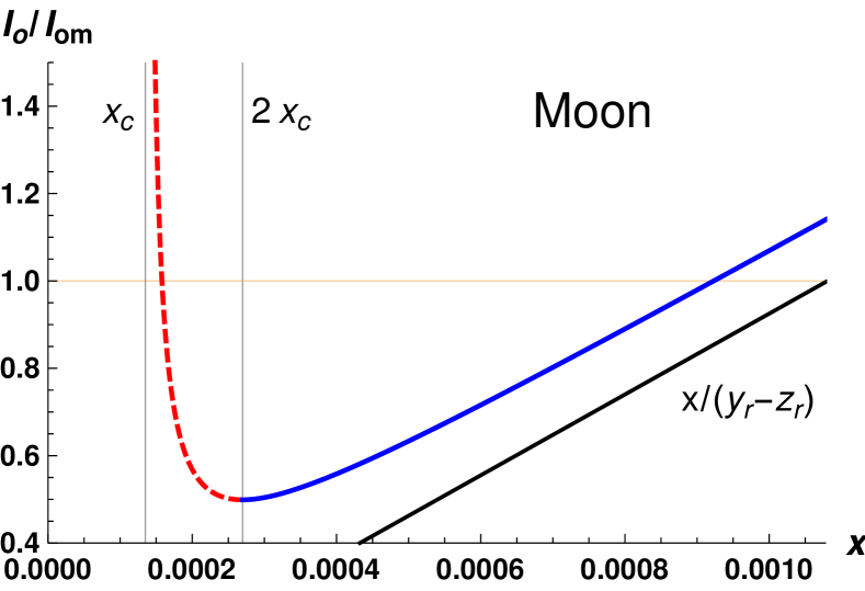
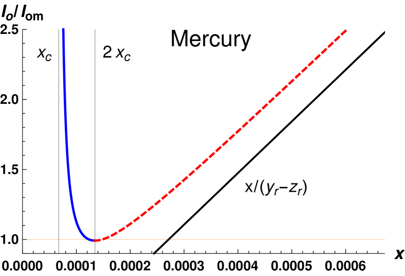
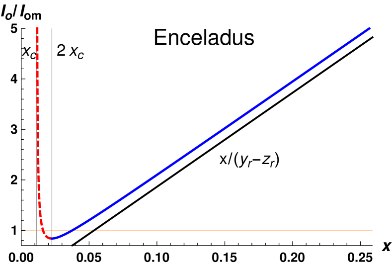
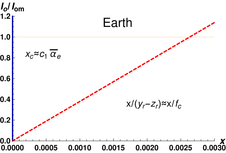
Figure 4: Diagram:Vertical axis $\frac{{\,\rm I}_{\circ}}{{\rm I}_{\circ m}}$ and horizontal axis $x_{\ell ar}$ (solid-blue line) and $x_{dwr}$ (dashed-red line). $x_{dwr}$ (NDFW) and $x_{\ell ar}$ (FLL) are angular frequencies of cycles per sidereal day ($2\pi/\omega$) in the slow frame $\mathrm{K}_{s}$ (see Footnote 16 for the relation to angular frequencies in the inertial frame). The values of $c_{1}$ and $c_{2}$ are from Footnote 11.Other data for the Earth, Mercury, and Moon were taken from Tables 8 and 9 and references cited in their captions. The $k_{2}=0.014$ of Enceladus is from Běhounková et al. (2017), the values $\overline{\alpha}_{e}=0.0162$ and $\overline{\gamma}=0.0183$ were computed using the gravitational coefficients in Iess et al. (2014), and other data are from Thomas et al. (2016). The approximated values of $1+f_{0}=\frac{{\,\rm I}_{\circ}}{{\rm I}_{\circ m}}$ are: $1+7\times 10^{-4}$ (Moon), $4.2$ (Enceladus), $2.35$ (Mercury), $1.13$ (Earth).

We will present explicit formulas in two cases. At first suppose that there is no spin-orbit resonance $c_{2}=0$, the extended body is axisymmetric $\overline{\gamma}=0$, and the gravitational coefficient $c_{1}\ll 1$ (for the Earth $c_{1}=0.000027$). In this case $p_{r}\approx(f_{c}+c_{1}\overline{\alpha}_{e})/2$, $q_{r}\approx(f_{c}-c_{1}\overline{\alpha}_{e})/2$, and the eigenfrequencies are approximately

$$\sigma_{dw}=\omega\left(1+\frac{{\,\rm I}_{\circ}}{{\rm I}_{\circ m}}f_{c}\right)\quad\text{and}\quad\sigma_{\ell a}=\omega\left(1+c_{1}\overline{\alpha}_{e}\right)\,.$$ (6.132)

The formula we obtained for $\sigma_{dw}$ agrees with that for $\sigma_{2}$ in equation (37) in Mathews et al. (2002) . In the case of the Earth the motion associated with $\sigma_{\ell a}$ ($2\pi/(\omega c_{1}\overline{\alpha}_{e})\approx 30834$ years) can be understood as a “precession on precession”: the mantle spin precesses in the inertial frame, this precessing vector defines the $\mathbf{e}_{3}$-axis of the slow frame, and libration in latitude is a secondary precession of the mantle spin with respect to the $\mathbf{e}_{3}$-axis of the slow frame.

The second case we will analyse is that of a body in 1:1 spin orbit resonance and we will take the Moon as an example. In this case both $c_{1}$ and $c_{2}$ are of the order of one (see footnote 11). The moment of inertia of the core of the Moon is small, $f_{0}={\rm I}_{\circ c}/{\rm I}_{\circ m}\approx 7\times 10^{-4}$, such that, up to small corrections, $x_{dw}=y_{r}$, $x_{\ell a}=z_{r}$ and

$$\sigma_{dw}=i\,\omega(1+f_{c})\quad\sigma_{\ell a}=i\,\omega\Big{(}1+c_{1}\overline{\alpha}_{e}+\frac{c_{2}}{2}\overline{\gamma}-C_{r}\left(c_{1}^{2}+c_{2}^{2}\right)\Big{)}\,$$ (6.133)

(for the Moon the term proportional to $C_{r}$ in $\sigma_{\ell a}$ can also be neglected). The expression for $\sigma_{dw}$ in equation (6.133) is the same as the one due to Petrova and Gusev as reported in Williams and Boggs (2008) (p.111) and Rambaux and Williams (2011) (equation (16)).

Using the parameters in Tables 9 and 10 we find from equation (6.133) that in the inertial frame the NDFW has a period equal to 469 years (this period is considerably larger than that reported in Williams and Boggs (2008), which is $197$ years, but is almost within the range of the most recent estimate $367\pm 100$ years Viswanathan et al. (2019)). In the same way, we obtain from equation (6.133) that in the inertial frame the FLL mode has a period of $80.84$ years (the value obtained from observations in Rambaux and Williams (2011) is 80.86 years).

6.4 Eigenmodes and Summary.

In this paragraph we present the rotational eigenmodes in time domain and we summarise the results obtained in this Section.

For each one of the vectors $\boldsymbol{\alpha}_{m}$, $\boldsymbol{\alpha}_{c}$, and $\boldsymbol{\delta}\mathbf{B}$, only the components that are different from zero at leading order in the small quantities will be shown. The components of $\boldsymbol{\delta}\mathbf{B}$ are determined by equation (6.112) and only the components $(1,2),(1,3)$, and $(2,3)$ will appear in the expressions of the eigenmatrix. We will assume that the variations of the moment of inertia due to tides and time-variable centrifugal forces are small enough (hypothesis (4.62)), so that we can use the vector $\boldsymbol{\beta}$ (equation (4.65)) with components

$$\beta_{1}(t)=\frac{B_{T,m23}(t)}{\overline{\alpha}}\,,\ \beta_{2}(t)=-\frac{B_{T,m13}(t)}{\overline{\beta}}\,,\ \beta_{3}(t)=\frac{B_{T,m12}(t)}{\overline{\gamma}}\,$$

to represent the eigenmatrix $\boldsymbol{\delta}\mathbf{B}$. We recall that $\boldsymbol{\beta}$ gives the angular displacement of the principal axes frame from the prestress frame, $(\mathbb{I}+\boldsymbol{\widehat{\beta}}):\mathrm{K}_{p}\to\mathrm{K}_{m}$.

The $(\boldsymbol{\alpha}_{m},\boldsymbol{\alpha}_{c})$ components of the eigenmodes above represent oscillations with respect to the guiding frame. The analysis of these oscillations using other frames follows the ideas in Footnote 15.

The motion of the frame of the principal axes of inertia with respect to the guiding frame is given by $(\mathbb{I}+\boldsymbol{\widehat{\alpha}}_{p}):\mathrm{K}_{p}\to\mathrm{K}_{g}$, where $\boldsymbol{\alpha}_{p}=\boldsymbol{\alpha}_{m}+\boldsymbol{\beta}$.

All the eigenmodes below are composed by two oscillating vectors. Only one of these vectors will be given, because the second one can be obtained by exchanging $\big{(}\cos(\sigma t),\sin(\sigma t)\big{)}\to\big{(}\sin(\sigma t),-\cos(\sigma t)\big{)}$, which corresponds to the time translation $t\to t-\frac{\pi}{2\sigma}$.

The complex compliance $C$ is related to the complex Love number as (equation (6.111)):

$$C(i\sigma)=\frac{\omega^{2}R^{5}}{3{\,\rm I}_{\circ}G}\,k(\sigma)\,.$$

The “characteristic time” $\tau$ is defined as (equation (6.118)):

$$C(\lambda)=C(0)(1-\lambda\tau)+\mathcal{O}(\lambda^{2})\,,\quad\text{where}\quad\tau=-\frac{1}{C(0)}\frac{\partial C}{\partial\lambda}(0)$$

Note that the definition of $\tau$ does not depend on the particular model used for the rheology of the mantle. In terms of the parameters of the rheology, $\tau$ is given in equation: (6.119) Kelvin-Voigt, (6.120) generalized Maxwell, (6.119) generalized Voigt, and (8.172) Andrade.

Free libration in longitude.

$$\begin{split}\lambda_{\ell o}=&i\,\omega\sqrt{\frac{{\,\rm I}_{\circ}}{{\rm I}_{m0}}(\xi_{2}-\xi_{1})\,\,\Big{(}\overline{\gamma}-C(0)\,(\xi_{2}-\xi_{1})\Big{)}}\\ &-\frac{\eta_{c}}{2}\,\frac{{\rm I}_{\circ c}}{{\,\rm I}_{\circ}}-\tau\omega^{2}C(0)\frac{{\,\rm I}_{\circ}}{{\rm I}_{\circ m}}\frac{(\xi_{2}-\xi_{1})^{2}}{2}\\ :=&i\sigma_{\ell o}-\nu_{\ell o}\,.\end{split}$$ (6.134)

Only the coordinates $\alpha_{m3}$, $\alpha_{c3}$, and $\beta_{3}$ of the eigenmodes are nonnull. The eigenvector is:

$$\begin{split}&\begin{bmatrix}\alpha_{m3}\\ \alpha_{c3}\\ \beta_{3}\end{bmatrix}={\rm e}^{-t\nu_{\ell o}}\begin{bmatrix}&\cos(\sigma_{\ell o}t)\\ \frac{\eta_{c}}{\sigma_{\ell o}}\frac{{\rm I}_{\circ m}}{{\,\rm I}_{\circ}}&\sin(\sigma_{\ell o}t)\\ -\frac{C(0)(\xi_{2}-\xi_{1})}{\overline{\gamma}}&\cos(\sigma_{\ell o}t)\end{bmatrix}\\ \end{split}$$ (6.135)

The free libration in longitude eigenmode is represented in Figure 5.

Figure 5: Left:3-D representation of the oscillations of free librations in longitude. Positions at constant time intervals of the frame of the mantle $\mathrm{K}_{m}$ (of the core $\mathrm{K}_{c}$) are depicted by black dots on the external sphere (on the internal sphere) that is fixed in the guiding-frame $\mathrm{K}_{g}$. The white dots indicate the initial condition. Right: Relative positions of the several vectors on the equatorial plane of $\mathrm{K}_{g}$. Note: Deformations decrease the amplitude of librations of $\mathrm{K}_{p}$, the frame of principal axes of the mantle, in comparison to the librations of $\mathrm{K}_{m}$. The angle $\beta_{3}$ between these two frames tends to zero in the limit as the mantle becomes rigid.

Wobble.

$$\begin{split}\lambda_{w}=&i\,\omega\,\frac{{\,\rm I}_{\circ}}{{\rm I}_{\circ m}}\sqrt{\xi_{1}\xi_{2}\Big{(}\overline{\alpha}-\xi_{1}C(0)\Big{)}\Big{(}\overline{\beta}-\xi_{2}C(0)\Big{)}}\\ &\\ &-\frac{\eta_{c}}{2}\frac{{\rm I}_{\circ c}}{{\rm I}_{\circ m}}\Big{(}\overline{\alpha}\xi_{1}+\overline{\beta}\xi_{2}-C(0)(\xi_{1}^{2}+\xi_{2}^{2})\Big{)}\\ &-\tau\omega^{2}C(0)\frac{{\,\rm I}_{\circ}^{2}}{{\rm I}^{2}_{\circ m}}\frac{\xi_{1}\xi_{2}}{2}(\overline{\beta}\xi_{1}+\overline{\alpha}\xi_{2}-2C(0)\xi_{1}\xi_{2})\\ :=&i\sigma_{w}-\nu_{w}\,.\end{split}$$ (6.136)

The coordinates $\alpha_{m3}$, $\alpha_{c3}$, and $\beta_{3}$ of the eigenmodes are null. The eigenvector is:

$$\begin{split}&\begin{bmatrix}\alpha_{m1}\\ \alpha_{m2}\end{bmatrix}={\rm e}^{-t\nu_{w}}\begin{bmatrix}&\cos(\sigma_{w}t)\\ \alpha_{w2}&\sin(\sigma_{w}t)\end{bmatrix}\,,\begin{bmatrix}\beta_{1}\\ \beta_{2}\end{bmatrix}=-{\rm e}^{-t\nu_{w}}C(0)\begin{bmatrix}\frac{\xi_{1}}{\overline{\alpha}}&\cos(\sigma_{w}t)\\ \frac{\xi_{2}}{\overline{\beta}}\alpha_{w2}&\sin(\sigma_{w}t)\end{bmatrix}\\ &\\ &\begin{bmatrix}\alpha_{c1}\\ \alpha_{c2}\end{bmatrix}=f_{c}\begin{bmatrix}\alpha_{m1}(t)\\ \alpha_{m2}(t)\end{bmatrix}+{\rm e}^{-t\nu_{w}}\frac{\eta_{c}}{\omega}\frac{{\rm I}_{\circ m}}{{\,\rm I}_{\circ}}\begin{bmatrix}\alpha_{w2}&\ \ \sin(\sigma_{w}t)\\ &-\cos(\sigma_{w}t)\end{bmatrix}\,,\end{split}$$ (6.137)

where

$$\alpha_{w2}:=\sqrt{\frac{\xi_{1}(\overline{\alpha}-C(0)\xi_{1})}{\xi_{2}(\overline{\beta}-C(0)\xi_{2})}}\,.$$

The wobble eigenmode is represented in Figure 6.

Figure 6: Representation of the oscillations of the wobble. The Figure shows the motion of $\mathrm{K}_{m}$ and $\mathrm{K}_{c}$ with respect to $\mathrm{K}_{g}$ as explained in the caption of Figure 5. The $\mathbf{e}_{3}$-axis of $\mathrm{K}_{m}$ traces an elliptical path. The minor axis of the ellipsis is along the $\mathbf{e}_{1}$-axis of $\mathrm{K}_{g}$ (the principal axis of minimum moment of inertia $\overline{I}_{1}$), which in the case of the Moon is towards the Earth. Using the formulas given in this paper with $\xi_{1}$ and $\xi_{2}$ given in Footnote 11, $C(0)=\omega^{2}/(\mu_{0}+\gamma)$ with $\mu_{0}$ and $\gamma$ given in Table 9, $\overline{\alpha}$ and $\overline{\beta}$ obtained from the data in Table 10 (Moon) and from Mazarico et al. (2014) (Mercury, $\overline{\alpha}=0.000099$, $\overline{\beta}=0.000192$), we obtain (minor axis)/(major axis)=$\sqrt{\frac{\xi_{1}(\overline{\alpha}-C(0)\xi_{1})}{\xi_{2}(\overline{\beta}-C(0)\xi_{2})}}$= 0.402 (Moon) and 0.553 (Mercury). The value for the Moon reported in Williams and Boggs (2008) is 0.406.

Nearly Diurnal Free Wobble (NDFW) and Free Libration in Latitude (FLL).

$$\begin{split}\lambda_{dw}&=i\omega(1+x_{dw})=i\sigma_{dw}-\nu_{dw}\\ \lambda_{\ell a}&=i\omega(1+x_{\ell a})=i\sigma_{\ell a}-\nu_{\ell a}\,,\end{split}$$ (6.138)

where $x_{dw}$ and $x_{\ell a}$ are the solutions to the equation

$$\begin{split}&x^{2}-x(f_{0}+1)(y+z)+(f_{0}+1)z\,y=0\,,\\ &\text{and}\\ &z=c_{1}\overline{\alpha}_{e}+\frac{c_{2}}{2}\overline{\gamma}-C(i\omega)\left(c_{1}^{2}+c_{2}^{2}\right)\ \Big{(}\text{FLL eigenvalue for}\ {\rm I}_{\circ c}=0\Big{)}\,,\\ &y=f_{c}+i\frac{\eta_{c}}{\omega}\frac{{\rm I}_{\circ m}}{{\,\rm I}_{\circ}}\quad\qquad\qquad\qquad\ \ \,\Big{(}\text{NDFW eigenvalue for}\ {\rm I}_{\circ c}=0\Big{)}\,.\end{split}$$ (6.139)

The FLL and NDFW eigenvalues have the same nature and are not easily distinguishable, see equations (C.215) and (C.216).

The coordinates $\alpha_{m3}$, $\alpha_{c3}$, and $\beta_{3}$ of the eigenmodes are null. We will choose a normalisation of the eigenvectors such that for both modes NDFW and FLL the components of $\boldsymbol{\alpha}_{m}$ and $\boldsymbol{\beta}$ are the same and given by:

$$\begin{bmatrix}\alpha_{m1}\\ \alpha_{m2}\end{bmatrix}={\rm e}^{-t\nu}\begin{bmatrix}\ \ \cos(\sigma t)\\ -\sin(\sigma t)\end{bmatrix}\,,\begin{bmatrix}\beta_{1}\\ \beta_{2}\end{bmatrix}={\rm e}^{-t\nu}\begin{bmatrix}\frac{\xi_{1}-1}{\overline{\alpha}}&\big{(}C_{i}\sin(\sigma t)-C_{r}\cos(\sigma t)\big{)}\\ \frac{\xi_{2}-1}{\overline{\beta}}&\big{(}C_{r}\sin(\sigma t)+C_{i}\cos(\sigma t)\big{)}\,,\end{bmatrix}$$ (6.140)

where: $(\nu,\sigma)=(\nu_{dw},\sigma_{dw})$ for the NDFW, $(\nu,\sigma)=(\nu_{\ell a},\sigma_{\ell a})$ for the FLL, and $C(i\omega)=C_{r}+iC_{i}$.

For the NDFW

$$\boldsymbol{\alpha}_{c}={\rm Re}\left\{\exp\big{(}i\,\sigma_{dw}t-\nu_{dw}t\big{)}\frac{1}{f_{0}}\left(-1+\frac{x_{\ell a}}{y}\right)\begin{bmatrix}1\\ i\\ 0\end{bmatrix}\right\}$$ (6.141)

and for the FLL

$$\boldsymbol{\alpha}_{c}={\rm Re}\left\{\exp\big{(}i\,\sigma_{\ell a}t-\nu_{\ell a}t\big{)}\frac{1}{f_{0}}\left(-1+\frac{x_{dw}}{y}\right)\begin{bmatrix}1\\ i\\ 0\end{bmatrix}\right\}$$ (6.142)

where: $y=f_{c}+i\frac{\eta_{c}}{\omega}\frac{{\rm I}_{\circ m}}{{\,\rm I}_{\circ}}$, $x_{\ell a}=x_{\ell ar}+i\,\nu_{\ell a}/\omega$, and $x_{dw}=x_{dwr}+i\,\nu_{dw}/\omega$.

The NDFW and FLL eigenmodes are represented in Figure 7.

Figure 7: Representation of the oscillations of the NDFW (LEFT) and FLL (RIGHT). The Figures show the motion of $\mathrm{K}_{m}$ and $\mathrm{K}_{c}$ with respect to $\mathrm{K}_{g}$ as explained in the caption of Figure 5. The only difference between the NDFW and the FLL is the relative amplitude of the oscillations of the mantle and the core. For the Moon the amplitude of librations of the core is larger for the NDFW and the opposite is true for the FLL. Using the parameters given in Table 10 (Moon) we obtain (amplitude core)/(amplitude mantle)= 7107 (NDFW) and 0.2010 (FLL).

7 The offset of the rotation axes of mantle and core from the Cassini state of the rigid-body approximation.

The definition of guiding motion is based on the hypothesis that the extended body rotates almost steadily as a rigid body. It is therefore natural to assume in the theoretical determination of a guiding motion that the extended body is rigid. The slow frame determined from the rigid-body motion is in general non inertial due to axial precession. In this Section we investigate the effect of inertial forces in the slow frame when we replace a rigid body in guiding motion for a body made of a rigid mantle and a fluid core.

The theoretical determination of the Cassini state of a rigid body in s-to-2 spin-orbit resonance (e.g. Moon) Peale (1969) is done by means of equations in which the torque is averaged after being written in the orbital frame $\mathrm{K}_{or}$, which is a frame that precesses with the orbit of the point mass and is given by $\mathbf{R}_{or}=\mathbf{R_{3}}(\Omega_{p})\mathbf{R_{1}}(\iota_{p}):\mathrm{K}_{or}\to\kappa$ . In the following we consider the case of an extended body in s-to-2 spin-orbit resonance with a point mass. The case of no spin-orbit resonance is easier and will be treated in Section 7.1.

In Appendix A (equations (A.184), (A.185), and (A.186)) we parameterized the guiding motion associated to a Cassini state as $\mathbf{R_{g}}=\mathbf{R_{3}}(\psi_{g})\mathbf{R_{1}}(\theta_{g})\mathbf{R_{3}}(\phi_{g})$, where: $\theta_{g}$ ($\dot{\theta}_{g}=0$) is the inclination of the body equator to the $(\mathbf{e}_{1},\mathbf{e}_{2})$-plane in $\kappa$ (the Laplace plane or invariable plane), $\psi_{g}$ ($\ddot{\psi}_{g}=0$) is the longitude of the ascending node of the body equator, and $\phi_{g}$ ($\ddot{\phi}_{g}=0$) is the angle between the ascending node and Axis 1 (a principal axis of smallest moment of inertia). The slow frame $\mathbf{R}_{s}:\mathrm{K}_{s}\to\kappa$ is defined by $\mathbf{R}_{s}=\mathbf{R}_{g}\mathbf{R_{3}}^{-1}(\omega\,t)=\mathbf{R_{3}}(\psi_{g})\mathbf{R_{1}}(\theta_{g})\mathbf{R_{3}}(\zeta)$ where $\zeta=\phi_{g}-\omega t$ and (due to equation (2.15)) $\dot{\zeta}=-\dot{\psi}_{g}\cos\theta_{g}$. These definitions imply (see equation (B.208))

$$\boldsymbol{\omega}_{s,g}=\dot{\psi}_{g}\sin\theta_{g}\left(\begin{array}[]{c}\sin\phi_{g}\\ \cos\phi_{g}\\ 0\end{array}\right)\,,\quad\dot{\boldsymbol{\omega}}_{s,g}=\dot{\phi}_{g}\dot{\psi}_{g}\sin\theta_{g}\left(\begin{array}[]{c}\ \ \,\cos\phi_{g}\\ -\sin\phi_{g}\\ 0\end{array}\right)\,.$$ (7.143)

The guiding motion becomes simpler in the “precessional frame” $\mathrm{K}_{pr}$ defined as:

$$\mathbf{R}_{3}(\psi_{g})\mathbf{R}_{1}(\theta_{g}):\mathrm{K}_{pr}\to\kappa\Longrightarrow\left\{\begin{array}[]{ll}\mathbf{R}_{3}(\phi_{g})&:\mathrm{K}_{g}\to\mathrm{K}_{pr}\\ \mathbf{R}_{3}(\zeta)&:\mathrm{K}_{s}\to\mathrm{K}_{pr}\,.\end{array}\right.$$ (7.144)

Note that $\mathrm{K}_{s}$ ($\mathrm{K}_{g}$) rotates slowly (fastly) with angular velocity $\dot{\zeta}=-\dot{\psi}_{g}\cos\theta_{g}$ ($\dot{\phi}_{g}$) inside $\mathrm{K}_{pr}$, in such a way that the $\mathbf{e}_{3}$-axis of $\mathrm{K}_{s}$ ($\mathrm{K}_{g}$) remains aligned with the $\mathbf{e}_{3}$-axis of $\mathrm{K}_{pr}$. The angular velocity of the precessional frame $\boldsymbol{\omega}_{pr}=\dot{\psi}_{g}\mathbf{e}_{3}\in\kappa$ is represented by a constant vector $\boldsymbol{\omega}_{pr,pr}=\dot{\psi}_{g}\sin\theta_{g}\mathbf{e}_{2}+\dot{\psi}_{g}\cos\theta_{g}\mathbf{e}_{3}$ in $\mathrm{K}_{pr}$, and the angular velocity of the guiding frame, which is given by

$$\boldsymbol{\omega}_{g,pr}=\mathbf{R}_{3}(\phi_{g})\boldsymbol{\omega}_{g,g}=\omega\mathbf{e}_{3}+\mathbf{R}_{3}(\phi_{g})\boldsymbol{\omega}_{s,g}=\omega\mathbf{e}_{3}+\dot{\psi}_{g}\sin\theta_{g}\mathbf{e}_{2}\,,$$ (7.145)

is also constant in $\mathrm{K}_{pr}$.

By definition, the guiding motion is a solution to Euler’s equation after time-averaging in $\mathrm{K}_{pr}$. If we use: the notation $\langle f\rangle=\lim_{T\to\infty}\frac{1}{T}\int_{0}^{T}f(t)dt$, that $\dot{\phi}_{g}$ is constant, $[\overline{\mathbf{I}},\overline{\mathbf{J}}]=0$, and $\mathbf{R}_{3}(\phi_{g}):\mathrm{K}_{g}\to\mathrm{K}_{pr}$, then we obtain

$$\begin{split}&\langle\mathbf{I}_{pr}\rangle=\frac{1}{2\pi}\int_{0}^{2\pi}\mathbf{R}_{3}^{-1}(\phi_{g})\overline{\mathbf{I}}\mathbf{R}_{3}(\phi_{g})d\phi_{g}=\left(\begin{array}[]{ccc}\frac{\overline{I}_{1}+\overline{I}_{2}}{2}&0&0\\ 0&\frac{\overline{I}_{1}+\overline{I}_{2}}{2}&0\\ 0&0&\overline{I}_{3}\end{array}\right)\ \ \text{and}\\ &\Big{\langle}\frac{d}{dt}\mathbf{I}_{pr}\boldsymbol{\omega}_{g,pr}+\boldsymbol{\omega}_{pr,pr}\times\mathbf{I}_{pr}\boldsymbol{\omega}_{g,pr}\Big{\rangle}=\boldsymbol{\omega}_{pr,pr}\times\langle\mathbf{I}_{pr}\rangle\boldsymbol{\omega}_{g,pr}=\\ &=\left(\begin{array}[]{c}\overline{I}_{3}\dot{\phi}_{g}\dot{\psi}_{g}\sin\theta_{g}+\mathcal{O}(\dot{\psi}_{g}^{2})\\ 0\\ 0\end{array}\right)=\Big{\langle}\mathbf{R}_{3}^{-1}(\phi_{g})[\overline{\mathbf{I}},\overline{\mathbf{J}}+\boldsymbol{\delta}\mathbf{J}(t)]\mathbf{R}_{3}(\phi_{g})\Big{\rangle}^{\vee}=\\ &=\left(\begin{array}[]{c}(\overline{I}_{3}-\overline{I}_{2})\big{\langle}\delta J_{23}(t)\cos(t\dot{\phi}_{g})\big{\rangle}+(\overline{I}_{3}-\overline{I}_{1})\big{\langle}\delta J_{13}(t)\sin(t\dot{\phi}_{g})\big{\rangle}\\ (\overline{I}_{1}-\overline{I}_{3})\big{\langle}\delta J_{13}(t)\cos(t\dot{\phi}_{g})\big{\rangle}+(\overline{I}_{3}-\overline{I}_{2})\big{\langle}\delta J_{23}(t)\sin(t\dot{\phi}_{g})\big{\rangle}\\ (\overline{I}_{2}-\overline{I}_{1})\big{\langle}\delta J_{12}(t)\big{\rangle}\end{array}\right)\,.\end{split}$$ (7.146)

By definition, the average value of $\delta J_{12}$ is zero. The average $\big{\langle}\delta J_{23}(t)\sin(t\dot{\phi}_{g})\big{\rangle}$ is one half of the Fourier coefficient associated with $\sin\phi_{g}$ of the Fourier expansion of $\delta J_{23}$. The computation of this Fourier coefficient, and of the others, is similar to the computation of the constants $c_{1}$ and $c_{2}$ done in the Appendix A. The result is:

$$\begin{split}\big{\langle}\delta J_{23}(t)\cos(t\dot{\phi}_{g})\big{\rangle}&=\left(\frac{3Gm_{p}}{2a_{p}^{3}}\right)\frac{1}{4}\Big{(}X^{-3,2}_{s}(e)+\big{(}X^{-3,2}_{s}(e)-2X^{-3,0}_{0}(e)\big{)}\cos\chi_{p}\Big{)}\sin\chi_{p}\\ \big{\langle}\delta J_{13}(t)\sin(t\dot{\phi}_{g})\big{\rangle}&=-\left(\frac{3Gm_{p}}{2a_{p}^{3}}\right)\frac{1}{4}\Big{(}X^{-3,2}_{s}(e)+\big{(}X^{-3,2}_{s}(e)+2X^{-3,0}_{0}(e)\big{)}\cos\chi_{p}\Big{)}\sin\chi_{p}\\ \big{\langle}\delta J_{23}(t)\sin(t\dot{\phi}_{g})\big{\rangle}&=\big{\langle}\delta J_{13}(t)\cos(t\dot{\phi}_{g})\big{\rangle}=0\,,\end{split}$$ (7.147)

where $X^{-3,0}_{0}(e)$ and $X^{-3,2}_{s}(e)$ are the Hansen coefficients given in Appendix A and $\chi_{p}$ is the obliquity, namely the angle between the body axis of largest moment of inertia ($\mathbf{e}_{3}\in\mathrm{K}_{g}$) and the normal to the orbital plane. We remark that $\mathbf{e}_{3}\in\mathrm{K}_{g}$ is the spin axis of the guiding motion with respect to the orbital frame ($\mathbf{R}_{or}^{-1}\mathbf{R}_{g}:\mathrm{K}_{g}\to\mathbf{\mathrm{K}}_{or}$). According to Footnote 18, $\chi_{p}=\theta_{g}-\iota_{p}$ for Cassini state 1 (e.g. Mercury), or $\chi_{p}=\theta_{g}+\iota_{p}$ for Cassini state 2 (e.g. Moon).

Equations (7.146) and (7.147) imply that the Cassini state is equal to the guiding motion $\mathbf{R_{g}}=\mathbf{R_{3}}(\psi_{g})\mathbf{R_{1}}(\theta_{g})\mathbf{R_{3}}(\phi_{g})$ if

$$\dot{\psi}_{g}\dot{\phi}_{g}\sin\theta_{g}=-\frac{3}{2}\frac{Gm_{p}}{a_{p}^{3}}\sin\chi_{p}\left(\overline{\alpha}_{e}X^{-3,0}_{0}\cos\chi_{p}+\frac{\overline{\gamma}}{4}X^{-3,2}_{s}(1+\cos\chi_{p})\right):=\cal P\,,$$ (7.148)

where $\overline{\alpha}_{e}=\frac{\overline{I}_{3}-(\overline{I}_{1}+\overline{I}_{2})/2}{\overline{I}_{3}}$ and $\overline{\gamma}=\frac{\overline{I}_{2}-\overline{I}_{1}}{\overline{I}_{3}}$. Equation (7.148) is that obtained by Peale (1969), as presented in Boué (2020). The signs of the angles in equation (7.148) have been a source of mistakes (Baland et al. (2017) Section 6.1.1). Our sign conventions are: $\dot{\psi}_{g}<0$, $\dot{\phi}_{g}=\omega-\dot{\psi}_{g}\cos\theta_{g}>0$, $\theta_{g}>0$ , $\chi_{p}>0$ , and $\iota_{p}>0$. There are two possible relations among $\theta_{g}$, $\chi_{p}$, and $\iota_{p}$: $\theta_{g}=\chi_{p}+\iota_{p}$ for the Cassini state 1 (e.g. Mercury) and $\theta_{g}=\chi_{p}-\iota_{p}$ for Cassini state 2 (e.g. Moon). For a given $\iota_{p}$, the solutions $\chi_{p}$ to equation (7.148) in case 1 are the same as those in case 2 after a change of sign. The Cassini state we are interested in is obtained in the following way. Given $\iota_{p}$ choose $\theta_{g}=\chi_{p}+\iota_{p}$ and solve for $\chi_{p}$. Among the solutions with $-\pi<\chi_{p}\leq\pi$ choose the one, denoted as $\tilde{\chi}_{p}$, with the smallest absolute value. If $\tilde{\chi}_{p}>0$ ($\tilde{\chi}_{p}<0$), then $\chi_{p}=\tilde{\chi}_{p}$ ($\chi_{p}=-\tilde{\chi}_{p}$) and we have a Cassini state 1 with $\theta_{g}=\chi_{p}+\iota_{p}$ (a Cassini state 2 with $\theta_{g}=\chi_{p}-\iota_{p}$).

In the follwowing we restrict the tidal force matrix $\boldsymbol{\delta}\mathbf{J}_{g}$ to its Fourier modes in $\cos\phi_{g}$ and $\sin\phi_{g}$, and write $\delta J_{g12}(t)=0$,

$$\begin{split}\delta J_{g13}(t)&=2\big{\langle}\delta J_{13}(t)\sin(t\dot{\phi}_{g})\big{\rangle}\sin(\phi_{g})=\frac{\overline{I}_{3}}{\overline{I}_{3}-\overline{I}_{1}}({\cal P-R})\sin(\phi_{g})\\ \delta J_{g23}(t)&=2\big{\langle}\delta J_{23}(t)\cos(t\dot{\phi}_{g})\big{\rangle}\cos\phi_{g}=\frac{\overline{I}_{3}}{\overline{I}_{3}-\overline{I}_{2}}({\cal P+R})\cos\phi_{g}\,,\end{split}$$ (7.149)

where we have used equations (7.147) and (7.148) and the definition

$${\cal R}:=\frac{3}{2}\frac{Gm_{p}}{a_{p}^{3}}\sin\chi_{p}\left(\frac{\overline{\alpha}_{e}}{2}X^{-3,2}_{s}(1+\cos\chi_{p})+\frac{\overline{\gamma}}{2}X^{-3,0}_{0}\cos\chi_{p}\right)\,.$$ (7.150)

The guiding motion solves the forced rigid-body equations only in an average sense. The residue we obtain after the substitution of the guiding motion into the rigid-body equation written in the guiding frame is, after using equations (2.15), (7.143), and (7.149), and ${\cal P}=\dot{\psi}_{g}\dot{\phi}_{g}\sin\theta_{g}$ (Peale’s equation):

$$\begin{split}&[\overline{\mathbf{I}},\boldsymbol{\delta}\mathbf{J}_{g}]^{\vee}-\overline{\mathbf{I}}\dot{\boldsymbol{\omega}}_{g,g}-\dot{\boldsymbol{\omega}}_{g,g}\times\overline{\mathbf{I}}\dot{\boldsymbol{\omega}}_{g,g}=\left(\begin{array}[]{c}\big{(}\overline{I}_{3}-\overline{I}_{2}\big{)}\delta J_{g23}-\overline{I}_{1}\dot{{\omega}}_{s,g1}-\omega\big{(}\overline{I}_{3}-\overline{I}_{2}\big{)}{\omega}_{s,g2}\\ \big{(}\overline{I}_{1}-\overline{I}_{3}\big{)}\delta J_{g13}-\overline{I}_{2}\dot{{\omega}}_{s,g2}-\omega\big{(}\overline{I}_{3}-\overline{I}_{1}\big{)}{\omega}_{s,g1}\\ 0\end{array}\right)=\\ &\left(\begin{array}[]{c}\overline{I}_{3}({\cal P+R})\cos\phi_{g}-(\overline{I}_{1}-\overline{I}_{2}+\overline{I}_{3})\dot{\phi}_{g}\dot{\psi}_{g}\sin\theta_{g}\cos\phi_{g}\\ \overline{I}_{3}({\cal R-P})\sin\phi_{g}-(\overline{I}_{1}-\overline{I}_{2}-\overline{I}_{3})\dot{\phi}_{g}\dot{\psi}_{g}\sin\theta_{g}\sin\phi_{g}\\ 0\end{array}\right)=\left(\begin{array}[]{c}\big{(}(\overline{I}_{2}-\overline{I}_{1}){\cal P}+\overline{I}_{3}{\cal R}\big{)}\cos\phi_{g}\\ \left((\overline{I}_{2}-\overline{I}_{1}){\cal P}+\overline{I}_{3}{\cal R}\right)\sin\phi_{g}\\ 0\end{array}\right)\,\end{split}$$ (7.151)

where terms of order $\dot{\psi}_{g}^{2}$ were neglected.

Now, we will investigate the motion in the guiding frame of a body with a deformable mantle and a fluid core. The analysis will be restricted to the frequency $\dot{\phi}_{g}$.

The mean moment of inertia of the whole body can be decomposed as $\overline{\mathbf{I}}=\overline{\mathbf{I}}_{m}+\overline{\mathbf{I}}_{c}$. If we write $\overline{\mathbf{I}}\dot{\boldsymbol{\omega}}_{s,g}=(\overline{\mathbf{I}}_{m}+\overline{\mathbf{I}}_{c})\dot{\boldsymbol{\omega}}_{s,g}$ and use equation (7.151) and $\mathbf{I}_{c}\dot{\boldsymbol{\omega}}_{s,g}=\dot{\phi}_{g}\dot{\psi}_{g}\sin\theta_{g}\mathbf{I}_{c}\mathbf{R}^{-1}_{3}(\phi_{g})\mathbf{e}_{1}={\cal P}\mathbf{I}_{c}\mathbf{R}^{-1}_{3}(\phi_{g})\mathbf{e}_{1}$, then we can write the right hand side of equation (5.92) (the torque) as

$$\begin{split}&\big{(}\overline{I}_{3}-\overline{I}_{2}\big{)}\langle\delta J\rangle_{g23}-\overbrace{\overline{I}_{m1}}^{\overline{I}_{1}-\overline{I}_{c1}}\dot{{\omega}}_{s,g1}-\omega\big{(}\overline{I}_{3}-\overline{I}_{2}\big{)}{\omega}_{s,g2}=\Big{(}(\overline{I}_{2}-\overline{I}_{1}){\cal P}+\overline{I}_{3}{\cal R}+{\cal P}\overline{I}_{c1}\Big{)}\cos\phi_{g}\\ &\big{(}\overline{I}_{1}-\overline{I}_{3}\big{)}\langle\delta J\rangle_{g13}-\underbrace{\overline{I}_{m2}}_{\overline{I}_{2}-\overline{I}_{c2}}\dot{{\omega}}_{s,g2}+\omega\big{(}\overline{I}_{3}-\overline{I}_{1}\big{)}{\omega}_{s,g1}=\Big{(}(\overline{I}_{2}-\overline{I}_{1}){\cal P}+\overline{I}_{3}{\cal R}-{\cal P}\overline{I}_{c2}\Big{)}\sin\phi_{g}\,.\end{split}$$ (7.152)

The torque has a term of forced librations $\big{(}(\overline{I}_{2}-\overline{I}_{1}){\cal P}+\overline{I}_{3}{\cal R}\big{)}\mathbf{R}^{-1}_{3}(\phi_{g})\mathbf{e}_{1}$ that is responsible for the oscillations of the rigid body (and of the mantle) about the Cassini state, and a term $\mathbf{I}_{c}\dot{\boldsymbol{\omega}}_{s,g}$. This last term, which is due to the non-inertial character of the slow frame, will be called the inertial torque. It is partially responsible for the displacement of the spin axis of the mantle from the rigid-body state of Cassini.

The inertial torque that acts upon the mantle is exactly the opposite of that in the right-hand side of equation (5.91), i.e.

$$-\overline{\mathbf{I}}_{c}\dot{\boldsymbol{\omega}}_{s,g}=-{\cal P}\mathbf{I}_{c}\mathbf{R}^{-1}_{3}(\phi_{g})\mathbf{e}_{1}\,,$$ (7.153)

that acts upon the core. Moreover, $-\overline{\mathbf{I}}_{c}\dot{\boldsymbol{\omega}}_{s,g}$ is the unique direct torque upon the core (it does not depend on the relative position of the mantle) regardless all possible tidal-forcing torques that act upon the mantle, and this feature distinguishes the inertial torque $\overline{\mathbf{I}}_{c}\dot{\boldsymbol{\omega}}_{s,g}$ from other torque terms.

The two nonhomogeneous terms in equation (5.104) show that the deformation variables $\boldsymbol{\delta}\mathbf{B}$ are under the effect of both tidal and inertial torques. Equations (7.149) and (7.153) can be used to write the two non-homogeneous terms in equation (5.104) as

$$\begin{split}&-\omega\omega_{s,g1}+\delta J_{g13}=\frac{(\overline{I}_{1}{\cal P}-\overline{I}_{3}{\cal R})}{\overline{I}_{3}-\overline{I}_{1}}\sin\phi_{g}\\ &\qquad=\frac{3Gm_{p}}{2a_{p}^{3}}\left(-X^{-3,0}_{0}\cos\chi_{p}-X^{-3,2}_{s}\cos^{2}(\chi_{p}/2)\right)\sin\chi_{p}\sin\phi_{g}\\ &-\omega\omega_{s,g2}+\delta J_{g23}=\frac{(\overline{I}_{2}{\cal P}+\overline{I}_{3}{\cal R})}{\overline{I}_{3}-\overline{I}_{2}}\cos\phi_{g}\\ &\qquad=\frac{3Gm_{p}}{2a_{p}^{3}}\left(-X^{-3,0}_{0}\cos\chi_{p}+X^{-3,2}_{s}\cos^{2}(\chi_{p}/2)\right)\sin\chi_{p}\cos\phi_{g}\end{split}$$ (7.154)

where terms of order $\dot{\psi}_{g}^{2}$ were neglected.

Equations: (5.92) for $\boldsymbol{\alpha}_{m}$, (5.91) for $\boldsymbol{\alpha}_{c}$ , and one of the equations (5.105), (5.106), or (5.107) for the deformation variables $\boldsymbol{\delta}\mathbf{B}$, with the forcing terms given respectively by equations (7.152), (7.153), and (7.154) can be easily solved numerically in any particular problem. Nevertheless, in order to understand the motion at frequency $\dot{\phi}_{g}$ in the guiding frame and its consequences in the precessional frame it is interesting to further treat the problem in general form.

To simplify the following analysis we will assume that the principle axes of the core cavity are aligned to those of the mantle, so that both $\mathbf{I}_{m}$ and $\mathbf{I}_{c}$ are diagonal in the frame of the mantle. In this case the equations for $\alpha_{m1},\alpha_{m2},\alpha_{c1},\alpha_{c2}$ decouple from those for $\alpha_{m3},\alpha_{c3}$ and due to $\delta J_{12}=0$ and $\omega_{s,g3}=0$ we can make $\alpha_{m3}=\alpha_{m3}=\delta B_{T,m12}=\delta B_{T,m33}=0$. The solution for the angular variables of the mantle and core can be written as

$$\boldsymbol{\alpha}_{m}=\underbrace{\left(\begin{array}[]{ccc}x_{11}&x_{12}&0\\ x_{21}&x_{22}&0\\ 0&0&1\end{array}\right)}_{:=\mathbf{X}}\left(\begin{array}[]{c}-\cos\phi_{g}\\ \,\ \ \sin\phi_{g}\\ 0\end{array}\right)=-\mathbf{X}\mathbf{R}_{3}^{-1}(\phi_{g})\mathbf{e}_{1}\ \ \text{and}\ \ \boldsymbol{\alpha}_{c}=-\mathbf{Y}\mathbf{R}_{3}^{-1}(\phi_{g})\mathbf{e}_{1}\,,$$ (7.155)

where $\mathbf{X}$ and $\mathbf{Y}$ are matrices with constant coefficients. The solution for the deformation variables can be written in a similar way.

The relations in equation (5.85) imply that $\boldsymbol{\omega}_{m,g}=\boldsymbol{\omega}_{g,g}+\dot{\boldsymbol{\alpha}}_{m}\in\mathrm{K}_{g}$, and so $\boldsymbol{\omega}_{m,pr}=\boldsymbol{\omega}_{g,pr}+\mathbf{R}_{3}(\phi_{g})\dot{\boldsymbol{\alpha}}_{m}$. Using equation (7.155) we obtain

$$\dot{\boldsymbol{\alpha}}_{m}=-\dot{\phi}_{g}\mathbf{X}\dot{\mathbf{R}}_{3}^{-1}(\phi_{g})\mathbf{e}_{1}=-\dot{\phi}_{g}\mathbf{X}\mathbf{R}_{3}^{-1}(\phi_{g})\underbrace{\mathbf{R}_{3}(\phi_{g})\dot{\mathbf{R}}_{3}^{-1}(\phi_{g})}_{-\mathbf{\widehat{e}}_{3}}\mathbf{e}_{1}=\dot{\phi}_{g}\mathbf{X}\mathbf{R}_{3}^{-1}(\phi_{g})\mathbf{e}_{2}$$

and using equation (7.145) and the same reasoning for the core angular velocity we obtain, up to small errors,

$$\begin{split}\boldsymbol{\omega}_{m,pr}&=\omega\mathbf{e}_{3}+\dot{\psi}_{g}\sin\theta_{g}\mathbf{e}_{2}+\dot{\phi}_{g}\mathbf{R}_{3}(\phi_{g})\mathbf{X}\mathbf{R}_{3}^{-1}(\phi_{g})\mathbf{e}_{2}\\ \boldsymbol{\omega}_{c,pr}&=\underbrace{\omega\mathbf{e}_{3}+\dot{\psi}_{g}\sin\theta_{g}\mathbf{e}_{2}}_{\boldsymbol{\omega}_{g,pr}}+\dot{\phi}_{g}\mathbf{R}_{3}(\phi_{g})\mathbf{Y}\mathbf{R}_{3}^{-1}(\phi_{g})\mathbf{e}_{2}\,.\end{split}$$ (7.156)

Note that $\boldsymbol{\omega}_{m,pr}$ and $\boldsymbol{\omega}_{c,pr}$ are not stationary in $\mathrm{K}_{pr}$ unless $\mathbf{X}$ and $\mathbf{Y}$ commute with $\mathbf{R}_{3}(\phi_{g})$. However, the images of $\phi_{g}\to\mathbf{R}_{3}(\phi_{g})\mathbf{X}\mathbf{R}_{3}^{-1}(\phi_{g})\mathbf{e}_{2}$ and $\mathbf{R}_{3}(\phi_{g})\mathbf{Y}\mathbf{R}_{3}^{-1}(\phi_{g})\mathbf{e}_{2}$ are circles in the $(\mathbf{e}_{1},\mathbf{e}_{2})$ plane of $\mathrm{K}_{pr}$ that are centred, respectively, at the points

$$\mathbf{x}:=\begin{bmatrix}\frac{x_{12}-x_{21}}{2}\\ \frac{x_{11}+x_{22}}{2}\\ 0\end{bmatrix}\quad\text{and}\quad\mathbf{y}:=\begin{bmatrix}\frac{y_{12}-y_{21}}{2}\\ \frac{y_{11}+y_{22}}{2}\\ 0\end{bmatrix}\,.$$ (7.157)

The expression for the angular velocity of the mantle can be written as (see Figure 8):

$$\begin{split}&\boldsymbol{\omega}_{m,pr}=\omega\mathbf{e}_{3}+\dot{\psi}_{g}\sin\theta_{g}\mathbf{e}_{2}+\dot{\phi}_{g}\mathbf{x}+\dot{\phi}_{g}A\begin{bmatrix}\cos(2\phi_{g}+h)\\ \sin(2\phi_{g}+h)\end{bmatrix}\\ &A=\frac{1}{2}\sqrt{(x_{12}+x_{21})^{2}+(x_{11}-x_{22})^{2}}\,,\quad\tan h=\frac{x_{22}-x_{11}}{x_{12}+x_{21}}\,.\end{split}$$ (7.158)

Similar expressions hold for $\boldsymbol{\omega}_{c,pr}$.

The offsets of the normalised-angular velocity of the mantle and of the core from the angular velocity of the Cassini state of the rigid-body are given by the nondimensional vectors

$$\begin{split}\boldsymbol{\delta}_{m}&:=\frac{\langle\boldsymbol{\omega}_{m,pr}\rangle-\boldsymbol{\omega}_{g,pr}}{\dot{\phi}_{g}}=\mathbf{x}\in\mathrm{K}_{pr}\quad\text{Mantle offset}\\ \boldsymbol{\delta}_{c}&:=\frac{\langle\boldsymbol{\omega}_{c,pr}\rangle-\boldsymbol{\omega}_{g,pr}}{\dot{\phi}_{g}}=\mathbf{y}\in\mathrm{K}_{pr}\quad\,\text{ Core offset}\,,\end{split}$$ (7.159)

where the brackets indicate that we are neglecting the oscillatory parts of $\boldsymbol{\omega}_{m,pr}$ and $\boldsymbol{\omega}_{c,pr}$. We recall that terms of the order $(\dot{\psi}_{g}/\omega)^{2}$ were neglected during the computations. The angles $\delta_{m}$ have the geometric interpretation given in Figure 8.

Figure 8: LEFT: We denote by $\Sigma\in\kappa$ the shaded plane that contains $\mathbf{e}_{3}$ (the normal to the invariable plane) and $\boldsymbol{\omega}_{g}$ (the angular velocity of the rigid-body approximation). The circles indicate that the precession of $\boldsymbol{\omega}_{g}$ is retrograde, $\dot{\psi}_{g}<0$. The inertial torque rotates $\boldsymbol{\omega}_{g}$ of a small angle $\delta_{m2}$ inside $\Sigma$ and rotates $\boldsymbol{\omega}_{g}$ of a small angle $\delta_{m1}$ perpendicular to $\Sigma$. If $\delta_{m2}>0$ ($\delta_{m2}<0$), then the displacement is towards (opposite to) $\mathbf{e}_{3}$. If $\delta_{m1}<0$ ($\delta_{m1}>0)$, then the displacement is towards (opposite to) the direction of the retrograde axial precession. The angle $|\delta_{m1}|>0$ is entirely due to dissipative effects. RIGHT: The projection of $\boldsymbol{\omega}_{g,pr}/\|\boldsymbol{\omega}_{g,pr}\|$ onto the $(\mathbf{e}_{1},\mathbf{e}_{2})$-plane of the precessional frame $\mathrm{K}_{pr}$. This plane moves in the inertial space always orthogonal to the axis of largest moment of inertia of the rigid-body approximation, with $\mathbf{e}_{1}\in\mathrm{K}_{pr}$ in the direction of the ascending node of the equator of the rigid-body approximation, and $\mathbf{e}_{2}\in\mathrm{K}_{pr}$ pointing towards the pole of the invariable plane. The circle in the Figure represents the inertial libration of the normalised angular velocity of the mantle. The amplitude $A$ is given in equation (7.158).

In the following paragraphs we will present different approximations for the inertial offsets of bodies with and without spin-orbit resonances. These approximations will depend on the complex compliance at frequency $\dot{\phi}_{g}$, $C=C_{r}+i\,C_{i}=C(i\,\dot{\phi}_{g})\approx C(i\,\omega)$, that is introduced in the problem by means of equation $\boldsymbol{\delta}\mathbf{B}=C(i\,\dot{\phi}_{g})\frac{1}{\omega^{2}}\boldsymbol{\delta}\mathbf{F}_{\boldsymbol{\alpha}}$ (equation (6.112) with $\lambda=i\dot{\phi}_{g}$). The equation $\boldsymbol{\delta}\mathbf{B}=\frac{C}{\omega^{2}}\boldsymbol{\delta}\mathbf{F}_{\boldsymbol{\alpha}}$ is used to eliminate the deformation variables from the problem.

7.1 Axial precession without spin-orbit resonance

In this Section we investigate the mantle offset of a body without spin-orbit resonance. The situation is that described below equation (A.197), in which several point masses may orbit an extended body with precessing Keplerian orbits and no spin-orbit resonances.

As before the guiding motion $\mathbf{R}_{g}=\mathbf{R_{3}}(\psi_{g})\mathbf{R_{1}}(\theta_{g})\mathbf{R_{3}}(\phi_{g}):\mathrm{K}_{g}\to\kappa$ will be that of a rigid body with body frame $\mathrm{K}_{g}$. The theoretical determination of the guiding motion may be done as in the case where a spin-orbit resonance exists. The averaging of the equations of motion in the precessional frame and the requirement that the guiding frame is a solution to these equations lead again to equation (7.146). In this case, the average value of $\delta J_{12}$ is zero and, for a single orbiting point mass,

$$\begin{split}\big{\langle}\delta J_{23}(t)\cos(t\dot{\phi}_{g})\big{\rangle}&=\big{\langle}\delta J_{13}(t)\sin(t\dot{\phi}_{g})\big{\rangle}=-\left(\frac{3Gm_{p}}{2a_{p}^{3}}\right)X^{-3,0}_{0}(e)\frac{1+3\cos(2\iota_{p})}{16}\sin(2\theta_{g})\\ \big{\langle}\delta J_{23}(t)\sin(t\dot{\phi}_{g})\big{\rangle}&=\big{\langle}\delta J_{13}(t)\cos(t\dot{\phi}_{g})\big{\rangle}=0\,,\end{split}$$ (7.160)

If there are several point masses, then we must add the contribution of each one. The non-null average quantities become

$$\big{\langle}\delta J_{23}(t)\cos(t\dot{\phi}_{g})\big{\rangle}=\big{\langle}\delta J_{13}(t)\sin(t\dot{\phi}_{g})\big{\rangle}=-\omega^{2}\frac{\sin(2\theta_{g})}{4}\sum s_{\beta}\,,$$ (7.161)

where $s_{\beta}$ expresses the contribution of the point mass $\beta$ with $s_{\beta}$ defined as in equation (A.199), namely

$$s_{\beta}=\frac{3{\cal G}m_{\beta}}{\omega^{2}a_{\beta}^{3}}(1-e_{\beta}^{2})^{-3/2}\,\frac{1+3\cos(2\iota_{\beta})}{8}\,.$$

In the case of no spin-orbit resonance, equation (7.146) is verified if

$$\dot{\phi}_{g}\dot{\psi}_{g}\sin\theta_{g}=-\overline{\alpha}_{e}\frac{\sin(2\theta_{g})}{2}\omega^{2}\sum s_{\beta}:={\cal P}\,,$$ (7.162)

where terms of order $\dot{\psi}_{g}^{2}$ were neglected. This equation: substitutes the equation (7.148) of Peale for the case of spin-orbit resonance, coincides with equation (A.200) up to first order in $\dot{\psi}_{g}/\omega$, and can be found in Williams (1994).

Since our main example is the Earth with its axial precession due to the Moon and Sun, we assume that $\overline{I}_{1}=\overline{I}_{2}$ and $I_{c1}=I_{c2}=I_{c3}(1-f_{c})$. In this case it can be checked that the equations for the forcing terms, namely (7.152), (7.153), and (7.154), hold provided ${\cal P}$ is that in equation (7.162) and ${\cal R}=0$. In particular, equation (7.152) implies that the only torque that acts upon the mantle is the inertial torque $\overline{\mathbf{I}}_{c}\dot{\boldsymbol{\omega}}_{s,g}$.

If we assume that $\sum s_{\beta}$ is a small quantity , then equation (7.162) implies $\frac{|\dot{\psi}_{g}|}{\omega\overline{\alpha}_{e}}\ll 1$. Motivated by this, we will assume the hypothesis:

$$\epsilon:=\frac{\dot{\psi}_{g}}{\omega}\max\left\{\frac{1}{f_{c}},\frac{1}{\overline{\alpha}_{e}}\right\}\ll 1$$ (7.163)

(for the Earth $\epsilon=3.5\times 10^{-10}$). We recall that the compliance $|C|$ is comparable to the flattening coefficients (equation (6.113)) and, as before, we assume that $\frac{\eta_{c}}{\omega}$ is at most of the order of $f_{c}$ (for the Earth $\frac{\eta_{c}}{\omega f_{c}}\ll 1$).

The vector $\boldsymbol{\delta}_{m}$ can be computed using an algebraic manipulator (Mathematica) but the expressions are too long to be useful. However, up to first order in quantities of order $\epsilon$ the expression becomes simpler and we obtain

$$\begin{split}\delta_{m1}&=2\cot\theta_{g}\left(c_{1}\,\frac{C_{i}}{\overline{\alpha}_{e}}+\frac{\dot{\psi}_{g}\cos\theta_{g}}{\omega}\frac{{\rm I}_{\circ c}}{{\,\rm I}_{\circ}}\frac{\frac{\eta_{c}}{\omega}\frac{{\rm I}_{\circ m}}{{\,\rm I}_{\circ}}}{|y|^{2}}\right)\\ \delta_{m2}&=2\cot\theta_{g}\left(c_{1}\,\frac{C_{r}}{\overline{\alpha}_{e}}-\frac{\dot{\psi}_{g}\cos\theta_{g}}{\omega}\frac{{\rm I}_{\circ c}}{{\,\rm I}_{\circ}}\frac{f_{c}}{|y|^{2}}\right)\,,\end{split}$$ (7.164)

where $y=f_{c}+i\frac{\eta_{c}}{\omega}\frac{{\rm I}_{\circ m}}{{\,\rm I}_{\circ}}$ ($\approx f_{c}$ if $\frac{\eta_{c}}{\omega f_{c}}\ll 1$) is the complex parameter given in equation (6.139) and $c_{1}=\frac{1+3\cos(2\theta_{g})}{4}\sum s_{\beta}$ is given in equation (A.199). Within the approximations we made, the amplitude of the librations $A$ given in equation (7.158) is zero.

Using that $c_{1}>0$, $\dot{\psi}_{g}<0$, and $C_{i}\leq 0$ we obtain

$$\delta_{m1}\leq 0\quad\text{and}\quad\delta_{m2}>0\,.$$ (7.165)

See Figure 8 for a geometric interpretation of these angles. For the Earth, with $\eta_{c}/\omega=10^{-6}$ Triana et al. (2019), and other parameter values as given in Section 8, we obtain $\delta_{m1}=-1.96\times 10^{-7}=-0.040^{\prime\prime}$ and $\delta_{m2}=5.82\times 10^{-5}=12.0^{\prime\prime}$.

7.2 Axial precession with spin-orbit resonance

In this Section we present approximated formulas for the offsets $\boldsymbol{\delta}_{m}$ and $\boldsymbol{\delta}_{c}$ for a body in s-to-2 spin-orbit resonance. We assume that the core is an oblate ellipsoid with $I_{c1}=I_{c2}=I_{c3}(1-f_{c})$. Our main example is the Moon in spin-orbit resonance with the Earth.

In this case equation (7.148) implies that $|\dot{\psi}_{g}|/\omega$ is of the order of magnitude of $\overline{\alpha}_{e}$. Using this scaling and the algebraic manipulator Mathematica, we computed $\boldsymbol{\delta}_{m}$ and $\boldsymbol{\delta}_{c}$ up to corrections of second order in the ellipticity coefficients. The result we obtained is: $\boldsymbol{\delta}_{c}$ up to corrections of second order in the ellipticity coefficients. The result we obtained is

$$\begin{split}\delta_{m2}+i\,\delta_{m1}&=\bigg{\{}C\,(x+y)U_{1}-\frac{{\rm I}_{\circ c}}{{\,\rm I}_{\circ}}x^{2}\tan\theta_{g}+\frac{{\rm I}_{\circ m}}{{\,\rm I}_{\circ}}(x+y)U_{2}\bigg{\}}\bigg{/}den\\ &\\ \delta_{c2}+i\,\delta_{c1}&=\bigg{\{}C\,y\,U_{1}+\left(\frac{{\rm I}_{\circ m}}{{\,\rm I}_{\circ}}\,x+z\right)x\,\tan\theta_{g}+\frac{{\rm I}_{\circ m}}{{\,\rm I}_{\circ}}\,y\,U_{2}\bigg{\}}\bigg{/}den\,,\end{split}$$ (7.166)

where: $C$ is the complex compliance (equation (6.111)), $x:=\frac{\dot{\psi}_{g}}{\omega}\cos\theta_{g}<0$, $y$ and $z$ are the complex parameters given in equation (6.139),

$$den=\frac{{\rm I}_{\circ m}}{{\,\rm I}_{\circ}}x^{2}+x(y+z)+yz=\frac{{\rm I}_{\circ m}}{{\,\rm I}_{\circ}}(x_{\ell a}+x)(x_{dw}+x)$$ (7.167)

is the characteristic equation (6.139) evaluated at $x$, $x_{\ell a}$ and $x_{dw}$ are the roots of the characteristic equation,

$$U_{1}=\left(\frac{3Gm_{p}}{2a_{p}^{3}\omega^{2}}\right)^{2}\sin\chi_{p}\left\{\big{(}X^{-3,0}_{0}\big{)}^{2}\cos\chi_{p}\left(-1+\frac{3}{2}\sin^{2}\chi_{p}\right)-\big{(}X^{-3,2}_{s}\big{)}^{2}\cos^{6}\left(\frac{\chi_{p}}{2}\right)\right\}\,,$$ (7.168)

and

$$U_{2}=\frac{{\cal R}}{\omega^{2}}\left(\frac{\overline{\alpha}_{e}}{2}c_{2}+\frac{\overline{\gamma}}{4}c_{1}-(c_{1}+1)c_{2}\,C\right)\,,$$ (7.169)

where $\cal R$ is the function in equation (7.150). We recall that $\omega x_{dw}$ and $\omega x_{\ell a}$ are essentially the eigenfrequencies of the nearly diurnal free wobble (NDFW) and the free libration in latitude (FLL) in the inertial space. The amplitude of the offset may become large when the precession frequency $-\dot{\psi}_{g}\cos\theta_{g}$ is close to one of these resonance frequencies. The function $U_{1}$ is related to the force upon the deformation variables in equation (7.154) and $U_{2}$ is a small factor, of second order in the parameters $\overline{\alpha}_{e}$ and $\overline{\gamma}$, that becomes relevant only when $\frac{{\rm I}_{\circ c}}{{\rm I}_{\circ m}}\ll 1$, which is the case of the Moon.

The expressions in equation (7.166) are complicated enough to be analysed in general, and so we restrict the following discussion to the case of the Moon and Mercury. The NDFW and FLL periods of free libration in inertial space were computed solving equation (6.139).

The parameters used for the Moon are those from INPOP and are given in Tables 8, 9 and 10. For the Moon the period: of the NDFW is $469$ years, of the FLL is $80.8$, and of the precession ($2\pi/(-\dot{\psi}\cos\theta_{g})$) is 18.6 years (27.21 days in the guiding frame). So, the real part of both quantities $x_{\ell a}+\frac{\dot{\psi}_{g}}{\omega}\cos\theta_{g}$ and $x_{dw}+\frac{\dot{\psi}_{g}}{\omega}\cos\theta_{g}$ are negative.

Using equation (7.166) we find $\delta_{m1}=-8.08\times 10^{-7}$rad and $\delta_{m2}=-1.69\times 10^{-5}$rad (the relative error to the solution we find solving numerically the linear system for $\mathbf{X}$ and $\mathbf{Y}$ is about $0.3\%$). The angle $|\delta_{m2}|=3.5^{\prime\prime}$ corresponds to displacement of the angular velocity of the mantle away from the pole to the ecliptic, see Figure 8.

The angular displacement $\delta_{m1}=\,rad=-0.17^{\prime\prime}$ is different from the observed value $-0.26^{\prime\prime}$ (Williams et al. (2001) Figure 1) but both have the same direction. There is a great uncertainty in the determination of the value of $k_{c}$ for the Earth (the values of the Ekman number vary from $10^{-11}$ to $10^{-4}$, see Footnote 7) and the same may happen for the Moon. If we multiply by 2.7 the value of $k_{c}$ we have used for the Moon, which is given in Table 10, while keeping all other parameters with the same values we will get the observed value $\delta_{m1}=-0.26^{\prime\prime}$. We believe that this change of $k_{c}$ would not change considerably any other dynamical property of the Moon.

The orientation of the spin axis of Mercury was studied in several papers. Here we will focus on the results presented in Baland et al. (2017), which “are valid only if the rotational dynamics leading to Mercury’s equilibrium spin axis orientation is similar to that of a solid body”. We will use equation (7.166) to show the importance of a fluid core in this problem. The following parameter values were used in Baland et al. (2017) and will also be used here: $C_{20}=-5.03216\times 10^{-5}$, $C_{22}=0.80389\times 10^{-5}$, $\iota_{p}=8.533^{\circ}$, $\omega=\pi/(58.646\,{\rm day})$, $\dot{\psi}=-2\pi/(325513\,{\rm year})$, $e=0.2056$, $a_{p}=5.791\times 10^{7}$km, $\overline{I}_{3}/mR^{2}=0.3433$, $m=3.30414\times 10^{23}$kg, $R=2440$ km, $k_{2}=0.5$ and $k_{2}/Q=0.00563$. From these values and Peale’s equation we obtain $\tilde{\chi}=5.893\times 10^{-4}$ rad ($2.0258^{\prime}$), which is the angle between Mercury’s spin axis and the normal to its orbit. Up to a negligible error $\theta_{g}=\iota_{p}+\tilde{\chi}_{p}$ (see Footnote 27).

Our model requires three parameters for the core. We will fix ${\rm I}_{\circ m}/{\,\rm I}_{\circ}=0.425$ Margot et al. (2018), and choose two reference values $\tilde{k}_{c}/{\,\rm I}_{\circ}=5.35\times 10^{-12}\,s^{-1}$ Peale et al. (2014) and $\tilde{f}_{c}=\overline{\alpha}_{e}=1.466\times 10^{-4}$. We computed the inertial offset of the mantle for several values of $k_{c}$ but decided to present the results only for two: $k_{c}=\{\tilde{k}_{c},2.5\,\tilde{k}_{c}\}$. The value of the core oblateness $f_{c}$ was varied continuously from zero to its reference value. For the reference values the two periods of free-libration $2\pi/(\omega x_{dw})=287$ years and $2\pi/(\omega x_{\ell a})=2100$ years are much smaller than $2\pi/(-\dot{\psi}_{g}\cos\theta_{g})=330$ kyr. As $f_{c}$ decreases to zero the period of the NDFW increases and eventually it reaches $330$ kyr. At the resonance the amplitude of the offset is controlled by the viscosity parameter $k_{c}$. The inertial offsets we obtained are shown in Figure 9. The results in this figure show that: both parameters $f_{c}$ and $k_{c}$ are important in the determination of the inertial offset, and for $f_{c}$ small the magnitude of the inertial offset may be enough to explain the displacement the position of Mercury’ spin observed in Stark et al. (2015).

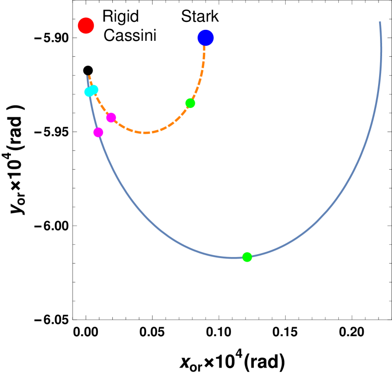
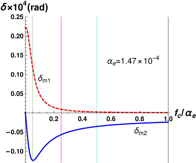
Figure 9: LEFT: Diagram showing average positions of the spin axis of Mercury (normalised to unit norm) projected on the orbital plane. The $\mathbf{e}_{1}$-axis is in the direction of the ascending node of the orbit on the invariable plane and the $\mathbf{e}_{2}$-axis points towards the pole of the invariable plane. This Figure is the analogue of Figure 4 in Baland et al. (2017). The big red point “Rigid Cassini” indicates the position of the spin axis at the Cassini state of the rigid Mercury. The big blue point “Stark” represents the spin orientation at a certain date obtained from observations in Stark et al. (2015), as reported in Baland et al. (2017). Each point on a curve represents the average position of the spin of the mantle $\langle\boldsymbol{\omega}_{m,pr}\rangle$ as given in equation (7.159). The vector from the red-rigid-Cassini point to a point on a curve is the offset that corresponds to that point. The solid-blue curve corresponds to the reference value $k_{c}=\tilde{k}_{c}$ while the dashed-orange curve corresponds to the value $k_{c}=2.5\tilde{k}_{c}$. The value of $f_{c}$ varies from $\tilde{f}_{c}=1.466\times 10^{-4}$ at the black point to zero at the other end of the curve. The points of colours cyan, magenta, and green corresponds to $f_{c}=0.5\tilde{f}_{c}$, $f_{c}=0.25\tilde{f}_{c}$, and $f_{c}=0.05\tilde{f}_{c}$, respectively. For all the range of variation of $f_{c}$, the amplitude of the librations of the mantle ($A$ in equation (7.158)) are less than 3 % of the magnitude of the average offset. RIGHT: The Figure contains the graphs of $f_{c}\to\delta_{m1}$ (dashed-red curve) and $f_{c}\to\delta_{m2}$ (solid-blue curve) for $k_{c}=\tilde{k}_{c}$. The vertical lines correspond to the values of $f_{c}$ of the corresponding coloured points in the figure at the left-hand side.

8 The Chandler wobble period of the Earth and the necessity of complex rheological models.

Our simplified model for the Earth, which ignores the existence of a solid inner core, admits only two modes of torque-free librations: the nearly diurnal free wobble (NDFW) and the Chandler’s wobble. As mentioned in the previous section (see footnote 17) our model cannot provide the correct period of the NDFW. The Chandler wobble period seems to be mostly determined by the rheology of the mantle (paragraph [61] of Mathews et al. (2002)) and not sensitive to other variables, e.g to the deformation of the core-mantle boundary. So, the Chandler’s wobble is within the range of applicability of our model.

The Chandler’s wobble eigenvalue can be estimated using equation (6.136):

$$\begin{split}\lambda_{w}&=i\underbrace{\,\omega\,\frac{{\,\rm I}_{\circ}}{{\rm I}_{\circ m}}\Big{(}\overline{\alpha}_{e}-C(0)\Big{)}}_{:=\sigma_{w}}-\eta_{c}\frac{{\rm I}_{\circ c}}{{\rm I}_{\circ m}}\Big{(}\overline{\alpha}_{e}-C(0)\Big{)}-\tau\omega^{2}C(0)\frac{{\,\rm I}_{\circ}^{2}}{{\rm I}^{2}_{\circ m}}\Big{(}\overline{\alpha}_{e}-C(0)\Big{)}\\ &=\bigg{(}i-E_{k}\frac{{\rm I}_{\circ c}}{{\rm I}_{\circ}}-\tau\omega C(0)\frac{{\,\rm I}_{\circ}}{{\rm I}_{\circ m}}\bigg{)}\sigma_{w}\end{split}$$ (8.170)

where: $\sigma_{w}$ is the Chandler’s wobble frequency, $E_{k}=\eta_{c}/\omega$ is the Ekman number of the flow at the core mantle boundary, and $C(0)=\omega^{2}/(\gamma+\mu_{0})$.

Following Zhang and Shen (2020) we use the following values for the inertial coefficients

$$\frac{{\,\rm I}_{\circ}}{{\rm I}_{\circ m}}=1.13213\qquad\overline{\alpha}_{e}=0.0032845\,.$$

The values of $\gamma$ and $\omega$ for the Earth are given in Table 9 and so, $\sigma_{w}$ is determined by the prestress elastic constant $\mu_{0}$. If we use the value of $\mu_{0}$ provided in Table 9, then we obtain $\sigma_{\omega}=1.90\times 10^{-7}\,sec^{-1}$ that corresponds to the period 382.5 days. This value is far from that obtained from observations ($\approx 433$ days Vondrák et al. (2017)) but it is within the interval (381.9,385) obtained in Mathews et al. (2002) Table 3A.

In Mathews et al. (2002), the explanation for the difference between the estimated frequency and the observed one is that the rheological behaviour of the Earth, encoded in its complex Love numbers, is frequency dependent and the Love number they used to obtain $\sigma_{w}$ was at the diurnal frequency and not at the Chandler wobble frequency. Using our notation, the equation used in Mathews et al. (2002) to obtain the wrong Chandler’s wobble period was $\sigma_{w}=\omega\,\frac{{\,\rm I}_{\circ}}{{\rm I}_{\circ m}}\Big{(}\overline{\alpha}_{e}-C(\omega)\Big{)}$ while, as explained in their Appendix D, they would get the correct period if they had used $\sigma_{w}=\omega\,\frac{{\,\rm I}_{\circ}}{{\rm I}_{\circ m}}\Big{(}\overline{\alpha}_{e}-C(\sigma_{w})\Big{)}$.

The explanation for the failure of our estimate of the Chandler’s wobble period is similar but not the same as that in Mathews et al. (2002). As in ibid., we also calibrated $\mu_{0}$ using the Love number at the diurnal frequency. But we do have a model for the rheology that allows for the variation of the Love number $k(\sigma)$ with the frequency and so, instead of using the approximation $k(\sigma_{w})\approx k(\omega)$, as Mathews et al. (2002) did, we used $k(\sigma_{w})\approx k(0)$, as suggested by the argumentation in Section 6. Our failure occurred because the variation of the Real part of the Love number of the Earth for $\sigma\in(0,\omega)$ is very small when we use the Kelvin-Voigt rheology for the mantle, see Figure 10 left. This is also the reason for us to have obtained the same wrong period for the Chandler’s wobble as Mathews et al. (2002).

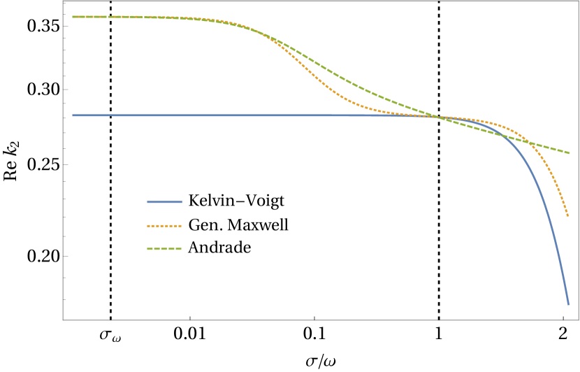
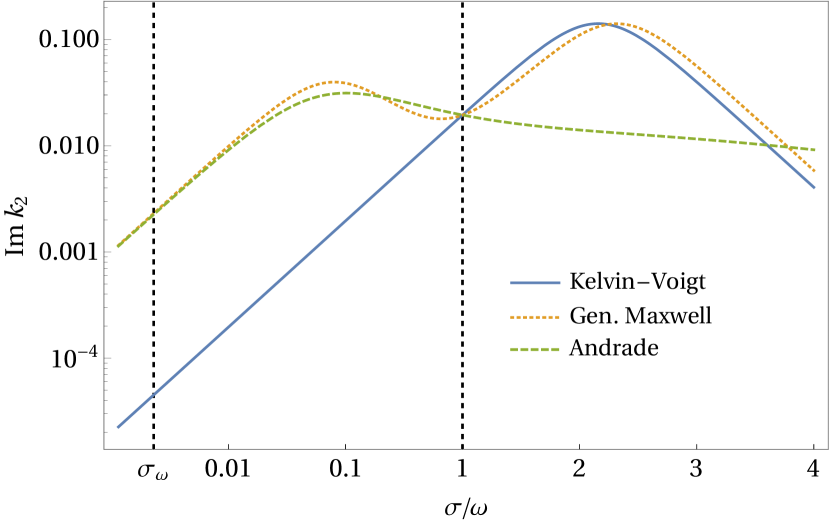
Figure 10: Comparison between the Love number (real part in the left and imaginary part in the right) generated by: a Kelvin-Voigt rheology ($\frac{\mu_{0}}{\omega^{2}}=712\,,\frac{\eta}{\omega}=70.8$), a generalised Maxwell rheology ($\frac{\mu_{0}}{\omega^{2}}=495\,,\frac{\mu_{1}}{\omega^{2}}=219\,,\frac{\eta}{\omega}=49.1\,,\frac{\eta_{1}}{\omega}=2200$), and an Andrade rheology ($\frac{\mu_{0}}{\omega^{2}}=495\,,\frac{\mu_{1}}{\omega^{2}}=728\,,\frac{\eta_{1}}{\omega}=2250\,,\tau_{A}\omega=0.0151\,,\alpha=0.2$). The Kelvin-Voigt model was calibrated with the Love number at diurnal frequency and the generalised Maxwell and the Andrade models were calibrated with the Love number at both diurnal and Chandler’s wobble frequencies. In the left figure and for the Kelvin-Voigt rheology the ratio ${\rm Re}\left(\frac{k(\sigma)}{k(0)}\right)$ decreases from 1 at $\sigma=0$ to $0.995$ at $\sigma=\omega$, which shows that real part of the Love number is almost constant for $\sigma\leq\omega$.

The above argumentation shows that the mantle of the Earth requires a more complex rheological model than that of Kelvin-Voigt. In the following we use two different rheologies to fit the Love numbers at both diurnal and Chandler’s wobble frequencies: a generalised Maxwell rheology with four parameters ($\mu_{0},\eta,\mu_{1},\eta_{1}$) and an Andrade rheology with prestress, for which the complex Love number is

$$k(\sigma)=\frac{3{\,\rm I}_{\circ}G}{R^{5}}\frac{1}{\gamma+\mu_{0}+J_{A}^{-1}(\sigma)}\,,\quad J_{A}(\sigma)=\frac{1}{\mu_{1}}+\frac{1}{i\sigma\eta_{1}}+\frac{\Gamma(1+\alpha)}{\mu_{1}(i\omega\tau_{A})^{\alpha}}\,.$$ (8.171)

If we set $\alpha=0.2$, as in Efroimsky (2012b), then the Andrade rheology will have four free parameters ($\mu_{0},\eta_{1},\mu_{1},\tau_{A}$).

The period of the Chandler’s wobble $\approx 433$ days and equation (6.126) imply that the real part of the Love number at the Chandler’s wobble frequency is approximately $0.358$. If we assume that ${\rm Re}\,k(\sigma_{w})\approx k(0)$, as we did in Section 6, then $C(0)=\frac{\omega^{2}}{\gamma+\mu_{0}}=\frac{\omega^{2}R^{5}}{3{\,\rm I}_{\circ}G}\,k(0)$ implies $\mu_{0}/\omega^{2}=495$. There are several estimates of the real part of $\lambda_{w}$ using observations, here we use ${\rm Re}\,\lambda_{w}=-\sigma_{w}/(2\times Q_{w})$ where $Q_{w}=127$ Nastula and Gross (2015) . If we neglect the contribution of the friction at the CMB to the real part of $\lambda_{w}$, then we can use equation (8.170) to estimate $\tau\omega=\frac{{\rm I}_{\circ m}}{{\,\rm I}_{\circ}}C^{-1}(0)Q_{w}^{-1}/2=2.79$, or $\tau\approx 10.6$ hours.

For the generalised Maxwell model with four parameters ($\mu_{0},\eta,\mu_{1},\eta_{1}$) $\tau=(\eta+\eta_{1})/(\gamma+\mu_{0})$ (equation (6.120)). This relation, the value $\mu_{0}/\omega^{2}=495$, the Love number at the diurnal frequency in Table 8 ($k(\omega)=0.2803-0.01944\,i$), and equation (4.70) imply the values of $\mu_{1}$ and $\eta_{1}$ given in the caption of Figure 10.

For the Andrade model with prestress

$$\tau=\frac{\eta_{1}}{\gamma+\mu_{0}}\,,$$ (8.172)

where $\tau=-\frac{1}{C(0)}\frac{\partial C}{\partial\lambda}(0)$ (equation (6.118)) and $C(\lambda)=\left(\frac{3{\,\rm I}_{\circ}G}{\omega^{2}R^{5}}\right)^{-1}\,k(-i\lambda)$ (equation (6.111)). If we fix $\alpha=0.2$, then a computation similar to that done for the generalised Maxwell model gives the parameter values listed in the caption of Figure 10.

9 Forced libration within the linear approximation.

Formulas for forced librations can be obtained by substitution of the Fourier decomposition of force (known) and angles (unknown) in the linearized equations. In this way the Fourier coefficient of each angle is written as a complex rational function of the forcing frequency. While the numerator of these rational functions depend on the type of forcing, the denominator is always the characteristic polynomial of the homogeneous system. Since the characteristic polynomial can be factored using the eigenvalues, general features of the body response to an external force are determinated by the eigenfrequencies and their associated eigenvectors.

In this Section all the quantitative results are for the Kelvin-Voigt rheology but qualitative aspects of the analysis also apply to other rheologies.

9.1 Rigidity$\times$deformation.

If tidal variations of the total moment of inertia are small compared to the average values, then forced librations are well described by the rigid-mantle approximation. The deformations of the mantle are important in both dissipation of energy and close to resonance frequencies. In Figure 11 we illustrate this fact showing the amplitude of longitude libration of the Moon and of Enceladus as a function of the forcing frequency. We use two rheological models for the mantle: deformable with the Kelvin-Voigt rheology and rigid. The librations are forced by a hypothetical point mass with an almost circular orbit in the equatorial plane of the extended body. If the Jeans operator $\mathbf{S}_{g}$ is written using Stokes variables, then the only terms that appear in the right hand side of equations (5.99) and (5.105) are $s_{22}$ and $c_{20}$. The term $s_{22}$ is proportional to the longitudinal torque and $c_{20}$ acts to flat the body down to the equator, so it does not affect a rigid body.

In Figure 11 (a) we show the amplitude of longitudinal libration of the mantle ($\alpha_{m3}$) for forcing terms of the form $(s_{22},c_{20})=(1,0)\exp(i\chi)$ and $(s_{22},c_{20})=(0,1)\exp(i\chi)$, where $\chi>0$ is the forcing frequency. In the scale of the Figure it is not possible to distinguish between the response function of a body with a deformable mantle from that of a body with a rigid mantle. For the same frequency the angular response to $s_{22}$ is much larger than that to $c_{20}$ (approximately 1000 times larger for the Moon and 200 times for Enceladus). This gives an idea on the relative importance of deformation for forced librations in longitude, since $c_{20}$ affects only a body with a deformable mantle.

In Figures 11 (b), (c), and (d) the forcing term is of the form $(s_{22},c_{20})=(1,0)\exp(i\chi)$. In Figure 11 (b) the domain of variation of $\chi$ is restricted to a small neighbourhood of the resonance frequency of Enceladus. In this domain it is possible to observe the difference between the amplitude of libration of Enceladus with a deformable mantle from that with a rigid mantle. The graphs for the Moon are similar. In Figures 11 (c) and (d) we show the ratio between the amplitude of libration of a body with deformable mantle over that with a rigid mantle. The ratio is very close to one except near the resonant frequency. The rigid mantle approximation is better for the Moon than for Enceladus because the Moon is more rigid.

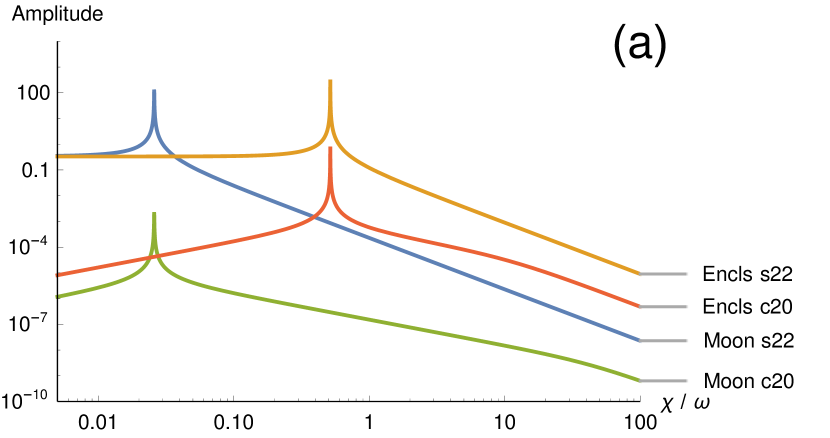
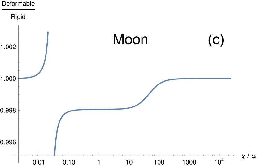
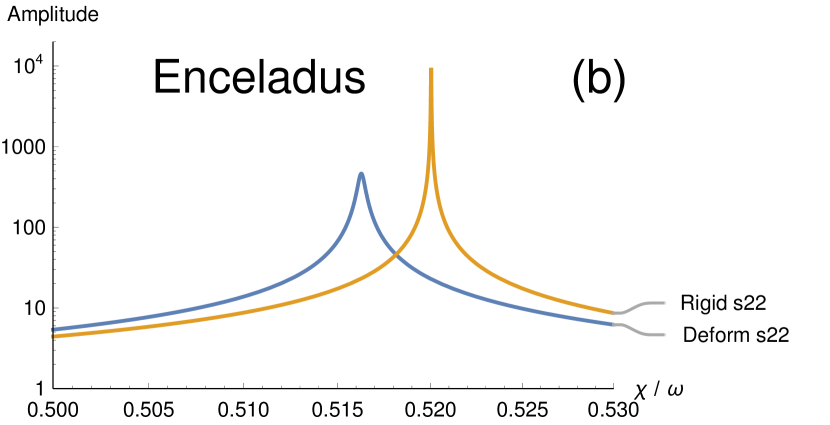
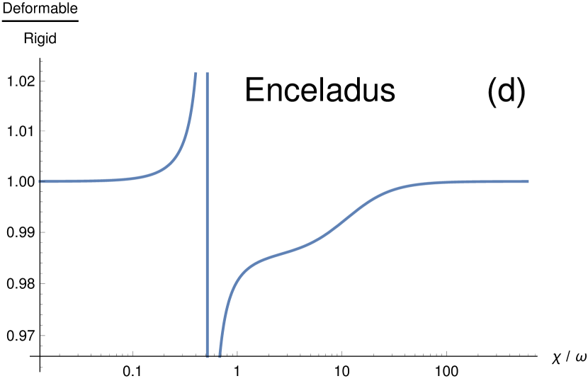
Figure 11: Rigidity$\times$deformation. (a) Amplitude of longitudinal libration of the Moon and Enceladus, both with deformable mantles, for forcing terms of the form $(s_{22},c_{20})=(1,0)\exp(i\chi)$ and $(s_{22},c_{20})=(0,1)\exp(i\chi)$. In Figures (b), (c), and (d) the forcing term is $(s_{22},c_{20})=(1,0)\exp(i\chi)$. (b) Amplitude of longitudinal libration of Enceladus near its resonant frequency ($\approx 0.516\,\omega$): comparison between deformable and rigid mantle. (c) (Moon) and (d) (Enceladus): Ratio between the amplitude of longitudinal libration obtained from a model with deformable mantle over that with rigid mantle. The parameters (Kelvin-Voigt rheology) used to generate the Figure were the following: Moon: $\omega=2.662\times 10^{-6}\,s^{-1},\ f_{0}=0.000700,\ \overline{\alpha}=0.000402,\ \overline{\beta}=0.000636,\ \overline{\gamma}=0.000229,\ f_{c}=0.000158,\ \tau\omega=0.0217,\,\ \eta_{c}/\omega=0.0000158,\ \eta^{-1}\omega=6.99\times 10^{-6}$. Enceladus: $\omega=5.308\times 10^{-5}\,s^{-1},\ f_{0}=3.96,\ \overline{\alpha}=0.00707,\ \overline{\beta}=0.0254,\ \overline{\gamma}=0.0183,\ f_{c}=0.0161,\ \tau\omega=0.0889,\,\ \eta_{c}/\omega=0.0000320,\ \eta^{-1}\omega=0.000985$.

9.2 Eigenmodes and forced librations.

The phase space of a forced linear system with constant coefficients can be decomposed into eigenspaces of the homogeneous system. If the forcing terms are decomposed into eigenspace components, then the forced linear system decouples into a system of independent oscillators, one for each eigenmode. The geometry of the oscillations in a particular eigenmode is determined by the respective eigenvectors.

The idea in the previous paragraph can be applied to the rotational eigenmodes of Section 6 with caution, as we now explain. In the computation of the rotational eigenvalues and eigenvectors we were able to reduce all the information in the internal variables of the rheology (represented by extensions of the springs and dash-pots of their representation) into the Love number and the deformation variables $\boldsymbol{\delta}\mathbf{B}$. In this way we were able to compute the $\boldsymbol{\alpha}_{m}$, $\boldsymbol{\alpha}_{c}$, and $\boldsymbol{\delta}\mathbf{B}$ without having to compute the components associated with the internal variables. This approximation is good close to the frequencies of the free eigenmodes, namely at low frequencies for the libration in longitude and wobble modes and close to the diurnal frequency for the nearly diurnal free wobble and librations in latitude modes. For forced librations where the forcing frequency is far from the natural frequencies the part of the eigenvectors that depends of the internal variables may be relevant. In the following discussion we will disregard this issue.

Libration in longitude are oscillations in the two dimensional eigenspace associated with the eigenvector in equation (6.135). The ratio between the $\beta_{3}$-component and the $\alpha_{m3}$-component of this eigenvector is $\beta_{3}/\alpha_{m3}=-\frac{C(0)}{\overline{\gamma}}(\xi_{2}-\xi_{1})$. As shown in Figure 5 (Right), $\beta_{3}(t)$ is the angle, measured in the plane orthogonal to $\mathbf{e}_{3}\in\mathrm{K}_{m}$, between the $I_{1}$-principal axis of the deformable body and its average position, which is the $\mathbf{e}_{1}$-axis of $\mathrm{K}_{m}$ (the prestress frame). So, $|\beta_{3}/\alpha_{m3}|=\frac{C(0)}{\overline{\gamma}}(\xi_{2}-\xi_{1})$ gives the relative importance of deformation in longitudinal librations. The same idea can be applied to the other rotational modes.

9.3 Parametric Resonances: limitations of the forced libration model.

In our derivation of the linearized equations we assumed the hypothesis (5.87): The effect of $[\boldsymbol{\delta}\mathbf{J}_{g}\,,\boldsymbol{\widehat{\alpha}}_{m}]$ is negligible. In some situations an averaging procedure justifies this assumption. The convenience of this hypothesis is that the homogeneous linearized equations for librations are of constant coefficients and the analysis of their solutions is easy. The drawback of this approach is that it prevents the occurrence of parametric resonances.

The equations for free librations with constant coefficients, on the contrary to those for forced librations, are useful even when $[\boldsymbol{\delta}\mathbf{J}_{g}\,,\boldsymbol{\widehat{\alpha}}_{m}]$ is not negligible. Indeed, if $\lambda=i\omega_{0}+\nu_{0}$ is an eigenvalue of the equation with constant coefficients, then parametric resonances may occur for forcing frequencies $\chi$ that satisfy: $\omega_{0}/\chi\approx j/2$, $j=1,2,\ldots$. So, the eigenfrequencies of the equations with constant coefficients determine the parametric-resonance frequencies. Note that even a small dissipation of energy, $\nu_{0}>0$, may have an effect on preventing the parametric resonance to occur, specially for large values of $j$ (see, e.g., Arnold (1992)).

10 The Moon in INPOP and in JPL ephemerides

In the main international ephemerides, the Moon is assumed to be composed of a homogeneous liquid core surrounded by a prestressed viscoelastic mantle. This model that we will call INPOP19a was the main motivation for the present paper. The geometry of the Moon’s core cavity is fixed and the tidal response of the viscoelastic mantle is represented by the constant time lag model Fienga et al. (2019) Viswanathan et al. (2019), (Folkner et al., 2014), and Park et al. (2021). The INPOP19a is formally equivalent to the model we presented in Section 5, equations (5.77) and (5.78), except for the gravitational modulus $\gamma$ and for the fact that INPOP19a incorporate additional physical effects, as for instance figure-figure torques and higher order gravitational moments. Since $\gamma$ appears always added to $\mu_{0}$ and for the Moon self-gravity seems to be much less important than elastic rigidity $\mu_{0}\gg\gamma$, in the following we set $\gamma=0$.

10.1 INPOP19a parameters

The parameters used in INPOP19a are summarised in Table 10. They are related to the parameters of the present model as follows

$$\frac{{\rm I}_{\circ,T}}{\mathcal{M}\mathcal{R}_{T}^{2}} = \frac{C_{T}}{\mathcal{M}\mathcal{R}_{T}^{2}}+\frac{2}{3}C_{20T}\,,$$ (10.174)

$$\frac{{\rm I}_{\circ,c}}{\mathcal{M}\mathcal{R}_{T}^{2}} = \frac{C_{c}}{\mathcal{M}\mathcal{R}_{T}^{2}}+\frac{2}{3}C_{20c}\,,$$ (10.175)

$$\frac{{\rm I}_{\circ,m}}{\mathcal{M}\mathcal{R}_{T}^{2}} = \frac{{\rm I}_{\circ,T}}{\mathcal{M}\mathcal{R}_{T}^{2}}-\frac{{\rm I}_{\circ,c}}{\mathcal{M}\mathcal{R}_{T}^{2}}\,,$$ (10.176)

$$\mathbf{B}_{0}(0) = \frac{2}{3}\frac{\mathcal{M}\mathcal{R}_{T}^{2}}{{\rm I}_{\circ,T}}\begin{bmatrix}3C_{22T}-\frac{1}{2}C_{20T}&0&0\\ 0&-3C_{22T}-\frac{1}{2}C_{20T}&0\\ 0&0&C_{20T}\end{bmatrix}$$

$$+ \frac{n^{2}}{3\mu_{0}}\begin{bmatrix}-1&0&0\\ 0&-1&0\\ 0&0&2\end{bmatrix}=\mathbf{B}_{0,m}\ ,$$

$$\mathbf{B}_{c}(0) = \frac{2}{3}\frac{\mathcal{M}\mathcal{R}_{T}^{2}}{{\rm I}_{\circ,c}}\begin{bmatrix}-\frac{1}{2}C_{20c}&0&0\\ 0&-\frac{1}{2}C_{20c}&0\\ 0&0&C_{20c}\end{bmatrix}=\mathbf{B}_{c,m}\,\ ,$$ (10.178)

$$\mu_{0} = 3\frac{\mathcal{G}\mathcal{M}_{\mathrm{EMB}}}{1+EMRAT}\frac{{\rm I}_{\circ,T}}{\mathcal{M}\mathcal{R}_{T}^{2}}\frac{1}{\mathcal{R}^{3}_{T}\,k_{2}}\,,$$ (10.179)

$$\eta = \mu_{0}\tau_{M}\,,$$ (10.180)

$$\bar{k}_{c} = \frac{k_{c}}{C_{T}}\frac{C_{T}}{\mathcal{M}\mathcal{R}_{T}^{2}}\frac{\mathcal{M}\mathcal{R}_{T}^{2}}{{\rm I}_{\circ,T}}\,,$$ (10.181)

$$\mathbf{F} = -\left(\boldsymbol{\omega}_{m}\otimes\boldsymbol{\omega}_{m}-\frac{\omega_{m}^{2}}{3}\mathbb{I}\right)+3\frac{\mathcal{G}\mathcal{M}_{\mathrm{EMB}}}{1+1/EMRAT}\frac{1}{r^{5}}\left(\mathbf{r}\otimes\mathbf{r}-\frac{r^{2}}{3}\mathbb{I}\right)\,.$$

Table 10: Parameters taken from INPOP19a Fienga et al. (2019).

Parameter	Notation	Value	Unit
Earth-Moon mass ratio	$\qquad{}EMRAT\qquad{}$	81.300 566 772 76764
Gravitational mass of E-M barycenter	$\mathcal{G}\mathcal{M}_{\mathrm{EMB}}$	$\quad{}8.997\,011\,394\,021\,228\times 10^{-10}\quad{}$	au3/day2
Lunar time delay for tide	$\tau_{M}$	$0.094\,332\,332\,227\,022\,27$	day
Lunar potential Love number	$k_{2}$	$0.023\,559$
Polar moment of inertia of the Moon	$C_{T}/\mathcal{M}\mathcal{R}^{2}_{T}$	$0.393\,140\,294\,559\,018$
Polar moment of inertia of the core	$C_{c}/\mathcal{M}\mathcal{R}^{2}_{T}$	$0.000\,275$
Lunar gravity field	$C_{20T}$	$-0.000\,203\,212\,558\,851\,8901$
—	$C_{22T}$	$2.238\,295\,071\,767\,246\times 10^{-5}$
Lunar core gravity field	$C_{20c}$	$-4.342\,243\,760\,334\,537\times 10^{-8}$
—	$C_{22c}$	0
Coefficient of viscous friction at CMB	$k_{c}/C_{T}$	$6.443\,479\,383\,181\,008\times 10^{-9}$	rad/day
Lunar radius	$\mathcal{R}_{T}$	1738	km
Astronomical unit	au	149 597 870.7	km

10.2 Comparison between INPOP19a and our model.

In this section we integrate numerically equations (5.77) and (5.78) to compute the librations of the Moon forced by the Earth and the Sun. The positions of the Earth and the Sun relative to the Moon were obtained from the orbits of the Earth and Moon as given in Yoder (1995) (Table 4a). The parameterization of the orbits is that in equation (A.183) with $r=\left(\frac{a_{p}(1-e^{2})}{1+e\cos f}\right)$ and

$$f=M_{p}+e\left(2-\frac{1}{4}e^{2}\right)\sin M_{p}+\frac{5}{4}e^{2}\sin 2M_{p}+\frac{13}{12}e^{3}\sin 3M_{p}+\mathcal{O}(e^{4}).$$ (10.182)

In Figure 12, we plot the first and second components of the angular velocity of the mantle $\boldsymbol{\omega}_{m,m}/|\boldsymbol{\omega}_{m,m}|$ and of the Tisserand angular velocity of the whole Moon $\boldsymbol{\omega}_{T,m}/|\boldsymbol{\omega}_{T}|$. As expected, the mantle angular velocity has a larger amplitude of oscillations.

In Figure 13 - Left, we plot $\boldsymbol{\omega}_{m,m}/|\boldsymbol{\omega}_{m,m}|$ using the data from INPOP19a (the data for the Figure was generously provided by Prof. Herve Manche). In the figure generated with the INPOP19a data the oscillations of $\boldsymbol{\omega}_{m}$ are centred at the point $(-0.0004,0)$ while in Figure 12 the oscillations are symmetric with respect to the origin. This discrepancy lead us to investigate the role played by a possible small tilt of the symmetry axis of the core with respect to the $\mathbf{e}_{3}$-axis of $\mathrm{K}_{m}$. In Figure 13 - Right we show that the same offset obtained with the INPOP19a data can be obtained from our model if we set the tilt equal to $0.325^{\circ}$, see Figure 14 . As pointed out by Prof. V. Viswanathan (personal communication), the offset observed in INPOP19a does not come from any tilt of the core cavity with respect to the mantle frame but from other physical effects which were not taken into account in our model, e.g. higher order gravitational moments.

Figures 12 and 13 show that the agreement between the results obtained with INPOP19a and those obtained with our model is excellent, except for the offset of the centre of libration of $\boldsymbol{\omega}_{m,m}$ that in INPOP19a is due to physical effects not taken into account in our model.

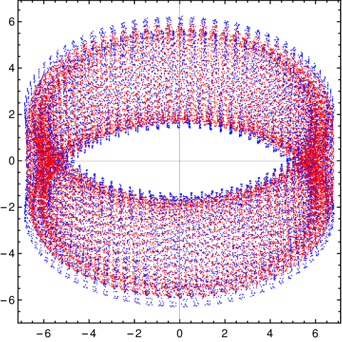
Figure 12: Path of the normalised angular velocity vector $(\omega_{1},\omega_{2})/|\boldsymbol{\omega}|$ ($\times 10^{-4}$) in the $(\mathbf{e}_{1},\mathbf{e}_{2})-$plane of $\mathrm{K}_{m}$, $\boldsymbol{\omega}_{m}$ (blue) and $\boldsymbol{\omega}_{T}$ (red).

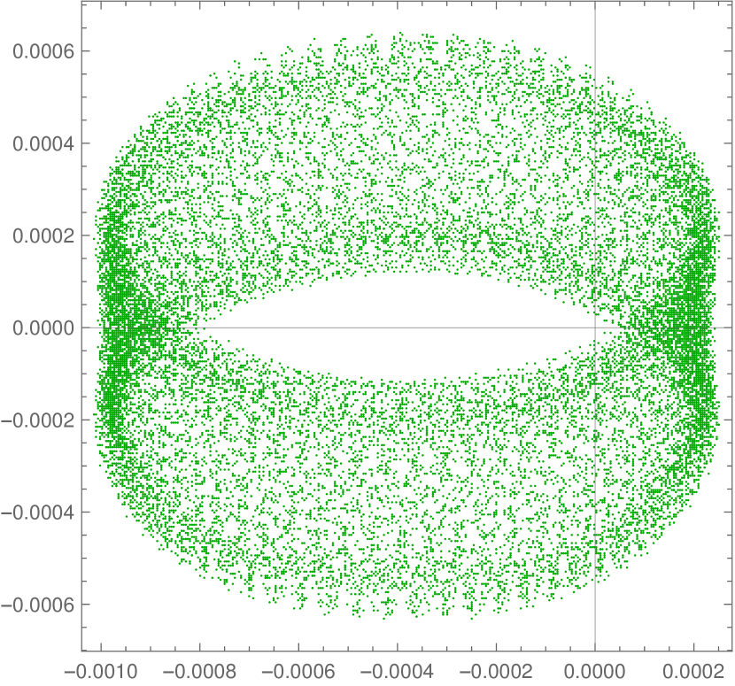
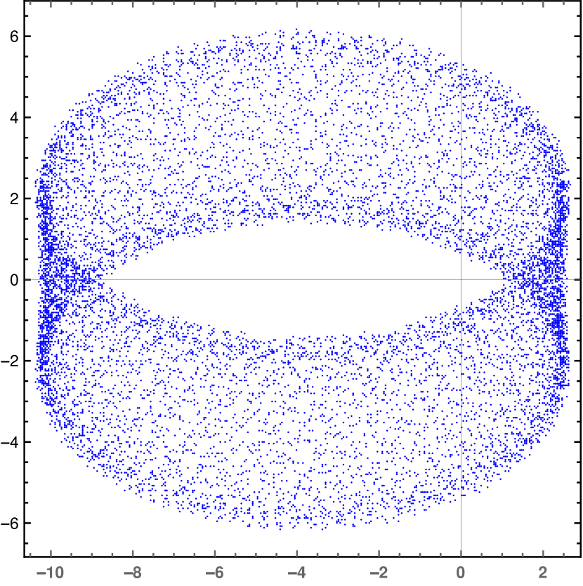
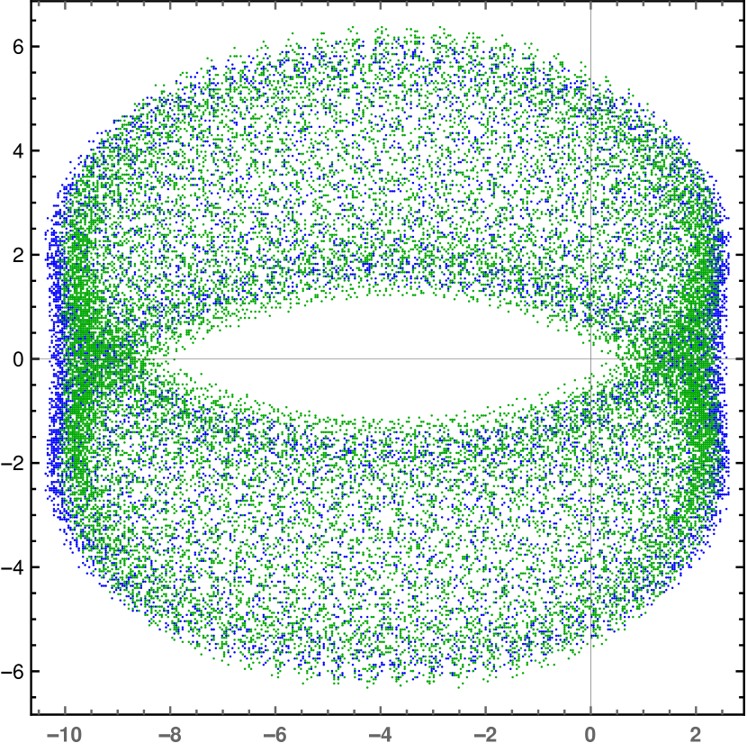
Figure 13: Path of the normalised angular velocity vector $(\omega_{m,m1},\omega_{m,m2})/|\boldsymbol{\omega}_{m}|$ ($\times 10^{-4}$): Left INPOP19a, Center our model with a tilted core cavity, as illustrated in Figure 14, and Right superposition of both plots INPOP19a (green) and our model with a tilted cavity (blue).

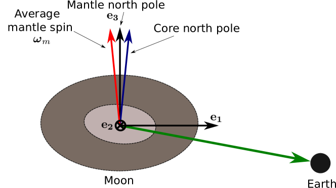
Figure 14: Inclination between the symmetry axis of the core cavity and the mantle frame $\mathrm{K}_{m}$.

11 Conclusions

The main result in this paper is the set of equations (5.77), for the librations of a body made of a mantle and a fluid core, and either equation (5.78), or (5.79), or (5.80), for the deformations of the mantle. The equations for the deformations are so general that the mantle can have essentially any linear viscoelastic rheology (models with infinite memory, as the Andrade, can be approximated with arbitrary accuracy Gevorgyan et al. (2020)). While the (rigid) inertial part of these equations is well known and the deformation part already appeared in Ragazzo and Ruiz (2017), the combination of the two parts is new.

In Section 4 we introduced the important concept of prestress frame. There is an old idea that part of the deformation of bodies out of hydrostatic equilibrium is due to an almost static transient state associated with a large viscosity of the mantle (fossil deformation). We reformulated this idea mathematically using rheological models of bodies that in the absence of external forces eventually become spherical. With this concept we linked the triaxiality of the body to the parameters of the rheology, equation (4.60), and we separated the time scale of the librations (years) from the time scale of variations of the triaxiality (thousands of years or more). Our point is: fossil deformation, being correct or not, provides a physical argument to be used in the theory of spherically symmetric bodies, on which we are confident in, to build a mathematical model to describe the librations of slightly aspherical bodies out of hydrostatic equilibrium.

Most of the present paper is related to the validation of our equations for the librations. In order to do this, in Section 6, we present equations for the rotational eigenvalues and eigenvectors of free librations. These equations apply to both bodies in and out-of spin orbit resonance and are formulated in terms of Love numbers, so they are independent on the rheological model used for the mantle. We are not aware of other formulas for free librations with such level of generality, including our definition of the characteristic time $\tau$ in equation (6.118) that does not depend on the choice of a rheological model. In particular cases our formulas agree with others found in the literature. We summarised and illustrated all our results about free librations in Section 6.4.

Another important result in this paper are the formulas for the inertial offsets, in particular that in equation (7.166) for a body in s-to-2 spin-orbit resonance. This formula is new and may be particularly useful in the estimation of the core parameters $k_{c}$ and $f_{c}$.

Some of our formulas for the eigenvalues of free librations, e.g. (C.215) and (C.216), are quite complicated. If other features are included to the model; as for instance, a solid core, deformation of the fluid cavity, and core-mantle-magnetic coupling; then these formulas will probably become much more complicated. In this case the analytical treatment of the problem may be doable but not elucidative. In contrast, the model for librations we presented in this paper is quite simple and the addition of few other effects, by means of the Lagrangian formalism, will not complicate it a lot. So, we conclude that the most promising approach to the libration problem is the numerical simulation of models with a minimum of physical parameters that can be calibrated directly from observations (see, e.g., Noyelles (2018)).

Appendix A The value of the coefficients $c_{1},c_{2},c_{3}$ in equation (2.23) for a body in a Cassini state.

The theoretical determination of the almost equilibrium orientation of the spin axis of an extended body, or the guiding motion as described in Section 2, is a difficult task that requires some knowledge about the rheological behaviour of the body. An important situation, which will be the one considered in this appendix, is that of a rigid body under the influence of a single point mass that moves according to a Keplerian precessing orbit. In this case the guiding motion is called “a Cassini state” Peale (1969). We remark that different Cassini states can be obtained under different rheological hypotheses (see, for instance, Boué (2020) for bodies with a rigid mantle and a fluid core).

Let $\kappa$ be the inertial frame and $\mathrm{K}_{g}$ be the guiding frame described in Section 2. We recall that the common origin of both frames is the centre of mass of the extended body. The position of the point mass with respect to the extended body in the frame $\kappa$ is given by

$$\mathbf{r}=\mathbf{R_{3}}(\Omega_{p})\mathbf{R_{1}}(\iota_{p})\mathbf{R_{3}}(\omega_{p})\begin{bmatrix}r\cos(f_{p})\\ r\sin(f_{p})\\ 0\end{bmatrix}$$ (A.183)

where: $\iota_{p}$, $f_{p}$, $\omega_{p}$, and $\Omega_{p}$ are the inclination with respect to an invariable plane (the “Laplace plane”), the true anomaly, the argument of the periapsis and the longitude of the ascending node, respectively, of a classical Keplerian orbit that has semi-major axis $a_{p}$, eccentricity $e$, and mean anomaly $M_{p}$ (the index $p$ stands for point-mass).

We recall that the three axes of $\mathrm{K}_{g}$ are those of the body’s principal moments of inertia, $\overline{I}_{1}<\overline{I}_{2}<\overline{I}_{3}$, in the absence of deformation. The orientation of the guiding frame $\mathbf{R_{g}}:\mathrm{K}_{g}\to\kappa$ is given by three Euler angles

$$\mathbf{R_{g}}=\mathbf{R_{3}}(\psi_{g})\mathbf{R_{1}}(\theta_{g})\mathbf{R_{3}}(\phi_{g})$$ (A.184)

where: $\theta_{g}$ is the inclination of the body equator to the Laplace plane, $\psi_{g}$ is the longitude of the ascending node of the body equator, and $\phi_{g}$ is the angle between the ascending node and Axis 1. There are two possible orientations of Axis 1, so $\mathbf{R}_{g}$ is not uniquely defined. In the case of the Moon it is usual to choose the positive orientation of Axis 1 as that pointing towards the Earth (see, e.g., Eckhardt, 1981). To change from one orientation to the other it is enough to change the signs of both unit vectors $\mathbf{e}_{1}$ and $\mathbf{e}_{2}$.

The orientation of the slow frame is given by $\mathbf{R}_{s}(t)=\mathbf{R}_{g}(t)\mathbf{R_{3}}^{-1}(\omega\,t):\mathrm{K}_{s}\to\kappa$, equation (2.14), that in the present case becomes

$$\mathbf{R}_{s}=\mathbf{R_{3}}(\psi_{g})\mathbf{R_{1}}(\theta_{g})\mathbf{R_{3}}(\zeta)\quad\text{where}\quad\zeta=\phi_{g}-\omega t\,.$$ (A.185)

The identity $\langle\boldsymbol{\omega}_{s,g}\,,\mathbf{e}_{3}\rangle=0$ implies

$$\dot{\zeta}=-\dot{\psi}_{g}\cos\theta_{g}\,.$$ (A.186)

The position of the point mass in the guiding frame $\mathrm{K}_{g}$ is given by $\mathbf{r_{g}}=\mathbf{R_{g}}^{-1}\mathbf{r}$ and equations (A.183) and (A.184) imply

$$\mathbf{r_{g}}=r\Big{(}\cos\big{(}f_{p}\big{)}\mathbf{u}+\sin\big{(}f_{p}\big{)}\mathbf{v}\Big{)}$$ (A.187)

where $\mathbf{u}$ and $\mathbf{v}$ are the first and second columns, respectively, of the matrix $\mathbf{R_{g}}^{-1}\mathbf{R_{3}}(\Omega_{p})\mathbf{R_{1}}(\iota_{p})\mathbf{R_{3}}(\omega_{p})$. The force matrix in the guiding frame $\mathbf{J}_{g}$, as defined in Section 2, is given by

$$\begin{split}&J_{gij}=\bigg{(}\frac{3{\cal G}m_{p}}{|\mathbf{r_{g}}|^{5}}\mathbf{r_{g}}\otimes\mathbf{r_{g}}\bigg{)}_{ij}\\ &\ \quad=\frac{3{\cal G}m_{p}}{2r^{3}}\bigg{(}\big{(}u_{i}u_{j}+v_{i}v_{j}\big{)}+\cos\big{(}2f_{p}\big{)}\big{(}u_{i}u_{j}-v_{i}v_{j}\big{)}+\sin\big{(}2f_{p}\big{)}\big{(}u_{i}v_{j}+v_{i}u_{j}\big{)}\bigg{)}\,.\end{split}$$ (A.188)

Notice that the vectors $\mathbf{u}$ and $\mathbf{v}$ in equation (A.187) are the rows of an orthogonal matrix, which implies $|\mathbf{u}|=|\mathbf{v}|=1$ and $\langle\mathbf{u},\mathbf{v}\rangle=0$. So,

$$\operatorname{Tr}\mathbf{J}_{g}=\frac{3{\cal G}m_{p}}{r^{3}}\,.$$ (A.189)

Now we impose that the extended body is in a Cassini state that is characterised by three laws Colombo (1966), Peale (1969), Peale (1974), which are generalisations of the original laws of Cassini (1693) (aimed to describe the motion of the Moon, see Eckhardt (1981)).

• The body spin is in $s$-to-2 resonance with the orbital mean motion, where $s$ is a positive integer (for the Moon $s=2$ and for Mercury $s=3$);

• The inclination of the body equator $\theta_{g}$ with respect to the Laplace plane is constant;

• Either the ascending node (state 1) or the descending node (state 2) of the body equator on the Laplace plane precesses in coincidence with the ascending node of the orbit on the Laplace plane (the spin axis, orbit normal, and Laplace plane normal are coplanar).

The third law implies that either

$$\begin{array}[]{rll}\psi_{g}&=\Omega_{p}&\text{state 1 (e.g. Mercury) or}\\ \psi_{g}&=\Omega_{p}+\pi&\text{state 2 (e.g. Moon),}\end{array}$$ (A.190)

then the second law implies that the inclination of the body spin axis with respect to the normal to the orbital plane, given by ($\theta_{g}\geq 0$, $\iota_{p}\geq 0$)

$$\begin{array}[]{rll}\chi_{p}&=\theta_{g}-\iota_{p}\geq 0&\text{state 1}\\ \chi_{p}&=\theta_{g}+\iota_{p}&\text{state 2}\end{array}$$ (A.191)

is constant (the inequality in state 1 is of dynamical origin, see Peale (1969) paragraph below equation (18)); and then the first law implies that $sM_{p}=2(\phi_{g}-\omega_{p})$ .

For a body in a Cassini state 2 (e.g. Moon) equation (A.187) becomes

$$\mathbf{r_{g}}=r\cos f_{p}\underbrace{\begin{bmatrix}-\cos\phi_{g}\cos\omega_{p}-\cos\chi_{p}\sin\phi_{g}\sin\omega_{p}\\ \cos\omega_{p}\sin\phi_{g}-\cos\phi_{g}\cos\chi_{p}\sin\omega_{p}\\ \sin\chi_{p}\sin\omega_{p}\end{bmatrix}}_{\mathbf{u}}+r\sin f_{p}\underbrace{\begin{bmatrix}-\cos\chi_{p}\cos\omega_{p}\sin\phi_{g}+\cos\phi_{g}\sin\omega_{p}\\ -\cos\phi_{g}\cos\chi_{p}\cos\omega_{p}-\sin\phi_{g}\sin\omega_{p}\\ \cos\omega_{p}\sin\chi_{p}\end{bmatrix}}_{\mathbf{v}}$$ (A.192)

and for a body in a Cassini state 1 we must replace $\mathbf{u}\to-\mathbf{u}$ and $\mathbf{v}\to-\mathbf{v}$. Since $J_{gij}$ given in equation (A.188) depends only on the products of components of $\mathbf{u}$ and $\mathbf{v}$, the matrix $\mathbf{J}_{g}$ has the same expression for both states 1 and 2. Therefore, the following computation of $c_{1}$, $c_{2}$ and $c_{3}$ holds in both cases.

The coefficients $c_{1},c_{2},$ and $c_{3}$ we aim to compute are determined by the constant term in the Fourier expansion of $J_{gij}$ given in equation (A.188). In order to compute the Fourier expansion of the factors involving $r$ and $f_{p}$ we use the Hansen coefficients defined by

$$\bigg{(}\frac{r}{a_{p}}\bigg{)}^{n}{\rm e}^{imf}=\sum_{k=-\infty}^{\infty}X^{n,m}_{k}(e){\rm e}^{ikM}$$ (A.194)

The computation of the coefficients $c_{1},c_{2},$ and $c_{3}$ in equation (2.23) can be done in the following way. At first we use equation (A.189) to obtain

$$c_{3}=\frac{{\cal G}m_{p}}{\omega^{2}a_{p}^{3}}X_{0}^{-3,0}(e)\,.$$ (A.195)

The term $\left(\frac{3{\cal G}m_{p}}{\omega^{2}|\mathbf{r_{g}}|^{5}}\mathbf{r_{g}}\otimes\mathbf{r_{g}}\right)_{33}$ can be easily computed using equations (A.188) and (A.194) and the result is $\frac{3{\cal G}m_{p}}{2\omega^{2}a_{p}^{3}}X_{0}^{-3,0}(e)\sin^{2}(\chi_{p})=c_{3}-2c_{1}/3$. So, we obtain that

$$c_{1}=\frac{3\,{\cal G}m_{p}}{2\,\omega^{2}a_{p}^{3}}X_{0}^{-3,0}(e)\bigg{(}1-\frac{3}{2}\sin^{2}(\chi_{p})\bigg{)}\,.$$ (A.196)

In order to compute the constant $c_{2}$ associated with an $s-to-2$ spin-orbit resonance it is enough to compute the constant term in the Fourier expansion of $\left(\frac{3{\cal G}m_{p}}{\omega^{2}|\mathbf{r_{g}}|^{5}}\mathbf{r_{g}}\otimes\mathbf{r_{g}}\right)_{11}$ and then to use that this term is equal to $c_{1}/3+c_{2}+c_{3}$, equation (2.23). Assuming that the precession of the periapsis is different from zero a computation gives

$$c_{2}=\frac{3\,{\cal G}m_{p}}{2\,\omega^{2}a_{p}^{3}}X_{s}^{-3,2}(e)\cos^{4}(\chi_{p}/2)$$ (A.197)

Another case of interest is that of a point mass that moves in a precessing Keplerian orbit, as that parameterised in equation (A.183), with constant inclination, $\iota_{p}=$constant, and with no spin-orbit resonance. By no spin-orbit resonance we mean that the constant frequencies $\dot{\psi}_{g}$, $\dot{\Omega}_{p}$, $\omega$, $\dot{\omega}_{p}$, and $\dot{M}$ are noncomensurable. Equation (A.189) implies that $c_{3}$ is again given by equation (A.195) and the condition of no spin-orbit resonance implies $c_{2}=0$. As before, to compute $c_{1}$ we look for a term in $J_{g33}$ that is constant in time. Using that $X^{-3,\pm 2}_{0}=0$ and the no spin-orbit hypothesis we obtain that

$$\frac{3{\cal G}m_{p}}{2r^{3}}\bigg{(}\cos\big{(}2f_{p}\big{)}\big{(}u_{3}^{2}-v_{3}^{2}\big{)}+\sin\big{(}2f_{p}\big{)}2u_{3}v_{3}\bigg{)}$$

does not contain any term that is constant. Using that $-\dot{\psi}_{g}+\dot{\Omega}_{p}\neq 0$, an analysis of the remaining term, $\frac{3{\cal G}m_{p}}{2r^{3}}\big{(}u_{3}^{2}+v_{3}^{2}\big{)}$, shows that the constant term of $J_{g33}$ is

$$\frac{3{\cal G}m_{p}}{2a_{p}^{3}}X^{-3,0}_{0}\frac{1}{8}\Big{(}-\cos(2\theta_{g})-(3\cos(2\theta_{g})+1)\cos(2\iota_{p})+5\Big{)}=\omega^{2}\left(c_{3}-\frac{2}{3}c_{1}\right)$$

So, using equation (A.195) for $c_{3}$ we obtain that for no spin-orbit resonance:

$$\begin{split}c_{1}&=\frac{3{\cal G}m_{p}}{\omega^{2}a_{p}^{3}}X^{-3,0}_{0}\frac{1}{32}\Big{(}3\cos(2\theta_{g})+1\Big{)}\Big{(}3\cos(2\iota_{p})+1\Big{)}\\ c_{2}&=0\end{split}$$ (A.198)

If there are several point masses, $\beta=1,2,\ldots$, orbiting the extended body, each one in a precessing Keplerian orbit, with constant inclination, $\iota_{\beta}=$constant, and with no spin-orbit resonance; as in the case where the Earth is the extended body and the Moon and the Sun represent the point masses; then $c_{2}=0$ and (the index $p$ was omitted in several constants)

$$c_{1}=\bigg{(}\sum_{\beta}s_{\beta}\bigg{)}\frac{1+3\cos(2\theta_{g})}{4}\quad\text{where}\quad s_{\beta}=\frac{3{\cal G}m_{\beta}}{\omega^{2}a_{\beta}^{3}}(1-e_{\beta}^{2})^{-3/2}\,\frac{1+3\cos(2\iota_{\beta})}{8}\,.$$ (A.199)

In this case the average rate of precession $\dot{\psi}_{g}$ of the spin axis of the extended body is Williams (1994):

$$\frac{\dot{\psi}_{g}}{\omega}=-\big{(}\sum_{\beta}s_{\beta}\big{)}\frac{\overline{I}_{3}-\overline{I}_{e}}{\overline{I}_{3}}\cos\theta_{g}\approx-\big{(}\sum_{\beta}s_{\beta}\big{)}\overline{\alpha}_{e}\,\cos\theta_{g}\,;$$ (A.200)

and the motion of the slow frame is determined by $\mathbf{R}_{s}$ as given in equations (A.185) and (A.186) with $\theta_{g}=$constant.

Appendix B A simple model: Considerations about the guiding frame.

In this appendix we show by means of an example how the inertial forces that appear due to the non-inertial character of the guiding frame are mostly cancelled out by external torques. This example will be used in Appendix E.

The problem is to describe the axial precession of an extended rigid body of mass $m$ and moment of inertia $\mathbf{I}$ under the gravitational force of a point of mass $m_{p}$ that moves in a circular orbit of radius $a_{p}$ and with angular frequency $n$. We assume that the body is axisymmetric with $\overline{I}_{1}=\overline{I}_{2}=\overline{I}_{e}<\overline{I}_{3}$. We define a body frame $\mathrm{K}$ such that the $\mathbf{e}_{3}$-axis is the $\overline{I}_{3}$-principal axis and an inertial frame $\kappa$ such that the orbit of the point mass has components $(a_{p}\cos(nt),a_{p}\sin(nt),0)$.

Let $\omega>0$ be the initial spin angular speed of the body that is defined as the projection of the initial angular velocity vector $\boldsymbol{\omega}$ on the $I_{3}$-principal axis. We assume that the angular velocity is almost aligned with the $I_{3}$-principal axis and that inertial forces prevail over the gravitational torque, namely

$$\omega/\|\boldsymbol{\omega}\|\approx 1\quad\text{and}\quad\frac{3}{2}\frac{Gm_{p}}{\omega^{2}a^{3}}=s\ll 1$$ (B.201)

In this case the torque-free inertial motion dominates and the body rotates almost steadily about the spin-axis. Note that $s$ is the quantity that we denoted as $s_{\beta}$ in equation (A.199).

The tidal-force operator $\mathbf{J}=\frac{3{\cal G}m_{p}}{r^{5}}\mathbf{r}\otimes\mathbf{r}$ can be decomposed into two terms

$$\mathbf{J}=\underbrace{s\,\omega^{2}\left(\begin{array}[]{ccc}1&0&0\\ 0&1&0\\ 0&0&0\\ \end{array}\right)}_{=\mathbf{J}_{0}}+\underbrace{s\,\omega^{2}\left(\begin{array}[]{ccc}\cos(2nt)&\sin(2nt)&0\\ \sin(2nt)&-\cos(2nt)&0\\ 0&0&0\\ \end{array}\right)}_{=\mathbf{J}_{1}}\,.$$ (B.202)

The axial precession is determined by the constant part $\mathbf{J}_{0}$, so in the following we consider the problem of the motion of the extended body only under tidal-force operator $\mathbf{J}_{0}$, namely

$$\begin{split}&\dot{\boldsymbol{\widehat{\pi}}}=[\mathbf{I}\,,\mathbf{J}_{0}]\quad\text{where}\quad\mathbf{R}:\mathrm{K}\to\kappa\\ &\boldsymbol{\widehat{\pi}}={\rm\!\ Tr\!\ }\big{(}\mathbf{I}\big{)}\boldsymbol{\widehat{\omega}}-\mathbf{I}\boldsymbol{\widehat{\omega}}-\boldsymbol{\widehat{\omega}}\mathbf{I}\,,\quad\boldsymbol{\widehat{\omega}}=\dot{\mathbf{R}}\mathbf{R}^{-1}\,.\\ \end{split}$$ (B.203)

A computation shows that $\mathbf{R}=\mathbf{R}_{3}(\dot{\psi}\,t)\mathbf{R}_{1}(\theta)\mathbf{R}_{3}(-\dot{\psi}\,t\cos\theta)\mathbf{R}_{3}(\omega\,t)$ is a solution to this equation, with $\dot{\theta}=\ddot{\psi}=0$, if

$$\left(s\frac{I_{3}-I_{e}}{I_{3}}-\frac{I_{e}}{I_{3}}\frac{\dot{\psi}^{2}}{\omega^{2}}\right)\cos\theta+\frac{\dot{\psi}}{\omega}=0$$ (B.204)

This equation has two solutions: one with $\dot{\psi}/\omega>0$ (prograde) and another with $\dot{\psi}/\omega<0$ (retrograde). Up to leading order in the small parameter $s$ the prograde solution

$$\frac{\dot{\psi}}{\omega}=\frac{I_{3}}{I_{e}}\sec\theta$$ (B.205)

is the fast torque-free precession and the retrograde solution

$$\frac{\dot{\psi}}{\omega}=-s\frac{I_{3}-I_{e}}{I_{3}}\cos\theta\approx-s\overline{\alpha}_{e}\cos\theta$$ (B.206)

is the slow precession that exists due to the gravitational interaction.

We will use the retrograde solution to define the guiding-frame:

$$\mathbf{R}_{g}=\underbrace{\mathbf{R}_{3}(\dot{\psi}_{g}\,t)\mathbf{R}_{1}(\theta_{g})\mathbf{R}_{3}(-\dot{\psi}_{g}\,t\cos\theta_{g})}_{=\mathbf{R}_{s}}\mathbf{R}_{3}(\omega\,t)\,,$$ (B.207)

where $\dot{\psi}_{g}<0$ is the solution to equation (B.206) with $\theta=\theta_{g}$. Notice that if $\theta_{g}=0$ then $\mathbf{R}_{s}=$Identity.

The angular velocities of the guiding frame $\boldsymbol{\widehat{\omega}}_{g,g}=\mathbf{R}_{g}^{-1}\dot{\mathbf{R}}_{g}:\mathrm{K}_{g}\to\mathrm{K}_{g}$ and of the slow frame $\boldsymbol{\widehat{\omega}}_{s,s}=\mathbf{R}_{s}^{-1}\dot{\mathbf{R}}_{s}:\mathrm{K}_{s}\to\mathrm{K}_{s}$ are:

$$\boldsymbol{\omega}_{g,g}=\omega\mathbf{e}_{3}+\underbrace{\mathbf{R}_{3}^{-1}(\omega t)\boldsymbol{\omega}_{s,s}}_{\boldsymbol{\omega}_{s,g}}\,,\quad\boldsymbol{\omega}_{s,s}=\dot{\psi}_{g}\sin\theta_{g}\left(\begin{array}[]{c}-\sin(t\dot{\psi}_{g}\cos\theta_{g})\\ \ \ \cos(t\dot{\psi}_{g}\cos\theta_{g})\\ 0\end{array}\right)$$ (B.208)

Since for the problem considered in this section the guiding motion is a solution to the equations of motion, the linearized equations about the guiding motion are just the ordinary linearized equations about a solution. These equations can be obtained directly from equation (5.92), for the motion of the mantle, with the following simplifications: $\boldsymbol{\alpha}_{m}\to\mathbf{a}$ ($\mathbb{I}+\mathbf{\widehat{a}}:\mathrm{K}\to\mathrm{K}_{g}$), $\mathbf{I}_{m}=\mathbf{I}$ and $\mathbf{I}_{c}=0$ (there is no fluid core), $\boldsymbol{\delta}\mathbf{B}_{T}=0$ (the body is rigid), and $c_{2}=0\Longrightarrow\xi_{1}=\xi_{2}=1=c_{1}$ (there is no spin-orbit resonance) with

$$c_{1}=s\frac{1+3\cos(2\theta_{g})}{4}\quad\Big{(}\text{consequence of equation (\ref{c1nores2})}\Big{)}\,.$$ (B.209)

There are two forcing terms that appear in the right-hand side of equation (5.92): the “true-torque” that comes from $\mathbf{J}_{0}$ and the “fictitious-torque” that comes from the non-inertial nature of the guiding frame. The true-torque term is given by:

$$[\overline{\mathbf{I}},\mathbf{R}_{g}^{-1}\mathbf{J}_{0}\mathbf{R}_{g}]^{\vee}=[\overline{\mathbf{I}},\boldsymbol{\delta}\mathbf{J}_{0,g}]^{\vee}=s\,\omega^{2}\,(\overline{I}_{3}-\overline{I}_{e})\cos\theta_{g}\sin\theta_{g}\begin{bmatrix}-\cos\phi_{g}\\ \ \ \,\sin\phi_{g}\\ 0\end{bmatrix}\,,$$ (B.210)

where we used that: $[\overline{\mathbf{I}},\overline{\mathbf{J}}]=0$, the check map ^∨ is the inverse of the hat map, and $\phi_{g}=t(\omega-\dot{\psi}_{g}\cos\theta_{g})$ (see equations (A.185) and (A.186)). The fictitious torque is

$$\begin{bmatrix}\overline{I}_{e}\dot{{\omega}}_{s,g1}+\omega\big{(}\overline{I}_{3}-\overline{I}_{e}\big{)}{\omega}_{s,g2}\\ \overline{I}_{e}\dot{{\omega}}_{s,g2}-\omega\big{(}\overline{I}_{3}-\overline{I}_{e}\big{)}{\omega}_{s,g1}\\ 0\end{bmatrix}=\sin\theta_{g}\Big{(}\overline{I}_{e}(\omega-\dot{\psi}_{g}\cos\theta_{g})\dot{\psi}_{g}+\omega(\overline{I}_{3}-\overline{I}_{e})\dot{\psi}_{g}\Big{)}\begin{bmatrix}-\cos\phi_{g}\\ \ \ \,\sin\phi_{g}\\ 0\end{bmatrix}\,,$$ (B.211)

where we used equation $\boldsymbol{\omega}_{s,g}$ as given in equation (B.208). If we use that $\dot{\psi}_{g}$ is a solution to equation (B.204), then we obtain that the fictitious torque is equal to minus the true torque. So, the true torque cancels out the fictitious torque.

In general the guiding motion is not a particular solution of the dynamical equations and so, we cannot expect the full cancellation of the fictitious torque. If the guiding motion is a good approximation for the real motion, then the residue after the partial cancellation of the fictitious torque must be of the order of the small terms in the equation.

In conclusion, for equation (B.203) the linearized equation about the guiding motion is

$$\begin{split}&\overline{I}_{e}\ddot{a}_{1}-\omega(2\overline{I}_{e}-\overline{I}_{3})\dot{a}_{2}+\omega^{2}\xi_{1}(\overline{I}_{3}-\overline{I}_{e})a_{1}=0\\ &\overline{I}_{e}\ddot{a}_{2}+\omega(2\overline{I}_{e}-\overline{I}_{3})\dot{a}_{1}+\omega^{2}\xi_{2}(\overline{I}_{3}-\overline{I}_{e})a_{2}=0\\ &\overline{I}_{3}\ddot{a}_{3}=0\,.\end{split}$$ (B.212)

Appendix C The classification of the roots of equation (6.128) into NDFW and FLL eigenvalues

In this Appendix we classify the two roots of the equation (6.128), i.e. $x^{2}-x(f_{0}+1)(y+z)+(f_{0}+1)z\,y=0$.

If the discriminant $\Delta$ of equation (6.128) is different from zero, then the equation has two solutions. If the core is negligible $f_{0}=\frac{{\rm I}_{\circ c}}{{\rm I}_{\circ m}}=0$, then one of the root is $x_{dw}=y$ and is related to the Nearly Diurnal Free Wobble (NDFW) and the other $x_{\ell a}=z$ is related to the Free Libration in Latitude (FLL). In order to classify a given solution one must deform $f_{0}>0$ from its current value to $f_{0}=0$ keeping $(y,x)$ constant. If the function $f_{0}\to\Delta$ remains different from zero during the deformation, then the root will move in the complex plane as a smooth function of $f_{0}$ and it will eventually become either $y$, and the root will be classified as $x_{dw}$, or $z$, and the root will be classified as $x_{\ell a}$.

The discriminant of equation (6.128) becomes simpler if we use the variables

$$\begin{split}&p:=\frac{1}{2}(y+z)\,,\quad q:=\frac{1}{2}(y-z)\Longrightarrow y=p+q\,,\quad z=p-q\,,\\ &\text{and}\quad\Delta=4(f_{0}+1)\left(f_{0}\,p^{2}+q^{2}\right)\,.\end{split}$$ (C.213)

The two solutions to equation (6.128) are $(f_{0}+1)p\pm\sqrt{1+f_{0}}\sqrt{f_{0}\,p^{2}+q^{2}}$, where $\sqrt{\ }$ denotes the principal value of the square root, which is not continuous on the non-positive real axis and satisfies Re$\,\sqrt{z}\geq 0$ with $\sqrt{-1}=i$. The lack of continuity of the principal value of the square root leads to some difficulties in the classification of the roots because $f_{0}\to\Delta$ can cross the non-positive real axis during the variation of $f_{0}$. The eigenvalues are given by the following algorithm obtained essentially from Figure 15.

Notation: (1) Given $(y,z)$ we define $q:=q_{r}+iq_{i}=(y_{r}-z_{r})/2+i(y_{i}-z_{i})/2$ and $p:=p_{r}+ip_{i}=(y_{r}+z_{r})/2+i(y_{i}+z_{i})/2$, as in equation (C.213), and $p^{2}:=p_{2r}+ip_{2i}=(p^{2}_{r}-p^{2}_{i})+i2p_{r}p_{i}$ and $=q^{2}:=q_{2r}+iq_{2i}=(q^{2}_{r}-q^{2}_{i})+i2q_{r}q_{i}$. (2) We define the set of inequalities

$$V=\bigg{\{}q_{2r}<0\,,q_{2i}<0\,,\frac{q_{2i}}{q_{2r}}<\frac{p_{2i}}{p_{2r}}\,,\ \text{and}\ f_{0}>-\frac{q_{2r}}{p_{2r}}\bigg{\}}\,.$$ (C.214)

All the inequalities in $V$ hold if $p^{2}$, $q^{2}$ and $f_{0}$ are arranged as illustrated in Figure 15.

Assumptions: (1) To simplify the analysis we assume $p_{i}/p_{r}<1$, which implies that $p^{2}$ is in the positive quadrant of the complex plane, $p_{2r}>0$ and $p_{2i}>0$ (the analysis could also be made without this hypothesis). (2) We also assume that $|y|\neq|z|$ in order to avoid $\Delta=0$ during a variation of $f_{0}$.

• If $y_{r}>z_{r}$, then either all inequalities in $V$ are true and equation (C.216) holds or at least one inequality in $V$ is not true and equation (C.215) holds.

• If $y_{r}<z_{r}$, then either all inequalities in $V$ are true and equation (C.215) holds or at least one inequality in $V$ is not true and equation (C.216) holds.

$$x_{dw}=(1+f_{0})p+\frac{\sqrt{\Delta}}{2}\,,\quad x_{\ell a}=(1+f_{0})p-\frac{\sqrt{\Delta}}{2}\,;$$ (C.215)

$$x_{dw}=(1+f_{0})p-\frac{\sqrt{\Delta}}{2}\,,\quad x_{\ell a}=(1+f_{0})p+\frac{\sqrt{\Delta}}{2}\,;$$ (C.216)

where $\Delta=4(f_{0}+1)\left(f_{0}\,p^{2}+q^{2}\right)$.

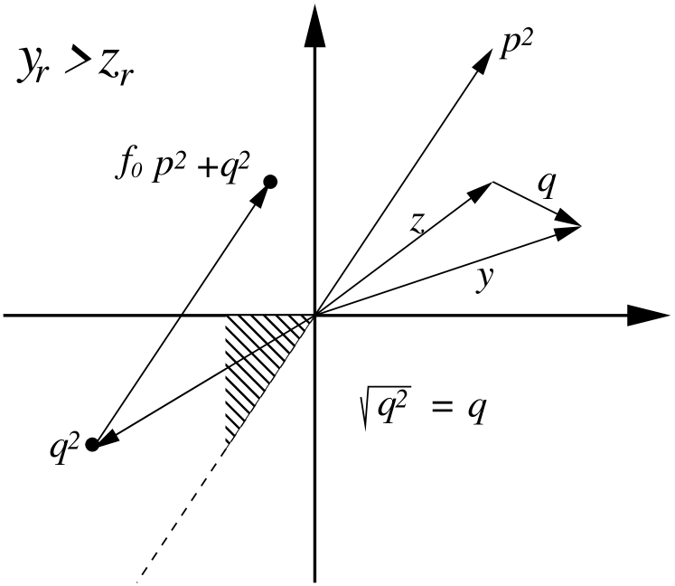
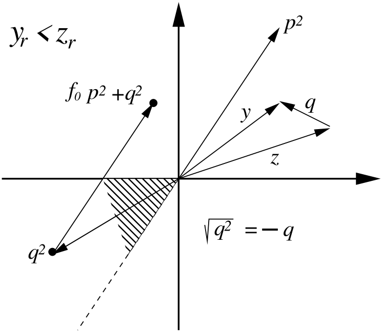
Figure 15: Diagram used in the classification of the eigenvalues of NDFW and FLL. Note that $y_{r}>z_{r}$ ( $y_{r}<z_{r}$) implies: $q_{r}>0$ ($q_{r}<0$), $\sqrt{q^{2}}=q$ ($\sqrt{q^{2}}=-q$).
The inequality $\{q_{2r}<0\,,q_{2i}<0\,,\frac{q_{2i}}{q_{2r}}<\frac{p_{2i}}{p_{2r}}\}$ is represented by the shaded areas in the figure and $f_{0}>-\frac{q_{2r}}{p_{2r}}$ implies ${\rm Re}\,(f_{0}p^{2}+q^{2})>0$.

The two eigenfrequencies coincide, $x_{dw}=x_{\ell a}$, when $\Delta=0$, what happens for $(y,z,f_{0})$ in the set

$$\bigg{\{}|z|=|y|\,,f_{0}=\tan^{2}(\psi/2)\bigg{\}}\,,$$ (C.217)

where $\psi$ is the angle between $y$ and $z$, $y={\rm e}^{i\psi}z$.

The NDFW and the FLL eigenfrequencies (this property does not extend to the eigenvectors) are dual to each other in the sense that if two bodies have the same $f_{0}$ but one has $(y,z)=(a_{1},a_{2})$ while the second $(y,z)=(a_{2},a_{1})$, then the value of $x_{dw}$ ($x_{\ell a}$) of the first is equal to the value of $x_{\ell a}$ ($x_{dw}$) of the second. This is a consequence of the symmetry of equation (6.128) with respect to the permutation of $y$ and $z$.

In the limit as the mantle becomes negligible, i.e. $f_{0}=\frac{{\rm I}_{\circ c}}{{\rm I}_{\circ m}}\to\infty$, we find two solutions to equation (6.128)

$$x_{c}=\frac{yz}{y+z}$$ (C.218)

and $(1+f_{0})(y+z)$. These solutions represent the limit of $x_{dw}(f_{0})$ and $x_{\ell a}(f_{0})$ as $f_{0}\to\infty$. In order to decide whether $x_{dw}$ or $x_{\ell a}$ is asymptotic to $x_{c}$, we solve equation (6.128) with $y=0$, the solutions being $x_{dw}(f_{0})=0=x_{c}$ and $x_{\ell a}(f_{0})=(f_{0}+1)z$, and with $z=0$, the solutions being $x_{\ell a}(f_{0})=0=x_{c}$ and $x_{dw}(f_{0})=(f_{0}+1)y$. Since $\Delta\neq 0$, by continuity the same result hold for $|y|$ small in the first case and $|z|$ small in the second. This fact, the duality of $x_{dw}$ and $x_{\ell a}$ discussed in the previous paragraph, and the invariance of $x_{c}$ and $(1+f_{0})(y+z)$ with respect to the permutation $y\leftrightarrow z$, lead us to:

$$\begin{split}&|y|<|z|\Longrightarrow x_{dw}(f_{0})\to x_{c}\ \ \text{and}\ \ x_{\ell a}(f_{0})\to(f_{0}+1)z\ \ \text{as}\ \ f_{0}\to\infty\\ &|z|<|y|\Longrightarrow x_{dw}(f_{0})\to(f_{0}+1)z\ \ \text{and}\ \ x_{\ell a}(f_{0})\to x_{c}\ \ \text{as}\ \ f_{0}\to\infty\,.\end{split}$$ (C.219)

Appendix D The Poincaré-Hough flow.

Following Poincaré (see Lamb (1932) paragraphs 146 and 384), let $\mathbf{x}_{0}\in\kappa$ be the position at time $t=0$ of a fluid particle inside a triaxial ellipsoid with semi-axes $A_{1}>A_{2}>A_{3}$. The mean radius of the ellipsoid is $R_{c}=(A_{1}A_{2}A_{3})^{1/3}$. For any time the center of the ellipsoid coincides with the origin of $\kappa$ and at $t=0$ the axes of the ellipsoid are aligned with the axes of $\kappa$. At $t=0$ the operator $\mathbf{A}:=$Diagonal$\{A_{1},A_{2},A_{3}\}$ maps the ball of radius one onto the ellipsoid. The ellipsoid is fixed in the frame of the mantle $\mathrm{K}_{m}$ and rotates inside the inertial frame $\kappa$ according to $\mathbf{R}_{m}(t):\mathrm{K}_{m}\to\kappa$, with $\mathbf{R}_{m}(0)=\mathbb{I}$. The motion of the fluid particle initially at $\mathbf{x}_{0}$ is assumed to be:

$$\mathbf{x}(t)=\mathbf{R}_{m}(t)\mathbf{A}\mathbf{R}_{f}(t)\mathbf{A}^{-1}\mathbf{x}_{0}\,,$$ (D.220)

where $t\to\mathbf{R}_{m}(t)$ is known. The unknown rotation matrix $\mathbf{R}_{f}(t)$ must be determined from the fluid dynamic equations.

The velocity field associated with the motion in equation (D.220) is

$$\mathbf{v}(\mathbf{x},t)=\dot{\mathbf{x}}=\underbrace{\big{(}\boldsymbol{\widehat{\omega}}_{m}+\mathbf{R}_{m}\mathbf{A}\boldsymbol{\widehat{\omega}}_{f}\mathbf{A}^{-1}\mathbf{R}_{m}^{-1}\big{)}}_{:=\mathbf{P}}\mathbf{x}=\mathbf{P}\mathbf{x}$$ (D.221)

It is convenient to split the operator $\mathbf{A}\boldsymbol{\widehat{\omega}}_{f}\mathbf{A}^{-1}$ into symmetric and anti-symmetric parts

$$\mathbf{A}\boldsymbol{\widehat{\omega}}_{f}\mathbf{A}^{-1}=\underbrace{\frac{1}{2}\Big{(}\mathbf{A}\boldsymbol{\widehat{\omega}}_{f}\mathbf{A}^{-1}+\big{(}\mathbf{A}\boldsymbol{\widehat{\omega}}_{f}\mathbf{A}^{-1}\big{)}^{T}\Big{)}}_{:=\mathbf{S}_{A}}+\underbrace{\frac{1}{2}\Big{(}\mathbf{A}\boldsymbol{\widehat{\omega}}_{f}\mathbf{A}^{-1}-\big{(}\mathbf{A}\boldsymbol{\widehat{\omega}}_{f}\mathbf{A}^{-1}\big{)}^{T}\Big{)}}_{:=\boldsymbol{\widehat{\tau}}}\,,$$ (D.222)

such that

$$\mathbf{P}=\boldsymbol{\widehat{\omega}}_{m}+\mathbf{R}_{m}\boldsymbol{\widehat{\tau}}\mathbf{R}_{m}^{-1}+\mathbf{R}_{m}\mathbf{S}_{A}\mathbf{R}_{m}^{-1}\,.$$ (D.223)

The expressions for $\mathbf{S}_{A}$ and $\boldsymbol{\tau}$ are

$$\mathbf{S}_{A}=\frac{1}{2}\left(\begin{array}[]{ccc}0&\left(\frac{A_{2}}{A_{1}}-\frac{A_{1}}{A_{2}}\right)\omega_{f3}&\left(\frac{A_{1}}{A_{3}}-\frac{A_{3}}{A_{1}}\right)\omega_{f2}\\ \left(\frac{A_{2}}{A_{1}}-\frac{A_{1}}{A_{2}}\right)\omega_{f3}&0&\left(\frac{A_{3}}{A_{2}}-\frac{A_{2}}{A_{3}}\right)\omega_{f1}\\ \left(\frac{A_{1}}{A_{3}}-\frac{A_{3}}{A_{1}}\right)\omega_{f2}&\left(\frac{A_{3}}{A_{2}}-\frac{A_{2}}{A_{3}}\right)\omega_{f1}&0\\ \end{array}\right)$$ (D.224)

and

$$\boldsymbol{\widehat{\tau}}=\frac{1}{2}\left(\begin{array}[]{ccc}0&-\left(\frac{A_{2}}{A_{1}}+\frac{A_{1}}{A_{2}}\right)\omega_{f3}&\left(\frac{A_{1}}{A_{3}}+\frac{A_{3}}{A_{1}}\right)\omega_{f2}\\ \left(\frac{A_{2}}{A_{1}}+\frac{A_{1}}{A_{2}}\right)\omega_{f3}&0&-\left(\frac{A_{3}}{A_{2}}+\frac{A_{2}}{A_{3}}\right)\omega_{f1}\\ -\left(\frac{A_{1}}{A_{3}}+\frac{A_{3}}{A_{1}}\right)\omega_{f2}&\left(\frac{A_{3}}{A_{2}}+\frac{A_{2}}{A_{3}}\right)\omega_{f1}&0\\ \end{array}\right)$$ (D.225)

Using that $\mathbf{v}=\mathbf{P}x=\boldsymbol{\omega}_{m}\times\mathbf{x}+(\mathbf{R}_{m}\boldsymbol{\tau})\times\mathbf{x}+\mathbf{R}_{m}\mathbf{S}_{A}\mathbf{R}_{m}^{-1}\mathbf{x}$ we obtain the vorticity field

$$\mathbf{w}:=\mathbf{curl}\,\mathbf{v}=2\big{(}\boldsymbol{\omega}_{m}+\mathbf{R}_{m}\boldsymbol{\tau}\big{)}\,,$$ (D.226)

which implies

$$\mathbf{P}=\frac{\mathbf{\widehat{w}}}{2}+\mathbf{R}_{m}\mathbf{S}_{A}\mathbf{R}_{m}^{-1}\quad\text{and}\quad\mathbf{v}=\frac{\mathbf{w}}{2}\times\mathbf{x}+\mathbf{R}_{m}\mathbf{S}_{A}\mathbf{R}_{m}^{-1}\mathbf{x}\,.$$ (D.227)

The equations for the motion of an inviscid, volume preserving, isentropic fluid are (Euler):

$$\begin{array}[]{lll}&\partial_{t}\mathbf{v}+\mathbf{v}\cdot\nabla\mathbf{v}=-\nabla h-\nabla\Phi&(\text{dynamical equation})\,,\\ &\mathbf{div}\,\mathbf{v}=0&(\text{incompressibility})\,,\\ &\partial_{t}\rho+\mathbf{div}\,(\rho\mathbf{v})=0&(\text{conservation of mass})\,,\end{array}$$ (D.228)

where: $\rho$ is the density, $h$ is the enthalpy ($dh=\frac{dp}{\rho}$ where $p$ is the pressure), and $\Phi$ is the external gravitational potential.

The divergence of $\mathbf{v}=\mathbf{P}x$ is zero because $\operatorname{Tr}(\mathbf{P})=0$. In order to fulfil the equation of continuity we impose that,

$$\rho(\mathbf{x},t)=\rho_{\circ}(r)\,,\ \ \text{where}\ \ r=\|\mathbf{A}^{-1}\mathbf{R}_{m}^{-1}(t)\mathbf{x}\|\,,0\leq r\leq R_{c}$$ (D.229)

If the fluid cavity would be slowly deformed to a round shape, then the density of the fluid inside the round core would be the radial function $\rho_{\circ}(r)$. Using that $\mathbf{div}\,\mathbf{v}=0$ the equation for conservation of mass can be written as $\partial_{t}\rho+\mathbf{v}\cdot\nabla\rho=\frac{d}{dt}\rho(\mathbf{x}(t),t)=0$. Equation (D.220) implies $\rho(\mathbf{x}(t),t)=\rho_{\circ}(\|\mathbf{A}^{-1}\mathbf{R}_{m}^{-1}(t)\mathbf{x}(t)\|)=\rho_{\circ}(\|\mathbf{A}^{-1}\mathbf{x}_{0}\|)$, so $\frac{d}{dt}\rho(\mathbf{x}(t),t)=0$ and the equation for conservation of mass is verified.

The last equation in (D.228) to be verified is the dynamical one. If we take the curl of this equation, then we obtain $\partial_{t}\mathbf{w}+\mathbf{v}\cdot\nabla\mathbf{w}-\mathbf{w}\cdot\nabla\mathbf{v}=0$, which is the dynamical equation for the vorticity. If the equation for the vorticity is verified, then the enthalpy can be determined integrating the dynamical equation for $\mathbf{v}$. Since $\mathbf{w}$ does not depend on $\mathbf{x}$, $\mathbf{v}\cdot\nabla\mathbf{w}=0$ and, since $\mathbf{v}=\mathbf{P}x$ depends linearly on $\mathbf{x}$, $\mathbf{w}\cdot\nabla\mathbf{v}=\mathbf{P}\mathbf{w}$, so the equation for the vorticity reduces to

$$\dot{\mathbf{w}}=\mathbf{P}\mathbf{w}\,.$$ (D.230)

This equation yields a simple ordinary differential equation for the unknown function $\boldsymbol{\omega}_{f}$ from which we determine the Poincaré-Hough flow.

Equation (D.227) implies that the Tisserand angular velocity $\boldsymbol{\omega}_{c}$ associated with the Poincaré-Hough flow satisfies

$$\boldsymbol{\pi}_{c}=\mathbf{I}_{c}\boldsymbol{\omega}_{c}=\int_{\mathcal{B}(t)}\rho(\mathbf{x}\times\mathbf{v})dx^{3}=\mathbf{I}_{c}\frac{\mathbf{w}}{2}+\int_{\mathcal{B}(t)}\rho\,\mathbf{x}\times\big{(}\mathbf{R}_{m}\mathbf{S}_{A}\mathbf{R}_{m}^{-1}\mathbf{x})dx^{3}$$ (D.231)

where $\mathcal{B}(t)$ is the set of points inside the cavity at time $t$. Since the density function is carried by the flow, $\mathbf{I}_{c}(t)=\mathbf{R}_{m}(t)\mathbf{I}_{c}(0)\mathbf{R}_{m}^{-1}(t)$.

In order to compute the moment of inertia of the fluid at $t=0$ we first compute the components of the density tensor $\mathbf{M}(0)$

$$M_{ij}(0)=\int_{\|\mathbf{A}^{-1}\mathbf{x}\|\leq 1}x_{i}x_{j}\rho_{\circ}(\|\mathbf{A}^{-1}\mathbf{x}\|)dx^{3}=\frac{A_{i}A_{j}}{R_{c}^{2}}\int_{\|\mathbf{y}\|\leq R_{c}}y_{i}y_{j}\rho_{\circ}(\|\mathbf{y}\|)dx^{3}\,,$$ (D.232)

where we did the change of variables $x_{i}=(A_{i}/R_{c})y_{i}$, $i=1,2,3$. Parity arguments imply that $M_{ij}(0)=0$ if $i\neq j$. Now, consider a round cavity of radius $R_{c}$ filled with a fluid with spherical density $\rho_{\circ}(r)$. The moment of inertia about any axis, say $\mathbf{e}_{3}$, of the spherical mass of fluid is

$${\rm I}_{\circ c}=\int_{\|\mathbf{y}\|\leq R_{c}}(y_{1}^{2}+y_{2}^{2})\rho_{\circ}(\|\mathbf{y}\|)dx^{3}$$ (D.233)

So, by symmetry $\int_{\|\mathbf{y}\|\leq R_{c}}y_{i}^{2}\rho_{\circ}(\|\mathbf{y}\|)dx^{3}={\rm I}_{\circ c}/2$ for any $i=1,2,3$ and

$$M_{ii}(0)=\frac{A_{i}^{2}}{R_{c}^{2}}\frac{{\rm I}_{\circ c}}{2}\,,\quad i=1,2,3\,.$$ (D.234)

Using that $\mathbf{I}_{c}=\operatorname{Tr}\big{(}\mathbf{M}\big{)}\mathbb{I}-\mathbf{M}$ we obtain

$$\mathbf{I}_{c}(0)=\frac{{\rm I}_{\circ c}}{2R_{c}^{2}}\left(\begin{array}[]{ccc}A_{2}^{2}+A_{3}^{2}&0&0\\ 0&A_{1}^{2}+A_{3}^{2}&0\\ 0&0&A_{1}^{2}+A_{2}^{2}\end{array}\right)$$ (D.235)

Note that $\operatorname{Tr}\mathbf{I}_{c}(0)={\rm I}_{\circ c}\frac{A_{1}^{2}+A_{2}^{2}+A_{3}^{2}}{R_{c}^{2}}$, so, ${\rm I}_{\circ c}$ may not have the usual meaning $\frac{1}{3}\operatorname{Tr}\mathbf{I}_{c}(0)$.

In order to compare the results obtained from the Poincaré-Hough flow with ours we have to assume that the fluid cavity is slightly aspherical, namely

$$A_{1}=R_{c}(1+\epsilon_{1})\quad A_{2}=R_{c}(1+\epsilon_{2})\quad A_{3}=R_{c}(1+\epsilon_{3})\,,$$ (D.236)

where $|\epsilon_{1}|,|\epsilon_{2}|,$ and $|\epsilon_{3}|$ are small. Since $A_{1}A_{2}A_{3}=R_{c}^{3}$, $\epsilon_{1}+\epsilon_{2}+\epsilon_{3}=0$ and equation (D.235) implies

$$\mathbf{I}_{c}(0)={\rm I}_{\circ c}\mathbb{I}+{\rm I}_{\circ c}\left(\begin{array}[]{ccc}\epsilon_{2}+\epsilon_{3}&0&0\\ 0&\epsilon_{1}+\epsilon_{3}&0\\ 0&0&\epsilon_{1}+\epsilon_{2}\end{array}\right)+\mathcal{O}(|\epsilon|^{2})\,,$$ (D.237)

so, $\frac{1}{3}\operatorname{Tr}\mathbf{I}_{c}(0)={\rm I}_{\circ c}$ holds up to second order in the ellipticity. Equation (D.224) implies

$$\mathbf{S}_{A}=\left(\begin{array}[]{ccc}0&\left(\epsilon_{2}-\epsilon_{1}\right)\omega_{f3}&\left(\epsilon_{1}-\epsilon_{3}\right)\omega_{f2}\\ \left(\epsilon_{2}-\epsilon_{1}\right)\omega_{f3}&0&\left(\epsilon_{3}-\epsilon_{2}\right)\omega_{f1}\\ \left(\epsilon_{1}-\epsilon_{3}\right)\omega_{f2}&\left(\epsilon_{3}-\epsilon_{2}\right)\omega_{f1}&0\\ \end{array}\right)+\mathcal{O}(|\epsilon|^{3})\,,$$ (D.238)

and equation (D.225) implies $\boldsymbol{\tau}=\boldsymbol{\omega}_{f}+\mathcal{O}(|\epsilon|^{2})$.

A computation shows that the last term in the right-hand side of equation (D.231) is of the order $\mathcal{O}(|\epsilon|^{2})$ and, therefore

$$\boldsymbol{\pi}_{c}=\mathbf{I}_{c}\boldsymbol{\omega}_{c}=\mathbf{I}_{c}\frac{\mathbf{w}}{2}+\mathcal{O}(|\epsilon|^{2})\Longrightarrow\boldsymbol{\omega}_{c}=\frac{\mathbf{w}}{2}+\mathcal{O}(|\epsilon|^{2})=\boldsymbol{\omega}_{m}+\mathbf{R}_{m}\boldsymbol{\omega}_{f}+\mathcal{O}(|\epsilon|^{2})$$ (D.239)

The fact that $\boldsymbol{\omega}_{c}\approx\mathbf{w}/2$ for small ellipticities has been noted in Henrard (2008).

For small ellipticities we can write $\boldsymbol{\omega}_{c}=\mathbf{w}/2$ and equation (D.230) implies

$$\dot{\boldsymbol{\omega}}_{c}=\mathbf{P}\boldsymbol{\omega}_{c}\,.$$ (D.240)

Therefore

$$\dot{\boldsymbol{\pi}}_{c}=\dot{\mathbf{I}}_{c}\boldsymbol{\omega}_{c}+{\mathbf{I}}_{c}\dot{\boldsymbol{\omega}}_{c}=\boldsymbol{\omega}_{m}\times\mathbf{I}_{c}\boldsymbol{\omega}_{c}+\mathbf{I}_{c}(-\boldsymbol{\widehat{\omega}}_{m}+\mathbf{P})\boldsymbol{\omega}_{c}$$ (D.241)

Equation (D.221) implies that the last term in the right-hand side of this equation can be written as

$$\mathbf{I}_{c}(-\boldsymbol{\widehat{\omega}}_{m}+\mathbf{P})\boldsymbol{\omega}_{c}=\mathbf{R}_{m}\mathbf{I}_{c}(0)\mathbf{A}\boldsymbol{\widehat{\omega}}_{f}\mathbf{A}^{-1}\mathbf{R}_{m}^{-1}\boldsymbol{\omega}_{c}\,.$$

A computation using equation (D.237) shows that $\mathbf{I}_{c}(0)\mathbf{A}\boldsymbol{\widehat{\omega}}_{f}\mathbf{A}^{-1}=\boldsymbol{\widehat{\omega}}_{f}\mathbf{I}_{c}(0)+\mathcal{O}(|\epsilon|^{2})$, so up to second order in the ellipticities

$$\dot{\boldsymbol{\pi}}_{c}=\boldsymbol{\omega}_{m}\times\mathbf{I}_{c}\boldsymbol{\omega}_{c}+\mathbf{R}_{m}\boldsymbol{\widehat{\omega}}_{f}\mathbf{I}_{c}(0)\mathbf{R}_{m}^{-1}\boldsymbol{\omega}_{c}=\boldsymbol{\omega}_{m}\times\mathbf{I}_{c}\boldsymbol{\omega}_{c}+\mathbf{R}_{m}\boldsymbol{\widehat{\omega}}_{f}\mathbf{R}_{m}^{-1}\mathbf{I}_{c}\boldsymbol{\omega}_{c}$$

and using equation (D.239) we obtain

$$\dot{\boldsymbol{\pi}}_{c}=\boldsymbol{\omega}_{c}\times\mathbf{I}_{c}\boldsymbol{\omega}_{c}$$ (D.242)

that is exactly the equation for the angular momentum of the core obtained in (5.77) with $k_{c}=0$.

We remark that the hypotheses we used in this Appendix to obtain the general results in equation (5.77) from the Poincaré-Hough flow, namely: small asphericity, density stratification along concentric ellipsoidal shells and the volume preserving property of the fluid flow; are the same hypotheses we have assumed since Ragazzo and Ruiz (2017). In this Appendix any rotational motion $\mathbf{R}_{m}(t)$ of the ellipsoid is allowed and there is no reason to assume that the principal axes of the mantle are aligned with those of the fluid cavity (a hypothesis commonly assumed). Finally, it is crucial for the results in this Appendix that the centre of mass of the mantle coincides with that of the fluid core for all time.

Appendix E The inertial offset of the core rotation axis.

In this appendix we analyse the effect of the inertial torque studied in Section 7 upon the fluid core. Two different situations will be considered: one without spin-orbit resonance and another with spin-orbit resonance.

E.1 Precession under no spin-orbit resonance, the Tisserand angular velocity of the fluid core, and the vorticity of Robert and Stewartson.

In this Section we assume that both the mantle and the core are axisymetric with $\overline{\gamma}=0$, $\overline{\alpha}=\overline{\beta}=\overline{\alpha}_{e}$, and $I_{c1}=I_{c2}=I_{c3}(1-f_{c})$, the mantle is rigid, and the precession rate is retrograde, $\dot{\psi}_{g}<0$. In this Section we further assume that $\eta_{c}/(\omega f_{c})\ll 1$. The goal is to study the angular velocity of the core produced exclusively by the inertial torque. The axisymmetry of the problem implies that in the precessional frame (equation (7.144)) both $\boldsymbol{\omega}_{m,pr}$ and $\boldsymbol{\omega}_{c,pr}$ are stationary, and according to equations (7.156) and (7.159) are given by

$$\begin{split}\boldsymbol{\omega}_{m,pr}&=\omega\mathbf{e}_{3}+\dot{\psi}_{g}\sin\theta_{g}\mathbf{e}_{2}+\omega\,\boldsymbol{\delta}_{m}\\ \boldsymbol{\omega}_{c,pr}&=\underbrace{\omega\mathbf{e}_{3}+\dot{\psi}_{g}\sin\theta_{g}\mathbf{e}_{2}}_{\boldsymbol{\omega}_{g,pr}}+\omega\,\boldsymbol{\delta}_{c}\end{split}$$ (E.243)

In order to write $\boldsymbol{\delta}_{c}$ we follow the same steps we did to obtain $\boldsymbol{\delta}_{m}$ in equation (7.164). After doing this and using that the complex compliance is null (the mantle is rigid) and $\eta_{c}/(\omega f_{c})\ll 1$ ($\Rightarrow y\approx f_{c}$ in equation (7.164)) we obtain

$$\begin{split}\boldsymbol{\delta}_{m}&=\frac{{\rm I_{\circ c}}}{{\,\rm I}_{\circ}}\frac{\dot{\psi}_{g}}{\omega f_{c}}\frac{2\cos^{2}\theta_{g}}{\sin\theta_{g}}\left(\frac{{\rm I}_{\circ m}}{{\,\rm I}_{\circ}}\frac{\eta_{c}}{f_{c}\,\omega}\,\mathbf{e}_{1}-\mathbf{e}_{2}\right)\\ \boldsymbol{\delta}_{c}&=\frac{\dot{\psi}_{g}}{\omega f_{c}}\sin\theta_{g}\left(1-2\frac{{\rm I}_{\circ c}}{{\,\rm I}_{\circ}}\cot^{2}\theta_{g}\right)\left(\mathbf{e}_{2}-\frac{{\rm I}_{\circ m}}{{\,\rm I}_{\circ}}\frac{\eta_{c}}{f_{c}\,\omega}\mathbf{e}_{1}\right)\\ &=\boldsymbol{\delta}_{m}+\frac{\dot{\psi}_{g}\,\sin\theta_{g}}{\omega f_{c}}\left(\mathbf{e}_{2}-\frac{{\rm I}_{\circ m}}{{\,\rm I}_{\circ}}\frac{\eta_{c}}{f_{c}\,\omega}\mathbf{e}_{1}\right)\end{split}$$ (E.244)

Roberts and Stewartson studied the motion of an incompressible fluid of constant density inside an ellipsoidal shell of revolution that precesses in the same way as the guiding motion used to obtain the angular velocities in equations (E.243) and (E.244). In Stewartson and Roberts (1963) and Roberts and Stewartson (1965) the authors solved the Navier-Stokes equations by perturbation methods (for a numerical study in the case of a spherical shell, see Tilgner and Busse (2001)) assuming the two hypotheses

$$\frac{f_{c}\,\omega}{|\dot{\psi}_{g}|}\gg 1\quad\text{ and}\quad f_{c}\,\omega\frac{R_{c}^{2}}{\nu}=f_{c}\,\frac{\omega}{\eta_{c}}\gg 1\,,$$ (E.245)

where: $R_{c}$ is the core mean radius, $\nu$ is kinematic viscosity of the fluid, and $\eta_{c}=R_{c}^{2}/\nu$ is the viscosity coefficient defined in equation (3.47). These are the same hypotheses we assumed to obtain equation (E.244). In the following we show that the difference $\boldsymbol{\omega}_{c,pr}-\boldsymbol{\omega}_{m,pr}=\omega(\boldsymbol{\delta}_{c}-\boldsymbol{\delta}_{m})$ is equal to the average vorticity of the flow inside the cavity, computed by Robert and Stewartson, minus the vorticity of the flow induced by a rigid rotation.

The velocity field of the fluid inside the cavity with respect to the precessional frame $\mathrm{K}_{pr}$ is Stewartson and Roberts (1963)

$$\mathbf{u}=\dot{\phi}_{g}\mathbf{e}_{3}\times\mathbf{x}+2\dot{\psi}_{g}\sin\theta_{g}\frac{a^{2}}{a^{2}-b^{2}}\left(x_{3}\mathbf{e}_{1}-\frac{b^{2}}{a^{2}}x_{1}\mathbf{e}_{3}\right)$$ (E.246)

where $b<a$ are the semi-axis of the cavity. The vorticity associated with this velocity field is

$${\rm curl}\,\mathbf{u}=2\dot{\phi}\mathbf{e}_{3}+2\dot{\psi}_{g}\sin\theta_{g}\frac{a^{2}+b^{2}}{a^{2}-b^{2}}\mathbf{e}_{2}$$ (E.247)

If the fluid were moving as a rigid body attached to the mantle, then its vorticity would be ${\rm curl}\dot{\phi}_{g}\mathbf{e}_{3}\times\mathbf{x}=2\dot{\phi}\mathbf{e}_{3}$. Recalling that vorticity is a measure of rotation of the vector field, as we have already mentioned in Appendix D,

$$2\dot{\psi}_{g}\sin\theta_{g}\frac{a^{2}+b^{2}}{a^{2}-b^{2}}\mathbf{e}_{2}=\underbrace{{\rm curl}\,\mathbf{u}}_{rot.fluid}-\underbrace{2\dot{\phi}\mathbf{e}_{3}}_{rot.mantle}$$ (E.248)

In order to relate equation (E.248) to the difference $\boldsymbol{\omega}_{c,pr}-\boldsymbol{\omega}_{m,pr}$ we use that the moments of inertia of an ellipsoid of revolution of constant density $\rho$ are $\overline{I}_{ce}=\frac{4\pi}{15}\rho(a^{2}+b^{2})a^{2}b$ and $\overline{I}_{c3}=\frac{8\pi}{15}\rho a^{4}b$ that implies

$$f_{c}=\frac{\overline{I}_{c3}-\overline{I}_{ce}}{\overline{I}_{c3}}\approx\frac{\overline{I}_{3}-\overline{I}_{ce}}{\overline{I}_{ce}}=\frac{a^{2}-b^{2}}{a^{2}+b^{2}}$$ (E.249)

Therefore, using the second hypothesis of Robert and Stewartson $\frac{\eta_{c}}{f_{c}\omega}\ll 1$ (equation (E.245)) equations (E.243), (E.244), (E.248), and (E.249) imply the claimed result:

$$\boldsymbol{\omega}_{c,pr}-\boldsymbol{\omega}_{m,pr}\approx\frac{1}{2}\bigg{(}{\rm curl}\,\mathbf{u}-2\dot{\phi}\mathbf{e}_{3}\bigg{)}=\frac{\dot{\psi}_{g}}{f_{c}}\sin\theta_{g}\mathbf{e}_{2}\,.$$ (E.250)

We could also have computed the total angular momentum of the fluid with respect to the precessional frame and arrived at the same result.

E.2 The resonant case and the Cassini states of G. Boué.

The Cassini states of a body made of a rigid mantle and a fluid core with no viscous coupling ($k_{c}=\eta_{c}=0$) were computed in Boué (2020). In ibid, the difference between the angular velocities of mantle and core was not supposed small and many possible Cassini states were found. Our goal in the rest of this Appendix is to compare the inertial offsets $\boldsymbol{\delta}_{m}$ and $\boldsymbol{\delta}_{c}$ with some of the Cassini states found in Boué (2020).

The expressions for $\boldsymbol{\delta}_{m}$ and $\boldsymbol{\delta}_{c}$ in equations (7.166) simplify when we assume that: the moment of inertia of the fluid core is not much smaller than that of the mantle, the mantle is rigid, and $\eta_{c}=0$,

$$\begin{split}&\delta_{m}=\delta_{m2}=-\frac{\frac{{\rm I}_{\circ c}}{{\rm I}_{\circ m}}\frac{\dot{\psi}_{g}}{\omega}\cos\theta_{g}}{\left(\frac{\dot{\psi}_{g}}{\omega}\cos\theta_{g}\right)^{2}+\frac{\dot{\psi}_{g}}{\omega}\cos\theta_{g}\frac{{\,\rm I}_{\circ}}{{\rm I}_{\circ m}}(y+z)+\frac{{\,\rm I}_{\circ}}{{\rm I}_{\circ m}}yz}\frac{\dot{\psi}_{g}}{\omega}\sin\theta_{g}\,,\\ &\delta_{c}=\delta_{c2}=\frac{\frac{{\,\rm I}_{\circ}}{{\rm I}_{\circ m}}z+\frac{\dot{\psi}_{g}}{\omega}\cos\theta_{g}}{\left(\frac{\dot{\psi}_{g}}{\omega}\cos\theta_{g}\right)^{2}+\frac{\dot{\psi}_{g}}{\omega}\cos\theta_{g}\frac{{\,\rm I}_{\circ}}{{\rm I}_{\circ m}}(y+z)+\frac{{\,\rm I}_{\circ}}{{\rm I}_{\circ m}}yz}\frac{\dot{\psi}_{g}}{\omega}\sin\theta_{g}\,,\end{split}$$ (E.251)

where $z=c_{1}\overline{\alpha}_{e}+\frac{c_{2}}{2}\overline{\gamma}$ and $y=f_{c}$. According to equation (7.159) all the three vectors: the normal to the invariable plane $\mathbf{e}_{3}\in\kappa$, the angular velocity of the mantle $\langle\boldsymbol{\omega}_{m}\rangle_{pr}\in\kappa$, and the angular velocity of the core $\langle\boldsymbol{\omega}_{c}\rangle_{pr}\in\kappa$, both averaged in the precessional frame; are contained in the same plane, which is denoted by $\Sigma$ in Figure 8 LEFT.

The Cassini states in Boué (2020) are determined by the following two equations (Equations (34a) and (34b) in ibid.)

$$\begin{split}&f_{c}\dot{\phi}_{g}\cos(\delta_{m}-\delta_{c})\sin(\delta_{m}-\delta_{c})+\dot{\psi}_{g}\sin(\theta_{g}-\delta_{c})=0\\ &\overline{I}_{c3}\Big{(}\dot{\psi}_{g}\sin(\theta_{g}-\delta_{m})+f_{c}\dot{\phi}_{g}\cos(\delta_{m}-\delta_{c})\sin(\delta_{m}-\delta_{c})\Big{)}-\frac{\overline{I}_{3}\omega^{2}}{\dot{\phi}_{g}}P_{e}(\delta_{m})=0\end{split}$$ (E.252)

where

$$\begin{split}P_{e}(\delta_{m})=&\frac{3}{2}\frac{Gm_{p}}{a_{p}^{3}\omega^{2}}\bigg{(}\overline{\alpha}_{e}X^{-3,0}_{0}\cos(\chi_{p}-\delta_{m})\sin(\chi_{p}-\delta_{m})\\ &+\frac{\overline{\gamma}}{4}X^{-3,2}_{s}\big{(}1+\cos(\chi_{p}-\delta_{m})\big{)}\sin(\chi_{p}-\delta_{m})\bigg{)}+\frac{\dot{\psi}_{g}\dot{\phi}_{g}}{\omega^{2}}\sin(\theta_{g}-\delta_{m})\,.\end{split}$$ (E.253)

The identity $P_{e}(0)=0$ holds due to Peale’s equation (7.148).

Since our inertial offset was computed by means of a perturbation of a rigid-body motion, for which $\delta_{m}=\delta_{c}=0$, it is natural to look for solutions $(\delta_{m},\delta_{c})\approx(0,0)$ to equations (E.252). For $(\delta_{m},\delta_{c})=(0,0)$, the first equation in (E.252) implies $\dot{\psi}_{g}\sin(\theta_{g})=0$ and then the second equation implies

$$P_{e}(0)=0\Longrightarrow\bigg{(}\overline{\alpha}_{e}X^{-3,0}_{0}\cos(\chi_{p})+\frac{\overline{\gamma}}{4}X^{-3,2}_{s}\big{(}1+\cos(\chi_{p})\big{)}\bigg{)}\sin(\chi_{p})=0\,.$$ (E.254)

This equation has several solutions $\chi_{p}=0$, $\chi_{p}=\pi$, and $\cos\chi_{p}=-\frac{\overline{\gamma}X^{-3,2}_{s}}{4\overline{\alpha}_{e}X^{-3,0}_{0}+\overline{\gamma}X^{-3,2}_{s}}$, where $\chi_{p}$ is the obliquity of the body spin to the orbital plane. Among these solutions only $\chi_{p}=0$ has obliquity smaller then $\pi/2$ (except $\cos\chi_{p}=-\frac{\overline{\gamma}X^{-3,2}_{s}}{4\overline{\alpha}_{e}X^{-3,0}_{0}+\overline{\gamma}X^{-3,2}_{s}}$ with s=1, for which the obliquity is smaller but close to $\pi/2$). We will only consider solutions to equations (E.252) with obliquities smaller than $\pi/2$ that originate from $\chi_{p}=0$.

In order to show that the small solutions $(\delta_{m},\delta_{c})$ to equations (E.252) are given by equation (E.251), it is enough to expand the functions in the left-hand side of equations (E.252) up to first order in $(\delta_{m},\delta_{c})$ and then to solve the linear system. This was done using the algebraic manipulator Mathematica.

The Hessian determinant of equation (E.252) is proportional to $(x_{\ell a}+\frac{\dot{\psi}_{g}}{\omega}\cos\theta_{g})(x_{dw}+\frac{\dot{\psi}_{g}}{\omega}\cos\theta_{g})$, where $\omega x_{dw}$ and $\omega x_{\ell a}$ are the eigenfrequencies of the nearly diurnal free wobble (NDFW) and the free libration in latitude (FLL) in the inertial space. This shows that the critical flattening of the core $f_{c}\approx 0.005\overline{\alpha}_{c}$ found for Mercury in Section 6.1 of Boué (2020) (see also Figure 3 in ibid.) is indeed a resonance of the precession angular speed $-\dot{\psi}_{d}\cos\theta_{g}\approx$330 kyr with the NDFW eigenfrequency, which decreases to zero as $f_{c}\to 0$. The presence of dissipation attenuates the singularity, as illustrated in Figure 9.

References

- Arnold [1992] V.I. Arnold. Ordinary Differential Equations. Springer Textbook. Springer Berlin Heidelberg, 1992. ISBN 9783540548133.
- Baland et al. [2017] Rose-Marie Baland, Marie Yseboodt, Attilio Rivoldini, and Tim Van Hoolst. Obliquity of Mercury: Influence of the precession of the pericenter and of tides. Icarus, 291:136–159, 2017.
- Batchelor [2000] GK Batchelor. An introduction to fluid dynamics. Cambridge university press, 2000.
- Beuthe [2015] Mikael Beuthe. Tidal Love numbers of membrane worlds: Europa, Titan, and Co. Icarus, 258:239–266, 2015.
- Bland [1960] DR Bland. Linear viscoelasticity. Pergamon Press, Oxford, 1960.
- Boué [2020] Gwenaël Boué. Cassini states of a rigid body with a liquid core. Celestial Mechanics and Dynamical Astronomy, 132:1–26, 2020.
- Boué et al. [2017] Gwenaël Boué, Nicolas Rambaux, and Andy Richard. Rotation of a rigid satellite with a fluid component: a new light onto Titan’s obliquity. Celestial Mechanics and Dynamical Astronomy, 129(4):449–485, 2017.
- Běhounková et al. [2010] Marie Běhounková, Gabriel Tobie, Gaël Choblet, and Ondřej Čadek. Coupling mantle convection and tidal dissipation: Applications to Enceladus and Earth-like planets. Journal of Geophysical Research (Planets), 115(E9):E09011, September 2010. doi: 10.1029/2009JE003564.
- Běhounková et al. [2017] Marie Běhounková, Ondřej Souček, Jaroslav Hron, and Ondřej Čadek. Plume Activity and Tidal Deformation on Enceladus Influenced by Faults and Variable Ice Shell Thickness. Astrobiology, 17(9):941–954, September 2017. doi: 10.1089/ast.2016.1629.
- Capitaine et al. [1986] Nicole Capitaine, B Guinot, and J Souchay. A non-rotating origin on the instantaneous equator: definition, properties and use. Celestial mechanics, 39(3):283–307, 1986.
- Chandrasekhar [1969] Subrahmanyan Chandrasekhar. Ellipsoidal figures of equilibrium. Yale Univ. Press, 1969.
- Colombo [1966] G Colombo. Cassini’s second and third laws. The Astronomical Journal, 71:891, 1966.
- Correia et al. [2018] ACM Correia, C Ragazzo, and LS Ruiz. The effects of deformation inertia (kinetic energy) in the orbital and spin evolution of close-in bodies. Celestial Mechanics and Dynamical Astronomy, 130(8):51, 2018.
- Correia and Delisle [2019] Alexandre CM Correia and Jean-Baptiste Delisle. Spin-orbit coupling for close-in planets. Astronomy & Astrophysics, 630:A102, 2019.
- Correia et al. [2014] Alexandre CM Correia, Gwenaël Boué, Jacques Laskar, and Adrián Rodríguez. Deformation and tidal evolution of close-in planets and satellites using a Maxwell viscoelastic rheology. Astronomy & Astrophysics, 571:A50, 2014.
- Deleplace and Cardin [2006] Bérangère Deleplace and Philippe Cardin. Viscomagnetic torque at the core mantle boundary. Geophysical Journal International, 167(2):557–566, 2006.
- Eckhardt [1981] Donald H Eckhardt. Theory of the libration of the Moon. The Moon and the planets, 25(1):3–49, 1981.
- Efroimsky [2012a] Michael Efroimsky. Bodily tides near spin–orbit resonances. Celestial Mechanics and Dynamical Astronomy, 112(3):283–330, 2012a.
- Efroimsky [2012b] Michael Efroimsky. Tidal dissipation compared to seismic dissipation: In small bodies, Earths, and super-Earths. The Astrophysical Journal, 746(2):150, 2012b.
- Ferraz-Mello et al. [2020] Sylvio Ferraz-Mello, Cristian Beaugé, Hugo A Folonier, and Gabriel O Gomes. Tidal friction in satellites and planets. the new version of the creep tide theory. The European Physical Journal Special Topics, 229:1441–1462, 2020.
- Fienga et al. [2019] A. Fienga, P. Deram, V. Viswanathan, A. Di Ruscio, L. Bernus, D. Durante, M. Gastineau, and J. Laskar. INPOP19a planetary ephemerides. Notes Scientifiques et Techniques de l’Institut de Mécanique Céleste, 109, December 2019.
- Folkner et al. [2014] W. M. Folkner, J. G. Williams, D. H. Boggs, R. S. Park, and P. Kuchynka. The Planetary and Lunar Ephemerides DE430 and DE431. Interplanetary Network Progress Report, 42-196:1–81, Feb 2014.
- Folonier and Ferraz-Mello [2017] Hugo A. Folonier and Sylvio Ferraz-Mello. Tidal synchronization of an anelastic multi-layered body: Titan’s synchronous rotation. Celestial Mechanics and Dynamical Astronomy, 129(4):359–396, December 2017. doi: 10.1007/s10569-017-9777-5.
- Genova et al. [2016] Antonio Genova, Sander Goossens, Frank G Lemoine, Erwan Mazarico, Gregory A Neumann, David E Smith, and Maria T Zuber. Seasonal and static gravity field of Mars from MGS, Mars Odyssey and MRO radio science. Icarus, 272:228–245, 2016.
- Gevorgyan [2021] Yeva Gevorgyan. Homogeneous model for the TRAPPIST-1e planet with an icy layer. Astronomy & Astrophysics, 650:A141, June 2021. doi: 10.1051/0004-6361/202140736.
- Gevorgyan et al. [2020] Yeva Gevorgyan, Gwenaël Boué, Clodoaldo Ragazzo, Lucas S. Ruiz, and Alexandre C.M. Correia. Andrade rheology in time-domain. application to Enceladus’ dissipation of energy due to forced libration. Icarus, 343:113610, 2020. ISSN 0019-1035. doi: https://doi.org/10.1016/j.icarus.2019.113610. URL http://www.sciencedirect.com/science/article/pii/S0019103519305020.
- Glickman [2000] Glickman. Glossary of Meteorology. American Meteorological Society, 2000. ISBN 9781878220349.
- Goldreich and Toomre [1969] Peter Goldreich and Alar Toomre. Some remarks on polar wandering. Journal of Geophysical Research, 74(10):2555–2567, 1969.
- Gross [2007] Richard S Gross. Earth rotation variations-long period. Treatise on geophysics, 3:239–294, 2007.
- Guinot [1979] Bernard Guinot. Basic problems in the kinematics of the rotation of the Earth. In Symposium-International Astronomical Union, volume 82, pages 7–18. Cambridge University Press, 1979.
- Henrard [2008] Jacques Henrard. The rotation of Io with a liquid core. Celestial Mechanics and Dynamical Astronomy, 101(1-2):1–12, 2008.
- Holm et al. [2009] D. D. Holm, T. Schmah, and C. Stoica. Geometric Mechanics and Symmetry. Oxford University Press, New York, 2009.
- Hough [1895] Sydney Samuel Hough. Xii. the oscillations of a rotating ellipsoidal shell containing fluid. Philosophical Transactions of the Royal Society of London.(A.), 186:469–506, 1895.
- Iess et al. [2014] Luciano Iess, DJ Stevenson, M Parisi, D Hemingway, RA Jacobson, JI Lunine, F Nimmo, JW Armstrong, SW Asmar, M Ducci, et al. The gravity field and interior structure of Enceladus. Science, 344(6179):78–80, 2014.
- Jacobson and Lainey [2014] RA Jacobson and V Lainey. Martian satellite orbits and ephemerides. Planetary and Space Science, 102:35–44, 2014.
- Lainey [2016] Valéry Lainey. Quantification of tidal parameters from Solar System data. Celestial Mechanics and Dynamical Astronomy, 126(1-3):145–156, 2016.
- Lamb [1932] H. Lamb. Hydrodynamics. Cambridge Mathematical Library, Cambridge, 6th edition, 1932.
- Lambeck [1980] K. Lambeck. The Earth’s variable rotation: geophysical causes and consequences. Cambridge University Press, UK, 1980.
- Margot et al. [2018] Jean-Luc Margot, SA Hauck II, E Mazarico, Stanton J Peale, and Sebastiano Padovan. Mercury’s internal structure. Mercury-The view after MESSENGER, pages 85–113, 2018.
- Mathews et al. [2002] Piravonu Mathews Mathews, Thomas A Herring, and Bruce Allen Buffett. Modeling of nutation and precession: New nutation series for nonrigid Earth and insights into the Earth’s interior. Journal of Geophysical Research: Solid Earth, 107(B4):ETG–3, 2002.
- Matsui and Buffett [2012] Hiroaki Matsui and Bruce A Buffett. Large-eddy simulations of convection-driven dynamos using a dynamic scale-similarity model. Geophysical & Astrophysical Fluid Dynamics, 106(3):250–276, 2012.
- Matsuyama [2014] Isamu Matsuyama. Tidal dissipation in the oceans of icy satellites. Icarus, 242:11–18, November 2014. doi: 10.1016/j.icarus.2014.07.005.
- Matsuyama et al. [2018] Isamu Matsuyama, Mikael Beuthe, Hamish C. F. C. Hay, Francis Nimmo, and Shunichi Kamata. Ocean tidal heating in icy satellites with solid shells. Icarus, 312:208–230, September 2018. doi: 10.1016/j.icarus.2018.04.013.
- Mazarico et al. [2014] Erwan Mazarico, Antonio Genova, Sander Goossens, Frank G Lemoine, Gregory A Neumann, Maria T Zuber, David E Smith, and Sean C Solomon. The gravity field, orientation, and ephemeris of Mercury from MESSENGER observations after three years in orbit. Journal of Geophysical Research: Planets, 119(12):2417–2436, 2014.
- McKenzie [1966] Dan P McKenzie. The viscosity of the lower mantle. Journal of Geophysical Research, 71(16):3995–4010, 1966.
- Munk and MacDonald [1961] W. H. Munk and G. J. F. MacDonald. The rotation of the Earth. Cambridge University Press, New York, 1961.
- Nastula and Gross [2015] J Nastula and R Gross. Chandler wobble parameters from SLR and GRACE. Journal of Geophysical Research: Solid Earth, 120(6):4474–4483, 2015.
- Nimmo and Pappalardo [2016] F. Nimmo and R. T. Pappalardo. Ocean worlds in the outer solar system. Journal of Geophysical Research (Planets), 121(8):1378–1399, August 2016. doi: 10.1002/2016JE005081.
- Noyelles [2018] Benoît Noyelles. Rotation of a synchronous viscoelastic shell. Monthly Notices of the Royal Astronomical Society, 474(4):5614–5644, 2018.
- Park et al. [2021] Ryan S. Park, William M. Folkner, James G. Williams, and Dale H. Boggs. The JPL Planetary and Lunar Ephemerides DE440 and DE441. The Astronomical Journal, 161(3):105, March 2021. doi: 10.3847/1538-3881/abd414.
- Peale [1969] Stanton J Peale. Generalized Cassini’s laws. The Astronomical Journal, 74:483, 1969.
- Peale [1974] Stanton J Peale. Possible histories of the obliquity of Mercury. The Astronomical Journal, 79:722, 1974.
- Peale et al. [2014] Stanton J. Peale, Jean-Luc Margot, Steven A. Hauck, and Sean C. Solomon. Effect of core-mantle and tidal torques on Mercury’s spin axis orientation. Icarus, 231:206–220, mar 2014. doi: 10.1016/j.icarus.2013.12.007.
- Pedlosky [2013] Joseph Pedlosky. Geophysical fluid dynamics. Springer Science & Business Media, 2013.
- Petit and Luzum [2010] Gérard Petit and Brian Luzum. IERS conventions (2010). Technical report, DTIC Document, 2010.
- Poincaré [1885] Henri Poincaré. Sur l’équilibre d’une masse fluide animée d’un mouvement de rotation. Acta mathematica, 7(1):259–380, 1885.
- Poincaré [1910] Henri Poincaré. Sur la précession des corps déformables. Bulletin Astronomique, Serie I, 27:321–356, 1910.
- Ragazzo and Ruiz [2017] C. Ragazzo and L. S. Ruiz. Viscoelastic tides: models for use in Celestial Mechanics. Celestial Mechanics and Dynamical Astronomy, 128(1):19–59, May 2017. doi: 10.1007/s10569-016-9741-9.
- Ragazzo and Ruiz [2015] C Ragazzo and LS Ruiz. Dynamics of an isolated, viscoelastic, self-gravitating body. Celestial Mechanics and Dynamical Astronomy, 122(4):303–332, 2015.
- Ragazzo [2020] Clodoaldo Ragazzo. The theory of figures of Clairaut with focus on the gravitational modulus: inequalities and an improvement in the Darwin–Radau equation. São Paulo Journal of Mathematical Sciences, 14:1–48, 2020.
- Ragazzo and Ruiz [2017] Clodoaldo Ragazzo and LS Ruiz. Viscoelastic tides: models for use in Celestial Mechanics. Celestial Mechanics and Dynamical Astronomy, 128(1):19–59, 2017.
- Rambaux and Williams [2011] N Rambaux and JG Williams. The Moon’s physical librations and determination of their free modes. Celestial Mechanics and Dynamical Astronomy, 109(1):85–100, 2011.