Computing and Maintaining Provenance of Query Result Probabilities in Uncertain Knowledge Graphs

Abstract.

Knowledge graphs (KG) that model the relationships between entities as labeled edges (or facts) in a graph are mostly constructed using a suite of automated extractors, thereby inherently leading to uncertainty in the extracted facts. Modeling the uncertainty as probabilistic confidence scores results in a probabilistic knowledge graph. Graph queries over such probabilistic KGs require answer computation along with the computation of those result probabilities, aka, probabilistic inference. We propose a system, HaPPI (How Provenance of Probabilistic Inference), to handle such query processing. Complying with the standard provenance semiring model, we propose a novel commutative semiring to symbolically compute the probability of the result of a query. These provenance-polynomial-like symbolic expressions encode fine-grained information about the probability computation process. We leverage this encoding to efficiently compute as well as maintain the probability of results as the underlying KG changes. Focusing on a popular class of conjunctive basic graph pattern queries on the KG, we compare the performance of HaPPI against a possible-world model of computation and a knowledge compilation tool over two large datasets. We also propose an adaptive system that leverages the strengths of both HaPPI and compilation based techniques. Since existing systems for probabilistic databases mostly focus on query computation, they default to re-computation when facts in the KG are updated. HaPPI, on the other hand, does not just perform probabilistic inference and maintain their provenance, but also provides a mechanism to incrementally maintain them as the KG changes. We extend this maintainability as part of our proposed adaptive system.

1. Introduction

Knowledge graphs (KGs) are central to many real-life systems such as search engines, social networks, medical assistants, question answering, etc. Some of these KGs are automatically built by employing a suite of knowledge extractors and integrators. Differences in various extraction approaches, inherent ambiguities of the extraction process itself, and variations in the credibility of data sources make the automatically extracted facts uncertain. The uncertainty is encoded by assigning a confidence score to each fact, leading to probabilistic knowledge graphs such as YAGO2 (Hoffart et al., 2013), NELL (Mitchell et al., 2015), ReVerb (Fader et al., 2011), Probase (Wu et al., 2012), etc.

In addition, despite the phenomenal progress in information extraction techniques, erroneous facts invariably creep into KGs. This, in turn, results in query answers being erroneous. For instance, the query for “a list of African comedians” over the NELL KG includes “Jimmy Fallon” and “Ellen DeGeneres” (as per NELL extraction round #1082). Although both are comedians, neither of them are from Africa. To determine the source of the error, or to debug the KG, it is necessary to compute the provenance of each result.

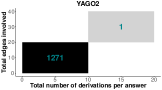
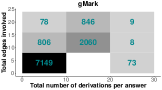
Figure 1. Distribution of YAGO2 and gMark query answers according to their total derivations and involved edges

Provenance represents the derivation process of an answer. For probabilistic data, typically, it is modeled as a Boolean formula in disjunctive normal form (DNF), where each conjunct encodes a derivation. This Boolean formula, referred to as lineage, is also used for probability computation of the answer by counting all satisfying assignments – equivalent to the model counting problem which is known to be #P-hard  (Roth, 1996). The brute-force way of counting satisfying assignments, known as possible world computation, is to iterate over all possible assignments taking time exponential in the number of the Boolean variables involved. For provenance in probabilistic graphs, a Boolean variable is associated with each edge. A more nuanced approach to probability computation is the knowledge compilation technique that translates the lineage formula to a more tractable Boolean circuit using SAT solvers. Although it cannot guarantee scalability, for large answers the use of compilation tools (e.g., C2D (Darwiche, 2004), D4 (Lagniez and Marquis, 2017), dSharp (Muise et al., 2012)) is known to be practical.

However, for answers with a small number of Boolean variables in their derivation formula, the overhead of a SAT solver invocation results in a considerably poor performance. Naïvely using knowledge compilation tools may, thus, fail to take advantage of small size of the computation problem. We investigated the results of query workloads from gMark (Bagan et al., 2017) as well as YAGO2 (Hoffart et al., 2013) to understand the extent to which this behavior can affect the overall performance. Fig. 1 summarizes the distribution of answers with different number of derivations (along x-axis) and edge counts (along y-axis), suitably bucketed for readability. We use color to indicate the absolute count of answers in each region (darker the color, more the count), and also print the raw count. It can be seen that most graph query answers are concentrated in the area where the derivation and edge counts are low—precisely where knowledge compilation is not the best method. In fact, in this region, they are out-performed by even a possible-world computation that employs brute-force evaluation.

In this paper, we specifically target this region where a large number of answers are found, and present an algorithm for probability computations that significantly speeds up the performance there. We implement this in a system named HaPPI (How Provenance of Probabilistic Inference). Thematically to the provenance semiring model (Green et al., 2007), we also introduce a novel semiring which enables HaPPI to symbolically compute the answer probability. The proposed semiring facilitates computing how provenance of not just the query answer but also of its probability computation. Unlike a Boolean formula that simply represents how edges interact to generate an answer, we additionally capture the arithmetic involved to compute the exact probability. This fine-grained provenance information allows for efficient maintenance in HaPPI.

HaPPI outperforms knowledge compilation tools as well as possible world computation for answers of the kind found in the highly populated bottom left region of Fig. 1. Since knowledge compilation techniques work best for answers with high derivation and edge counts, we also propose an adaptive system that uses HaPPI for small answers and compilation techniques for larger answers. We show that this adaptive system produces sizeable gains in performance over either system used in isolation. Further, since the adaptive system uses HaPPI for a large number of answers, it inherits the maintainability of HaPPI.

The key contributions of this paper are four-fold:

1. A novel theoretical model (Sec. 4) based on a semiring to support efficient probability computation over probabilistic KGs.

2. A practical implementation (Sec. 5), HaPPI , extends a provenance-aware property graph system, HUKA . Our algorithm can be also used in conjunction with other works, like HUKA (Gaur et al., 2020, 2017) and ProvSQL (Senellart et al., 2018), based on the same underlying system to expand their support for probabilistic data.

3. A theoretical analysis as well as an empirical evaluation highlighting the easy maintainability of HaPPI under insertion of edges (i.e., new facts) to the KG.

4. Finally, a proposal for an adaptive framework that leverages the superior performance of HaPPI and knowledge compilation tools at different regions of answer sizes. Our extensive empirical evaluation, using queries over gMark, a synthetic KG, and, YAGO2, a real-world KG, shows that this adaptive system outperforms any existing method used in isolation.

(a) Knowledge graph

(b) Query pattern

Figure 2. Running example of flight knowledge graph, a query for pairs of cities with one-stop connection between them, and a listing of edge probabilities.

2. Background

2.1. Probabilistic Knowledge Graph

A probabilistic knowledge graph is a graph $G\left(V,E,L,Id,Pr\right)$ with vertex-set $V$ representing the entities, labeled edge-set $E$ with each edge $e$ represented as $\langle u,l,v\rangle$ with $l\in L$ encoding the relation between two vertices $u$ and $v$. It is also common to refer to an edge $e=\langle u,l,v\rangle$ in the knowledge graph as a fact where $u$, $l$, $v$ are subject, predicate and object of the fact respectively. Each edge is assigned a unique id, ${Id}:E\to\mathcal{N}$. Further, we associate with each edge a value between $0$ and $1$, $Pr:E\to[0,1]$, representing the probability of the corresponding fact. We make the standard edge independence assumption where the existence of an edge is independent of the other edges in the KG. Unlike a deterministic KG, the presence of each fact in the KG is a probabilistic event, the probability of which is referred to as the existential probability of the fact.

Possible World Semantics

Equivalently, we can interpret the probabilistic knowledge graph as a collection of edge-induced subgraphs, called possible worlds, $\mathcal{G_{PW}}=\{G_{1},\dots,G_{n}\}$ of the knowledge graph $G$. There is a probability distribution, $\mathcal{P}$, defined over all possible worlds, such that $\Sigma_{G_{i}\in G_{PW}}\mathcal{P}(G_{i})=1.$ With edge-independence assumption as before, $P(G_{i})$ in terms of probability of its edges is

(1) $$\mathcal{P}(G_{i})=\prod_{e_{i}\in E_{i}}Pr(e_{i})\times\prod_{e_{i}\in E\setminus E_{i}}(1-Pr(e_{i}))$$

where $E_{i}$ is the set of edges present in $G_{i}$.

2.2. Graph Query

A graph query is formulated as a graph pattern that a user intends to find in the knowledge graph $G$. Similar to the triple representation of KG, a graph query expresses the query graph pattern as a collection of triples. Each edge of the graph pattern corresponds to a triple pattern in the query. Similar to graph triples, a triple pattern consists of subject, predicate, and object. Both subject and object can be variables or be bound to one of the vertices of the KG. A predicate could be a variable or one of the labels of the edges of the KG. A graph query pattern can be realized as a query using the SPARQL query language.

A graph query can be interpreted as a conjunction of triple patterns and the aim is to find all possible bindings to the variables of the triple patterns as a whole. These conjunctive graph queries are popularly known as Basic Graph Pattern (BGP) queries (Harris et al., 2013). Such SPARQL queries can be expressed as relational SPJ (Select-Project-Join) queries (Cyganiak, 2005). In this work we are handling a subset of SPARQL queries which does not include more sophisticated operators such as Union, Optional, etc. We see inclusion of these SPARQL queries as future work.

2.3. Running Example

Throughout the paper we use the following running example. Consider an air-travel agency that provides a flight search engine. The search engine uses the knowledge graph shown in Fig. 2(a) as its knowledge base. The nodes in the graph denote the airport codes of different cities it operates in: Singapore (SIN), New Delhi (DEL), Munich (MUN), Barcelona (BAR), and New York (JFK). An edge between two cities represents a direct flight with edge label representing the airline operating the flight. The operation of each flight is dependent on different factors, like environmental, financial, political, etc. Thus, the existence of the edges in the graph is a probabilistic event. Each edge of the KG, shown in Fig. 2(a), is annotated with its existential probability. Suppose a user wants to list down all the pairs of cities that have one-stop connecting flights between them with a joint probability greater than $0.5$. The corresponding query pattern, shown in Fig. 2(b), and the equivalent SPARQL query,

Select ?city1 ?city2 Where {
       ?city1 ?x1 ?city2.
       ?city2 ?x2 ?city3. }

This query is a collection of $2$ triple patterns, $\langle?city1,?x1,?city2\rangle$ and $\langle?city2,?x2,?city3\rangle$. The variables in a triple pattern has prefix, question-mark $?$.

All the answers to the query (along with their derivation polynomials) are listed in Table 1. The answers will be further filtered out to report only matches with probability $>0.5$.

2.4. Query Evaluation on Probabilistic Dataset

On a deterministic graph, a graph query result is a collection of projected nodes of subgraphs that matches the query pattern. However, on a probabilistic KG, the query engine has to perform additional task of computing probability of each result item. This task is often referred to as probabilistic inference (Dalvi and Suciu, 2007a). Technically, probability inference involves matching the query pattern over all possible worlds and computing the marginal probability of matches. The result of a query $Q$ over probabilistic KG is given as,

(2) $$A(Q)=\{\langle m_{i},Pr(m_{i})\rangle,\dots,\langle m_{k},Pr(m_{k})\rangle\}$$

where each answer $m_{i}$ has a probability $Pr(m_{i})$ associated with it representing the overall probability of it being part of the answer set.

The number of possible world of a KG will be exponential in number of edges, specifically $2^{|E|}$. Thus, the approach of enumerating all the worlds and evaluating the query on each of them is impractical. Instead, each answer is associated with a Boolean formula and the probability of this Boolean formula to be true over all assignments gives the probability of the corresponding result item. This Boolean formula is referred to as lineage. We discuss how to compute lineage for query answers in Sec. 2.5. For now, we continue with discussing the techniques to compute probability of lineage.

A naïve technique to compute probability is to enumerate all assignments of the Boolean formula and then count the satisfying ones. This method of computing the probability is called possible world computation. Clearly, the possible worlds computation scales exponentially with the number of Boolean variables in a formula. The probability computation of a Boolean formula is equivalent to the weighted model counting problem. Thus, probabilistic inference is #P-hard.

Various heuristics are used to tackle this problem. These approaches fall under the category of intensional query evaluation. One of the most popular techniques used in intensional query evaluation is based on converting a given Boolean formula into d-NNF forms, which are known to be more tractable. This methodology is known as compilation (Darwiche and Marquis, 2002). More details about different kinds of compilation techniques are given in a popular survey by Broeck and Suciu (den Broeck and Suciu, 2017). Tools such as PS-KC (Darwiche, 2004), D4 (Lagniez and Marquis, 2017) are based on this compilation strategy.

2.5. Lineage Computation

The provenance semiring model piggybacks the lineage computation on to the query processing. Thus, the lineage is computed using the semiring $\left(PosBool(X_{\bullet}),\land,\lor,0,1\right)$ over positive Boolean expressions. Tuples are annotated with independent Boolean variables $X_{1},\dots,X_{i}$. For a query answer $m$, the lineage is a DNF (disjunctive normal form) formula where each conjunct represents a possible derivation of $m$. A conjunct is constructed by applying the AND operator ($\land$) on the Boolean variables of the edges involved in that particular derivation. For instance, in Table 1, the lineage of answer of the query, shown in Fig. 2(a), is given as $PosBool$. The Boolean formula corresponding to the answer (SIN,MUN) has $2$ conjuncts $\left(e_{1}\land e_{3}\right)$ and $\left(e_{2}\land e_{3}\right)$, each representing a possible derivation of the answer.

3. Related Work

Query Processing on Probabilistic Database

The problem of query processing on probabilistic databases is quite well-studied (Cavallo and Pittarelli, 1987; Dalvi and Suciu, 2007b; Deshpande and Sarawagi, 2007; Green and Tannen, 2006). A fundamental result, aka the dichotomy theorem, stating that either a query can be computed in polynomial time or it is provably #P-hard, was stated in (Dalvi and Suciu, 2007b).

Solutions addressing probabilistic inference can be categorized into two classes: (a) extensional: those that compile the inference over probabilistic data into a query plan, and (b) intensional: those that directly manipulate the probability derivation expression of each tuple in the output making use of its provenance. Extensional techniques (Dalvi and Suciu, 2007a; Re et al., 2007; Dey and Sarkar, 1996; Sen and Deshpande, 2007) are known to be more efficient than intensional evaluation for the class of queries they can handle. Extensional solutions cannot process arbitrary conjunctive queries. They cannot handle self-joins as the safe plan construction is based on the assumption that the relations participating in the plan are independent. A self join query violates this assumption. Few practical systems such as MystiQ (Boulos et al., 2005) and Orion (Singh et al., 2008) have adopted extensional techniques for simple queries. For hard queries, they rely on approaches based on approximation algorithms (Karp and Luby, 1983; Jampani et al., 2008).

Event tables, which eventually become a standard way of data modeling of intensional techniques, were introduced in (Fuhr and Rölleke, 1997; Zimányi, 1997). Green et al. (Green et al., 2007) proposed a generalized semiring model to annotate probabilistic tuples with Boolean variables. Trio (Agrawal et al., 2006), one of the early systems using intensional approach, relied on data lineage to compute the probabilities of simple queries (Sarma et al., 2008) and Monte-Carlo simulation (Karp and Luby, 1983) for complex ones. Other notable systems equipped to process queries over probabilistic database are MayBMS (Huang et al., 2009) and SPROUT (Olteanu et al., 2009). Recently, Senellart et al. presented ProvSQL (Senellart et al., 2018), a framework strictly adhering to the semiring model (Green et al., 2007; Geerts and Poggi, 2010) to represent probabilistic data. For probabilistic inference, it supports three standard techniques: possible world computation, knowledge compilation (Darwiche and Marquis, 2002) and Monte-Carlo simulation (Karp and Luby, 1983).

ProvSQL can be considered as closest to our system in terms of data modeling as we also use the semiring based framework for data modeling. Unlike our focus on knowledge graphs, ProvSQL addresses the problem for relational databases. Further, we equipped our solution with an efficient symbolic probability computation technique using a novel semiring. Note that our proposal can be easily incorporated into the ProvSQL framework.

Query Provenance

The capability of provenance to provide better insight into the query result has resulted into various provenance aspects. These include why provenance (Buneman et al., 2001) explaining why an answer is part of a query result, how provenance (Green et al., 2007) providing information about the derivation process of an answer, and when provenance (Roth and Tan, 2013) for tracking temporal data. In this work, our intent is to track the provenance (derivation process) of a query pattern match as well as that of probability computation. Complying with the provenance semiring model (Green et al., 2007), we propose a novel semiring which, unlike the $PosBool$ semiring, captures the how provenance of the probability computation as well.

4. Theoretical Framework

We propose a framework to produce a symbolic expression corresponding to each query answer. The evaluation of this expression with the edge probabilities substituted will be the probability of the answer. This is in contrast to computation via PosBool (Green et al., 2007). There is a layer of probability computation starting from the PosBool expression (Sarma et al., 2008; Fuhr and Rölleke, 1997) which is not a mere substitution of values. The major attraction of semiring frameworks is that the construction of their answer representations can be piggybacked onto query evaluation. Importantly, our symbolic probability expressions lie in a semiring with a homomorphic correspondence with PosBool.

We adopt the provenance semiring model (Green et al., 2007) to generate these expressions. Similar to the $PosBool$ semiring, we annotate each edge $e_{i}$ with a random variable $X_{i}$, indicative of the presence $(X_{i}=1)$ with probability $p_{i}$ or absence $(X_{i}=0)$ with probability $(1-p_{i})$ of the edge. In our framework, probabilities of events in $PosBool$ are computed and stored as polynomials over indeterminates $\{p_{i}\}$.

In the $PosBool$ framework each derivation is associated with the conjunct of Boolean variables associated to the involved edges. Here, the presence of each derivation $d_{i}$ of an answer is interpreted as an event $D_{i}$ which, in turn, is defined by the presence of edges involved in the derivation. The presence of an answer will rely on the presence of at least one of these derivations. Thus, the probability of the answer is computed as $Pr(\bigvee_{i}D_{i})$. For instance, in Table 1, answer (SIN,MUN) has two derivations: $d_{1}=\{e_{1},e_{3}\}$ and $d_{2}=\{e_{2},e_{3}\}$. The probability of event $D_{1}$ is the product of the probabilities of edges $e_{1}$ and $e_{2}$ and that of $D_{2}$ of $e_{2}$ and $e_{3}$. The probability of (SIN,MUN) being a part of the result is computed as $Pr(D_{1}\vee D_{2})$.

An incremental step in computing the probability of a PosBool event can be computing for a disjunct $Pr\left(E_{1}\vee E_{2}\right)=Pr\left(E_{1}\right)+Pr\left(E_{2}\right)-Pr\left(E_{1}\wedge E_{2}\right)$ or for a conjunct $Pr\left(E_{1}\wedge E_{2}\right)$.

Notice that, in either case, computing $Pr\left(E_{1}\wedge E_{2}\right)$ seems to necessitate keeping track of the exact events $E_{1}$ and $E_{2}$. We show, however, that this is not necessary. Just the symbolic probability expressions of the event $E_{1}$ and $E_{2}$ are enough for us to compute probabilities incrementally. The standard edge independence model is crucial for the correctness of this claim.

We start formally defining the semiring and presenting a semiring homomorphism from $PosBool$ to our semiring. Our domain of interest is the polynomial ring with integer coefficients $Z[p_{1},\ldots,p_{n}]$. We are interested in a subset of this domain which we define as follows:

Definition 0 (Flat Monomial; Flat Polynomial).

We call a monomial flat if it is a product of distinct variables. A flat integer polynomial is defined to be a sum of flat monomials.

The function $flat$ flattens out a polynomial by reducing every exponent greater than 1 to 1. Formally, for $k\in\mathbb{Z}$

(3) $$flat(k) =k$$

(4) $$flat(f+g) =flat(f)+flat(g)$$

(5) $$flat\left(c\cdot\prod_{i}p_{i}^{k_{i}}\right) =c\cdot\prod_{i}p_{i}$$

where $k_{i}>0$ for all $i,0<i\leq n$ and $c\in\mathbb{Z}$

We use the notation $\overline{f}$ for $flat(f)$ here on.

We propose two non-standard operators $\oplus$ and $\otimes$ on the set of flat integer polynomials. For flat polynomials $f$ and $g$, the two operators are defined as follows:

• $f\otimes g=\overline{f\times g}$

• $f\oplus g=f+g-(f\otimes g)$

where $+$, $-$ and $\times$ are the standard operations on polynomials. Notice that the resultants of these operations are also flat polynomials.

Let $Z_{F}[p_{1},p_{2},\ldots,p_{n}]$ denote the set of flat integer polynomials generated by $\{1,p_{1},p_{2},\ldots,p_{n}\}$ and the operators $\otimes$ and $\oplus$. This is our domain of interest.

Theorem 2.

$(Z_{F}[p_{1},p_{2},\ldots,p_{n}],\oplus,\otimes,0,1)$ is a commutative semiring.

We defer the proof to Appendix A.

Next, we define a map $H$ from $(PosBool(X_{1},X_{2},\ldots,X_{n}),$ $\lor,\land,0,1)$ to $(Z_{F}[p_{1},p_{2},\ldots,p_{n}],\oplus,\otimes,0,1)$. This is done inductively on the structure of $PosBool$.

For $\theta_{i},\theta_{j}\in PosBool(X_{1},X_{2},\ldots,X_{n})$,

(6) $$H(X_{i}) =p_{i}$$

(7) $$H(\theta_{i}\land\theta_{j}) =H(\theta_{i})\otimes H(\theta_{j})$$

(8) $$H(\theta_{i}\lor\theta_{j}) =H(\theta_{i})\oplus H(\theta_{j})$$

As defined, the above map is not yet guaranteed to be well-defined. Elements of $PosBool$ obey relations beyond the usual semiring axioms. For instance, consider that for arbitrary formulae $E,F$ in $PosBool$, $E\lor(E\land F)=E$ (absorption), or that $\lor$ also distributes over $\land$. These relations are precisely why, for example, there is no canonical map from $PosBool$ to the WHY-provenance semiring (Buneman et al., 2001). That $H$ is well-defined would imply that these relations also hold in our semiring $Z_{F}$. This is not obvious and turns out to be non-trivial to prove directly. The well-definedness of $H$ and Theorem  3 are best proved in tandem.

Theorem 3.

For all formulae $E$ in $PosBool$

$$Pr(E)=H(E)\left(Pr(X_{1}),\ldots,Pr(X_{n})\right)$$

where the RHS denotes the flat polynomial $H(E)$ evaluated at $p_{i}=Pr(X_{i})$ for $1\leq i\leq n$.

This asserts that the probability of a formula $E$ in $PosBool$ is, symbolically, the flat polynomial associated to it by $H$.

4.1. Proof Sketch of Theorem 3

For positive Boolean expressions $E_{1}$ and $E_{2}$ let $E_{1}\overset{s.r}{\leadsto}E_{2}$ mean that $E_{1}$ can be reduced to $E_{2}$ using only semiring axioms. Given that $H$ is defined structurally over $(\wedge,\vee)$ and that $Z_{F}$ is a semiring itself, it is clear that

(9) $$E_{1}\overset{s.r}{\leadsto}E_{2}\implies H(E_{1})=H(E_{2})$$

We reduce both the proof of well-definedness of $H$ and of Theorem 3 to the special case of Theorem 3 for formulae in DNF form. Notice that any Boolean expression can be reduced to DNF form using only semiring axioms (a simple inductive argument shows we only need left and right distributivity of $\wedge$ over $\vee$).

For formulae $E_{1}$ and $E_{2}$ that are equivalent in $PosBool$, let $F_{1}$ and $F_{2}$ be formulae in DNF form such that $E_{1}\overset{s.r}{\leadsto}F_{1}$ and $E_{2}\overset{s.r}{\leadsto}F_{2}$. Note that $E_{1}$, $E_{2}$, $F_{1}$ and $F_{2}$ are all equivalent in $PosBool$. Consider the chain of equalities:

(10) $$H(E_{1})=H(F_{1})\overset{?}{=}Pr(F_{1})=Pr(F_{2})\overset{?}{=}H(F_{2})=H(E_{2})$$

The middle equality follows from the equivalence of $F_{1}$ and $F_{2}$. The equalities marked $\overset{?}{=}$ are the only ones that we have not shown yet. These are invocations of Theorem 3 for formulae in DNF form. If these are established, we would have proved that $H$ is well-defined ($H(E_{1})=H(E_{2})$) and also Theorem 3 ($Pr(E_{1})=Pr(F_{1})=H(E_{1})$).

We, thus, proceed to prove Theorem 3 for formulae in DNF form (without assuming well-definedness of $H$).

Lemma 0.

For Boolean variables $\theta_{i}$ in $PosBool$

$$Pr(\bigwedge\limits_{i}\theta_{i})=H(\bigwedge\limits_{i}\theta_{i})$$

This is Theorem 3 for pure conjuncts.

Proof.

Let $I=\{\,i\mid X_{i}=\theta_{j}\text{ for some }j\,\}$. Recall that in a KG existence of different edges are independent events. Since this is what we are modeling all along, our random variables $X_{i}$ are also independent. Thus,

$$Pr(\bigwedge\limits_{i}\theta_{i})=\prod_{j\in I}p_{j}$$

Also,

$$H(\bigwedge\limits_{i}\theta_{i})=\underset{i}{\otimes}\,H(\theta_{i})=\underset{i}{\otimes}\,p_{i}=\prod_{j\in I}p_{i}$$

The last equality is a consequence of how flattening of polynomials works. ∎

Lemma 0.

For conjuncts of Boolean variables $C_{i}$

$$Pr(\bigvee\limits_{i}C_{i})=H(\bigvee\limits_{i}C_{i})$$

This is Theorem 3 for formulae in DNF form.

Proof.

We prove this by induction on the size of the disjunction. The base case is simply Lemma 4. Consider,

$$Pr\left(\bigvee\limits_{i=1}^{n}C_{i}\right) =Pr\left(\left(\bigvee\limits_{i=1}^{n-1}C_{i}\right)\vee C_{n}\right)$$

$$=Pr\left(\bigvee\limits_{i=1}^{n-1}C_{i}\right)+Pr(C_{n})-Pr\left(\bigvee\limits_{i=1}^{n-1}{\left(C_{i}\wedge C_{n}\right)}\right)$$

Applying induction hypothesis

$$Pr\left(\bigvee\limits_{i=1}^{n}C_{i}\right) =H\left(\bigvee\limits_{i=1}^{n-1}C_{i}\right)+H(C_{n})-H\left(\bigvee\limits_{i=1}^{n-1}{\left(C_{i}\wedge C_{n}\right)}\right)$$

$$=H\left(\bigvee\limits_{i=1}^{n-1}C_{i}\right)+H(C_{n})-\left(H\left(\bigvee\limits_{i=1}^{n-1}C_{i}\right)\otimes H\left(C_{n}\right)\right)$$

$$=H\left(\bigvee\limits_{i=1}^{n-1}C_{i}\right)\oplus H(C_{n})=H\left(\bigvee\limits_{i=1}^{n}C_{i}\right)$$

∎

Having proved Theorem 3 for formulae in DNF form, we have the full equality chain in Eq. (10).

5. Algorithm

Table 1. Result of running example query shown in Fig. 2(b)

Result	ProvPoly	PosBool	dervE	symE	Probability
(DEL,BAR)	$e_{3}e_{4}$	$e_{3}\land e_{4}$	$e_{3}\otimes e_{4}$	$e_{3}e_{4}$	$0.480$
(DEL,JKF)	$e_{3}e_{5}$	$e_{3}\land e_{5}$	$e_{3}\otimes e_{5}$	$e_{3}e_{5}$	$0.360$
(SIN,MUN)	$e_{1}e_{3}+$	$(e_{1}\land e_{3})\lor$	$(e_{1}\otimes e_{3})\oplus$	$e_{1}e_{3}+e_{2}e_{3}$	$0.564$
	$e_{2}e_{3}$	$(e_{2}\land e_{3})$	$(e_{2}\otimes e_{3})$	$-e_{1}e_{2}e_{3}$

We extend our existing framework HUKA  (Gaur et al., 2020) that maintains query results along with their provenance for deterministic KG to probabilistic knowledge graphs. HUKA supports provenance-aware query computation and result maintenance over deterministic dynamic KGs. It captures the how provenance of query answers using the provenance semiring model. Our framework, HaPPI, on the other hand, employs the novel semiring introduced in Sec. 4 for symbolically computing the answer probabilities. We next discuss how to construct these symbolic probability expressions and, further, when a KG edge changes, how to maintain the expressions.

5.1. Construction of Probability Expressions

By the virtue of the semiring framework (Green et al., 2007), the symbolic expression construction is piggybacked up the answer computation. Here, we discuss the construction of these expressions conceptually.

Suppose we are given a graph query $Q$ of size $s$, i.e., there are $s$ triple patterns in the query. We want to compute the query over a probabilistic KG $G$. The result set $R$ of query $Q$ is given as,

$$R=\{\langle a_{1},\mathcal{D}_{a_{1}}\rangle,\dots,\langle a_{j},\mathcal{D}_{a_{j}}\rangle\}$$

where, $\mathcal{D}_{a_{i}}=\{D_{1}\dots D_{l}\}$ is the collection of all derivations of an answer $a_{i}$. Each derivation $D_{i}:\langle e_{p},\dots,e_{q}\rangle$ encodes a subgraph, involving edges $e_{p},\dots,e_{q}$ that result in the corresponding answer. We will use ${e_{\bullet}}$’s both for the edges and the corresponding indeterminates in our polynomial rings.

Similar to constructing a Boolean formula using the PosBool semiring, we first construct derivation expressions using our flat polynomial semiring. From the mapping established in Sec. 4, the conjuncts of a Boolean formula corresponds to the $\otimes$ terms. Analogous to the disjunction-of-conjunction form of Boolean formula, the derivation expression is addition ($\oplus$) of multiplicative ($\otimes$) terms, i.e., $\oplus_{D\in\mathcal{D}_{a_{i}}}(\otimes_{e_{j}\in D}e_{j})$ corresponds to $\vee_{D\in\mathcal{D}_{a_{i}}}(\wedge_{e_{j}\in D}e_{j})$. For each derivation $D_{k}$ of answer $a_{i}$, we multiply ($\otimes$) edges involved in it, and iteratively add ($\oplus$) expressions of all the derivations of that answer.

For instance, the answer (SIN,MUN), in Table 1, has two derivations; thus, it has $2$ conjuncts and $2$ multiplicative terms in Boolean formula (PosBool) and derivation expression (dervE) respectively. The PosBool formula and derivation expression of all answers of Fig. 2(b) is given in Table 1. Later, to compute the exact probability, existing systems pass on the Boolean formula to compilation and counting tools, whereas HaPPI unfolds the derivation expression to get the equivalent probability symbolic expression and evaluate it.

We handle one derivation at a time and incrementally construct the symbolic expression. We iterate over all the derivations of an answer. At iteration $i$, we flatten out the polynomial constructed by multiplying edges involved in derivation $D_{i}$. Then we incrementally add ($\oplus$) this resultant flat polynomial of $D_{i}$ to the symbolic expression computed at iteration $(i-1)$ to get the new updated symbolic expression. After exhausting all the derivations, we get the final symbolic expression of the answer. To get the concrete probability, we evaluate this expression by assigning $Pr(e_{\bullet})$ to each variable $e_{\bullet}$. For our example, using the edge probabilities shown in Fig. 2(a), the symbolic expressions symE and the resulting probabilities are shown in Fig. 1. Here, only the probability of pair (SIN,MUN) is above the query threshold $\left(\geq 0.5\right)$.

The translation from dervE to symE expressions involves a complete simplification of the $\otimes$ and $\oplus$ operators using their definitions. This is done before substituting concrete values in them. To see why this matters, consider the derivation expression $(e_{1}\otimes e_{2})\oplus(e_{1}\otimes e_{3})$ and let each edge have probability $0.5$. If we first assign values (probabilities) to the indeterminates and then simplify the expression we get $0.25+0.25-0.0625=0.4375$ as the concrete probability. However, the correct value is $0.375$.

Our framework can also handle self-joins. In case of graph queries, the situation arises when an edge satisfies more than one triple pattern of a query. The multiplication operator ($\otimes$) ensures that the probability of an edge is considered only once irrespective of the number of triple patterns it satisfies in a derivation.

5.2. Maintainability of HaPPI

By virtue of incremental symbolic expression construction procedure, HaPPI is capable of maintaining query answers under edge update operations by using the following inverted indexes:

• An inverted index, edgeToSymE, that maps an edge to the collection of symbolic expressions in which it participates.

• An inverse map, symEval, that associates a symbolic expression to its current evaluation. This map essentially holds the current probability of all the answers.

We consider the following update operations: addition of an edge, deletion of an edge, change of probability value of an edge.

5.2.1. Addition of an Edge

Table 2. Updated query result after insertion of edge $e_{6}$.

Result	$\mathbf{symE}$	Probability
(DEL,BAR)	$e_{3}e_{4}+e_{6}e_{4}-e_{3}e_{4}e_{6}$	$0.5440$
(DEL,JFK)	$e_{3}e_{5}+e_{6}e_{5}-e_{3}e_{5}e_{6}$	$0.4080$
(SIN,MUN)	$(e_{1}e_{3}+e_{2}e_{3}-e_{1}e_{2}e_{3})\oplus(e_{1}\otimes e_{6})\oplus(e_{2}\otimes e_{6})$	$0.6395$

A newly added edge may result in generation of either new answers or more derivations of an existing answer. A new answer generation is a simple case of symbolic expression construction mentioned in Sec. 5.1. However, the accommodation of new derivations involves updating symbolic expressions and, thus, the resulting probabilities of affected answers. We use the existing system HUKA (Gaur et al., 2020) to efficiently identify and supply new derivations to our HaPPI framework. Here, we focus on updating the affected symbolic expressions.

Suppose, we add an edge $e_{6}(DEL,MUN,A_{1},0.2)$ to the example KG shown in Fig. 2(a). It would result in $2$ new derivations, $D_{1}:\langle e_{1},e_{6}\rangle$ and $D_{2}:\langle e_{2},e_{6}\rangle$ of answer (SIN,MUN). HaPPI incrementally updates the existing symbolic expression of an affected answer by absorbing one derivation at a time. With existing expression $e_{1}e_{3}+e_{2}e_{3}-e_{1}e_{2}e_{3}$, the updated expression would be $(e_{1}e_{3}+e_{2}e_{3}-e_{1}e_{2}e_{3})\oplus e_{1}e_{6}\oplus e_{2}e_{6}$. The updated expressions and the probabilities of all the answers is reported in Table 2.

Often queries specify a probability threshold to find answers with probabilities above a certain threshold. In our example query, suppose the user wants flight routes with overall probability greater than $0.5$. Thus, instead of computing the exact probability after each edge insertion, we require a mechanism to quickly filter out answers that cannot pass the threshold, after a new derivation. To this end, we devise a simple method based on the following observation.

Observation 1.

An upper bound on the probability computed by adding two symbolic expression $symE_{i}$ and $symE_{j}$ is

$$Pr \left(symE_{i}\oplus symE_{j}\right)$$

$$\leq Pr(symE_{i})+Pr(symE_{j})-Pr(symE_{i})\times Pr(symE_{j})$$

This observation gives an upper bound on the new probability value of an answer. This upper bound that entirely ignores the dependence among the different derivations of an answer, referred to as propagation score (Gatterbauer and Suciu, 2017), is often used for approximating the exact probability of answers. The upper bound computation is quite efficient as it involves straightforward arithmetic computations.

Thus, for each affected answer, HaPPI follows a filter-and-refine mechanism: it first computes the upper bound, and then decides if the updated symbolic expression computation is needed at that point in time. For instance, after the insertion of edge $e_{6}$ (probability $0.2$), the upper bound of answer (DEL,BAR) and (DEL,JFK) are $0.563$ and $0.437$ respectively. Thus, we compute the exact probability of only (DEL,BAR) as it passes the query threshold $0.5$.

To ensure correct operation of HaPPI to handle future edge update requests, we cannot altogether avoid the updated symbolic expression computation. We defer it to improve the response time, i.e., the time taken to report the updated answers of affected queries.

5.2.2. Edge Probability Update

An edge probability update operation affects only the answer probabilities and not their symbolic expressions (assuming the new probability to be non-zero). Thus, instead of re-evaluating the symbolic expression of an affected answer from scratch, HaPPI computes only the offsets corresponding to the new probability. Suppose, the probability of edge $e_{i}$ is updated from $Pr(e_{i})$ to $Pr(e_{i})^{\prime}$. First, HaPPI fetches entry of $e_{i}$ in edgeToSymE to get all the symbolic expressions in which $e_{i}$ participated. Then, for each such symbolic expression $symE_{j}$, it computes the offset. The offset is calculated by re-evaluating the monomials of the symbolic expression in which $e_{i}$ appeared. For instance, if the probability of $e_{2}$ is updated to $0.6$, then symbolic expression of (SIN,MUN) would be fetched from edgeToSymE. The symbolic expression has $2$ relevant monomials, $e_{2}e_{3}$ and $e_{1}e_{2}e_{3}$, as shown in Table 1. The offset is calculated as sum of valuations of all the relevant monomials. These monomials are evaluated by assigning corresponding edge probabilities to all involved edges except $e_{i}$. The updated edge $e_{i}$ variable is substituted by value $Pr(e_{i})-Pr(e_{i})^{\prime}$. Here, the relevant monomials $e_{2}e_{3}$ and $e_{1}e_{2}e_{3}$ are evaluated to $0.06$ and $0.048$ respectively, with $e_{1}=0.8$, $e_{2}=0.1$ ($Pr(e_{2})-Pr(e_{2})^{\prime}=0.1$) and $e_{3}=0.6$. Thus, the offset is $0.108$ ($=0.06+0.048$). Finally, the updated probability value the answer is given as newP = oldP – offset, where oldP is the probability of the answer before the update.

5.2.3. Deletion of an Edge

When an edge gets deleted, the derivations in which it participated becomes invalid as they cannot generate the corresponding answer anymore. There are two ways of computing the updated symbolic expression of $a_{i}$. Suppose $k$ out of $d$ derivations of an answer $a_{i}$ become invalid. The first one involves iterating over the monomials of the current symbolic expression and dropping off the monomials containing the deleted edge. The other method involves removing the $k$ invalid derivations from the current derivation list and recomputing the symbolic expression with this updated list of derivations. As we will see in Sec. 5.3, the number of monomials in a symbolic expression constructed from $d$ derivations can be exponential in $d$. When that bound is attained, the time involved in manipulating an expression is as much, or more, than that for recomputing it from the scratch, i.e., $O(2^{d-k})$. Therefore, we adopt the latter strategy.

5.3. Analysis

Table 3. Parameters of a Query

Parameter	Description
$s$	Size of query, i.e., number of triple patterns
$d$	Number of derivations of an answer
$n$	Total number of edges across all $d$ derivations of an answer
$m$	Number of monomials in a symbolic expression (flat polynomial)

We start by introducing the different parameters that characterize the queries and their answers. We refer to the number of triple patterns in a query as query size, $s$. An answer $a_{k}$ of an query can have $d$ derivation terms, each denoted as $D_{i}$, $1\leq i\leq d$. Further, let the number of edges involved across all $d$ derivations be $n$. On simplifying the derivation expression $dervE_{a_{k}}$ of $a_{k}$, we get the corresponding symbolic expression $symE_{a_{k}}$. The number of monomials in the symbolic expression (flat polynomial) is denoted as $m$. Table 3 summarizes the parameters.

The cost of construction of symbolic probability expressions involves simplifying a derivation expression to a polynomial in $Z[e_{1},\ldots,e_{n}]$ by using the definitions of semiring operations $\otimes$ and $\oplus$. Let $f$ and $g$ be two flat polynomials and $|\bullet|$ be the number of distinct monomials in the simplified form of polynomial $\bullet$. Then, the bound on the number of distinct monomials is

(11) $$|f\otimes g| \leq|f|\times|g|$$

(12) $$|f\oplus g| \leq|f|+|g|+(|f|\times|g|)$$

The time taken to compute $f\times g$ is $O(|f||g|(\log|f|+\log|g|))$, and that for $f+g$ is $O(\min\{|g|\log|f|,|f|\log|g|\})$. The logarithmic terms correspond to searching for new entrants among existing monomials.

We compute the symbolic probability expressions incrementally by adding terms corresponding to one derivation at a time. In other words, at step $i$, derivation $D_{i}$ is added ($\oplus$) with the resultant symbolic expression of step $i-1$. If $m_{i}$ is the size (number of monomials) of the symbolic expression obtained after the $i^{\text{th}}$ step, we have the recursive bound $m_{i+1}\leq 2\cdot m_{i}+1$ with $m_{1}=1$. Therefore, $m_{d}\leq 2^{d}$.

Notice that each update step can be analyzed as a special case of Eq. (12) with $|g|=1$. Given the bound on $m_{d}$, the update step ($(d+1)^{\text{st}}$ step) takes $O(d\cdot 2^{d})$ time. Thus, the total computation time is also $O(d\cdot 2^{d})$ in the worst case.

Interestingly, we can get other bounds on $m_{d}$ as well. The symbolic computation is a flat polynomial on $n$ variables. Therefore, it can have at most $2^{n}$ monomials. The update step takes $O(n\cdot 2^{n})$ time and the total computation time is $O(d\cdot n\cdot 2^{n})$ in the worst case.

Towards another bound, let us view monomials as sets of variables. After either semiring operation, $\otimes$ or $\oplus$, every monomial in the resultant polynomial is a superset of a monomial from the polynomials operated upon. Therefore, every monomial in our symbolic probability expression is a superset of a monomial corresponding to a single derivation. In cases where the smallest number of variables in a derivation (say, $t$) is large compared to the total number of variables, the bound on the total number of monomials, $\Sigma_{i=t}^{n}{{n}\choose{i}}$, is much better than $2^{n}$. In case where $n-t$ is very small, this bound degenerates to $O(n^{n-t})$ and the update step time is $O(n^{n-t+1})$. To locate answers where this bound takes effect, we found that using $s$ as a proxy for $t$ works well in practice.

In the case where these $n$-dependent bounds are smaller than the $d$-dependent bounds, the update time is markedly lesser compared to the total compute time. For example, if $n-t$ is very small and $n$ does not change with incoming derivations, the time taken for each subsequent update step is $O(n^{n-t+1})$. This becomes a successively smaller fraction of the total computation time as more derivations come in. This is in contrast to exponential time update steps, where the time taken for each subsequent update step is the same fraction of the total compute time till that point. These are the answers where we expect the most advantage from our maintenance algorithm.

6. Experiments

Query processing over probabilistic KG involves two tasks: finding the answers of a posed query, and computing the probability of each answer of the query along with its provenance. Many systems such as HUKA (Gaur et al., 2020), TripleProv (Wylot et al., 2014), ProvSQL (Senellart et al., 2018) compute the graph query along with provenance polynomials over deterministic data. Our HaPPI framework can be plugged into any of them. We have used HUKA as the base system. In this section, therefore, we focus on the performance of the probability computation task starting from the derivation lists of the query answers. There is another important dimension of HaPPI, that of maintainability since it is quite common for KGs to undergo changes. Therefore, we also test our system on maintenance time under these operations against the complete re-computation cost of the symbolic expressions.

6.1. Setup

Datasets

We consider two widely used benchmark datasets in our experimental evaluations: (a) YAGO2 (Hoffart et al., 2013, 2011), an automatically built ontology gathering facts from different sources like Wikipedia, GeoNames, etc. It has $\sim 23$ M facts over $\sim 5.8$ M real-world entities. (b) gMark (Bagan et al., 2017), a synthetic dataset generated by a schema-driven data and workload generator, gMark. We used the schema of LDBC SNB (Angles et al., 2020) to generate a graph with $0.9$ M nodes and $2.2$ M edges.

Query Collection

For the YAGO2 dataset, we used a set of queries on which the RDF-3X was originally validated (Neumann and Weikum, 2010). We chose $3$ out of $6$ benchmark queries since the other queries have answers with only a single derivation. The probability of answers with a single derivation can be computed simply by multiplying the probabilities of edges involved. This is a corner case that does not serve to make any comparison. The $3$ chosen queries are fairly large and complex, and have $7.25$ triple constraints on an average. For the gMark dataset, we generated queries of size between $3$ and $7$. We generated $100$ queries out of which $11$ have answers with multiple derivations. The average query size of these $11$ queries is $4.24$ triples.

The statistics of the datasets are reported in Table 4 and Table 5. Interestingly, given the size of gMark KG, queries of even size $7$ have quite large ($\approx 6000$) answer sets. This is due to the fact that none of the generated queries have bound variables, i.e., for all the triple patterns, both subject and object are variables. Since each answer is dealt with independently, the variation across this large number of answers helps us to evaluate the methods thoroughly.

Implementation

We conducted all our experiments on a 32-core 2.1GHz CPU, 512GB RAM machine with 1TB hard drive. Our implementation is single-threaded in Java. Our codebase is publicly available . The KGs YAGO2 and gMark are realized as Neo4j property graphs of size $11$ GB and $211$ MB respectively. The inverted indexes edgeToSymE and symEval are of size $2.4$ MB and $2.3$ MB respectively for YAGO2, and $805$ MB and $804$ MB respectively for gMark.

Choice of Baseline Systems

For baseline system selection, we focused on only intensional technique based systems since extensional techniques cannot handle self-joins (Sec. 3). We chose a recently proposed system ProvSQL (Senellart et al., 2018) that implements PosBool semiring based probabilistic database on top of PostgreSQL. It relies on $3$ standard ways to compute the probability: (a) possible world computation, (b) knowledge compilation, and (c) Monte Carlo technique. We have not considered the Monte Carlo approach as, unlike the other two approaches, it computes approximate probabilities. We adopted the implementation of possible world (PossWorld) and knowledge compilation (PS-KC) used in publicly available ProvSQL as our baselines.

Table 4. Details of answer set of YAGO2 queries.

Query	Query	Size of	#Derivations, $d$		#Distinct edges, $n$
Id	Size, $s$	Answer Set	min	max	min	max
$Q_{1}$	6	2	2	2	9	9
$Q_{3}$	4	728	2	14	6	30
$Q_{6}$	6	544	2	5	8	14

Table 5. Details of answer set of gMark queries.

Query	Query	Size of	#Derivations, $d$		#Distinct edges, $n$
Id	Size, $s$	Answer Set	min	max	min	max
$Q_{4}$	7	6048	5	15	8	9
$Q_{6}$	4	1536	2	87	5	69
$Q_{9}$	5	88	2	25	7	52
$Q_{21}$	5	411	6	126	6	9
$Q_{23}$	3	2325	2	122	4	124
$Q_{32}$	3	32	2	2	6	6
$Q_{35}$	3	10	2	2	4	5
$Q_{38}$	3	4929	2	257	4	620
$Q_{46}$	7	6156	2	24580	8	8681
$Q_{54}$	6	400	2	6	7	16
$Q_{90}$	6	62	4	35	7	10

6.2. Probability Computation Time

The probability computation time is the time taken to compute the probability of query answers given a list of their derivation(s). Variance in probability computation time across query answers happens due to the following characteristics: (i) $d$, the number of derivations, (ii) $n$, the total number of edges involved, and (iii) $s$, the size of query. We call this triple $(d,n,s)$ the answer signature.

Performance across Answer Signatures

Since answer signatures across a query show wide variations, we try to understand the trends by grouping the answer signatures into buckets. We expect, from Sec. 5.3, that HaPPI scales exponentially with $d$. Similarly, PossWorld scales exponentially with $n$. Hence, query answers are first grouped on the basis of $d$, and then grouped further on the basis of $n$. The bucket boundaries are chosen such that the variation within a bucket is not very high. Table 6 and Table 7 show the detailed results across these buckets. The count column shows the number of query answers each signature bucket has. While the performance of HaPPI can also depend on query size $s$, this dependence shows up for a very small set of answers (when $s$ is almost as large as $n$). Hence, we do not show $s$ in the tables.

For YAGO2 queries, it can be seen that HaPPI massively outperforms both the systems. The largest absolute time for any derivation is only $130\mu$s for HaPPI. This is because $d$ and $n$ are not very large. As expected, PossWorld shows an exponential scaling with $n$. PS-KC shows a flat trend across buckets but a high variation within them. Knowledge compilation based techniques are sensitive to the precise Boolean formula whose probability is being computed and not just to its size parameters. The trend across gMark queries is more interesting. Up to $d=12$ and $n<18$, HaPPI performs very well. When $n\geq 18$ (for $d\in[9,12]$), the time for HaPPI shoots up to more than $4$ms. While PossWorld could not finish even after $30$s, PS-KC is faster than HaPPI in this range. When $d$ is even larger ($>13$), the time for HaPPI jumps to $41$ms. PS-KC remains more or less constant in the range of $4$ms.

Table 6. Probability computation times ($\mu$seconds): YAGO2.

$\mathbf{d}$	$\mathbf{n}$	Count	HaPPI	PossWorld	PS-KC
$[2,5)$	$-$	1,225	19.22 $\pm$ 11.07	444.72 $\pm$ 518.29	2,720.25 $\pm$ 1,723.80
$[5,9)$	$<13$	7	84.61 $\pm$ 35.62	2,624.87 $\pm$ 359.38	1,709.67 $\pm$ 530.58
	$\geq 13$	39	130.59 $\pm$ 87.01	19,265.49 $\pm$ 19,102.84	2,233.88 $\pm$ 1,636.08

Table 7. Probability computation times ($\mu$seconds): gMark.

$\mathbf{d}$	$\mathbf{n}$	Count	HaPPI	PossWorld	PS-KC
$[2,5)$	$<6$	4,558	5.69 $\pm$ 3.05	10.88 $\pm$ 5.74	4,811.58 $\pm$ 3,200.32
	$\geq 6$	4,321	16.95 $\pm$ 10.44	1,564.73 $\pm$ 3,843.17	3,827.67 $\pm$ 3,101.51
$[5,9)$	$<13$	5,523	87.67 $\pm$ 64.81	900.61 $\pm$ 918.17	4,202.18 $\pm$ 2,784.27
	$\geq 13$	673	249.31 $\pm$ 171.56	335,246.76 $\pm$ 738,398.70	3,367.52 $\pm$ 2,834.69
$[9,13)$	$<18$	360	265.38 $\pm$ 183.52	353,521.69 $\pm$ 761,014.83	3,418.17 $\pm$ 2,890.34
	$\geq 18$	439	4,684.11 $\pm$ 3,300.08	time-out	3,758.99 $\pm$ 2,937.08
$[13,16)$	$-$	2,415	41,697.01 $\pm$ 32,091.19	time-out	3,924.66 $\pm$ 3,176.96

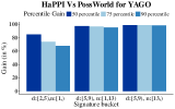
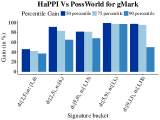
Figure 3. Percentile gains of HaPPI against PossWorld.

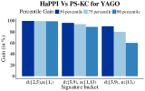
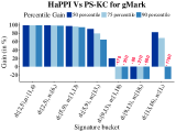
Figure 4. Percentile gains of HaPPI against PS-KC.

Percentile Gains

We dig deeper to analyze the gains of HaPPI over the other two systems in more detail. Timing averages of exponential systems tend to be dominated by corner cases. To guard against that, and to get a better insight, we employ a new metric for comparison based on percentile gains. By reporting a $p^{\text{th}}$ percentile gain of $x\%$, we mean that for $p\%$ of the answers, HaPPI took at least $x\%$ lesser time than the method compared against. The gain is computed using the following ratio:

$$\text{gain}_{\text{method}}=(\text{time}_{\text{method}}-\text{time}_{\textsc{HaPPI}})/\text{time}_{\text{method}}$$

For instance, Fig. 3 reports a $50^{\text{th}}$ percentile gain of $82\%$ for HaPPI over PossWorld for the bucket $d\in[2,5)$, $n\geq 1$. This means that for $50\%$ of the answers in this bucket, the probability computation time of HaPPI is at most $100-82=18\%$ of the corresponding time of PossWorld. A negative gain indicates that HaPPI is slower. HaPPI shows superior performance across all signature buckets. Fig. 4 shows that the better performance of HaPPI over PS-KC for small answer signatures is uniform inside the buckets with little deviation even for corner cases. The asymptotic deterioration of HaPPI is also visible. There is an exception to this trend. We discuss the unexpected gains in the bucket $d\in[13,16)$, $n\geq 1$ in Sec. 6.3.

6.3. Adaptive Framework

While HaPPI outperforms PS-KC and PossWorld significantly for lower ranges of $d$ and $n$, it is quite slow for larger values. Since PS-KC takes roughly the same amount of time to compute probabilities for the very smallest of query answers to the largest, an adaptive strategy involving both HaPPI and PS-KC seems to be the best. The adaptive strategy utilizes the best of both the worlds: it employs HaPPI for lower ranges of $d$ and $n$, and switches to PS-KC when these parameters become large. We report $3$ bounds, $O(2^{d})$, $O(d\cdot 2^{n})$ and $O(n^{s-n})$, on the probability computation of HaPPI (Sec. 5.3). We, thus, expect to use HaPPI for small values of $d$, $n$ or $s-n$.

To notice the $s-n$ dependence, we need to look at higher values of $d$ and $n$, since HaPPI would outperform PS-KC anyway for smaller values. For the range $13\leq d<16$, this is precisely what happens. Closer inspection showed that $2089$ out of $2415$ answers in this range had signatures $(5,21,7)$ or $(7,15,9)$ and HaPPI outperformed PS-KC for all these answers. This explains the aberrant percentile gain of HaPPI. It also empirically validates our analysis on $s-n$ values.

We now elaborate on our adaptive strategy. For each answer, we use HaPPI if one of these $3$ conditions is satisfied: (a) $d<10$, (b) $n<8$, or (c) $n-s<3$. We refer to this signature range as the HaPPI domain of answers. We employ PS-KC outside this domain.

The overall probability computation time of adaptive (HaPPI/PS-KC) and pure PS-KC techniques for YAGO2 and gMark queries are reported under column ‘Computation Time’ in Table 8 and Table 9 respectively. We have also reported the percentage of query answers for which HaPPI was used in the adaptive system. For YAGO2 queries, our adaptive approach is on an average $303$ times faster than pure PS-KC. For gMark queries, we record an average speed-up of $317$ times. The speed-up is, as expected, very high for queries $Q_{32},Q_{35},Q_{54}$, where HaPPI is used for all the query answers. Importantly, the adaptive system gives a $21\%$ speed-up for even $Q_{46}$ where HaPPI is used for only about $37\%$ of the answers and the answer signatures go up to $d=24580$ and $n=8681$.

Table 8. Performance of adaptive system (in $\mu$seconds) for query computation and maintenance for YAGO2 query set.

QId	HaPPI	Computation Time		Gain	Maintenance Time		Gain
	answer %	Adaptive	PS-KC		Recompute	Incremental
$Q_{1}$	$100.00$	$2.7\times 10^{2}$	$6.9\times 10^{4}$	$0.99$	$6.99\times 10^{2}$	$6.29\times 10^{2}$	$0.100$
$Q_{3}$	$99.86$	$2.1\times 10^{4}$	$1.4\times 10^{6}$	$0.98$	$3.26\times 10^{4}$	$2.43\times 10^{4}$	$0.256$
$Q_{6}$	$100.00$	$3.9\times 10^{3}$	$2.3\times 10^{6}$	$0.99$	$1.44\times 10^{4}$	$1.11\times 10^{4}$	$0.226$

Table 9. Performance of adaptive system (in $\mu$seconds) for query computation and maintenance for gMark query set.

QId	HaPPI	Computation Time		Gain	Maintenance Time		Gain
	answer %	Adaptive	PS-KC		Recompute	Incremental
$Q_{4}$	$100.00$	$5.5\times 10^{5}$	$1.0\times 10^{7}$	$0.94$	$6.2\times 10^{5}$	$5.6\times 10^{5}$	$0.097$
$Q_{6}$	$91.47$	$4.1\times 10^{5}$	$3.9\times 10^{6}$	$0.89$	$4.7\times 10^{5}$	$4.4\times 10^{5}$	$0.060$
$Q_{9}$	$94.32$	$1.5\times 10^{4}$	$2.6\times 10^{5}$	$0.94$	$2.0\times 10^{4}$	$1.8\times 10^{4}$	$0.095$
$Q_{21}$	$98.78$	$6.8\times 10^{4}$	$3.5\times 10^{5}$	$0.81$	$1.4\times 10^{5}$	$1.3\times 10^{5}$	$0.091$
$Q_{23}$	$98.88$	$1.1\times 10^{5}$	$8.8\times 10^{6}$	$0.98$	$9.1\times 10^{4}$	$7.8\times 10^{4}$	$0.14$
$Q_{32}$	$100.00$	$1.5\times 10^{2}$	$2.4\times 10^{5}$	$0.99$	$1.5\times 10^{3}$	$1.3\times 10^{3}$	$0.12$
$Q_{35}$	$100.00$	$5.1\times 10^{1}$	$8.0\times 10^{4}$	$0.99$	$7.1\times 10^{2}$	$6.0\times 10^{2}$	$0.16$
$Q_{38}$	$92.45$	$2.1\times 10^{6}$	$2.1\times 10^{7}$	$0.90$	$2.3\times 10^{6}$	$2.2\times 10^{6}$	$0.05$
$Q_{46}$	$36.92$	$3.6\times 10^{7}$	$4.6\times 10^{7}$	$0.21$	$3.7\times 10^{7}$	$3.6\times 10^{7}$	$0.005$
$Q_{54}$	$100.00$	$4.7\times 10^{3}$	$8.5\times 10^{5}$	$0.99$	$1.7\times 10^{4}$	$1.3\times 10^{4}$	$0.24$
$Q_{90}$	$52.27$	$1.2\times 10^{5}$	$1.5\times 10^{5}$	$0.20$	$1.2\times 10^{5}$	$1.2\times 10^{5}$	$0.008$

6.4. Maintenance Time

Next we evaluate the maintainability of HaPPI. Notice that in our maintenance algorithms (Sec. 5.2) we make use of the incremental build-up of the symbolic probability expressions in our semiring only for the case of edge addition. When an edge is deleted we simply recompute the probability expression from scratch. Similarly, updating the probability value for an edge does not affect the already computed symbolic expression for the probability of any answer. Thus, we focus on handling edge insertions in the KG.

Addition of an Edge

When quoting maintenance times for our adaptive system we use HaPPI incrementally on the answers that lie in its domain and do a full re-computation with PS-KC on the rest. This is compared against re-computation with the adaptive system (HaPPI and PS-KC in their respective domains) for all answers. We investigated the effect of the addition of an edge on each individual answer. For every answer, we randomly selected an edge that affects the answer. The sum total of the times taken to incrementally update individual answers (Incremental) for each query is reported in Table 8 and Table 9. This is contrasted against the sum total of the re-computation time (Recompute) for each individual answer under the specific edge addition.

We also report, in the same tables, the percentage of answers for the entire query that are computed using HaPPI. Since PS-KC is not maintainable, the necessitated re-computation on the answers for which the adaptive system uses PS-KC markedly pulls down the overall gain for queries with large answers. While we got $10$-$25\%$ gains for queries that use HaPPI for all their answers, we get more than $5\%$ gains for queries where at least $90\%$ of the answers are computed by HaPPI. Thus, the proposed adaptive system inherits the maintainability of HaPPI.

We also investigated the maintainability of HaPPI. We compared, on the HaPPI domain of answers, incremental time (IncrTime) versus re-computation (RecompTime) with HaPPI in Table 10 and Table 11. Notice that addition of an edge can result in a variable number of derivations being added to an answer. Since the incremental algorithm adds one derivation at a time to our symbolic probability expression, its gains over re-computation go down as the average number of added derivations per answer goes up. We report a gain of at least $20\%$ for all queries where average number of derivations added is less than $4$ but greater than $2$. Note that for answers with just $2$ derivations, re-computation is almost equivalent to the iterative step. Thus the gains ($10$-$35\%$) are muted for queries with smaller averages ($<2$). Queries with higher average number of derivations have more modest gains ($8$-$11\%$).

Table 10. Comparison of incremental update time and re-computation time (in $\mu$seconds) for YAGO2 query answers in HaPPI domain.

QId	Average number of derivations affected	RecompTime	IncrTime	Gain
$Q_{1}$	$1.33$	$6.99\times 10^{2}$	$6.29\times 10^{2}$	$0.101$
$Q_{3}$	$1.37$	$2.95\times 10^{4}$	$2.11\times 10^{4}$	$0.284$
$Q_{6}$	$1.55$	$1.44\times 10^{4}$	$1.12\times 10^{4}$	$0.226$

Table 11. Comparison of incremental update time and re-computation time (in $\mu$seconds) for gMark query answers in HaPPI domain.

QId	Average number of derivations affected	RecompTime	IncrTime	Gain
$Q_{4}$	$6.815$	$6.23\times 10^{5}$	$5.62\times 10^{5}$	$0.097$
$Q_{6}$	$2.015$	$9.79\times 10^{4}$	$7.00\times 10^{4}$	$0.285$
$Q_{9}$	$1.530$	$6.98\times 10^{3}$	$5.46\times 10^{3}$	$0.217$
$Q_{21}$	$6.848$	$1.10\times 10^{5}$	$9.70\times 10^{4}$	$0.118$
$Q_{23}$	$1.572$	$3.80\times 10^{4}$	$2.50\times 10^{4}$	$0.342$
$Q_{32}$	$1.000$	$1.48\times 10^{3}$	$1.30\times 10^{3}$	$0.122$
$Q_{35}$	$1.433$	$7.12\times 10^{2}$	$5.95\times 10^{2}$	$0.164$
$Q_{38}$	$1.320$	$3.29\times 10^{5}$	$2.27\times 10^{5}$	$0.310$
$Q_{46}$	$2.633$	$5.28\times 10^{5}$	$3.28\times 10^{5}$	$0.379$
$Q_{54}$	$2.048$	$1.67\times 10^{4}$	$1.27\times 10^{4}$	$0.239$
$Q_{90}$	$4.267$	$1.01\times 10^{4}$	$9.31\times 10^{3}$	$0.078$

7. Conclusions

In this paper we have proposed a novel commutative semiring which enables us to symbolically compute probability of query answers over probabilistic knowledge graphs. Further, we present a framework HaPPI that uses the proposed semiring to support query processing and answer probability maintenance over probabilistic KG. We have compared the efficiency of our proposed probability computation technique against two standard approaches used for probabilistic inference. HaPPI outperforms current systems in a range of queries answer parameters containing almost $70\%$ of the query answers. We have also shown that an adaptive approach that uses HaPPI in conjunction with a knowledge compilation based technique for large query answers is a significantly faster alternative for probabilistic inference.

Appendix A Proof of Theorem 1

The following facts about the function $flat$ are easy to prove and will be used later.

Lemma 0.

For integer polynomials $f$ and $g$,

$$\overline{\overline{f}} =\overline{f}$$

$$\overline{f+g} =\overline{f}+\overline{g}$$

$$\overline{\overline{f}g} =\overline{fg}$$

We now prove our main theorem

Theorem 2.

$(Z_{F}[p_{1},p_{2},\ldots,p_{n}],\oplus,\otimes,0,1)$ is a commutative semiring.

Proof.

That $(Z_{F}[p_{1},p_{2},\ldots,p_{n}],\otimes)$ is a commutative monoid with identity $1$ follows directly from the definitions.

The operator $\oplus$ is also clearly commutative and $0$ is an identity for it. To show that $\oplus$ is associative, consider $f,g,h\in Z_{F}[p_{1},p_{2},\ldots,p_{n}]$

$$(f\oplus g)\oplus h =(f+g-\overline{fg})\oplus h$$

$$=f+g-\overline{fg}+h$$

$$\mathrel{\phantom{=}}-\overline{fh+gh-h\times flat(fg})$$

$$=f+g+h-\overline{fg+fh+gh}$$

$$\mathrel{\phantom{=}}+\overline{h\times\overline{fg}}$$

$$=f+g+h-\overline{fg+fh+gh}+\overline{fgh}$$

(by symmetry) $$=(g\oplus h)\oplus f$$

$$=f\oplus(g\oplus h)$$

This equality chain is just a repeated application of Lemma 1.

Since $0\otimes f=f\otimes 0=0$ follows directly by definition, we are only left to show distributivity of $\otimes$ over $\oplus$. We prove a quick lemma before we prove distributivity.

Lemma 0.

For all $f\in Z_{F}[p_{1},p_{2},\ldots,p_{n}]$,

$$f\otimes f=f$$

Proof.

Given the definition of $Z_{F}[p_{1},p_{2},\ldots,p_{n}]$ we prove this by structural induction.

By definition of the $\otimes$ operator, $1\otimes 1=1$ and $p_{i}\otimes p_{i}=p_{i}$ for all $0\leq i\leq n$

It is enough to show that if $g,h\in Z_{F}[p_{1},p_{2},\ldots,p_{n}]$ are such that $g\otimes g=g$ and $h\otimes h=h$ then

$$(g\otimes h)\otimes(g\otimes h)=g\otimes h$$

and

$$(g\oplus h)\otimes(g\oplus h)=g\oplus h$$

Liberally rewriting using Lemma 1 and using $g\otimes g=\overline{g^{2}}=g$ and $h\otimes h=\overline{h^{2}}=h$ from our hypothesis, we get

$$(g\otimes h)\otimes(g\otimes h) =\overline{\overline{gh}\times\overline{gh}}$$

$$=\overline{g^{2}h^{2}}$$

$$=\overline{\overline{g^{2}}\times\overline{h^{2}}}$$

$$=\overline{gh}=g\otimes h$$

and

$$(g\oplus h)\otimes(g\oplus h) =(g+h-\overline{gh})\otimes(g+h-\overline{gh})$$

$$=\overline{g^{2}+h^{2}+2gh-2g\overline{gh}-2h\overline{gh}+(\overline{gh})^{2}}$$

$$=\overline{g^{2}}+\overline{h^{2}}+2\overline{gh}-2\overline{g\overline{gh}}-2\overline{h\overline{gh}}+\overline{\overline{gh}^{2}}$$

$$=g+h+2\overline{gh}-2\overline{g^{2}h}-2\overline{gh^{2}}+\overline{\overline{g^{2}h^{2}}}$$

$$=g+h+2\overline{gh}-2\overline{\overline{g^{2}}h}-2\overline{g\overline{h^{2}}}+\overline{\overline{g^{2}}\times\overline{h^{2}}}$$

$$=g+h+2\overline{gh}-2\overline{gh}-2\overline{gh}+\overline{gh}$$

$$=g+h-\overline{gh}$$

$$=g\oplus h$$

∎

To wrap up our proof of theorem 2, we now prove left distributivity of $\otimes$ over $\oplus$. For $f,g,h\in Z_{F}[p_{1},p_{2},\ldots,p_{n}]$

$$f\otimes(g\oplus h) =\overline{f(g+h-\overline{gh})}$$

$$=\overline{fg}+\overline{fh}-\overline{f\overline{gh}}$$

$$=\overline{fg}+\overline{fh}-\overline{\overline{f^{2}}\times\overline{gh}}$$

$$=\overline{fg}+\overline{fh}-\overline{fg\times fh}$$

$$=\overline{fg}+\overline{fh}-\overline{\overline{fg}\times\overline{fh}}$$

$$=\overline{fg}\oplus\overline{fh}=(f\otimes g)\oplus(f\otimes h)$$

∎

∎

References

- (1)
- Agrawal et al. (2006) Parag Agrawal, Omar Benjelloun, Anish Das Sarma, Chris Hayworth, Shubha Nabar, Tomoe Sugihara, and Jennifer Widom. 2006. Trio: A system for data, uncertainty, and lineage. PVLDB (demonstration) (2006).
- Angles et al. (2020) Renzo Angles et al. 2020. The LDBC Social Network Benchmark. arXiv 2001.02299. arXiv:2001.02299 [cs.DB]
- Bagan et al. (2017) Guillaume Bagan, Angela Bonifati, Radu Ciucanu, George H. L. Fletcher, Aurelien Lemay, and Nicky Advokaat. 2017. GMark: Schema-Driven Generation of Graphs and Queries. IEEE Trans. on Knowl. and Data Eng. (2017).
- Boulos et al. (2005) Jihad Boulos, Nilesh Dalvi, Bhushan Mandhani, Shobhit Mathur, Chris Re, and Dan Suciu. 2005. MYSTIQ: A System for Finding More Answers by Using Probabilities. In SIGMOD.
- Buneman et al. (2001) Peter Buneman, Sanjeev Khanna, and Tan Wang-Chiew. 2001. Why and where: A characterization of data provenance. In ICDT.
- Cavallo and Pittarelli (1987) Roger Cavallo and Michael Pittarelli. 1987. The Theory of Probabilistic Databases. In VLDB.
- Cyganiak (2005) Richard Cyganiak. 2005. A relational algebra for SPARQL. Technical Report HPL-2005-170. HP Laboratories.
- Dalvi and Suciu (2007a) Nilesh Dalvi and Dan Suciu. 2007a. Efficient Query Evaluation on Probabilistic Databases. The VLDB Journal 16 (2007).
- Dalvi and Suciu (2007b) Nilesh N. Dalvi and Dan Suciu. 2007b. The dichotomy of conjunctive queries on probabilistic structures. In PODS. 293–302.
- Darwiche (2004) Adnan Darwiche. 2004. New Advances in Compiling CNF to Decomposable Negation Normal Form. In ECAI.
- Darwiche and Marquis (2002) Adnan Darwiche and Pierre Marquis. 2002. A Knowledge Compilation Map. J. Artif. Int. Res. 17, 1 (Sept. 2002), 229–264.
- den Broeck and Suciu (2017) Guy Van den Broeck and Dan Suciu. 2017. Query Processing on Probabilistic Data: A Survey. Found. Trends Databases 7 (2017).
- Deshpande and Sarawagi (2007) Amol Deshpande and Sunita Sarawagi. 2007. Probabilistic Graphical Models and their Role in Databases. In VLDB.
- Dey and Sarkar (1996) Debabrata Dey and Sumit Sarkar. 1996. A Probabilistic Relational Model and Algebra. ACM Trans. Database Syst. 21 (1996).
- Fader et al. (2011) Anthony Fader, Stephen Soderland, and Oren Etzioni. 2011. Identifying Relations for Open Information Extraction. Association for Computational Linguistics (ACL).
- Fuhr and Rölleke (1997) Norbert Fuhr and Thomas Rölleke. 1997. A Probabilistic Relational Algebra for the Integration of Information Retrieval and Database Systems. ACM Trans. Inf. Syst. 15 (1997).
- Gatterbauer and Suciu (2017) Wolfgang Gatterbauer and Dan Suciu. 2017. Dissociation and Propagation for Approximate Lifted Inference with Standard Relational Database Management Systems. Springer-Verlag, Berlin, Heidelberg, 5–30.
- Gaur et al. (2017) Garima Gaur, Srikanta J. Bedathur, and Arnab Bhattacharya. 2017. Tracking the Impact of Fact Deletions on Knowledge Graph Queries Using Provenance Polynomials. In CIKM.
- Gaur et al. (2020) Garima Gaur, Arnab Bhattacharya, and Srikanta J. Bedathur. 2020. How and Why is an Answer (Still) Correct? Maintaining Provenance in Dynamic Knowledge Graphs. In CIKM.
- Geerts and Poggi (2010) Floris Geerts and Antonella Poggi. 2010. On database query languages for k-relations. Journal of Applied Logic 8, 2 (2010).
- Green et al. (2007) Todd J. Green, Grigoris Karvounarakis, and Val Tannen. 2007. Provenance Semirings. In PODS.
- Green and Tannen (2006) Todd J. Green and Val Tannen. 2006. Models for Incomplete and Probabilistic Information. In EDBT.
- Harris et al. (2013) Steve Harris, Andy Seaborne, and Eric Prud’hommeaux. 2013. SPARQL 1.1 Query Language: a W3C Recommendation.
- Hoffart et al. (2011) Johannes Hoffart et al. 2011. YAGO2: exploring and querying world knowledge in time, space, context, and many languages. In WWW.
- Hoffart et al. (2013) Johannes Hoffart et al. 2013. YAGO2: A spatially and temporally enhanced knowledge base from Wikipedia. Artificial Intelligence (2013).
- Huang et al. (2009) Jiewen Huang, Lyublena Antova, Christoph Koch, and Dan Olteanu. 2009. MayBMS: A Probabilistic Database Management System. In SIGMOD.
- Jampani et al. (2008) Ravi Jampani, Fei Xu, Mingxi Wu, Luis Leopoldo Perez, Christopher Jermaine, and Peter J. Haas. 2008. MCDB: A Monte Carlo Approach to Managing Uncertain Data. In SIGMOD.
- Karp and Luby (1983) Richard M. Karp and Michael Luby. 1983. Monte-Carlo Algorithms for Enumeration and Reliability Problems. In SFCS. 56–64.
- Lagniez and Marquis (2017) Jean-Marie Lagniez and Pierre Marquis. 2017. An Improved Decision-DNNF Compiler. In IJCAI.
- Mitchell et al. (2015) Tom Mitchell et al. 2015. Never-Ending Learning. In AAAI.
- Muise et al. (2012) Christian Muise, Sheila A. McIlraith, J. Christopher Beck, and Eric I. Hsu. 2012. Dsharp: Fast d-DNNF Compilation with sharpSAT. In Advances in Artificial Intelligence.
- Neumann and Weikum (2010) Thomas Neumann and Gerhard Weikum. 2010. The RDF-3X engine for scalable management of RDF data. The VLDB Journal (2010).
- Olteanu et al. (2009) D. Olteanu, J. Huang, and C. Koch. 2009. SPROUT: Lazy vs. Eager Query Plans for Tuple-Independent Probabilistic Databases. In ICDE. 640–651.
- Re et al. (2007) C. Re, N. Dalvi, and D. Suciu. 2007. Efficient Top-k Query Evaluation on Probabilistic Data. In ICDE.
- Roth (1996) Dan Roth. 1996. On the Hardness of Approximate Reasoning. Artificial Intelligence 82, 1-2 (1996), 273–302.
- Roth and Tan (2013) Mary Roth and Wang-Chiew Tan. 2013. Data Integration and Data Exchange: It’s Really About Time.. In CLDR.
- Sarma et al. (2008) A. D. Sarma, M. Theobald, and J. Widom. 2008. Exploiting Lineage for Confidence Computation in Uncertain and Probabilistic Databases. In ICDE.
- Sen and Deshpande (2007) P. Sen and A. Deshpande. 2007. Representing and Querying Correlated Tuples in Probabilistic Databases. In ICDE.
- Senellart et al. (2018) Pierre Senellart, Louis Jachiet, Silviu Maniu, and Yann Ramusat. 2018. ProvSQL: Provenance and Probability Management in PostgreSQL. PVLDB 11 (2018).
- Singh et al. (2008) Sarvjeet Singh, Chris Mayfield, Sagar Mittal, Sunil Prabhakar, Susanne Hambrusch, and Rahul Shah. 2008. Orion 2.0: Native Support for Uncertain Data. In SIGMOD.
- Wu et al. (2012) Wentao Wu, Hongsong Li, Haixun Wang, and Kenny Q. Zhu. 2012. Probase: A Probabilistic Taxonomy for Text Understanding. In SIGMOD.
- Wylot et al. (2014) Marcin Wylot, Philippe Cudre-Mauroux, and Paul Groth. 2014. TripleProv: Efficient Processing of Lineage Queries in a Native RDF Store. In WWW. 455–466.
- Zimányi (1997) Esteban Zimányi. 1997. Query Evaluation in Probabilistic Relational Databases. In Selected Papers from the International Workshop on Uncertainty in Databases and Deductive Systems.