Combining speakers of multiple languages to improve quality of neural voices

Abstract

In this work, we explore multiple architectures and training procedures for developing a multi-speaker and multi-lingual neural TTS system with the goals of a) improving the quality when the available data in the target language is limited and b) enabling cross-lingual synthesis. We report results from a large experiment using 30 speakers in 8 different languages across 15 different locales. The system is trained on the same amount of data per speaker. Compared to a single-speaker model, when the suggested system is fine tuned to a speaker, it produces significantly better quality in most of the cases while it only uses less than $40\%$ of the speaker’s data used to build the single-speaker model. In cross-lingual synthesis, on average, the generated quality is within $80\%$ of native single-speaker models, in terms of Mean Opinion Score.

Index Terms: multi-speaker synthesis, multilingual synthesis, fine-tuning, neural speech synthesis

1 Introduction

The quality of synthetic speech has improved dramatically since the development of methods based on neural networks, [1, 2]. However, using this technology requires high computational capacity and large amounts of training data. Several researchers have shown that unlike unit-selection text-to-speech (USEL), neural TTS can compensate for the lack of speech data from the target speaker by adding data from other speakers. Most of the research published in this respect has used support speakers in the same language as the target. However, the most common case when developing TTS voices for a new language is that there are no additional supporting speakers in that new language. In that context, the only available options are to record more speakers and/or to use support speakers from different languages.

In this paper, we show the results of applying the latter approach on a large-scale experiment involving 30 target speaker in 8 languages across 15 different locales. Our goal was to address the following questions: a) how effective is it to combine speakers from different languages compared with just training only on the data of the target speaker; b) what type of model architecture and training protocol yields the best quality when using multilingual data; and c) to which extent can the voices created in this way speak some of the other languages included in the training data?

In addition to the standard numerical results, we also show the analysis of the most common errors pointed out by the evaluation subjects. We believe that the results of these experiments will be useful for researchers and practitioners developing synthetic voices.

The structure of the paper is as follows. Section 2 reviews the recent literature on using data from other speakers to create new voices and on the application of this method to create polyglot voices. Section 3 describes the architecture of the models used in the experiment as well as the way in which these models were trained. Section 4 describes the conditions and results of our experiments. It also shows the analysis of most commonly mentioned mistakes for each of the systems. Section 5 discusses some of the results and suggests some possible future directions. Finally, in section 6 conclusions are drawn..

2 Related work

The idea of using data from other speakers to improve the quality of synthetic speech has been explored extensively [3, 4, 5]. Although there has been some work in training multi-speaker text-to-wave models [6], most of the recent work has been in phone-to-spectrogram. For instance, in [7] the effect of reducing the amount of data from the target speaker and compensating for it with data from other speakers was studied. The effect of having imbalanced training data was further analized in [8]. Even more extreme examples were presented in [9], where only 5 minutes of speech were used to get high quality or even in [10] where a single utterance is used. When there are not sufficient support speakers, some authors have suggested to artificially expand the number of training speakers [11] or making use of low quality data [12].

Mixing languages has also been widely studied, although in most cases with the goal of creating polyglot voices. Within the sequence-to-sequence framework, [13] and [14] introduced several modifications to allow training polyglot voices using only monolingual speakers. A non sequence-to-sequence model was proposed in [15].

Even without aiming to create polyglot voices, using compensatory data from speakers in other languages is also a potential solution to the lack of data. However, this option has received less attention. An architecture inspired by the speaker and language factorisation (SLF) approach [16] but within the DNN/LSTM framework was proposed in [17]. Other authors have also shown that mixing data from multiple speakers and languages can yield equal or even better quality than single speaker models [18, 19]. Finally, in [20], 8 Indian languages were combined directly in a very similar way to the one we suggest here but using a DeepVoice3 [21] architecture.

3 Model training

3.1 Model architecture

The basic architecture of our models is Tacotron2 [2]. The main input is a sequence of phones and punctuation marks and the output is a sequence of 80-dimensional mel-spectrogram features. These are computed from speech signals with a sampling rate of 24kHz, using a 25ms analysis window and the Mel filter-bank generated using Librosa Toolkit [22]. An end-pointing flag was also concatenated with the mel-spectrogram vector to make the final 81-dimensional output vectors.

The encoder consists of a look-up table that converts the sequence of phone-IDs into a sequence of 512-dimensional vectors, three 1D-CNNs and one bi-LSTM layers. The attention is a stepwise monotonic attention [23]. On the decoder side, the pre-net consists of two fully connected (FF) layers. The decoder itself is formed by two LSTMs followed by one FF layer to decode the mel-spectrograms and another one to generate the end-pointing signal. These mel-spectrograms are finally passed through a post-net module consisting of 5 1D-CNNs. The training loss combines the L1 for the end-pointing and the output of the decoder, and an L2 for the output of the post-net. For each output step, two output vectors were generated.

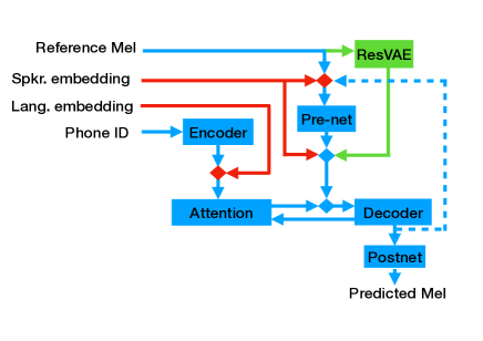
Figure 1: Model architectures. The rhombi indicate concatenation. The dotted line linking the postnet output to the pre-net input is used only at inference time

On top of that standard architecture, two variants were built, as depicted in fig. 1 The first variant (in green) consists of adding a 16-dimensional residual variational auto-encoder (resVAE) following [13]. The main goal of the resVAE is to normalise differences between the utterances that cannot be described from the input. The resVAE consists of 6 2D-CNN layers, each followed by batch normalisation, a GRU, a common FF layer and 2 additional FF layers, one for the mean and another for the covariance diagonal. A sample from this single Gaussian distribution is then concatenated at the input of the decoder. As usual, an additional loss factor for the KLD w.r.t a diagonal Gaussian was added. During inference the resVAE network is bypassed and a constant 0-vector is used instead.

The second variant (in red) is the addition of speaker and language embeddings. The speaker embedding (SE) consists of a 128 dimensional d-vector obtained from a speaker verification model [12]. One advantage of using speaker embeddings versus one-hot is that we can have different values for each utterance. Unfortunately, the SE of each utterance also contains information about the acoustics of that utterance [24]. To avoid this and simulate something akin to a VAE, a single Gaussian model of the embeddings of each speaker was computed and sampled during training. At inference, the mean of the Gaussian was used. The language embeddings (LE) are 32 dimensional vectors obtained from a one hot encoding of the locale associated with each speaker.

We experimented with different ways of adding SE and LE. For SE, we found that the best option is to insert it both at the input of the decoder, concatenated with the output of the attention and with the output of the pre-net as in [25]. This configuration yields the best results in terms of quality, voice similarity to the target speaker and voice consistency when synthesising mix-lingual sentences. For LE, the best option was to concatenate it with the output of the encoder before the attention. Concatenating LE at the beginning of the encoder or after the attention made the models’ training unstable. In any case, the effect of LE was almost negligible, presumably because the phonetic sequence itself already contains enough information about the language.

Previous internal evaluations on models with SE but without fine tuning showed a preference for adding the resVAE. For that reason, all our models with SE also include resVAE. In some initial models we also included a domain adversarial NN (DANN) loss against the identification of the speaker from the encoder outputs as suggested in [13]. Although DANN provided some good results when mixing only 2-3 languages with at least 4 speakers each [24], it introduced instability when we added languages for which only two speakers were available.

3.2 Training procedure

Models that do not include any speaker information need to be fine-tuned in order to get a stable voice. Models that include SE can be used either directly, as in [7], or they can also be fine-tuned. All the base models were trained on exactly the same data. For the fine-tuning to each target speaker we used exactly the same utterances of that speaker that were used as part of the base-model training. We didn’t consider experiments in which an existing model was fine-tuned to an unseen speaker because if the data for the new speaker is available, it can always be mixed with the existing speakers to create a new base model.

All models were trained on a single GPU with a batch size of 16. We used the Adam optimiser [26] with 0.9 and 0.999 for beta1 and beta2, respectively, an initial learning rate of 0.001, 4000 warm-up steps and “Noam decay scheme” [27]. The seed models were trained for 2.5 million steps and then fine-tuned for another 0.5 million steps. The non fine-tuned seed model with speaker embeddings was further trained up to 4.5 million steps. The systems that were finally evaluated are shown in Table 1 .

Table 1: Evaluated models

System	Fine Tuned (FT)	resVAE	SE+LE	#total steps
FT	Yes	No	No	3x$10^{6}$
FTres	Yes	Yes	No	3x$10^{6}$
FTresSE	Yes	Yes	Yes	3x$10^{6}$
resSE	No	Yes	Yes	4.5x$10^{6}$

3.3 Normalisation of the phonetic transcriptions

We normalised the transcriptions across all locales to share a single unified language-agnostic set of phones based on XSAMPA [28]. Previous experiments had shown that in crosslingual synthesis complex phones such as diphthongs, nasalized vowels, syllabic consonants and affricates, tend to get confused and the synthesis only produces half of the phone. To avoid this problem, we split such complex phones. In this way, diphthongs were split into two vowels, affricates into a closure with no audible release plus a fricative, syllabic consonants into the consonant preceded by schwa, and nasalized vowels into a vowel followed by a velar nasal consonant.

Syllabic stress marks were also added to the vowels of the stressed syllables for all languages. It should be noted that for inlingual synthesis, (in which the spoken language is the same language as that of the target voices) most languages do not need explicit stress marks, especially those languages for which stress is not phonemic. However, we found that in crosslingual synthesis, (which is when the synthesised utterances were in a language other than that of the target voices) the lack of stress marks caused serious intelligibility problems, even in languages which are supposed to have no phonemic stress, such as French. In crosslingual synthesis, the voices tended to apply the stress pattern of its own language, e.g., Spanish voices speaking French tended to put the stress in the penultimate syllable. Such changes of the stress patterns made the parsing of the prosodic words very difficult and thus, affected the intelligibility of the utterances.

4 Experiments

We ran two subjective evaluations, one for inlingual synthesis and another for crosslingual synthesis. All the evaluations were 5 points mean opinion score (MOS) tests conducted via crowdsource on each respective locale. The question asked was “How do you rate the overall quality of the voice?”. Each utterance was evaluated by 15 different subjects and no subject was allowed to judge more than 360 samples. With these settings, the total number of listeners per voice was around 120 for the inlingual experiments and 140 for the crosslingual one.

For each evaluation, raw scores were normalized by z-scoring by subject. Mixed effects linear regression models were fitted to the data with subjects and items (sample content/sentence) as random effects and the synthesis method/voice as the fixed effect. T-tests for pairwise contrasts for each pair of voices/systems provided estimated p-values (with Bonferroni correction for the number of contrasts).

4.1 Data

The models were trained on 30 proprietary voices consisting of two speakers for 15 different locales in 8 languages: Australia, India, Ireland, South Africa, UK and US for English; Mexico and Spain for Spanish; Canada and France for French, Brazil for Portuguese, and Denmark, Germany, Italy and The Netherlands for their respective main languages. From each speaker we used 8500 utterances randomly selected from the total corpus, which on average corresponds to 7.73 hours/speaker. This amount of data corresponds on average to 37% of the data used to train the single speaker (SingSpkr) models.

4.2 Vocoder

In all the experiments, we used speaker-dependent waveRNN neural vocoders [29]. The same vocoder trained on all the data was used for each voice across all the models. The reasons for this are: a) we only wanted to evaluate differences in the acoustic model and, b) there exist proposals for universal waveRNN that work for both seen and unseen speakers [30, 31]

4.3 Inlingual synthesis

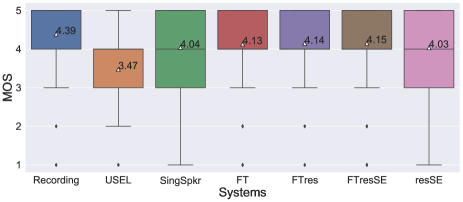
Figure 2: MOS scores across all voices for inlingual synthesis

For each of the 15 locales, 150 utterances were evaluated with each of the 2 speakers’ voices. In addition to the systems described in Table 1, we also evaluated SingSpkr models with the same architecture of FT models, trained from scratch on all the available data of each speaker. The sentences were the same for all the systems but not necessarily the same for both speakers. In order to provide anchors, each evaluation included 50 recorded utterances from each of the target voice talents as the high anchor and the same 150 evaluation sentences generated by a hybrid unit selection system (USEL) [32] as the lower one.

Figure 2 shows the box plot with the summary of the results across all voices. On average, all the fine-tuned models outperformed the SingSpkr models. The average difference between the models is around 0.1 MOS scores. Note that this is by using less than 40% of the target speaker data of the SingSpkr models. Obviously, there are variations depending on the voice. A voice-by-voice analysis is provided in Table LABEL:tab:inlingual_significance_voices. This result confirms that for most voices any of the fine-tuned models perform equal or better than the SingSpkr models. By contrast, resSe was found to be significantly worse than SingSpkr for 11 voices and only better for 4, even though both systems appear to be identical in fig. 2. Our results confirm those reported in [20] for premium voices with 15+ hours of data. Finally, we did not find any significant differences among the 3 fine-tune approaches, although both FTres and FTresSE seem to be marginally better than FT, presumably due to their higher capacity.

Table 2: Number of voices significantly different from SingSpkr models in inlingual synthesis.

	USEL	FT	FTres	FTresSE	resSE
better	1	11	14	14	4
equal	1	18	14	15	15
worse	28	1	2	1	11

4.4 Crosslingual synthesis and evaluation

Our main purpose was to create a base model from which new voices for new languages can be created rapidly. However, given that the seed models are trained on multiple languages, we were curious to know to which extent the fine-tuned models still retained some multilingual capacity. Evaluating each of the 30 voices over the 7 non-native languages would have been ideal, but also very costly. For that reason, we evaluated only the non-native voices when synthesising 4 different foreign languages, American English (en-US), Mexican Spanish (es-MX), France French (fr-FR) and Germany German (de-DE). For each target language 50 utterances from each of the non-native voices were evaluated. Voices in the same main language but from a different locale were not considered. To avoid conflating the differences between native/non-native speakers with those between synthetic/natural speech, we only included as upper anchor 50 utterances generated by the native SingSpkr voice in the target language. These SingSpkr voices are the same as the ones described in Sec. 4.3. To reduce the number of different voices/systems in a single evaluation, the stimuli were split into two groups: one for the voices with the lower median fundamental frequency (F0) and another for the voices with higher median F0 from each locale. This yields a total of 8 independent MOS evaluations. In total, the number of individual voices evaluated on each experiment were 10 for English, 14 for Spanish and French and 15 for German. Subjects were not warned that they were going to listen to foreign accented speech.

Table 3 shows for how many of the 8 evaluations the MOS difference between models were significant, and Table 4 reports the average MOS for each combination of target-language and voice-locale. In general, all systems’ performance is very similar. For most voices the non fine-tuned system resVAE is usually better than the fine-tuned ones. This result is not surprising since fine-tuned models tend to “forget” previous knowledge. However, with the exception of the low-pitch voices in French those differences were not significant. Among the fine-tuned models, FTres and FTresSE were better than FT on average, probably because of the higher capacity introduced by the additional resVAE. However, the addition of the speaker embedding does not seem to provide any advantage when the model is fine-tuned.

Despite these differences, the combination of voice and target language has a much stronger impact over the speech quality than the model type. As shown in Table 4, some combinations achieve scores around 4.0 while others fall below 3.0.

Table 3: Number of model comparisons across the 8 crosslingual evaluations in which the MOS difference was significant

Systems	#$1^{st}$ better	#$2^{nd}$ better	#No diff.
resSE vs. FT	1	0	7
resSE vs. FTres	1	0	7
resSE vs. FTresSE	1	0	7
FT vs. FTres	0	3	5
FT vs. FTresSE	2	6	0
FTres vs. FTresSE	2	2	4

Table 4: Crosslingual MOS per locale. The numbers in the target language column are the average MOS of the two ‘Native SingSpkr’ voices in that language.

Target language	Speaker locale	FT	FTres	FTresSE	resSE
American English 4.2	da-DK	3.77	3.84	3.78	3.7
	de-DE	3.88	3.88	3.96	4.01
	es-ES	3.66	3.74	3.77	3.78
	es-MX	3.81	3.82	3.81	3.93
	fr-CA	3.75	3.82	3.81	3.93
	fr-FR	3.62	3.69	3.72	3.79
	it-IT	3.72	3.69	3.76	3.76
	nl-NL	3.84	3.87	3.85	3.9
	pt-BR	3.68	3.71	3.81	3.88
France French 4.35	da-DK	3.08	3.25	3.26	3.34
	de-DE	3.77	3.84	3.84	3.86
	en-AU	3.08	3.11	3.2	3.42
	en-GB	3.28	3.33	3.3	3.51
	en-IE	3.29	3.32	3.49	3.46
	en-IN	3.46	3.43	3.5	3.7
	en-US	3.27	3.29	3.29	3.57
	en-ZA	3.25	3.47	3.47	3.69
	es-ES	3.37	3.46	3.48	3.67
	es-MX	3.55	3.53	3.58	3.7
	it-IT	3.62	3.54	3.66	3.81
	nl-NL	3.18	3.52	3.32	3.66
	pt-BR	3.27	3.4	3.56	3.72
Mexican Spanish 4.45	da-DK	2.88	3.08	2.87	2.67
	de-DE	3.3	3.35	3.18	3.38
	en-AU	2.94	2.91	2.9	3.04
	en-GB	3.15	2.93	3.02	3.13
	en-IE	3.03	2.98	3.07	3.21
	en-IN	3.34	3.45	3.15	3.32
	en-US	3.24	3.14	3.12	3.14
	en-ZA	2.95	3.08	3.07	3.2
	fr-CA	3.23	3.05	3.09	3.46
	fr-FR	3.41	3.45	3.37	3.47
	it-IT	3.95	4	3.92	3.95
	nl-NL	3.03	3.08	2.85	3.08
	pt-BR	3.63	3.62	3.61	3.64
Germany German 3.96	da-DK	3.27	3.32	3.3	3.3
	en-AU	3.47	3.58	3.57	3.63
	en-GB	3.51	3.51	3.55	3.66
	en-IE	3.57	3.7	3.66	3.82
	en-IN	3.6	3.67	3.6	3.77
	en-US	3.62	3.66	3.52	3.66
	en-ZA	3.66	3.75	3.69	3.8
	es-ES	2.88	3.12	3.09	3.44
	es-MX	3.2	3.29	3.46	3.55
	fr-CA	3.16	3.25	3.28	3.67
	fr-FR	3.34	3.4	3.42	3.59
	it-IT	3.16	3.18	3.12	3.57
	nl-NL	3.43	3.55	3.51	3.65
	pt-BR	2.8	2.97	3.27	3.55
Total		3.39	3.44	3.44	3.57

4.5 Analysis of the comments

In inlingual synthesis, the main problems noted were in terms of pauses (either misplaced or too few), pace (usually too fast), unnatural intonation, and audio quality deterioration. These problems seem to affect more the resSE model. Word stress also seems to be sometimes slightly misplaced in some languages. In the resSE model, some non-phonemic distinctions are also less accurately predicted, e.g., the Italian trill is sometimes chosen instead of the flap.

In crosslingual synthesis, the foreign accent of a voice is usually well identified, but in some cases deemed too pronounced to the extent of impeding intelligibility, especially when in combination with insufficient pausing and fast pace. We also notice a degraded audio quality, affecting some voices more than others, with some occasional “blabber”. Intonation contours are sometimes incorrect and sometimes deemed as monotone. In terms of pronunciation, the model without fine tuning seems to retain less accent and produces a more accurate approximation of the target language phones. This effect is notable, for example, with the American English rhotic and the French voices: the model without fine tuning being the closer to the English alveolar approximant (although getting inaudible in word final position or pre-consonantical position), and other models having a pronunciation closer or identical to the French rhotic. For most voices, lexical stress seems to be placed correctly.

In some language pairs, some phonemic distinctions are lost. For example, the Spanish trill/flap pair is not always maintained when synthesising with French, English, or German voices. The English phone /h/ is often dropped in the synthesis with the French voices. Actually, human French speakers often do drop that phoneme. However, it contributes to the impression of strong foreign accent as more proficient speakers would tend to realise it. Another factor contributing to the impression of strong foreign accent is that intonation and some phonological phenomena are ported to the target language. For instance, word final rhotic is dropped by British English voices, and sometimes French voices insert liaison in Spanish. It is also interesting to note that some American English subjects expected a genuine non-native accent. For example, they expected /t/ or /d/ instead of flaps in the French, Portuguese and German voices.

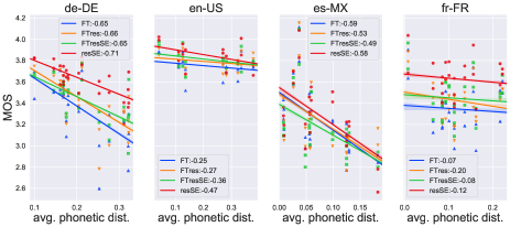
Figure 3: Average crosslingual MOS per voice w.r.t average phonetic distance between voice and language

5 Discussion

5.1 Differences by language

There are two interesting observations from the crosslingual evaluation. The first one is the large variation in the MOS depending on the combination of target voice/language as shown in Table 4. One possible explanation for this is that the phonetic differences between the voice’s language and the target language matters. Figure 3 shows the average MOS of the voices/systems in the crosslingual evaluation with respect to the average phonetic distance between the speaker data and the test sentence of the target computed as

$$AvgPhoneDist=\sum_{\forall t\in T}P(t|T)\min_{\forall s\in S}dist(e_{t},e_{s})$$ (1)

where $T$ and $S$ are the sets of unique phones in the test utterances of the target language and in the target speaker data, respectively; $e_{t}$ and $e_{s}$ denote the phone embeddings for $t$ and $s$ taken from the look-up-table of the resSE model, and $dist$ is the cosine similarity function. Note that for all $t\in S$ the minimum distance is 0.

Figure 3 shows that the impact of the phonetic distance depends on the target language. For instance, Mexican subjects penalised foreign accented voices heavily, even when the average phonetic distance is small. On the contrary, for French subjects other factors seem to be more important. For example, for the British, Australian and Irish English voices, the factors that produce the most negative impact are very unnatural and strongly pronounced intonation, unnatural parsing of groups of words and pace which generally affected intelligibility. For the British English voices, the intelligibility is also affected by the porting of the non-rhotic character of British English to French: final /r/ are often dropped and the quality and length of the previous vowel is modified. The pronunciation of French diaeresis also seems problematic in terms of intelligibility, being realised as a diphthong (as in ”pays” for instance). On the other hand, German, Italian, Portuguese, and Spanish voices were preferred in terms of general intelligibility, even though the intonation was found too monotone, the pauses sometimes incorrectly placed or missing, and the foreign accent too strong.

For American English, MOS is also strongly correlated with the average phonetic distance, but mainly due to the smaller dispersion. Otherwise, the curves are flatter than for German or Spanish. This links with the second observation which is that the average MOS for American English is higher than for the other languages. One explanation of that higher score is that an average of 7% of the 8500 training utterances of the non-English voices were in English, with another 13% having at least one English word. The English proficiency of the voice talents varied greatly, from fully bilingual to very accented. Moreover, the English utterances in the training data of many voices were transcribed using the phones of the voice’s language, which might be the reason for the relatively larger phonetic distances for en-US. Still, that English data seems to have contributed to improve the synthesis of English utterances with non-English voices. Another possible explanation for the higher MOS for American English may be that subjects in that locale (and to some extent in France French too) are more used to listening to foreign accents than their Mexican or German counterparts and therefore, have a larger tolerance for them. Further experiments are needed to confirm which hypothesis is correct.

5.2 Pauses

One of the most commented problems for inlingual synthesis was errors with pausing. Since the model does not include any explicit pause predictor, or part-of-speech tagging, the pause prediction depends entirely on the phonetic transcription and punctuation marks. In single-language models, the network might be able to perform some level of syntactic parsing, for example identify the most common function words. In a multilingual framework, this is harder because the same phonetic sequence might also correspond to a content word in a different language. But also, different languages have different rules regarding the punctuation. So, whereas in some languages it is used mostly to indicate pausing, in others they have a more grammatical function. These kinds of differences are hard to disambiguate by just looking at the phone sequence. Including a LE was expected to help with such language-dependent issues. However, simply concatenating a global LE at the input of the attention didn’t work.

6 Conclusions

This paper confirms that data from speakers in other languages can be used to compensate for the lack of target speaker data. We have presented a large-scale experiment on building neural TTS models by mixing speech from 30 speakers of 15 different locales in 8 different languages. The results show that for the vast majority of voices, fine-tuning a multi-lingual and multi-speaker model produces equal or better quality than single-speaker models trained with more than 2.5 times the amount of speaker-specific data.

An evaluation of these models synthesizing speech in a language different from that of the target speaker has confirmed that the models also preserve good multilingual capability. On average, the MOS on these models in a crosslingual scenario is around 80% of the MOS obtained by inlingual single-speaker native voices. Although this may not be enough for a general stand-alone voice in that language, it is sufficient for code-switching. Our results showed that although non fine-tuned voices are marginally better for crosslingual synthesis, for inlingual synthesis they are generally significantly worse than the fine-tuned ones. Finally, we have presented a qualitative analysis of the main problems identified by subjects during the inlingual and crosslingual evaluations.

References

- [1] A. van den Oord, S. Dieleman, H. Zen, K. Simonyan, O. Vinyals, A. Graves, N. Kalchbrenner, A. Senior, and K. Kavukcuoglu, “WaveNet: A Generative Model for Raw Audio,” in Arxiv, 2016. [Online]. Available: https://arxiv.org/abs/1609.03499
- [2] J. Shen, R. Pang, R. J. Weiss, M. Schuster, N. Jaitly, Z. Yang, Z. Chen, Y. Zhang, Y. Wang, R. Skerrv-Ryan, R. A. Saurous, Y. Agiomvrgiannakis, and Y. Wu, “Natural TTS Synthesis by Conditioning Wavenet on MEL Spectrogram Predictions,” in Proc. ICASSP, 2018, pp. 4779–4783.
- [3] J. Yamagishi, T. Kobayashi, Y. Nakano, K. Ogata, and J. Isogai, “Analysis of Speaker Adaptation Algorithms for HMM-Based Speech Synthesis and a Constrained SMAPLR Adaptation Algorithm,” IEEE Transactions on Audio, Speech, and Language Processing, vol. 17, no. 1, pp. 66–83, 2009.
- [4] V. Wan, J. Latorre, K. Yanagisawa, N. Braunschweiler, L. Chen, M. J. F. Gales, and M. Akamine, “Building HMM-TTS Voices on Diverse Data,” IEEE Journal of Selected Topics in Signal Processing, vol. 8, no. 2, pp. 296–306, 2014.
- [5] Y. Fan, Y. Qian, F. K. Soong, and L. He, “Multi-speaker modeling and speaker adaptation for DNN-based TTS synthesis,” in Proc. ICASSP, 2015, pp. 4475–4479.
- [6] J. Park, K. Zhao, K. Peng, and W. Ping, “Multi-Speaker End-to-End Speech Synthesis,” 2019. [Online]. Available: https://arxiv.org/abs/1907.04462
- [7] J. Latorre, J. Lachowicz, J. Lorenzo-Trueba, T. Merritt, T. Drugman, S. Ronanki, and V. Klimkov, “Effect of Data Reduction on Sequence-to-sequence Neural TTS,” in Proc. ICASSP, 2019, pp. 7075–7079.
- [8] H.-T. Luong, X. Wang, J. Yamagishi, and N. Nishizawa, “Training Multi-Speaker Neural Text-to-Speech Systems using Speaker-Imbalanced Speech Corpora,” 2019. [Online]. Available: https://arxiv.org/abs/1904.00771
- [9] Y. Deng, L. He, and F. Soong, “Modeling Multi-speaker Latent Space to Improve Neural TTS: Quick Enrolling New Speaker and Enhancing Premium Voice,” 2019. [Online]. Available: https://arxiv.org/abs/1812.05253
- [10] E. Cooper, C. Lai, Y. Yasuda, F. Fang, X. Wang, N. Chen, and J. Yamagishi, “Zero-Shot Multi-Speaker Text-To-Speech with State-Of-The-Art Neural Speaker Embeddings,” in Proc. ICASSP, 2020, pp. 6184–6188.
- [11] E. Cooper, C.-I. Lai, Y. Yasuda, and J. Yamagishi, “Can Speaker Augmentation Improve Multi-Speaker End-to-End TTS?” 2020. [Online]. Available: https://arxiv.org/abs/2005.01245
- [12] Q. Hu, E. Marchi, D. Winarsky, Y. Stylianou, D. Naik, and S. Kajarekar, “Neural Text-to-Speech Adaptation from Low Quality Public Recordings,” in Proc. 10th ISCA Speech Synthesis Workshop, 2019, pp. 24–28. [Online]. Available: http://dx.doi.org/10.21437/SSW.2019-5
- [13] Y. Zhang, R. J. Weiss, H. Zen, Y. Wu, Z. Chen, R. Skerry-Ryan, Y. Jia, A. Rosenberg, and B. Ramabhadran, “Learning to Speak Fluently in a Foreign Language: Multilingual Speech Synthesis and Cross-Language Voice Cloning,” in Proc. Interspeech, 2019, pp. 2080–2084.
- [14] M. Chen, M. Chen, S. Liang, J. Ma, L. Chen, S. Wang, and J. Xiao, “Cross-Lingual, Multi-Speaker Text-To-Speech Synthesis Using Neural Speaker Embedding,” in Proc. Interspeech, 2019, pp. 2105–2109.
- [15] I. Himawan, S. Aryal, I. Ouyang, S. Kang, P. Lanchantin, and S. King, “Speaker Adaptation of a Multilingual Acoustic Model for Cross-Language Synthesis,” in Proc. ICASSP, 2020, pp. 7629–7633.
- [16] H. Zen, N. Braunschweiler, S. Buchholz, M. J. F. Gales, K. Knill, S. Krstulovic, and J. Latorre, “Statistical Parametric Speech Synthesis Based on Speaker and Language Factorization,” IEEE Transactions on Audio, Speech, and Language Processing, vol. 20, no. 6, pp. 1713–1724, 2012.
- [17] B. Li and H. Zen, “Multi-Language Multi-Speaker Acoustic Modeling for LSTM-RNN Based Statistical Parametric Speech Synthesis,” in Proc. Interspeech, 2016, pp. 2468–2472.
- [18] Y. Fan, Y. Qian, F. K. Soong, and L. He, “Speaker and language factorization in DNN-based TTS synthesis,” in Proc. ICASSP, 2016, pp. 5540–5544.
- [19] Q. Yu, P. Liu, Z. Wu, S. K. Ang, H. Meng, and L. Cai, “Learning cross-lingual information with multilingual BLSTM for speech synthesis of low-resource languages,” in Proc. ICASSP, 2016, pp. 5545–5549.
- [20] K. R. Prajwal and C. V. Jawahar, “Data-Efficient Training Strategies for Neural TTS Systems,” in 8th ACM IKDD CODS and 26th COMAD. Association for Computing Machinery, 2021, p. 223–227. [Online]. Available: https://doi.org/10.1145/3430984.3431034
- [21] W. Ping, K. Peng, A. Gibiansky, S. O. Arik, A. Kannan, S. Narang, J. Raiman, and J. Miller, “Deep Voice 3: Scaling Text-to-Speech with Convolutional Sequence Learning,” 2018. [Online]. Available: https://arxiv.org/abs/1710.07654
- [22] B. McFee, C. Raffel, D. Liang, D. P. Ellis, M. McVicar, E. Battenberg, and O. Nieto, “librosa: Audio and music signal analysis in python,” in Proceedings of the 14th python in science conference, vol. 8, 2015.
- [23] M. He, Y. Deng, and L. He, “Robust Sequence-to-Sequence Acoustic Modeling with Stepwise Monotonic Attention for Neural TTS,” 2019. [Online]. Available: https://arxiv.org/abs/1906.00672
- [24] S. Maiti, E. Marchi, and A. Conkie, “Generating Multilingual Voices Using Speaker Space Translation Based on Bilingual Speaker Data,” in Proc. ICASSP, 2020, pp. 7624–7628.
- [25] L. Xue, W. Song, G. Xu, L. Xie, and Z. Wu, “Building a Mixed-Lingual Neural TTS System with Only Monolingual Data,” in Proc. Interspeech, 2019, pp. 2060–2064.
- [26] D. P. Kingma and J. Ba, “Adam: A Method for Stochastic Optimization,” 2017.
- [27] A. Vaswani, N. Shazeer, N. Parmar, J. Uszkoreit, L. Jones, A. N. Gomez, L. Kaiser, and I. Polosukhin, “Attention Is All You Need,” 2017.
- [28] J. C. Wells, “Computer-coding the IPA: a proposed extension of SAMPA,” 1995, [Online; accessed 28-January-2018]. [Online]. Available: https://www.phon.ucl.ac.uk/home/sampa/ipasam-x.pdf
- [29] N. Kalchbrenner, E. Elsen, K. Simonyan, S. Noury, N. Casagrande, E. Lockhart, F. Stimberg, A. van den Oord, S. Dieleman, and K. Kavukcuoglu, “Efficient Neural Audio Synthesis,” in Proceedings of the 35th International Conference on Machine Learning, 2018, pp. 2410–2419. [Online]. Available: http://proceedings.mlr.press/v80/kalchbrenner18a.html
- [30] J. Lorenzo-Trueba, T. Drugman, J. Latorre, T. Merritt, B. Putrycz, R. Barra-Chicote, A. Moinet, and V. Aggarwal, “Towards Achieving Robust Universal Neural Vocoding,” in Proc. Interspeech, 2019, pp. 181–185.
- [31] D. Paul, Y. Pantazis, and Y. Stylianou, “Speaker Conditional WaveRNN: Towards Universal Neural Vocoder for Unseen Speaker and Recording Conditions,” in Proc. Interspeech, 2020, pp. 235–239.
- [32] T. Capes, P. Coles, A. Conkie, L. Golipour, A. Hadjitarkhani, Q. Hu, N. Huddleston, M. Hunt, J. Li, M. Neeracher, K. Prahallad, T. Raitio, R. Rasipuram, G. Townsend, B. Williamson, D. Winarsky, Z. Wu, and H. Zhang, “Siri On-Device Deep Learning-Guided Unit Selection Text-to-Speech System,” in Proc. Interspeech, 2017, pp. 4011–4015.