Strichartz estimates for Maxwell equations in media: The partially anisotropic case

Abstract.

We prove Strichartz estimates for solutions to Maxwell equations in three dimensions with rough permittivities, which have less than three different eigenvalues. To this end, Maxwell equations are conjugated to half-wave equations in phase space. We use the Strichartz estimates in a known combination with energy estimates to show the new well-posedness results for quasilinear Maxwell equations.

1. Introduction

In the following Maxwell equations in media in three spatial dimensions, the physically most relevant case (cf. [6, 12]), are analyzed. These describe the propagation of electric and magnetic fields $(\mathcal{E},\mathcal{B}):\mathbb{R}\times\mathbb{R}^{3}\rightarrow\mathbb{R}^{3}\times\mathbb{R}^{3}$, and displacement and magnetizing fields $(\mathcal{D},\mathcal{H}):\mathbb{R}\times\mathbb{R}^{3}\rightarrow\mathbb{R}^{3}\times\mathbb{R}^{3}$. The system of equations is given by

(1) $$\left\{\begin{aligned} \partial_{t}\mathcal{D}&=\nabla\times\mathcal{H}-\mathcal{J}_{e},\quad\nabla\cdot\mathcal{D}&&=\rho_{e},\\ \partial_{t}\mathcal{B}&=-\nabla\times\mathcal{E}-\mathcal{J}_{m},\quad\nabla\cdot\mathcal{B}&&=\rho_{m},\\ \mathcal{D}(0,\cdot)&=\mathcal{D}_{0},\quad\qquad\quad\quad\mathcal{B}(0,\cdot)&&=\mathcal{B}_{0}.\end{aligned}\right.$$

$(\rho_{e},\rho_{m}):\mathbb{R}\times\mathbb{R}^{3}\to\mathbb{R}\times\mathbb{R}$ denote electric and magnetic charges and $(\mathcal{J}_{e},\mathcal{J}_{m}):\mathbb{R}\times\mathbb{R}^{3}\to\mathbb{R}^{3}\times\mathbb{R}^{3}$ electric and magnetic currents. There is no physical evidence for the existence of magnetic charges or magnetic currents, but we include them to highlight a key aspect of the analysis.

The notations follow the previous work [19] on Maxwell equations in two spatial dimensions. We denote space-time coordinates $x=(x^{0},x^{1},\ldots,x^{n})=(t,x^{\prime})\in\mathbb{R}\times\mathbb{R}^{n}$ and the dual variables in Fourier space by $\xi=(\xi^{0},\xi^{1},\ldots,\xi^{n})=(\tau,\xi^{\prime})\in\mathbb{R}\times\mathbb{R}^{n}$.
In this work we supplement Maxwell equations with time-instantaneous material laws, relating $\mathcal{E}$ with $\mathcal{D}$ and $\mathcal{H}$ with $\mathcal{B}$:

(2) $$\begin{split}\mathcal{D}(x)&=\varepsilon(x)\mathcal{E}(x),\quad\varepsilon:\mathbb{R}\times\mathbb{R}^{3}\rightarrow\mathbb{R}^{3\times 3},\\ \mathcal{B}(x)&=\mu(x)\mathcal{H}(x),\quad\mu:\mathbb{R}\times\mathbb{R}^{3}\rightarrow\mathbb{R}^{3\times 3}.\end{split}$$

$\varepsilon$ is referred to as permittivity, and $\mu$ is referred to as permeability. In some cases we shall assume that $\mu\equiv 1$, which means that the considered material is magnetically isotropic. This is a common assumption in nonlinear optics (cf. [17]). Like in the preceding work [19], we want to describe the propagation in possibly anisotropic and inhomogeneous media. We suppose that $\varepsilon$, $\mu$ are matrix-valued function $\varepsilon,\mu:\mathbb{R}\times\mathbb{R}^{3}\rightarrow\mathbb{R}^{3\times 3}$ with $\Lambda_{1},\Lambda_{2}>0$ such that for any $\xi^{\prime}\in\mathbb{R}^{3}$ and $x\in\mathbb{R}\times\mathbb{R}^{3}$

(3) $$\Lambda_{1}|\xi^{\prime}|^{2}\leq\sum_{i,j=1}^{3}\kappa^{ij}(x)\xi_{i}^{\prime}\xi_{j}^{\prime}\leq\Lambda_{2}|\xi^{\prime}|^{2},\quad\kappa^{ij}(x)=\kappa^{ji}(x),\quad\kappa\in\{\varepsilon,\mu\}.$$

The case of diagonal $\varepsilon=\text{diag}(\varepsilon_{1},\varepsilon_{2},\varepsilon_{3})$, $\mu=1_{3\times 3}$ covers the physically relevant case

(4) $$\varepsilon(\mathcal{E})=(1+|\mathcal{E}|^{2})1_{3\times 3}$$

of the Kerr nonlinearity. The permittivity depends on the electric field itself. We denote

(5) $$\mathcal{C}(D)=\begin{pmatrix}0&-\partial_{3}&\partial_{2}\\ \partial_{3}&0&-\partial_{1}\\ -\partial_{2}&\partial_{1}&0\end{pmatrix},\quad P(x,D)=\begin{pmatrix}\partial_{t}1_{3\times 3}&-\mathcal{C}(D)\mu^{-1}\\ \mathcal{C}(D)\varepsilon^{-1}&\partial_{t}1_{3\times 3}\end{pmatrix}.$$

(1) becomes

(6) $$P(x,D)\begin{pmatrix}\mathcal{D}\\ \mathcal{H}\end{pmatrix}=-\begin{pmatrix}\mathcal{J}_{e}\\ \mathcal{J}_{m}\end{pmatrix},\quad\begin{cases}\nabla\cdot\mathcal{D}=\rho_{e},\\ \nabla\cdot\mathcal{B}=\rho_{m}.\end{cases}$$

Like for the two-dimensional Maxwell equations covered in [19], we make use of the FBI transform and analyze the equation in phase space. $P(x,D)$ is conjugated to half-wave equations whose dispersive properties depend on the number of different eigenvalues of $\varepsilon$. This was previously analyzed in the constant-coefficient case by Lucente–Ziliotti [14] and Liess [13]; see also [18, 16]. It was proved that for $\varepsilon(x)\equiv\varepsilon$ satisfying (3), solutions to (6) with $\varepsilon$ having less than three different eigenvalues and $\mu\equiv 1$ decay like solutions to the three-dimensional wave equation. However, if $\varepsilon$ has three different eigenvalues, the decay is weakened to the decay of the two-dimensional wave equation. The fully anisotropic case will be considered separately in [20]. Presently, we prove the first result for variable rough, possibly anisotropic coefficients. Dumas–Sueur [5] previously showed Strichartz estimates for smooth scalar coefficients. In the much easier two-dimensional case the eigenvalues of the symbol are always separated in phase space

$$i(\xi_{0},\xi_{0}-\|\xi^{\prime}\|_{\varepsilon},\xi_{0}+\|\xi^{\prime}\|_{\varepsilon})\text{ for }\|\xi^{\prime}\|_{\varepsilon}\sim 1.$$

$\|\xi^{\prime}\|_{\varepsilon(x)}$ denotes a norm which depends on $\varepsilon(x)$. This separation of the eigenvalues is no longer the case in three dimensions. Roughly speaking, in the isotropic case, the characteristic set is a sphere with multiplicity two and in the partially anisotropic case $\varepsilon(x)=(\varepsilon_{1}(x),\varepsilon_{2}(x),\varepsilon_{2}(x))$, $\varepsilon_{1}(x)\neq\varepsilon_{2}(x)$, $\mu=1_{3\times 3}$ the characteristic set is described by two ellipsoids intersecting at exactly two points. The characteristic sets in the partially anisotropic case for constant coefficients were analyzed in detail for the time-harmonic equations in [18]. The fact that the ellipsoids are intersecting requires a careful choice of eigenvectors, already in the constant-coefficient case, such that the corresponding Fourier multipliers are $L^{p}$-bounded.

It turns out that in the fully anisotropic case $\varepsilon=\text{diag}(\varepsilon_{1},\varepsilon_{2},\varepsilon_{3})$ with $\varepsilon_{1}\neq\varepsilon_{2}\neq\varepsilon_{3}\neq\varepsilon_{1}$, $\mu=1_{3\times 3}$, the characteristic set ceases to be smooth and becomes the Fresnel wave surface with conical singularities. This is classical and was already pointed out by Darboux [3]. The curvature properties were quantified more precisely in [16] (see also [13]). We summarize the properties of the characteristic surface depending on the number of different eigenvalues in Section 2.3.

Below $|D|^{\alpha}$ and $|D^{\prime}|^{\alpha}$ denote Fourier multipliers:

$$(|D|^{\alpha}u)\widehat{(}\xi)=|\xi|^{\alpha}\hat{u}(\xi),\quad(|D^{\prime}|^{\alpha}u)\widehat{(}\xi)=|\xi^{\prime}|^{\alpha}\hat{u}(\xi),$$

and $(\rho,p,q,d)$ is referred to as Strichartz admissible if $d\in\mathbb{Z}_{\geq 2}$, $\rho=d\big{(}\frac{1}{2}-\frac{1}{q}\big{)}-\frac{1}{p}$, $p,q\geq 2$, $\frac{2}{p}+\frac{d-1}{q}\leq\frac{d-1}{2}$, and $(p,q,d)\neq(2,\infty,3)$. We denote the space-time Lebesgue norm of a function $u:\mathbb{R}\times\mathbb{R}^{d}\to\mathbb{R}$ for $1\leq p,q<\infty$ by

$$\|u\|_{L_{t}^{p}L_{x^{\prime}}^{q}}:=\big{(}\int_{\mathbb{R}}\big{(}\int_{\mathbb{R}^{d}}|u(t,x^{\prime})|^{q}dx^{\prime}\big{)}^{\frac{p}{q}}dt\big{)}^{\frac{1}{p}}$$

with the usual modifications if $p=\infty$ or $q=\infty$. We recall the following results about Strichartz estimates for wave equations. The sharp range, i.e., global-in-time Strichartz estimates

$$\||D^{\prime}|^{1-\rho}u\|_{L_{t}^{p}(\mathbb{R};L_{x^{\prime}}^{q}(\mathbb{R}^{d}))}\lesssim\|u_{0}\|_{\dot{H}^{1}(\mathbb{R}^{d})}+\|u_{1}\|_{L^{2}(\mathbb{R}^{d})}$$

for solutions to the Euclidean wave equation

$$\left\{\begin{array}[]{cl}\partial_{t}^{2}u-\Delta u&=0,\quad(t,x)\in\mathbb{R}\times\mathbb{R}^{d},\;d\geq 2,\\ u(0,\cdot)&=u_{0}\in\dot{H}^{1}(\mathbb{R}^{d}),\quad\dot{u}(0,\cdot)=u_{1}\in L^{2}(\mathbb{R}^{d})\end{array}\right.$$

with $(\rho,p,q,d)$ Strichartz admissible was covered by Keel–Tao [10]. First results for rough coefficients are due to H. Smith [21] until Tataru proved the sharp range in a series of papers (cf. [25, 26, 27]); see also Bahouri–Chemin [1] and Klainerman [11]. Tataru recovered the Euclidean Strichartz estimates for $C^{2}$-coefficients (cf. [26]) locally in time and also for coefficients $\|\partial^{2}g^{ij}\|_{L^{1}_{t}L_{x^{\prime}}^{\infty}}<\infty$ (cf. [27]). Strichartz estimates for less regular coefficients require additional derivative loss, if one does not impose additional symmetry assumptions on the coefficients as shown in counterexamples by Smith–Tataru [22]. The Strichartz estimates for coefficients with $\|\partial g\|_{L_{t}^{2}L_{x^{\prime}}^{\infty}}<\infty$ can be used to show local well-posedness results for quasilinear wave equations, which improve on the energy method. In the isotropic case we can recover Strichartz estimates for scalar wave equations with rough coefficients.

Theorem 1.1 ($C^{2}$-Strichartz estimates in the isotropic case).

Let $\varepsilon_{1},\mu_{1}\in C^{2}(\mathbb{R}\times\mathbb{R}^{3};\mathbb{R})$ and suppose that $\varepsilon=\varepsilon_{1}1_{3\times 3}:\mathbb{R}\times\mathbb{R}^{3}\to\mathbb{R}^{3\times 3}$, $\mu=\mu_{1}1_{3\times 3}:\mathbb{R}\times\mathbb{R}^{3}\to\mathbb{R}^{3\times 3}$ satisfy (3). Let $u=(\mathcal{D},\mathcal{H}):\mathbb{R}\times\mathbb{R}^{3}\to\mathbb{R}^{3\times 3}$ with $\nabla\cdot\mathcal{D}=\rho_{e}$ and $\nabla\cdot\mathcal{H}=\rho_{m}$ and $P$ as in (5). Denote $\rho_{em}=(\rho_{e},\rho_{m})$.

If $\|\partial^{2}\varepsilon_{1}\|_{L^{\infty}_{x}}\leq\nu^{4}$, $\|\partial^{2}\mu_{1}\|_{L^{\infty}_{x}}\leq\nu^{4}$, then the following estimate holds:

(7) $$\||D|^{-\rho}u\|_{L^{p}_{t}L_{x^{\prime}}^{q}}\lesssim\nu\|u\|_{L^{2}_{x}}+\nu^{-1}\|Pu\|_{L^{2}_{x}}+\||D|^{-\frac{1}{2}}\rho_{em}\|_{L^{2}_{x}}$$

provided that the right hand-side is finite and $(\rho,p,q,3)$ is Strichartz admissible.

The theorem states that in case of small charges the dispersive properties of wave equations are recovered. Like in the two-dimensional case, note that on the one hand, if

(8) $$\|\rho_{e}\|_{\dot{H}_{x^{\prime}}^{-\frac{1}{2}}}\sim\|\mathcal{D}\|_{\dot{H}_{x^{\prime}}^{\frac{1}{2}}},\quad\|\rho_{m}\|_{\dot{H}_{x^{\prime}}^{-\frac{1}{2}}}\sim\|\mathcal{B}\|_{\dot{H}_{x^{\prime}}^{\frac{1}{2}}},$$

(7) follows from Sobolev embedding. Moreover, we can find stationary solutions $\mathcal{D}=\nabla\varphi$ and $\mathcal{H}=0$ for $\varepsilon=1_{3\times 3}$, which would clearly violate (7) when omitting the contribution of the charges on the right-hand side in (7).

Corresponding Strichartz estimates with additional derivative loss under weaker regularity assumptions on $\varepsilon$ and $\mu$ follow by standard means (cf. [26, 19]). In the following, for $\lambda\in 2^{\mathbb{Z}}$ we denote Littlewood-Paley projections by

$$(S_{\lambda}f)\widehat{(}\xi)=\beta(\lambda^{-1}\|\xi\|)\hat{f}(\xi),\quad(S_{\lambda}^{\prime}f)\widehat{(}\xi)=\beta^{\prime}(\lambda^{-1}\|\xi^{\prime}\|)\hat{f}(\xi),$$

where $\beta:\mathbb{R}\to\mathbb{R}_{\geq 0}$ denotes a radial function, $\text{supp}(\beta)\subseteq B(0,4)\backslash B(0,1/2)$, which satisfies

(9) $$\sum_{\lambda\in 2^{\mathbb{Z}}}\beta(\lambda x)=1\text{ for }x\neq 0.$$

We have the following for $C^{s}$-coefficients:

Theorem 1.2 ($C^{s}$-Strichartz estimates in the isotropic case).

Let $0<s<2$, $\varepsilon_{1},\mu_{1}\in C^{s}(\mathbb{R}\times\mathbb{R}^{3};\mathbb{R})$, $\varepsilon=\text{diag}(\varepsilon_{1},\varepsilon_{1},\varepsilon_{1}),\quad\mu=\text{diag}(\mu_{1},\mu_{1},\mu_{1}):\mathbb{R}\times\mathbb{R}^{3}\to\mathbb{R}^{3\times 3}$ be matrix-valued functions with coefficients in $C^{s}$, $0<s<2$, satisfying (3). Let $u=(\mathcal{D},\mathcal{H}):\mathbb{R}\times\mathbb{R}^{3}\to\mathbb{R}^{3}\times\mathbb{R}^{3}$ with $\nabla\cdot\mathcal{D}=\rho_{e}$ and $\nabla\cdot\mathcal{B}=\rho_{m}$, $P$ as in (5), and write $\rho_{em}=(\rho_{e},\rho_{m})$. Then, the estimate holds

(10) $$\||D|^{-\rho-\frac{\sigma}{2}}u\|_{L_{t}^{p}L_{x^{\prime}}^{q}}\lesssim\nu\|u\|_{L_{x}^{2}}+\nu^{-1}\|Pu\|_{\dot{H}_{x}^{-\sigma}}+\||D|^{-\frac{1}{2}-\frac{\sigma}{2}}\rho_{em}\|_{L_{x}^{2}}$$

provided that the right hand-side is finite, $(\rho,p,q,3)$ is Strichartz admissible,

$$\sigma=\frac{2-s}{2+s},\text{ and }\|(\varepsilon_{1},\mu_{1})\|_{\dot{C}^{s}}\leq\nu^{4}.$$

Moreover, by the arguments from [27, 19], Strichartz estimates for coefficients $\partial_{x}^{2}\varepsilon\in L_{t}^{1}L_{x^{\prime}}^{\infty}$ (cf. [19, Theorem 1.3]) and the inhomogeneous equation (cf. [19, Theorem 1.5]) are proved. We have the following theorem, which is important to treat quasilinear equations.

Theorem 1.3.

Let $\varepsilon_{1},\mu_{1}\in C^{1}(\mathbb{R}\times\mathbb{R}^{3};\mathbb{R})$, and $\varepsilon=\text{diag}(\varepsilon_{1},\varepsilon_{1},\varepsilon_{1}):\mathbb{R}\times\mathbb{R}^{3}\to\mathbb{R}^{3\times 3}$, $\mu=\text{diag}(\mu_{1},\mu_{1},\mu_{1}):\mathbb{R}\times\mathbb{R}^{3}\to\mathbb{R}^{3\times 3}$ be matrix-valued functions, which satisfy (3) and $\partial_{x}^{2}\varepsilon\in L_{t}^{1}L_{x^{\prime}}^{\infty}$, $\partial^{2}_{x}\mu\in L^{1}_{t}L^{\infty}_{x^{\prime}}$. Let $u$, $P$, $\rho_{em}$ be as in Theorem 1.1, and $(\rho,p,q,3)$ be Strichartz admissible. Then, the following estimate holds

(11) $$\begin{split}\||D^{\prime}|^{-\rho}u\|_{L^{p}(0,T;L_{x^{\prime}}^{q})}&\lesssim\nu^{\frac{1}{p}}\|u\|_{L_{t}^{\infty}L_{x^{\prime}}^{2}}+\nu^{-\frac{1}{p^{\prime}}}\|P(x,D)u\|_{L_{t}^{1}L_{x^{\prime}}^{2}}\\ &\quad+T^{\frac{1}{p}}(\||D^{\prime}|^{-1+\frac{1}{p}}\rho_{em}(0)\|_{L_{x^{\prime}}^{2}(\mathbb{R}^{3})}+\||D^{\prime}|^{-1+\frac{1}{p}}\partial_{t}\rho_{em}\|_{L_{t}^{1}L_{x^{\prime}}^{2}}),\end{split}$$

whenever the right hand-side is finite, provided that $\nu\geq 1$, and $T\|\partial_{x}^{2}\varepsilon\|_{L_{t}^{1}L_{x^{\prime}}^{\infty}}+T\|\partial_{x}^{2}\mu\|_{L_{t}^{1}L_{x^{\prime}}^{\infty}}\leq\nu^{2}$.

The reason for additional terms $\||D^{\prime}|^{-1+\frac{1}{p}}\partial_{t}\rho\|_{L_{t}^{1}L_{x^{\prime}}^{2}}$ compared to (7) is that we use Duhamel’s formula in the reductions. For applying the estimates to solve quasilinear equations, $L_{t}^{\infty}L_{x^{\prime}}^{2}$- and $L_{t}^{1}L_{x^{\prime}}^{2}$-norms are to be preferred. We further have to reduce the regularity of $\varepsilon$ to control $\|\partial\varepsilon\|_{L^{p}L^{\infty}}$ for energy estimates. We denote homogeneous Besov spaces by $\dot{B}^{pqr}_{s}$ with norm

$$\|u\|^{r}_{\dot{B}^{pqr}_{s}}=\sum_{\lambda\in 2^{\mathbb{Z}}}\lambda^{rs}\|S_{\lambda}u\|^{r}_{L_{t}^{p}L_{x^{\prime}}^{q}}$$

with the obvious modification for $r=\infty$. For the coefficients of $\varepsilon$, we use the microlocalizable scale of space (cf. [27, 19, 29]):

$$\|v\|_{\mathcal{X}^{s}}=\sup_{\lambda\in 2^{\mathbb{Z}}}\lambda^{s}\|S_{\lambda}v\|_{L_{t}^{1}L_{x^{\prime}}^{\infty}}.$$

Theorem 1.4.

Let $\varepsilon=\text{diag}(\varepsilon_{1},\varepsilon_{1},\varepsilon_{1}),\;\mu=\text{diag}(\mu_{1},\mu_{1},\mu_{1})\in\mathcal{X}^{s}$, $0<s<2$, and $u=(\mathcal{D},\mathcal{H})$, $(\rho,p,q,3)$, and $\sigma$ as in the assumptions of Theorem 1.2. Then, the following estimate holds:

(12) $$\begin{split}\||D|^{-\rho-\frac{\sigma}{p}}u\|_{\dot{B}^{pq\infty}_{0}}&\lesssim\nu^{\frac{1}{p}}\|u\|_{L_{T}^{\infty}L_{x^{\prime}}^{2}}+\nu^{-\frac{1}{p^{\prime}}}\||D|^{-\sigma}Pu\|_{L_{t}^{1}L_{x^{\prime}}^{2}}\\ &\quad+T^{\frac{1}{p}}(\||D^{\prime}|^{-1+\frac{1}{p}-\frac{\sigma}{p}}\rho_{em}\|_{L_{t}^{\infty}L_{x^{\prime}}^{2}}+\||D^{\prime}|^{-1+\frac{1}{p}-\frac{\sigma}{p}}\partial_{t}\rho_{em}\|_{L_{t}^{1}L_{x^{\prime}}^{2}})\end{split}$$

for all $u$ compactly supported in $[0,T]$, and $\nu$, $T$ verifying

$$T^{s}\|(\varepsilon_{1},\mu_{1})\|^{2}_{\mathcal{X}^{s}}\lesssim\nu^{2+s}.$$

Further inhomogeneous Strichartz estimates are proved by similar means as in [19], which is omitted here. In the partially anisotropic case a diagonalization is still possible, but error terms arising from the composition of pseudo-differential operators presently only allow to prove inferior estimates. We show the following:

Theorem 1.5.

Let $\varepsilon=(\varepsilon_{1},\varepsilon_{2},\varepsilon_{2}):\mathbb{R}\times\mathbb{R}^{3}\to\mathbb{R}^{3\times 3}$ satisfy (3), let $u=(\mathcal{D},\mathcal{H})$, $\rho_{em}=(\rho_{e},\rho_{m})$, and $P$ be as in (6). Let $T>0$ and $\delta>0$.

• If $\partial\varepsilon\in L_{T}^{\infty}L_{x^{\prime}}^{\infty}$, then the following estimate holds:

  (13) $$\begin{split}\|\langle D^{\prime}\rangle^{-\rho-\frac{1}{3p}-\delta}u\|_{L^{p}(0,T;L^{q}(\mathbb{R}^{3}))}&\lesssim_{T,\delta}\|u_{0}\|_{L^{2}(\mathbb{R}^{3})}+\|Pu\|_{L_{T}^{1}L_{x^{\prime}}^{2}}\\ &\quad+\|\langle D^{\prime}\rangle^{-\frac{2}{3}}\rho_{em}(0)\|_{L^{2}_{x^{\prime}}}+\|\langle D^{\prime}\rangle^{-\frac{2}{3}}\partial_{t}\rho_{em}\|_{L_{T}^{1}L_{x^{\prime}}^{2}}.\end{split}$$

• If $\partial\varepsilon\in L_{T}^{2}L_{x^{\prime}}^{\infty}$, then the following estimate holds:

  (14) $$\begin{split}\|\langle D^{\prime}\rangle^{-\rho-\frac{1}{2p}-\delta}u\|_{L^{p}(0,T;L^{q}(\mathbb{R}^{3}))}&\lesssim_{T,\delta}\|u_{0}\|_{L^{2}(\mathbb{R}^{3})}+\|Pu\|_{L_{T}^{1}L_{x^{\prime}}^{2}}\\ &\quad+\|\langle D^{\prime}\rangle^{-\frac{3}{4}}\rho_{em}(0)\|_{L^{2}_{x^{\prime}}}+\|\langle D^{\prime}\rangle^{-\frac{3}{4}}\partial_{t}\rho_{em}\|_{L_{T}^{1}L_{x^{\prime}}^{2}}.\end{split}$$

Moreover, the method of proof recovers the estimates from Theorem 1.1 for $\varepsilon_{1}(x)=e_{1}(t,x_{1})$ and $\varepsilon_{2}(x)=e_{2}(t,x_{1})$. In this case the problematic error terms, which arise from composing pseudo-differential operators in the general case, vanish. We have the following:

Theorem 1.6 ($C^{2}$-Strichartz estimates in the structured partially anisotropic case).

Let $\varepsilon=\text{diag}(\varepsilon_{1},\varepsilon_{2},\varepsilon_{2}):\mathbb{R}\times\mathbb{R}^{3}\to\mathbb{R}^{3\times 3}$ satisfy (3) and for $i=1,2$ suppose that

$$\varepsilon_{i}(x_{0},x^{\prime})=e_{i}(x_{0},x_{1})\text{ with }e_{i}\in C^{2}(\mathbb{R}\times\mathbb{R};\mathbb{R}).$$

Let $u=(\mathcal{D},\mathcal{H}):\mathbb{R}\times\mathbb{R}^{3}\to\mathbb{R}^{3}\times\mathbb{R}^{3}$ and set $\mu=1_{3\times 3}$. If $\|\partial^{2}\varepsilon\|_{L^{\infty}_{x}}\leq\nu^{4}$, then the following estimate holds:

$$\||D|^{-\rho}u\|_{L_{t}^{p}L_{x^{\prime}}^{q}}\lesssim\nu\|u\|_{L^{2}_{x}}+\nu^{-1}\|Pu\|_{L^{2}_{x}}+\||D|^{-\frac{1}{2}}\rho_{em}\|_{L^{2}_{x}}$$

provided that the right hand-side is finite and $(\rho,p,q,3)$ is Strichartz admissible.

Strichartz estimates for less regular coefficients like in Theorems 1.2 and 1.3 hold for $C^{s}$-coefficients or $\partial^{2}\varepsilon\in L_{T}^{1}L_{x^{\prime}}^{\infty}$ under structural assumptions.

As in [19], after conjugation of $P(x,D)$ the key ingredient in the proof of Strichartz estimates are estimates for the half-wave equations. We use the following result, shown in [19]:

Proposition 1.7 ([19, Proposition 1.8]).

Let $\lambda\in 2^{\mathbb{N}_{0}},$ $\lambda\gg 1,$ and $d\geq 2$. Assume $\varepsilon=\varepsilon^{ij}(x)$ satisfies $\varepsilon^{ij}\in C^{2}$, $\|\partial^{2}_{x}\varepsilon\|_{L^{\infty}}\leq 1$, and (3). Let $Q(x,D)$ denote the pseudo-differential operator with symbol

$$Q(x,\xi)=-\xi_{0}+\big{(}\varepsilon^{ij}_{\lambda^{\frac{1}{2}}}(x)\xi_{i}\xi_{j}\big{)}^{1/2}.$$

Moreever, let $u:\mathbb{R}\times\mathbb{R}^{d}\to\mathbb{R}$ decay rapidly outside the unit cube and $(\rho,p,q,d)$ be Strichartz admissible. Then, we find the estimates

(15) $$\lambda^{-\rho}\|S_{\lambda}u\|_{L^{p}L^{q}}\lesssim\|S_{\lambda}u\|_{L^{2}}+\|Q(x,D)S_{\lambda}u\|_{L^{2}}$$

to hold with an implicit constant uniform in $\lambda$. For Lipschitz coefficients $\varepsilon^{ij}$ with $\|\partial^{2}_{x}\varepsilon\|_{L^{1}L^{\infty}}\leq 1$, we obtain

(16) $$\lambda^{-\rho}\|S_{\lambda}u\|_{L^{p}L^{q}}\lesssim\|S_{\lambda}u\|_{L^{\infty}L^{2}}+\|Q(x,D)S_{\lambda}u\|_{L^{2}}.$$

We want to use the Strichartz estimates to improve the local well-posedness for quasilinear Maxwell equations:

(17) $$\left\{\begin{array}[]{cl}P(x,D)(\mathcal{D},\mathcal{H})&=0,\quad\nabla\cdot\mathcal{D}=\nabla\cdot\mathcal{H}=0,\\ (\mathcal{D},\mathcal{H})(0)&\in H^{s}(\mathbb{R}^{3};\mathbb{R})^{6},\end{array}\right.$$

where $\varepsilon^{-1}(\mathcal{D})=\psi(|\mathcal{D}|^{2})1_{3\times 3}$, and $\psi:\mathbb{R}_{\geq 0}\to\mathbb{R}_{\geq 1}$ is a smooth monotone increasing function with $\psi(0)=1$. This covers the Kerr nonlinearity $\varepsilon=(1+|\mathcal{E}|^{2})1_{3\times 3}$. The energy method (cf. [8]) yields local well-posedness for $s>5/2$. We also refer to Spitz’s works [23, 24], where Maxwell equations with Kerr nonlinearity were proved to be locally well-posed in $H^{3}(\Omega)$ on domains with suitable boundary conditions. We compute

$$\begin{split}\partial_{t}(\psi(|\mathcal{D}|^{2})\mathcal{D})&=\psi(|\mathcal{D}|^{2})\partial_{t}\mathcal{D}+(2\psi^{\prime}(|\mathcal{D}|^{2})\mathcal{D}\otimes\mathcal{D})\partial_{t}\mathcal{D}=:\tilde{\psi}_{1}(\mathcal{D})\partial_{t}\mathcal{D},\\ \nabla\times(\psi(|\mathcal{D}|^{2})\mathcal{D})&=[\psi(|\mathcal{D}|^{2})\nabla\times+(2\psi^{\prime}(|\mathcal{D}|^{2})(\mathcal{D}\otimes(\mathcal{D}\times\nabla))^{t})]\mathcal{D}=:\tilde{\psi}_{2}(\mathcal{D})\mathcal{D}.\end{split}$$

After a diagonalization in phase space, we shall see that $\tilde{\psi}_{1}(\mathcal{D})$ and $\tilde{\psi}_{2}(\mathcal{D})$ have at most two different eigenvalues.

Passing to the second order systen yields the system of wave equations:

(18) $$\left\{\begin{array}[]{cl}\partial_{t}^{2}\mathcal{D}&=-\nabla\times(\tilde{\psi}_{2}(\mathcal{D})\nabla\times\mathcal{D}),\quad\nabla\cdot\mathcal{D}=\nabla\cdot\mathcal{H}=0,\\ \partial_{t}^{2}\mathcal{H}&=-\nabla\times(\tilde{\psi}_{1}(\mathcal{D})\nabla\times\mathcal{H}).\end{array}\right.$$

We shall first consider the simplified Kerr system, which is obtained by replacing $\tilde{\psi}_{i}$ with $\psi(|\mathcal{D}|^{2})$:

(19) $$\partial_{t}^{2}\mathcal{D}=-\nabla\times(\psi(|\mathcal{D}|^{2})\nabla\times\mathcal{D}),\quad\nabla\cdot\mathcal{D}=0.$$

In this case we can apply the Strichartz estimates for isotropic permittivity to prove the following:

Theorem 1.8 (Local well-posedness for the simplified Kerr system).

(19) is locally well-posed for $s>\frac{13}{6}$.

We remark that we could likewise treat the system

$$\left\{\begin{array}[]{cl}\partial_{t}^{2}\mathcal{D}&=-\nabla\times(\psi(|\mathcal{D}|^{2})\nabla\times\mathcal{D}),\quad\nabla\cdot\mathcal{D}=0,\\ \partial_{t}^{2}\mathcal{H}&=-\nabla\times(\psi(|\mathcal{D}|^{2})\nabla\times\mathcal{H},\quad\nabla\cdot\mathcal{H}=0.\end{array}\right.$$

with the additional estimates for $\mathcal{H}$ being carried out in similar spirit.

In the case of partially anisotropic permittivity, we can use the Strichartz estimates from Theorem 1.5 directly:

Theorem 1.9 (Local well-posedness for Maxwell equations with partially anisotropic permittivity).

Let $\varepsilon^{-1}=\text{diag}(\psi(|\mathcal{D}_{1}|^{2}),1,1)$ with $\psi:\mathbb{R}_{\geq 0}\to\mathbb{R}_{\geq 1}$ smooth, monotone increasing, and $\psi(0)=1$. Then, the Maxwell system

$$\left\{\begin{array}[]{cl}\partial_{t}\mathcal{D}&=\nabla\times\mathcal{H},\quad\nabla\cdot\mathcal{D}=\nabla\cdot\mathcal{H}=0,\\ \partial_{t}\mathcal{H}&=-\nabla\times(\varepsilon^{-1}\mathcal{D}),\;(\mathcal{D}(0),\mathcal{H}(0))\in H^{s}(\mathbb{R}^{3};\mathbb{R}^{6})\end{array}\right.$$

is locally well-posed for $s>9/4$.

In the two-dimensional case we have shown that the derivative loss for Strichartz estimates with rough coefficients is sharp (cf. [19, Section 7]). In the three dimensional case we do not have an example showing sharpness. However, the fact that the derivative loss in the isotropic case matches the loss for second order hyperbolic operators indicates sharpness of the Strichartz estimates in the isotropic case.

Outline of the paper. In Section 2 we introduce further notations and recall well-known bounds for pseudo-differential operators and the FBI transform. In Section 3, we point out how standard localization arguments reduce Theorems 1.1 and 1.3 to a dyadic estimate with frequency truncated coefficients. Then, the symbol is diagonalized to two degenerate and four non-degenerate half wave equations after an additional localization in phase space. We see that the divergence conditions ameliorate the contribution of the degenerate components as in the two-dimensional case. The estimates for the non-degenerate half-wave equations for $\varepsilon$ having less than three eigenvalues are provided by Proposition 1.7. In Section 4 we show the Strichartz estimates in Theorem 1.5 and 1.6 for partially anisotropic permittivities with rough coefficients. In Section 5 we consider quasilinear Maxwell equations and prove Theorems 1.8 and 1.9.

2. Preliminaries

In this section we collect basic facts about pseudo-differential operators and the FBI transform to be used in the sequel.

2.1. Pseudo-differential operators with rough symbols

In the following we clarify the quantization and recall the composition formulae for pseudo-differential operators presently considered. We refer to [7, 28, 29] for further reading.

Recall the standard Hörmander class of symbols:

$$S^{m}_{\rho,\delta}=\{a\in C^{\infty}(\mathbb{R}^{m}\times\mathbb{R}^{m}):|\partial_{x}^{\alpha}\partial_{\xi}^{\beta}a|\lesssim(1+|\xi|)^{m-\rho|\beta|+|\alpha|\delta}\}$$

for $m\in\mathbb{R}$, $0\leq\delta\leq\rho\leq 1$. In the following we obtain pseudo-differential operators via the quantization:

$$a(x,D)f=(2\pi)^{-m}\int_{\mathbb{R}^{m}}e^{ix.\xi}a(x,\xi)\hat{f}(\xi)d\xi.$$

The $L^{p}$-boundedness of $a(x,D)$ with $a\in S^{0}_{1,\delta}$, $0\leq\delta<1$ is standard (cf. [29, Section 0.11]). In the present context of rough coefficients, we shall also consider symbols which are rough in the spatial variable. After a Littlewood-Paley decomposition and a paradifferential decomposition, we can reduce to Hörmander symbols. We record the following quantification of $L^{p}L^{q}$-boundedness for symbols, which are smooth and compactly supported in the fiber variable and possibly rough in the spatial variable:

Lemma 2.1 ([19, Lemma 2.3]).

Let $1\leq p,q\leq\infty$ and $a\in C^{s}_{x}C^{\infty}_{c}(\mathbb{R}^{m}\times\mathbb{R}^{m})$ with $a(x,\xi)=0$ for $\xi\notin B(0,2)$. Suppose that

$$\sup_{x\in\mathbb{R}^{m}}\sum_{0\leq|\alpha|\leq m+1}\|D_{\xi}^{\alpha}a(x,\cdot)\|_{L^{1}_{\xi}}\leq C.$$

Then, we find the following estimate to hold:

$$\|a(x,D)f\|_{L^{p}L^{q}}\lesssim C\|f\|_{L^{p}L^{q}}.$$

We recall the Kohn–Nirenberg theorem on symbol composition. Denote

$$\partial_{x}^{\alpha}=\partial_{x_{1}}^{\alpha_{1}}\ldots\partial_{x_{m}}^{\alpha_{m}}\text{ and }D_{\xi}^{\alpha}=\partial_{\xi}^{\alpha}/(i^{|\alpha|})$$

for $\alpha\in\mathbb{N}_{0}^{m}$.

Theorem 2.2 ([29, Proposition 0.3C]).

Let $m_{1},m_{2}\in\mathbb{R}$, $0\leq\delta_{i}<\rho_{i}\leq 1$ for $i=1,2$. Given $P(x,\xi)\in S^{m_{1}}_{\rho_{1},\delta_{1}}$, $Q(x,\xi)\in S^{m_{2}}_{\rho_{2},\delta_{2}}$, suppose that

$$0\leq\delta_{2}<\rho\leq 1\text{ with }\rho=\min(\rho_{1},\rho_{2}).$$

Then, $(P\circ Q)(x,D)\in OPS^{m_{1}+m_{2}}_{\rho,\delta}$ with $\delta=\max(\delta_{1},\delta_{2})$, and $P(x,D)\circ Q(x,D)$ satisfies the asymptotic expansion

(20) $$(P\circ Q)(x,D)=\sum_{\alpha}\frac{1}{\alpha!}(D_{\xi}^{\alpha}P\partial_{x}^{\alpha}Q)(x,D)+R,$$

where $R:\mathcal{S}^{\prime}\to C^{\infty}$ is smoothing.

Lemma 2.1 quantifies the $L^{p}L^{q}$-bounds for the expansion (20) (see [19, Section 2]). From truncating the expansion to

$$(P\circ Q)(x,D)=\sum_{|\alpha|\leq N}\frac{1}{\alpha!}(D_{\xi}^{\alpha}P\partial_{x}^{\alpha}Q)(x,D)+R_{N}(x,D),$$

we can find error bounds for $R_{N}$ decaying in $\lambda$. This can be proved again by Lemma 2.1. We recall the Calderon–Vaillancourt theorem (cf. [2, 28]) to bound $OPS^{0}_{\rho,\rho}$. The following quantification is due to Kato [9]:

Theorem 2.3 (Calderon–Vaillancourt).

Let $0\leq\rho<1$ and $a(x,\xi)\in S^{0}_{\rho,\rho}(\mathbb{R}^{2d})$ with

$$|\partial_{x}^{\alpha}\partial_{\xi}^{\beta}a(x,\xi)|\leq C(1+|\xi|)^{\rho(|\alpha|-|\beta|)}$$

for $|\alpha|\leq\lfloor\frac{d}{2}\rfloor+1$, $|\beta|\leq\lfloor\frac{d}{2}\rfloor+2$. Then,

$$\|a(x,D)\|_{L^{2}\to L^{2}}\lesssim_{\rho,d}C.$$

2.2. The FBI transform

We shall make use of the FBI transform to conjugate the evolution to phase space (cf. [4, 27]). For $\lambda\in 2^{\mathbb{Z}}$, we define the FBI transform of $f\in L^{1}(\mathbb{R}^{m};\mathbb{C})$ by

$$\begin{split}T_{\lambda}f(z)&=C_{m}\lambda^{\frac{3m}{4}}\int_{\mathbb{R}^{m}}e^{-\frac{\lambda}{2}(z-y)^{2}}f(y)dy,\qquad z=x-i\xi\in T^{*}\mathbb{R}^{m}\equiv\mathbb{R}^{2m},\\ C_{m}&=2^{-\frac{m}{2}}\pi^{-\frac{3m}{4}}.\end{split}$$

The FBI transform is an isometric mapping $T_{\lambda}:L^{2}(\mathbb{R}^{m})\to L^{2}_{\Phi}(T^{*}\mathbb{R}^{m})$ with $\Phi(z)=e^{-\lambda\xi^{2}}$. The range of $T_{\lambda}$ are holomorphic functions, thus there are many inversion formulae. One is given by the adjoint in $L^{2}_{\Phi}$:

$$T_{\lambda}^{*}F(y)=C_{m}\lambda^{\frac{3m}{4}}\int_{\mathbb{R}^{2m}}e^{-\frac{\lambda}{2}(\bar{z}-y)^{2}}\Phi(z)F(z)dxd\xi.$$

By decomposing a function into coherent states, the FBI transform allows us to find an approximate conjugate of pseudo-differential operators. Let $s\geq 0$, $a(x,\xi)\in C^{s}_{x}C^{\infty}_{c}$ be smooth and compactly supported in $\xi$. We assume that

$$a(x,\xi)=0\text{ for }\xi\notin B(0,2).$$

Let $a_{\lambda}(x,\xi)=a(x,\xi/\lambda)$ denote the scaled symbol and $A_{\lambda}=a_{\lambda}(x,D)$ be the corresponding pseudo-differential operator. We have the following asymptotic for analytic symbols:

$$T_{\lambda}A_{\lambda}(x,D)\approx\sum_{\alpha,\beta}(\partial_{\xi}-\lambda\xi)^{\alpha}\frac{\partial_{x}^{\alpha}\partial_{\xi}^{\beta}a(x,\xi)}{|\alpha|!|\beta|!(-i\lambda)^{|\alpha|}\lambda^{|\beta|}}\big{(}\frac{1}{i}\partial_{x}-\lambda\xi)^{\beta}T_{\lambda}.$$

We consider truncations of the asymptotic expansion. For $s\leq 1$, we let

$$\tilde{a}^{s}_{\lambda}=a,$$

and for $1<s\leq 2$, let

$$\tilde{a}^{s}_{\lambda}=a+\frac{1}{-i\lambda}a_{x}(\partial_{\xi}-\lambda\xi)+\frac{1}{\lambda}a_{\xi}(\frac{1}{i}\partial_{x}-\lambda\xi)=a+\frac{2}{\lambda}(\bar{\partial}a)(\partial-i\lambda\xi)$$

with $\partial=\frac{1}{2}(\partial_{x}+i\partial_{\xi})$ and $\bar{\partial}=\frac{1}{2}(\partial_{x}-i\partial_{\xi})$. We define the remainder

$$R^{s}_{\lambda,a}=T_{\lambda}A_{\lambda}-\tilde{a}^{s}_{\lambda}T_{\lambda}.$$

Tataru [25, 26] proved the following approximation result:

Theorem 2.4 ([26, Theorem 5, p. 393]).

Let $0<s\leq 2$, and $a\in C^{s}_{x}C^{\infty}_{c}$. Then,

$$\begin{split}\|R^{s}_{\lambda,a}\|_{L^{2}\to L^{2}_{\Phi}}&\lesssim\lambda^{-\frac{s}{2}},\\ \|(\partial_{\xi}-\lambda\xi)R^{s}_{\lambda,a}\|_{L^{2}\to L^{2}_{\Phi}}&\lesssim\lambda^{\frac{1}{2}-\frac{s}{2}}.\end{split}$$

Moreover, if $a\in X^{1}C^{\infty}_{c}$ with $X^{1}=\{f\in L_{t}^{2}L_{x^{\prime}}^{\infty}\,:\,\partial f\in L_{t}^{2}L_{x^{\prime}}^{\infty}\}$, then

$$\|R^{1}_{\lambda,a}\|_{L^{\infty}L^{2}\to L^{2}_{\Phi}}\lesssim\lambda^{-\frac{1}{2}}.$$

2.3. The characteristic set depending on the permittivity

In this section we summarize the characteristic set of Maxwell equations depending on the number of different eigenvalues of $\varepsilon=\text{diag}(\varepsilon_{1},\varepsilon_{2},\varepsilon_{3})$ and $\mu=\text{diag}(\mu_{1},\mu_{2},\mu_{3})$. For this discussion suppose that $\varepsilon$ and $\mu$ are homogeneous. The partially anisotropic case (and isotropic case as special case) was detailed in [18] and the fully anisotropic case was analyzed in [16].

2.3.1. Isotropic case

For $\mu$ and $\varepsilon$ proportional to the unit matrix we can diagonalize the principal symbol to the diagonal matrix as will be carried out in Section 3:

$$d(x,\xi)=i\text{diag}(\xi_{0},\xi_{0},\xi_{0}-(\varepsilon\mu)^{-\frac{1}{2}}\|\xi^{\prime}\|,\xi_{0}+(\varepsilon\mu)^{-\frac{1}{2}}\|\xi^{\prime}\|,\xi_{0}-(\varepsilon\mu)^{-\frac{1}{2}}\|\xi^{\prime}\|,\xi_{0}+(\varepsilon\mu)^{-\frac{1}{2}}\|\xi^{\prime}\|).$$

This shows that the characteristic set, without the contribution of the charges, is given by

$$\{\xi_{0}^{2}-(\varepsilon\mu)^{-1}\|\xi^{\prime}\|^{2}=0\}$$

with multiplicity two.

2.3.2. Partially anisotropic case

In the case $\varepsilon=\text{diag}(\varepsilon_{1},\varepsilon_{2},\varepsilon_{2})$, $\varepsilon_{1}\neq\varepsilon_{2}$, $\mu=\mu 1_{3\times 3}$ the diagonalization in the constant-coefficient case with $L^{p}$-bounded multipliers is still possible. We obtain the diagonal matrix:

$$d(x,\xi)=i\text{diag}(\xi_{0},\xi_{0},\xi_{0}-\varepsilon_{2}^{-\frac{1}{2}}\|\xi^{\prime}\|,\xi_{0}+\varepsilon_{2}^{-\frac{1}{2}}\|\xi^{\prime}\|,\xi_{0}-\|\xi^{\prime}\|_{\varepsilon},\xi_{0}+\|\xi^{\prime}\|_{\varepsilon})$$

with $\|\xi^{\prime}\|_{\varepsilon}=(\varepsilon_{2}^{-1}\xi_{1}^{2}+\varepsilon_{1}^{-1}\xi_{2}^{2}+\varepsilon_{1}^{-1}\xi_{3}^{2})^{\frac{1}{2}}$. Clearly, we have

$$\varepsilon_{2}^{-\frac{1}{2}}\|\xi^{\prime}\|=\|\xi^{\prime}\|_{\varepsilon}\;\Leftrightarrow\;\xi_{2}^{\prime}=\xi_{3}^{\prime}=0.$$

The characteristic set is given by the sphere

$$(\xi_{0}^{2}-\|\xi^{\prime}\|_{\varepsilon}^{2})(\xi_{0}^{2}-\varepsilon_{2}^{-1}\|\xi^{\prime}\|^{2})=0$$

and describes two ellipsoids, which are smoothly intersecting at the $\xi_{1}$-axis.

2.3.3. Fully anisotropic case

To find the characteristic set in the fully anisotropic case, we symmetrize

$$\begin{pmatrix}i\xi_{0}&-i\mathcal{C}(\xi^{\prime})\mu^{-1}\\ i\mathcal{C}(\xi^{\prime})\varepsilon^{-1}&i\xi_{0}\end{pmatrix}\begin{pmatrix}\hat{\mathcal{D}}\\ \hat{\mathcal{B}}\end{pmatrix}=0$$

by multiplying with the matrix (cf. [16, Proposition 1.3, p. 1835])

$$\begin{pmatrix}i\xi_{0}&i\mathcal{C}(\xi^{\prime})\mu^{-1}\\ -i\mathcal{C}(\xi^{\prime})\varepsilon^{-1}&i\xi_{0}\end{pmatrix}$$

to find

$$\begin{pmatrix}-\xi_{0}^{2}-\mathcal{C}(\xi^{\prime})\mu^{-1}\mathcal{C}(\xi^{\prime})\varepsilon^{-1}&0\\ 0&-\xi_{0}^{2}-\mathcal{C}(\xi^{\prime})\varepsilon^{-1}\mathcal{C}(\xi^{\prime})\mu^{-1}\end{pmatrix}\begin{pmatrix}\hat{\mathcal{D}}\\ \hat{\mathcal{H}}\end{pmatrix}=0.$$

We compute

$$\begin{split}p(\xi)&=\det(-\xi_{0}^{2}-\mathcal{C}(\xi^{\prime})\mu^{-1}\mathcal{C}(\xi^{\prime})\varepsilon^{-1})\\ &=\det(-\xi_{0}^{2}-\mathcal{C}(\xi^{\prime})\varepsilon^{-1}\mathcal{C}(\xi^{\prime})\mu^{-1})=-\xi_{0}^{2}(\xi_{0}^{4}-\xi_{0}^{2}q_{0}(\xi)+q_{1}(\xi))\end{split}$$

with

$$\begin{split}q_{0}(\xi)&=\xi_{1}^{2}\big{(}\frac{1}{\varepsilon_{2}\mu_{3}}+\frac{1}{\mu_{2}\varepsilon_{3}}\big{)}+\xi_{2}^{2}\big{(}\frac{1}{\varepsilon_{1}\mu_{3}}+\frac{1}{\varepsilon_{3}\mu_{1}}\big{)}+\xi_{3}^{2}\big{(}\frac{1}{\varepsilon_{2}\mu_{1}}+\frac{1}{\varepsilon_{1}\mu_{2}}\big{)},\\ q_{1}(\xi)&=\frac{1}{\varepsilon_{1}\varepsilon_{2}\varepsilon_{3}\mu_{1}\mu_{2}\mu_{3}}(\varepsilon_{1}\xi_{1}^{2}+\varepsilon_{2}\xi_{2}^{2}+\varepsilon_{3}\xi_{3}^{2})(\mu_{1}\xi_{1}^{2}+\mu_{2}\xi_{2}^{2}+\mu_{3}\xi_{3}^{2}).\end{split}$$

It [16, Section 3] was proved that the condition for full anisotropy $\varepsilon=\text{diag}(\varepsilon_{1},\varepsilon_{2},\varepsilon_{3})$ and $\mu=\text{diag}(\mu_{1},\mu_{2},\mu_{3})$ is given by

(21) $$\frac{\varepsilon_{1}}{\mu_{1}}\neq\frac{\varepsilon_{2}}{\mu_{2}}\neq\frac{\varepsilon_{3}}{\mu_{3}}\neq\frac{\varepsilon_{1}}{\mu_{1}}.$$

If this fails, then the characteristic set will be like in the isotropic or partially anisotropic case.

If (21) holds, then the characteristic set ceases to be smooth and becomes the Fresnel wave surface with conical singularities.

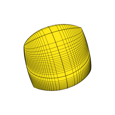
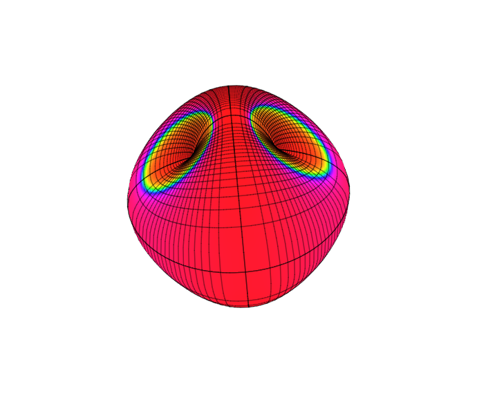
Figure 1. Fresnel surface: inner sheet (left) and outer sheet (right) for $\varepsilon_{1}=1$, $\varepsilon_{2}=3$, $\varepsilon_{3}=9$. The colours on the outer sheet indicate the Gaussian curvature. The Hamiltonian circles with vanishing Gaussian curvature encase the singular points. The images were created with MAPLE^™ with the working sheet [15].

It can be conceived as union of three components:

• a smooth and regular component with two principal curvatures bounded from below,

• one-dimensional submanifolds with vanishing Gaussian curvature and one principal curvature,

• neighbourhoods of (four) conical singularities.

This is classical and was already pointed out by Darboux [3]. The curvature was precisely quantified in [16]. Dispersive properties in the constant-coefficient case were first analyzed by Liess [13]. The conical singularities lead to the dispersive properties of the 2d wave equation. We prove Strichartz estimates for rough coefficients in the companion paper [20].

3. Strichartz estimates in the isotropic case

The purpose of this section is to reduce (1) to half-wave equations in the isotropic case. The Strichartz estimates then follow from Proposition 1.7. The key point is to diagonalize the principal symbol of

$$P(x,D)=\begin{pmatrix}\partial_{t}1_{3\times 3}&-\mathcal{C}(D)\mu^{-1}\\ \mathcal{C}(D)\varepsilon^{-1}&\partial_{t}1_{3\times 3}\end{pmatrix}.$$

The diagonalization argument follows the two-dimensional case, but is more involved. The eigenpairs in the partially anisotropic case had been computed in case of constant coefficients in [18]. This suffices for constant-coefficients, but for variable coefficients this diagonalization appears to lose regularity. However, in the isotropic case, we can find a regular diagonalization after an additional microlocalization.

Further reductions are standard, i.e., reduction to high frequencies and localization to a cube of size $1$, reduction to dyadic estimates, truncating frequencies of the coefficients. We start with diagonalizing the principal symbol:

3.1. Diagonalizing the principal symbol in the isotropic case

We begin with the isotropic case $\varepsilon=\text{diag}(\varepsilon_{1},\varepsilon_{1},\varepsilon_{1})$ and $\mu=\text{diag}(\mu_{1},\mu_{1},\mu_{1})$. In the following we abuse notation and write $\varepsilon=\varepsilon_{1}$ and $\mu=\mu_{1}$ for sake of brevity. In the isotropic case the diagonalization is as regular as in two dimensions after an additional localization in phase space. It turns out we have to distinguish one non-degenerate direction to find non-degenerate eigenvectors.

We use the block matrix structure to find eigenvectors of $p/i$. We have

$$p/i=\begin{pmatrix}\xi_{0}&-\mathcal{C}(\xi^{\prime})\mu^{-1}\\ \mathcal{C}(\xi^{\prime})\varepsilon^{-1}&\xi_{0}\end{pmatrix}\text{ with }\mathcal{C}(\xi^{\prime})_{ij}=-i\varepsilon_{ijk}\xi_{k},$$

where $\varepsilon_{ijk}$ denotes the Levi-Civita symbol.

We find eigenvectors $v=(v_{1},v_{2})\in\mathbb{C}^{3}\times\mathbb{C}^{3}$ by using the block matrix structure of $p/i$. Let $\lambda\in\mathbb{R}$ (note that $p/i$ is symmetric, which yields real eigenvalues) such that

$$\begin{pmatrix}\xi_{0}&-\mathcal{C}(\xi^{\prime})\mu^{-1}\\ \mathcal{C}(\xi^{\prime})\varepsilon^{-1}&\xi_{0}\end{pmatrix}\begin{pmatrix}v_{1}\\ v_{2}\end{pmatrix}=\lambda\begin{pmatrix}v_{1}\\ v_{2}\end{pmatrix}.$$

Let $\lambda^{\prime}=\lambda-\xi_{0}$. Then, we find the system of equations

(22) $$-\mathcal{C}(\xi^{\prime})\mu^{-1}v_{2} =\lambda^{\prime}v_{1},$$

(23) $$\mathcal{C}(\xi^{\prime})\varepsilon^{-1}v_{1} =\lambda^{\prime}v_{2}.$$

In the following let $\xi^{\prime}\neq 0$ because $p$ is already diagonal for $\xi^{\prime}=0$. Denote $\xi_{i}^{*}=\xi_{i}/|\xi^{\prime}|$. Clearly, for $\lambda=\xi_{0}$ we find two eigenvectors

$$\begin{pmatrix}\xi_{1}^{*}&\xi_{2}^{*}&\xi_{3}^{*}&0&0&0\end{pmatrix}^{t},\qquad\begin{pmatrix}0&0&0&\xi_{1}^{*}&\xi_{2}^{*}&\xi_{3}^{*}\end{pmatrix}^{t}$$

because $\text{span}(\xi^{\prime})=\ker(\mathcal{C}(\xi^{\prime}))$. So, in the following suppose that $\lambda\neq\xi_{0}$, and let $\lambda^{\prime}=\lambda-\xi_{0}$. Iterating (22) and (23), we find that $v_{1}$ and $v_{2}$ solve the eigenpair equations:

(24) $$-\mathcal{C}(\xi^{\prime})\mu^{-1}\mathcal{C}(\xi^{\prime})\varepsilon^{-1}v_{1} ={\lambda^{\prime}}^{2}v_{1},$$

(25) $$-\mathcal{C}(\xi^{\prime})\varepsilon^{-1}\mathcal{C}(\xi^{\prime})\mu^{-1}v_{2} ={\lambda^{\prime}}^{2}v_{2}.$$

Since $\varepsilon$ and $\mu$ are isotropic and elliptic, we can define

$$\lambda^{*}=(\varepsilon\mu)^{\frac{1}{2}}\lambda^{\prime},$$

and write (24) and (25) as

$$-\mathcal{C}^{2}(\xi^{\prime})v_{i}={\lambda^{*}}^{2}v_{i},\quad i=1,2.$$

We have $\mathcal{C}^{2}(\xi^{\prime})=-\|\xi^{\prime}\|^{2}1_{3\times 3}+\xi^{\prime}(\xi^{\prime})^{t}$. We note that $\langle v_{i},\xi^{\prime}\rangle=0$, which follows from projecting (24) and (25) to $\xi^{\prime}$ and supposing that $\lambda^{\prime}\neq 0$. We obtain $\lambda^{*}\in\{-\|\xi^{\prime}\|;\|\xi^{\prime}\|\}$. We shall construct eigenvectors depending on the non-degenerate direction of $\xi^{*}=\frac{\xi^{\prime}}{\|\xi^{\prime}\|}\in\mathbb{S}^{2}$. Clearly, there is $i\in\{1,2,3\}$ such that $(\xi_{i}^{*})^{2}\geq\frac{1}{3}$. We introduce the notation $\xi_{ij}^{2}=\xi_{i}^{2}+\xi_{j}^{2}$ for $i,j\in\{1,2,3\}$.

Eigenvectors for $|\xi_{1}^{*}|\gtrsim 1$: We let

$$v_{1}^{(1)}=\begin{pmatrix}\frac{\xi_{2}}{\xi_{12}}\\ -\frac{\xi_{1}}{\xi_{12}}\\ 0\end{pmatrix},\quad v_{2}^{(1)}=\frac{\mathcal{C}(\xi^{\prime})\varepsilon^{-1}}{\lambda^{\prime}}v_{1}^{(1)}=\pm\big{(}\frac{\mu}{\varepsilon}\big{)}^{\frac{1}{2}}\begin{pmatrix}\frac{\xi_{1}\xi_{3}}{\xi_{12}\|\xi^{\prime}\|}\\ \frac{\xi_{2}\xi_{3}}{\xi_{12}\|\xi^{\prime}\|}\\ -\frac{\xi_{12}}{\|\xi^{\prime}\|}\end{pmatrix}.$$

The choice of $v_{2}^{(1)}$ satisfies (23) and is orthogonal to $\xi^{*}$. (22) is satisfied for

$$\lambda^{\prime}\in\{\frac{\|\xi^{\prime}\|}{(\varepsilon\mu)^{\frac{1}{2}}},-\frac{\|\xi^{\prime}\|}{(\varepsilon\mu)^{\frac{1}{2}}}\}.$$

Secondly, we let

$$v_{1}^{(2)}=\begin{pmatrix}\frac{\xi_{3}}{\xi_{13}}\\ 0\\ -\frac{\xi_{1}}{\xi_{13}}\end{pmatrix},\quad v_{2}^{(2)}=\frac{\mathcal{C}(\xi^{\prime})\varepsilon^{-1}}{\lambda^{\prime}}v_{1}^{(2)}=\pm\big{(}\frac{\mu}{\varepsilon}\big{)}^{\frac{1}{2}}\begin{pmatrix}\frac{-\xi_{1}\xi_{2}}{\xi_{13}\|\xi^{\prime}\|}\\ \frac{\xi_{13}}{\|\xi^{\prime}\|}\\ \frac{-\xi_{2}\xi_{3}}{\xi_{13}\|\xi^{\prime}\|}\end{pmatrix}.$$

$v_{1}^{(1)}$ and $v_{1}^{(2)}$ are linearly independent. For the diagonal matrix

(26) $$d(x,\xi)=i\text{diag}(\xi_{0},\xi_{0},\xi_{0}-\frac{\|\xi^{\prime}\|}{(\varepsilon\mu)^{\frac{1}{2}}},\xi_{0}+\frac{\|\xi^{\prime}\|}{(\varepsilon\mu)^{\frac{1}{2}}},\xi_{0}-\frac{\|\xi^{\prime}\|}{(\varepsilon\mu)^{\frac{1}{2}}},\xi_{0}+\frac{\|\xi^{\prime}\|}{(\varepsilon\mu)^{\frac{1}{2}}})$$

we have the conjugation matrix of eigenvectors:

$$m^{(1)}(\xi)=\begin{pmatrix}\xi_{1}^{*}&0&\frac{\xi_{2}}{\xi_{12}}&\frac{\xi_{2}}{\xi_{12}}&\frac{\xi_{3}}{\xi_{13}}&\frac{\xi_{3}}{\xi_{13}}\\ \xi_{2}^{*}&0&-\frac{\xi_{1}}{\xi_{12}}&-\frac{\xi_{1}}{\xi_{12}}&0&0\\ \xi_{3}^{*}&0&0&0&-\frac{\xi_{1}}{\xi_{13}}&-\frac{\xi_{1}}{\xi_{13}}\\ 0&\xi_{1}^{*}&\big{(}\frac{\mu}{\varepsilon}\big{)}^{\frac{1}{2}}\frac{\xi_{1}\xi_{3}}{\xi_{12}\|\xi^{\prime}\|}&\big{(}\frac{\mu}{\varepsilon}\big{)}^{\frac{1}{2}}\big{(}\frac{-\xi_{1}\xi_{3}}{\xi_{12}\|\xi^{\prime}\|}\big{)}&\big{(}\frac{\mu}{\varepsilon}\big{)}^{\frac{1}{2}}\big{(}\frac{-\xi_{1}\xi_{2}}{\xi_{13}\|\xi^{\prime}\|}\big{)}&\big{(}\frac{\mu}{\varepsilon}\big{)}^{\frac{1}{2}}\frac{\xi_{1}\xi_{2}}{\xi_{13}\|\xi^{\prime}\|}\\ 0&\xi_{2}^{*}&\big{(}\frac{\mu}{\varepsilon}\big{)}^{\frac{1}{2}}\frac{\xi_{2}\xi_{3}}{\xi_{12}\|\xi^{\prime}\|}&\big{(}\frac{\mu}{\varepsilon}\big{)}^{\frac{1}{2}}\big{(}\frac{-\xi_{2}\xi_{3}}{\xi_{12}\|\xi^{\prime}\|}\big{)}&\big{(}\frac{\mu}{\varepsilon}\big{)}^{\frac{1}{2}}\frac{\xi_{13}}{\|\xi^{\prime}\|}&\big{(}\frac{\mu}{\varepsilon}\big{)}^{\frac{1}{2}}\big{(}\frac{-\xi_{13}}{\|\xi^{\prime}\|}\big{)}\\ 0&\xi_{3}^{*}&\big{(}\frac{\mu}{\varepsilon}\big{)}^{\frac{1}{2}}\big{(}\frac{-\xi_{12}}{\|\xi^{\prime}\|}\big{)}&\big{(}\frac{\mu}{\varepsilon}\big{)}^{\frac{1}{2}}\frac{\xi_{12}}{\|\xi^{\prime}\|}&\big{(}\frac{\mu}{\varepsilon}\big{)}^{\frac{1}{2}}\big{(}\frac{-\xi_{2}\xi_{3}}{\xi_{13}\|\xi^{\prime}\|}\big{)}&\big{(}\frac{\mu}{\varepsilon}\big{)}^{\frac{1}{2}}\frac{\xi_{2}\xi_{3}}{\xi_{13}\|\xi^{\prime}\|}\end{pmatrix}.$$

By elimination and using the block matrix structure, the determinant is computed as

$$|\det m^{(1)}(\xi)|=|\begin{vmatrix}\xi_{1}^{*}&\frac{\xi_{2}}{\xi_{12}}&\frac{\xi_{3}}{\xi_{13}}\\ \xi_{2}^{*}&-\frac{\xi_{1}}{\xi_{12}}&0\\ \xi_{3}^{*}&0&-\frac{\xi_{1}}{\xi_{13}}\end{vmatrix}\begin{vmatrix}\xi_{1}^{*}&\big{(}\frac{\mu}{\varepsilon}\big{)}^{\frac{1}{2}}\frac{\xi_{1}\xi_{3}}{\xi_{12}\|\xi^{\prime}\|}&\big{(}\frac{\mu}{\varepsilon}\big{)}^{\frac{1}{2}}\frac{-\xi_{1}\xi_{2}}{\xi_{13}\|\xi^{\prime}\|}\\ \xi_{2}^{*}&\big{(}\frac{\mu}{\varepsilon}\big{)}^{\frac{1}{2}}\frac{\xi_{2}\xi_{3}}{\xi_{12}\|\xi^{\prime}\|}&\big{(}\frac{\mu}{\varepsilon}\big{)}^{\frac{1}{2}}\frac{\xi_{13}}{\|\xi^{\prime}\|}\\ \xi_{3}^{*}&\big{(}\frac{\mu}{\varepsilon}\big{)}^{\frac{1}{2}}\frac{-\xi_{12}}{\|\xi^{\prime}\|}&\big{(}\frac{\mu}{\varepsilon}\big{)}^{\frac{1}{2}}\frac{-\xi_{2}\xi_{3}}{\xi_{13}\|\xi^{\prime}\|}\end{vmatrix}|=M_{1}\cdot M_{2}.$$

For the first determinant we find

$$\begin{split}M_{1}&=\begin{vmatrix}\xi_{1}^{*}&\frac{\xi_{2}}{\xi_{12}}&\frac{\xi_{3}}{\xi_{13}}\\ \xi_{2}^{*}&-\frac{\xi_{1}}{\xi_{12}}&0\\ \xi_{3}^{*}&0&-\frac{\xi_{1}}{\xi_{13}}\end{vmatrix}=\frac{1}{\|\xi^{\prime}\|\xi_{12}\xi_{13}}\begin{vmatrix}\xi_{1}&\xi_{2}&\xi_{3}\\ \xi_{2}&-\xi_{1}&0\\ \xi_{3}&0&-\xi_{1}\end{vmatrix}\\ &=\frac{1}{\|\xi^{\prime}\|\xi_{12}\xi_{13}}(\xi_{1}^{3}+\xi_{1}\xi_{3}^{2}+\xi_{1}\xi_{2}^{2})=\frac{\xi_{1}\|\xi^{\prime}\|}{\xi_{12}\xi_{13}}.\end{split}$$

For the second determinant, we compute

$$\begin{split}M_{2}&=\frac{\mu}{\varepsilon}\frac{1}{\|\xi^{\prime}\|^{3}}\begin{vmatrix}\xi_{1}&\frac{\xi_{1}\xi_{3}}{\xi_{12}}&-\frac{\xi_{1}\xi_{2}}{\xi_{13}}\\ \xi_{2}&\frac{\xi_{2}\xi_{3}}{\xi_{12}}&\xi_{13}\\ \xi_{3}&-\xi_{12}&-\xi_{2}\xi_{3}\end{vmatrix}=\frac{\mu}{\varepsilon}\frac{1}{\|\xi^{\prime}\|^{3}\xi_{12}\xi_{13}}\begin{vmatrix}\xi_{1}&0&0\\ \xi_{2}&0&\|\xi^{\prime}\|^{2}\\ \xi_{3}&-\|\xi^{\prime}\|^{2}&0\end{vmatrix}=\frac{\mu}{\varepsilon}\frac{\|\xi^{\prime}\|\xi_{1}}{\xi_{12}\xi_{13}}.\end{split}$$

The intermediate equation follows from multiplying the first column with $\xi_{3}$ and subtracting from the second and multiplying it with $\xi_{2}$ and adding it to the third column. We observe that the inverse matrix takes the following form:

$${m^{(1)}}^{-1}(x,\xi)=\begin{pmatrix}\xi_{1}^{*}&\xi_{2}^{*}&\xi_{3}^{*}&0&0&0\\ 0&0&0&\xi_{1}^{*}&\xi_{2}^{*}&\xi_{3}^{*}\\ w^{(1)}_{31}&w^{(1)}_{32}&w^{(1)}_{33}&w^{(1)}_{34}&w^{(1)}_{35}&w^{(1)}_{36}\\ w^{(1)}_{41}&w^{(1)}_{42}&w^{(1)}_{43}&w^{(1)}_{44}&w^{(1)}_{45}&w^{(1)}_{46}\\ w^{(1)}_{51}&w^{(1)}_{52}&w^{(1)}_{53}&w^{(1)}_{54}&w^{(1)}_{55}&w^{(1)}_{56}\\ w^{(1)}_{61}&w^{(1)}_{62}&w^{(1)}_{63}&w^{(1)}_{64}&w^{(1)}_{65}&w^{(1)}_{66}\end{pmatrix}.$$

By Cramer’s rule, the components $w^{(1)}_{ij}$, $3\leq i\leq 6$, $1\leq j\leq 6$ are polynomials in the entries of $m^{(1)}_{ij}$ up to the determinant. Hence, for $|\xi_{1}|\gtrsim 1$, the components of $m^{(1)}$ and $(m^{(1)})^{-1}$ are smooth and zero homogeneous.

Eigenvectors for $|\xi_{2}^{*}|\gtrsim 1$: We let like above

$$v_{1}^{(1)}=\begin{pmatrix}\frac{\xi_{2}}{\xi_{12}}\\ -\frac{\xi_{1}}{\xi_{12}}\\ 0\end{pmatrix},\quad v_{2}^{(1)}=\frac{\mathcal{C}(\xi^{\prime})\varepsilon^{-1}}{\lambda^{\prime}}v_{1}^{(1)}=\pm\big{(}\frac{\mu}{\varepsilon}\big{)}^{\frac{1}{2}}\begin{pmatrix}\frac{\xi_{1}\xi_{3}}{\xi_{12}\|\xi^{\prime}\|}\\ \frac{\xi_{2}\xi_{3}}{\xi_{12}\|\xi^{\prime}\|}\\ -\frac{\xi_{12}}{\|\xi^{\prime}\|}\end{pmatrix},$$

and

$$v_{1}^{(2)}=\begin{pmatrix}0\\ \frac{\xi_{3}}{\xi_{23}}\\ -\frac{\xi_{2}}{\xi_{23}}\end{pmatrix},\quad v_{2}^{(2)}=\frac{\mathcal{C}(\xi^{\prime})\varepsilon^{-1}}{\lambda^{\prime}}v_{1}^{(2)}=\pm\big{(}\frac{\mu}{\varepsilon}\big{)}^{\frac{1}{2}}\begin{pmatrix}-\frac{\xi_{23}}{\|\xi^{\prime}\|}\\ \frac{\xi_{1}\xi_{2}}{\xi_{23}\|\xi^{\prime}\|}\\ \frac{\xi_{1}\xi_{3}}{\xi_{23}\|\xi^{\prime}\|}\end{pmatrix}.$$

For $d$ like in (26) we obtain the conjugation matrix of eigenvectors:

$$m^{(2)}(x,\xi)=\begin{pmatrix}\xi_{1}^{*}&0&\frac{\xi_{2}}{\xi_{12}}&\frac{\xi_{2}}{\xi_{12}}&0&0\\ \xi_{2}^{*}&0&-\frac{\xi_{1}}{\xi_{12}}&-\frac{\xi_{1}}{\xi_{12}}&\frac{\xi_{3}}{\xi_{23}}&\frac{\xi_{3}}{\xi_{23}}\\ \xi_{3}^{*}&0&0&0&-\frac{\xi_{2}}{\xi_{23}}&-\frac{\xi_{2}}{\xi_{23}}\\ 0&\xi_{1}^{*}&\big{(}\frac{\mu}{\varepsilon}\big{)}^{\frac{1}{2}}\frac{\xi_{1}\xi_{3}}{\xi_{12}\|\xi^{\prime}\|}&\big{(}\frac{\mu}{\varepsilon}\big{)}^{\frac{1}{2}}\big{(}\frac{-\xi_{1}\xi_{3}}{\xi_{12}\|\xi^{\prime}\|}\big{)}&\big{(}\frac{\mu}{\varepsilon}\big{)}^{\frac{1}{2}}\big{(}\frac{-\xi_{23}}{\|\xi^{\prime}\|}\big{)}&\big{(}\frac{\mu}{\varepsilon}\big{)}^{\frac{1}{2}}\frac{\xi_{23}}{\|\xi^{\prime}\|}\\ 0&\xi_{2}^{*}&\big{(}\frac{\mu}{\varepsilon}\big{)}^{\frac{1}{2}}\frac{\xi_{2}\xi_{3}}{\xi_{12}\|\xi^{\prime}\|}&\big{(}\frac{\mu}{\varepsilon}\big{)}^{\frac{1}{2}}\big{(}\frac{-\xi_{2}\xi_{3}}{\xi_{12}\|\xi^{\prime}\|}\big{)}&\big{(}\frac{\mu}{\varepsilon}\big{)}^{\frac{1}{2}}\frac{\xi_{1}\xi_{2}}{\xi_{23}\|\xi^{\prime}\|}&\big{(}\frac{\mu}{\varepsilon}\big{)}^{\frac{1}{2}}\frac{\xi_{1}\xi_{2}}{\xi_{23}\|\xi^{\prime}\|}\\ 0&\xi_{3}^{*}&\big{(}\frac{\mu}{\varepsilon}\big{)}^{\frac{1}{2}}\big{(}\frac{-\xi_{12}}{\|\xi^{\prime}\|}\big{)}&\big{(}\frac{\mu}{\varepsilon}\big{)}^{\frac{1}{2}}\frac{\xi_{12}}{\|\xi^{\prime}\|}&\big{(}\frac{\mu}{\varepsilon}\big{)}^{\frac{1}{2}}\frac{\xi_{1}\xi_{3}}{\xi_{23}\|\xi^{\prime}\|}&\big{(}\frac{\mu}{\varepsilon}\big{)}^{\frac{1}{2}}\big{(}\frac{-\xi_{1}\xi_{3}}{\xi_{23}\|\xi^{\prime}\|}\big{)}\end{pmatrix}.$$

Like above we compute the determinant by using the block matrix structure:

$$\det m(x,\xi)=\begin{vmatrix}\xi_{1}^{*}&\frac{\xi_{2}}{\xi_{12}}&0\\ \xi_{2}^{*}&-\frac{\xi_{1}}{\xi_{12}}&\frac{\xi_{3}}{\xi_{23}}\\ \xi_{3}^{*}&0&-\frac{\xi_{2}}{\xi_{23}}\end{vmatrix}\begin{vmatrix}\xi_{1}^{*}&\big{(}\frac{\mu}{\varepsilon}\big{)}^{\frac{1}{2}}\frac{\xi_{1}\xi_{3}}{\xi_{12}\|\xi^{\prime}\|}&-\big{(}\frac{\mu}{\varepsilon}\big{)}^{\frac{1}{2}}\frac{\xi_{23}}{\|\xi^{\prime}\|}\\ \xi_{2}^{*}&\big{(}\frac{\mu}{\varepsilon}\big{)}^{\frac{1}{2}}\frac{\xi_{2}\xi_{3}}{\xi_{12}\|\xi^{\prime}\|}&\big{(}\frac{\mu}{\varepsilon}\big{)}^{\frac{1}{2}}\frac{\xi_{1}\xi_{2}}{\xi_{23}\|\xi^{\prime}\|}\\ \xi_{3}^{*}&-\big{(}\frac{\mu}{\varepsilon}\big{)}^{\frac{1}{2}}\frac{\xi_{12}}{\|\xi^{\prime}\|}&\big{(}\frac{\mu}{\varepsilon}\big{)}^{\frac{1}{2}}\frac{\xi_{1}\xi_{3}}{\xi_{23}\|\xi^{\prime}\|}\end{vmatrix}=M_{1}\cdot M_{2}.$$

The first determinant is computed to be

$$M_{1}=\frac{\xi_{2}}{\|\xi^{\prime}\|\xi_{12}\xi_{23}}(\xi_{1}^{2}+\xi_{2}^{2}+\xi_{3}^{2})=\frac{\xi_{2}\|\xi^{\prime}\|}{\xi_{12}\xi_{23}}.$$

We find for the second determinant:

$$M_{2}=\frac{\mu}{\varepsilon\|\xi^{\prime}\|^{3}\xi_{12}\xi_{23}}\begin{vmatrix}\xi_{1}&\xi_{1}\xi_{3}&-\xi_{23}^{2}\\ \xi_{2}&\xi_{2}\xi_{3}&\xi_{1}\xi_{2}\\ \xi_{3}&-\xi_{12}^{2}&\xi_{1}\xi_{3}\end{vmatrix}=\frac{\mu}{\varepsilon\|\xi^{\prime}\|^{3}\xi_{12}\xi_{23}}\begin{vmatrix}\xi_{1}&0&-\|\xi^{\prime}\|^{2}\\ \xi_{2}&0&0\\ \xi_{3}&-\|\xi^{\prime}\|^{2}&0\end{vmatrix}=\frac{\mu}{\varepsilon}\frac{\xi_{2}\|\xi^{\prime}\|}{\xi_{12}\xi_{23}}.$$

Eigenvectors for $|\xi_{3}^{*}|\gtrsim 1$: We choose

$$v_{1}^{(1)}=\begin{pmatrix}\frac{\xi_{3}}{\xi_{13}}\\ 0\\ -\frac{\xi_{1}}{\xi_{13}}\end{pmatrix},\quad v_{2}^{(1)}=\frac{\mathcal{C}(\xi^{\prime})\varepsilon^{-1}}{\lambda^{\prime}}v_{1}^{(1)}=\pm\big{(}\frac{\mu}{\varepsilon}\big{)}^{\frac{1}{2}}\begin{pmatrix}-\frac{\xi_{1}\xi_{2}}{\xi_{13}\|\xi^{\prime}\|}\\ \frac{\xi_{13}}{\|\xi^{\prime}\|}\\ \frac{-\xi_{2}\xi_{3}}{\xi_{13}\|\xi^{\prime}\|}\end{pmatrix}$$

and let

$$v_{1}^{(2)}=\begin{pmatrix}0\\ \frac{\xi_{3}}{\xi_{23}}\\ -\frac{\xi_{2}}{\xi_{23}}\end{pmatrix},\quad v_{2}^{(2)}=\frac{\mathcal{C}(\xi^{\prime})\varepsilon^{-1}}{\lambda^{\prime}}v_{1}^{(2)}=\pm\big{(}\frac{\mu}{\varepsilon}\big{)}^{\frac{1}{2}}\begin{pmatrix}\frac{-\xi_{23}}{\|\xi^{\prime}\|}\\ \frac{\xi_{1}\xi_{2}}{\xi_{23}\|\xi^{\prime}\|}\\ \frac{\xi_{1}\xi_{3}}{\xi_{23}\|\xi^{\prime}\|}\end{pmatrix}.$$

The conjugation matrix of eigenvectors for $d$ like in (26) is given by

$$m^{(3)}(\xi)=\begin{pmatrix}\xi_{1}^{*}&0&\frac{\xi_{3}}{\xi_{13}}&\frac{\xi_{3}}{\xi_{13}}&0&0\\ \xi_{2}^{*}&0&0&0&\frac{\xi_{3}}{\xi_{23}}&\frac{\xi_{3}}{\xi_{23}}\\ \xi_{3}^{*}&0&-\frac{\xi_{1}}{\xi_{13}}&-\frac{\xi_{1}}{\xi_{13}}&-\frac{\xi_{2}}{\xi_{23}}&-\frac{\xi_{2}}{\xi_{23}}\\ 0&\xi_{1}^{*}&\big{(}\frac{\mu}{\varepsilon}\big{)}^{\frac{1}{2}}\big{(}\frac{-\xi_{1}\xi_{2}}{\xi_{13}\|\xi^{\prime}\|}\big{)}&\big{(}\frac{\mu}{\varepsilon}\big{)}^{\frac{1}{2}}\frac{\xi_{1}\xi_{2}}{\xi_{13}\|\xi^{\prime}\|}&\big{(}\frac{\mu}{\varepsilon}\big{)}^{\frac{1}{2}}\big{(}\frac{-\xi_{23}}{\|\xi^{\prime}\|}\big{)}&\big{(}\frac{\mu}{\varepsilon}\big{)}^{\frac{1}{2}}\big{(}\frac{\xi_{23}}{\|\xi^{\prime}\|}\big{)}\\ 0&\xi_{2}^{*}&\big{(}\frac{\mu}{\varepsilon}\big{)}^{\frac{1}{2}}\frac{\xi_{13}}{\|\xi^{\prime}\|}&\big{(}\frac{\mu}{\varepsilon}\big{)}^{\frac{1}{2}}\big{(}\frac{-\xi_{13}}{\|\xi^{\prime}\|}\big{)}&\big{(}\frac{\mu}{\varepsilon}\big{)}^{\frac{1}{2}}\frac{\xi_{1}\xi_{2}}{\xi_{23}\|\xi^{\prime}\|}&\big{(}\frac{\mu}{\varepsilon}\big{)}^{\frac{1}{2}}\big{(}\frac{-\xi_{1}\xi_{2}}{\xi_{23}\|\xi^{\prime}\|}\big{)}\\ 0&\xi_{3}^{*}&\big{(}\frac{\mu}{\varepsilon}\big{)}^{\frac{1}{2}}\big{(}\frac{-\xi_{2}\xi_{3}}{\xi_{13}\|\xi^{\prime}\|}\big{)}&\big{(}\frac{\mu}{\varepsilon}\big{)}^{\frac{1}{2}}\frac{\xi_{2}\xi_{3}}{\xi_{13}\|\xi^{\prime}\|}&\big{(}\frac{\mu}{\varepsilon}\big{)}^{\frac{1}{2}}\frac{\xi_{1}\xi_{3}}{\xi_{23}\|\xi^{\prime}\|}&\big{(}\frac{\mu}{\varepsilon}\big{)}^{\frac{1}{2}}\big{(}\frac{-\xi_{1}\xi_{3}}{\xi_{23}\|\xi^{\prime}\|}\big{)}\end{pmatrix}.$$

In this case we compute the determinant to be

$$|\det m(\xi)|=\begin{vmatrix}\xi_{1}^{*}&\frac{\xi_{3}}{\xi_{13}}&0\\ \xi_{2}^{*}&0&\frac{\xi_{3}}{\xi_{23}}\\ \xi_{3}^{*}&-\frac{\xi_{1}}{\xi_{13}}&-\frac{\xi_{2}}{\xi_{23}}\end{vmatrix}\begin{vmatrix}\xi_{1}^{*}&\big{(}\frac{\mu}{\varepsilon}\big{)}^{\frac{1}{2}}\big{(}\frac{-\xi_{1}\xi_{2}}{\xi_{13}\|\xi^{\prime}\|}\big{)}&\big{(}\frac{\mu}{\varepsilon}\big{)}^{\frac{1}{2}}\big{(}\frac{-\xi_{23}}{\|\xi^{\prime}\|}\big{)}\\ \xi_{2}^{*}&\big{(}\frac{\mu}{\varepsilon}\big{)}^{\frac{1}{2}}\frac{\xi_{13}}{\|\xi^{\prime}\|}&\big{(}\frac{\mu}{\varepsilon}\big{)}^{\frac{1}{2}}\frac{\xi_{1}\xi_{2}}{\xi_{23}\|\xi^{\prime}\|}\\ \xi_{3}^{*}&\big{(}\frac{\mu}{\varepsilon}\big{)}^{\frac{1}{2}}\big{(}\frac{-\xi_{2}\xi_{3}}{\xi_{13}\|\xi^{\prime}\|}\big{)}&\big{(}\frac{\mu}{\varepsilon}\big{)}^{\frac{1}{2}}\frac{\xi_{1}\xi_{3}}{\xi_{23}\|\xi^{\prime}\|}\end{vmatrix}.$$

For the first determinant we find

$$M_{1}=\frac{\xi_{3}^{3}}{\xi_{13}\xi_{23}\|\xi^{\prime}\|}+\frac{\xi_{1}^{2}\xi_{3}}{\xi_{13}\xi_{23}\|\xi^{\prime}\|}+\frac{\xi_{2}^{2}\xi_{3}}{\xi_{13}\xi_{23}\|\xi^{\prime}\|}=\frac{\xi_{3}\|\xi^{\prime}\|}{\xi_{13}\xi_{23}}.$$

For the second determinant we compute

$$M_{2}=\frac{\mu}{\varepsilon}\frac{1}{\|\xi^{\prime}\|^{3}\xi_{13}\xi_{23}}\begin{vmatrix}\xi_{1}&-\xi_{1}\xi_{2}&-\xi_{23}^{2}\\ \xi_{2}&\xi_{13}^{2}&\xi_{1}\xi_{2}\\ \xi_{3}&-\xi_{2}\xi_{3}&\xi_{1}\xi_{3}\end{vmatrix}=\frac{\mu}{\varepsilon}\frac{\xi_{3}\|\xi^{\prime}\|}{\xi_{13}\xi_{23}}.$$

For $i=1,2,3$, we summarize that ${m^{(i)}}^{-1}$ takes the form

(27) $${m^{(i)}}^{-1}(x,\xi)=\begin{pmatrix}\xi_{1}^{*}&\xi_{2}^{*}&\xi_{3}^{*}&0&0&0\\ 0&0&0&\xi_{1}^{*}&\xi_{2}^{*}&\xi_{3}^{*}\\ w^{(i)}_{31}&w^{(i)}_{32}&w^{(i)}_{33}&w^{(i)}_{34}&w^{(i)}_{35}&w^{(i)}_{36}\\ w^{(i)}_{41}&w^{(i)}_{42}&w^{(i)}_{43}&w^{(i)}_{44}&w^{(i)}_{45}&w^{(i)}_{46}\\ w^{(i)}_{51}&w^{(i)}_{52}&w^{(i)}_{53}&w^{(i)}_{54}&w^{(i)}_{55}&w^{(i)}_{56}\\ w^{(i)}_{61}&w^{(i)}_{62}&w^{(i)}_{63}&w^{(i)}_{64}&w^{(i)}_{65}&w^{(i)}_{66}\end{pmatrix}$$

with $w^{(i)}_{mn}$ zero-homogeneous and smooth in $\xi^{\prime}$ for $|\xi_{i}|\gtrsim 1$.

3.2. Reductions for $C^{2}$-coefficients

Next, we carry out reductions as in [19] for the proof of Theorem 1.1. Precisely, we apply the following:

• Reduction to high frequencies and localization to a cube of size $1$,

• Reduction to dyadic estimates,

• Truncating the coefficients of $P$ at frequency $\lambda^{\frac{1}{2}}$,

• Reduction to half-wave equations.

To begin with, by scaling we suppose that $\|\partial_{x}^{2}\varepsilon\|_{L^{\infty}}\leq 1$, $\|\partial_{x}^{2}\mu\|_{L^{\infty}}\leq 1$, and $\nu=1$. Note that the ellipticity constraint (3) implies by the Gagliardo–Nirenberg inequality

$$\|\partial_{x}\varepsilon\|_{L^{\infty}}+\|\partial_{x}\mu\|_{L^{\infty}}\lesssim 1.$$

3.2.1. Reduction to high frequencies and localization to a cube of size $1$

Let $\beta\in C^{\infty}_{c}$ like in (9), and let $s(\xi)=\beta(\|\xi\|)$ denote a symbol supported in $B(0,2)\backslash B(0,1/2)$ such that

$$\sum_{j\in\mathbb{Z}}s(2^{-j}\xi)=1,\qquad\xi\in\mathbb{R}^{4}\backslash\{0\}.$$

For $\lambda\in 2^{\mathbb{N}_{0}}$, let $S_{\lambda}=S(D/\lambda)$ be the Littlewood-Paley multiplier and $S_{\lesssim 1}=1-\sum_{j\geq 0}S_{2^{j}}$. Let $u=S_{\lesssim 1}u+(1-S_{\lesssim 1})u$. We estimate the low frequencies as follows: Write

$$S_{\lesssim 1}=\sum_{K,L\leq 8}S^{\tau}_{L}S^{\xi^{\prime}}_{K}S_{\lesssim 1}$$

with $S^{\tau}_{M}$, $S^{\xi^{\prime}}_{N}$ denoting Littlewood-Paley projectors only in $\tau$ or $\xi^{\prime}$. We use Bernstein’s and Minkowski’s inequality to find

$$\||D|^{-\rho}S_{\lesssim 1}u\|_{L^{p}L^{q}}^{2}\leq\sum_{K,L\leq 8}\||D|^{-\rho}S^{\tau}_{L}S^{\xi^{\prime}}_{K}u\|_{L^{p}L^{q}}^{2}.$$

For $K\leq L$, we have by Bernstein’s inequality and Plancherel’s theorem

$$\begin{split}\sum_{K\leq L\leq 8}\||D|^{-\rho}S^{\tau}_{L}S^{\xi^{\prime}}_{K}u\|^{2}_{L^{p}L^{q}}&\lesssim\sum_{K\leq L\leq 1}L^{-2\rho-\frac{1}{2}}\|S^{\tau}_{L}S^{\xi^{\prime}}_{K}u\|^{2}_{L^{p}L^{q}}\\ &\lesssim\sum_{K\leq L\leq 8}L^{-2\rho-\frac{1}{2}}L^{2\big{(}\frac{1}{2}-\frac{1}{p}\big{)}}K^{6\big{(}\frac{1}{2}-\frac{1}{q}\big{)}}\|S^{\tau}_{L}S^{\xi^{\prime}}_{K}u\|^{2}_{L^{2}}\\ &\lesssim\|u\|_{L^{2}}^{2}.\end{split}$$

The estimate for $L\leq K$ follows mutatis mutandis.

It remains to prove the claim for the inhomogeneous norm for the high frequencies:

$$\|\langle D\rangle^{-\rho}u\|_{L^{p}L^{q}}\lesssim\|u\|_{L^{2}}+\|Pu\|_{L^{2}}+\|\langle D^{\prime}\rangle^{-\frac{1}{2}}\rho_{em}\|_{L^{2}}$$

with $\langle D\rangle=OP((1+\|\xi\|^{2})^{\frac{1}{2}})$ and $\langle D^{\prime}\rangle=OP((1+\|\xi^{\prime}\|^{2})^{\frac{1}{2}})$. To localize $u$ to the unit cube, we introduce a smooth partition of unity in space-time:

$$1=\sum_{j\in\mathbb{Z}^{4}}\chi_{j}(x),\quad\chi_{j}(x)=\chi(x-j),\quad\text{supp}\chi\subseteq B(0,2).$$

Let

$$\rho_{ej}=\partial_{1}(\chi_{j}u_{1})+\partial_{2}(\chi_{j}u_{2})+\partial_{3}(\chi_{j}u_{3}),\quad\rho_{mj}=\partial_{1}(\chi_{j}u_{4})+\partial_{2}(\chi_{j}u_{5})+\partial_{3}(\chi_{j}u_{6}).$$

By commutator estimates, we find

$$\sum_{j}\|\chi_{j}u\|^{2}_{L^{2}}+\|P(\chi_{j}u)\|_{L^{2}}^{2}\lesssim\|u\|^{2}_{L^{2}}+\|Pu\|^{2}_{L^{2}}.$$

Moreover, as proved in [19, Eq. (36), (37)], we have

$$\|\langle D\rangle^{-\rho}u\|^{2}_{L^{p}L^{q}} \lesssim\sum_{j}\|\langle D\rangle^{-\rho}\chi_{j}u\|^{2}_{L^{p}L^{q}},$$

$$\sum_{j}\|\langle D\rangle^{-\frac{1}{2}}(\rho_{ej},\rho_{mj})\|_{L^{2}}^{2} \lesssim\|\langle D\rangle^{-\frac{1}{2}}\rho_{em}\|_{L^{2}}^{2}.$$

This concludes the reduction to $u$ being supported in the unit cube.

3.2.2. Reduction to dyadic estimates

We shall see that it is enough to prove

(28) $$\lambda^{-\rho}\|S_{\lambda}u\|_{L^{p}L^{q}}\lesssim\|S_{\lambda}u\|_{L^{2}}+\|PS_{\lambda}u\|_{L^{2}}+\lambda^{-\frac{1}{2}}\|S_{\lambda}\rho_{em}\|_{L^{2}}.$$

We can assume that $2\leq p,q<\infty$ because it is enough to prove the claim for sharp Strichartz exponents. The point $(p,q)=(\infty,2)$ is covered by the energy estimate.

By Littlewood-Paley theory (here we use that $2\leq p,q<\infty$), we can estimate

$$\|u\|_{L^{p}L^{q}}\lesssim\big{\|}\big{(}\sum_{\lambda\in 2^{\mathbb{N}_{0}}}|S_{\lambda}u|^{2}\big{)}^{\frac{1}{2}}\big{\|}_{L^{p}L^{q}}\lesssim\big{(}\sum_{\lambda\in 2^{\mathbb{N}_{0}}}\|S_{\lambda}u\|^{2}_{L^{p}L^{q}}\big{)}^{\frac{1}{2}}.$$

To carry out the square sum over the right hand-side, we require the commutator estimate

(29) $$\big{(}\sum_{\lambda\in 2^{\mathbb{N}_{0}}}\|[P,S_{\lambda}]u\|_{L^{2}_{x}}^{2}\big{)}^{\frac{1}{2}}\lesssim\|u\|_{L^{2}}.$$

The square sum over the remaining terms is straightforward. (29) is proved on [19, p. 21].

3.2.3. Truncating the coefficients of $P$ at frequency $\lambda^{\frac{1}{2}}$

Finally, we reduce (28) to $\varepsilon$ and $\mu$ having Fourier transform supported in $\{|\xi|\leq\lambda^{\frac{1}{2}}\}$. Note that for $\lambda\gg 1$, $\varepsilon_{\lambda^{\frac{1}{2}}}$, $\mu_{\lambda^{\frac{1}{2}}}$ denoting the Fourier truncated coefficients, is still uniformly elliptic because

$$\|\varepsilon-\varepsilon_{\lambda^{\frac{1}{2}}}\|_{L^{\infty}}\lesssim\lambda^{-1}\|\partial\varepsilon_{\geq\lambda^{\frac{1}{2}}}\|_{L^{\infty}}.$$

It is enough to show

(30) $$\lambda^{-\rho}\|S_{\lambda}u\|_{L^{p}L^{q}}\lesssim\|S_{\lambda}u\|_{L^{2}}+\|P_{\lambda}S_{\lambda}u\|_{L^{2}}+\lambda^{-\frac{1}{2}}\|S_{\lambda}\rho_{em}\|_{L^{2}},$$

where

(31) $$P_{\lambda}=\begin{pmatrix}\partial_{t}1_{3\times 3}&-\mathcal{C}(D)\mu^{-1}_{\lambda^{\frac{1}{2}}}\\ \mathcal{C}(D)\varepsilon_{\lambda^{\frac{1}{2}}}^{-1}&\partial_{t}1_{3\times 3}\end{pmatrix}.$$

Let $u^{(1)}=(u_{1},u_{2},u_{3})$ and $u^{(2)}=(u_{4},u_{5},u_{6})$. The error estimate follows from

$$\begin{split}&\quad\|(P-P_{\lambda})S_{\lambda}u\|_{L^{2}}\\ &\leq\|\nabla\times((\mu^{-1}-(\mu_{\leq\lambda^{\frac{1}{2}}})^{-1})S_{\lambda}u^{(2)})\|_{L^{2}}+\|\nabla\times((\varepsilon^{-1}-(\varepsilon_{\leq\lambda^{\frac{1}{2}}})^{-1})S_{\lambda}u^{(1)})\|_{L^{2}}\\ &\lesssim(\|\partial_{x}\mu\|_{L^{\infty}}+\|\partial_{x}\varepsilon\|_{L^{\infty}})\|S_{\lambda}u\|_{L^{2}}+\|(\mu^{-1}-(\mu_{\leq\lambda^{\frac{1}{2}}})^{-1})\nabla\times S_{\lambda}u^{(1)}\|_{L^{2}}\\ &\qquad+\|(\varepsilon^{-1}-(\varepsilon_{\leq\lambda^{\frac{1}{2}}})^{-1}))\nabla\times S_{\lambda}u^{(2)}\|_{L^{2}}\\ &\lesssim\|S_{\lambda}u\|_{L^{2}}+\lambda(\|\varepsilon_{\geq\lambda^{\frac{1}{2}}}\|_{L^{\infty}}+\|\mu_{\geq\lambda^{\frac{1}{2}}}\|_{L^{\infty}})\|S_{\lambda}u\|_{L^{2}}\\ &\lesssim(1+\|\partial_{x}^{2}\varepsilon\|_{L^{\infty}}+\|\partial_{x}^{2}\mu\|_{L^{\infty}})\|S_{\lambda}u\|_{L^{2}}.\end{split}$$

We used that

$$\|\varepsilon^{-1}-(\varepsilon_{\leq\lambda^{\frac{1}{2}}})^{-1}\|_{L^{\infty}}\leq\frac{\|\varepsilon-\varepsilon_{\leq\lambda^{\frac{1}{2}}}\|_{L^{\infty}}}{\inf_{x\in\mathbb{R}^{4}}|\varepsilon(x)\varepsilon_{\leq\lambda^{\frac{1}{2}}(x)}|}\lesssim\|\varepsilon_{\geq\lambda^{\frac{1}{2}}}\|_{L^{\infty}}$$

and

$$\lambda\|\varepsilon_{\geq\lambda^{\frac{1}{2}}}\|_{L^{\infty}}\lesssim\|\partial_{x}^{2}\varepsilon\|_{L^{\infty}}.$$

The corresponding estimates also hold for $\mu$.

3.2.4. Diagonalizing the Maxwell operator

After truncating the coefficients, we obtain

$$p(x,\xi)\chi_{\lambda}(\xi)=i\begin{pmatrix}\xi_{0}&-\mathcal{C}(\xi^{\prime})\mu_{\leq\lambda^{\frac{1}{2}}}^{-1}\\ \mathcal{C}(\xi^{\prime})\varepsilon_{\leq\lambda^{\frac{1}{2}}}^{-1}&\xi_{0}\end{pmatrix}s(\xi/\lambda)\in S^{1}_{1,\frac{1}{2}}.$$

By microlocal analysis, we extend the formal diagonalization from Section 3.1 to pseudo-differential operators diagonalizing the symbol.

Proposition 3.1.

Let $\varepsilon,\mu\in C^{1}$. For $\lambda\gg 1$, there are operators $\mathcal{M}_{\lambda}^{(i)}$, $\mathcal{N}_{\lambda}^{(i)}$, $\mathcal{D}_{\lambda}$ and $S_{\lambda i}$ for $i\in\{1,2,3\}$ such that $S_{\lambda}S^{\prime}_{\lambda}=S_{\lambda 1}+S_{\lambda 2}+S_{\lambda 3}$ and

$$P_{\lambda}S_{\lambda i}=\mathcal{M}_{\lambda}^{(i)}\mathcal{D}_{\lambda}\mathcal{N}_{\lambda}^{(i)}S_{\lambda i}+E_{\lambda}^{(i)}$$

for $i\in\{1,2,3\}$ with $\|E_{\lambda}^{(i)}\|_{L^{2}\to L^{2}}\lesssim 1$.

Proof.

We quantize the diagonalization carried out in Subsection 3.1. To this end, we decompose $\mathbb{S}^{2}$ with a smooth partition of unity

$$1=\sum_{i=1}^{3}s_{i}(\theta),\qquad s_{i}\in C^{\infty}_{c}(\mathbb{S}^{2};\mathbb{R}_{\geq 0})$$

such that $s_{i}(\theta)=1$ for $|\theta_{i}|\gtrsim 1$. Note that $s_{\lambda i}(\xi)=s(\xi/\lambda)s_{i}(\xi^{\prime}/\|\xi^{\prime}\|)\beta(\|\xi^{\prime}\|/\lambda)\in S^{0}_{1,0}$. We let $S_{\lambda i}=OP(s_{\lambda i}(\xi))$ and note that $m_{i}^{-1}(x,\xi)s_{\lambda i}(\xi)\in S^{0}_{1,\frac{1}{2}}$, $m_{i}(x,\xi)s_{\lambda i}(\xi)\in S^{0}_{1,\frac{1}{2}}$, $d(x,\xi)s_{\lambda}(\xi)\in S^{1}_{1,\frac{1}{2}}$.

We quantize

$$\begin{split}\mathcal{N}^{(i)}(x,D)&=OP(m^{-1}_{i}(x,\xi)s_{\lambda i}(\xi)),\quad\mathcal{M}^{(i)}(x,D)=OP(m_{i}(x,\xi)s_{\lambda i}(\xi)),\\ \mathcal{D}(x,D)&=OP(i\xi_{0},i\xi_{0},i\xi_{0}+\frac{\|\xi^{\prime}\|}{(\varepsilon\mu)^{\frac{1}{2}}},i\xi_{0}-\frac{\|\xi^{\prime}\|}{(\varepsilon\mu)^{\frac{1}{2}}},i\xi_{0}+\frac{\|\xi^{\prime}\|}{(\varepsilon\mu)^{\frac{1}{2}}},i\xi_{0}-\frac{\|\xi^{\prime}\|}{(\varepsilon\mu)^{\frac{1}{2}}}).\end{split}$$

Symbol composition holds by Theorem 2.2 and the asymptotic expansion gives

$$OP(m_{i}^{-1}(x,\xi)s_{\lambda i}(\xi))=\tilde{S}_{\lambda i}OP(m_{i}^{-1}(x,\xi)s_{\lambda i}(\xi))+O_{L^{2}}(\lambda^{-\infty}),$$

where $\tilde{S}_{\lambda i}=OP(\tilde{s}_{\lambda i}(\xi))$ and $\tilde{s}_{\lambda i}$ denotes a function like $s_{\lambda i}(\xi)$ with mildly enlarged support. Likewise we find that $\mathcal{M}_{\lambda}$ and $\mathcal{D}_{\lambda}$ do not significantly change frequency localization. Hence, to compute compositions, we can harmlessly insert additional frequency projections

$$\mathcal{M}_{\lambda}^{(i)}\tilde{S}_{\lambda i}\mathcal{D}_{\lambda}\tilde{S}_{\lambda i}\mathcal{N}^{(i)}_{\lambda}S_{\lambda i}+O_{L^{2}}(\lambda^{-\infty}).$$

Now we use Theorem 2.2 to argue that

$$\mathcal{M}_{\lambda}^{(i)}\tilde{S}_{\lambda i}\mathcal{D}_{\lambda}\tilde{S}_{\lambda i}\mathcal{N}_{\lambda}^{(i)}S_{\lambda i}+E_{\lambda}$$

with $E_{\lambda}=OP(e_{\lambda})$ with $e_{\lambda}\in S^{0}_{1,\frac{1}{2}}$. The reason for $e_{\lambda}$ being better than suggested by Theorem 2.2 is that the coefficients are $C^{1}$. Hence, inspecting the asymptotic expansion from Theorem 2.2 reveals that the leading order term is in $S^{0}_{1,\frac{1}{2}}$. By [28, Theorem 6.3] this is $L^{2}$-bounded. ∎

3.2.5. Reduction to half-wave equations

We consider the two regions $\{|\xi_{0}|\gg\|\xi^{\prime}\|\}$ and $\{|\xi_{0}|\lesssim\|\xi^{\prime}\|\}$. The first region is away from the characteristic surface. Hence, $P$ is elliptic in this region. The contribution can be estimated by Sobolev embedding. To make the argument precise, we use the FBI transform. By applying Theorem 2.4, we find

$$\|T_{\lambda}\big{(}\frac{P(x,D)}{\lambda}S_{\lambda}u\big{)}-p_{\lambda}(x,\xi)T_{\lambda}S_{\lambda}u\|_{L^{2}_{\Phi}}\lesssim\lambda^{-\frac{1}{2}}\|S_{\lambda}u\|_{L^{2}}.$$

Denote $v_{\lambda}=T_{\lambda}S_{\lambda}u$, and we observe for $|\xi_{0}|\gg\|\xi^{\prime}\|$ that

$$\|p(x,\xi)v_{\lambda}\|_{L^{2}_{\Phi}}\gtrsim\|v_{\lambda}\|_{L^{2}_{\Phi}}.$$

This is argued as follows. Write $v_{\lambda}=(v_{1},v_{2})$. Indeed, for $\|v_{1}\|_{L^{2}_{\Phi}}\gtrsim\|v_{2}\|_{L^{2}_{\Phi}}$, we find for some $c_{0}\ll 1$

$$\|\xi_{0}v_{1}-\mathcal{C}(\xi^{\prime})\mu^{-1}v_{2}\|_{L^{2}_{\Phi}}\geq\xi_{0}(\|v_{1}\|_{L^{2}_{\Phi}}-c_{0}\|v_{2}\|_{L^{2}_{\Phi}})\gtrsim\|v_{1}\|_{L^{2}_{\Phi}}\gtrsim\|v\|_{L^{2}_{\Phi}}.$$

If $\|v_{2}\|_{L^{2}_{\Phi}}\gtrsim\|v_{1}\|_{L^{2}_{\Phi}}$, then

$$\|\xi_{0}v_{2}+\mathcal{C}(\xi^{\prime})\varepsilon^{-1}v_{1}\|_{L^{2}_{\Phi}}\geq\xi_{0}(\|v_{2}\|_{L^{2}_{\Phi}}-c_{0}\|v_{1}\|_{L^{2}_{\Phi}})\gtrsim\|v_{2}\|_{L^{2}_{\Phi}}\gtrsim\|v\|_{L^{2}_{\Phi}}.$$

Let $S_{\lambda}\tilde{u}$ denote the part of $S_{\lambda}u$ with Fourier transform in $\{|\xi_{0}|\gg\|\xi^{\prime}\|\}$. By non-stationary phase, $T_{\lambda}S_{\lambda}\tilde{u}$ is essentially supported in $\{1\sim|\xi_{0}|\gg\|\xi^{\prime}\|\}$ up to arbitrary high gain of derivatives. We can write $T_{\lambda}S_{\lambda}\tilde{u}=p_{\lambda}^{-1}(x,\xi)p_{\lambda}(x,\xi)T_{\lambda}S_{\lambda}\tilde{u}$ because $p_{\lambda}(x,\xi)$ is invertible in $\{1\sim|\xi_{0}|\gg\|\xi^{\prime}\|\}$ and conclude by $L^{2}$-$L^{2}_{\Phi}$-isometry of $T_{\lambda}$ and Theorem 2.4:

$$\begin{split}\|T_{\lambda}S_{\lambda}\tilde{u}\|_{L^{2}_{\Phi}}&\lesssim\|p_{\lambda}(x,\xi)T_{\lambda}S_{\lambda}\tilde{u}\|_{L^{2}_{\Phi}}\\ &\lesssim\big{\|}\big{(}T_{\lambda}\frac{P_{\lambda}(x,D)}{\lambda}-p_{\lambda}(x,\xi)T_{\lambda}\big{)}S_{\lambda}\tilde{u}\|_{L^{2}_{\Phi}}+\big{\|}\frac{T_{\lambda}P_{\lambda}(x,D)}{\lambda}S_{\lambda}\tilde{u}\big{\|}_{L^{2}_{\Phi}}\\ &\lesssim\lambda^{-\frac{1}{2}}\|S_{\lambda}\tilde{u}\|_{L^{2}}+\lambda^{-1}\|P_{\lambda}(x,D)S_{\lambda}\tilde{u}\|_{L^{2}}.\end{split}$$

We handle the main contribution coming from $\{|\xi_{0}|\lesssim\|\xi^{\prime}\|\}$ by invoking the diagonalization from Proposition 3.1. In the following assume that the space-time Fourier transform of $u$ is supported in $\{|\xi_{0}|\lesssim\|\xi^{\prime}\|\}$. We treat the regions $\{|\xi_{i}^{*}|\gtrsim 1\}$ separately. We start with the proof of

(32) $$\lambda^{-\rho}\|S_{\lambda}w\|_{L_{t}^{p}L_{x^{\prime}}^{q}}\lesssim\|S_{\lambda}u\|_{L_{x}^{2}}+\|\mathcal{D}_{\lambda}S_{\lambda}w\|_{L_{x}^{2}}+\lambda^{-\frac{1}{2}}\|S_{\lambda}\rho_{em}\|_{L^{2}},$$

where

$$\mathcal{D}=\text{diag}(\partial_{t},\partial_{t},\partial_{t}-i\frac{1}{(\varepsilon\mu)^{\frac{1}{2}}}|D^{\prime}|,\partial_{t}+i\frac{1}{(\varepsilon\mu)^{\frac{1}{2}}}|D^{\prime}|,\partial_{t}-i\frac{1}{(\varepsilon\mu)^{\frac{1}{2}}}|D^{\prime}|,\partial_{t}+i\frac{1}{(\varepsilon\mu)^{\frac{1}{2}}}|D^{\prime}|)$$

and $w=\tilde{S}_{\lambda i}\mathcal{N}_{\lambda}^{(i)}S_{\lambda i}u$. $\tilde{S}_{\lambda}=\sum_{|j|\leq 2}S_{2^{j}\lambda}$ denotes a mildly enlarged version of $S_{\lambda i}$.

The first and second component are estimated by Sobolev embedding and the definition of $\mathcal{N}_{\lambda}^{(i)}$:

$$\begin{split}\|\tilde{S}_{\lambda i}w_{1}\|_{L_{t}^{p}L_{x^{\prime}}^{q}}&\lesssim\lambda^{\rho+\frac{1}{2}}\|\tilde{S}_{\lambda i}w_{1}\|_{L_{t}^{p}L_{x^{\prime}}^{q}}\lesssim\lambda^{\rho+\frac{1}{2}}\|\frac{1}{|D^{\prime}|}\tilde{S}_{\lambda i}(\partial_{1}u_{1}+\partial_{2}u_{2}+\partial_{3}u_{3})\|_{L^{2}_{x}}\\ &\lesssim\lambda^{\rho-\frac{1}{2}}\|\rho_{e}\|_{L^{2}_{x}}.\end{split}$$

The estimate of the second component in terms of $\rho_{m}$ follows mutatis mutandis. The third to sixth component are estimated by Proposition 1.7. This finishes the proof of (32). To conclude the proof of Theorem 1.1, we show the following lemma:

Lemma 3.2.

With notations like above, we find the following estimates to hold:

(33) $$\lambda^{-\rho}\|S_{\lambda i}v\|_{L^{p}L^{q}} \lesssim\lambda^{-\rho}\|\tilde{S}_{\lambda i}\mathcal{N}_{\lambda}^{(i)}S_{\lambda i}v\|_{L^{p}L^{q}}+\|S_{\lambda i}v\|_{L^{2}_{x}},$$

(34) $$\|S_{\lambda i}v\|_{L^{2}} \lesssim\|\mathcal{M}_{\lambda}^{(i)}S_{\lambda i}v\|_{L^{2}_{x}}.$$

Proof.

We begin with the proof of (33). Write by symbol composition

$$\mathcal{M}_{\lambda}^{(i)}\tilde{S}_{\lambda i}\mathcal{N}_{\lambda}^{(i)}S_{\lambda i}v=(1+R^{(i)}_{\lambda})S_{\lambda i}v$$

with $\|R_{\lambda}^{(i)}S_{\lambda i}v\|_{L^{2}_{x}}\lesssim\lambda^{-\frac{1}{2}}\|S_{\lambda i}v\|_{L^{2}_{x}}$. By Sobolev embedding and Minkowski’s inequality, we find

$$\begin{split}\lambda^{-\rho}\|S_{\lambda i}v\|_{L^{p}L^{q}}&\leq\lambda^{-\rho}\|\mathcal{M}_{\lambda}^{(i)}\tilde{S}_{\lambda i}\mathcal{N}_{\lambda}^{(i)}v\|_{L^{p}L^{q}}+\lambda^{-\rho}\|R_{\lambda}^{(i)}S_{\lambda i}v\|_{L^{p}L^{q}}\\ &\lesssim\lambda^{-\rho}\|\mathcal{N}_{\lambda}^{(i)}S_{\lambda i}v\|_{L^{p}L^{q}}+\|S_{\lambda i}v\|_{L^{2}}.\end{split}$$

In the ultimate estimate we use boundedness of $\mathcal{M}_{\lambda}^{(i)}\tilde{S}_{\lambda i}$ due to Lemma 2.1.

For the proof of (34) we write

$$\mathcal{N}_{\lambda}^{(i)}\tilde{S}_{\lambda i}\mathcal{M}_{\lambda}^{(i)}S_{\lambda i}v=S_{\lambda i}v+R_{\lambda}^{(i)}S_{\lambda i}v$$

with $\|R_{\lambda}^{(i)}S_{\lambda i}v\|_{L^{2}}\lesssim\lambda^{-1}\|S_{\lambda i}v\|_{L^{2}}$. Therefore,

$$\begin{split}\|S_{\lambda i}v\|_{L^{2}}&\leq\|\mathcal{N}_{\lambda}^{(i)}\tilde{S}_{\lambda i}\mathcal{M}_{\lambda}^{(i)}S_{\lambda i}v\|_{L^{2}}+\|R^{(i)}_{\lambda}S_{\lambda i}v\|_{L^{2}}\\ &\leq\|\mathcal{N}_{\lambda}^{(i)}\tilde{S}_{\lambda i}\mathcal{M}_{\lambda}^{(i)}S_{\lambda i}v\|_{L^{2}}+C\lambda^{-1}\|S_{\lambda i}v\|_{L^{2}}.\end{split}$$

For $\lambda$ large enough, we can absorb the error term into the left hand-side to find

$$\|S_{\lambda i}v\|_{L^{2}}\lesssim\|\mathcal{N}_{\lambda}^{(i)}\tilde{S}_{\lambda i}\mathcal{M}_{\lambda}^{(i)}S_{\lambda i}v\|_{L^{2}}\lesssim\|\mathcal{M}_{\lambda}^{(i)}S_{\lambda i}v\|_{L^{2}}.$$

For the ultimate estimate, we invoke Lemma 2.1 to bound $\mathcal{N}_{\lambda}^{(i)}\tilde{S}_{\lambda i}$ on $L^{2}$. ∎

We are ready to conclude the proof of Theorem 1.1. By (33) and (32), we find

$$\begin{split}\lambda^{-\rho}\|S_{\lambda i}u\|_{L^{p}L^{q}}&\lesssim\lambda^{-\rho}\|\tilde{S}_{\lambda i}\mathcal{N}_{\lambda}^{(i)}S_{\lambda i}u\|_{L^{p}L^{q}}\\ &\lesssim\|\mathcal{N}_{\lambda i}S_{\lambda i}u\|_{L^{2}}+\|\tilde{S}_{\lambda i}\mathcal{D}_{\lambda}\tilde{S}_{\lambda i}\mathcal{N}_{\lambda i}S_{\lambda i}u\|_{L^{2}}+\lambda^{-\frac{1}{2}}\|\rho_{em}\|_{L^{2}_{x}}.\end{split}$$

We can bound $\mathcal{N}_{\lambda i}S_{\lambda i}$ in the first term by appealing to Lemma 2.1. We further apply (34) to the second term to find

$$\begin{split}&\quad\|\mathcal{N}_{\lambda i}S_{\lambda i}u\|_{L^{2}}+\|\tilde{S}_{\lambda i}\mathcal{D}_{\lambda}\tilde{S}_{\lambda i}\mathcal{N}_{\lambda i}S_{\lambda i}u\|_{L^{2}}+\lambda^{-\frac{1}{2}}\|\rho_{em}\|_{L^{2}_{x}}\\ &\lesssim\|S_{\lambda i}u\|_{L^{2}}+\|\mathcal{M}_{\lambda}^{(i)}\tilde{S}_{\lambda i}\mathcal{D}_{\lambda}\tilde{S}_{\lambda i}\mathcal{N}_{\lambda i}S_{\lambda i}u\|_{L^{2}}+\lambda^{-\frac{1}{2}}\|\rho_{em}\|_{L^{2}_{x}}\\ &\lesssim\|S_{\lambda i}u\|_{L^{2}}+\|P_{\lambda}S_{\lambda i}u\|_{L^{2}}+\|E_{\lambda}^{(i)}S_{\lambda i}u\|_{L^{2}}+\lambda^{-\frac{1}{2}}\|\rho_{em}\|_{L^{2}_{x}}.\end{split}$$

In the ultimate estimate we invoked Proposition 3.1, which further allows us to bound $E_{\lambda}^{(i)}$ in $L^{2}$. The proof of Theorem 1.1 is complete. $\hfill\Box$

3.3. Proof of Theorem 1.3

We carry out the following steps to reduce Theorem 1.3 to the dyadic estimates

(35) $$\lambda^{-\rho}\|S_{\lambda}u\|_{L^{p}L^{q}}\lesssim\|S_{\lambda}u\|_{L^{\infty}L^{2}}+\|P_{\lambda}S_{\lambda}u\|_{L^{1}L^{2}}+\lambda^{-1+\frac{1}{p}}\|S_{\lambda}\rho_{em}\|_{L^{\infty}_{t}L_{x^{\prime}}^{2}}$$

where $\lambda\gg 1$, the Fourier support of $\varepsilon$ and $\mu$ is contained in $\{|\xi|\leq\lambda^{\frac{1}{2}}\}$ and $u$ is essentially supported in the unit cube with space-time Fourier transform supported in $\{|\xi_{0}|\lesssim\|\xi^{\prime}\|\}$. For this purpose, we carry out the following steps:

• reduction to the case $\nu=1$,

• confining the support of $u$ to the unit cube and the frequency support to large frequencies,

• estimate away from the characteristic surface,

• reduction to dyadic estimates,

• truncating the coefficients at frequency $\lambda^{\frac{1}{2}}$.

This can be accomplished like in [19, Subsection 3.4] and in the previous paragraph. We omit the details to avoid repetition.

The dyadic estimate is again proved via diagonalization. Like above, we carry out an additional microlocalization $\{|\xi_{i}^{*}|\gtrsim 1\}$ in the region $\{|\xi_{0}|\lesssim\|\xi^{\prime}\|\}$. The estimate

(36) $$\begin{split}\lambda^{-\rho}\|\tilde{S}_{\lambda i}\mathcal{N}_{\lambda}^{(i)}S_{\lambda i}u\|_{L_{t}^{p}L_{x^{\prime}}^{q}}&\lesssim\|\tilde{S}_{\lambda i}\mathcal{N}_{\lambda}^{(i)}S_{\lambda i}u\|_{L_{t}^{\infty}L_{x^{\prime}}^{2}}+\|\mathcal{D}_{\lambda}\tilde{S}_{\lambda i}\mathcal{N}_{\lambda}^{(i)}S_{\lambda i}u\|_{L^{2}_{x}}\\ &\quad+\lambda^{-1+\frac{1}{p}}(\|S_{\lambda}^{\prime}\rho_{em}(0)\|_{L^{2}_{x^{\prime}}}+\|\partial_{t}S_{\lambda}^{\prime}\rho_{em}\|_{L_{t}^{1}L_{x^{\prime}}^{2}})\end{split}$$

is proved component-wise. For the components $[\tilde{S}_{\lambda i}\mathcal{N}_{\lambda}^{(i)}S_{\lambda i}u]_{j}$, $j=3,\ldots,6$, we find by invoking Proposition 1.7:

$$\lambda^{-\rho}\|[\tilde{S}_{\lambda i}\mathcal{N}_{\lambda}^{(i)}S_{\lambda i}u]_{j}\|_{L_{t}^{p}L_{x^{\prime}}^{q}}\lesssim\|[\tilde{S}_{\lambda i}\mathcal{N}_{\lambda}^{(i)}S_{\lambda i}u]_{j}\|_{L_{t}^{\infty}L_{x^{\prime}}^{2}}+\|[\mathcal{D}_{\lambda}\tilde{S}_{\lambda i}\mathcal{N}_{\lambda}^{(i)}S_{\lambda i}u]_{j}\|_{L^{2}_{x}}.$$

The first and second component are estimated by Sobolev embedding and Hölder’s inequality:

$$\begin{split}\lambda^{-\rho}\|[\tilde{S}_{\lambda i}\mathcal{N}_{\lambda}^{(i)}S_{\lambda i}u]_{1}\|_{L_{t}^{p}L_{x^{\prime}}^{q}}&=\|\frac{1}{|D^{\prime}|}S_{\lambda i}\rho_{e}\|_{L_{t}^{p}L_{x^{\prime}}^{q}}\\ &\lesssim\lambda^{-1+\frac{1}{p}}\|S_{\lambda i}\rho_{e}\|_{L_{t}^{\infty}L_{x^{\prime}}^{2}}\lesssim\lambda^{-1+\frac{1}{p}}\|S^{\prime}_{\lambda}\rho_{em}\|_{L_{t}^{\infty}L_{x^{\prime}}^{2}}.\end{split}$$

By the fundamental theorem and Minkowski’s inequality, we find

$$\|S^{\prime}_{\lambda}\rho_{em}\|_{L_{t}^{\infty}L_{x^{\prime}}^{2}}\lesssim\|S_{\lambda}^{\prime}\rho_{e}(0)\|_{L^{2}_{x^{\prime}}}+\|S_{\lambda}^{\prime}\partial_{t}\rho_{e}\|_{L_{t}^{1}L_{x^{\prime}}^{2}}.$$

For the second component, we obtain similarly

$$\lambda^{-\rho}\|[\tilde{S}_{\lambda i}\mathcal{N}_{\lambda}^{(i)}S_{\lambda i}u]_{2}\|_{L_{t}^{p}L_{x^{\prime}}^{q}}\lesssim\lambda^{-1+\frac{1}{p}}\big{(}\|S_{\lambda}^{\prime}\rho_{m}(0)\|_{L^{2}_{x^{\prime}}}+\|\partial_{t}S_{\lambda}^{\prime}\rho_{m}\|_{L_{t}^{1}L_{x^{\prime}}^{2}}\big{)}.$$

This yields (36). The sequence of estimates

$$\begin{split}\lambda^{-\rho}\|S_{\lambda i}u\|_{L^{p}L^{q}}&\lesssim\lambda^{-\rho}\|\tilde{S}_{\lambda i}\mathcal{N}_{\lambda}^{(i)}S_{\lambda i}u\|_{L^{p}L^{q}}\\ &\lesssim\|\tilde{S}_{\lambda i}\mathcal{N}_{\lambda}^{(i)}S_{\lambda i}u\|_{L_{t}^{\infty}L_{x^{\prime}}^{2}}+\|\mathcal{D}_{\lambda}\tilde{S}_{\lambda i}\mathcal{N}_{\lambda}^{(i)}S_{\lambda i}u\|_{L^{2}_{t,x}}\\ &\quad+\lambda^{-1+\frac{1}{p}}(\|S^{\prime}_{\lambda}\rho_{em}(0)\|_{L^{2}_{x^{\prime}}}+\|\partial_{t}S^{\prime}_{\lambda}\rho_{em}\|_{L_{t}^{1}L_{x^{\prime}}^{2}})\\ &\lesssim\|S_{\lambda i}u\|_{L_{t}^{\infty}L_{x^{\prime}}^{2}}+\|\mathcal{M}_{\lambda}^{(i)}\tilde{S}_{\lambda i}\mathcal{D}_{\lambda}\tilde{S}_{\lambda i}\mathcal{N}_{\lambda}^{(i)}S_{\lambda i}u\|_{L^{2}_{t,x}}\\ &\quad+\lambda^{-1+\frac{1}{p}}(\|S^{\prime}_{\lambda}\rho_{em}(0)\|_{L^{2}_{x^{\prime}}}+\|\partial_{t}S^{\prime}_{\lambda}\rho_{em}\|_{L_{t}^{1}L_{x^{\prime}}^{2}})\\ &\lesssim\|S_{\lambda i}u\|_{L_{t}^{\infty}L_{x^{\prime}}^{2}}+\|P_{\lambda}S_{\lambda i}u\|_{L^{2}_{x}}\\ &\quad+\lambda^{-1+\frac{1}{p}}(\|S^{\prime}_{\lambda}\rho_{em}(0)\|_{L^{2}_{x^{\prime}}}+\|\partial_{t}S^{\prime}_{\lambda}\rho_{em}\|_{L_{t}^{1}L_{x^{\prime}}^{2}}\end{split}$$

follows like at the end of Section 3.2. The proof of Theorem 1.3 is complete. $\hfill\Box$

4. Strichartz estimates in the partially anisotropic case

We turn to the partially anisotropic case. The conjugation matrices take a more difficult form because the additional microlocalization to regions $\{|\xi_{i}^{*}|\gtrsim 1\}$ does not allow to choose eigenvectors with improved regularity. In the constant-coefficient case we can argue that we have $L^{p}$-bounded Fourier multipliers nonetheless by the Hörmander-Mikhlin theorem. For variable coefficients, this does not appear to be possible in the general case, but only under additional structural assumptions.

4.1. Diagonalizing the principal symbol

Like in the previous section, we begin with diagonalizing the principal symbol. Recall that this is given by

$$\tilde{p}(x,\xi)/i=\begin{pmatrix}\xi_{0}1_{3\times 3}&-\mathcal{C}(\xi^{\prime})\\ \mathcal{C}(\xi^{\prime})\varepsilon^{-1}(x)&\xi_{0}1_{3\times 3}\end{pmatrix},\quad\mathcal{C}(\xi^{\prime})=\begin{pmatrix}0&-\xi_{3}&\xi_{2}\\ \xi_{3}&0&-\xi_{1}\\ -\xi_{2}&\xi_{1}&0\end{pmatrix}.$$

The diagonalization in the constant-coefficient case was previously computed in [18].

We suppose that $\varepsilon^{-1}=\text{diag}(a,b,b)$. Let

$$\|\xi^{\prime}\|^{2} =\xi_{1}^{2}+\xi_{2}^{2}+\xi_{3}^{2},\quad\|\xi^{\prime}\|_{\varepsilon}^{2}=b(x)\xi_{1}^{2}+a(x)\xi_{2}^{2}+a(x)\xi_{3}^{2},$$

$$\xi_{i}^{*} =\xi_{i}/\|\xi\|,\qquad\tilde{\xi}_{i}=\xi_{i}/\|\xi\|_{\varepsilon},\qquad i=1,2,3.$$

The eigenvalues of $\tilde{p}(x,\xi)$ are

$$\lambda_{1,2}=i\xi_{0},\quad\lambda_{3,4}=i\xi_{0}\mp i\sqrt{b(x)}\|\xi^{\prime}\|,\quad\lambda_{5,6}=i\xi_{0}\mp i\|\xi^{\prime}\|_{\varepsilon}.$$

Let

(37) $$d(x,\xi)=i\text{diag}(\xi_{0},\xi_{0},\xi_{0}-\sqrt{b(x)}\|\xi^{\prime}\|,\xi_{0}+\sqrt{b(x)}\|\xi^{\prime}\|,\xi_{0}-\|\xi^{\prime}\|_{\varepsilon},\xi_{0}+\|\xi^{\prime}\|_{\varepsilon}).$$

We find the following corresponding eigenvectors, which are normalized to zero-homogeneous entries. Eigenvectors to $i\xi_{0}$ are

$$v_{1}^{t} =\big{(}0,0,0,\xi_{1}^{*},\xi_{2}^{*},\xi_{3}^{*}\big{)},$$

$$v_{2}^{t} =\big{(}\frac{\tilde{\xi}_{1}}{a},\frac{\tilde{\xi}_{2}}{b},\frac{\tilde{\xi}_{3}}{b},0,0,0\big{)}.$$

Eigenvectors to $i\xi_{0}\pm i\sqrt{b(x)}\|\xi\|$ are given by

$$v_{3}^{t} =\big{(}0,-\frac{\xi_{3}^{*}}{\sqrt{b}},\frac{\xi_{2}^{*}}{\sqrt{b}},-({\xi_{2}^{*}}^{2}+{\xi_{3}^{*}}^{2}),\xi_{1}^{*}\xi_{2}^{*},\xi_{1}^{*}\xi_{3}^{*}\big{)},$$

$$v_{4}^{t} =\big{(}0,\frac{\xi_{3}^{*}}{\sqrt{b}},-\frac{\xi_{2}^{*}}{\sqrt{b}},-({\xi_{2}^{*}}^{2}+{\xi_{3}^{*}}^{2}),\xi_{1}^{*}\xi_{2}^{*},\xi_{1}^{*}\xi_{3}^{*}\big{)}.$$

Eigenvectors to $i\xi_{0}\pm i\|\xi\|_{\varepsilon}$ are given by

$$v_{5}^{t} =\big{(}\tilde{\xi}_{2}^{2}+\tilde{\xi}_{3}^{2},-\tilde{\xi}_{1}\tilde{\xi}_{2},-\tilde{\xi}_{1}\tilde{\xi}_{3},0,-\tilde{\xi}_{3},\tilde{\xi}_{2}\big{)},$$

$$v_{6}^{t} =\big{(}-(\tilde{\xi}_{2}^{2}+\tilde{\xi}_{3}^{2}),\tilde{\xi}_{1}\tilde{\xi}_{2},\tilde{\xi}_{1}\tilde{\xi}_{3},0,-\tilde{\xi}_{3},\tilde{\xi}_{2}\big{)}.$$

Set

$$m(x,\xi)=(v_{1},\ldots,v_{6}).$$

We find

$$\begin{split}&m^{-1}(x,\xi)=\\ &\begin{pmatrix}0&0&0&\xi_{1}^{*}&\xi_{2}^{*}&\xi_{3}^{*}\\ ab\tilde{\xi}_{1}&ab\tilde{\xi}_{2}&ab\tilde{\xi}_{3}&0&0&0\\ 0&-\frac{\sqrt{b}\|\xi\|}{2\|\xi\|_{\varepsilon}}\frac{\tilde{\xi}_{3}}{\tilde{\xi}_{2}^{2}+\tilde{\xi}_{3}^{2}}&\frac{\sqrt{b}\|\xi\|}{2\|\xi\|_{\varepsilon}}\frac{\tilde{\xi}_{2}}{\tilde{\xi}_{2}^{2}+\tilde{\xi}_{3}^{2}}&-\frac{1}{2}&\frac{\xi_{1}^{*}\xi_{2}^{*}}{2({\xi_{2}^{*}}^{2}+{\xi_{3}^{*}}^{2})}&\frac{\xi_{1}^{*}\xi_{3}^{*}}{2({\xi_{2}^{*}}^{2}+{\xi_{3}^{*}}^{2})}\\ 0&\frac{\sqrt{b}\|\xi\|}{2\|\xi\|_{\varepsilon}}\frac{\tilde{\xi}_{3}}{\tilde{\xi}_{2}^{2}+\tilde{\xi}_{3}^{2}}&-\frac{\sqrt{b}\|\xi\|}{2\|\xi\|_{\varepsilon}}\frac{\tilde{\xi}_{2}}{\tilde{\xi}_{2}^{2}+\tilde{\xi}_{3}^{2}}&-\frac{1}{2}&\frac{\xi_{1}^{*}\xi_{2}^{*}}{2({\xi_{2}^{*}}^{2}+{\xi_{3}^{*}}^{2})}&\frac{\xi_{1}^{*}\xi_{3}^{*}}{2({\xi_{2}^{*}}^{2}+{\xi_{3}^{*}}^{2})}\\ \frac{a}{2}&-\frac{b\tilde{\xi}_{1}\tilde{\xi}_{2}}{2(\tilde{\xi}_{2}^{2}+\tilde{\xi}_{3}^{2})}&-\frac{b\tilde{\xi}_{1}\tilde{\xi}_{3}}{2(\tilde{\xi}_{2}^{2}+\tilde{\xi}_{3}^{2})}&0&-\frac{\xi_{3}^{*}\|\xi\|_{\varepsilon}}{2\|\xi\|({\xi_{2}^{*}}^{2}+{\xi_{3}^{*}}^{2})}&\frac{\|\xi\|_{\varepsilon}\xi_{2}^{*}}{2\|\xi\|({\xi_{2}^{*}}^{2}+{\xi_{3}^{*}}^{2})}\\ -\frac{a}{2}&\frac{b\tilde{\xi}_{1}\tilde{\xi}_{2}}{2(\tilde{\xi}_{2}^{2}+\tilde{\xi}_{3}^{2})}&\frac{b\tilde{\xi}_{1}\tilde{\xi}_{3}}{2(\tilde{\xi}_{2}^{2}+\tilde{\xi}_{3}^{2})}&0&-\frac{\|\xi\|_{\varepsilon}}{2\|\xi\|}\frac{\xi_{3}^{*}}{({\xi_{2}^{*}}^{2}+{\xi_{3}^{*}}^{2})}&\frac{\|\xi\|_{\varepsilon}\xi_{2}^{*}}{2\|\xi\|({\xi_{2}^{*}}^{2}+{\xi_{3}^{*}}^{2})}\end{pmatrix}.\end{split}$$

In the constant-coefficient case, Lucente–Ziliotti [14] used a similar argument, but did not give the eigenvectors. It turns out that these have to be normalized carefully to find uniformly $L^{p}$-bounded conjugation operators. More precisely, note that the matrix becomes singular for $|\xi_{2}|+|\xi_{3}|\to 0$. The remedy is to renormalize $v_{3},\ldots,v_{6}$ with

(38) $$\alpha(x,\xi)=\frac{(\xi_{2}^{2}+\xi_{3}^{2})^{\frac{1}{2}}}{(\|\xi^{\prime}\|\|\xi^{\prime}\|_{\varepsilon})^{\frac{1}{2}}}.$$

In fact, we find by elementary matrix operations, that is adding and subtracting the third and fourth, and fifth and sixth eigenvector, that

$$|\det m(x,\xi)|\sim_{\varepsilon}\begin{vmatrix}0&0&0&1&0&0\\ 0&0&0&0&\xi_{2}^{*}&\xi_{3}^{*}\\ 0&0&0&0&-\tilde{\xi}_{3}&\tilde{\xi}_{2}\\ 1&0&0&0&0&0\\ 0&\xi_{3}^{*}&-\xi_{2}^{*}&0&0&0\\ 0&\tilde{\xi}_{2}&\tilde{\xi}_{3}&0&0&0\end{vmatrix}\sim(\xi_{2}^{*}\tilde{\xi}_{2}+\xi_{3}^{*}\tilde{\xi}_{3})^{2}=\alpha^{4}(x,\xi).$$

This suggests renormalizing the eigenvectors from above with (38), as for the associated eigenvectors of $v_{3}/\alpha(x,\xi),\ldots,v_{6}/\alpha(x,\xi)$ we can verify $L^{p}L^{q}$-boundedness. We give the details. Let $\delta=\|\xi\|/\|\xi\|_{\varepsilon}$. Note that

$$\alpha(x,\xi)=\frac{(\xi_{2}^{2}+\xi_{3}^{2})^{\frac{1}{2}}}{(\|\xi\|\|\xi\|_{\varepsilon})^{\frac{1}{2}}}=\frac{(\tilde{\xi}_{2}^{2}+\tilde{\xi}_{3}^{2})^{\frac{1}{2}}}{\delta^{\frac{1}{2}}}=(\delta(\xi_{2}^{\prime 2}+\xi_{3}^{\prime 2}))^{\frac{1}{2}}.$$

We find

(39) $$\begin{split}&\tilde{m}(x,\xi)=\\ &\begin{pmatrix}0&\frac{\tilde{\xi}_{1}}{a}&0&0&(\delta(\tilde{\xi}_{2}^{2}+\tilde{\xi}_{3}^{2}))^{\frac{1}{2}}&-(\delta(\tilde{\xi}_{2}^{2}+\tilde{\xi}_{3}^{2}))^{\frac{1}{2}}\\ 0&\frac{\tilde{\xi}_{2}}{b}&-\frac{\xi_{3}^{\prime}}{\sqrt{b}(\delta(\xi_{2}^{\prime 2}+\xi_{3}^{\prime 2}))^{\frac{1}{2}}}&\frac{\xi_{3}^{\prime}}{\sqrt{b}(\delta(\xi_{2}^{\prime 2}+\xi_{3}^{\prime 2}))^{\frac{1}{2}}}&-\frac{\delta^{\frac{1}{2}}\tilde{\xi}_{1}\tilde{\xi}_{2}}{(\tilde{\xi}_{2}^{2}+\tilde{\xi}_{3}^{2})^{1/2}}&\frac{\delta^{\frac{1}{2}}\tilde{\xi}_{1}\tilde{\xi}_{2}}{(\tilde{\xi}_{2}^{2}+\tilde{\xi}_{3}^{2})^{\frac{1}{2}}}\\ 0&\frac{\tilde{\xi}_{3}}{b}&\frac{\xi_{2}^{\prime}}{\sqrt{b}(\delta(\xi_{2}^{\prime 2}+\xi_{3}^{\prime 2}))^{\frac{1}{2}}}&-\frac{\xi_{2}^{\prime}}{\sqrt{b}(\delta(\xi_{2}^{\prime 2}+\xi_{3}^{\prime 2}))^{\frac{1}{2}}}&-\frac{\delta^{\frac{1}{2}}\tilde{\xi}_{1}\tilde{\xi}_{3}}{(\tilde{\xi}_{2}^{2}+\tilde{\xi}_{3}^{2})^{\frac{1}{2}}}&\frac{\delta^{\frac{1}{2}}\tilde{\xi}_{1}\tilde{\xi}_{3}}{(\tilde{\xi}_{2}^{2}+\tilde{\xi}_{3}^{2})^{\frac{1}{2}}}\\ \xi_{1}^{\prime}&0&-\frac{(\xi_{2}^{\prime 2}+\xi_{3}^{\prime 2})^{\frac{1}{2}}}{\delta^{\frac{1}{2}}}&-\frac{(\xi_{2}^{\prime 2}+\xi_{3}^{\prime 2})^{\frac{1}{2}}}{\delta^{\frac{1}{2}}}&0&0\\ \xi_{2}^{\prime}&0&\frac{\xi_{1}^{\prime}\xi_{2}^{\prime}}{(\delta(\xi_{2}^{\prime 2}+\xi_{3}^{\prime 2}))^{\frac{1}{2}}}&\frac{\xi_{1}^{\prime}\xi_{2}^{\prime}}{(\delta(\xi_{2}^{\prime 2}+\xi_{3}^{\prime 2}))^{\frac{1}{2}}}&-\frac{\delta^{\frac{1}{2}}\tilde{\xi}_{3}}{(\tilde{\xi}_{2}^{2}+\tilde{\xi}_{3}^{2})^{\frac{1}{2}}}&-\frac{\delta^{\frac{1}{2}}\tilde{\xi}_{3}}{(\tilde{\xi}_{2}^{2}+\tilde{\xi}_{3}^{2})^{\frac{1}{2}}}\\ \xi_{3}^{\prime}&0&\frac{\xi_{1}^{\prime}\xi_{3}^{\prime}}{(\delta(\xi_{2}^{\prime 2}+\xi_{3}^{\prime 2}))^{\frac{1}{2}}}&\frac{\xi_{1}^{\prime}\xi_{3}^{\prime}}{(\delta(\xi_{2}^{\prime 2}+\xi_{3}^{\prime 2}))^{\frac{1}{2}}}&\frac{\tilde{\xi}_{2}\delta^{\frac{1}{2}}}{(\tilde{\xi}_{2}^{2}+\tilde{\xi}_{3}^{2})^{\frac{1}{2}}}&\frac{\tilde{\xi}_{2}\delta^{\frac{1}{2}}}{(\tilde{\xi}_{2}^{2}+\tilde{\xi}_{3}^{2})^{\frac{1}{2}}}\end{pmatrix}.\end{split}$$

By Cramer’s rule, we find $\tilde{m}(x,\xi)^{-1}$ from $m^{-1}(x,\xi)$ by modifying the rows 3-6:

(40) $$\begin{split}&\tilde{m}^{-1}(x,\xi)=\\ &\begin{pmatrix}0&0&0&\xi_{1}^{\prime}&\xi_{2}^{\prime}&\xi_{3}^{\prime}\\ ab\tilde{\xi}_{1}&ab\tilde{\xi}_{2}&ab\tilde{\xi}_{3}&0&0&0\\ 0&-\frac{\sqrt{b}\delta^{\frac{1}{2}}\tilde{\xi}_{3}}{2(\tilde{\xi}_{2}^{2}+\tilde{\xi}_{3}^{2})^{\frac{1}{2}}}&\frac{\sqrt{b}\delta^{\frac{1}{2}}\tilde{\xi}_{2}}{2(\tilde{\xi}_{2}^{2}+\tilde{\xi}_{3}^{2})^{\frac{1}{2}}}&-\frac{(\tilde{\xi}_{2}^{2}+\tilde{\xi}_{3}^{2})^{\frac{1}{2}}}{2\delta^{\frac{1}{2}}}&\frac{\xi_{1}^{\prime}\xi_{2}^{\prime}\delta^{\frac{1}{2}}}{2(\xi_{2}^{\prime 2}+\xi_{3}^{\prime 2})^{\frac{1}{2}}}&\frac{\xi_{1}^{\prime}\xi_{3}^{\prime}\delta^{\frac{1}{2}}}{2(\xi_{2}^{\prime 2}+\xi_{3}^{\prime 2})^{\frac{1}{2}}}\\ 0&\frac{\sqrt{b}\delta^{\frac{1}{2}}\tilde{\xi}_{3}}{2(\tilde{\xi}_{2}^{2}+\tilde{\xi}_{3}^{2})^{\frac{1}{2}}}&-\frac{\sqrt{b}\delta^{\frac{1}{2}}\tilde{\xi}_{2}}{2(\tilde{\xi}_{2}^{2}+\tilde{\xi}_{3}^{2})^{1/2}}&-\frac{(\tilde{\xi}_{2}^{2}+\tilde{\xi}_{3}^{2})^{\frac{1}{2}}}{2\delta^{\frac{1}{2}}}&\frac{\delta^{\frac{1}{2}}\xi_{1}^{\prime}\xi_{2}^{\prime}}{2(\xi_{2}^{\prime 2}+\xi_{3}^{\prime 2})^{\frac{1}{2}}}&\frac{\delta^{\frac{1}{2}}\xi_{1}^{\prime}\xi_{3}^{\prime}}{2(\xi_{2}^{\prime 2}+\xi_{3}^{\prime 2})^{\frac{1}{2}}}\\ \frac{a(\tilde{\xi}_{2}+\tilde{\xi}_{3}^{2})^{\frac{1}{2}}}{2\delta^{\frac{1}{2}}}&-\frac{b\tilde{\xi}_{1}\tilde{\xi}_{2}}{2(\delta(\tilde{\xi}_{2}^{2}+\tilde{\xi}_{3}^{2}))^{\frac{1}{2}}}&-\frac{b\tilde{\xi}_{1}\tilde{\xi}_{3}}{2(\delta(\tilde{\xi}_{2}^{2}+\tilde{\xi}_{3}^{2}))^{\frac{1}{2}}}&0&-\frac{\xi_{3}^{\prime}}{2(\delta(\xi_{2}^{\prime 2}+\xi_{3}^{\prime 2}))^{\frac{1}{2}}}&\frac{\xi_{2}^{\prime}}{2(\delta(\xi_{2}^{\prime 2}+\xi_{3}^{\prime 2}))^{\frac{1}{2}}}\\ -\frac{a(\tilde{\xi}_{2}+\tilde{\xi}_{3}^{2})^{\frac{1}{2}}}{2\delta^{\frac{1}{2}}}&\frac{b\tilde{\xi}_{1}\tilde{\xi}_{2}}{2(\delta(\tilde{\xi}_{2}^{2}+\tilde{\xi}_{3}^{2}))^{\frac{1}{2}}}&\frac{b\tilde{\xi}_{1}\tilde{\xi}_{3}}{2(\delta(\tilde{\xi}_{2}^{2}+\tilde{\xi}_{3}^{2}))^{\frac{1}{2}}}&0&-\frac{\xi_{3}^{\prime}}{2(\delta(\xi_{2}^{\prime 2}+\xi_{3}^{\prime 2}))^{\frac{1}{2}}}&\frac{\xi_{2}^{\prime}}{2(\delta(\xi_{2}^{\prime 2}+\xi_{3}^{\prime 2}))^{\frac{1}{2}}}\end{pmatrix}.\end{split}$$

In conclusion, we find

$$\tilde{p}(x,\xi)=\tilde{m}(x,\xi)d(x,\xi)\tilde{m}^{-1}(x,\xi).$$

In the following we associate pseudo-differential operators with the symbols. To obtain admissible symbols, we localize frequencies $\{\|\xi^{\prime}\|\sim\lambda\}$ away from the $\xi_{1}$-axis to the region $\{|(\xi_{2},\xi_{3})|\gtrsim\lambda^{\alpha}$ with $\frac{1}{2}\leq\alpha<1$. The contribution of $|(\xi_{2},\xi_{3})|\lesssim\lambda^{\alpha}$ can be estimated directly via Bernstein’s inequality. Since we shall truncate the coefficients to frequencies of size $\lambda^{\beta}$, $\beta\leq\alpha$, this leads to symbols $S^{m}_{\alpha,\beta}$. For $m=0$, these are bounded in $L^{2}$ by the Calderon–Vaillancourt theorem. To compute bounds in $L^{p}L^{q}$, we use symbol composition to write it as composition of Riesz transforms and pseudo-differential operators, which allow a straight-forward estimate in $L^{2}$. The error terms are sufficiently smoothing to be estimated via Sobolev embedding in $L^{2}$. The choice of $\alpha$ and $\beta$ depends on the regularity of the coefficients:

• In the case of structured coefficients like in Theorem 1.6 we choose $\alpha=\beta=\frac{1}{2}$. This allows for the proof of Strichartz estimates with same derivative loss like in the free case.

• In the case of coefficients, which satisfy $\partial\varepsilon\in L_{T}^{2}L_{x^{\prime}}^{\infty}$ we choose $\alpha=\frac{3}{4}$ and $\beta=\frac{1}{2}$. This proves Strichartz estimates with $1/4+\varepsilon$ additional derivative loss close to the forbidden endpoint $(p,q)=(2,\infty)$ compared to Euclidean Strichartz estimates.

• In the case of Lipschitz coefficients, we choose $\alpha=\frac{2}{3}+\varepsilon$ and $\beta=\frac{2}{3}$. This proves Strichartz estimates with $1/6+\varepsilon$ additional derivative loss close to the forbidden endpoint $(p,q)=(2,\infty)$. This is up to $\varepsilon$ the same additional derivative loss like for scalar wave equations with Lipschitz coefficients close to the forbidden endpoint $(p,q)=(2,\infty)$.

A direct estimate in $L^{p}L^{q}$ is unclear because $L^{p}_{x}$-boundedness of $Op(S^{0}_{\rho,0})$ for $0\leq\rho<1$ fails in general (cf. [28, Chapter XI]).

4.2. Proof of Theorem 1.6

In this section we prove Strichartz estimates under structural assumptions on the coefficients by conjugating the Maxwell operator to half-wave equations. The first reductions are like in Section 3.2 and the details are omitted.

4.2.1. Localization arguments

By scaling we can suppose that $\|\partial^{2}\varepsilon\|_{L^{\infty}}\leq 1$, $\nu=1$. We carry out the following reductions like in Section 3.2:

• Reduction to high frequencies and localization to a cube of size $1$,

• Reduction to dyadic estimates,

• Truncating the coefficients of $P$ at frequency $\lambda^{\frac{1}{2}}$,

• Microlocal estimate away from the characteristic surface.

After these steps, it suffices to prove the following dyadic estimate:

(41) $$\lambda^{-\rho}\|S_{\lambda}u\|_{L^{p}L^{q}}\lesssim\|S_{\lambda}u\|_{L^{2}_{x}}+\|P_{\lambda}S_{\lambda}u\|_{L^{2}_{x}}+\lambda^{-\frac{1}{2}}\|S_{\lambda}^{\prime}\rho_{em}\|_{L^{2}_{x}}$$

for $\lambda\gg 1$, $u$ having Fourier support in $\{|\xi_{0}|\lesssim\|\xi^{\prime}\|\sim\lambda\}$ and being essentially supported in a space-time unit cube. $P_{\lambda}$ denotes the time-dependent Maxwell operator with coefficients truncated at frequencies $\lesssim\lambda^{\frac{1}{2}}$.

4.2.2. Estimate without diagonalization

We estimate directly the contribution of the spatial frequencies $\{|(\xi_{2},\xi_{3})|\lesssim\lambda^{\frac{1}{2}}\}$ by Bernstein’s inequality. Let $\chi_{A}(\xi^{\prime})$ denote a smooth version of the indicator function of

$$A=\{\|\xi^{\prime}\|\sim\lambda\}\cap\{|(\xi_{2},\xi_{3})|\lesssim\lambda^{\frac{1}{2}}\}.$$

We estimate $|A|\lesssim\lambda^{2}$. Hence,

$$\lambda^{-\rho}\|S_{\lambda}S_{A}u\|_{L_{t}^{2}L_{x^{\prime}}^{\infty}}\lesssim\|S_{\lambda}S_{A}u\|_{L^{2}_{x}}.$$

By interpolation with the energy estimate, the contribution of frequencies in $A$ is estimated.

4.2.3. Estimate via diagonalization of Maxwell operator

Let $S_{B}$ denote the smooth frequency projection to

$$\{|\xi_{0}|\lesssim\|\xi^{\prime}\|\sim\lambda\}\cap\{|(\xi_{2},\xi_{3})|\gg\lambda^{\frac{1}{2}}\}$$

with symbol $s_{B}(\xi)$. Then $P_{\lambda}S_{B}$ admits diagonalization by quantizing $\tilde{m}(x,\xi)s_{B}(\xi)$, $d(x,\xi)s_{B}(\xi)$, and $\tilde{m}^{-1}(x,\xi)s_{B}(\xi)$ as given in (39), (37), and (40). For this purpose note that $\tilde{m}(x,\xi)s_{B}(\xi)$ and $\tilde{m}^{-1}(x,\xi)s_{B}(\xi)\in S^{0}_{\frac{1}{2},\frac{1}{2}}$, and $d(x,\xi)\in S^{1}_{1,\frac{1}{2}}$. We shall prove the dyadic estimate

$$\lambda^{-\rho}\|S_{B}u\|_{L_{t}^{p}L_{x^{\prime}}^{q}}\lesssim\|S_{\lambda}u\|_{L^{2}_{x}}+\|P_{\lambda}S_{B}u\|_{L^{2}_{x}}+\lambda^{-\frac{1}{2}}\|S^{\prime}_{\lambda}\rho_{em}\|_{L^{2}_{x}}$$

with $u$ having the same properties like in (41). This reduction requires an additional commutator estimate for the localization $S_{B}$. Note that $\|P_{\lambda}S_{B}u\|_{L^{2}_{x}}\lesssim\|P_{\lambda}S_{B}u\|_{L^{2}_{x}}$ because the projection on $\xi_{2}$ and $\xi_{3}$ commutes with $P_{\lambda}$.

Symbol composition (Theorem 2.2) holds to first order because the coefficients are Lipschitz. We shall see that we have the following improved error estimate compared to standard symbol composition:

Proposition 4.1.

With above notations, let

(42) $$\mathcal{M}_{\lambda}=OP(\tilde{m}(x,\xi)\tilde{\chi}_{B}(\xi)),\;\mathcal{D}_{\lambda}=OP(d(x,\xi)\tilde{\chi}_{B}(\xi)),\;\mathcal{N}_{\lambda}=OP(\tilde{m}^{-1}(x,\xi)\chi_{B}(\xi)).$$

Then, we find the following identity to hold:

(43) $$P_{\lambda}S_{B}=\mathcal{M}_{\lambda}\tilde{S}_{B}\mathcal{D}_{\lambda}\tilde{S}_{B}\mathcal{N}_{\lambda}S_{B}+E_{\lambda}$$

with $\|E_{\lambda}\|_{L^{2}\to L^{2}}\lesssim 1$.

Proof.

We inspect the asymptotic expansion to obtain the error estimate. First order symbol composition gives

$$\mathcal{M}_{\lambda}\tilde{S}_{B}\mathcal{D}_{\lambda}\tilde{S}_{B}\mathcal{N}_{\lambda}S_{B}=P_{\lambda}S_{B}+E_{\lambda}$$

with $E_{\lambda}=OP(e_{\lambda})$, $e_{\lambda}\in S^{\frac{1}{2}}_{\frac{1}{2},\frac{1}{2}}$.

To improve on the bounds for $E_{\lambda}$, we first consider the composition of $\mathcal{D}_{\lambda}\tilde{S}_{B}$ and $\mathcal{N}_{\lambda}S_{B}$. We obtain by Theorem 2.2

$$\mathcal{D}_{\lambda}\tilde{S}_{B}\mathcal{N}_{\lambda}\tilde{S}_{B}=OP(d(x,\xi)\tilde{m}^{-1}(x,\xi)\chi_{B}(\xi))+E_{\lambda}$$

with asymptotic expansion of the symbol of $E_{\lambda}=OP(e_{\lambda})$ given by

$$e_{\lambda}=\sum_{|\alpha|\geq 1}\frac{1}{\alpha!}OP((D_{\xi}^{\alpha}(d(x,\xi)\tilde{\chi}_{B}(\xi))(\partial_{x}^{\alpha}\tilde{m}^{-1}(x,\xi)\chi_{B}(\xi)).$$

We shall see that the asymptotic expansion converges although $d(x,\xi)\tilde{\chi}_{B}(\xi)\in S^{1}_{\frac{1}{2},\frac{1}{2}}$, $\tilde{m}(x,\xi)\chi_{B}(\xi)\in S^{0}_{\frac{1}{2},\frac{1}{2}}$.

Let $\alpha=(\alpha_{0},\alpha_{1},\alpha_{2},\alpha_{3})$. By the structural assumptions, the terms with $|\alpha_{2}|+|\alpha_{3}|>0$ are vanishing. But the derivatives in $\xi_{0}$ and $\xi_{1}$ applied to $\tilde{m}_{ij}(x,\xi)\tilde{\chi}_{B}(\xi)$ gain factors of $\lambda^{-1}$. Hence, we obtain

$$\mathcal{D}_{\lambda}\tilde{S}_{B}\mathcal{N}_{\lambda}S_{B}=OP(d(x,\xi)\tilde{m}^{-1}(x,\xi)\tilde{\chi}^{2}(\xi))+E_{\lambda}$$

with $E_{\lambda}=OP(e_{\lambda})$, $e_{\lambda}\in S^{0}_{\frac{1}{2},\frac{1}{2}}$.

By the similar argument, we obtain

$$\mathcal{M}_{\lambda}\tilde{S}_{B}\mathcal{D}_{\lambda}\tilde{S}_{B}\mathcal{N}_{\lambda}S_{B}=OP(\tilde{m}(x,\xi)d(x,\xi)\tilde{m}^{-1}(x,\xi)\chi_{B}(\xi))+E_{\lambda}=P_{\lambda}S_{B}+E_{\lambda}$$

with $E_{\lambda}\in OPS^{0}_{\frac{1}{2},\frac{1}{2}}$. $E_{\lambda}$ is bounded in $L^{2}$ by the Calderon–Vaillancourt theorem. The proof is complete. ∎

To conclude the proof of Theorem 1.6 by using the diagonalization, we argue like at the end of Section 3. The symbol composition is more delicate in the present case. We can still show the following lemma:

Lemma 4.2.

With above notations, we find the following estimates to hold:

(44) $$\lambda^{-\rho}\|S_{B}u\|_{L^{p}L^{q}} \lesssim\lambda^{-\rho}\|\mathcal{N}_{\lambda}S_{B}u\|_{L^{p}L^{q}}+\|S_{B}u\|_{L^{2}_{x}},$$

(45) $$\lambda^{-\rho}\|\mathcal{N}_{\lambda}S_{B}u\|_{L^{p}L^{q}} \lesssim\|\mathcal{D}_{\lambda}\tilde{S}_{B}\mathcal{N}_{\lambda}S_{B}u\|_{L^{2}_{x}}+\|\mathcal{N}_{\lambda}S_{B}u\|_{L^{2}_{x}}+\lambda^{-\frac{1}{2}}\|S^{\prime}_{\lambda}\rho_{em}\|_{L^{2}_{x}},$$

(46) $$\|S_{B}v\|_{L^{2}_{x}} \lesssim\|\mathcal{M}_{\lambda}S_{B}v\|_{L^{2}_{x}}.$$

Before we turn to the proof of Lemma 4.2, we shall see how to conclude the proof of Theorem 1.6 at its disposal.

Conclusion of the proof of Theorem 1.6.

By appealing to (44) and (45), we find

$$\begin{split}\lambda^{-\rho}\|S_{B}u\|_{L^{p}L^{q}}&\lesssim\lambda^{-\rho}\|\mathcal{N}_{\lambda}S_{B}u\|_{L^{p}L^{q}}+\|S_{B}u\|_{L^{2}_{x}}\\ &\lesssim\|\mathcal{D}_{\lambda}\tilde{S}_{B}\mathcal{N}_{\lambda}S_{B}u\|_{L^{2}_{x}}+\lambda^{-\frac{1}{2}}\|S^{\prime}_{\lambda}\rho_{em}\|_{L^{2}_{x}}+\|\mathcal{N}_{\lambda}S_{B}u\|_{L^{2}_{x}}.\end{split}$$

We apply (44) to the first term and since $\mathcal{N}_{\lambda}S_{B}\in OPS^{0}_{\frac{1}{2},\frac{1}{2}}$, this is bounded in $L^{2}_{x}$ by the Calderon–Vaillancourt theorem:

$$\begin{split}&\lesssim\|\mathcal{M}_{\lambda}\tilde{S}_{B}\mathcal{D}_{\lambda}\tilde{S}_{B}\mathcal{N}_{\lambda}S_{B}u\|_{L^{2}_{x}}+\lambda^{-\frac{1}{2}}\|S^{\prime}_{\lambda}\rho_{em}\|_{L^{2}_{x}}+\|S_{\lambda}u\|_{L^{2}_{x}}\\ &\lesssim\|P_{\lambda}S_{B}u\|_{L^{2}_{x}}+\|S_{\lambda}u\|_{L^{2}_{x}}+\lambda^{-\frac{1}{2}}\|S^{\prime}_{\lambda}\rho_{em}\|_{L^{2}_{x}}.\end{split}$$

The ultimate estimate is a consequence of Proposition 4.1. ∎

We turn to the proof of Lemma 4.2.

Proof of Lemma 4.2.

For the proof of (44), we use symbol composition to write

$$\mathcal{M}_{\lambda}\tilde{S}_{B}\mathcal{N}_{\lambda}S_{B}=S_{B}+E_{\lambda}$$

with $E_{\lambda}=OP(e_{\lambda})$ and $e_{\lambda}$ given by the asymptotic expansion

$$e_{\lambda}=\frac{1}{\alpha!}\sum_{|\alpha|\geq 1}D_{\xi}^{\alpha}(\tilde{m}(x,\xi)\tilde{\chi}_{B}(\xi))\partial_{x}^{\alpha}(\tilde{m}^{-1}(x,\xi)\chi_{B}(\xi)).$$

This converges for similar reasons as in the proof of Proposition 4.1. Derivatives $\partial_{x}^{\alpha}\tilde{m}^{-1}(x,\xi)$ vanish for $\alpha=(\alpha_{0},\alpha_{1},\alpha_{2},\alpha_{3})$ with $|\alpha_{2}|+|\alpha_{3}|>0$. We have

$$|D_{\xi}^{\alpha}(\tilde{m}(x,\xi)\tilde{\chi}_{B}(\xi))|\lesssim\lambda^{-|\alpha|}\text{ for }|\alpha_{2}|=|\alpha_{3}|=0$$

and moreover,

$$|\partial_{x}^{\alpha}\tilde{m}^{-1}(x,\xi)|\lesssim\lambda^{\frac{|\alpha|}{2}}.$$

We have for the leading order term

$$\sum_{|\alpha|=1}(D_{\xi}^{\alpha}\tilde{m}(x,\xi)\tilde{\chi}_{B}(\xi))(\partial_{x}^{\alpha}\tilde{m}^{-1}(x,\xi)\chi_{B}(\xi))\in S^{-1}_{\frac{1}{2},\frac{1}{2}}$$

because the coefficients are Lipschitz. Hence, $e_{\lambda}\in S^{-1}_{\frac{1}{2},\frac{1}{2}}$, and we obtain

$$\lambda^{-\rho}\|S_{B}u\|_{L^{p}L^{q}}\lesssim\lambda^{-\rho}\|\mathcal{M}_{\lambda}\tilde{S}_{B}\mathcal{N}_{\lambda}S_{B}u\|_{L^{p}L^{q}}+\lambda^{-\rho}\|E_{\lambda}u\|_{L^{p}L^{q}}.$$

By Sobolev embedding and the Calderon–Vaillancourt theorem, we have

$$\lambda^{-\rho}\|E_{\lambda}u\|_{L^{p}L^{q}}\lesssim\lambda^{\frac{1}{2}}\|E_{\lambda}u\|_{L^{2}_{x}}\lesssim\lambda^{-\frac{1}{2}}\|S_{\lambda}u\|_{L^{2}_{x}}.$$

We still have to estimate

$$\lambda^{-\rho}\|\mathcal{M}_{\lambda}\tilde{S}_{B}\mathcal{N}_{\lambda}S_{B}u\|_{L^{p}L^{q}}\lesssim\lambda^{-\rho}\|\mathcal{N}_{\lambda}S_{B}u\|_{L^{p}L^{q}}+\|S_{B}u\|_{L^{2}_{x}}.$$

For the proof of $L^{p}L^{q}$-bounds for $[\mathcal{M}_{\lambda}]_{ij}$ we write the components as composition of operators, for which $L^{p}L^{q}$-bounds are straight-forward because these are differential operators, Riesz transforms, or amenable to Lemma 2.1. The error terms, however, gain a factor $\lambda^{-\frac{1}{2}}$, and therefore can be estimated by Sobolev embedding. We note that the components of $\mathcal{M}_{ij}$for $(i,j)\in\{1,\ldots,6\}^{2}\backslash\{(1,5),(1,6),(4,3),(4,4)\}$ can be written as linear combinations of products of symbols in $S^{0}_{1,\frac{1}{2}}$ and $\frac{\partial_{i}}{D_{23}}S_{B}$ for $i=2,3$. E.g.,

$$\mathcal{M}_{23}S_{B}=\frac{i}{D^{\frac{1}{2}}}D_{\varepsilon}^{\frac{1}{2}}\frac{\partial_{3}}{D_{23}}\big{(}\frac{1}{\sqrt{b_{\leq\lambda^{\frac{1}{2}}}}}\cdot\big{)}S_{B}=OP(a_{1})OP(a_{2})OP(a_{3})+E_{1}$$

with

$$a_{1}=i\frac{\|\xi^{\prime}\|^{\frac{1}{2}}_{\varepsilon}(x)}{\|\xi^{\prime}\|^{\frac{1}{2}}}\chi_{B}(\xi^{\prime}),\quad a_{2}=\frac{i\xi_{3}}{\sqrt{\xi_{2}^{2}+\xi_{3}^{2}}}\chi_{B}(\xi^{\prime}),\quad a_{3}=\frac{1}{\sqrt{b_{\leq\lambda^{\frac{1}{2}}}}}\chi_{B}(\xi^{\prime}).$$

The boundedness of $a_{1}$ in $L_{t}^{p}L_{x^{\prime}}^{q}$ follows from Lemma 2.1. For $a_{2}$ this follows from boundedness of Riesz transforms in $L^{p}$ for $1<p<\infty$ and for $a_{3}$ this is trivial.

The error terms obtained in $E_{1}$ are of the form $\lambda^{-\frac{1}{2}}OP(e_{1})$ with $e_{1}\in S^{0}_{\frac{1}{2},\frac{1}{2}}$. The additional factor $\lambda^{-\frac{1}{2}}$ comes from the coefficients being Lipschitz. Therefore, we may estimate

$$\|OP(a_{1})OP(a_{2})OP(a_{3})f\|_{L_{t}^{p}L_{x^{\prime}}^{q}}\lesssim\|f\|_{L_{t}^{p}L_{x^{\prime}}^{q}}$$

and for the error term

$$\lambda^{-\rho}\|E_{1}f\|_{L_{t}^{p}L_{x^{\prime}}^{q}}\lesssim\|f\|_{L^{2}_{x}}.$$

This shows

$$\lambda^{-\rho}\|\mathcal{M}_{\lambda}\tilde{S}_{B}\mathcal{N}_{\lambda}S_{B}u\|_{L_{t}^{p}L_{x^{\prime}}^{q}}\lesssim\lambda^{-\rho}\|\mathcal{N}_{\lambda}S_{B}u\|_{L_{t}^{p}L_{x^{\prime}}^{q}}+\|S_{B}u\|_{L^{2}_{x}}.$$

We turn to the proof of (45). This is shown component-wise. For the first and second component $i=1,2$ we compute by Sobolev embedding

(47) $$\lambda^{-\rho}\|[\mathcal{N}_{\lambda}S_{B}u]_{i}\|_{L_{t}^{p}L_{x^{\prime}}^{q}}\lesssim\lambda^{\frac{1}{2}}\|[\mathcal{N}_{\lambda}S_{B}u]_{i}\|_{L^{2}_{x}}\lesssim\lambda^{-\frac{1}{2}}\|\rho_{em}\|_{L^{2}_{x}}.$$

The ultimate estimate follows from $[\mathcal{N}_{\lambda}S_{B}u]_{1}=\frac{1}{|D^{\prime}|}\nabla_{x^{\prime}}\cdot S^{\prime}_{\lambda}S_{B}\mathcal{D}$ and $[\mathcal{N}_{\lambda}S_{B}u]_{2}=\frac{1}{|D^{\prime}_{\varepsilon}|}\nabla_{x^{\prime}}\cdot S^{\prime}_{\lambda}S_{B}\mathcal{H}$. The estimate for $j=3,\ldots,6$ is a consequence of Proposition 1.7:

(48) $$\lambda^{-\rho}\|[\mathcal{N}_{\lambda}S_{B}u]_{j}\|_{L_{t}^{p}L_{x^{\prime}}^{q}}\lesssim\|[\mathcal{D}_{\lambda}\tilde{S}_{B}\mathcal{N}_{\lambda}S_{B}u]_{j}\|_{L^{2}_{x}}+\|[\mathcal{N}_{\lambda}S_{B}u]_{j}\|_{L^{2}_{x}}.$$

Taking (47) and (48) together yields (45).

Finally, we show (46). By a similar argument as in the proof of (44), we find

$$\mathcal{N}_{\lambda}\tilde{S}_{B}\mathcal{M}_{\lambda}S_{B}=S_{B}+E_{\lambda}\text{ with }\|E_{\lambda}\|_{L^{2}\to L^{2}}\lesssim\lambda^{-1}.$$

Since $\mathcal{N}_{\lambda}\tilde{S}_{B}\in OPS^{0}_{\frac{1}{2},\frac{1}{2}}$, we can apply the Calderon–Vaillancourt theorem to find

$$\|S_{B}v\|_{L^{2}_{x}}\lesssim\|\mathcal{N}_{\lambda}\tilde{S}_{B}\mathcal{M}_{\lambda}S_{B}v\|_{L^{2}_{x}}+\|E_{\lambda}S_{B}v\|_{L^{2}_{x}}\lesssim\|\mathcal{M}_{\lambda}S_{B}v\|_{L^{2}_{x}}+\lambda^{-1}\|S_{B}v\|_{L^{2}_{x}}.$$

Absorbing $\lambda^{-1}\|S_{B}v\|_{L^{2}_{x}}$ into the left hand-side finishes the proof. ∎

4.3. Proof of Theorem 1.5

This subsection is devoted to the proof of Theorem 1.5.

Proof of Theorem 1.5.

We carry out the following steps to reduce to a dyadic estimate:

• Reduction to high frequencies,

• Microlocal estimate away from the characteristic surface,

• Reduction to dyadic estimate and truncating the frequencies of the coefficients to $\lambda^{\frac{1}{2}}$.

We first handle the more difficult case $\partial\varepsilon\in L_{T}^{2}L_{x^{\prime}}^{\infty}$ and then turn to $\partial\varepsilon\in L_{T}^{\infty}L_{x^{\prime}}^{\infty}$.

4.3.1. $\partial\varepsilon\in L_{T}^{2}L_{x^{\prime}}^{\infty}$

   

Reduction to dyadic estimate and frequency truncation.

It suffices to prove estimates close to the forbidden endpoint $(p,q)=(2,\infty)$, $\delta=0$:

(49) $$\lambda^{-\frac{5}{4}-\delta}\|S_{\lambda}S^{\prime}_{\lambda}u\|_{L_{T}^{p}L^{q}_{x^{\prime}}}\lesssim_{T,\delta}\|S_{\lambda}S^{\prime}_{\lambda}u\|_{L^{\infty}_{T}L^{2}_{x^{\prime}}}+\lambda^{-\frac{1}{2}}\|P_{\lambda}S_{\lambda}S^{\prime}_{\lambda}u\|_{L_{T}^{2}L^{2}_{x^{\prime}}}+\lambda^{-\frac{3}{4}}\|S^{\prime}_{\lambda}\rho_{em}\|_{L_{t}^{\infty}L_{x^{\prime}}^{2}}.$$

In the above display the coefficients of $P$ are truncated at frequencies $\lesssim\lambda^{\frac{1}{2}}$, $(p,q)$ denotes a sharp Strichartz pair and $\delta>0$.

To see how (49) implies (14), we note that

$$\tilde{S}_{\lambda}\tilde{S}^{\prime}_{\lambda}P_{\lambda}S_{\lambda}S^{\prime}_{\lambda}u=P_{\lambda}S_{\lambda}S^{\prime}_{\lambda}u.$$

By $\tilde{S}_{\lambda}$ the mildly enlarged frequency projection is denoted, likewise for $S^{\prime}_{\lambda}$. Now we write

$$\tilde{S}_{\lambda}\tilde{S}^{\prime}_{\lambda}P_{\lambda}S_{\lambda}S^{\prime}_{\lambda}=\tilde{S}_{\lambda}\tilde{S}^{\prime}_{\lambda}PS_{\lambda}S^{\prime}_{\lambda}-\tilde{S}_{\lambda}\tilde{S}^{\prime}_{\lambda}P_{\lambda^{\frac{1}{2}}\lesssim\cdot\lesssim\lambda}S_{\lambda}S^{\prime}_{\lambda}.$$

The contribution of the second term is estimated by

$$\begin{split}\|\nabla\times(\varepsilon^{-1}_{\lambda^{\frac{1}{2}}\lesssim\cdot\lesssim\lambda}S_{\lambda}S^{\prime}_{\lambda}\mathcal{D}))\|_{L^{2}_{x}}&\lesssim\|\partial\varepsilon^{-1}\|_{L_{t}^{2}L_{x^{\prime}}^{\infty}}\|S_{\lambda}S^{\prime}_{\lambda}u\|_{L_{t}^{\infty}L_{x^{\prime}}^{2}}+\lambda\|\varepsilon^{-1}_{\gtrsim\lambda^{\frac{1}{2}}}\|_{L_{t}^{2}L_{x^{\prime}}^{\infty}}\|S_{\lambda}S^{\prime}_{\lambda}u\|_{L_{t}^{\infty}L_{x^{\prime}}^{2}}\\ &\lesssim\lambda^{\frac{1}{2}}(1+\|\partial\varepsilon\|_{L_{t}^{2}L_{x^{\prime}}^{\infty}})\|S_{\lambda}S^{\prime}_{\lambda}u\|_{L_{t}^{\infty}L_{x^{\prime}}^{2}}.\end{split}$$

For the first term, we note that

$$\begin{split}\|\tilde{S}_{\lambda}\tilde{S}^{\prime}_{\lambda}PS_{\lambda}S^{\prime}_{\lambda}u\|_{L^{2}_{x}}&\leq\|\tilde{S}_{\lambda}\tilde{S}^{\prime}_{\lambda}Pu\|_{L^{2}_{x}}+\|\tilde{S}_{\lambda}\tilde{S}^{\prime}_{\lambda}\nabla\times([\varepsilon^{-1},S_{\lambda}S^{\prime}_{\lambda}]\mathcal{D})\|_{L^{2}_{x}}\\ &\lesssim\|\tilde{S}_{\lambda}\tilde{S}^{\prime}_{\lambda}Pu\|_{L^{2}_{x}}+\|u\|_{L_{t}^{\infty}L_{x^{\prime}}^{2}}.\end{split}$$

The second estimate follows from

$$\|\tilde{S}_{\lambda}\tilde{S}^{\prime}_{\lambda}\nabla\times([\varepsilon^{-1},S_{\lambda}S^{\prime}_{\lambda}]\mathcal{D})\|_{L^{2}_{x}}\lesssim\lambda\|[\varepsilon^{-1},S_{\lambda}S^{\prime}_{\lambda}]\mathcal{D}\|_{L^{2}_{x}}\lesssim\|\mathcal{D}\|_{L_{t}^{\infty}L_{x^{\prime}}^{2}},$$

which is based on the commutator estimate

$$\|[\varepsilon^{-1},S_{\lambda}S^{\prime}_{\lambda}]\|_{L_{t}^{\infty}L_{x^{\prime}}^{2}\to L^{2}_{x}}\lesssim\lambda^{-1}\|\partial\varepsilon^{-1}\|_{L_{t}^{2}L_{x^{\prime}}^{\infty}}$$

as a consequence of the kernel estimate ([25, Lemma 2.3]). Hence, taking the supremum gives

$$\sup_{\lambda\geq 1}\big{(}\lambda^{-\frac{5}{4}-\delta}\|S^{\prime}_{\lambda}S_{\lambda}u\|_{L_{T}^{p}L_{x^{\prime}}^{q}}\big{)}\lesssim\|u\|_{L_{T}^{\infty}L_{x^{\prime}}^{2}}+\||D|^{-\frac{1}{2}}Pu\|_{L^{2}_{x}}+\|\langle D^{\prime}\rangle^{-\frac{3}{4}}\rho_{em}\|_{L_{T}^{\infty}L_{x^{\prime}}^{2}}.$$

Recall the estimate for the contribution away from the characteristic surface:

$$\|\langle D^{\prime}\rangle^{-\rho}S_{|\tau|\gg\|\xi^{\prime}\|}u\|_{L_{T}^{p}L_{x^{\prime}}^{q}}\lesssim\|u\|_{L_{T}^{\infty}L_{x^{\prime}}^{2}}+\|Pu\|_{L_{T}^{2}L_{x^{\prime}}^{2}}.$$

Since $\delta>0$ was arbitrary, we find

$$\|\langle D^{\prime}\rangle^{-\frac{5}{4}-\delta}S_{|\tau|\lesssim\|\xi^{\prime}\|}u\|_{L_{T}^{p}L_{x^{\prime}}^{q}}\lesssim\|u\|_{L_{T}^{\infty}L_{x^{\prime}}^{2}}+\||D|^{-\frac{1}{2}}Pu\|_{L_{T}^{2}L_{x^{\prime}}^{2}}+\|\langle D^{\prime}\rangle^{-\frac{3}{4}}\rho_{em}\|_{L_{T}^{\infty}L_{x^{\prime}}^{2}}$$

Applying this to homogeneous solutions (together with the better estimate away from the characteristic surface), we find

$$\|\langle D^{\prime}\rangle^{-\frac{5}{4}-\delta}u\|_{L_{T}^{p}L_{x^{\prime}}^{q}}\lesssim\|u(0)\|_{L_{x^{\prime}}^{2}}+\|\langle D^{\prime}\rangle^{-\frac{3}{4}}\rho_{em}(0)\|_{L_{x^{\prime}}^{2}}.$$

By Duhamel’s formula and Minkowski’s inequality, we find

$$\begin{split}\|\langle D^{\prime}\rangle^{-\frac{5}{4}-\delta}u\|_{L_{T}^{p}L_{x^{\prime}}^{q}}&\lesssim_{T,\delta}\|u\|_{L_{T}^{\infty}L_{x^{\prime}}^{2}}+\|Pu\|_{L_{T}^{1}L^{2}_{x^{\prime}}}\\ &\quad+\|\langle D^{\prime}\rangle^{-\frac{3}{4}}\rho_{em}(0)\|_{L_{x^{\prime}}^{2}}+\|\langle D^{\prime}\rangle^{-\frac{3}{4}}\partial_{t}\rho_{em}\|_{L_{T}^{1}L_{x^{\prime}}^{2}}.\end{split}$$

We interpolate the above display for the sharp Strichartz exponents with $p=2+\varepsilon$ with the energy estimate

$$\|u\|_{L_{T}^{\infty}L_{x^{\prime}}^{2}}\lesssim\|u(0)\|_{L_{x^{\prime}}^{2}}+\|Pu\|_{L_{T}^{1}L_{x^{\prime}}^{2}}$$

to find

$$\begin{split}\|\langle D^{\prime}\rangle^{-\rho-\frac{1}{2p}-\delta}u\|_{L_{T}^{p}L_{x^{\prime}}^{q}}&\lesssim\|u\|_{L_{T}^{\infty}L_{x^{\prime}}^{2}}+\|Pu\|_{L_{T}^{1}L^{2}_{x^{\prime}}}\\ &\quad+\|\langle D^{\prime}\rangle^{-\frac{3}{4}}\rho_{em}(0)\|_{L_{x^{\prime}}^{2}}+\|\langle D^{\prime}\rangle^{-\frac{3}{4}}\partial_{t}\rho_{em}\|_{L_{T}^{1}L_{x^{\prime}}^{2}}.\end{split}$$

Estimate without diagonalization. The diagonalization becomes singular for
$|(\xi_{2},\xi_{3})|\ll\lambda$. We estimate the contribution of $A=\{\xi^{\prime}\in\mathbb{R}^{3}:\|\xi^{\prime}\|\sim\lambda,\quad|(\xi_{2},\xi_{3})|\lesssim\lambda^{\frac{3}{4}}\}$ directly by Bernstein’s inequality. The volume of $A$ is given by $|A|\lesssim\lambda^{\frac{5}{2}}$. Let $S_{A}$ denote the corresponding smooth projection in Fourier space. Applying Bernstein’s inequality gives

$$\lambda^{-\frac{5}{4}-\delta}\|S_{A}S_{\lambda}S^{\prime}_{\lambda}u\|_{L_{T}^{2}L_{x^{\prime}}^{\infty}}\lesssim\lambda^{-\frac{5}{4}-\delta}\lambda^{\frac{5}{4}}\|S_{A}S_{\lambda}S^{\prime}_{\lambda}u\|_{L^{2}_{x}}.$$

We suppose in the following that $\mathcal{F}_{x}u$ is supported in $A^{c}\cap\{\|\xi^{\prime}\|\sim\lambda\}\cap\{|\xi_{0}|\lesssim\lambda\}$.

Estimate with diagonalization. We denote by $S_{B}$ the frequency projection to $\{|\xi_{0}|\lesssim\|\xi^{\prime}\|\sim\lambda\}\cap\{|(\xi_{2},\xi_{3})|\gtrsim\lambda^{\frac{3}{4}}\}$. It suffices to show

(50) $$\lambda^{-\frac{5}{4}-\delta}\|S_{B}u\|_{L_{T}^{p}L_{x^{\prime}}^{q}}\lesssim_{T,\delta}\|S_{B}u\|_{L_{T}^{\infty}L^{2}_{x^{\prime}}}+\lambda^{-\frac{1}{2}}\|P_{\lambda}S_{B}u\|_{L^{2}_{T}L^{2}_{x^{\prime}}}+\lambda^{-\frac{3}{4}}\|\rho_{em}\|_{L_{T}^{\infty}L_{x^{\prime}}^{2}}.$$

This requires an additional commutator estimate for $S_{|(\xi_{2},\xi_{3})|\gtrsim\lambda^{\frac{3}{4}}}=S^{\prime\prime}_{\gtrsim\lambda^{\frac{3}{4}}}$ with $\varepsilon$. Write $S^{\prime\prime}_{\gtrsim\lambda^{\frac{3}{4}}}=Id-S^{\prime\prime}_{\lesssim\lambda^{\frac{3}{4}}}$. This way we find

$$\begin{split}\|[\varepsilon,S^{\prime\prime}_{\lesssim\lambda^{\frac{3}{4}}}]f\|_{L^{2}_{x}}&=\|\|[\varepsilon(t,\cdot),S^{\prime\prime}_{\lesssim\lambda^{\frac{3}{4}}}]f(t,\cdot)\|_{L^{2}_{x^{\prime}}}\|_{L_{t}^{2}}\\ &\lesssim\|\|\partial\varepsilon(t)\|_{L_{x^{\prime}}^{\infty}}\lambda^{-\frac{3}{4}}\|f(t,\cdot)\|_{L^{2}_{x^{\prime}}}\|_{L_{t}^{2}}\\ &\lesssim\lambda^{-\frac{3}{4}}\|\partial\varepsilon\|_{L_{t}^{2}L_{x^{\prime}}^{\infty}}\|f\|_{L_{t}^{\infty}L_{x^{\prime}}^{2}}.\end{split}$$

With the extra smoothing of $\lambda^{-\frac{1}{2}}$ of $Pu$ we see that it suffices to prove (50).

Due to this frequency truncation and localization away from the singular set, we can use the diagonalization because

$$\tilde{m}(x,\xi)\chi_{B}(\xi),\quad\tilde{m}^{-1}(x,\xi)\chi_{B}(\xi)\in S^{0}_{\frac{3}{4},\frac{1}{2}}.$$

Indeed, taking derivatives in $\xi_{2}$ and $\xi_{3}$ gains factors of $\lambda^{-\frac{3}{4}}$ (derivatives in $\xi_{1}$ are better behaved and gain factors of $\lambda^{-1}$) and derivatives in $x$ yield factors of $\lambda^{\frac{1}{2}}$ because

$$\|\partial^{\alpha}\varepsilon_{\leq\lambda^{\frac{1}{2}}}\|_{L^{\infty}_{x}}\lesssim\lambda^{\frac{|\alpha|}{2}}\|\varepsilon_{\leq\lambda^{\frac{1}{2}}}\|_{L^{\infty}_{x}}.$$

It is important to realize that for the first derivative we find by Bernstein’s inequality the better estimate

(51) $$\|\partial\varepsilon_{\leq\lambda^{\frac{1}{2}}}\|_{L^{\infty}_{x}}\lesssim\lambda^{\frac{1}{4}}\|\partial\varepsilon_{\leq\lambda^{\frac{1}{2}}}\|_{L^{2}_{t}L^{\infty}_{x^{\prime}}}.$$

We want to apply the diagonalization for $|(\xi_{2},\xi_{3})|\gtrsim\lambda^{\frac{3}{4}}$. For this purpose, we show the following lemma:

Lemma 4.3.

With the notations from above, we find the following estimates to hold:

(52) $$\lambda^{-\frac{5}{4}-\delta}\|S_{B}u\|_{L^{p}_{t}L^{q}_{x^{\prime}}} \lesssim\lambda^{-\frac{5}{4}-\delta}\|\tilde{S}_{B}\mathcal{N}_{\lambda}S_{B}u\|_{L^{p}_{t}L^{q}_{x^{\prime}}}+\|S_{B}u\|_{L^{2}_{x}},$$

(53) $$\lambda^{-\frac{5}{4}-\delta}\|\tilde{S}_{B}\mathcal{N}_{\lambda}S_{B}u\|_{L_{t}^{p}L_{x^{\prime}}^{q}} \lesssim\|S_{B}u\|_{L_{t}^{\infty}L_{x^{\prime}}^{2}}+\lambda^{-\frac{1}{2}}\|\mathcal{D}_{\lambda}\tilde{S}_{B}\mathcal{N}_{\lambda}S_{B}u\|_{L^{2}_{x}}$$

$$\quad+\lambda^{-\frac{3}{4}}\|S^{\prime}_{\lambda}\rho_{em}\|_{L^{\infty}_{t}L^{2}_{x^{\prime}}},$$

(54) $$\lambda^{-\frac{1}{2}}\|\mathcal{D}_{\lambda}\tilde{S}_{B}\mathcal{N}_{\lambda}S_{B}u\|_{L^{2}_{x}} \lesssim\lambda^{-\frac{1}{2}}\|P_{\lambda}S_{B}u\|_{L^{2}_{x}}+\|S_{B}u\|_{L^{\infty}_{t}L^{2}_{x^{\prime}}}.$$

The lemma is the analog of Lemma 4.2. The present asymptotic expansions are worse compared to Section 4.2, which is mitigated by the additional smoothing factor of $\lambda^{-\frac{1}{4}}$ on the left hand side and $\lambda^{-\frac{1}{2}}$ for the forcing term.

Proof.

For the proof of (52) we use symbol composition and the asymptotic expansion of $\mathcal{M}_{\lambda}\tilde{S}_{B}\mathcal{N}_{\lambda}S_{B}=S_{B}+\tilde{E}_{\lambda}$. We have $\mathcal{M}_{\lambda}\tilde{S}_{B}\in Op(S^{0}_{\frac{3}{4},\frac{1}{2}})$, $\mathcal{N}_{\lambda}S_{B}\in Op(S^{0}_{\frac{3}{4},\frac{1}{2}})$. Hence, symbol composition holds and we compute for the leading order term

$$\tilde{E}_{\lambda}=\lambda^{-\frac{1}{2}}E_{\lambda}\text{ with }E_{\lambda}\in Op(S^{0}_{\frac{3}{4},\frac{1}{2}}).$$

The additional gain comes from (51). Thus, the error term can be estimated by Sobolev embedding:

$$\lambda^{-\frac{5}{4}-\delta}\|\tilde{E}_{\lambda}S_{B}u\|_{L^{p}_{t}L^{q}_{x^{\prime}}}\lesssim\lambda^{-\delta}\|E_{\lambda}S_{B}u\|_{L^{2}_{x}}\lesssim\|S_{B}u\|_{L^{2}_{x}}.$$

The ultimate estimate follows from the Calderon–Vaillancourt theorem.

Thus, for the proof of (52) we have yet to show

$$\lambda^{-\frac{5}{4}-\delta}\|\mathcal{M}_{\lambda}\tilde{S}_{B}\mathcal{N}_{\lambda}S_{B}u\|_{L_{t}^{p}L_{x^{\prime}}^{q}}\lesssim\lambda^{-\frac{5}{4}-\delta}\|\mathcal{N}_{\lambda}S_{B}u\|_{L_{t}^{p}L_{x^{\prime}}^{q}}+\|S_{B}u\|_{L^{2}_{x}}.$$

To this end, we write $\mathcal{M}_{\lambda}S_{B}$ as composition of pseudo-differential operators, which can be bounded on $L_{t}^{p}L_{x^{\prime}}^{q}$ for $2\leq p,q<\infty$ because these are Riesz transforms, differential operators, or by Lemma 2.1. The error terms arising in symbol composition gain $\frac{1}{4}$ derivatives (again essentially due to (51)). We note that the components of $\mathcal{M}_{ij}$ for $(i,j)\in\{1,\ldots,6\}^{2}\backslash\{(1,5),(1,6),(4,3),(4,4)\}$ can be written as linear combinations of products of symbols in $S^{0}_{1,\frac{1}{2}}$ and $\frac{\partial_{i}}{D_{23}}S_{B}$ for $i=2,3$. An appropriate splitting of components of $\mathcal{M}$ and $\mathcal{N}$ for this argument is provided in the Appendix. E.g.,

$$\mathcal{M}_{23}S_{B}=\frac{i}{D^{\frac{1}{2}}}D_{\varepsilon}^{\frac{1}{2}}\frac{\partial_{3}}{D_{23}}\big{(}\frac{1}{\sqrt{b_{\leq\lambda^{\frac{1}{2}}}}}\cdot\big{)}S_{B}=OP(a_{1})OP(a_{2})OP(a_{3})+E_{1}$$

with

$$a_{1}=i\frac{\|\xi^{\prime}\|_{\varepsilon(x)}}{\|\xi^{\prime}\|}\chi_{\lambda}(\xi_{0})\chi_{\lambda}(\xi^{\prime}),\quad a_{2}=\frac{i\xi_{3}}{\sqrt{\xi_{2}^{2}+\xi_{3}^{2}}}\chi_{B}(\xi^{\prime}),\quad a_{3}=\frac{1}{\sqrt{b_{\leq\lambda^{\frac{1}{2}}}}}\chi_{B}(\xi^{\prime}).$$

The boundedness of $a_{1}$ in $L_{t}^{p}L_{x^{\prime}}^{q}$ follows from Lemma 2.1. For $a_{2}$ this follows from boundedness of Riesz transforms in $L^{q}$ for $1<q<\infty$ and for $a_{3}$ this is trivial.

The error terms obtained in $E_{1}$ are of the form $\lambda^{-\frac{1}{4}}OP(e_{1})$ with $e_{1}\in S^{0}_{\frac{3}{4},\frac{1}{2}}$. The additional $\lambda^{-\frac{1}{4}}$ gain follows from (51) and derivatives in $\xi^{\prime}$ at least yield factors $\lambda^{-\frac{3}{4}}$. Therefore, we may estimate

$$\|OP(a_{1})OP(a_{2})OP(a_{3})f\|_{L_{t}^{p}L_{x^{\prime}}^{q}}\lesssim\|f\|_{L_{t}^{p}L_{x^{\prime}}^{q}}$$

and by Sobolev embedding and the Calderon–Vaillancourt theorem we find

$$\lambda^{-\frac{5}{4}}\|E_{1}f\|_{L_{t}^{p}L_{x^{\prime}}^{q}}\lesssim\|e_{1}f\|_{L^{2}_{x}}\lesssim\|f\|_{L^{2}_{x}}.$$

It remains to check the contributions of $\mathcal{M}_{15}$, $\mathcal{M}_{16}$, $\mathcal{M}_{43}$, $\mathcal{M}_{44}$. Here we write

$$\mathcal{M}_{15}S_{B}=OP(a_{1}\tilde{\chi}_{B}(\xi)a_{2}\chi_{B}(\xi))=OP(a_{1}\tilde{\chi}_{B})OP(a_{2}\chi_{B})+\lambda^{-\frac{1}{4}}OP(e_{1})$$

with $e_{1}\in S^{0}_{\frac{3}{4},\frac{1}{2}}$. Clearly,

$$\|OP(a_{1}\tilde{\chi}_{B})\|_{L_{t}^{p}L_{x^{\prime}}^{q}\to L_{t}^{p}L_{x^{\prime}}^{q}}\lesssim\lambda^{-1},\quad\|OP(a_{2}\tilde{\chi}_{B})\|_{L_{t}^{p}L_{x^{\prime}}^{q}\to L_{t}^{p}L_{x^{\prime}}^{q}}\lesssim\lambda,$$

which estimates the leading order term. The error term is estimated like above via Sobolev embedding and the Calderon–Vaillancourt theorem. The estimates of $\mathcal{M}_{16}$, $\mathcal{M}_{43}$, $\mathcal{M}_{44}$ follow likewise.

We turn to the proof of (54): We use symbol composition to write

$$S_{B}v_{\lambda}=\mathcal{N}_{\lambda}\tilde{S}_{B}\mathcal{M}_{\lambda}S_{B}v_{\lambda}+E_{\lambda}S_{B}v_{\lambda}$$

with $E_{\lambda}=\lambda^{-\frac{1}{2}}Op(e_{\lambda})$, $e_{\lambda}\in S^{0}_{\frac{3}{4},\frac{1}{2}}$. Hence, we can estimate by Minkowski’s inequality and the Calderon–Vaillancourt theorem:

$$\begin{split}\|S_{B}v_{\lambda}\|_{L^{2}_{x}}&\lesssim\|\mathcal{N}_{\lambda}\tilde{S}_{B}\mathcal{M}_{\lambda}S_{B}v_{\lambda}\|_{L^{2}_{x}}+\|E_{\lambda}S_{B}v_{\lambda}\|_{L^{2}_{x}}\\ &\lesssim\|\mathcal{N}_{\lambda}\tilde{S}_{B}\mathcal{M}_{\lambda}S_{B}v_{\lambda}\|_{L^{2}}+\lambda^{-\frac{1}{2}}\|S_{B}v_{\lambda}\|_{L^{2}_{x}}.\end{split}$$

We absorb the error term into the left hand-side to find

$$\|S_{B}v_{\lambda}\|_{L^{2}_{x}}\lesssim\|\mathcal{N}_{\lambda}\tilde{S}_{B}\mathcal{M}_{\lambda}S_{B}v_{\lambda}\|_{L^{2}_{x}}.$$

$L^{2}$-boundedness of $\mathcal{N}_{\lambda}\tilde{S}_{B}$ follows because its symbol is in $S^{0}_{\frac{3}{4},\frac{1}{2}}$. We have argued that

$$\lambda^{-\frac{1}{2}}\|\mathcal{D}_{\lambda}\tilde{S}_{B}\mathcal{N}_{\lambda}S_{B}u\|_{L^{2}_{x}}\lesssim\lambda^{-\frac{1}{2}}\|\mathcal{M}_{\lambda}\tilde{S}_{B}\mathcal{D}_{\lambda}\tilde{S}_{B}\mathcal{N}_{\lambda}S_{B}u\|_{L^{2}_{x}}+\|S_{B}u\|_{L^{2}_{x}}.$$

To conclude, we shall show that

$$\mathcal{M}_{\lambda}\tilde{S}_{B}\mathcal{D}_{\lambda}\tilde{S}_{B}\mathcal{N}_{\lambda}S_{B}=P_{\lambda}S_{B}+E_{\lambda}$$

with $\|E_{\lambda}\|_{L^{2}\to L^{2}}\lesssim\lambda^{\frac{1}{2}}$.

We apply symbol composition by Theorem 2.2 to find that $E_{\lambda}=Op(\lambda^{-\frac{1}{4}}e_{\lambda})$ with $e_{\lambda}\in S^{\frac{3}{4}}_{\frac{3}{4},\frac{1}{2}}$. The additional gain of $\lambda^{-\frac{1}{4}}$ stems from (51). Since $\lambda^{-\frac{1}{2}}E_{\lambda}\in S^{0}_{\frac{3}{4},\frac{1}{2}}$, we can finish the proof by appealing to the Calderon–Vaillancourt theorem.

We turn to the proof of (53):

$$\begin{split}\lambda^{-\frac{5}{4}-\delta}\|\tilde{S}_{B}\mathcal{N}_{\lambda}S_{B}u\|_{L_{t}^{2}L_{x^{\prime}}^{\infty}}&\lesssim\|\tilde{S}_{B}\mathcal{N}_{\lambda}S_{B}u\|_{L_{t}^{\infty}L^{2}_{x^{\prime}}}+\lambda^{-\frac{1}{2}}\|\tilde{S}_{B}\mathcal{D}_{\lambda}\tilde{S}_{B}\mathcal{N}_{\lambda}S_{B}u\|_{L^{2}_{x}}\\ &\quad+\lambda^{-\frac{3}{4}}\|S^{\prime}_{\lambda}\rho_{em}\|_{L^{\infty}_{t}L^{2}_{x^{\prime}}}.\end{split}$$

The first two components are estimated by Sobolev embedding and Hölder’s inequality in time like in the isotropic case. For the remaining four components we shall prove

$$\lambda^{-1-\delta}\|[\tilde{S}_{B}\mathcal{N}_{\lambda}S_{B}u]_{j}\|_{L_{t}^{2}L_{x^{\prime}}^{q}}\lesssim\lambda^{-\frac{1}{4}}\|[\tilde{S}_{B}\mathcal{N}_{\lambda}S_{B}u]_{j}\|_{L_{t}^{\infty}L_{x^{\prime}}^{2}}+\lambda^{-\frac{1}{4}}\|[\tilde{S}_{B}\mathcal{D}_{\lambda}S_{B}\mathcal{N}_{\lambda}S_{B}u]_{j}\|_{L^{2}_{x}}.$$

For this purpose, we apply [25, Theorem 5] on the level of half-wave equations.

The proof is complete. ∎

With the lemma at hand, we can conclude the proof of Theorem 1.5 for $\partial\varepsilon\in L_{T}^{2}L_{x^{\prime}}^{\infty}$ in the similar spirit as for Theorems 1.1 and 1.6. We omit the details to avoid repetition.

4.3.2. Lipschitz coefficients

Now we shall see how to modify the above argument to deal with Lipschitz coefficients and show estimates with slightly less derivative loss. After the usual reductions, we shall prove the dyadic estimate

(55) $$\lambda^{-\frac{7}{6}-\delta}\|S_{\lambda}S^{\prime}_{\lambda}u\|_{L_{T}^{p}L_{x^{\prime}}^{q}}\lesssim_{T}\|S_{\lambda}S^{\prime}_{\lambda}u\|_{L_{T}^{2}L_{x^{\prime}}^{2}}+\lambda^{-\frac{1}{3}}\|P_{\lambda^{\frac{2}{3}}}S_{\lambda}S^{\prime}_{\lambda}u\|_{L_{T}^{2}L_{x^{\prime}}^{2}}+\lambda^{-\frac{2}{3}}\|S^{\prime}_{\lambda}\rho_{em}\|_{L_{T}^{\infty}L_{x^{\prime}}^{2}}.$$

The coefficients of $P$ are truncated at frequencies $\lambda^{\frac{2}{3}}$. The frequency truncation at $\lambda^{\frac{2}{3}}$ will not be emphasized in the following anymore, and we simply write $P_{\lambda}$. We observe like above

$$\tilde{S}_{\lambda}\tilde{S}^{\prime}_{\lambda}P_{\lambda}S_{\lambda}S^{\prime}_{\lambda}u=P_{\lambda}S_{\lambda}S^{\prime}_{\lambda}u$$

and write

$$\tilde{S}_{\lambda}\tilde{S}^{\prime}_{\lambda}P_{\lambda}S_{\lambda}S^{\prime}_{\lambda}=\tilde{S}_{\lambda}\tilde{S}^{\prime}_{\lambda}PS_{\lambda}S^{\prime}_{\lambda}-\tilde{S}_{\lambda}\tilde{S}^{\prime}_{\lambda}P_{\lambda^{\frac{2}{3}}\lesssim\cdot\lesssim\lambda}S_{\lambda}S^{\prime}_{\lambda}.$$

We estimate the contribution of the second term by

$$\begin{split}\|\nabla\times(\varepsilon^{-1}_{\lambda^{\frac{2}{3}}\lesssim\cdot\lesssim\lambda}S_{\lambda}S^{\prime}_{\lambda}\mathcal{D})\|_{L^{2}_{x}}&\lesssim\|\partial\varepsilon^{-1}\|_{L^{\infty}_{x}}\|S_{\lambda}S^{\prime}_{\lambda}u\|_{L^{2}_{x}}\\ &\quad+\lambda\|\varepsilon^{-1}_{\geq\lambda^{\frac{2}{3}}}\|_{L^{\infty}_{x}}\|S_{\lambda}S^{\prime}_{\lambda}u\|_{L^{2}_{x}}\\ &\lesssim\lambda^{\frac{1}{3}}(1+\|\partial\varepsilon\|_{L_{T,x^{\prime}}^{\infty}})\|S_{\lambda}S^{\prime}_{\lambda}u\|_{L^{2}_{x}}.\end{split}$$

For the first term we use a commutator argument

$$\begin{split}\|\tilde{S}_{\lambda}\tilde{S}^{\prime}_{\lambda}PS_{\lambda}S^{\prime}_{\lambda}u\|_{L^{2}_{x}}&\leq\|\tilde{S}_{\lambda}\tilde{S}^{\prime}_{\lambda}Pu\|_{L^{2}_{x}}+\|\tilde{S}_{\lambda}\tilde{S}^{\prime}_{\lambda}\nabla\times([\varepsilon^{-1},S_{\lambda}S^{\prime}_{\lambda}])\mathcal{D})\|_{L^{2}_{x}}\\ &\lesssim\|\tilde{S}_{\lambda}\tilde{S}_{\lambda}^{\prime}Pu\|_{L^{2}_{x}}+\|u\|_{L^{2}_{x}}.\end{split}$$

The second estimate follows by

$$\|\tilde{S}_{\lambda}\tilde{S}^{\prime}_{\lambda}\nabla\times([\varepsilon^{-1},S_{\lambda}S^{\prime}_{\lambda}]\mathcal{D})\|_{L^{2}_{x}}\lesssim\lambda\|[\varepsilon^{-1},S_{\lambda}S^{\prime}_{\lambda}]\mathcal{D}\|_{L^{2}_{x}}\lesssim\|\mathcal{D}\|_{L^{2}_{x}},$$

which is a consequence of

$$\|[\varepsilon^{-1},S_{\lambda}S^{\prime}_{\lambda}]\|_{L^{2}_{x}\to L^{2}_{x}}\lesssim\lambda^{-1}\|\partial\varepsilon\|_{L^{\infty}_{x}}$$

from a kernel estimate (cf. [25, Eq. (3.21)]). Hence, we find like in the beginning of Subsection 4.3.1:

$$\|\langle D^{\prime}\rangle^{-\frac{7}{6}-\delta}S_{|\tau|\lesssim\|\xi^{\prime}\|}u\|_{L_{T}^{p}L_{x^{\prime}}^{q}}\lesssim_{T,\delta}\|u\|_{L_{T}^{2}L_{x^{\prime}}}+\||D|^{-\frac{1}{3}}Pu\|_{L_{T}^{2}L_{x^{\prime}}^{2}}+\|\langle D^{\prime}\rangle^{-\frac{3}{4}}\rho_{em}\|_{L_{T}^{\infty}L_{x^{\prime}}^{2}}.$$

Together with the better estimate for the contribution away from the characteristic surface, we find like in Subsection 4.3.1:

$$\begin{split}\|\langle D^{\prime}\rangle^{-\rho-\frac{1}{2p}-\delta}u\|_{L_{T}^{p}L_{x^{\prime}}^{q}}&\lesssim\|u(0)\|_{L_{x^{\prime}}^{2}}+\|Pu\|_{L_{T}^{1}L_{x^{\prime}}^{2}}\\ &\quad+\|\langle D^{\prime}\rangle^{-\frac{2}{3}}\rho_{em}(0)\|_{L_{x^{\prime}}^{2}}+\|\langle D^{\prime}\rangle^{-\frac{2}{3}}\partial_{t}\rho_{em}\|_{L_{T}^{1}L_{x^{\prime}}^{2}}.\end{split}$$

Estimate without diagonalization. The decreased additional smoothing of $\lambda^{-\frac{1}{6}}$ compared to $\lambda^{-\frac{1}{4}}$ compared to the previous case allows only to estimate the contribution

$$A=\{\xi^{\prime}\in\mathbb{R}^{3}:\|\xi^{\prime}\|\sim\lambda,\;|(\xi_{2},\xi_{3})|\lesssim\lambda^{\frac{2}{3}+\varepsilon}\}$$

directly by Bernstein’s inequality. We suppose henceforth that $\mathcal{F}_{x}u$ is supported in $\{|(\xi_{2},\xi_{3})|\gtrsim\lambda^{\frac{2}{3}+\varepsilon},\;\|\xi^{\prime}\|\sim\lambda,\;|\xi_{0}|\lesssim\lambda\}$.

Estimate with diagonalization. We denote by $S_{B}$ the frequency projection to $\{|\xi_{0}|\lesssim\|\xi^{\prime}\|\sim\lambda\}\cap\{|(\xi_{2},\xi_{3})|\gtrsim\lambda^{\frac{2}{3}+\varepsilon}\}$. It suffices to show

$$\lambda^{-\frac{7}{6}-\delta}\|S_{B}u\|_{L_{T}^{p}L_{x^{\prime}}^{q}}\lesssim\|S_{B}u\|_{L_{T,x}^{2}}+\lambda^{-\frac{1}{3}}\|P_{\lambda}S_{B}u\|_{L^{2}_{T}L_{x^{\prime}}^{2}}+\lambda^{-\frac{2}{3}}\|S^{\prime}_{\lambda}\rho_{em}\|_{L_{T}^{\infty}L_{x^{\prime}}^{2}}.$$

The additional commutator estimate for $S^{\prime\prime}_{\gtrsim\lambda^{\frac{2}{3}}}$ gains $\lambda^{-\frac{2}{3}}$. By the frequency truncation and localization away from the singular set, we can use the diagonalization because

$$\tilde{m}(x,\xi)\chi_{B}(\xi),\qquad\tilde{m}^{-1}(x,\xi)\chi_{B}(\xi)\in S^{0}_{\frac{2}{3}+\varepsilon,\frac{2}{3}}.$$

For Lipschitz coefficients we have the bound

(56) $$\|\partial^{\alpha}\varepsilon_{\leq\lambda^{\frac{2}{3}}}\|_{L_{x}^{\infty}}\lesssim\lambda^{\frac{2}{3}(|\alpha|-1)_{+}}\|\varepsilon_{\leq\lambda^{\frac{2}{3}}}\|_{L_{x}^{\infty}}.$$

Roughly speaking, error terms arising in first order symbol composition give smoothing factors of $\lambda^{-\frac{2}{3}}$. Together with the weight $\lambda^{-\frac{1}{3}}$ this allows to recover the whole derivative. The counterpart of Lemma 4.2 reads as follows:

Lemma 4.4.

With the notations from above, we find the following estimate to hold:

(57) $$\lambda^{-\frac{7}{6}-\delta}\|S_{B}u\|_{L_{T}^{p}L_{x^{\prime}}^{q}} \lesssim\lambda^{-\frac{7}{6}-\delta}\|\tilde{S}_{B}\mathcal{N}_{\lambda}S_{B}u\|_{L_{t}^{p}L_{x^{\prime}}^{q}}+\|S_{B}u\|_{L^{2}_{x}},$$

(58) $$\lambda^{-\frac{7}{6}-\delta}\|\tilde{S}_{B}\mathcal{N}_{\lambda}S_{B}u\|_{L_{T}^{p}L_{x^{\prime}}^{q}} \lesssim\|S_{B}u\|_{L_{x}^{2}}+\lambda^{-\frac{1}{3}}\|\mathcal{D}_{\lambda}\tilde{S}_{B}\mathcal{N}_{\lambda}S_{B}u\|_{L^{2}_{x}}$$

$$\quad+\lambda^{-\frac{2}{3}}\|S^{\prime}_{\lambda}\rho_{em}\|_{L_{t}^{\infty}L_{x^{\prime}}^{2}},$$

(59) $$\lambda^{-\frac{1}{3}}\|\mathcal{D}_{\lambda}\tilde{S}_{B}\mathcal{N}_{\lambda}S_{B}u\|_{L^{2}_{x}} \lesssim\lambda^{-\frac{1}{3}}\|P_{\lambda}S_{B}u\|_{L^{2}_{x}}+\|S_{B}u\|_{L^{2}_{x}}.$$

Proof.

This is a reprise of the proof of Lemma 4.3. For the proof of (57) we again use symbol composition and the asymptotic expansion of $\mathcal{M}_{\lambda}\tilde{S}_{B}\mathcal{N}_{\lambda}S_{B}=S_{B}+\tilde{E}_{\lambda}$. We have $\mathcal{M}_{\lambda}\tilde{S}_{B}\in OPS^{0}_{\frac{2}{3}+\varepsilon,\frac{2}{3}}$, $\mathcal{N}_{\lambda}S_{B}\in OPS^{0}_{\frac{2}{3}+\varepsilon,\frac{2}{3}}$. Hence, symbol composition holds, and we compute for the leading order term $\tilde{E}_{\lambda}=\lambda^{-\frac{2}{3}-\varepsilon}E_{\lambda}$ with $E_{\lambda}\in OPS^{0}_{\frac{2}{3}+\varepsilon,\frac{2}{3}}$. The additional gain stems from (56). Thus, the error term can be estimated by

(60) $$\lambda^{-\frac{7}{6}-\delta}\|\tilde{E}_{\lambda}S_{B}u\|_{L_{t}^{p}L_{x^{\prime}}^{q}}\lesssim\lambda^{-\delta-\varepsilon}\|E_{\lambda}S_{B}u\|_{L^{2}_{x}}\lesssim\|S_{B}u\|_{L^{2}_{x}}.$$

Note that for $\frac{2}{p}+\frac{2}{q}=1$ there are at most $\frac{3}{2}$ derivatives required:

$$\|S_{\lambda}u\|_{L_{t}^{p}L_{x^{\prime}}^{q}}\lesssim\lambda^{\frac{3}{2}}\|S_{\lambda}u\|_{L^{2}_{x}}.$$

The ultimate estimate in (60) follows from the Calderon–Vaillancourt therom. For the proof of (57) we have to show

$$\lambda^{-\frac{7}{6}-\delta}\|\mathcal{M}_{\lambda}\tilde{S}_{B}\mathcal{N}_{\lambda}S_{B}u\|_{L_{t}^{p}L_{x^{\prime}}^{q}}\lesssim\lambda^{-\frac{7}{6}-\delta}\|\mathcal{N}_{\lambda}S_{B}u\|_{L_{t}^{p}L_{x^{\prime}}^{q}}+\|S_{B}u\|_{L^{2}_{x}}.$$

Like in the proof of (52), we write $\mathcal{M}_{\lambda}S_{B}$ as composition of operators, which can be bounded on $L_{t}^{p}L_{x^{\prime}}^{q}$ in a straight-forward way. The error terms arising in symbol composition gain $\frac{2}{3}+\varepsilon$ derivatives, which then suffices to estimate the remainder by Sobolev embedding. This finishes the proof of (57).

We turn to the proof of (59). We write by symbol composition

$$S_{B}v_{\lambda}=\mathcal{N}_{\lambda}\tilde{S}_{B}\mathcal{M}_{\lambda}S_{B}v_{\lambda}+E_{\lambda}S_{B}v_{\lambda}$$

with $E_{\lambda}=\lambda^{-\frac{2}{3}-\varepsilon}Op(e_{\lambda})$, $e_{\lambda}\in S^{0}_{\frac{2}{3}+\varepsilon,\frac{2}{3}}$. Like in the proof of (54), we can absorb the error term into the left hand-side to find

$$\|S_{B}v_{\lambda}\|_{L^{2}_{x}}\lesssim\|\mathcal{N}_{\lambda}\tilde{S}_{B}\mathcal{M}_{\lambda}S_{B}v_{\lambda}\|_{L^{2}_{x}}.$$

$L^{2}$-boundedness of $\mathcal{N}_{\lambda}\tilde{S}_{B}$ follows again by the Calderon–Vaillancourt theorem. We have proved

$$\lambda^{-\frac{1}{3}}\|\mathcal{D}_{\lambda}\tilde{S}_{B}\mathcal{N}_{\lambda}S_{B}u\|_{L^{2}_{x}}\lesssim\lambda^{-\frac{1}{3}}\|\mathcal{M}_{\lambda}\tilde{S}_{B}\mathcal{D}_{\lambda}\tilde{S}_{B}\mathcal{N}_{\lambda}S_{B}u\|_{L^{2}_{x}}+\|S_{B}u_{\lambda}\|_{L^{2}_{x}}.$$

We still have to show that

$$\mathcal{M}_{\lambda}\tilde{S}_{B}\mathcal{D}_{\lambda}\tilde{S}_{B}\mathcal{N}_{\lambda}S_{B}=P_{\lambda}S_{B}+E_{\lambda}$$

with $\|E_{\lambda}\|_{L^{2}_{x}\to L^{2}_{x}}\lesssim\lambda^{\frac{1}{3}}$. We apply symbol composition to find that $E_{\lambda}=\lambda^{-\frac{2}{3}-\varepsilon}OP(e_{\lambda})$ with $e_{\lambda}\in S^{1-\varepsilon}_{\frac{2}{3}+\varepsilon,\frac{2}{3}}$. Hence, the proof is concluded by applying the Calderon–Vaillancourt theorem. ∎

With Lemma 4.4 at hand, we can prove (55) by similar means like in Subsection 4.3.1. This concludes the proof of Theorem 1.5. ∎

5. Improved local well-posedness for quasilinear Maxwell equations

5.1. The simplified Kerr model

In the following we shall analyze the system of equations:

(61) $$\partial_{t}^{2}u+\nabla\times(\varepsilon(u)\nabla\times u)=0,\quad\nabla_{x^{\prime}}\cdot u=0$$

for $u:\mathbb{R}\times\mathbb{R}^{3}\to\mathbb{R}^{3}$ and $\varepsilon\in C^{\infty}(\mathbb{R}^{3};\mathbb{R}_{>0})$.

In the first step we modify the proof of the Strichartz estimates for the first order system in case of isotropic permittivity to show the following:

Theorem 5.1.

Let $\varepsilon:\mathbb{R}\times\mathbb{R}^{3}\to\mathbb{R}_{>0}$, $\varepsilon\in C^{1}(\mathbb{R}\times\mathbb{R}^{3})$. Suppose there are $\Lambda_{1},\Lambda_{2}>0$ such that for any $x\in\mathbb{R}^{4}$ we have $\Lambda_{1}\leq\varepsilon(x)\leq\Lambda_{2}$. Let $P(x,D)=\partial_{t}^{2}+\nabla\times(\varepsilon\nabla\times\cdot)$ with $u=(u_{1},u_{2},u_{3}):\mathbb{R}\times\mathbb{R}^{3}\to\mathbb{R}^{3}$ and $\nabla_{x^{\prime}}\cdot u=\rho_{e}$. Then, the following Strichartz estimates hold:

$$\begin{split}\||D^{\prime}|^{-\rho}\nabla_{x}u\|_{L_{T}^{p}L_{x^{\prime}}^{q}}&\lesssim\nu^{\frac{1}{p}}\|\nabla_{x}u\|_{L^{\infty}L_{x^{\prime}}^{2}}+\nu^{-\frac{1}{p^{\prime}}}\|P(x,D)u\|_{L_{T}^{1}L_{x^{\prime}}^{2}}\\ &\quad+T^{\frac{1}{p}}(\||D^{\prime}|^{\frac{1}{p}}\rho_{e}\|_{L_{T}^{\infty}L_{x^{\prime}}^{2}}+\||D^{\prime}|^{\frac{1}{p}}\partial_{t}\rho_{e}\|_{L_{T}^{1}L_{x^{\prime}}^{2}})\end{split}$$

provided that $(\rho,p,q,3)$ is Strichartz admissible, $\nu\geq 1$, and $T\|\partial_{x}^{2}\varepsilon\|_{L_{t}^{1}L_{x^{\prime}}^{\infty}}\leq\nu^{2}$.

This gives the following corollary for coefficients in $L_{T}^{2}L_{x^{\prime}}^{\infty}$ via the usual paradifferential decomposition (cf. [27]). The proof is omitted.

Corollary 5.2.

Assume that $\partial\varepsilon\in L_{T}^{2}L_{x^{\prime}}^{\infty}$ and $(\rho,p,q,3)$ be Strichartz admissible. Then, the following estimated holds for $T,\delta>0$:

$$\begin{split}\|\langle D^{\prime}\rangle^{-\rho-\frac{1}{3p}-\delta}\nabla_{x}u\|_{L_{t}^{p}(0,T;L^{q})}&\lesssim_{T,\delta}\|\nabla_{x}u\|_{L_{T}^{\infty}L_{x^{\prime}}^{2}}+\|P(x,D)u\|_{L_{T}^{1}L_{x^{\prime}}^{2}}\\ &\quad+\|\langle D^{\prime}\rangle^{\frac{1}{p}}\rho_{e}\|_{L_{T}^{\infty}L_{x^{\prime}}^{2}}+\|\langle D^{\prime}\rangle^{\frac{1}{p}}\partial_{t}\rho_{e}\|_{L_{T}^{1}L_{x^{\prime}}^{2}}.\end{split}$$

Proof of Theorem 5.1.

By the arguments of [27], which apply for the coupled system of wave equations as well, we can reduce to the dyadic estimate

(62) $$\lambda^{1-\rho}\|S_{\lambda}S^{\prime}_{\lambda}u\|_{L^{p}L^{q}}\lesssim\lambda\|S_{\lambda}S^{\prime}_{\lambda}u\|_{L^{\infty}L^{2}}+\|P_{\lambda}(x,D)S_{\lambda}S^{\prime}_{\lambda}u\|_{L^{2}}+\lambda^{\frac{1}{p}}\|S^{\prime}_{\lambda}\rho_{e}\|_{L_{T}^{\infty}L_{x^{\prime}}^{2}},$$

where $P_{\lambda}$ denotes the operator with frequency truncated coefficients at $\lambda^{\frac{1}{2}}$, $\|\partial^{2}\varepsilon\|_{L^{1}L^{\infty}}\leq 1$, $T\leq 1$. The principal symbol of $P$ (the frequency truncation is omitted in the following to lighten the notation) is given by

$$p(x,\xi)=-\xi_{0}^{2}+\varepsilon(x)[\|\xi^{\prime}\|^{2}1_{3\times 3}-\xi^{\prime}\otimes\xi^{\prime}].$$

In the following we diagonalize the principal symbol like we did for first order Maxwell equations in the isotropic case. To this end, let $\xi_{i}^{*}=\xi_{i}/\|\xi^{\prime}\|$ and $\xi_{ij}^{2}=\xi_{i}^{2}+\xi_{j}^{2}$ for $i,j=1,2,3$. Fix smooth functions $\phi_{i}:\mathbb{S}^{2}\to\mathbb{R}_{\geq 0}$ such that $\phi_{1}+\phi_{2}+\phi_{3}=1$ and $\phi_{i}$ is supported in $|\xi_{i}^{*}|\gtrsim 1$. We define $s_{\lambda i}(\xi)=s_{\leq\lambda}(\xi)\beta(\|\xi^{\prime}\|/\lambda)\phi_{i}(\xi^{*})$ with $\beta$ like in (9). A variant of the analysis of Section 3 yields:

Lemma 5.3.

For $i=1,2,3$, there are invertible matrices $m^{i}(\xi)$ such that

$$p(x,\xi)s_{\lambda i}(\xi)=m^{(i)}(\xi)d(x,\xi)(m^{(i)})^{-1}(\xi)s_{\lambda i}(\xi)$$

with $d(x,\xi)=\text{diag}(-\xi_{0}^{2},-\xi_{0}^{2}+\varepsilon(x)\|\xi^{\prime}\|^{2},-\xi_{0}^{2}+\varepsilon(x)\|\xi^{\prime}\|^{2})$.

Proof.

We let as first eigenvector (independently of $i$) $v_{1}=\xi^{*}$.

$\bullet|\xi_{1}^{*}|\gtrsim 1$: We let as second and third eigenvector perpendicular to $\xi^{*}$:

$$v_{2}=\begin{pmatrix}\frac{\xi_{2}}{\xi_{12}}\\ -\frac{\xi_{1}}{\xi_{12}}\\ 0\end{pmatrix},\quad v_{3}=\begin{pmatrix}\frac{\xi_{3}}{\xi_{13}}\\ 0\\ -\frac{\xi_{1}}{\xi_{13}}\end{pmatrix}.$$

We set as conjugation matrix

$$m^{(1)}(\xi)=\begin{pmatrix}\xi_{1}^{*}&\frac{\xi_{2}}{\xi_{12}}&\frac{\xi_{3}}{\xi_{13}}\\ \xi_{2}^{*}&-\frac{\xi_{1}}{\xi_{12}}&0\\ \xi_{3}^{*}&0&-\frac{\xi_{1}}{\xi_{13}}\end{pmatrix}$$

and compute $\det m^{(1)}(\xi)=\frac{\xi_{1}\|\xi^{\prime}\|}{\xi_{12}\xi_{13}}$.

$\bullet|\xi_{2}^{*}|\gtrsim 1$: We let as second and third eigenvector

$$v_{2}=\begin{pmatrix}\frac{\xi_{2}}{\xi_{12}}\\ -\frac{\xi_{1}}{\xi_{12}}\\ 0\end{pmatrix},\quad v_{3}=\begin{pmatrix}0\\ \frac{\xi_{3}}{\xi_{23}}\\ -\frac{\xi_{2}}{\xi_{23}}\end{pmatrix}.$$

As second conjugation matrix we set

$$m^{(2)}(\xi)=\begin{pmatrix}\xi_{1}^{*}&\frac{\xi_{2}}{\xi_{12}}&0\\ \xi_{2}^{*}&-\frac{\xi_{1}}{\xi_{12}}&\frac{\xi_{3}}{\xi_{23}}\\ \xi_{3}^{*}&0&-\frac{\xi_{2}}{\xi_{23}}\end{pmatrix}$$

and have $\det m^{(2)}(\xi)=\frac{\xi_{2}\|\xi^{\prime}\|}{\xi_{12}\xi_{23}}$.

$\bullet|\xi_{3}^{*}|\gtrsim 1$: We choose the second and third eigenvector as

$$v_{2}=\begin{pmatrix}\frac{\xi_{3}}{\xi_{13}}\\ 0\\ -\frac{\xi_{1}}{\xi_{13}}\end{pmatrix},\quad v_{3}=\begin{pmatrix}0\\ \frac{\xi_{3}}{\xi_{23}}\\ -\frac{\xi_{2}}{\xi_{23}}\end{pmatrix}.$$

We set

$$m^{(3)}(\xi)=\begin{pmatrix}\xi_{1}^{*}&\frac{\xi_{3}}{\xi_{13}}&0\\ \xi_{2}^{*}&0&\frac{\xi_{3}}{\xi_{23}}\\ \xi_{3}^{*}&-\frac{\xi_{1}}{\xi_{13}}&-\frac{\xi_{2}}{\xi_{23}}\end{pmatrix}$$

and $\det m^{(3)}(\xi)=\frac{\xi_{3}\|\xi^{\prime}\|}{\xi_{13}\xi_{23}}$. ∎

We remark that the entries of $m^{(i)}$ are $L^{p}$-bounded Fourier multipliers because these are Riesz transforms in two or three variables. By Cramer’s rule, so are the entries of $(m^{(i)})^{-1}$ because the determinant is an $L^{p}$-bounded multiplier within the support of $s_{\lambda i}$. The latter is a straight-forward consequence of the Hörmander–Mikhlin theorem. For future reference, $(m^{(i)})^{-1}$ take the form

(63) $$(m^{(i)})^{-1}(\xi)=\begin{pmatrix}\xi_{1}^{*}&\xi_{2}^{*}&\xi_{3}^{*}\\ w_{21}^{(i)}&w_{22}^{(i)}&w_{23}^{(i)}\\ w_{31}^{(i)}&w_{32}^{(i)}&w_{33}^{(i)}\end{pmatrix}.$$

Since $m^{(i)}(\xi)s_{\lambda i}(\xi)$ and $(m^{(i)})^{-1}(\xi)s_{\lambda i}(\xi)\in S^{0}_{1,0}$, we can quantize

$$\mathcal{M}_{\lambda}^{(i)}=OP(m^{(i)}(\xi)\chi_{\lambda i}(\xi)),\quad\mathcal{N}_{\lambda}^{(i)}=OP((m^{(i)})^{-1}(\xi)\chi_{\lambda i}(\xi)),$$

and

$$\mathcal{D}_{\lambda}=\text{diag}(\partial_{t}^{2},\partial_{t}^{2}-\nabla_{x^{\prime}}\cdot(\varepsilon(x)\nabla_{x^{\prime}}),\partial_{t}^{2}-\nabla_{x^{\prime}}\cdot(\varepsilon(x)\nabla_{x^{\prime}})).$$

Note that the dependence on $\lambda$ comes for $\mathcal{D}_{\lambda}$ from the frequency truncation of $\varepsilon$, which is suppressed in notation. We have the following proposition on diagonalization:

Proposition 5.4.

For $i\in\{1,2,3\}$ and $\lambda\in 2^{\mathbb{N}_{0}}$, $\lambda\gg 1$, we have the following decomposition:

(64) $$P_{\lambda}S_{\lambda i}=\mathcal{M}_{\lambda}^{(i)}\mathcal{D}_{\lambda}\mathcal{N}_{\lambda}^{(i)}S_{\lambda i}+E_{\lambda i}$$

with $\|E_{\lambda i}\|_{L^{2}\to L^{2}}\lesssim\lambda$.

Proof.

First we observe that we can write $\mathcal{D}_{\lambda}\tilde{S}_{\lambda i}=OP(d(x,\xi))\tilde{S}_{\lambda i}+E_{D}\tilde{S}_{\lambda i}$ with $\|E_{D}\tilde{S}_{\lambda i}\|_{L^{2}\to L^{2}}\lesssim\lambda$. By symbol composition and $\|\mathcal{M}^{(i)}_{\lambda}E^{i}_{D}\mathcal{N}^{(i)}_{\lambda}\|_{L^{2}\to L^{2}}\lesssim\lambda$, we find

$$\mathcal{M}^{(i)}_{\lambda}\mathcal{D}\mathcal{N}_{\lambda}^{(i)}S_{\lambda i}=P_{\lambda}S_{\lambda i}+R\tilde{S}_{\lambda i}.$$

We have to show that $\|R\tilde{S}_{\lambda i}\|_{L^{2}\to L^{2}}\lesssim\lambda$. For this purpose we use symbol composition and the asymptotic expansion of

$$\mathcal{M}^{(i)}_{\lambda}\mathcal{D}\mathcal{N}^{(i)}_{\lambda}S_{\lambda i}=PS_{\lambda i}+\lambda^{2}O(\partial\varepsilon\frac{\partial a}{\partial\xi}\chi_{\lambda i}(\xi))$$

with $a$ denoting a component of $m^{(i)}$. Similar to Proposition 3.1, we verify that the leading order error term satisfies the bound

$$\|O(\partial\varepsilon\frac{\partial a}{\partial\xi}\chi_{\lambda i}(\xi))\|_{L^{2}\to L^{2}}\lesssim\lambda^{-1}.$$

The reason is that the coefficients of $\varepsilon$ are still Lipschitz, so we have the bound for the truncated coefficients

$$\|\partial_{x}^{\alpha}\varepsilon\|_{L^{\infty}}\lesssim\lambda^{\frac{(|\alpha|-1)_{+}}{2}},\quad\alpha\in\mathbb{N}_{0}^{4}.$$

∎

To conclude the proof of Theorem 5.1 like in Section 3, we need the following estimates:

Lemma 5.5.

Let $\mathcal{M}^{(i)}_{\lambda}$, $\mathcal{D}_{\lambda}$, and $\mathcal{N}^{(i)}_{\lambda}$ like above for $\lambda\in 2^{\mathbb{N}_{0}}$. The following estimates are true:

(65) $$\lambda^{1-\rho}\|S_{\lambda i}u\|_{L_{t}^{p}L_{x^{\prime}}^{q}} \lesssim\lambda^{1-\rho}\|\tilde{S}_{\lambda i}\mathcal{N}_{\lambda}^{(i)}S_{\lambda i}u\|_{L_{t}^{p}L_{x^{\prime}}^{q}}+\lambda\|S_{\lambda i}u\|_{L^{2}_{x}},$$

(66) $$\lambda^{1-\rho}\|\tilde{S}_{\lambda i}\mathcal{N}^{(i)}_{\lambda}S_{\lambda i}u\|_{L_{t}^{p}L_{x^{\prime}}^{q}} \lesssim\lambda\|S_{\lambda i}u\|_{L_{t}^{\infty}L_{x^{\prime}}^{2}}+\|\tilde{S}_{\lambda i}\mathcal{D}_{\lambda}\mathcal{N}_{\lambda}S_{\lambda i}u\|_{L^{2}_{x}}$$

$$\quad+\lambda^{\frac{1}{p}}\|S^{\prime}_{\lambda}\rho_{e}\|_{L_{t}^{\infty}L_{x^{\prime}}^{2}},$$

(67) $$\|\tilde{S}_{\lambda i}\mathcal{D}_{\lambda}\mathcal{N}_{\lambda}S_{\lambda i}u\|_{L^{2}_{x}} \lesssim\|P_{\lambda}S_{\lambda i}u\|_{L^{2}_{x}}+\lambda\|S_{\lambda i}u\|_{L^{2}_{x}}.$$

Proof.

For the proof of (65) and (67) one can use the arguments of the proof of Lemma 3.2. For the proof of (66), we use Sobolev embedding for the first component as several times above. For the second and third component, we apply [27, Theorem 1.1]. ∎

We finish the proof of Theorem 5.1 by following the arguments of the proof of Theorem 1.1 in Section 3.

∎

Now we turn to the proof of Theorem 1.8: We prove local well-posedness in three steps via the strategy explained in detail in the survey by Ifrim–Tataru [8] (see also [19]):

• Energy estimates for solutions: For a suitably defined functional and a solution $u$ to (61) we prove

  (68) $$E^{s}[u](t)\lesssim_{\|u\|_{L_{x}^{\infty}}}e^{c(\|u\|_{L_{x}^{\infty}})\int_{0}^{t}(1+\|\nabla_{x}u(s)\|_{L_{x^{\prime}}^{\infty}})ds}E^{s}[u](0).$$

• Lipschitz-continuous dependence for differences of solutions: For smooth solutions $u$ and $v$ to (61) we have the following estimate

  (69) $$\|\nabla_{x}(u-v)\|_{L_{t}^{\infty}(0,T;L^{2}_{x^{\prime}})}\leq c(\|u\|_{L_{T}^{\infty}H^{s}_{x^{\prime}}},\|v\|_{L_{T}^{\infty}H^{s}_{x^{\prime}}},\|\nabla_{x}u\|_{L_{T}^{2}L_{x^{\prime}}^{\infty}},\|\nabla_{x}v\|_{L_{T}^{2}L_{x^{\prime}}^{\infty}})\|\nabla_{x}(u-v)(0)\|_{L^{2}_{x^{\prime}}}.$$

• Continuous dependence via frequency envelopes.

We define the energy functional by

$$E^{s}[u](t)=\|\langle D^{\prime}\rangle^{s-1}u(t)\|_{L^{2}}^{2}+\|\langle D^{\prime}\rangle^{s-1}\partial_{t}u(t)\|_{L^{2}}^{2}+\langle\langle D^{\prime}\rangle^{s-1}\nabla\times u(t),\varepsilon(u)\langle D^{\prime}\rangle^{s-1}\nabla\times u(t)\rangle$$

for $s\geq 1$. Observe by Helmholtz decomposition that $\|\nabla\times u(t)\|_{L^{2}}^{2}=\|u(t)\|_{\dot{H}_{x^{\prime}}^{1}}^{2}$ because we require $\nabla_{x^{\prime}}\cdot u(t)=0$.

Lemma 5.6.

Let $u$ be a smooth solution to (61). The estimate (68) holds true.

Proof.

We compute

$$\begin{split}\frac{d}{dt}E^{s}[u]&=2\langle\langle D^{\prime}\rangle^{s-1}\partial_{t}u,\langle D^{\prime}\rangle^{s-1}u\rangle+2\langle\langle D^{\prime}\rangle^{s-1}\partial_{t}^{2}u,\langle D^{\prime}\rangle^{s-1}\partial_{t}u\rangle\\ &\quad+2\langle\langle D^{\prime}\rangle^{s-1}\nabla\times\partial_{t}u,\varepsilon(u)\langle D^{\prime}\rangle^{s-1}\nabla\times u\rangle+\langle\langle D^{\prime}\rangle^{s-1}\nabla\times u,(\partial_{t}\varepsilon(u))\langle D^{\prime}\rangle^{s-1}\nabla\times u\rangle\\ &=I+II+III+IV.\end{split}$$

The first and last term are estimated by Cauchy-Schwarz and Hölder’s inequality as

$$\begin{split}|\langle\langle D^{\prime}\rangle^{s-1}\partial_{t}u,\langle D^{\prime}\rangle^{s-1}u\rangle|&\lesssim E^{s}[u],\\ |\langle\langle D^{\prime}\rangle^{s-1}\nabla\times u,(\partial_{t}\varepsilon)\langle D^{\prime}\rangle^{s-1}\nabla\times u\rangle|&\lesssim\|\partial_{t}u\|_{L_{x^{\prime}}^{\infty}}E^{s}[u].\end{split}$$

We summarize the second and third component as

$$(II+III)/2=\langle\nabla\times(\varepsilon(u)\langle D^{\prime}\rangle^{s-1}\nabla\times u)+\langle D^{\prime}\rangle^{s-1}\nabla\times(\varepsilon(u)\nabla\times u,\langle D^{\prime}\rangle^{s-1}\partial_{t}u\rangle.$$

Before we compute the commutator, we note that

$$\nabla\times(\varepsilon(u)\nabla\times u)=O(\partial_{x^{\prime}}\varepsilon)\nabla\times u-\varepsilon(u)\Delta u.$$

The first term is lower order because by the fractional Leibniz rule we find

(70) $$\begin{split}\|\langle D^{\prime}\rangle^{s-1}(\partial_{x^{\prime}}\varepsilon)(\nabla\times u)\|_{L_{x^{\prime}}^{2}}&\lesssim\|\partial\varepsilon\|_{L_{x^{\prime}}^{\infty}}\|\langle D^{\prime}\rangle^{s-1}\nabla\times u\|_{L_{x^{\prime}}^{2}}+\|\nabla\times u\|_{L_{x^{\prime}}^{\infty}}\|\langle D^{\prime}\rangle^{s-1}\partial\varepsilon\|_{L^{2}_{x^{\prime}}}\\ &\lesssim\|\nabla_{x}u\|_{L_{x^{\prime}}^{\infty}}\|\langle D^{\prime}\rangle^{s-1}\partial u\|_{L^{2}_{x^{\prime}}}.\end{split}$$

The ultimate inequality is a consequence of Moser estimates (assuming a priori bounds on $\|u\|_{L_{x^{\prime}}^{\infty}}$). This reduces us to estimate

$$[\varepsilon(u),\langle D^{\prime}\rangle^{s-1}]\Delta u_{j}=[\varepsilon(u),\partial_{i}\langle D^{\prime}\rangle^{s-1}]\partial_{i}u_{j}-[\partial_{i}\varepsilon(u),\langle D^{\prime}\rangle^{s-1}]\partial_{i}u_{j}.$$

The second term can be argued to be lower order like in (70). For the first term by the Kato-Ponce commutator estimate and another application of Moser’s inequality, we find

$$\|[\varepsilon(u),\partial_{i}\langle D^{\prime}\rangle^{s-1}]\partial_{i}u_{j}\|_{L^{2}_{x^{\prime}}}\lesssim\|\nabla u\|_{L_{x^{\prime}}^{\infty}}\|u\|_{H^{s}_{x^{\prime}}}\lesssim\|\nabla u\|_{L_{x^{\prime}}^{\infty}}E^{s}[u].$$

The ultimate estimate follows from $E^{s}[u]\approx_{\|u\|_{L_{x^{\prime}}^{\infty}}}\|u\|_{H^{s}_{x^{\prime}}}$ for divergence-free functions. Applying Grönwall’s inequality yields

$$E^{s}[u](t)\lesssim e^{C\int_{0}^{t}(1+\|\nabla_{x}u\|_{L_{x^{\prime}}^{\infty}})ds}E^{s}[u](0).$$

∎

Combining the energy estimate with Strichartz estimates, we can show a priori estimates for $s>\frac{13}{6}$:

Lemma 5.7.

Let $s>\frac{13}{6}$ and $u$ be a smooth solution to (61). Then, there is a lower semicontinuous $T=T(\|u_{0}\|_{H^{s}_{x^{\prime}}})$ such that the following estimate holds:

$$\sup_{t\in[0,T]}\|u(t)\|_{H^{s}_{x^{\prime}}}\lesssim\|u(0)\|_{H^{s}_{x^{\prime}}}.$$

Proof.

Since $u$ is divergence free and for $s>\frac{13}{6}$ we have $\|u(t)\|_{L^{\infty}_{x^{\prime}}}\lesssim\|u(t)\|_{H^{s}_{x^{\prime}}}$, it suffices to show an a priori estimate for the energy functional $E^{s}[u]$. To this end, we control $\|\nabla_{x}u\|_{L_{t}^{2}L_{x^{\prime}}^{\infty}}$ by Strichartz estimates.

We define the auxiliary function $v=\langle D^{\prime}\rangle^{s-1}u$ and apply Strichartz estimates to find

(71) $$\|\langle D^{\prime}\rangle^{-\rho-\frac{1}{6p}-\varepsilon}\nabla_{x}v\|_{L_{t}^{2}L_{x^{\prime}}^{\infty}}\lesssim\|\nabla_{x}v\|_{L_{t}^{\infty}L_{x^{\prime}}^{2}}+\|P(x,u,D)v\|_{L_{t}^{1}L_{x^{\prime}}^{2}}.$$

Since $P(x,u,D)v=[P(x,u,D),\langle D^{\prime}\rangle^{s-1}]u$, (71) yields

$$\|\nabla_{x}u\|_{L_{T}^{2}L_{x^{\prime}}^{\infty}}\lesssim_{T}\|\langle D^{\prime}\rangle^{s-1}\nabla_{x}u\|_{L_{t}^{\infty}L_{x^{\prime}}^{2}}+\|[P(x,u,D),\langle D^{\prime}\rangle^{s-1}]u\|_{L^{2}_{x^{\prime}}}.$$

By the commutator estimate from above, we find

(72) $$\|\nabla_{x}u\|_{L_{T}^{2}L_{x^{\prime}}^{\infty}}\lesssim_{T}(1+T^{\frac{1}{2}}\|\nabla u\|_{L_{T}^{2}L_{x^{\prime}}^{\infty}})\|\langle D^{\prime}\rangle^{s-1}\nabla_{x}u\|_{L_{t}^{\infty}L_{x^{\prime}}^{2}}.$$

Moreover, the energy estimate gives

(73) $$E^{s}[u](t)\lesssim_{\|u\|_{L_{x}^{\infty}}}e^{C(t+\int_{0}^{t}\|\nabla_{x}u(s)\|_{L_{x^{\prime}}^{\infty}}ds)}E^{s}[u](0).$$

(72) and (73) can be bootstrapped for $T=T(\|u_{0}\|_{H^{s}})$ and $s>\frac{13}{6}$. The proof is complete. ∎

We turn to estimates for differences of solutions in $L^{2}_{x}$. Here we follow the argument of [25, Lemma 4.2].

Lemma 5.8.

Let $u,v$ be smooth solutions to (61) on $[0,T]$. Then the following estimate holds:

(74) $$\|\nabla_{x}(u-v)\|_{L_{t}^{\infty}(0,T;L^{2}_{x^{\prime}})}\leq c(\|u\|_{L_{T}^{\infty}H^{s}_{x^{\prime}}},\|v\|_{L_{T}^{\infty}H^{s}_{x^{\prime}}},\|\nabla_{x}u\|_{L_{T}^{2}L_{x^{\prime}}^{\infty}},\|\nabla_{x}v\|_{L_{T}^{2}L_{x^{\prime}}^{\infty}})\|\nabla_{x}(u-v)(0)\|_{L^{2}_{x^{\prime}}}.$$

Proof.

The difference $w=u-v$ solves the equation

$$\begin{split}P(x,u,D)w&=\partial_{t}^{2}(u-v)+\nabla\times[\varepsilon(u)\nabla\times u-\varepsilon(u)\nabla\times v]\\ &=-[\varepsilon(v)-\varepsilon(u)]\Delta v+O(\partial(\varepsilon(v)-\varepsilon(u)))\nabla\times v\\ &=A_{0}w+A_{1}\nabla w.\end{split}$$

with

$$A_{0}=B_{1}(u,v)D^{\prime}\nabla_{x^{\prime}}v+B_{2}(u,v)(\nabla_{x^{\prime}}u,\nabla_{x^{\prime}}v)^{2},\quad A_{1}=B_{3}(u,v)(\nabla_{x^{\prime}}u,\nabla_{x^{\prime}}v).$$

The above notation means that $A_{1}$ is linear in $(\nabla_{x^{\prime}}u,\nabla_{x^{\prime}}v)$ and $A_{0}$ is linear in $D^{\prime}_{x}\nabla_{x^{\prime}}v$ and quadratic in $\nabla_{x^{\prime}}u$ and $\nabla_{x^{\prime}}v$. To prove (74), we shall carry out a fixed point argument for the Strichartz norm $\|w\|_{S}=\|\nabla_{x}w\|_{L_{T}^{\infty}L_{x^{\prime}}^{2}}+\|\langle D^{\prime}\rangle^{-s}\nabla_{x}w\|_{L_{T}^{2}L_{x^{\prime}}^{\infty}}$ for some $s>\frac{13}{6}$. To this end, we shall prove that

$$P(x,u,D)w=f\in L_{T}^{2}L_{x^{\prime}}^{2}.$$

By Strichartz estimates and energy estimates as argued above, we have $\|\nabla_{x^{\prime}}u\|_{L_{T}^{2}L_{x^{\prime}}^{\infty}}+\|\nabla_{x^{\prime}}v\|_{L_{T}^{2}L_{x^{\prime}}^{\infty}}<\infty$. Therefore, $A_{1}\in L_{T}^{2}L_{x^{\prime}}^{\infty}$. For $A_{2}$ we use interpolation to bound $\langle D^{\prime}\rangle\nabla_{x}v$. By Strichartz and energy estimates, we obtain $\nabla_{x}v\in L_{T}^{2}L_{x^{\prime}}^{\infty}$ and $\langle D^{\prime}\rangle^{s-1}\nabla_{x}v\in L_{T}^{\infty}L_{x^{\prime}}^{2}$. By interpolation, we find $\langle D^{\prime}\rangle\nabla_{x}v\in L_{T}^{p_{1}}L_{x^{\prime}}^{q_{1}}$ with $p_{1}$, $q_{1}$ chosen such that

(75) $$\begin{array}[]{ccc}(0&\frac{1}{2}&0)\\ (1&\frac{1}{p_{1}}&\frac{1}{q_{1}})\\ (s-1&0&\frac{1}{2})\end{array}$$

are collinear.

Secondly, we estimate $(\nabla_{x^{\prime}}u,\nabla_{x^{\prime}}v)^{2}\in L_{T}^{p_{1}}L_{x^{\prime}}^{q_{1}}$. Indeed, in the borderline case $s=\frac{13}{6}$ we obtain $q_{1}=\frac{7}{3}$, $p_{1}=14$. This gives by Hölder and Sobolev embedding

$$\begin{split}\|(\nabla_{x^{\prime}}u)^{2}\|_{L_{T}^{14}L_{x^{\prime}}^{\frac{7}{3}}}&\lesssim\|\nabla_{x^{\prime}}u\|_{L_{T}^{\infty}L_{x^{\prime}}^{9}}\|\nabla_{x^{\prime}}u\|_{L_{T}^{14}L_{x^{\prime}}^{\frac{63}{20}}}\\ &\lesssim\|\langle D^{\prime}\rangle^{s-1}\nabla_{x^{\prime}}u\|_{L_{T}^{\infty}L_{x^{\prime}}^{2}}\|\langle D^{\prime}\rangle^{s-1}u\|_{L_{T}^{\infty}L_{x^{\prime}}^{2}}.\end{split}$$

Other quadratic expressions $(\nabla_{x^{\prime}}u,\nabla_{x^{\prime}}v)$ and $(\nabla_{x^{\prime}}v)^{2}$, which shows that $A_{1}\in L_{T}^{p_{1}}L_{x^{\prime}}^{q_{1}}$. Strichartz estimates for $f\in L_{T}^{2}L_{x^{\prime}}^{2}$ give

$$\|w\|_{S}\lesssim\|(w(0),\dot{w}(0))\|_{\dot{H}^{1}\times L^{2}}+T^{\frac{1}{2}}\|f\|_{L_{T}^{2}L_{x^{\prime}}^{2}}.$$

In particular, we can estimate $\|w\|_{L_{T}^{p_{2}}L_{x^{\prime}}^{q_{2}}}$ for collinear

(76) $$\begin{array}[]{ccc}(0&0&\frac{1}{2})\\ (-1&\frac{1}{p_{2}}&\frac{1}{q_{2}})\\ (1-s&\frac{1}{2}&0)\end{array}$$

(75) and (76) give

$$\frac{1}{p_{1}}+\frac{1}{p_{2}}=\frac{1}{q_{1}}+\frac{1}{q_{2}}=\frac{1}{2}.$$

Therefore, for $\|w\|_{S}<\infty$, we have $f\in L_{x}^{2}$ and the claim follows from the estimate

$$\|w\|_{S}\lesssim\|(w(0),\dot{w}(0))\|_{H^{1}\times L^{2}}+T^{\frac{1}{2}}\|w\|_{S}C(\|u\|_{S},\|v\|_{S},\|w\|_{S}).$$

∎

We conclude the argument by frequency envelopes:

Definition 5.9.

$(c_{N})_{N\in 2^{\mathbb{N}_{0}}}\in\ell^{2}$ is a frequency envelope for functions $(u_{0},u_{1})\in H^{s}_{x}\times H^{s-1}_{x}$ if we have the following two properties:

• Energy bound:

  $$\|S^{\prime}_{N}(u_{0},u_{1})\|_{H^{s}\times H^{s-1}}\leq c_{N},$$

• Slowly varying property:

  $$\frac{c_{N}}{c_{J}}\lesssim\big{[}\frac{N}{J}\big{]}^{\delta}.$$

  We use the notation $\big{[}\frac{N}{J}\big{]}=\min(\frac{N}{J},\frac{J}{N})$.

$S^{\prime}_{N}$ denote the spatial Littlewood-Paley projections. Envelopes are sharp if

$$\|u\|^{2}_{H^{s}\times H^{s-1}}\approx\sum_{N}c_{N}^{2}.$$

To construct an envelope for $(u_{0},u_{1})\in H^{s}\times H^{s-1}$, we let

$$\tilde{c}_{N}=\|S^{\prime}_{N}(u_{0},u_{1})\|_{H^{s}}\text{ and }c_{N}=\sup_{J}\big{[}\frac{N}{J}\big{]}^{\delta}c_{J}.$$

We use the following regularization: Let $(u_{0},u_{1})\in H^{s}\times H^{s-1}$ with size $L$ and let $(c_{N})$ be a sharp frequency envelope. For $u_{0}$ we consider $(u_{0},u_{1})^{M}=S^{\prime}_{\leq M}(u_{0},u_{1})$ frequency truncations as regularization. We note the following properties:

• Uniform bounds:

  $$\|S^{\prime}_{N}(u_{0}^{M},u_{1}^{M})\|_{H^{s}\times H^{s-1}}\lesssim c_{N},$$

• High frequency bounds:

  $$\|(u_{0}^{M},u_{1}^{M})\|_{H^{s+j}\times H^{s+j-1}}\lesssim M^{j}c_{M}\quad(j\geq 0).$$

• Difference bounds:

  $$\|(u_{0},u_{1})^{2M}-(u_{0},u_{1})^{M}\|_{H^{1}\times L^{2}}\lesssim M^{-s}c_{M}.$$

• Limit:

  $$(u_{0},u_{1})=\lim_{M\to\infty}(u_{0}^{M},u_{1}^{M})\text{ in }H^{s}\times H^{s-1}.$$

We obtain for the regularized initial data a family of smooth solutions. The existence depends only on $L=\|(u_{0},u_{1})\|_{H^{s}\times H^{s-1}}$. We have the following:

• A priori estimates at high regularity:

  $$\|u^{M}\|_{C(0,T;H^{s+j})}\lesssim M^{j}c_{M},\quad j\geq 0,$$

• Difference bounds:

  $$\|u^{2M}-u^{M}\|_{C(0,T;H^{1}\times L^{2})}\lesssim M^{-s}c_{M}.$$

From the difference bounds and a telescoping sum argument, we have the convergence of $u^{M}$ as $M\to\infty$ in $C_{T}L^{2}$. Writing

$$u-u^{M}=\sum_{K=M}^{\infty}u^{2K}-u^{K}$$

we can argue by estimates at higher regularity and difference bounds that $u^{2K}-u^{K}$ is essentially concentrated at frequencies $K$. This yields the estimate

$$\|u-u^{M}\|_{C(0,T;H^{s})}\lesssim c_{\geq M}$$

and convergence of $u^{M}$ in $C_{T}H^{s}$. A variant of the argument also gives continuity of the data-to-solution mapping. The proof of Theorem 1.8 is complete. $\hfill\Box$

5.2. Partially anisotropic permittivity

In this section we improve the local well-posedness for quasilinear Maxwell equations in the case of partially anisotropic permittivity $\varepsilon^{-1}=(\psi(|\mathcal{D}_{1}|^{2}),1,1)$. To prove energy estimates, we have to rewrite the Maxwell system

(77) $$\left\{\begin{array}[]{cl}\partial_{t}\mathcal{D}&=\nabla\times\mathcal{H},\\ \partial_{t}\mathcal{H}&=-\nabla\times(\varepsilon^{-1}(\mathcal{D})\mathcal{D})\end{array}\right.$$

into non-divergence form. We compute

$$\nabla\times(\varepsilon^{-1}(\mathcal{D})\mathcal{D})=\begin{pmatrix}\partial_{2}\mathcal{D}_{3}-\partial_{3}\mathcal{D}_{2}\\ \big{(}\psi(|\mathcal{D}_{1}|^{2})+2\psi^{\prime}(|\mathcal{D}_{1}|^{2})\mathcal{D}_{1}^{2}\big{)}\partial_{3}\mathcal{D}_{1}-\partial_{1}\mathcal{D}_{3}\\ \partial_{1}\mathcal{D}_{2}-\big{(}\psi(|\mathcal{D}_{1}|^{2})+2\psi^{\prime}(|\mathcal{D}_{1}|^{2})\mathcal{D}_{1}^{2}\big{)}\partial_{2}\mathcal{D}_{1}\end{pmatrix}.$$

This suggests to work with the modified permittivity

(78) $$\tilde{\varepsilon}^{-1}(\mathcal{D})=(\psi(|\mathcal{D}_{1}|^{2})+2\psi^{\prime}(|\mathcal{D}_{1}|^{2})\mathcal{D}_{1}^{2},1,1),$$

for which we prove Strichartz estimates in divergence form. It turns out that these yield suitable Strichartz estimates for the equation in non-divergence form.

We shall prove Theorem 1.9 following the same steps like above. We begin with a priori estimates for solutions for $s>9/4$: We consider the energy functional

(79) $$E^{s}[u](t)=\langle\langle D^{\prime}\rangle^{s}u(t),C(u)\langle D^{\prime}\rangle^{s}u(t)\rangle\approx_{\|u\|_{L_{x}^{\infty}}}\|u(t)\|_{H^{s}_{x^{\prime}}},$$

for which we want to prove the estimate

(80) $$E^{s}[u](t)\leq C(\|u\|_{L^{\infty}_{x}})e^{c(\|u\|_{L^{\infty}_{x}})\int_{0}^{t}\|\nabla_{x^{\prime}}u(s)\|_{L^{\infty}_{x^{\prime}}}ds}E^{s}[u](0).$$

To cancel the top-order terms, we define symmetric $C(u)$ such that we find the estimate

$$\frac{d}{dt}E^{s}[u](t)\leq C(\|u\|_{L^{\infty}_{x}})\|\nabla_{x}u\|_{L^{\infty}_{x^{\prime}}}E^{s}[u](t)$$

to hold. To this end, we rewrite (77) as $\partial_{t}u=\mathcal{A}_{j}(u)\partial_{j}u$ and require

(81) $$C(u)\mathcal{A}^{j}(u)=\mathcal{A}^{j}(u)^{*}C(u).$$

The matrices $\mathcal{A}^{j}(u)$ take the form

$$\mathcal{A}^{j}(u)=\begin{pmatrix}0&A^{j}_{1}(u)\\ A^{j}_{2}(u)&0\end{pmatrix}$$

and we have $(A_{1}^{j})_{mn}=-\varepsilon_{jmn}$ with $\varepsilon$ denoting the Levi–Civita symbol. For $A_{2}^{j}$ we find $(A_{2}^{1})_{mn}=\varepsilon_{1mn}$ and

$$A_{2}^{2}=\begin{pmatrix}0&0&-1\\ 0&0&0\\ \psi(|\mathcal{D}_{1}|^{2})+2\psi^{\prime}(|\mathcal{D}_{1}|^{2})\mathcal{D}_{1}^{2}&0&0\end{pmatrix},\quad A_{2}^{3}=\begin{pmatrix}0&1&0\\ -\psi(|\mathcal{D}_{1}|^{2})-2\psi^{\prime}(|\mathcal{D}_{1}|^{2})\mathcal{D}_{1}^{2}&0&0\\ 0&0&0\end{pmatrix}.$$

With the ansatz

$$C(u)=\begin{pmatrix}C_{1}(u)&0\\ 0&1_{3\times 3}\end{pmatrix}$$

(81) becomes $A_{2}^{j}=(A_{1}^{j})^{t}C_{1}(u)$. A straight-forward computation yields

$$C_{1}(u)=\begin{pmatrix}\psi(|\mathcal{D}_{1}|^{2})+2\psi^{\prime}(|\mathcal{D}_{1}|^{2})\mathcal{D}_{1}^{2}&0&0\\ 0&1&0\\ 0&0&1\end{pmatrix}.$$

We are ready for the proof of the following proposition:

Proposition 5.10.

Let $s\geq 0$ and $u=(\mathcal{D},\mathcal{H})$ be a smooth solution to (77). Then, (80) holds true. For $s>9/4$, there is a time $T=T(\|u_{0}\|_{H^{s}})$, which is lower semicontinuous such that

(82) $$\sup_{t\in[0,T]}\|u(t)\|_{H^{s}_{x^{\prime}}}\lesssim\|u_{0}\|_{H^{s}_{x^{\prime}}}.$$

Proof.

We compute

$$\begin{split}\frac{d}{dt}E^{s}[u](t)&=\langle\langle D^{\prime}\rangle^{s}\sum_{j=1}^{3}\mathcal{A}^{j}(u)\partial_{j}u,C(u)\langle D^{\prime}\rangle^{s}u\rangle+\langle\langle D^{\prime}\rangle^{s}u,(\frac{d}{dt}C(u))\langle D^{\prime}\rangle^{s}u\rangle\\ &\quad+\langle\langle D^{\prime}\rangle^{s}u,C(u)\langle D^{\prime}\rangle^{s}\sum_{j=1}^{3}\mathcal{A}^{j}(u)\partial_{j}u\rangle=I+II+III.\end{split}$$

Clearly, by using the equation and Hölder’s inequality, we find

$$II\lesssim_{\|u\|_{L^{\infty}_{x}}}\|\nabla_{x^{\prime}}u\|_{L^{\infty}}\|u\|^{2}_{H^{s}_{x^{\prime}}}.$$

Via integration by parts, the Kato-Ponce commutator estimate, and Moser estimates, we find

$$\begin{split}|I+III|&\lesssim_{\|u\|_{L^{\infty}_{x}}}\|\nabla_{x^{\prime}}u\|_{L^{\infty}_{x^{\prime}}}\|u\|^{2}_{H^{s}_{x^{\prime}}}\\ &\;+\big{|}\sum_{j=1}^{3}(\langle\langle D^{\prime}\rangle^{s}\partial_{j}u,\mathcal{A}^{j}(u)C(u)\langle D^{\prime}\rangle^{s}u\rangle-\langle\langle D^{\prime}\rangle^{s}\partial_{j}u,C(u)\mathcal{A}^{j}(u)\langle D^{\prime}\rangle^{s}u\rangle\big{|}.\end{split}$$

The term in the second line vanishes by (81). Taking the estimates together, we have

$$\frac{d}{dt}E^{s}[u](t)\lesssim_{\|u\|_{L^{\infty}_{x}}}\|\nabla_{x^{\prime}}u(t)\|_{L^{\infty}_{x^{\prime}}}E^{s}[u](t)$$

and (80) follows from Grønwall’s argument.

To prove a priori estimates for $s>9/4$, we use Strichartz estimates and a continuity argument. We require that $\|\nabla_{x^{\prime}}u\|_{L^{2}(0,T_{0};L^{\infty}_{x^{\prime}})}\leq K$ for fixed $K>0$ and a maximally defined $T_{0}>0$. Note that this gives

$$\|\nabla_{x}\varepsilon\|_{L^{2}(0,T_{0};L^{\infty}_{x^{\prime}})}\lesssim_{A}K\text{ and }\|\nabla_{x}\varepsilon\|_{L^{1}(0,T_{0};L^{\infty}_{x^{\prime}})}\lesssim_{A}T_{0}^{\frac{1}{2}}K.$$

Hence, we have uniform constants in the energy and Strichartz estimates

$$\|\langle D^{\prime}\rangle^{-\alpha}w\|_{L^{p}(0,T;L^{\infty})}\lesssim\|w\|_{L_{t}^{\infty}L_{x^{\prime}}^{2}}+\|\tilde{P}(x,D)w\|_{L_{t}^{1}L_{x^{\prime}}^{2}}$$

for $\alpha>\rho+\frac{1}{3p}$ from Theorem 1.5 in the charge-free case, where $\tilde{P}$ is the time-dependent Maxwell operator with permittivity $\tilde{\varepsilon}^{-1}$ as defined in (78). This can be recast as (using $\|\partial\tilde{\varepsilon}\|_{L_{T}^{1}L_{x^{\prime}}^{\infty}}<\infty$)

(83) $$\|\langle D^{\prime}\rangle^{-\alpha}w\|_{L^{p}(0,T;L^{q})}\lesssim\|w\|_{L_{t}^{\infty}L_{x^{\prime}}^{2}}+\|Q(x,D)w\|_{L_{t}^{1}L_{x^{\prime}}^{2}}$$

for $Q(x,D)=\partial_{t}1_{6\times 6}-\mathcal{A}^{j}(u)\partial_{j}$ denoting the time-dependent Maxwell operator in non-divergence form.

By applying this estimate to $w=\langle D^{\prime}\rangle^{\alpha+1}u$ and the Kato–Ponce commutator estimate (for which it is necessary to change to the non-divergence form), we obtain the estimate

$$\|\nabla_{x^{\prime}}u\|_{L^{4}(0,T;L^{\infty}_{x^{\prime}})}\lesssim_{\|u\|_{L^{\infty}_{x}}}(1+T^{\frac{1}{2}}\|\nabla_{x^{\prime}}u\|_{L^{2}_{T}L_{x^{\prime}}^{\infty}})\|u\|_{L_{T}^{\infty}H^{s}_{x^{\prime}}}.$$

Together with (80), this can be bootstrapped to prove the claim. ∎

By similar arguments to [19], we prove the following $L^{2}$-bound for differences:

Proposition 5.11.

Let $u^{1}$ and $u^{2}$ be two smooth solutions to (77), and set $v=u^{1}-u^{2}$. Then, the estimate

$$\|v(t)\|_{2}\lesssim_{A}e^{c(A)\int_{0}^{t}B(s)ds}\|v(0)\|_{L^{2}}$$

holds true with $A=\|u^{1}\|_{L^{\infty}_{x}}+\|u^{2}\|_{L^{\infty}_{x}}$ and $B(t)=\|\nabla_{x^{\prime}}u^{1}(t)\|_{L^{\infty}_{x^{\prime}}}+\|\nabla_{x^{\prime}}u^{2}(t)\|_{L^{\infty}_{x^{\prime}}}$. For $s>9/4$, there is $T=T(\|u^{i}(0)\|_{H^{s}})$ such that $T$ is lower semicontinuous and

$$\sup_{t\in[0,T]}\|v(t)\|_{L^{2}_{x^{\prime}}}\lesssim_{\|u^{i}(0)\|_{H^{s}_{x^{\prime}}}}\|v(0)\|_{L^{2}_{x^{\prime}}}.$$

Proof.

First we note

$$\begin{split}\frac{d}{dt}v(t)&=\sum_{j=1}^{3}\mathcal{A}^{j}(u)\partial_{j}u^{1}-\sum_{j=1}^{3}\mathcal{A}^{j}(u^{2})\partial_{j}u^{2}\\ &=\sum_{j=1}^{3}\mathcal{A}^{j}(u^{1})\partial_{j}v+\sum_{j=1}^{3}[\mathcal{A}^{j}(u^{1})-\mathcal{A}^{j}(u^{2})]\partial_{j}u^{2}\\ &=\sum_{j=1}^{3}\mathcal{A}^{j}(u^{1})\partial_{j}v+\sum_{j=1}^{3}\mathcal{B}^{j}(u^{1},u^{2})v\partial_{j}u^{2}.\end{split}$$

Let $E^{0}[v](t)=\langle v(t),C(u^{1})v(t)\rangle$ and compute

$$\begin{split}\frac{d}{dt}E^{0}[v](t)&=\langle\sum_{j=1}^{3}\mathcal{A}^{j}(u^{1})\partial_{j}v,C(u^{1})v\rangle+\langle v,(\frac{d}{dt}C(u^{1}))v\rangle+\langle v,C(u^{1})\sum_{j=1}^{3}\mathcal{A}^{j}(u^{1})\partial_{j}v\rangle\\ &\quad+\langle\sum_{j=1}^{3}\mathcal{B}^{j}(u^{1},u^{2})v\partial_{j}u^{2},C(u^{1})v\rangle+\langle v,C(u^{1})\sum_{j=1}^{3}\mathcal{B}^{j}(u^{1},u^{2})v\partial_{j}u^{2}\rangle\\ &=I+II+III+IV+V.\end{split}$$

The main terms $I+III$ are estimated like in the proof of Proposition 5.10 via integration by parts and Moser estimates:

$$|I+III|\lesssim_{\|u^{1}\|_{L^{\infty}}}\|\nabla_{x^{\prime}}u\|_{L^{\infty}_{x^{\prime}}}\|v(t)\|_{L^{2}_{x^{\prime}}}^{2}.$$

We find like above by Hölder’s inequality

$$|II|\lesssim_{\|u^{1}\|_{L^{\infty}}}\|\nabla_{x^{\prime}}u^{1}\|_{L^{\infty}_{x^{\prime}}}\|v(t)\|_{L^{2}_{x^{\prime}}}^{2},$$

and $IV$ and $V$ are directly estimated by Hölder’s inequality:

$$|IV|+|V|\lesssim_{A}\|\nabla_{x^{\prime}}u^{2}\|_{L^{\infty}_{x^{\prime}}}\|v(t)\|^{2}_{L^{2}_{x^{\prime}}}.$$

Taking the estimates together gives

$$\frac{d}{dt}E^{0}[v](t)\lesssim_{A}B(t)E^{0}[v](t),$$

and the proof is concluded by Grønwall’s argument. ∎

The proof of Theorem 1.9 is concluded with frequency envelopes. For the first order system, these are defined as follows:

Definition 5.12.

$(c_{N})_{N\in 2^{\mathbb{N}_{0}}}\in\ell^{2}$ is called a frequency enveolope for $u\in H^{s}_{x^{\prime}}$ if it has the following properties:

• Energy bound:

  $$\|S^{\prime}_{N}u\|_{H^{s}_{x^{\prime}}}\leq c_{N}.$$

• Slowly varying: There is $\delta>0$ such that for all $N,J\in 2^{\mathbb{N}_{0}}$:

  $$\frac{c_{N}}{c_{J}}\lesssim\big{[}\frac{N}{J}\big{]}^{-\delta}.$$

The envelope is called sharp if $\|u\|^{2}_{H^{s}}\approx\sum_{N}c_{N}^{2}$. By regularizing the obvious choice $\tilde{c}_{N}=\|S^{\prime}_{N}u\|_{H^{s}}$, one shows that envelopes always exist. With this definition the argument from [19] can be followed verbatim up to the difference in regularity. This finishes the proof of Theorem 1.9. $\hfill\Box$

Appendix: Quantization and decomposition of the conjugation matrices in the partially anisotropic case

We give decompositions for the quantizations $\mathcal{M}$, $\mathcal{N}$ for the conjugation matrices $\tilde{m}(x,\xi)$ and $\tilde{m}(x,\xi)^{-1}$ defined in (39) and (40) up to acceptable error terms. Recall that we had localized frequencies $\{|\xi_{0}|\lesssim\|\xi^{\prime}\|\sim\lambda\}$ and $\{|(\xi_{2},\xi_{3})|\gtrsim\lambda^{\beta}\}$ and truncated the coefficients $\varepsilon=\text{diag}(\varepsilon_{1},\varepsilon_{2},\varepsilon_{2})$ to frequencies $\lambda^{\alpha}$ with $\beta\geq\alpha$. Therefore, up to a smoothing error, the frequency projection to $\{|\xi_{0}|\lesssim\|\xi^{\prime}\|\sim\lambda\}$ and $\{|(\xi_{2},\xi_{3})|\gtrsim\lambda^{\beta}\}$ can be harmlessly included after every factor. This is implicit in the following like the error terms. The pseudo-differential operators, for which we have sharp $L^{p}_{x}$-bounds, will be separated with “$\cdot$”.

Recall that the precise choice of $\beta$ and $\alpha$ depends on the regularity and structural assumptions (cf. Section 4). In the following we let

$$D_{ij}=Op((\xi_{i}^{2}+\xi_{j}^{2})^{\frac{1}{2}}),\quad D^{\prime}=Op(\|\xi^{\prime}\|),\quad D_{\varepsilon}=Op((\xi_{i}\xi_{j}\varepsilon^{ij})^{\frac{1}{2}})$$

and denote $a=\varepsilon_{1}^{-1}$ and $b=\varepsilon_{2}^{-1}$.

We give the expressions for $\mathcal{M}$:

$$\mathcal{M}_{11}=0,\quad\mathcal{M}_{12}=\frac{-i}{D_{\varepsilon}}\partial_{1}(a^{-1}\cdot),\quad\mathcal{M}_{13}=0,$$

$$\qquad\mathcal{M}_{14}=0,\quad\mathcal{M}_{15}=\frac{1}{D_{\varepsilon}^{\frac{3}{2}}}D^{\frac{1}{2}}\cdot D_{23},\quad\mathcal{M}_{16}=-\frac{1}{D_{\varepsilon}^{\frac{3}{2}}}D^{\frac{1}{2}}\cdot D_{23},$$

$$\mathcal{M}_{21}=0,\quad\mathcal{M}_{22}=\frac{-i}{D_{\varepsilon}}\partial_{2}(b^{-1}\cdot),\quad\mathcal{M}_{23}=\frac{i}{D^{\frac{1}{2}}}\cdot D_{\varepsilon}^{\frac{1}{2}}\cdot\frac{\partial_{3}}{D_{23}}\cdot(\frac{1}{\sqrt{b}}\cdot),$$

$$\qquad\mathcal{M}_{24}=-\frac{i}{D^{\frac{1}{2}}}\cdot D_{\varepsilon}^{\frac{1}{2}}\cdot\frac{\partial_{3}}{D_{23}}\cdot(\frac{1}{\sqrt{b}}\cdot),\quad\mathcal{M}_{25}=\frac{1}{D_{\varepsilon}^{\frac{3}{2}}}\cdot D^{\frac{1}{2}}\partial_{1}\cdot\frac{\partial_{2}}{D_{23}},\quad\mathcal{M}_{26}=-\frac{1}{D_{\varepsilon}^{\frac{3}{2}}}\cdot D^{\frac{1}{2}}\partial_{1}\cdot\frac{\partial_{2}}{D_{23}},$$

$$\mathcal{M}_{31}=0,\quad\mathcal{M}_{32}=-\frac{i}{D_{\varepsilon}}\partial_{3}\cdot(b^{-1}\cdot),\quad\mathcal{M}_{33}=-\frac{i}{D^{\frac{1}{2}}}\cdot D_{\varepsilon}^{\frac{1}{2}}\cdot\frac{\partial_{2}}{D_{23}}\cdot(\frac{1}{\sqrt{b}}\cdot),$$

$$\qquad\mathcal{M}_{34}=\frac{i}{D^{\frac{1}{2}}}\cdot D_{\varepsilon}^{\frac{1}{2}}\cdot\frac{\partial_{2}}{D_{23}}\cdot(\frac{1}{\sqrt{b}}\cdot),\quad\mathcal{M}_{35}=\frac{1}{D_{\varepsilon}^{\frac{3}{2}}}\cdot D^{\frac{1}{2}}\partial_{1}\cdot\frac{\partial_{3}}{D_{23}},\quad\mathcal{M}_{36}=-\frac{1}{D_{\varepsilon}^{\frac{3}{2}}}\cdot D^{\frac{1}{2}}\partial_{1}\cdot\frac{\partial_{3}}{D_{23}},$$

$$\mathcal{M}_{41}=-\frac{i}{D}\partial_{1},\quad\mathcal{M}_{42}=0,\quad\mathcal{M}_{43}=-D_{\varepsilon}^{\frac{1}{2}}\cdot\frac{1}{D^{\frac{3}{2}}}\cdot D_{23},$$

$$\qquad\mathcal{M}_{44}=-D_{\varepsilon}^{\frac{1}{2}}\cdot\frac{1}{D^{\frac{3}{2}}}\cdot D_{23},\quad\mathcal{M}_{45}=\mathcal{M}_{46}=0,$$

The remaining expressions are given by:

$$\mathcal{M}_{51}=-\frac{i}{D}\partial_{2},\quad\mathcal{M}_{52}=0,\quad\mathcal{M}_{53}=-D_{\varepsilon}^{\frac{1}{2}}\cdot\frac{\partial_{1}}{D^{\frac{3}{2}}}\cdot\frac{\partial_{2}}{D_{23}},$$

$$\qquad\mathcal{M}_{54}=-D_{\varepsilon}^{\frac{1}{2}}\cdot\frac{\partial_{1}}{D^{\frac{3}{2}}}\cdot\frac{\partial_{2}}{D_{23}},\quad\mathcal{M}_{55}=\frac{i}{D_{\varepsilon}^{\frac{1}{2}}}\cdot D^{\frac{1}{2}}\cdot\frac{\partial_{3}}{D_{23}},\quad\mathcal{M}_{56}=\frac{i}{D_{\varepsilon}^{\frac{1}{2}}}\cdot D^{\frac{1}{2}}\cdot\frac{\partial_{3}}{D_{23}},$$

$$\mathcal{M}_{61}=-\frac{i}{D}\partial_{3},\quad\mathcal{M}_{62}=0,\quad\mathcal{M}_{63}=-D_{\varepsilon}^{\frac{1}{2}}\cdot\frac{\partial_{1}}{D^{\frac{3}{2}}}\cdot\frac{\partial_{3}}{D_{23}},$$

$$\qquad\mathcal{M}_{64}=-D_{\varepsilon}^{\frac{1}{2}}\cdot\frac{\partial_{1}}{D^{\frac{3}{2}}}\cdot\frac{\partial_{3}}{D_{23}},\quad\mathcal{M}_{65}=-\frac{i}{D_{\varepsilon}^{\frac{1}{2}}}\cdot D^{\frac{1}{2}}\cdot\frac{\partial_{2}}{D_{23}},\quad\mathcal{M}_{66}=-\frac{i}{D_{\varepsilon}^{\frac{1}{2}}}\cdot D^{\frac{1}{2}}\cdot\frac{\partial_{2}}{D_{23}}.$$

We associate operators to $\tilde{m}^{-1}$ as follows:

$$\mathcal{N}_{11}=\mathcal{N}_{12}=\mathcal{N}_{13}=0,$$

$$\quad\mathcal{N}_{14}=-i\partial_{1}\frac{1}{D},\quad\mathcal{N}_{15}=-i\partial_{2}\frac{1}{D},\quad\mathcal{N}_{16}=-i\partial_{3}\frac{1}{D},$$

$$\mathcal{N}_{21}=-iab\cdot\partial_{1}\frac{1}{D_{\varepsilon}},\quad\mathcal{N}_{22}=-iab\cdot\partial_{2}\frac{1}{D_{\varepsilon}},\quad\mathcal{N}_{23}=-iab\cdot\partial_{3}\frac{1}{D_{\varepsilon}},$$

$$\quad\mathcal{N}_{24}=\mathcal{N}_{25}=\mathcal{N}_{26}=0,$$

$$\mathcal{N}_{31}=0,\quad\mathcal{N}_{32}=i\frac{\sqrt{b}}{2}\cdot\frac{\partial_{3}}{D_{23}}\cdot D^{\frac{1}{2}}\cdot\frac{1}{D_{\varepsilon}^{\frac{1}{2}}},\quad\mathcal{N}_{33}=-i\frac{\sqrt{b}}{2}\cdot\frac{\partial_{2}}{D_{23}}\cdot D^{\frac{1}{2}}\cdot\frac{1}{D_{\varepsilon}^{\frac{1}{2}}},$$

$$\quad\mathcal{N}_{34}=-D_{23}\cdot\frac{1}{2D^{\frac{1}{2}}}\cdot\frac{1}{D_{\varepsilon}^{\frac{1}{2}}},\quad\mathcal{N}_{35}=-\partial_{1}\cdot\frac{\partial_{2}}{2D_{23}}\cdot\frac{1}{D^{\frac{1}{2}}}\cdot\frac{1}{D_{\varepsilon}^{\frac{1}{2}}},\quad\mathcal{N}_{36}=-\partial_{1}\cdot\frac{\partial_{3}}{D_{23}}\cdot\frac{1}{D^{\frac{1}{2}}}\cdot\frac{1}{D_{\varepsilon}^{\frac{1}{2}}}.$$

The remaining expressions are given by

$$\mathcal{N}_{41}=0,\quad\mathcal{N}_{42}=-i\frac{\sqrt{b}}{2}\cdot\frac{\partial_{3}}{D_{23}}D^{\frac{1}{2}}\cdot\frac{1}{D_{\varepsilon}^{\frac{1}{2}}},\quad\mathcal{N}_{43}=i\frac{\sqrt{b}}{2}\cdot\frac{\partial_{2}}{D_{23}}\cdot D^{\frac{1}{2}}\cdot\frac{1}{D_{\varepsilon}^{\frac{1}{2}}},$$

$$\quad\mathcal{N}_{44}=-D_{23}\cdot\frac{1}{2D^{\frac{1}{2}}}\cdot\frac{1}{D_{\varepsilon}^{\frac{1}{2}}},\quad\mathcal{N}_{45}=-\partial_{1}\cdot\frac{\partial_{1}}{2D_{23}}\cdot\frac{1}{D^{\frac{1}{2}}}\cdot\frac{1}{D_{\varepsilon}^{\frac{1}{2}}},\quad\mathcal{N}_{46}=-\partial_{1}\cdot\frac{\partial_{3}}{2D_{23}}\cdot\frac{1}{D^{\frac{1}{2}}}\cdot\frac{1}{D_{\varepsilon}^{\frac{1}{2}}},$$

$$\mathcal{N}_{51}=\frac{a}{2}\cdot D_{23}\cdot\frac{1}{D^{\frac{1}{2}}}\cdot\frac{1}{D_{\varepsilon}^{\frac{1}{2}}},\quad\mathcal{N}_{52}=\frac{b}{2}\cdot\partial_{1}\cdot\frac{\partial_{2}^{2}}{D_{23}}\cdot\frac{1}{D^{\frac{1}{2}}}\cdot\frac{1}{D_{\varepsilon}^{\frac{1}{2}}},\quad\mathcal{N}_{53}=\frac{b}{2}\cdot\partial_{1}\cdot\frac{\partial_{2}^{2}}{D_{23}}\cdot\frac{1}{D^{\frac{1}{2}}}\cdot\frac{1}{D_{\varepsilon}^{\frac{1}{2}}},$$

$$\quad\mathcal{N}_{54}=0,\quad\mathcal{N}_{55}=i\frac{\partial_{3}}{2D_{23}}\cdot\frac{1}{D^{\frac{1}{2}}}\cdot D_{\varepsilon}^{\frac{1}{2}},\quad\mathcal{N}_{56}=-i\frac{\partial_{2}}{2D_{23}}\cdot\frac{1}{D^{\frac{1}{2}}}\cdot D_{\varepsilon}^{\frac{1}{2}},$$

$$\mathcal{N}_{61}=-\frac{a}{2}\cdot D_{23}\cdot\frac{1}{D^{\frac{1}{2}}}\cdot\frac{1}{D_{\varepsilon}^{\frac{1}{2}}},\quad\mathcal{N}_{62}=-\frac{b}{2}\cdot\partial_{1}\cdot\frac{\partial_{2}}{D_{23}}\cdot\frac{1}{D^{\frac{1}{2}}}\cdot\frac{1}{D_{\varepsilon}^{\frac{1}{2}}},\quad\mathcal{N}_{63}=-\frac{b}{2}\cdot\frac{\partial_{1}}{D^{\frac{1}{2}}}\cdot\frac{\partial_{3}}{D_{23}}\cdot\frac{1}{D_{\varepsilon}^{\frac{1}{2}}},$$

$$\quad\mathcal{N}_{64}=0,\quad\mathcal{N}_{65}=i\frac{\partial_{3}}{2D_{23}}\cdot\frac{1}{D^{\frac{1}{2}}}\cdot D_{\varepsilon}^{\frac{1}{2}},\quad\mathcal{N}_{66}=-i\frac{\partial_{2}}{2D_{23}}\cdot\frac{1}{D^{\frac{1}{2}}}\cdot D_{\varepsilon}^{\frac{1}{2}}.$$

References

• [1] Hajer Bahouri and Jean-Yves Chemin. Équations d’ondes quasilinéaires et estimations de Strichartz. Amer. J. Math., 121(6):1337–1377, 1999.
• [2] Alberto-P. Calderón and Rémi Vaillancourt. A class of bounded pseudo-differential operators. Proc. Nat. Acad. Sci. U.S.A., 69:1185–1187, 1972.
• [3] Gaston Darboux. Leçons sur la théorie générale des surfaces. III, IV. Les Grands Classiques Gauthier-Villars. [Gauthier-Villars Great Classics]. Éditions Jacques Gabay, Sceaux, 1993.
• [4] Jean-Marc Delort. F.B.I. transformation, volume 1522 of Lecture Notes in Mathematics. Springer-Verlag, Berlin, 1992.
• [5] Eric Dumas and Franck Sueur. Cauchy problem and quasi-stationary limit for the Maxwell-Landau-Lifschitz and Maxwell-Bloch equations. Ann. Sc. Norm. Super. Pisa Cl. Sci. (5), 11(3):503–543, 2012.
• [6] Richard P. Feynman, Robert B. Leighton, and Matthew Sands. The Feynman lectures on physics. Vol. 2: Mainly electromagnetism and matter. Addison-Wesley Publishing Co., Inc., Reading, Mass.-London, 1964.
• [7] Lars Hörmander. The analysis of linear partial differential operators. III. Classics in Mathematics. Springer, Berlin, 2007. Pseudo-differential operators, Reprint of the 1994 edition.
• [8] Mihaela Ifrim and Daniel Tataru. Local well-posedness for quasilinear problems: a primer. Preprint, arXiv:2008.05684, 2020.
• [9] Tosio Kato. Boundedness of some pseudo-differential operators. Osaka Math. J., 13(1):1–9, 1976.
• [10] Markus Keel and Terence Tao. Endpoint Strichartz estimates. Amer. J. Math., 120(5):955–980, 1998.
• [11] S. Klainerman. A commuting vectorfields approach to Strichartz-type inequalities and applications to quasi-linear wave equations. Internat. Math. Res. Notices, (5):221–274, 2001.
• [12] L. D. Landau and E. M. Lifschitz. Lehrbuch der theoretischen Physik (“Landau-Lifschitz”). Band VIII. Akademie-Verlag, Berlin, fifth edition, 1990.
• [13] Otto Liess. Decay estimates for the solutions of the system of crystal optics. Asymptotic Anal., 4(1):61–95, 1991.
• [14] Sandra Lucente and Guido Ziliotti. Global existence for a quasilinear Maxwell system. volume 31, pages 169–187. 2000. Workshop on Blow-up and Global Existence of Solutions for Parabolic and Hyperbolic Problems (Trieste, 1999).
• [15] Rainer Mandel and Robert Schippa. Maple Worksheet for Fresnel surface: https://arxiv.org/src/2103.17176v1/anc/FresnelSurface.mw, 2021.
• [16] Rainer Mandel and Robert Schippa. Time-harmonic solutions for Maxwell’s equations in anisotropic media and Bochner-Riesz estimates with negative index for non-elliptic surfaces. Ann. Henri Poincaré, 23(5):1831–1882, 2022.
• [17] Jerome Moloney and Alan Newell. Nonlinear optics. Westview Press. Advanced Book Program, Boulder, CO, 2004.
• [18] Robert Schippa. Resolvent estimates for time-harmonic Maxwell’s equations in the partially anisotropic case. J. Fourier Anal. Appl., 28(2):Paper No. 16, 31, 2022.
• [19] Robert Schippa and Roland Schnaubelt. On quasilinear Maxwell equations in two dimensions. arXiv e-prints, page arXiv:2105.06146, May 2021.
• [20] Robert Schippa and Roland Schnaubelt. Strichartz estimates for maxwell equations in media: The fully anisotropic case. in preparation, 2022.
• [21] Hart F. Smith. A parametrix construction for wave equations with $C^{1,1}$ coefficients. Ann. Inst. Fourier (Grenoble), 48(3):797–835, 1998.
• [22] Hart F. Smith and Daniel Tataru. Sharp local well-posedness results for the nonlinear wave equation. Ann. of Math. (2), 162(1):291–366, 2005.
• [23] Martin Spitz. Local wellposedness of nonlinear Maxwell equations. PhD thesis, Karlsruhe Institute of Technology (KIT), 2017.
• [24] Martin Spitz. Local wellposedness of nonlinear Maxwell equations with perfectly conducting boundary conditions. J. Differential Equations, 266(8):5012–5063, 2019.
• [25] Daniel Tataru. Strichartz estimates for operators with nonsmooth coefficients and the nonlinear wave equation. Amer. J. Math., 122(2):349–376, 2000.
• [26] Daniel Tataru. Strichartz estimates for second order hyperbolic operators with nonsmooth coefficients. II. Amer. J. Math., 123(3):385–423, 2001.
• [27] Daniel Tataru. Strichartz estimates for second order hyperbolic operators with nonsmooth coefficients. III. J. Amer. Math. Soc., 15(2):419–442, 2002.
• [28] Michael Taylor. Pseudo differential operators. Lecture Notes in Mathematics, Vol. 416. Springer-Verlag, Berlin-New York, 1974.
• [29] Michael E. Taylor. Pseudodifferential operators and nonlinear PDE, volume 100 of Progress in Mathematics. Birkhäuser Boston, Inc., Boston, MA, 1991.