Passivity-based control for haptic teleoperation of a legged manipulator in presence of time-delays

Abstract

When dealing with the haptic teleoperation of multi-limbed mobile manipulators, the problem of mitigating the destabilizing effects arising from the communication link between the haptic device and the remote robot has not been properly addressed. In this work, we propose a passive control architecture to haptically teleoperate a legged mobile manipulator, while remaining stable in the presence of time delays and frequency mismatches in the master and slave controllers. At the master side, a discrete-time energy modulation of the control input is proposed. At the slave side, passivity constraints are included in an optimization-based whole-body controller to satisfy the energy limitations. A hybrid teleoperation scheme allows the human operator to remotely operate the robot’s end-effector while in stance mode, and its base velocity in locomotion mode. The resulting control architecture is demonstrated on a quadrupedal robot with an artificial delay added to the network.

I INTRODUCTION

Teleoperation offers solutions to extend the sensing and manipulation capabilities of human operators performing long-distance tasks. Recent advances of robotic platforms with loco-manipulation skills represent a promising resource for enlarging the operational workspace at the remote site. In particular, legged robots have the ability to locomote over rough terrains, interact with objects and perceive their surroundings. Hence, these platforms can be used as avatar systems to enhance the human’s full immersion in the remote environment and to safely perform complex operations in hazardous scenarios.

Among all the feedback information that stimulates the human senses, haptics has been shown to be of paramount importance [1]. When signals flow bilaterally between the device handled by the human operator, named master device, and the remote robot being teleoperated, named slave, we refer to bilateral teleoperation. In such an application, computing control laws with delayed and/or incomplete information can easily destabilize the system. Besides latency and packet losses, other components can negatively influence the stability of the system, such as the grasping force exerted by the user, haptic feedback gains and environment stiffness. Closed-loop stability in haptics has been investigated since the late 80s[2]. In this context, passivity theory has been applied, with many proposed solutions differing in the way energy flows are monitored and limited [3], [4]. Among these, the Two-Layer architecture from [5] uses virtual storage elements to observe the energy exchanged between the master and slave device. Such an approach is made of two stages: first, the control law is computed, next energy dissipation is applied to act against a passivity loss of the bilateral controller. With respect to other methods such as wave variables [6] or time-domain approaches [7], passive controllers based on the Two-Layer approach (i.e., [5], [8], [9]) do not require any encoding of the power variables, nor rely on any assumptions on the sampling rate. Additionally, the transparency of the system can be improved by optimizing a transparency metric in the passivity layer [9].

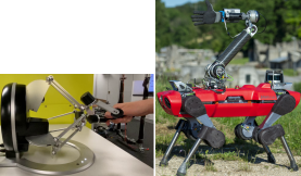
Figure 1: Experimental setup with Omega6 as haptic device at the master side (left) and the ANYmal C platform equipped with a robotic arm at the slave side (right).

For multi-degree of freedom (DOF) floating-base systems, such as quadrupeds or humanoids, optimization-based techniques are prominently adopted for whole-body control (WBC) design [10], [11]. Such control schemes optimize control objectives for multiple tasks, while handling physical constraints, such as actuation limits, friction cone constraints, etc. Passive whole-body controllers have been proposed to compliantly and safely interact with the environment [12], [13]. However, in a haptic teleoperation scenario, existing work has focused on bounding [14] and mapping [15] the operator commands to ensure safe teleoperation and maintain balance, rather than designing a controller that is inherently robust against the effects of time-delays. One way of addressing this problem is through an energy dissipation performed at the output of the whole-body controller, however this could interfere with the constrained optimal solution and render it infeasible. Here, instead of having a control computing layer (transparency layer) and a dissipation layer (passivity layer), we directly create an optimal passivity controller that respects the energy constraints.

Hence, we propose a control framework for the time-delayed haptic teleoperation of a legged robot, that is in particular capable of mitigating the destabilizing effects caused by time delays in the communication link. To this end, we provide new insights for the formulation of energy constraints in optimization-based whole-body controllers. We then validate the effectiveness of our approach with a set of hardware experiments performed on a quadrupedal mobile manipulator, where the robot is teleoperated during end-effector or base control while introducing artificial yet realistic delays in the network. It is worth noting that the resulting architecture is not specific for quadrupedal robots, but is general enough to be applied to any floating-base system, such as humanoids or wheeled robots.

II BILATERAL TELEOPERATION PROBLEM

In this section, we first provide some necessary background on passivity theory. Afterwards, we describe the considered bilateral teleoperator, and how the passivity requirements can be satisfied with the use of energy tanks.

II-A Background on passivity theory

Consider a state-space system given by:

$$\begin{split}\bm{\mathrm{\dot{x}}}&=\bm{\mathrm{f}}(\bm{\mathrm{x}},\bm{\mathrm{u}})\\ \bm{\mathrm{y}}&=\bm{\mathrm{h}}(\bm{\mathrm{x}},\bm{\mathrm{u}}),\\ \end{split}$$ (1)

where $\bm{\mathrm{x}}\in\mathcal{X}\subseteq\mathbb{R}^{n_{x}}$, $\bm{\mathrm{u}}\in\mathcal{U}\subseteq\mathbb{R}^{n_{u}}$, $\bm{\mathrm{y}}\in\mathcal{Y}\subseteq\mathbb{R}^{n_{y}}$.

Definition II.1 ([16])

System (1) is said to be passive with respect to the input $\bm{\mathrm{u}}$ and output $\bm{\mathrm{y}}$ if there exists a continuous function, $\mathcal{H}(\cdot)\geq 0$, called storage function, such that

$$\mathcal{H}(t)-\mathcal{H}(0)\leq\int_{0}^{t}\bm{\mathrm{u}}^{T}(s)\bm{\mathrm{y}}(s)\;ds,$$ (2)

$\forall\mbox{ }t\geq 0$, for all input signals $u\in\mathcal{U}\subseteq\mathbb{R}^{n_{u}}$, for all initial states $x(0)\in\mathcal{X}$ and $n_{u}=n_{y}$.

Equivalently, we can define system (1) to be passive if $\exists\mathcal{H}(\cdot)\geq 0$ such that $\dot{\mathcal{H}}(t)\leq\bm{\mathrm{u}}^{T}(t)\bm{\mathrm{y}}(t)$.

Theorem II.1 ([17])

Consider the two systems

$$\Sigma_{i}:\begin{cases}\bm{\mathrm{\dot{x}}}_{i}=\bm{\mathrm{f}}_{i}(\bm{\mathrm{x}}_{i},\bm{\mathrm{u}}_{i})\\ \bm{\mathrm{y}}_{i}=\bm{\mathrm{h}}_{i}(\bm{\mathrm{x}}_{i},\bm{\mathrm{u}}_{i}),\end{cases}$$ (3)

where $i=1,2$, $n_{u}=n_{y}$, interconnected with the following power-preserving feedback interconnection:

$$\begin{bmatrix}\bm{\mathrm{u}}_{1}\\ \bm{\mathrm{u}}_{2}\\ \end{bmatrix}=\begin{bmatrix}\bm{\mathrm{0}}_{n_{u}\times n_{u}}&\mathcal{\bm{\mathrm{W}}}\\ -\mathcal{\bm{\mathrm{W}}}&\bm{\mathrm{0}}_{n_{u}\times n_{u}}\end{bmatrix}\begin{bmatrix}\bm{\mathrm{y}}_{1}\\ \bm{\mathrm{y}}_{2},\\ \end{bmatrix}$$ (4)

where $\mathcal{\bm{\mathrm{W}}}:=diag(w_{1},...,w_{{n}_{u}})$, $\mathcal{\bm{\mathrm{W}}}\succcurlyeq 0$. If $\Sigma_{i}$ is passive with respect to the mapping $\bm{\mathrm{u}}_{i}\to\bm{\mathrm{y}}_{i}$ with storage function $\mathcal{H}_{\Sigma_{i}}$ for $i=1,2$, then the interconnected system $\Sigma_{1}\wedge\Sigma_{2}$ is also passive and the overall storage function is such that

$$\begin{cases}\mathcal{H}_{\Sigma_{1}\wedge\Sigma_{2}}=\mathcal{H}_{\Sigma_{1}}+\mathcal{H}_{\Sigma_{2}}\\ \dot{\mathcal{H}}_{\Sigma_{1}\wedge\Sigma_{2}}=0.\end{cases}$$ (5)

II-B Control by interconnection

The closed-loop system in Fig. 2 is passive if its interacting components satisfy (2), and are interconnected according to (4). Being mechanical systems, the master and slave are passive, as it can be deduced considering the system Hamiltonian as a storage function. Therefore, a passive control unit needs to be designed to convey energy between the haptic interface and the remote robot.

Figure 2: Diagram of main elements interacting, from left to right: the human operator and the haptic device, the bilateral teleoperator, the slave and the environment.

This can be done by ensuring that the assumptions of Theorem (II.1) are satisfied, i.e. that the passivity requirement (2) holds for the bilateral teleoperator and this results passively interconnected to the master and slave devices. In the next section, we show how to preserve the passivity requirements using the concept of virtual energy tanks [18].

II-C Passivity control with energy tanks

Energy tanks are dynamical systems that are connected to the master and slave systems and exchange energy between each other. The energy stored inside each tank is equal to the one transferred from the other tank, and exchanged with the physical world, and represents the energy budget that can be used to generate desired active behaviours. We denote these two storage elements as: $\Sigma_{mt}(u_{mt},y_{mt})$ and $\Sigma_{st}(u_{st},y_{st})$. The energy tanks are modeled as dynamical systems with the following dynamics:

$$\Sigma_{mt} :\begin{cases}\dot{x}_{mt}=u_{mt}+\left(\frac{P_{mt}^{+}-P_{mt}^{-}}{x_{mt}}\right)\\ y_{mt}=\partial_{x_{mt}}{\mathcal{H}}_{mt}=x_{mt}\end{cases}$$ (6a)

$$\Sigma_{st} :\begin{cases}\dot{x}_{st}=u_{st}+\left(\frac{P_{st}^{+}-P_{st}^{-}}{x_{st}}\right)\\ y_{st}=\partial_{x_{st}}{\mathcal{H}}_{st}=x_{st},\end{cases}$$ (6b)

where $\mathcal{H}_{mt}=\frac{1}{2}{x_{mt}}^{2}$, $\mathcal{H}_{st}=\frac{1}{2}{x_{st}}^{2}$ are the tanks storage functions, and $P^{+}\geq 0$ and $P^{-}\geq 0$ indicate the incoming and outgoing power exchanged between the two tanks. In this work, energy is exchanged only if present inside the tank, according to the energy transfer protocol described in [5]. The systems $\Sigma_{mt}$ and $\Sigma_{st}$ are connected to the master and slave ports, respectively, as follows:

$$\begin{bmatrix}\bm{\mathrm{u}}_{mc}\\ u_{mt}\\ \bm{\mathrm{u}}_{sc}\\ u_{st}\end{bmatrix}=\begin{bmatrix}\leavevmode\hbox to6.67pt{\vbox to6.67pt{\text{[drawing]}}}\bm{\mathrm{0}}&\frac{\bm{\mathrm{w}}_{m}}{x_{mt}}&\bm{\mathrm{0}}&0\\ -\frac{\bm{\mathrm{w}}_{m}^{T}}{x_{mt}}&0\leavevmode\hbox to6.67pt{\vbox to6.67pt{\text{[drawing]}}}&\bm{\mathrm{0}}&0\\ \bm{\mathrm{0}}&0&\leavevmode\hbox to6.67pt{\vbox to6.67pt{\text{[drawing]}}}\bm{\mathrm{0}}&\frac{\bm{\mathrm{w}}_{s}}{x_{st}}\\ \bm{\mathrm{0}}&0&-\frac{\bm{\mathrm{w}}_{s}^{T}}{x_{st}}&0\leavevmode\hbox to6.67pt{\vbox to6.67pt{\text{[drawing]}}}\\ \end{bmatrix}\begin{bmatrix}\bm{\mathrm{y}}_{m}\\ y_{mt}\\ \bm{\mathrm{y}}_{s}\\ y_{st}\end{bmatrix}\leavevmode\hbox to31.26pt{\vbox to33.25pt{\text{[drawing]}}}\leavevmode\hbox to53.59pt{\vbox to27.4pt{\text{[drawing]}}},\\ \bm{\mathrm{D}}_{m} \bm{\mathrm{D}}_{s} \bm{\mathrm{D}}_{m} \bm{\mathrm{D}}_{s}$$ (7)

where $\bm{\mathrm{w}}_{m}\in\mathbb{R}^{n_{y_{m}}}$ and $\bm{\mathrm{w}}_{s}\in\mathbb{R}^{n_{y_{s}}}$ are steer values computed by the master and slave controllers, based on the states of the two tanks ${x_{mt}\text{ and }x_{st}}$. The matrices $\bm{\mathrm{D}}_{m}$ and $\bm{\mathrm{D}}_{s}$ that interconnect the tanks to the respective systems, are in the form of Eq. 4. The resulting bilateral teleoperator energy rate matches the power flowing from master and slave devices into the master and slave controllers, indeed

$$\dot{\mathcal{H}}_{mt}+\dot{\mathcal{H}}_{c}+\dot{\mathcal{H}}_{st}=-\bm{\mathrm{u}}_{mc}^{T}\bm{\mathrm{y}}_{m}-\bm{\mathrm{u}}_{sc}^{T}\bm{\mathrm{y}}_{s}.$$ (8)

where $\dot{\mathcal{H}}_{c}=P_{mt}^{-}-P_{mt}^{+}+P_{st}^{-}-P_{st}^{+}$ is the energy stored in the communication channel. Therefore, the bilateral teleoperator is passive with respect to input $(-\bm{\mathrm{u}}_{mc},-\bm{\mathrm{u}}_{sc})$ and output $(\bm{\mathrm{y}}_{m},\bm{\mathrm{y}}_{s})$. However, if the energy tanks are depleted, there is no possibility to passively implement the desired action. Therefore, the only requirement that we need to impose to preserve the passivity of the system is that the energy level inside each tank is positive. In the next section, we will show how we impose this requirement in the master and slave controllers.

III HYBRID TELEOPERATION CONTROL

In the following sections we provide the implementation details of the proposed setup. First, we introduce the model of the slave, which is described by the equations of motion of a multi-limbed floating-base system:

$$\begin{split}\bm{\mathrm{M}}_{u}(\bm{\mathrm{q}})\dot{\bm{\mathrm{v}}}+\bm{\mathrm{b}}_{u}(\bm{\mathrm{q}},\bm{\mathrm{v}})&=\bm{\mathrm{J}}_{c_{u}}^{T}(\bm{\mathrm{q}})\bm{\mathrm{\lambda}}\\ \bm{\mathrm{M}}_{a}(\bm{\mathrm{q}})\dot{\bm{\mathrm{v}}}+\bm{\mathrm{b}}_{a}(\bm{\mathrm{q}},\bm{\mathrm{v}})&=\bm{\mathrm{J}}_{c_{a}}^{T}(\bm{\mathrm{q}})\bm{\mathrm{\lambda}}+\bm{\mathrm{u}}_{sc},\end{split}$$ (9)

where $\bm{\mathrm{q}}\in SE(3)\times\mathbb{R}^{n_{a}}$ and $\bm{\mathrm{v}}\in\mathbb{R}^{6+n_{a}}$ are the robot generalized coordinates and velocities, $\bm{\mathrm{M}}$ is the mass matrix, $\bm{\mathrm{b}}$ includes the nonlinear effects (i.e. Coriolis, centrifugal, and gravitational terms), and $\bm{\mathrm{u}}_{sc}$ is the vector of actuation torques. Additionally, $\bm{\mathrm{J}}_{c}$ is a matrix of stacked contact Jacobians, while $\bm{\mathrm{\lambda}}$ is the vector of contact wrenches. The subscripts $u$ and $a$ correspond to the unactuated and actuated parts of the defined quantities, respectively. We formulate the slave whole-body control problem as in [11], where a hierarchical QP is solved to determine the vector of desired generalized accelerations ($\dot{\bm{\mathrm{v}}}^{*}$), and desired contact forces $(\bm{\mathrm{\lambda}}^{*})$. We denote the vector of optimization variables with ${\bm{\mathrm{\xi}}=({\dot{\bm{\mathrm{v}}}^{*}},{\bm{\mathrm{\lambda}}^{*}})}$. A set of equality tasks encode dynamic consistency, no slipping or separation of stance legs, as well as tracking of base and limb motion references. Additionally, a set of inequalities is defined to encode friction cone constraints, joint torque limits, in addition to the passivity conditions. The priorities of each task are reported in Table I and will be discussed later in this section. It is worth mentioning that the reference commands from the master device are not directly sent to the whole-body controller, but are given as inputs to an intermediate motion planner [19]. Briefly, this planner solves a model predictive control (MPC) problem to generate optimal motion references for the robot’s base and limbs. These references are then tracked by the passivity-preserving QP hierarchical controller. Given the optimal solution $\bm{\mathrm{\xi}}$ of the WBC, the joint torques are computed by inverting the desired dynamics:

$$\bm{\mathrm{u}}_{sc}=[\bm{\mathrm{M}}_{a}(\bm{\mathrm{q}})\hskip 5.69046pt-\bm{\mathrm{J}}_{c_{a}}^{T}(\bm{\mathrm{q}})]\cdot\bm{\mathrm{\xi}}+\bm{\mathrm{b}}_{a}(\bm{\mathrm{q}},\bm{\mathrm{v}}).$$ (10)

III-A End-effector position control

III-A1 Master controller

Since the controller is implemented on an embedded unit, a discrete-time rule needs to be computed to update the energy tank level [20]:

$$\mathcal{H}_{mt}(k)=\int_{0}^{k\Delta T}\left(u_{mt}+\frac{P_{mt}^{+}-P_{mt}^{-}}{x_{mt}}\right)y_{mt}dt$$

$$=\int_{0}^{k\Delta T}-\bm{\mathrm{w}}_{m}^{T}(t)\bm{\mathrm{y}}_{m}(t)dt+\int_{0}^{k\Delta T}[P^{+}_{mt}(t)-P^{-}_{mt}(t)]dt$$

$$=\sum_{j=1}^{k}-\bm{\mathrm{w}}_{m}^{T}(j-1)\Delta\bm{\mathrm{x}}_{m}(j)+\Delta\mathcal{H}^{+}_{mt}(j)-\Delta\mathcal{H}^{-}_{mt}(j)$$

$$=\mathcal{H}_{mt}(k-1)-\bm{\mathrm{w}}_{m}^{T}(k-1)\Delta\bm{\mathrm{x}}_{m}(k)+\Delta\mathcal{H}_{mt}(k),$$ (11)

with ${\Delta\bm{\mathrm{x}}_{m}(k)=\bm{\mathrm{x}}_{m}(k)-\bm{\mathrm{x}}_{m}(k-1)}$, ${\bm{\mathrm{y}}_{m}=\dot{\bm{\mathrm{x}}}_{m}}$, and ${\Delta\mathcal{H}_{mt}(k)}$ is the overall exchanged energy at time $k$. Let $\bm{\mathrm{F}}_{c}$ be the desired haptic feedback, which is updated based on feedback information from the slave’s end-effector. We compute the master-side steer value $\bm{\mathrm{w}}_{m}$ as a function of both the state of the tank and the desired haptic feedback:

$$\bm{\mathrm{w}}_{m}(k)=\begin{cases}\bm{\mathrm{F}}_{c}(k)&\text{if }\mathcal{H}_{mt}(k)\geq\zeta\\ \frac{x_{mt}^{2}(k)}{\gamma^{2}}\bm{\mathrm{F}}_{c}(k)-\bm{\mathrm{\Gamma}}\cdot{\dot{\bm{\mathrm{x}}}}_{m}&\text{if }0<\mathcal{H}_{mt}(k)<\zeta\end{cases}$$ (12)

where $\zeta>0$ is the minimum energy level in the tank introduced to avoid singularities in the solution, ${\gamma=\sqrt{2\cdot\zeta}}$, and $\bm{\mathrm{\Gamma}}\succ 0$ is a diagonal matrix whose entries are equal to ${\alpha\cdot(\zeta-\mathcal{H}_{mt}(k))}$ with $\alpha>0$. When the value of the tank decreases below this threshold, $\bm{\mathrm{F}}_{c}$ is modulated according to the state of the tank and, additionally, a dissipative term is added to extract energy from the master. The type of modulation proposed here offers the advantage of being smooth, and does not strictly require any estimate of the velocity at the next sample. Generally, up until the next sample is available, there is no way to act on a loss of passivity. However, if $\zeta$ is chosen as the maximum allowable energy to spend, this problem is avoided.

TABLE I: List of tasks used in the WBC. Each task is assigned a priority. The tasks introduced in this work are highlighted, with reference to the corresponding equations.

Priority	Task
1	Equations of motion
	Torque limits
	Friction cone
	Zero acceleration at the contact
2	Base motion direction (21)
	Arm motion direction (18)
3	Base passivity constraint (20)
	Arm passivity constraint (15)
	Base motion tracking
	Limbs motion tracking

III-A2 Slave controller

At the slave side, a similar update for the tank can be obtained as follows:

$$\begin{split}&\mathcal{H}_{st}(k)=\mathcal{H}_{st}(k-1)-{\bm{\mathrm{w}}_{s}}^{T}(k-1)\Delta\bm{\mathrm{q}}_{s}(k)+\Delta\mathcal{H}_{st}(k).\end{split}$$ (13)

At each sample, $\mathcal{H}_{st}$ is updated with the previously applied torques $\bm{\mathrm{w}}_{s}(k-1)=\bm{\mathrm{u}}_{sc}(k-1)$, the joint displacement $\Delta\bm{\mathrm{q}}_{s}(k)=\bm{\mathrm{q}}(k)-\bm{\mathrm{q}}(k-1)$, and the exchange with the master tank $\Delta\mathcal{H}_{st}(k)=\Delta\mathcal{H}_{st}^{+}(k)-\Delta\mathcal{H}_{st}^{-}(k)$. The control law (10) needs to impose that the energy level inside the tank at each instant of time is larger than zero. Since the energy exchange with the master tank $\Delta\mathcal{H}_{st}$ at sample $k+1$ is unknown, we impose the following inequality constraint:

$$\mathcal{\hat{H}}_{st}(k+1)=\mathcal{H}_{st}(k)-\bm{\mathrm{u}}_{sc}^{T}(k)\dot{\bm{\mathrm{q}}}(k)\Delta T\mbox{ }\geq\epsilon,$$ (14)

where $\mathcal{\hat{H}}_{st}$ is an estimate of the tank level at time $k+1$, $\epsilon>0$ is a threshold for the minimum possible energy level, and the joint displacements $\Delta\bm{\mathrm{q}}_{s}(k+1)$ are estimated from the current joint velocities.

During teleoperation of the arm end-effector, we tolerate small variations of the torso, resulting in (14) being mainly affected by the joints of the arm. Under this consideration, Eq. 14 can be rewritten taking (10) into account, as:

$$\small\begin{bmatrix}\dot{\bm{\mathrm{q}}}_{r}^{T}\bm{\mathrm{M}}_{r}&-\dot{\bm{\mathrm{q}}}_{r}^{T}\bm{\mathrm{J}}^{T}_{{c_{r}}}\end{bmatrix}\bm{\mathrm{\xi}}\leq\frac{\mathcal{H}_{st}(k)-\epsilon}{\Delta T}-\dot{\bm{\mathrm{q}}}_{r}^{T}(\bm{\mathrm{b}}_{r}-\bm{\mathrm{g}}_{r})$$ (15)

where the subscript $r$ corresponds to the arm degrees of freedom, $\bm{\mathrm{M}}_{r}$ includes the last $n_{r}$ rows of $\bm{\mathrm{M}}_{a}$, and $\bm{\mathrm{g}}_{r}$ are the arm gravitational torques. These can be subtracted from the energy budget since such a compensation preserves passivity.

Let $\bm{\mathrm{q}}^{*}_{r}$ and $\dot{\bm{\mathrm{q}}}^{*}_{r}$ be the arm joint references computed by the MPC planner. A desired acceleration is generated with a PD control law:

$$\ddot{\bm{\mathrm{q}}}_{r}^{des}=\bm{\mathrm{K}}_{p}(\bm{\mathrm{q}}_{r}^{*}-\bm{\mathrm{q}}_{r})+\bm{\mathrm{K}}_{d}(\dot{\bm{\mathrm{q}}}_{r}^{*}-\dot{\bm{\mathrm{q}}}_{r}).$$ (16)

An equality task is then formulated to track the resulting desired acceleration

$$[\bm{\mathrm{O}}_{n_{r}\times n_{z}}\mbox{ }\mbox{ }\bm{\mathrm{\mathbb{I}}}_{n_{r}\times n_{r}}\mbox{ }\mbox{ }\bm{\mathrm{O}}_{n_{r}\times n_{\lambda}}]\cdot\bm{\mathrm{\xi}}=\ddot{\bm{\mathrm{q}}}_{r}^{des},$$ (17)

where $n_{z}=n_{a}+6-n_{r}$. To avoid having the passivity task invert the direction of the desired accelerations, we impose an additional constraint on the arm’s motion, given by:

$$[\bm{\mathrm{O}}_{n_{r}\times n_{z}}\mbox{ }\mbox{ }\bm{\mathrm{Q}}_{r}\mbox{ }\mbox{ }\bm{\mathrm{O}}_{n_{r}\times n_{\lambda}}]\cdot\bm{\mathrm{\xi}}\geq\bm{\mathrm{0}},$$ (18)

where $\bm{\mathrm{Q}}_{r}\in\mathbb{R}^{n_{r}\times n_{r}}$ is a diagonal matrix with diagonal entries equal to the desired joint accelerations as in (16). A higher priority (see Table I) is assigned to (18) when compared to the passivity and tracking tasks. In this way we ensure that the desired joint-space motion direction is preserved, while jointly optimizing for passivity and transparency (i.e tracking) with a lower priority. One could expect that the passivity task should be at the highest priority. However, as pointed out in [21], since passivity is only sufficient for stability, strictly enforcing passivity could lead to an overly conservative behavior. Hence, for our control architecture, enforcing stability at a lower priority allows to respect the stability requirements, while still guaranteeing a good tracking performance.

III-B Base velocity control

III-B1 Master controller

The base velocity teleoperation problem is challenging since the haptic device has a limited workspace. Ideally, it would be desirable to map master positions to slave velocity commands. However, the master device is passive with respect to the power port $(\bm{\mathrm{u}}_{mc},\dot{\bm{\mathrm{x}}}_{m})$ rather then $(\bm{\mathrm{u}}_{mc},\bm{\mathrm{x}}_{m})$. As in [22], we overcome this issue by rendering the master passive with respect to the port $(\bm{\mathrm{u}}_{mc},\bm{\mathrm{r}}_{m})$, where the output $\bm{\mathrm{r}}_{m}$ is defined as: ${\bm{\mathrm{r}}_{m}=\dot{\bm{\mathrm{x}}}_{m}+\bm{\mathrm{\Lambda}}\bm{\mathrm{x}}_{m}}$, with ${\bm{\mathrm{\Lambda}}\succ 0}$; and a local control action is added to $\bm{\mathrm{u}}_{mc}$ as $-\bm{\mathrm{B}}\dot{\bm{\mathrm{x}}}_{m}-\bm{\mathrm{K}}\bm{\mathrm{x}}_{m}$. The matrix $\bm{\mathrm{B}}$ is chosen such that $\bm{\mathrm{B}}\succ\bm{\mathrm{M}}_{m}\bm{\mathrm{\Lambda}}$, with $\bm{\mathrm{M}}_{m}$ being the mass matrix of the haptic device, $\bm{\mathrm{K}}\succ 0$. As shown in [23], the signal $\bm{\mathrm{r}}_{m}$ can be made proportional only to the scaled position if the contribution of velocity is negligible due to the choice of $\bm{\mathrm{\Lambda}}$.

III-B2 Slave controller

The slave degrees of freedom controlled in velocity mode are the lateral and longitudinal velocities of the base. No references are sent along the vertical direction, however we still allow for feedback. In this way, if the base of the robot is disturbed along this direction, the operator could still perceive the applied force. Since the floating-base of a legged robot is driven by generating contact forces on the environment, we impose the energetic limitation with respect to the $xy$ (non-vertical) forces exerted by the stance legs:

$$\mathcal{\hat{H}}_{st}(k+1)=\mathcal{H}_{st}(k)-(\bm{\mathrm{J}}^{T}_{{u}_{xy}}\bm{\mathrm{\lambda}})^{T}\dot{\bm{\mathrm{x}}}_{s_{xy}}\Delta T\geq\epsilon,$$ (19)

where $\bm{\mathrm{J}}^{T}_{u_{xy}}$ includes the first two rows of ($\bm{\mathrm{J}}_{c_{u}}^{T}$), and $\dot{\bm{\mathrm{x}}}_{s}$ is the base velocity. Using (9), we can rewrite (19) as:

$$\small[\bm{\mathrm{\dot{x}}}_{s_{xy}}^{T}\bm{\mathrm{M}}_{xy}\;\;\;\bm{\mathrm{0}}_{2\times n_{\lambda}}]\cdot\bm{\mathrm{\xi}}\leq\frac{\mathcal{H}_{st}(k)-\epsilon}{\Delta T}\;-\dot{\bm{\mathrm{x}}}_{s_{xy}}^{T}(\bm{\mathrm{b}}_{xy}-\bm{\mathrm{g}}_{xy}),$$ (20)

which can be added as a task in the hierarchical QP. As in Sec. III-A, the desired linear accelerations calculated by the motion planner should be preserved. These accelerations are expressed in a specific frame, named control frame $C$ [11], which changes according to the slope of the terrain and the base orientation. To prevent changes in desired references, we add the following additional inequality constraint to the stack of tasks:

$$\begin{bmatrix}\bm{\mathrm{Q}}_{xy}\bm{\mathrm{J}}_{u_{xy}}&\bm{\mathrm{0}}_{2\times n_{\lambda}}\end{bmatrix}\cdot\bm{\mathrm{\bm{\mathrm{\xi}}}}+\bm{\mathrm{Q}}_{xy}\dot{\bm{\mathrm{J}}}_{u_{xy}}\bm{\mathrm{v}}\geq\bm{\mathrm{0}},$$ (21)

where $\bm{\mathrm{Q}}_{xy}\in\mathbb{R}^{2\times 2}$ is a diagonal matrix with entries equal to the elements of the desired linear acceleration ${}_{C}\ddot{\bm{\mathrm{r}}}^{des}_{xy}$, which is computed as follows:

$${}_{C}\ddot{\bm{\mathrm{r}}}^{des}_{xy}={}_{C}\ddot{\bm{\mathrm{r}}}_{xy}^{*}+\bm{\mathrm{K}}_{d}({}_{C}\dot{\bm{\mathrm{r}}}_{xy}^{*}-{}_{C}\dot{\bm{\mathrm{r}}}_{xy})+\bm{\mathrm{K}}_{p}({}_{C}{\bm{\mathrm{r}}}_{xy}^{*}-{}_{C}{\bm{\mathrm{r}}}_{xy}).\\$$ (22)

IV EXPERIMENTAL RESULTS

We validated our proposed teleoperation framework through experiments performed on a real robot platform with an artificial delay introduced in the network. Videos of all the experiments are available in the attached multimedia material. The master device used for the experiments is the Force Dimension Omega.6 haptic device. The slave robot is ANYmal – a torque-controlled quadrupedal robot – equipped with a 4 DOF robotic arm. The control loop runs at 1 kHz on the haptic device, while the ANYmal whole-body controller and the state estimator run at 400 Hz on the robot’s onboard computer (Intel Corei7-8850H CPU@4GHz hexacore processor). Each experiment is performed without and with the proposed passivity framework. We provide results for end-effector position control and base velocity control, with an end-to-end added delay of 60 ms for the two scenarios. This delay was observed as the average communication delay between the University of Twente and our laboratory in Zurich.

IV-A End-effector position control

In this experiment, the human operator moves the haptic device along a predefined trajectory, defined in such a way to span the whole workspace up to the boundaries of the haptic device.

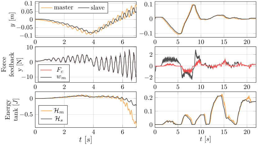
Figure 3: Master and slave end-effector position, force and energy tanks levels with passivity layer (right), and without (left), during an experiment of end-effector control.

For this experiment, the local force feedback used in Eq. (12) was generated from the displacement error between the master and the slave measured position: $\bm{\mathrm{F}}_{c}(k)=\bm{\mathrm{K}}_{p}(\bm{\mathrm{x}}_{s}(k-k_{d})-\bm{\mathrm{x}}_{m}(k))$ where $k_{d}$ is the time delay. Results for this experiment are displayed in Fig. 3 where, for the sake of conciseness, only the plots along the y direction are reported. It can be seen that, without the passivity layer, the two devices show oscillatory signals that are out-of-phase. In this condition, to avoid damages to the hardware, the system is frozen as soon as the oscillations start to grow. Another indicator of unstable behavior is observed in the plot of the energy tank level, where a drop to a negative value occurs. Conversely, with passivity layer, this behavior is avoided and leads to smoother master and slave trajectories.

IV-B Base velocity control

In this experiment, we control the base velocity of the slave. To avoid hardware damage we limit the maximum commanded velocity to 0.2 m/s. For this test, the local force feedback used in Eq. 12 was generated from the velocity tracking error at the slave side: ${\bm{\mathrm{F}}_{c}(k)=\bm{\mathrm{K}}_{v}(\bm{\mathrm{v}}_{m}(k-k_{d})-\bm{\mathrm{v}}_{s}(k))}$, where $\bm{\mathrm{v}}_{m}$, and $\bm{\mathrm{v}}_{s}$ denote the master velocity, and the slave base velocity, respectively. $\bm{\mathrm{v}}_{m}$ is computed from the master position using the mapping from Section III-B. This haptic feedback allows to realistically perceive external forces, and to capture their effect without the need for any haptic sensory feedback.

Figure 4: Master and slave $x$-$y$ velocity profiles with passivity layer (right), and without (left) in base velocity control.

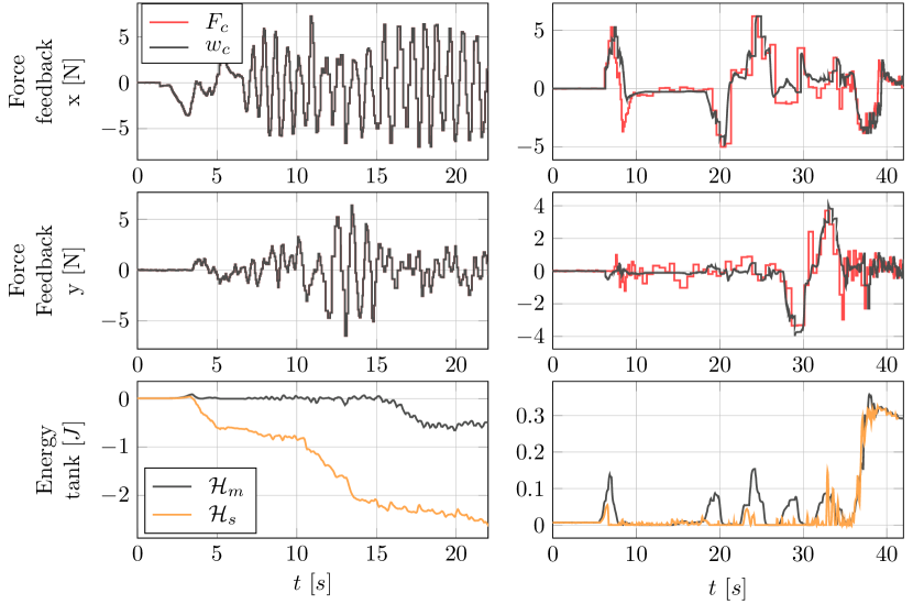
Figure 5: Force and energy tanks levels with passivity layer (right), and without (left) in base velocity control.

It can be noted from Fig. 4 that, with passivity layer, the velocity tracking error increases as the master velocity is about to reach $0.2\ \text{m/s}$. While the master velocity is about reaching this peak, the mean absolute percentage tracking error in velocity is 6.98% without passivity layer, and only 1.1% with passivity layer. The former scenario happens in order to avoid violating the passivity condition as seen in the energy level plots of Fig. 5, which in turn leads to the energetic penalization of the contact forces along the directions where they create motion. As shown in Fig. 4, if passivity is not enforced, the force feedback causes the haptic device to become unstable, and this in turn compromises tracking. Enforcing passivity allows to avoid this problem and results in a stable teleoperation system.

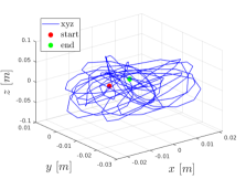
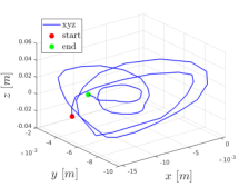
Figure 6: 3D position trajectories for the slave end-effector during two experiments of haptic interaction with a human, with energy tanks off (left), and on (right).

IV-C Haptic interaction during end-effector control

In this experiment, we perform a haptic interaction test with a human at the slave side shaking the robot’s hand. Haptic feedback was generated as in Sec. IV-A. For the sake of conciseness, we only present results for the slave response (Fig. 6). From both the plots and the video attachment, it can be verified that, with passivity, the trajectories are smoother and the system remains stable. Gains for the master controller were tuned in such a way that enables the operator to perceive low magnitude forces acting on the slave end-effector. We realized that, if it is desired that the operator feels the hand-shake, these gains tend to be high, leading to a more unstable behavior. Indeed, in haptic teleoperation, instabilities are due not only to time delays, but also to other sources, such as those deriving from a controller tuning that aims to enhance transparency. However, it can be noted from Fig. 6 that our formulation is also effective in handling this additional source of instability.

V CONCLUSIONS

In this paper, we presented an approach to ensure the stability of a haptic teleoperation system for a quadrupedal mobile manipulator. The crucial point to ensure such a property is to manage a potential active behavior of the bilateral teleoperator. We addressed such a problem for the bilateral teleoperation of a general floating-base system, in the presence of destabilizing time delays. To this end, energy tanks were used as energy observers and included in the formulation of a passive QP controller at the slave side. We experimentally demonstrated that, in the presence of time delays, the proposed passivity formulation based on energy tanks effectively leads to more stable operations. One interesting direction for future work includes adding feedback from force sensor measurements, and extending the proposed method to perform tele-manipulation tasks, such as remotely turning valves or opening doors.

References

• [1] J. G. Wildenbeest, D. A. Abbink, C. J. Heemskerk, F. C. Van Der Helm, and H. Boessenkool, “The impact of haptic feedback quality on the performance of teleoperated assembly tasks,” IEEE Transactions on Haptics, vol. 6, no. 2, pp. 242–252, 2012.
• [2] R. J. Anderson and M. W. Spong, “Bilateral control of teleoperators with time delay,” in IEEE International Conference on Systems, Man, and Cybernetics, vol. 1.   IEEE, 1988, pp. 131–138.
• [3] P. F. Hokayem and M. W. Spong, “Bilateral teleoperation: An historical survey,” Automatica, vol. 42, no. 12, pp. 2035–2057, 2006.
• [4] R. Muradore and P. Fiorini, “A review of bilateral teleoperation algorithms,” Acta Polytechnica, vol. 13, no. 1, pp. 191–208, 2016.
• [5] M. Franken, S. Stramigioli, S. Misra, C. Secchi, and A. Macchelli, “Bilateral telemanipulation with time delays: A two-layer approach combining passivity and transparency,” IEEE transactions on robotics, vol. 27, no. 4, pp. 741–756, 2011.
• [6] G. Niemeyer and J.-J. Slotine, “Stable adaptive teleoperation,” IEEE Journal of oceanic engineering, vol. 16, no. 1, pp. 152–162, 1991.
• [7] J.-H. Ryu, D.-S. Kwon, and B. Hannaford, “Stable teleoperation with time-domain passivity control,” IEEE Transactions on robotics and automation, vol. 20, no. 2, pp. 365–373, 2004.
• [8] E. Sartori, C. Tadiello, C. Secchi, and R. Muradore, “Tele-echography using a two-layer teleoperation algorithm with energy scaling,” in International Conference on Robotics and Automation, ICRA, Montreal, QC, Canada.   IEEE, 2019, pp. 1569–1575.
• [9] O. A. M. Franco, J. Bimbo, C. Pacchierotti, D. Prattichizzo, D. Barcelli, and G. Bianchini, “Transparency-optimal passivity layer design for time-domain control of multi-dof haptic-enabled teleoperation,” in 2018 IEEE/RSJ International Conference on Intelligent Robots and Systems (IROS).   IEEE, 2018, pp. 4988–4994.
• [10] L. Sentis and O. Khatib, “Synthesis of whole-body behaviors through hierarchical control of behavioral primitives,” International Journal of Humanoid Robotics, vol. 2, no. 04, pp. 505–518, 2005.
• [11] C. D. Bellicoso, C. Gehring, J. Hwangbo, P. Fankhauser, and M. Hutter, “Perception-less terrain adaptation through whole body control and hierarchical optimization,” in IEEE-RAS 16th International Conference on Humanoid Robots (Humanoids).   IEEE, 2016, pp. 558–564.
• [12] S. Fahmi, C. Mastalli, M. Focchi, and C. Semini, “Passive whole-body control for quadruped robots: Experimental validation over challenging terrain,” IEEE Robotics and Automation Letters, vol. 4, no. 3, pp. 2553–2560, 2019.
• [13] B. Henze, M. A. Roa, and C. Ott, “Passivity-based whole-body balancing for torque-controlled humanoid robots in multi-contact scenarios,” The International Journal of Robotics Research, vol. 35, no. 12, pp. 1522–1543, 2016.
• [14] G. Xin, J. Smith, D. Rytz, W. Wolfslag, H.-C. Lin, and M. Mistry, “Bounded haptic teleoperation of a quadruped robot’s foot posture for sensing and manipulation,” in 2020 IEEE International Conference on Robotics and Automation (ICRA).   IEEE, 2020, pp. 1431–1437.
• [15] W. Gomes, V. Radhakrishnan, L. Penco, V. Modugno, J. Mouret, and S. Ivaldi, “Humanoid whole-body movement optimization from retargeted human motions,” in 19th IEEE-RAS International Conference on Humanoid Robots, Humanoids 2019, Toronto, ON, Canada, October 15-17, 2019.   IEEE, 2019, pp. 178–185.
• [16] T. Gilead, L. Rogelio, B. Bernard, E. Olav, and M. Bernhard, “Dissipative systems analysis and control,” Autom., vol. 41, no. 1, pp. 177–179, 2005.
• [17] C. Ebenbauer, T. Raff, and F. Allgöwer, “Dissipation inequalities in systems theory: An introduction and recent results,” in Invited lectures of the international congress on industrial and applied mathematics, vol. 2007, 2009, pp. 23–42.
• [18] T. S. Tadele, T. J. De Vries, and S. Stramigioli, “Combining energy and power based safety metrics in controller design for domestic robots,” in IEEE International Conference on Robotics and Automation (ICRA).   IEEE, 2014, pp. 1209–1214.
• [19] J.-P. Sleiman, F. Farshidian, M. V. Minniti, and M. Hutter, “A unified mpc framework for whole-body dynamic locomotion and manipulation,” IEEE Robotics And Automation Letters, 2021.
• [20] S. Stramigioli, C. Secchi, A. J. van der Schaft, and C. Fantuzzi, “Sampled data systems passivity and discrete port-hamiltonian systems,” IEEE Transactions on Robotics, vol. 21, no. 4, pp. 574–587, 2005.
• [21] M. Selvaggio, P. R. Giordano, F. Ficuciellol, and B. Siciliano, “Passive task-prioritized shared-control teleoperation with haptic guidance,” in International Conference on Robotics and Automation (ICRA).   IEEE, 2019, pp. 430–436.
• [22] D. Lee and D. Xu, “Feedback r-passivity of lagrangian systems for mobile robot teleoperation,” in IEEE International Conference on Robotics and Automation.   IEEE, 2011, pp. 2118–2123.
• [23] A. Franchi, C. Secchi, H. I. Son, H. H. Bulthoff, and P. R. Giordano, “Bilateral teleoperation of groups of mobile robots with time-varying topology,” IEEE Transactions on Robotics, vol. 28, no. 5, pp. 1019–1033, 2012.