sectioning fifi ffff

Multidimensional Persistence:
Invariants and Parameterization

Abstract. This article grew out of the theoretical part of my Master’s thesis at the Faculty of Mathematics and Information Science at Ruprecht-Karls-Universität Heidelberg under the supervision of PD Dr. Andreas Ott. Following the work of G. Carlsson and A. Zomorodian on the theory of multidimensional persistence in 2007 and 2009, the main goal of this article is to give a complete classification and parameterization for the algebraic objects corresponding to the homology of a multifiltered simplicial complex. As in the work of G. Carlsson and A. Zomorodian, this classification and parameterization result is then used to show that it is only possible to obtain a discrete and complete invariant for these algebraic objects in the case of one-dimensional persistence, and that it is impossible to obtain the same in dimensions greater than one.

1 Introduction

Persistent homology allows us to analyze topological features of increasing filtrations of topological spaces with a complete and discrete invariant, the so-called (persistence) barcode. Many applications of topology lead to multifiltrations, e.g. if we analyze time dependent point cloud datasets as in [BBC⁺21].

In this article, we investigate the theoretical aspects of multidimensional persistence, the extension of the one dimensional concept of persistent homology. This article is mainly based on the work of G. Carlsson and A. Zomorodian in [CZ07] and [CZ09]. [CZ07] and [CZ09] are very similar where the difference is that [CZ09] digs deeper into the details. Both [CZ07] and [CZ09] contain unproven statements. So, one of our main tasks is to fill in the gaps in [CZ07] and [CZ09]. Following [CZ07] and [CZ09], our main goal is to carry out a complete classification (Section 3) and parameterization (Section 4) of the algebraic objects that correspond to the homology of a multifiltered simplicial complex. As in [CZ07] and [CZ09], we then use the parameterization result to show that it is only possible to obtain a discrete and complete invariant for these algebraic objects in the case of one-dimensional persistence, and that it is impossible to obtain the same in dimension greater than one. Here, a discrete invariant is an invariant which is countable in size and which takes values in the same set independently of the underlying coefficient field (see 2.21) and a complete invariant is an invariant which is injective as a function on the objects of classification (see 2.19). At the end of Section 3, we discuss a discrete invariant for multidimensional persistence, the so-called rank invariant (introduced in [CZ07] and [CZ09]), which is practicable for analyzing multiparamter problems and equivalent to the barcode in dimension one.

Our approach in Section 3, based on [CZ07, Sec. 4] and [CZ09, Sec. 4], can be summarized as follows: first of all, we have to determine the algebraic objects which correspond to the homology of a finite $n$-filtered simplicial complex (see Section 2.2). As it turns out, any finite $n$-filtered simplicial complex defines a finitely generated $n$-graded $A_{n}^{\mathbb{F}}$-module $M$ where $A_{n}^{\mathbb{F}}=\mathbb{F}[x_{1},\dots,x_{n}]$ (see Sections 2.3 and 3.1). Moreover, if $\mathbb{F}=\mathbb{F}_{p}$ where $p\in\mathbb{N}$ is a prime number or $\mathbb{F}=\mathbb{Q}$, any such module $M$ can be realized as a finite $n$-filtered simplicial complex (see 3.5).

For the following, denote by $\mathbf{Grf}_{n}(A_{n}^{\mathbb{F}})$ the category of finitely generated $n$-graded $A_{n}^{\mathbb{F}}$-modules together with graded $A_{n}^{\mathbb{F}}$-module homomorphisms as morphisms. In Section 3.2, we show that any $M\in\mathbf{Grf}_{n}(A_{n}^{\mathbb{F}})$ admits a free hull, i.e. there exists a pair $(F,p)$ where ${F\in\mathbf{Grf}_{n}(A_{n}^{\mathbb{F}})}$ is graded free and $p:F\to M$ is a graded surjective $A_{n}^{\mathbb{F}}$-module homomorphism such that

$$\mathrm{id}_{\mathbb{F}}\otimes_{A_{n}^{\mathbb{F}}}p:\mathbb{F}\otimes_{A_{n}^{\mathbb{F}}}F\xlongrightarrow{\sim}\mathbb{F}\otimes_{A_{n}^{\mathbb{F}}}M$$

is a graded isomorphism of $n$-graded $\mathbb{F}$-vector spaces. Here $A_{n}^{\mathbb{F}}$ acts on $\mathbb{F}$ by setting the variable action identical to zero. By using an $n$-graded version of Nakayama’s Lemma (see 3.16), it is possible to show that $(F,p)$ is a free hull of $M$ if and only if $p$ maps a homogeneous $A_{n}^{\mathbb{F}}$-basis of $F$ to a minimal system of homogeneous generators of $M$ (see 3.20).

Every graded free $F\in\mathbf{Grf}_{n}(A_{n}^{\mathbb{F}})$ admits a graded isomorphism

$$F\cong\mathcal{F}_{n}^{\mathbb{F}}(\xi):=\bigoplus_{v\in V}A_{n}^{\mathbb{F}}(v)^{\mu(v)}$$

where

$$\xi=(V,\mu):=\bigcup_{v\in V}\{(v,1),\dots,(v,\mu(v))\}$$

is an $n$-dimensional multiset with $V\subseteq\mathbb{N}^{n}$ and mulitplicity function $\mu:V\to\mathbb{N}_{\geq 1}$ (see 2.2) and $A_{n}^{\mathbb{F}}(v)$ is a polynomial ring shifted upwards in grading by $v$ (see 2.10).

The main theorem on free hulls (see 3.12) states that free hulls are unique up to isomorphism and that every $M\in\mathbf{Grf}_{n}(A_{n}^{\mathbb{F}})$ admits a free hull

$$p:\mathcal{F}^{\mathbb{F}}_{n}(\xi)\longrightarrow M$$

for a finite $n$-dimensional multiset $\xi$. If $(\mathcal{F}_{n}^{\mathbb{F}}(\xi),p)$ is a free hull of $M$, then $\xi$ is also called the type of $M$. If $G\subseteq M$ is a minimal set of homogeneous generators of $M$, the multiset $\xi$ tells us in which degrees the generators in $G$ are located. Free hulls can be viewed as the basic building block of a minimal graded free resolution of $M$ (see 3.25).

Let us denote by

$$\mathbf{Grf}_{n}(A_{n}^{\mathbb{F}})/_{\cong}$$

the set of all isomorphism classes $[M]$ of objects $M\in\mathbf{Grf}_{n}(A_{n}^{\mathbb{F}})$. Indeed, $\mathbf{Grf}_{n}(A_{n}^{\mathbb{F}})/_{\cong}$ is a set (see 3.23). Denote by

$$I_{n}^{\mathbb{F}}(\xi_{0},\xi_{1})\subseteq\mathbf{Grf}_{n}(A_{n}^{\mathbb{F}})/_{\cong}$$

the subset of all $[M]$ such that $M$ admits a free hull $p_{0}:\mathcal{F}_{n}^{\mathbb{F}}(\xi_{0})\to M$ and $\mathrm{ker}(p_{0})$ admits a free hull $p_{1}:\mathcal{F}_{n}^{\mathbb{F}}(\xi_{1})\to\mathrm{ker}(p_{0})$.

Let $L\subseteq\mathcal{F}_{n}^{\mathbb{F}}(\xi_{0})$ be a graded $A_{n}^{\mathbb{F}}$-submodule. We say that $L$ satisfies the tensor-condition (see Section 3.3.2) if the image of the induced morphism

$$\mathbb{F}\otimes_{A_{n}^{\mathbb{F}}}L\longrightarrow\mathbb{F}\otimes_{A_{n}^{\mathbb{F}}}\mathcal{F}_{n}^{\mathbb{F}}(\xi_{0})$$

is zero. Denote by $S_{n}^{\mathbb{F}}(\xi_{0},\xi_{1})$ the set of all graded $A_{n}^{\mathbb{F}}$-submodules $L\subseteq\mathcal{F}_{n}^{\mathbb{F}}(\xi_{0})$ of type $\xi_{1}$ which satisfy the tensor-condition.

As in [CZ09, Sec. 4.5], we obtain a well-defined set theoretic surjection

$$S_{n}^{\mathbb{F}}(\xi_{0},\xi_{1})\longrightarrow I_{n}^{\mathbb{F}}(\xi_{0},\xi_{1}),\quad L\longmapsto[\mathcal{F}_{n}^{\mathbb{F}}(\xi_{0})/L].$$

Without the tensor-condition this map would not be well-defined. In [CZ07] and [CZ09], the tensor-condition is missing. This surjection induces a set theoretic bijection

$$S_{n}^{\mathbb{F}}(\xi_{0},\xi_{1})/{\mathrm{Aut}(\mathcal{F}_{n}^{\mathbb{F}}(\xi_{0}))}\xlongrightarrow{\sim}{I}_{n}^{\mathbb{F}}(\xi_{0},\xi_{1})$$

which provides a complete classification of ${I}_{n}^{\mathbb{F}}(\xi_{0},\xi_{1})$ (see 3.29 and [CZ09, Thm. 9]). Now the question is if there exists a discrete parameterization of

$$S_{n}^{\mathbb{F}}(\xi_{0},\xi_{1})/{\mathrm{Aut}(\mathcal{F}_{n}^{\mathbb{F}}(\xi_{0}))}.$$

In Section 3.6, we approach this question by considering a possible candidate for a discrete and complete invariant for $\mathbf{Grf}_{n}(A_{n}^{\mathbb{F}})/_{\cong}$, the so-called rank invariant (introduced in [CZ07, Sec. 6] and [CZ09, Sec. 6]). In dimension $n=1$, the rank invariant is equivalent to the barcode (see 3.36) and defines hence a complete and discrete invariant (see [CZ07, Thm. 5] and [CZ09, Thm. 12]). So, the rank invariant can be viewed as a discrete generalization of the barcode to dimension $n\geq 2$. But as we will see in Section 4, the rank invariant is not complete in dimension $n\geq 2$.

In Section 4, our first goal is to show that for $n\geq 2$, there exists no discrete and complete invariant for $\mathbf{Grf}_{n}(A_{n}^{\mathbb{F}})/_{\cong}$. For this, we parameterize $S_{n}^{\mathbb{F}}(\xi_{0},\xi_{1})$ as a subset of a product of Grassmannians together with a group action of ${\mathrm{Aut}(\mathcal{F}_{n}^{\mathbb{F}}(\xi_{0}))}$. This approach follows [CZ07, Sec. 5] and [CZ09, Sec. 5] and is carried out in Sections 4.1-4.3. Based on [CZ07, Sec. 5.2] and [CZ09, Sec. 5.2], we then give a counterexample in Section 4.4 showing the non-existence of a discrete and complete invariant for $\mathbf{Grf}_{n}(A_{n}^{\mathbb{F}})/_{\cong}$ if $n\geq 2$: for $n=2$, consider

$$\xi_{0} =\{((0,0),1),((0,0),2)\}$$

$$\xi_{1} =\{((3,0),1),((2,1),1),((1,2),1),((0,3),1)\}.$$

By using the parameterization result (see Theorems 4.2 and 4.22), we see that $S_{2}^{\mathbb{F}}(\xi_{0},\xi_{1})$ is in bijection to a fourfold product of the Grassmannian $\mathrm{G}_{\mathbb{F}}(1,2)$. Note that $\mathrm{G}_{\mathbb{F}}(1,2)$ equals the projective line $\mathbb{P}_{1}(\mathbb{F})$. The automorphism group $\mathrm{Aut}(\mathcal{F}_{2}^{\mathbb{F}}(\xi_{0}))$ is isomorphic to $\mathrm{GL}_{2}(\mathbb{F})$ (see 4.12). Thus, we obtain set theoretic bijections

$$I_{2}^{\mathbb{F}}(\xi_{0},\xi_{1})\cong S_{2}^{\mathbb{F}}(\xi_{0},\xi_{1})/\mathrm{Aut}(\mathcal{F}_{2}^{\mathbb{F}}(\xi_{0}))\cong\mathbb{P}_{1}(\mathbb{F})^{4}/\mathrm{GL}_{2}({\mathbb{F}})$$

and $I_{2}^{\mathbb{F}}(\xi_{0},\xi_{1})\cong\mathbb{P}_{1}(\mathbb{F})^{4}/\mathrm{GL}_{2}({\mathbb{F}})$ is uncountable if $\mathbb{F}$ is uncountable. For $n>2$, we just have to append zeros to the entries of $\xi_{0}$ and $\xi_{1}$.

Based on and inspired by [CZ07, Sec. 5] and [CZ09, Sec. 5], Section 4.5 is devoted to the investigation of goal number two in Section 4: showing that $S_{n}^{\mathbb{F}}(\xi_{0},\xi_{1})$, which we have paramterized as a subset of a product of Grassmannians, corresponds to the set of $\mathbb{F}$-points of an algebraic variety together with an algebraic group action of ${\mathrm{Aut}(\mathcal{F}_{n}^{\mathbb{F}}(\xi_{0}))}$. In other words, we want to give an explicit parameterization of the moduli space of our classification problem.

Acknowledgements. I want to thank my supervisor Andreas Ott for his motivating support and the inspiring discussions about TDA and its current applications to the viral evolution of SARS-CoV-2.

2 Preliminaries

This section introduces the basic definitions and notations required for this article.

2.1 Multisets

This section follows [CZ07] and [CZ09]. We just add some details and definitions. The next definition introduces a partial order on ${\mathbb{N}^{n}}$, where $\mathbb{N}=\{0,1,2,3,\dots\}$ denotes the set of natural numbers.

Definition 2.1 (Partial order).

1. We define a partial order $\preceq$ on ${\mathbb{N}^{n}}$ as follows: let

   $$s=(s_{1},...,s_{n}),t=(t_{1},...,t_{n})\in{\mathbb{N}^{n}}.$$

   We write $s\preceq t$ if and only if $s_{i}\leq t_{i}$ for all $i\in\{1,...,n\}$. We write $s\prec t$ if and only if $s\preceq t$ and $s_{i}<t_{i}$ for some $i\in\{1,\dots,n\}$. If $s\preceq t$ we also write $t\succeq s$ and if $s\prec t$ we also write $t\succ s$.

2. If $n=1$, then $\preceq$ equals the total order $\leq$ on ${\mathbb{N}}$.

3. For $S\subseteq{\mathbb{N}^{n}}$ and $c\in\mathbb{N}^{n}$, define $S_{\succeq c}:=\{z\in S\mid z\succeq c\}$ and ${S_{\succ c}:=\{z\in S\mid z\succ c\}}$.

4. Let $v,w\in{\mathbb{N}^{n}}$. If $\neg(v\succeq w)$ we also write $v\nsucceq w$. This means that $v\in{\mathbb{N}^{n}}\setminus{\mathbb{N}^{n}_{\succeq w}}$. Note that in general, $v\nsucceq w$ does not imply $v\prec w$ (except only if $n=1$). If $\neg(v\succ w)$ we also write $v\nsucc w$. This means that $v\in{\mathbb{N}^{n}}\setminus{\mathbb{N}^{n}_{\succ w}}$. Note that in general, $v\nsucc w$ does not imply that $v\preceq w$ (except only if $n=1$). For $\prec,\preceq$, the symbols $\nprec,\npreceq$ are defined analogously.

Multisets are one of the basic building blocks for the classification of finitely generated $n$-graded $A_{n}^{\mathbb{F}}$-modules. A multiset may be viewed as a set where elements are allowed to appear more than once.

Definition 2.2.

Recall that $\mathbb{N}=\{0,1,2,3,\dots\}$. Let $n\in\mathbb{N}_{\geq 1}$. Let $S\subseteq{\mathbb{N}^{n}}$ and $\mu:S\to\mathbb{N}_{\geq 1}$ be a map. Then

$$(S,\mu):=\bigcup_{s\in S}\{(s,1),\dots,(s,\mu(s))\}\subseteq S\times\mathbb{N}_{\geq 1}$$

is called an $n$-dimensional multiset. The map $\mu:S\to\mathbb{N}_{\geq 1}$ is also called the multiplicity function of $\xi$ and for $s\in S$, $\mu(s)$ is called the multiplicity of $s$. For ${(s,l),(t,k)\in(S,\mu)}$, define $(s,l)\preceq(t,k)$ if and only if $s\preceq t$ and $(s,l)\prec(t,k)$ if and only if $s\prec t$. Again, if $(s,l)\preceq(t,k)$ we also write $(t,k)\succeq(s,l)$ and if $(s,l)\prec(t,k)$ we also write $(t,k)\succ(s,l)$.

Example 2.3.

We present two examples of multisets:

1. Consider the one-dimensional multiset

   $$\xi=\{(1,1),(1,2),(2,1)\}.$$

   We have $\xi=(S,\mu)$ where $S=\{1,2\}\subseteq\mathbb{N}$, $\mu(1)=2$ and $\mu(2)=1$.

2. Consider the two-dimensional multiset

   $$\xi=\{((1,1),1),((1,1),2),((2,2),1)\}.$$

   We have $\xi=(S,\mu)$ where $S=\{(1,1),(2,2)\}\subseteq\mathbb{N}^{2}$, ${\mu(1,1)=2}$ and $\mu(2,2)=1$.

Definition 2.4.

Let $\xi_{0},\xi_{1}$ be two $n$-dimensional multisets. We write $\xi_{1}\succ_{D}\xi_{0}$ if $v\succ w$ for all $v\in\xi_{1}$ and all $w\in\xi_{0}$. In this case, we say that $\xi_{1}$ dominates $\xi_{0}$.

Example 2.5.

Consider

$$\xi_{0} =\{((0,0),1),((0,0),2)\}$$

$$\xi_{1} =\{((1,1),1),((1,1),2),((2,2),1)\}.$$

Then $\xi_{1}\succ_{D}\xi_{0}$.

2.2 Multifiltered simplicial complexes

For the next two definitions, we follow [HOST19, Def. 2.1] (which is compatible with [CZ07] and [CZ09]).

Definition 2.6.

Let $(X_{u})_{u\in{\mathbb{N}^{n}}}$ be a familiy of simplicial complexes (for a definition of simplicial complex see [Mun18, §1-3]).

1. $(X_{u})_{u\in{\mathbb{N}^{n}}}$ is called an $n$-filtration (one-filtration if $n=1$ and bifiltration if $n=2$) if $X_{u}\subseteq X_{v}$ for all $u,v\in{\mathbb{N}^{n}}$ with $u\preceq v$.

2. If $(X_{u})_{u\in{\mathbb{N}^{n}}}$ is an $n$-filtration, then we say that $(X_{u})_{u\in{\mathbb{N}^{n}}}$ stabilizes if there exists a $w\in{\mathbb{N}^{n}}$ such that $X_{u}=X_{w}$ for all $u\in{\mathbb{N}^{n}_{\succeq w}}$.

Definition 2.7.

Let $X$ be a simplicial complex.

1. $X$ is called $n$-filtered if $X=\bigcup_{u\in{\mathbb{N}^{n}}}X_{u}$ for an $n$-filtration of simplicial complexes $(X_{u})_{u\in{\mathbb{N}^{n}}}$ which stabilizes. $X$ is called multifiltered if $X$ is $n$-filtered for some $n\in\mathbb{N}$. We often write $X=(X_{u})_{u\in{\mathbb{N}^{n}}}$ to indicate that $X$ is an $n$-filtered simplicial complex with $X=\bigcup_{u\in{\mathbb{N}^{n}}}X_{u}$.

2. $X$ is called a finite $n$-filtered simplicial complex if $X$ is an $n$-filtered simplicial complex and if $X$ is finite (i.e. the set of vertices of $X$ is finite).

2.3 n-graded rings and modules

This section introduces basic facts and definitions about $n$-graded commutative rings and modules. Our definitions are compatible with [CZ07], [CZ09] and [HOST19].

Definition 2.8.

Let $R$ be a commutative ring and let $n\in\mathbb{N}_{\geq 1}$.

1. $R$ is called $n$-graded, if $R=\bigoplus_{v\in{\mathbb{N}^{n}}}R_{v}$ as abelian groups where we have for $v\in{\mathbb{N}^{n}}$, ${(R_{v},+)\subseteq(R,+)}$ is an abelian subgroup such that $R_{u}R_{v}\subseteq R_{u+v}$ for all $u\in{\mathbb{N}^{n}}$.

2. A morphism of $n$-graded commutative rings $\varphi:R\to S$ (or graded ring homomorphism or graded morphism) is a ring homomorphism such that $\varphi(R_{v})\subseteq S_{v}$ for all $v\in{\mathbb{N}^{n}}$.

3. An element $y\in R$ is called homogeneous if $y\in R_{v}$ for some $v\in{\mathbb{N}^{n}}$. If $y\in R\setminus\{0\}$ is homogeneous, then the unique $v\in{\mathbb{N}^{n}}$ such that $y\in R_{v}$ is called the degree of $y$ and we write $\mathrm{deg}(y)=v$. In this case, $y$ is also called homogeneous of degree $v$. Note that $0\in R$ is homogeneous but its degree is not well-defined since $0\in R_{v}$ for all $v\in{\mathbb{N}^{n}}$.

Definition 2.9.

Let $n\in\mathbb{N}_{\geq 1}$. Let $R$ be an $n$-graded commutative ring and let $M$ be an $R$-module.

1. $M$ is called $n$-graded, if $M=\bigoplus_{v\in{\mathbb{N}^{n}}}M_{v}$ as abelian groups where for $v\in{\mathbb{N}^{n}}$, ${(M_{v},+)\subseteq(M,+)}$ is an abelian subgroup such that $R_{u}M_{v}\subseteq M_{u+v}$ for all $u,v\in{\mathbb{N}^{n}}$.

2. A morphism of $n$-graded $R$-modules (or graded $R$-module homomorphism or graded morphism) $\varphi:M\to N$ is an $R$-module homomorphism such that $\varphi(M_{v})\subseteq N_{v}$ for all $v\in{\mathbb{N}^{n}}$.

3. Let $M$ be an $n$-graded $R$-module. An $R$-submodule $N\subseteq M$ is called graded, if $N=\bigoplus_{v\in{\mathbb{N}^{n}}}N\cap M_{v}$ as abelian groups, i.e. $N$ is an $n$-graded $R$-module again with $n$-grading inherited from $M$. Note that in this case $M/N$ is an $n$-graded $R$-module again with $M/N=\bigoplus_{v\in{\mathbb{N}^{n}}}M_{v}/(N\cap M_{v})$. If $I\subseteq R$ is a graded submodule (or homogeneous ideal), then $R/I$ is an $n$-graded commutative ring with $R/I=\bigoplus_{v\in{\mathbb{N}^{n}}}R_{v}/(I\cap R_{v})$ as abelian groups.

4. An $n$-graded $R$-module $M$ is called finitely generated if $M$ is finitely generated as an $R$-module and free if $M$ is free as an $R$-module.

5. An element $y\in M$ is called homogeneous if $y\in M_{v}$ for some $v\in{\mathbb{N}^{n}}$. If $y\in M\setminus\{0\}$ is homogeneous, then the unique $v\in{\mathbb{N}^{n}}$ such that $y\in M_{v}$ is called the degree of $y$ and we write $\mathrm{deg}(y)=v$. In this case, $y$ is also called homogeneous of degree $v$. Note that $0\in M$ is homogeneous but its degree is not well-defined since $0\in M_{v}$ for all $v\in{\mathbb{N}^{n}}$.

6. $M$ is called graded free if $M$ admits a basis of homogeneous elements.

Definition 2.10 (Shift).

Let $n\in\mathbb{N}_{\geq 1}$. Let $R$ be an $n$-graded commutative ring and let $M$ be an $n$-graded $R$-module. For $v\in{\mathbb{N}^{n}}$, the shifted $n$-graded $R$-module $M(v)$ is defined by setting

$$M(v)_{u}:=\begin{cases}M_{u-v},&u\in\mathbb{N}^{n}_{\succeq v}\\ 0,&\mathrm{else}\end{cases}$$

Remark 2.11.

If $S$ is a commutative ring and $N$ a finitely generated $S$-module, then every minimal generating set of $N$ has finite length: let $G$ be a finite generating set of $N$ and $G^{\prime}$ a minimal generating set. Then any $g\in G$ is a linear combination of finitely many elements $g^{\prime}\in G^{\prime}$. Since $G$ is finite and $G^{\prime}$ is minimal, $G^{\prime}$ has to be finite. In particular, if $N$ is free, then every basis of $N$ has finite length (every basis is a minimal generating set).

Remark 2.12.

Let $n\in\mathbb{N}_{\geq 1}$. Let $R$ be an $n$-graded commutative ring and let $M$ be an $n$-graded $R$-module. Let $G\subseteq M$ be a generating set. For every $g\in G$, we have

$$g=\sum_{v\in{\mathbb{N}^{n}}}g_{v}$$

for unique $g_{v}\in M_{v}$ with $g_{v}=0$ for all but finitely many $v\in{\mathbb{N}^{n}}$. Then

$$G^{\prime}=\{g_{v}\mid g\in G,v\in{\mathbb{N}^{n}}\}\subseteq M$$

is a set of homogeneous generators. Assume that $M$ is finitely generated as $R$-module. Then $M$ admits a finite generating set $G\subseteq M$ and hence a finite set of homogeneous generators $G^{\prime}\subseteq M$. By removing elements of $G^{\prime}$ we may obtain a minimal set of homogeneous generators $G^{\prime\prime}\subseteq G^{\prime}$ of $M$. So, we conclude that if $M$ is finitely generated, then $M$ admits a finite minimal set of homogeneous generators and any minimal set of homogeneous generators of $M$ is finite by 2.11.

Proposition 2.13.

Let $n\in\mathbb{N}_{\geq 1}$. Let $R$ be an $n$-graded commutative ring.

1. If $M$ is an $n$-graded $R$-module and $N\subseteq M$ an $R$-submodule, then $N$ is graded if and only if $N$ is generated by homogeneous elements.

2. If $(M_{i})_{i\in I}$ is a familiy of $n$-graded $R$-modules, then $\bigoplus_{i\in I}M_{i}$ is an $n$-graded $R$-module via $(\bigoplus_{i\in I}M_{i})_{u}=\bigoplus_{i\in I}(M_{i})_{u}$ for $u\in{\mathbb{N}^{n}}$.

3. Let $M,N$ be $n$-graded $R$-modules and $f:M\to N$ a graded $R$-module homomorphism. Then $\mathrm{ker}(f)\subseteq M$ and $\mathrm{im}(f)\subseteq N$ are graded submodules.

4. Let $S$ be another $n$-graded commutative ring and $f:R\to S$ a graded ring homomorphism. Then $\mathrm{ker}(f)\subseteq R$ is a homogeneous ideal.

Proof.

$2$ is clear and $4$ follows from $3$ if we endow $S$ with the $n$-graded $R$-module structure via $f$.

$1.$ If $N$ is graded, then $N$ is generated by homogeneous elements (see 2.12). Now assume that $N$ is generated by homogeneous elements $\{a_{v_{i}}\}_{i\in I}$ with $a_{v_{i}}\in M_{v_{i}}$. Let $y\in N$. Then $y=\sum_{i\in I}\lambda_{i}a_{v_{i}}$ with $\lambda_{i}\in R$ and $\lambda_{i}=0$ for all but finitely many $i\in I$. Since $R$ is $n$-graded we have $\lambda_{i}=\sum_{v\in{\mathbb{N}^{n}}}\lambda^{(i)}_{v}$ for unique $\lambda^{(i)}_{v}\in R_{v}$ with $\lambda^{(i)}_{v}=0$ for all but finitely many $v\in{\mathbb{N}^{n}}$. Thus,

$$y=\sum_{i\in I}\lambda_{i}a_{v_{i}}=\sum_{i\in I}\sum_{v\in{\mathbb{N}^{n}}}\lambda^{(i)}_{v}a_{v_{i}}$$

is a finite sum with $\lambda^{(i)}_{v}a_{v_{i}}\in N\cap M_{v+v_{i}}$. Therefore, $N\subseteq\bigoplus_{v\in{\mathbb{N}^{n}}}(N\cap M_{v})$. The other inclusion $\bigoplus_{v\in{\mathbb{N}^{n}}}(N\cap M_{v})\subseteq N$ is clear. Hence, $N=\bigoplus_{v\in{\mathbb{N}^{n}}}(N\cap M_{v})$.

$3.$ Let $y\in\mathrm{ker}(f)$. Then $y=\sum_{v\in{\mathbb{N}^{n}}}y_{v}$ for unique $y_{v}\in M_{v}$ with $y_{v}=0$ for all but finitely many $v\in{\mathbb{N}^{n}}$. Now

$$0=f(y)=f\left(\sum_{v\in{\mathbb{N}^{n}}}y_{v}\right)=\sum_{v\in{\mathbb{N}^{n}}}f(y_{v})$$

and $f(y_{v})\in N_{v}$ since $f$ is graded. So, $f(y_{v})=0$ for all $v\in{\mathbb{N}^{n}}$ which implies that $y_{v}\in\mathrm{ker}(f)$ for all $v\in{\mathbb{N}^{n}}$. Hence, $\mathrm{ker}(f)\subseteq\bigoplus_{v\in{\mathbb{N}^{n}}}(\mathrm{ker}(f)\cap M_{v})$. We clearly have $\bigoplus_{v\in{\mathbb{N}^{n}}}(\mathrm{ker}(f)\cap M_{v})\subseteq\mathrm{ker}(f)$ which shows that $\bigoplus_{v\in{\mathbb{N}^{n}}}(\mathrm{ker}(f)\cap M_{v})=\mathrm{ker}(f)$.

Let $y\in\mathrm{im}(f)$. Then $y=f(z)$ for some $z\in M$. Now $z=\sum_{v\in{\mathbb{N}^{n}}}z_{v}$ for unique $z_{v}\in M_{v}$ with $z_{v}=0$ for all but finitely many $v\in{\mathbb{N}^{n}}$. Since $f$ is graded, we obtain

$$y=f(z)=f\left(\sum_{v\in{\mathbb{N}^{n}}}z_{v}\right)=\sum_{v\in{\mathbb{N}^{n}}}f(z_{v}).$$

We have $f(z_{v})\in\mathrm{im}(f)\cap N_{v}$ for all $v\in{\mathbb{N}^{n}}$. Hence, $\mathrm{im}(f)\subseteq\bigoplus_{v\in{\mathbb{N}^{n}}}(\mathrm{im}(f)\cap N_{v})$. We clearly have $\bigoplus_{v\in{\mathbb{N}^{n}}}(\mathrm{im}(f)\cap N_{v})\subseteq\mathrm{im}(f)$ which shows that

$$\bigoplus_{v\in{\mathbb{N}^{n}}}(\mathrm{im}(f)\cap N_{v})=\mathrm{im}(f).$$

∎

Definition 2.14.

Let $n\in\mathbb{N}_{\geq 1}$. Let $R$ be an $n$-graded commutative ring.

1. $\mathbf{Gr}_{n}(R)$ denotes the category of $n$-graded $R$-modules (and $n$-graded $\mathbb{F}$-vector spaces if $R=\mathbb{F}$ is a field). Morphisms in $\mathbf{Gr}_{n}(R)$ are graded morphisms of $n$-graded $R$-modules.

2. $\mathbf{Grf}_{n}(R)\subseteq\mathbf{Gr}_{n}(R)$ denotes the full subcategory of finitely generated $n$-graded $R$-modules.

Definition 2.15.

Let $\mathbb{F}$ be a field and $n\in\mathbb{N}_{\geq 1}$.

1. Denote by

   $$A_{n}^{\mathbb{F}}:=\mathbb{F}[x_{1},\dots,x_{n}]$$

   the polynomial ring in $n$ variables.

2. For $v=(v_{1},\dots,v_{n})\in\mathbb{N}^{n}$, we define

   $$x^{v}:=x_{1}^{v_{1}}{\cdot{\dots}\cdot}x_{n}^{v_{n}}.$$

3. $A_{n}^{\mathbb{F}}$ becomes an $n$-graded commutative ring where for $v\in{\mathbb{N}^{n}}$,

   $${(A_{n}^{\mathbb{F}})_{v}:=\braket{x^{v}}_{\mathbb{F}}}.$$

   Note that for $v=0$, $(A_{n}^{\mathbb{F}})_{0}=\braket{x^{0}}_{\mathbb{F}}=\mathbb{F}$.

4. $\mathbb{F}$ becomes an $n$-graded commutative ring by setting

   $$\mathbb{F}_{v}:=\begin{cases}\mathbb{F},&v=0\\ 0,&\mathrm{else}\end{cases}$$

   Moreover, $\mathbb{F}$ becomes an $n$-graded $A_{n}^{\mathbb{F}}$-module by setting

   $$a\cdot x^{v}=x^{v}\cdot a:=0$$

   for all $a\in\mathbb{F}$ and all $v\in\mathbb{N}^{n}_{\succ 0}$.

5. We usually denote the graded maximal ideal $\braket{x_{1},\dots,x_{n}}_{A_{n}^{\mathbb{F}}}\subseteq A_{n}^{\mathbb{F}}$ by $\mathfrak{m}^{\mathbb{F}}_{n}$. Note that

   $$\mathfrak{m}^{\mathbb{F}}_{n}=\bigoplus_{v\in{\mathbb{N}^{n}_{\succ 0}}}(A_{n}^{\mathbb{F}})_{v}\quad\textrm{and}\quad A_{n}^{\mathbb{F}}/\mathfrak{m}^{\mathbb{F}}_{n}=\mathbb{F}.$$

Remark 2.16.

Let $M\in\mathbf{Grf}_{n}(A_{n}^{\mathbb{F}})$ and $V\in\mathbf{Grf}_{n}(\mathbb{F})$.

1. $V_{w}$ is a finite dimensional $\mathbb{F}$-vector space for all $w\in\mathbb{N}^{n}$.

2. $M_{w}$ is a finite dimensional $\mathbb{F}$-vector space for all $w\in\mathbb{N}^{n}$.

2.4 Invariants

For the following, let $\mathbb{F}$ be a field and $n\in\mathbb{N}_{\geq 1}$. Denote by $\mathcal{K}$ the class of all fields. In this article, we are interested in invariants for $\mathbf{Grf}_{n}(A_{n}^{\mathbb{F}})/_{\cong}$ where $\mathbf{Grf}_{n}(A_{n}^{\mathbb{F}})/_{\cong}$ denotes the set of all isomorphim classes $[M]$ of objects $M\in\mathbf{Grf}_{n}(A_{n}^{\mathbb{F}})$. Note that $\mathbf{Grf}_{n}(A_{n}^{\mathbb{F}})/_{\cong}$ is indeed a set (see 3.23). For the following, let $Q_{n}^{\mathbb{F}}$ be a set and $X_{n}^{\mathbb{F}}\subseteq\mathbf{Grf}_{n}(A_{n}^{\mathbb{F}})/_{\cong}$ be a subset.

Definition 2.17 (Invariant).

An invariant for $X_{n}^{\mathbb{F}}$ with values in $Q_{n}^{\mathbb{F}}$ is a function

$$f_{n}^{\mathbb{F}}:X_{n}^{\mathbb{F}}\longrightarrow Q_{n}^{\mathbb{F}}.$$

Sometimes, if the context is clear, we just say that $f_{n}^{\mathbb{F}}$ is an invariant for $X_{n}^{\mathbb{F}}$ or that $f_{n}^{\mathbb{F}}$ is an invariant.

Definition 2.18 (Equivalence).

Two invariants $f_{n}^{\mathbb{F}}:X_{n}^{\mathbb{F}}\to Q_{n}^{\mathbb{F}}$ and $g_{n}^{\mathbb{F}}:X_{n}^{\mathbb{F}}\to Z_{n}^{\mathbb{F}}$ are called equivalent, write $f_{n}^{\mathbb{F}}\cong g_{n}^{\mathbb{F}}$, if there exists a set theoretic bijection

$$s_{n}^{\mathbb{F}}:\mathrm{im}(f_{n}^{\mathbb{F}})\xlongrightarrow{\sim}\mathrm{im}(g_{n}^{\mathbb{F}})$$

such that the diagram

commutes. Two classes of invariants $\{f_{n}^{\mathbb{F}}\}_{\mathbb{F}\in\mathcal{K}}$ and $\{g_{n}^{\mathbb{F}}\}_{\mathbb{F}\in\mathcal{K}}$ are called equivalent if for all $\mathbb{F}\in\mathcal{K}$, $f_{n}^{\mathbb{F}}\cong g_{n}^{\mathbb{F}}$. In this case, we write $\{f_{n}^{\mathbb{F}}\}_{\mathbb{F}\in\mathcal{K}}\cong\{g_{n}^{\mathbb{F}}\}_{\mathbb{F}\in\mathcal{K}}$.

Definition 2.19 (Complete invariant).

An invariant

$$f_{n}^{\mathbb{F}}:X_{n}^{\mathbb{F}}\longrightarrow Q_{n}^{\mathbb{F}}$$

is called complete if $f_{n}^{\mathbb{F}}$ is injective. A class of invariants $\{f_{n}^{\mathbb{F}}\}_{\mathbb{F}\in\mathcal{K}}$ is called complete if $f_{n}^{\mathbb{F}}$ is complete for all $\mathbb{F}\in\mathcal{K}$.

Proposition 2.20.

If $f_{n}^{\mathbb{F}}:X_{n}^{\mathbb{F}}\to Q_{n}^{\mathbb{F}}$ and $g_{n}^{\mathbb{F}}:X_{n}^{\mathbb{F}}\to Z_{n}^{\mathbb{F}}$ are complete invariants, then $f_{n}^{\mathbb{F}}\cong g_{n}^{\mathbb{F}}$.

Proof.

This is immediate from the definition. ∎

Our next definition is from [CZ07, Sec. 1.2] (see also [CZ09, Sec. 1.2]).

Definition 2.21 (Discrete class of invariants).

If we have a class of invariants

$$\{f_{n}^{\mathbb{F}}:X_{n}^{\mathbb{F}}\longrightarrow Q_{n}^{\mathbb{F}}\}_{\mathbb{F}\in\mathcal{K}},$$

then $\{f_{n}^{\mathbb{F}}\}_{\mathbb{F}\in\mathcal{K}}$ is called a discrete class of invariants if $\mathrm{im}(f_{n}^{\mathbb{F}})\subseteq Q_{n}^{\mathbb{F}}$ is countable and if $Q_{n}^{\mathbb{F}}=Q_{n}^{\mathbb{T}}$ for all $\mathbb{T},\mathbb{F}\in\mathcal{K}$.

Definition 2.22 (Continuous class of invariants).

If $\{f_{n}^{\mathbb{F}}\}_{\mathbb{F}\in\mathcal{K}}$ is a class of invariants which is not discrete, then $\{f_{n}^{\mathbb{F}}\}_{\mathbb{F}\in\mathcal{K}}$ is also called a continuous class of invariants.

3 Complete Classification

As we have already mentioned in the introduction, this section is devoted to the classification of finitely generated $n$-graded $A_{n}^{\mathbb{F}}$-modules. In Section 3.1, we answer the question of how the study of the homology of a finite $n$-filtered simplicial complex translates naturally into the study of finitely generated $n$-graded $A_{n}^{\mathbb{F}}$-modules. In Section 3.2, we present the theory behind free hulls. Free hulls are the basic building block for the complete classification of finitely generated $n$-graded $A_{n}^{\mathbb{F}}$-modules. This complete classification is then carried out in Section 3.3. To approach the question of whether this classification can provide a complete and discrete class of invariants, we first review the one-dimensional case in Section 3.5, where the barcode provides a complete and discrete class of invariants. Then we turn our attention to the rank invariant for multidimensional persistence, which is discrete and equivalent to the barcode in dimension $n=1$. But as we will see in Section 4, there is no complete and discrete class of invariants in dimension $n\geq 2$.

3.1 Correspondence and realization

The next definition is standard and can be found in [CZ07], [CZ09] and [HOST19].

Definition 3.1 (Persistence module).

Let $\mathcal{C}$ be a small category. A persistence module over $\mathbb{F}$ is a functor

$$P:\mathcal{C}\to\mathbf{Vec}_{\mathbb{F}}$$

where $\mathbf{Vec}_{\mathbb{F}}$ denotes the category of $\mathbb{F}$-vector spaces with $\mathbb{F}$-linear maps as morphisms. A morphism of persistence modules over $\mathbb{F}$ is a natural transformation of functors.

1. $P$ is called $n$-dimensional if $\mathcal{C}=({\mathbb{N}^{n}},\preceq)$.

2. $\mathbf{Pers}_{n}(\mathbb{F})$ denotes the category of $n$-dimensional persistence modules over $\mathbb{F}$.

Our next definition is as in [CZ07, Def. 2] and [CZ09, Def. 2].

Definition 3.2.

Given $P\in\mathbf{Pers}_{n}(\mathbb{F})$, we define an $n$-graded $A_{n}^{\mathbb{F}}$-module

$$\alpha_{n}^{\mathbb{F}}(P):=\bigoplus_{v\in{\mathbb{N}^{n}}}P_{v}\in\mathbf{Gr}_{n}(A_{n}^{\mathbb{F}})$$

where for $y_{v}\in P_{v}$ and $u\in\mathbb{N}^{n}$,

$$x^{u}\cdot y_{v}:=P(v\preceq v+u)(y_{v})\in P_{v+u}.$$

$\alpha_{n}^{\mathbb{F}}(P)$ is also called the $n$-graded $A_{n}^{\mathbb{F}}$-module associated to $P$.

Theorem 3.3 ([HOST19, Thm. 2.6]).

The correspondence $\alpha_{n}^{\mathbb{F}}$ defines an isomorphism of categories between $\mathbf{Pers}_{n}(\mathbb{F})$ and $\mathbf{Gr}_{n}(A_{n}^{\mathbb{F}})$.

In [HOST19, Thm. 2.6], 3.3 is formulated (without giving a proof) with a reference to [CZ09]. The proof mainly consists in reformulating the defining properties of objects and their morphisms in $\mathbf{Pers}_{n}(\mathbb{F})$ and $\mathbf{Gr}_{n}(A_{n}^{\mathbb{F}})$ accordingly and is therefore not elaborated here. The next definition is standard material (see [HOST19], [CZ07] and [CZ09]).

Definition 3.4.

Let $X=(X_{u})_{u\in{\mathbb{N}^{n}}}$ be an $n$-filtered simplicial complex. Let

$$P^{\mathbb{F}}_{n,l}(X):{\mathbb{N}^{n}}\longrightarrow\mathbf{Vec}_{\mathbb{F}},\quad u\longmapsto H_{l}(X_{u},\mathbb{F})$$

where $H_{l}(X_{u},\mathbb{F})$ denotes the $l$-th simplicial homology group of $X_{u}$ (note that $H_{l}(X_{u},\mathbb{F})$ is an $\mathbb{F}$-vector space) and let

$$P^{\mathbb{F}}_{n,l}(u\preceq v):=H_{l}(i_{u,v},\mathbb{F}):H_{l}(X_{u},\mathbb{F})\longrightarrow H_{l}(X_{v},\mathbb{F})$$

where $i_{u,v}:X_{u}\lhook\joinrel\xlongrightarrow{\subseteq}X_{v}$ denotes the canonical inclusion. Then $P^{\mathbb{F}}_{n,l}(X)\in\mathbf{Per}_{n}(\mathbb{F})$ defines an $n$-dimensional persistence module over $\mathbb{F}$ for all $l\in\mathbb{N}$. Now define

$$M_{n,l}^{\mathbb{F}}(X):=\alpha_{n}^{\mathbb{F}}(P_{n,l}^{\mathbb{F}}(X))\in\mathbf{Gr}_{n}(A_{n}^{\mathbb{F}}).$$

Note that if $X$ is finite, then

$$M_{n,l}^{\mathbb{F}}(X)\in\mathbf{Grf}_{n}(A_{n}^{\mathbb{F}}).$$

As we can see, every finite $n$-filtered simplicial complex defines a finitely generated $n$-graded $A_{n}^{\mathbb{F}}$-module. Moreover, for certain fields, objects in $\mathbf{Grf}_{n}(A_{n}^{\mathbb{F}})$ can be realized as a finite $n$-filtered simplicial complex:

Theorem 3.5 ([HOST19, Thm. 2.11]).

Assume that $\mathbb{F}=\mathbb{F}_{p}$ where $p\in\mathbb{N}$ is a prime number or that $\mathbb{F}=\mathbb{Q}$. Let $M\in\mathbf{Grf}_{n}(A_{n}^{\mathbb{F}})$. Then for every $l\geq 1$, there exists an $n$-filtered finite simplicial complex $X$ such that $M_{n,l}^{\mathbb{F}}(X)\cong M$.

In [HOST19], 3.5 is also stated and proven for $\mathbb{Z}$-coefficients. In [CZ07, Thm. 2] and [CZ09, Thm. 2], 3.5 is stated (without giving a proof) for finite persistence modules with $\mathbb{F}=\mathbb{F}_{p}$.

3.2 Free hulls

In this section, we present the theory of free hulls. This section is mainly based on [CZ07, Sec. 4] and [CZ09, Sec. 4.4].

3.2.1 Free objects

The next definition introduces the the canonical model for objects in $\mathbf{Grf}_{n}(\mathbb{F})$ and graded free objects in $\mathbf{Grf}_{n}(A_{n}^{\mathbb{F}})$.

Definition 3.6.

Let $\xi=(V,\mu)$ be a finite $n$-dimensional multiset. Then we associate to $\xi$ a finitely generated $n$-graded $\mathbb{F}$-vector space

$$\mathcal{V}_{n}^{\mathbb{F}}(\xi):=\bigoplus_{v\in V}\mathbb{F}(v)^{\mu(v)}\in\mathbf{Grf}_{n}(\mathbb{F})$$

and an $n$-graded finitely generated graded free $A_{n}^{\mathbb{F}}$-module

$$\mathcal{F}_{n}^{\mathbb{F}}(\xi):=\bigoplus_{v\in V}A_{n}^{\mathbb{F}}(v)^{\mu(v)}\in\mathbf{Grf}_{n}(A_{n}^{\mathbb{F}}).$$

Let us give some examples of 3.6.

Example 3.7.

1. Consider the trivial one-dimensional multiset $\xi=\{(0,1)\}$. Then

   $${\mathcal{V}_{1}^{\mathbb{F}}(\xi)=\mathbb{F}(0)=\mathbb{F}}\quad\textrm{and}\quad\mathcal{F}_{1}^{\mathbb{F}}(\xi)=A_{1}^{\mathbb{F}}(0)=A_{1}^{\mathbb{F}}.$$

2. Consider the one-dimensional multiset $\xi=\{(1,1),(2,1)\}$. Then

   $$\mathcal{V}_{1}^{\mathbb{F}}(\xi)=\mathbb{F}(1)\oplus\mathbb{F}(2)\quad\textrm{and}\quad\mathcal{F}_{1}^{\mathbb{F}}(\xi)=A_{1}^{\mathbb{F}}(1)\oplus A_{1}^{\mathbb{F}}(2).$$

   This example is illustrated in Figure 1. Recall that $A_{1}^{\mathbb{F}}=\mathbb{F}[x]$. The blue blocks represent the graded parts of $\mathcal{F}_{1}^{\mathbb{F}}(\xi)$ and $\mathcal{V}_{1}^{\mathbb{F}}(\xi)$. The blocks with an $\mathbb{F}$ are the locations of the homogeneous basis elements of $\mathcal{F}_{1}^{\mathbb{F}}(\xi)$ and $\mathcal{V}_{1}^{\mathbb{F}}(\xi)$. On the horizontal axis we see the number of direct summands. On the vertical $x$-axis we may read off the the degree of the blocks and we see how the generators are shifted. Moreover, the $x$-axis on the left-hand side of the picture indicates that we can shift the degree or, in other words, that we can navigate through the module via multiplication by $x$.

   

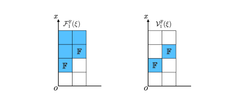
   Figure 1: Consider the one-dimensional multiset ${\xi=\{(1,1),(2,1)\}}$. This figure illustrates $\mathcal{F}_{1}^{\mathbb{F}}(\xi)$ and $\mathcal{V}_{1}^{\mathbb{F}}(\xi)$ over $\xi$ (see 3.7).

   

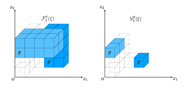
   Figure 2: Consider the two-dimensional multiset ${\xi=\{((0,2),1),((0,2),2),((2,0),1)\}}$. This figure illustrates $\mathcal{F}_{2}^{\mathbb{F}}(\xi)$ and $\mathcal{V}_{2}^{\mathbb{F}}(\xi)$ over $\xi$ (see 3.7).

3. Consider the two-dimensional multiset $\xi=\{((0,2),1),((0,2),2),((2,0),1)\}$. Then

   $$\mathcal{V}_{2}^{\mathbb{F}}(\xi)=\mathbb{F}(0,2)\oplus\mathbb{F}(0,2)\oplus\mathbb{F}(2,0)$$

   and

   $$\mathcal{F}_{2}^{\mathbb{F}}(\xi)=A_{2}^{\mathbb{F}}(0,2)\oplus A_{2}^{\mathbb{F}}(0,2)\oplus A_{2}^{\mathbb{F}}(2,0).$$

   This example is illustrated in Figure 2. Recall that $A_{2}^{\mathbb{F}}=\mathbb{F}[x_{1},x_{2}]$. The blue blocks represent the graded parts of $\mathcal{F}_{2}^{\mathbb{F}}(\xi)$ and $\mathcal{V}_{2}^{\mathbb{F}}(\xi)$. The blocks with an $\mathbb{F}$ are the locations of the homogeneous basis elements of $\mathcal{F}_{2}^{\mathbb{F}}(\xi)$ and $\mathcal{V}_{2}^{\mathbb{F}}(\xi)$. The third dimension parameterizes the number of direct summands. On the $x_{1},x_{2}$-axis we may read off the the degree of the blocks and we see how the generators are shifted. Moreover, the $x_{1},x_{2}$-axes on the left-hand side of the picture indicate that we can shift the degree or, in other words, that we can navigate through the module via multiplication by $x_{1},x_{2}$.

As one would expect, we have the following:

Definition, Proposition 3.8.

For any $V\in\mathbf{Grf}_{n}(\mathbb{F})$, there exists a finite $n$-dimensional multiset $\xi$ and a graded $\mathbb{F}$-vector space isomorphism

$$p:\mathcal{V}_{n}^{\mathbb{F}}(\xi)\xlongrightarrow{\sim}V.$$

The pair $(\mathcal{V}_{n}^{\mathbb{F}}(\xi),p)$ is unique in the following sense: if there exists another pair $(\mathcal{V}_{n}^{\mathbb{F}}(\xi^{\prime}),p^{\prime})$ such that $p^{\prime}:\mathcal{V}_{n}^{\mathbb{F}}(\xi^{\prime})\xlongrightarrow{\sim}V$ is a graded isomorphism, then

$$p^{-1}\circ p^{\prime}:\mathcal{V}_{n}^{\mathbb{F}}(\xi^{\prime})\xlongrightarrow{\sim}\mathcal{V}_{n}^{\mathbb{F}}(\xi)$$

is a graded isomorphism and we have $\xi=\xi^{\prime}$.

$$\Xi^{\mathbb{F}}_{n}(V):=\xi$$

is called the type of $V$.

Proof.

Let $G\subseteq V$ be a finite system of homogenous generators of the $n$-graded $\mathbb{F}$-vector space $V$ (such a set of homogeneous generators exists by 2.12) and choose a basis $B\subseteq G$. Then $B$ is a homogeneous basis of $V$. Now every $b\in B$ is of the form $b=b_{v}\in V_{v}$ for some unique $v\in{\mathbb{N}^{n}}$. This determines a finite $n$-dimensional mulitset $\xi$ and a graded isomorphism $p:\mathcal{V}_{n}^{\mathbb{F}}(\xi)\to V$. Formally, this is done as follows:

we can subdivide $B=\bigcup_{v\in T}\{b_{1,v},\dots,b_{d_{v},v}\}$ for a suitable subset $T\subseteq{\mathbb{N}^{n}}$ and suitable $d_{v}\in\mathbb{N}$ such that $b_{i,v}\in V_{v}$ for all $i\in\{1,\dots,d_{v}\}$ and all $v\in T$. Now define ${\xi:=\bigcup_{v\in T}\{(v,1),\dots,(v,d_{v})\}}$. So, $\xi=(T,\mu)$ where

$$\mu:T\longrightarrow\mathbb{N}_{\geq 1},\quad v\longmapsto d_{v}.$$

This leads to a graded isomorphism

$$p:\mathcal{V}_{n}^{\mathbb{F}}(\xi)\longrightarrow V,\quad e_{i,v}\longmapsto b_{i,v}$$

where $e_{i,v}$ is the $i$-th standard basis vector in $\mathbb{F}(v)^{\mu(v)}$.

If we have a second finite $n$-dimensional multiset $\xi^{\prime}$ together with a graded isomorphism $p^{\prime}:\mathcal{V}_{n}^{\mathbb{F}}(\xi^{\prime})\to V$, then $p\circ p^{\prime}:\mathcal{V}_{n}^{\mathbb{F}}(\xi^{\prime})\to\mathcal{V}_{n}^{\mathbb{F}}(\xi)$ is a graded isomorphism. So, we conclude that $\xi=\xi^{\prime}$. ∎

Remark 3.9.

Let $R$ be a commutative ring and $F$ be a finitely generated free $R$-module. Then any basis of $F$ has finite length and any two bases are of the same length. So, $\mathrm{rank}(F)$ (the rank of $F$) is well-defined and finite.

Definition, Proposition 3.10.

For any graded free $F\in\mathbf{Grf}_{n}(A_{n}^{\mathbb{F}})$, there exists an $n$-dimensional multiset $\xi$ and a graded $A_{n}^{\mathbb{F}}$-module isomorphism

$$p:\mathcal{F}_{n}^{\mathbb{F}}(\xi)\xlongrightarrow{\sim}F.$$

The pair $(\mathcal{F}_{n}^{\mathbb{F}}(\xi),p)$ is unique in the following sense: if there exists another pair $(\mathcal{F}_{n}^{\mathbb{F}}(\xi^{\prime}),p^{\prime})$ such that $p^{\prime}:\mathcal{F}_{n}^{\mathbb{F}}(\xi^{\prime})\xlongrightarrow{\sim}F$ is a graded isomorphism, then

$$p^{-1}\circ p^{\prime}:\mathcal{F}_{n}^{\mathbb{F}}(\xi^{\prime})\xlongrightarrow{\sim}\mathcal{F}_{n}^{\mathbb{F}}(\xi)$$

is a graded isomorphism and we have $\xi=\xi^{\prime}$.

$$\Xi^{\mathbb{F}}_{n}(F):=\xi$$

is called the type of $F$.

Proof.

Since $A_{n}^{\mathbb{F}}$ is commutative and $F$ is finitely generated graded free, $F$ admits a finite homogeneous $A_{n}^{\mathbb{F}}$-basis $B\subseteq F$. Now the argument is analogous as in the proof of 3.8: Every $b\in B$ is of the form $b=b_{v}\in F_{v}$ for some unique $v\in{\mathbb{N}^{n}}$. This determines a finite $n$-dimensional mulitset $\xi$ and a graded isomorphism $p:\mathcal{F}_{n}^{\mathbb{F}}(\xi)\to F$. Formally, this is done as follows:

we can subdivide $B=\bigcup_{v\in T}\{b_{1,v},\dots,b_{d_{v},v}\}$ for a suitable subset $T\subseteq{\mathbb{N}^{n}}$ and suitable $d_{v}\in\mathbb{N}$ such that $b_{i,v}\in F_{v}$ for all $i\in\{1,\dots,d_{v}\}$ and all $v\in T$. Now define ${\xi:=\bigcup_{v\in T}\{(v,1),\dots,(v,d_{v})\}}$. So, $\xi=(T,\mu)$ where

$$\mu:T\longrightarrow\mathbb{N}_{\geq 1},\quad v\longmapsto d_{v}.$$

This leads to an isomorphism of $n$-graded $A_{n}^{\mathbb{F}}$-modules

$$p:\mathcal{F}_{n}^{\mathbb{F}}(\xi)\longrightarrow F,\quad e_{i,v}\longmapsto b_{i,v}$$

where $e_{i,v}$ is the $i$-th standard basis vector in $A_{n}^{\mathbb{F}}(v)^{\mu(v)}$. If we have a second finite $n$-dimensional multiset $\xi^{\prime}$ together with a graded isomorphism $p^{\prime}:\mathcal{F}_{n}^{\mathbb{F}}(\xi^{\prime})\to F$, then $p\circ p^{\prime}:\mathcal{F}_{n}^{\mathbb{F}}(\xi^{\prime})\to\mathcal{F}_{n}^{\mathbb{F}}(\xi)$ is a graded isomorphism. So, we conclude that $\xi=\xi^{\prime}$. ∎

Figure 3: Illustration of the tensor-operation on $\mathcal{F}_{1}^{\mathbb{F}}(\xi)$ over the one-dimensional multiset $\xi=\{(1,1),(2,1)\}$ (continued from 3.7 and Figure 1).

3.2.2 The tensor-operation

There is a natural way to map objects in $\mathbf{Grf}_{n}(A_{n}^{\mathbb{F}})$ to objects in $\mathbf{Grf}_{n}(\mathbb{F})$ by means of the so-called tensor-operation. This tensor-operation will be necessary for the definition of free hulls (see 3.11). Let $M\in\mathbf{Grf}_{n}(A_{n}^{\mathbb{F}})$. Then

$$\mathbb{F}\otimes_{A_{n}^{\mathbb{F}}}M\in\mathbf{Grf}_{n}(\mathbb{F})$$

where for $u\in{\mathbb{N}^{n}}$, the $n$-grading is given by

$$\left(\mathbb{F}\otimes_{A_{n}^{\mathbb{F}}}M\right)_{u}:=\left\{\sum_{i=1}^{l}a_{i}\otimes m_{i}\,\bigg{|}\,a_{i}\in\mathbb{F},\,m_{i}\in M_{u}\right\}$$

(see also [MS04, p. 153]). Now

$$\mathbb{F}\otimes_{A_{n}^{\mathbb{F}}}-:\mathbf{Grf}_{n}(A_{n}^{\mathbb{F}})\longrightarrow\mathbf{Grf}_{n}(\mathbb{F})$$

is a right exact functor. We have a canonical isomorphism of finitely generated $n$-graded $\mathbb{F}$-vector spaces

$$\mathbb{F}\otimes_{A_{n}^{\mathbb{F}}}M\xlongrightarrow{\sim}M/\mathfrak{m}_{n}^{\mathbb{F}}M,\quad a\otimes m\longmapsto a\cdot\pi(m)$$ (1)

where $\pi:M\to M/\mathfrak{m}_{n}^{\mathbb{F}}M$ denotes the canonical projection. Note that $\pi$ is graded. We have

$$\mathcal{V}_{n}^{\mathbb{F}}(\xi)=\mathcal{F}_{n}^{\mathbb{F}}(\xi)/\mathfrak{m}_{n}^{\mathbb{F}}\mathcal{F}_{n}^{\mathbb{F}}(\xi)$$

for any finite $n$-dimensional multiset $\xi$. So, (1) yields an isomorphism of $n$-graded $\mathbb{F}$-vector spaces

$$\mathbb{F}\otimes_{A_{n}^{\mathbb{F}}}\mathcal{F}_{n}^{\mathbb{F}}(\xi)\xlongrightarrow{\sim}\mathcal{V}_{n}^{\mathbb{F}}(\xi).$$

The tensor-operation is illustrated in Figures 3 and 4.

Figure 4: Illustration of the tensor-operation on $\mathcal{F}_{2}^{\mathbb{F}}(\xi)$ over the two-dimensional multiset $\xi=\{((0,2),1),((0,2),2),((2,0),1)\}$ (continued from 3.7 and Figure 2).

3.2.3 The main theorem on free hulls

Using the tensor operation, we can now define free hulls:

Definition 3.11 ([CZ09, Def. 4], [CZ07, Sec. 4.2], Free hull).

A free hull of ${M\in\mathbf{Grf}_{n}(A_{n}^{\mathbb{F}})}$ is a pair $(F,p)$, where $p$ is a surjective graded $A_{n}^{\mathbb{F}}$-module homomorphism $p:F\to M$ and $F\in\mathbf{Grf}_{n}(A_{n}^{\mathbb{F}})$ is graded free such that

$$\mathrm{id}_{\mathbb{F}}\otimes_{A_{n}^{\mathbb{F}}}p:\mathbb{F}\otimes_{A_{n}^{\mathbb{F}}}F\xlongrightarrow{\sim}\mathbb{F}\otimes_{A_{n}^{\mathbb{F}}}M$$

is an isomorphism of $n$-graded $\mathbb{F}$-vector spaces.

The main goal for the rest of Section 3.2 is to prove the following theorem, the main theorem on free hulls, which states that free hulls exsist and that they are unique up to isomorphism.

Theorem 3.12 ([CZ09, Thm. 7], [CZ07, Sec. 4.2]).

Every $M\in\mathbf{Grf}_{n}(A_{n}^{\mathbb{F}})$ admits a free hull

$$p:\mathcal{F}^{\mathbb{F}}_{n}(\xi)\longrightarrow M$$

for a finite $n$-dimensional multiset $\xi$. If $M$ is graded free, then $p$ is a graded isomorphism. Free hulls are unique in the following sense: if $p:F\to M$ and $p^{\prime}:F^{\prime}\to M$ are free hulls of $M$, then there exists a graded isomorphism $\psi:F\xlongrightarrow{\sim}F^{\prime}$ such that the diagram

commutes. In particular, if $F=\mathcal{F}^{\mathbb{F}}_{n}(\xi)$ and $F^{\prime}=\mathcal{F}^{\mathbb{F}}_{n}(\xi^{\prime})$ for two finite $n$-dimensional multisets $\xi$ and $\xi^{\prime}$, then $\xi=\xi^{\prime}$.

In comparison to [CZ09, Thm. 7] and [CZ07, Sec. 4.2], we just have added a few technical details to the formulation of 3.12. In [CZ09, Thm. 7] and [CZ07, Sec. 4.2], the authors give a sketch of the proof of 3.12. The proof of 3.12 requires some preparations and will be elaborated throughout Sections 3.2.4-3.2.6. The key to the proof is an $n$-graded version of Nakayama’s lemma.

Note that in 3.12, the map $\psi$ is generally not unique. This is demonstrated by the next example.

Example 3.13.

Recall that $A_{1}^{\mathbb{F}}=\mathbb{F}[x]$. Consider $F:=\mathbb{F}[x](1)\oplus\mathbb{F}[x](2)$. Then $F$ is graded free and $B:=\{(1,0),(x,1)\}$ and $B^{\prime}:=\{(1,0),(0,1)\}$ are homogeneous $\mathbb{F}[x]$-bases of $F$. Now

$$f:F\xlongrightarrow{\sim}F, \quad(1,0)\longmapsto(1,0)$$

$$\quad(0,1)\longmapsto(0,1)$$

$$f^{\prime}:F\xlongrightarrow{\sim}F, \quad(1,0)\longmapsto(1,0)$$

$$\quad(0,1)\longmapsto(x,1)$$

are graded isomorphisms with $f\neq f^{\prime}$ and $\mathrm{id}_{\mathbb{F}}\otimes_{\mathbb{F}[x]}f=\mathrm{id}_{\mathbb{F}}\otimes_{\mathbb{F}[x]}f^{\prime}$. This is due to the fact that for all $a\in\mathbb{F}$,

$$a\otimes(x,1) =a\otimes(x,0)+a\otimes(0,1)=a\otimes x\cdot(1,0)+a\otimes(0,1)$$

$$=a\cdot x\otimes(1,0)+a\otimes(0,1)=0\otimes(1,0)+a\otimes(0,1)=a\otimes(0,1),$$

where $a\cdot x=x\cdot a=0$ for all $a\in\mathbb{F}$ by definition of the $\mathbb{F}[x]$-module structure on $\mathbb{F}$.

Before we proceed with the elaboration of the proof of 3.12, we give an example which illustrates the concept of free hulls in two dimensions.

Example 3.14.

This example is illustrated in Figure 5. Recall that $A_{2}^{\mathbb{F}}=\mathbb{F}[x_{1},x_{2}]$. Consider the graded submodule

$$M :=\braket{x_{1}^{3},x_{1}^{2}x_{2},x_{1}x_{2}^{2},x_{2}^{3}}_{A^{\mathbb{F}}_{2}}\subseteq A^{\mathbb{F}}_{2}.$$

Now

$$G:=\{x_{1}^{3},x_{1}^{2}x_{2},x_{1}x_{2}^{2},x_{2}^{3}\}\subseteq M$$

is a minimal set of homogeneous generators of $M$. We have

$$\mathrm{deg}(x_{1}^{3})=(3,0),\quad\mathrm{deg}(x_{1}^{2}x_{2})=(2,1),\quad\mathrm{deg}(x_{1}x_{2}^{2})=(1,2),\quad\mathrm{deg}(x_{2}^{3})=(0,3).$$

$M$ is not graded free (in 3.20, we will see that for ${M\in\mathbf{Grf}_{n}(A_{n}^{\mathbb{F}})}$ graded free is equivalent to free). If $M$ were graded free, then any minimal set of homogeneous generators would be a basis (see 3.18). But consider for example

$$x_{1}\cdot x_{1}x_{2}^{2}=x_{1}^{2}x_{2}^{2}=x_{2}\cdot x_{1}^{2}x_{2}.$$

As we can see, $x_{1}^{2}x_{2}^{2}$ is not a unique $A_{2}^{\mathbb{F}}$-linear combination of elements in $G$. Hence, $G$ is not a basis of $M$ and since $G$ is minimal, $M$ is therefore not graded free. The fact that $x_{1}^{2}x_{2}^{2}$ can be obtained by shifting different generators is illustrated in Figure 5 by different shades of the colour blue. These different shades indicate that we may have an overlap if we shift different generators.

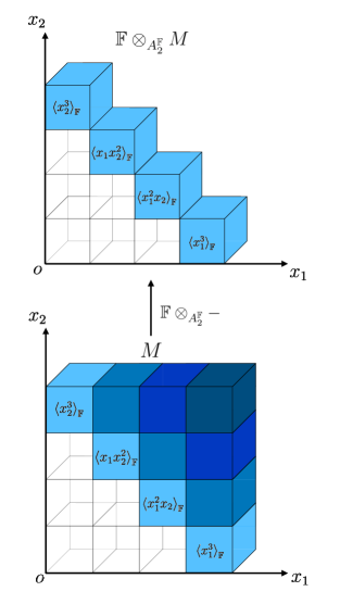
Figure 5: Illustration of 3.14.

Now consider the two-dimensional multiset

$$\xi=(V,\mu)=\{((3,0),1),((2,1),1),((1,2),1),((0,3),1)\}$$

where $V=\{(3,0),(2,1),(1,2),(0,3)\}\subseteq\mathbb{N}^{2}$ and where the mulitplicity function $\mu$ is given by ${\mu(3,0)=\mu(2,1)=\mu(1,2)=\mu(0,3)=1}$. We have

$$\mathcal{F}_{2}^{\mathbb{F}}(\xi)=A_{2}^{\mathbb{F}}(3,0)\oplus A_{2}^{\mathbb{F}}(2,1)\oplus A_{2}^{\mathbb{F}}(1,2)\oplus A_{2}^{\mathbb{F}}(0,3)$$

and

$$p:\mathcal{F}_{2}^{\mathbb{F}}(\xi) \longrightarrow M,$$

$$(1,0,0,0) \longmapsto x_{1}^{3},$$

$$(0,1,0,0) \longmapsto x_{1}^{2}x_{2},$$

$$(0,0,1,0) \longmapsto x_{1}x_{2}^{2},$$

$$(0,0,0,1) \longmapsto x_{2}^{3}$$

defines a surjective graded $A_{2}^{\mathbb{F}}$-module homomorphism. We claim that $(\mathcal{F}_{2}^{\mathbb{F}}(\xi),p)$ is a free hull of $M$:

since $p$ is surjective and tensoring is right exact,

$$\mathrm{id}_{\mathbb{F}}\otimes_{A_{2}^{\mathbb{F}}}p:\mathbb{F}\otimes_{A_{2}^{\mathbb{F}}}\mathcal{F}_{2}^{\mathbb{F}}(\xi)\longrightarrow\mathbb{F}\otimes_{A_{2}^{\mathbb{F}}}M$$

is a surjective graded $\mathbb{F}$-vector space homomorphism. If we want to show that $(\mathcal{F}_{2}^{\mathbb{F}}(\xi),p)$ is a free hull of $M$ we have to show that $\mathrm{id}_{\mathbb{F}}\otimes_{A_{2}^{\mathbb{F}}}p$ is an isomorphism. Since $\mathrm{id}_{\mathbb{F}}\otimes_{A_{2}^{\mathbb{F}}}p$ is graded and surjective, $\mathrm{id}_{\mathbb{F}}\otimes_{A_{2}^{\mathbb{F}}}p$ induces surjective $\mathbb{F}$-vector space homomorphisms

$$(\mathrm{id}_{\mathbb{F}}\otimes_{A_{2}^{\mathbb{F}}}p)_{v}:\left(\mathbb{F}\otimes_{A_{2}^{\mathbb{F}}}\mathcal{F}_{2}^{\mathbb{F}}(\xi)\right)_{v}\longrightarrow\left(\mathbb{F}\otimes_{A_{2}^{\mathbb{F}}}M\right)_{v}$$

for all $v\in\mathbb{N}^{2}$. So, it suffices to show that $(\mathrm{id}_{\mathbb{F}}\otimes_{A_{2}^{\mathbb{F}}}p)_{v}$ is an isomorphism for all $v\in\mathbb{N}^{2}$. For this, it suffices to show that

$$\mathrm{dim}_{\mathbb{F}}\left(\left(\mathbb{F}\otimes_{A_{2}^{\mathbb{F}}}\mathcal{F}_{2}^{\mathbb{F}}(\xi)\right)_{v}\right)=\mathrm{dim}_{\mathbb{F}}\left(\left(\mathbb{F}\otimes_{A_{2}^{\mathbb{F}}}M\right)_{v}\right)$$

for all $v\in\mathbb{N}^{2}$.

Since $\mathbb{F}\otimes_{A_{2}^{\mathbb{F}}}\mathcal{F}_{2}^{\mathbb{F}}(\xi)\cong\mathcal{V}_{2}^{\mathbb{F}}(\xi)$ as bigraded $\mathbb{F}$-vector spaces and since $(\mathrm{id}_{\mathbb{F}}\otimes_{A_{2}^{\mathbb{F}}}p)_{v}$ is surjective, we obtain

$$0\leq\mathrm{dim}_{\mathbb{F}}\left(\left(\mathbb{F}\otimes_{A_{2}^{\mathbb{F}}}M\right)_{v}\right)\leq\mathrm{dim}_{\mathbb{F}}\left(\left(\mathbb{F}\otimes_{A_{2}^{\mathbb{F}}}\mathcal{F}_{2}^{\mathbb{F}}(\xi)\right)_{v}\right)=\mathrm{dim}_{\mathbb{F}}\left(\mathcal{V}_{2}^{\mathbb{F}}(\xi)_{v}\right)$$ (2)

for all $v\in\mathbb{N}^{2}$. Since $\mathrm{dim}_{\mathbb{F}}\left(\mathcal{V}_{2}^{\mathbb{F}}(\xi)_{v}\right)=0$ for all $v\in\mathbb{N}^{2}\setminus V$, (2) shows that

$$\mathrm{dim}_{\mathbb{F}}\left(\left(\mathbb{F}\otimes_{A_{2}^{\mathbb{F}}}M\right)_{v}\right)=\mathrm{dim}_{\mathbb{F}}\left(\left(\mathbb{F}\otimes_{A_{2}^{\mathbb{F}}}\mathcal{F}_{2}^{\mathbb{F}}(\xi)\right)_{v}\right)=\mathrm{dim}_{\mathbb{F}}\left(\mathcal{V}_{2}^{\mathbb{F}}(\xi)_{v}\right)=0$$

for all $v\in\mathbb{N}^{2}\setminus V$.

Let $v\in V$. We have

$$\mathrm{dim}_{\mathbb{F}}\left(\left(\mathbb{F}\otimes_{A_{2}^{\mathbb{F}}}\mathcal{F}_{2}^{\mathbb{F}}(\xi)\right)_{v}\right)=\mathrm{dim}_{\mathbb{F}}\left(\mathcal{V}_{2}^{\mathbb{F}}(\xi)_{v}\right)=1.$$

So, we have to show that

$$\mathrm{dim}_{\mathbb{F}}\left(\left(\mathbb{F}\otimes_{A_{2}^{\mathbb{F}}}M\right)_{v}\right)=1.$$

(2) implies that

$$0\leq\mathrm{dim}_{\mathbb{F}}\left(\left(\mathbb{F}\otimes_{A_{2}^{\mathbb{F}}}M\right)_{v}\right)\leq 1.$$

So, it suffices to show that $\left(\mathbb{F}\otimes_{A_{2}^{\mathbb{F}}}M\right)_{v}\neq 0$. We have $M_{v}=\braket{x^{v}}_{\mathbb{F}}$. Consider

$$1\otimes x^{v}\in\left(\mathbb{F}\otimes_{A_{2}^{\mathbb{F}}}M\right)_{v}.$$

Then $1\otimes x^{v}\neq 0$. This is due to the fact that under the canonical graded isomorphism

$$\mathbb{F}\otimes_{A_{2}^{\mathbb{F}}}M\xlongrightarrow{\sim}M/\mathfrak{m}_{2}^{\mathbb{F}}M,\quad a\otimes m\longmapsto a\cdot\pi(m)$$

the image of $1\otimes x^{v}$ in $M/\mathfrak{m}_{2}^{\mathbb{F}}M$ is not zero.

As 3.14 indicates, a free hull of $M\in\mathbf{Grf}_{n}(A_{n}^{\mathbb{F}})$ is given as follows: choose a minimal set of homogeneous generators $G\subseteq M$. This determines a finite $n$-dimensional multiset $\xi$ and a surjective graded morphism $p:\mathcal{F}_{n}^{\mathbb{F}}(\xi)\to M$. The multiset $\xi$ tells us in which degrees the generators in $G$ are located. Throughout Sections 3.2.4-3.2.6, we will see that this approach is the right one. We close this section with the next definition. Since free hulls are unique up to isomorphism by 3.12, the next definition makes sense.

Definition 3.15 (Type).

Let $M\in\mathbf{Grf}_{n}(A_{n}^{\mathbb{F}})$ and let $p:\mathcal{F}_{n}^{\mathbb{F}}(\xi)\to M$ be a free hull of $M$. Then

$$\Xi_{n}^{\mathbb{F}}(M):=\xi$$

is called the type of $M$. Note that

$$\Xi_{n}^{\mathbb{F}}(M)=\Xi_{n}^{\mathbb{F}}(\mathbb{F}\otimes_{A_{n}^{\mathbb{F}}}M).$$

3.2.4 The n-graded Nakayama Lemma

The following $n$-graded version of Nakayama’s Lemma can be found in [MS04, Ex. 7.8]. Note that in [MS04, Ex. 7.8], the setting is more general.

Lemma 3.16 ([MS04, Ex. 7.8], Nakayama).

Let $M\in\mathbf{Grf}_{n}(A_{n}^{\mathbb{F}})$, $m_{1},\dots,m_{d}\in M$ be homogeneous elements and denote by $\pi:M\to M/\mathfrak{m}_{n}^{\mathbb{F}}M$ the canonical projection. Note that $\pi$ is graded.

1. $m_{1},\dots,m_{d}$ generate $M$ if and only if $\pi(m_{1}),\dots,\pi(m_{d})$ generate the finitely generated $n$-graded $\mathbb{F}$-vector space $M/\mathfrak{m}_{n}^{\mathbb{F}}M$.

2. $\{m_{1},\dots,m_{d}\}$ is a minimal generating set of $M$ if and only if $\{\pi(m_{1}),\dots,\pi(m_{d})\}$ is an $\mathbb{F}$-basis of $M/\mathfrak{m}_{n}^{\mathbb{F}}M$.

3. Let $G\subseteq M$ be a minimal set of homogeneous generators (such a $G$ always exists and is finite by 2.12). If $C\subseteq M$ is another minimal set of homogeneous generators, then $\left\lvert C\right\lvert=\left\lvert G\right\lvert$.

Proof.

The idea of the proof is similar to the $\mathbb{N}$-graded setting (see [Eis05, Lem. 1.4]). We clearly have that if $m_{1},\dots,m_{d}$ generate $M$, then $\pi(m_{1}),\dots,\pi(m_{d})$ generate $M/\mathfrak{m}_{n}^{\mathbb{F}}M$.

So let us prove the converse: Assume that $\pi(m_{1}),\dots,\pi(m_{d})$ generate $M/\mathfrak{m}_{n}^{\mathbb{F}}M$. Let ${\overline{M}:=M/\braket{m_{1},\dots,m_{d}}_{A_{n}^{\mathbb{F}}}}$. Since ${\braket{m_{1},\dots,m_{d}}_{A_{n}^{\mathbb{F}}}\subseteq M}$ is graded, $\overline{M}$ is finitely generated and $n$-graded (as it is generated by finitely many homogeneous elements (see 2.13)). Since $\pi(m_{1}),\dots,\pi(m_{d})$ generate $M/\mathfrak{m}_{n}^{\mathbb{F}}M$, $\overline{M}/\mathfrak{m}_{n}^{\mathbb{F}}\overline{M}=0$. Hence, $\overline{M}=\mathfrak{m}_{n}^{\mathbb{F}}\overline{M}$. Now $\overline{M}$ has a non-empty finite set of homogeneous generators

$$\bigcup_{v\in V}\{z_{1,v},\dots,z_{d_{v},v}\}\subseteq\overline{M}$$

for a suitable finite $V\subseteq\mathbb{N}^{n}$ with $z_{i,v}\in\overline{M}_{v}$ for all $v\in V$ and all $i\in\{1,\dots,d_{v}\}$. The goal is to show that $z_{i,u}=0$ for all $u\in V$ and all $i\in\{1,\dots,d_{u}\}$.

Let $Z_{1}\subseteq V$ be the set of all $v\in V$ that are minimal with respect to the partial order $\preceq$. Then $\left(\mathfrak{m}_{n}^{\mathbb{F}}\overline{M}\right)_{w}=\overline{M}_{w}=0$ for all $w\in{\mathbb{N}^{n}}\setminus\bigcup_{v\in V}\mathbb{N}^{n}_{\succeq v}$. Let $u\in Z_{1}$ and $j\in\{1,\dots,d_{u}\}$. Since $\overline{M}=\mathfrak{m}_{n}^{\mathbb{F}}\overline{M}$, we can write

$$z_{j,u}=\sum_{v\in V}\sum_{i=1}^{d_{v}}s^{(i,v)}r^{(i,v)}z_{i,v}$$

where $s^{(i,v)}\in A_{n}^{\mathbb{F}}$ and $r^{(i,v)}\in\mathfrak{m}_{n}^{\mathbb{F}}$. Since $\mathfrak{m}_{n}^{\mathbb{F}}=\bigoplus_{v\in{\mathbb{N}^{n}_{\succ 0}}}(A_{n}^{\mathbb{F}})_{v}$, we have

$$s^{(i,v)}r^{(i,v)}z_{i,v}=\left(\sum_{w\in\mathbb{N}^{n}}s^{(i,v)}_{w}\right)\left(\sum_{w\in{\mathbb{N}}_{\succ 0}^{n}}r^{(i,v)}_{w}\right)z_{i,v}=\sum_{u\in{\mathbb{N}^{n}}}\sum_{w\succ 0,y+w=u}s^{(i,v)}_{y}r^{(i,v)}_{w}z_{i,v}$$

for unique $s^{(i,v)}_{w},r^{(i,v)}_{w}\in(A_{n}^{\mathbb{F}})_{w}$ with $s^{(i,v)}_{w}=0$ for all but finitely many $w\in\mathbb{N}^{n}$ and $r^{(i,v)}_{w}=0$ for all but finitely many $w\in{\mathbb{N}^{n}_{\succ 0}}$. If $s^{(i,v)}r^{(i,v)}z_{i,v}\neq 0$, then all nonzero homogeneous parts of $s^{(i,v)}r^{(i,v)}z_{i,v}$ have degree $\succ u$. Since $u$ is minimal, this implies that $z_{j,u}=0$. Therefore,

$$\bigcup_{v\in V}\{z_{1,v},\dots,z_{d_{v},v}\}\setminus\bigcup_{v\in Z_{1}}\{z_{1,v},\dots,z_{d_{v},v}\}\subseteq\overline{M}$$

is a set of homogeneous generators of $\overline{M}$. Now repeat the same procedure for

$$\bigcup_{v\in V}\{z_{1,v},\dots,z_{d_{v},v}\}\setminus\bigcup_{v\in Z_{1}}\{z_{1,v},\dots,z_{d_{v},v}\}\subseteq\overline{M}$$

Then $z_{i,v}=0$ for all $v\in Z_{1}\cup Z_{2}$ and all $i\in\{1,\dots,d_{v}\}$, where $Z_{2}$ denotes the set of all $v\in V\setminus Z_{1}$ that are minimal with respect to $\preceq$. Now proceed inductively. Since $V$ is finite, there exists an $m\in\mathbb{N}$ such that $V=\bigcup_{i=1}^{m}Z_{i}$ and we conclude that $z_{i,v}=0$ for all $v\in V$ and all $i\in\{1,\dots,d_{v}\}$. So $\overline{M}=0$, which proves that $m_{1},\dots,m_{d}$ generate $M$.

For the second part, let us first assume that $\{m_{1},\dots,m_{d}\}\subseteq M$ is minimal and that ${\{\pi(m_{1}),\dots,\pi(m_{d})\}\subseteq M/\mathfrak{m}_{n}^{\mathbb{F}}M}$ is not minimal. Then there exists an $i\in\{1,\dots,d\}$ such that $\{\pi(m_{1}),\dots,\pi(m_{d})\}\setminus\{\pi(m_{i})\}$ is a generating set of $M/\mathfrak{m}_{n}^{\mathbb{F}}M$. By using the first part of this lemma, this implies that $\{m_{1},\dots,m_{d}\}\setminus\{m_{i}\}$ is a generating set of $M$. But this is a contradiction to the minimality of $m_{1},\dots,m_{d}$. Thus, $\{\pi(m_{1}),\dots,\pi(m_{d})\}$ is a minimal generating set and hence an $\mathbb{F}$-basis of $M/\mathfrak{m}_{n}^{\mathbb{F}}M$.

$\{\pi(m_{1}),\dots,\pi(m_{d})\}$ is an $\mathbb{F}$-basis of $M/\mathfrak{m}_{n}^{\mathbb{F}}$ if and only if $\{\pi(m_{1}),\dots,\pi(m_{d})\}$ is a minimal generating set. As before, if $\{m_{1},\dots,m_{d}\}$ were not minimal this would be a contradiction to the minimality of $\{\pi(m_{1}),\dots,\pi(m_{d})\}$.

The third part is clear by the second part since all minimal generating sets (or equivalently $\mathbb{F}$-bases) of $M/\mathfrak{m}_{n}^{\mathbb{F}}$ are finite and of the same length. ∎

3.2.5 Existence of free hulls

The next Lemma is a standard result about Noetherian modules.

Lemma 3.17.

Let $R$ be a commutative Noetherian ring and let $N$ be a Noetherian $R$-module. Let $f:N\to N$ be a surjective $R$-module endomorphism. Then $f$ is an automorphism.

Proof.

We have to show that $f$ is injective. We have $\mathrm{ker}(f^{r})\subseteq\mathrm{ker}(f^{r+1})$ for all $r\in\mathrm{N}$. Since $N$ is Noetherian there exists an $m\in\mathbb{N}$ such that $\mathrm{ker}(f^{m})=\mathrm{ker}(f^{m+r})$ for all $r\geq m$. As $f$ is surjective, we have $\mathrm{im}(f^{n})=N$. Now we show that $\mathrm{im}(f^{m})\cap\mathrm{ker}(f^{m})=0$. Let $x\in\mathrm{im}(f^{m})\cap\mathrm{ker}(f^{m})$. Then $f^{m}(x)=0$ and $f^{m}(y)=x$ for some $y\in N$ since $f$ is surjective. Hence, $f^{2m}(y)=0$. Since $\mathrm{ker}(f^{m})=\mathrm{ker}(f^{2m})$, we have $x=f^{m}(y)=0$. ∎

Proposition 3.18.

Let $F\in\mathbf{Grf}_{n}(A_{n}^{\mathbb{F}})$ be free as an $A_{n}^{\mathbb{F}}$-module and let $G\subseteq F$ be a minimal set of homogeneous generators of $F$ (such a $G$ always exists and is finite by 2.12). Then $G$ is a homogeneous basis of $F$.

Proof.

$A_{n}^{\mathbb{F}}$ is commutative and $F$ is free and finitely generated. So, $\mathrm{rank}(F)$ is finite and well-defined (see 3.9). Suppose that $\mathrm{rank}(F)=d$ and let $B=\{b_{1},\dots,b_{d}\}$ be an $A_{n}^{\mathbb{F}}$-basis of $F$. We have $\mathrm{dim}_{\mathbb{F}}(\mathbb{F}\otimes_{A_{n}^{\mathbb{F}}}F)=d$ and

$$\mathbb{F}\otimes_{A_{n}^{\mathbb{F}}}F=A_{n}^{\mathbb{F}}/\mathfrak{m}^{\mathbb{F}}_{n}\otimes_{A_{n}^{\mathbb{F}}}F\cong F/\mathfrak{m}^{\mathbb{F}}_{n}F$$

which shows that $\mathrm{dim}_{\mathbb{F}}(F/\mathfrak{m}^{\mathbb{F}}_{n}F)=d$. Thus, $\left\lvert G\right\lvert=d$ by 3.16. So, there exists a set-theoretic bijection $\tau:B\to G$. Now $\tau$ induces a surjective $A_{n}^{\mathbb{F}}$-module endomorphism

$$f_{\tau}:F\longrightarrow F,\quad\sum_{i=1}^{d}a_{i}b_{i}\longmapsto\sum_{i=1}^{d}a_{i}\tau(b_{i}).$$

Since $A_{n}^{\mathbb{F}}$ is Noetherian and $F$ is finitely generated, $F$ is a Noetherian $A_{n}^{\mathbb{F}}$-module. Thus, $f_{\tau}$ has to be an automorphism by 3.17. Hence, $G$ is an $A_{n}^{\mathbb{F}}$-basis of $F$. $G$ consists only of homogeneous elements by assumption. So, $G$ is a homogeneous $A_{n}^{\mathbb{F}}$-basis of $F$. ∎

Proposition 3.19.

For $M\in\mathbf{Grf}_{n}(A_{n}^{\mathbb{F}})$, the following statements are equivalent:

1. $M$ is graded free as an $A_{n}^{\mathbb{F}}$-module.

2. $M$ is free as an $A_{n}^{\mathbb{F}}$-module.

Proof.

$(1.\Longrightarrow 2.)$ is clear and $(2.\Longrightarrow 1.)$ follows from 3.18. ∎

Proposition 3.20.

Let $F,M\in\mathbf{Grf}_{n}(A_{n}^{\mathbb{F}})$ with $F$ graded free. Let $p:F\to M$ be a surjective graded morphism. The following statements are equivalent:

1. $p:F\to M$ is a free hull of $M$.

2. for any homogeneous basis $B$ of $F$, $p(B)$ is a minimal set of homogeneous generators of $M$ with $\left\lvert p(B)\right\lvert=\left\lvert B\right\lvert$.

3. there exists a homogeneous basis $B$ of $F$ such that $p(B)$ is a minimal set of homogeneous generators of $M$ with $\left\lvert p(B)\right\lvert=\left\lvert B\right\lvert$.

Proof.

Since $\mathbb{F}\otimes_{A_{n}^{\mathbb{F}}}-$ is right exact, we obtain a surjective graded morphism

$$\mathrm{id}_{\mathbb{F}}\otimes_{A_{n}^{\mathbb{F}}}p:\mathbb{F}\otimes_{A_{n}^{\mathbb{F}}}F\longrightarrow\mathbb{F}\otimes_{A_{n}^{\mathbb{F}}}M.$$

Now we obtain a commutative diagram in $\mathbf{Grf}_{n}(\mathbb{F})$

(3)

where the vertical maps are all graded isomorphisms and the horizontal maps are all graded surjective morphisms. If we identify $\mathbb{F}\otimes_{A_{n}^{\mathbb{F}}}F=F/F\mathfrak{m}_{n}^{\mathbb{F}}$ and ${\mathbb{F}\otimes_{A_{n}^{\mathbb{F}}}M=M/M\mathfrak{m}_{n}^{\mathbb{F}}}$ along the vertical graded ismorphisms in (3), we obtain a commutative diagram

where $\pi_{F}:F\to F/\mathfrak{m}_{n}^{\mathbb{F}}F=\mathbb{F}\otimes_{A_{n}^{\mathbb{F}}}F$ and $\pi_{M}:M\to M/\mathfrak{m}_{n}^{\mathbb{F}}M=\mathbb{F}\otimes_{A_{n}^{\mathbb{F}}}M$ denotes the canonical projections.

$(1.\Longrightarrow 2.)$: Since $p:F\to M$ is a free hull, we know that $\mathrm{id}\otimes_{A_{n}^{\mathbb{F}}}p$ has to be a graded isomorphism. Using the commutativity of (3), this implies that $F/\mathfrak{m}_{n}^{\mathbb{F}}\to M/\mathfrak{m}_{n}^{\mathbb{F}}M$ is a graded isomorphism. Now let $B$ be a homogeneous $A_{n}^{\mathbb{F}}$-basis of $F$. Then $B$ is finite and $\pi_{F}(B)$ is a homogenenous $\mathbb{F}$-basis of $\mathbb{F}\otimes_{A_{n}^{\mathbb{F}}}F$ by 3.16 and $\left\lvert\pi_{F}(B)\right\lvert=\left\lvert B\right\lvert$. Hence, $C:=(\mathrm{id}_{\mathbb{F}}\otimes_{A_{n}^{\mathbb{F}}}p)(\pi_{F}(B))$ is a homogeneous $\mathbb{F}$-basis of $\mathbb{F}\otimes_{A_{n}^{\mathbb{F}}}M$. Since $p$ is surjective and graded, $p(B)\subseteq M$ is a set of homogeneous generators of $M$. Since $\pi_{M}(p(B))=C$, we conclude that

$$\left\lvert B\right\lvert\geq\left\lvert p(B)\right\lvert\geq\left\lvert\pi_{M}(p(B))\right\lvert\geq\left\lvert C\right\lvert=\left\lvert(\mathrm{id}_{\mathbb{F}}\otimes_{A_{n}^{\mathbb{F}}}p)(\pi_{F}(B))\right\lvert=\left\lvert\pi_{F}(B)\right\lvert=\left\lvert B\right\lvert.$$

Hence, $\left\lvert p(B)\right\lvert=\left\lvert\pi_{M}(p(B))\right\lvert=\left\lvert C\right\lvert=\left\lvert B\right\lvert$. By using 3.16, this implies that $p(B)$ is minimal.

$(2.\Longrightarrow 1.)$: Let $B\subseteq F$ be a homogeneous basis of $F$ such that $p(B)$ is a minimal generating system of $M$ with $\left\lvert p(B)\right\lvert=\left\lvert B\right\lvert$ ($B$ and $p(B)$ are finite). By 3.16, $\pi_{M}(p(B))$ is an $\mathbb{F}$-basis of $M/\mathfrak{m}^{\mathbb{F}}_{n}M$ with $\left\lvert\pi_{M}(p(B))\right\lvert=\left\lvert p(B)\right\lvert$ and $\pi_{F}(B)$ is an $\mathbb{F}$-basis of $F/\mathfrak{m}^{\mathbb{F}}_{n}F$ with $\left\lvert\pi_{F}(B)\right\lvert=\left\lvert B\right\lvert$. Therefore,

$$\left\lvert\pi_{F}(B)\right\lvert=\left\lvert B\right\lvert=\left\lvert p(B)\right\lvert=\left\lvert\pi_{M}(p(B))\right\lvert$$

which shows that the horizontal maps in (3) are graded isomorphisms.

$F$ has a homogenous basis $B$ since $F$ is graded free which shows that $(2.\Longrightarrow 3.)$. $(3.\Longrightarrow 1.)$: Assume that $F$ has a homogenous basis $B\subseteq F$ such that $p(B)$ is a minimal set of homogeneous generators of $M$ with $\left\lvert B\right\lvert=\left\lvert p(B)\right\lvert$. Now the proof is analogous to $(2.\Longrightarrow 1.)$. ∎

We are now ready to prove the existence of free hulls:

Proof of 3.12, existence.

Let $G=\{m_{1},\dots,m_{d}\}$ be a minimal set of homogenous generators of $M$. Then we can subdivide $G=\bigcup_{v\in T}\{m_{1,v},\dots,m_{d_{v},v}\}$ for a suitable subset $T\subseteq{\mathbb{N}^{n}}$ and suitable $d_{v}\in\mathbb{N}$ such that $m_{i,v}\in M_{v}$ for all $i\in\{1,\dots,d_{v}\}$ and all $v\in T$. Now define $\xi:=\bigcup_{v\in T}\{(v,1),\dots,(v,d_{v})\}$. So, $\xi=(T,\mu)$ defines an $n$-dimensional multiset where

$$\mu:T\longrightarrow\mathbb{N}_{\geq 1},\quad v\longmapsto d_{v}.$$

This leads to a surjective graded morphism

$$p:\mathcal{F}_{n}^{\mathbb{F}}(\xi)\longrightarrow M,\quad e_{i,v}\longmapsto m_{i,v}$$

where $e_{i,v}$ is the $i$-th standard basis vector in $A_{n}^{\mathbb{F}}(v)^{\mu(v)}$. Now $p:\mathcal{F}_{n}^{\mathbb{F}}(\xi)\to M$ is a free hull by 3.20. In particular, if $M$ is graded free, then $p$ is a graded isomorphism (see proof of 3.10). ∎

3.2.6 Uniqueness of free hulls

Before we proof the uniqueness of free hulls, we need the following:

Proposition 3.21.

Let $R$ be an $n$-graded commutative ring and let $M,N,P$ be $n$-graded $R$-modules.

1. Let $g:M\to N$ and $f:P\to N$ be graded $R$-module homomorphisms. If $h:P\to M$ is an $R$-module homomorphism such that $f=g\circ h$, then there exists a graded $R$-module homomorphism $\psi:P\to M$ such that $f=g\circ\psi$.

2. If $P$ is projecive, then $P$ is graded projective, i.e. if $g:M\to N$ is a surjective graded $R$-module homomorphism and if $f:P\to N$ is a graded $R$-module homomorphism, then there exists a graded $R$-module homomorphism ${\psi:P\to M}$ such that $f=g\circ\psi$.

3. If $P$ is graded free, then $P$ is graded projective.

Proof.

Let us start with the proof of the first part: for this, let $y\in P$. Then $\psi(y)\in M$ is constructed as follows: we have $y=\sum_{v\in{\mathbb{N}^{n}}}y_{v}$ for unique $y_{v}\in P_{v}$ with $y_{v}=0$ for all but finitely many $v\in{\mathbb{N}^{n}}$. Let $v\in{\mathbb{N}^{n}}$. Since $f$ is graded, we have $f(y_{v})\in N_{v}$. It holds that $h(y_{v})=\sum_{w\in{\mathbb{N}^{n}}}z_{w}$ for unique $z_{w}\in M_{w}$ with $z_{w}=0$ for all but finitely many $w\in{\mathbb{N}^{n}}$. Now we have

$$f(y_{v})=g(h(y_{v}))=\sum_{w\in{\mathbb{N}^{n}}}g(z_{w})\in N_{v}$$

which implies that (since $g$ is graded) $g(z_{w})=0$ for all $v\neq w$. So, we have $f(y_{v})=g(z_{v})$. Now define $\psi(y_{v}):=z_{v}$ and

$$\psi(y):=\sum_{v\in{\mathbb{N}^{n}}}\psi(y_{v})=\sum_{v\in{\mathbb{N}^{n}}}z_{v}.$$

This defines a set theoretic map $\psi:P\to M$. We have

$$f(y) =f\left(\sum_{v\in{\mathbb{N}^{n}}}y_{v}\right)=\sum_{v\in{\mathbb{N}^{n}}}f(y_{v})=\sum_{v\in{\mathbb{N}^{n}}}g(z_{v})$$

$$=\sum_{v\in{\mathbb{N}^{n}}}g(\psi(y_{v}))=g\left(\sum_{v\in{\mathbb{N}^{n}}}\psi(y_{v})\right)=g\left(\psi\left(\sum_{v\in{\mathbb{N}^{n}}}y_{v}\right)\right)\overset{\textrm{Def. of }\psi}{=}g(\psi(y)).$$ (4)

where all sums in (3.2.6) are finite. It remains to show that $\psi$ is a graded $R$-module homomorphism. $\psi$ is $R$-linear: let $r\in R$ and $y,y^{\prime}\in P$. We have

$$ry+y^{\prime}=\sum_{v\in{\mathbb{N}^{n}}}ry_{v}+\sum_{w\in{\mathbb{N}^{n}}}y^{\prime}_{w}=\sum_{w\in{\mathbb{N}^{n}}}\sum_{v\in{\mathbb{N}^{n}}}r_{v}y_{w}+\sum_{w\in{\mathbb{N}^{n}}}y^{\prime}_{w}=\sum_{w\in{\mathbb{N}^{n}}}\sum_{v\in{\mathbb{N}^{n}}}(r_{v}y_{w}+y^{\prime}_{w})$$ (5)

where all sums in (5) are finite. We claim that if $\psi$ maps $y_{w}$ to $z_{w}$ and $y^{\prime}_{w}$ to $z^{\prime}_{w}$, then $\psi$ maps $r_{v}y_{w}+y^{\prime}_{w}$ to $r_{v}z_{w}+z^{\prime}_{w}$. To prove this claim, we go through the construction of $\psi$ step by step: We have $f(r_{v}y_{w})=r_{v}f(y_{w})\in N_{v+w}$ and

$$h(r_{v}y_{w})=r_{v}h(y_{w})=r_{v}\sum_{w\in{\mathbb{N}^{n}}}z_{w}=\sum_{w\in{\mathbb{N}^{n}}}r_{v}z_{w}$$ (6)

where all sums in (6) are finite. Now we claim that $\psi(r_{v}y_{w})=r_{v}\psi(y_{w})=r_{v}z_{w}$. We have $f(r_{v}y_{w}+y^{\prime}_{w})=r_{v}f(y_{w})+f(y^{\prime}_{w})\in N_{v+w}$ and

$$h(r_{v}y_{w}+y^{\prime}_{w})=r_{v}h(y_{w})+h(y^{\prime}_{w})=r_{v}\sum_{u\in{\mathbb{N}^{n}}}z_{u}+\sum_{u\in{\mathbb{N}^{n}}}z^{\prime}_{u}=\sum_{u\in{\mathbb{N}^{n}}}(r_{v}z_{u}+z^{\prime}_{u})$$ (7)

where all sums in (7) are finite. Hence,

$$f(r_{v}y_{w}+y^{\prime}_{w})=g(h(r_{v}y_{w}+y^{\prime}_{w}))=\sum_{u\in{\mathbb{N}^{n}}}g(r_{v}z_{u}+z^{\prime}_{u})\in N_{v+w}$$

which shows that (since $g$ is graded) $g(r_{v}z_{u}+z^{\prime}_{u})=0$ for all $u\neq w$. So, if $\psi$ maps $y_{w}$ to $z_{w}$ and $y^{\prime}_{w}$ to $z^{\prime}_{w}$, then $\psi$ maps $r_{v}y_{w}+y^{\prime}_{w}$ to $r_{v}z_{w}+z^{\prime}_{w}$ which shows that

$$\psi(ry+y^{\prime}) =\psi\left(\sum_{w\in{\mathbb{N}^{n}}}\sum_{v\in{\mathbb{N}^{n}}}r_{v}y_{w}+y^{\prime}_{w}\right)\overset{\textrm{Def. of }\psi}{=}\sum_{w\in{\mathbb{N}^{n}}}\sum_{v\in{\mathbb{N}^{n}}}\psi(r_{v}y_{w}+y^{\prime}_{w})$$

$$=\sum_{w\in{\mathbb{N}^{n}}}\sum_{v\in{\mathbb{N}^{n}}}(r_{v}z_{w}+z^{\prime}_{w})=r\sum_{w\in{\mathbb{N}^{n}}}z_{w}+\sum_{w\in{\mathbb{N}^{n}}}z^{\prime}_{w}\overset{\textrm{Def. of }\psi}{=}r\psi(y)+\psi(y^{\prime})$$ (8)

where all sums in (3.2.6) are finite. Hence, $\psi$ is $R$-linear. $\psi$ is graded by construction.

The second part follows immediately from the first part. For the third part, assume that $P$ is graded free. Then $P$ is free as an $R$-module and hence projective. Thus, $P$ is graded projective by $2$. ∎

The following proposition can be found in [CZ09, Thm. 6] (the authors do not give a proof).

Proposition 3.22 ([CZ09, Thm. 6]).

Let $F,F^{\prime}\in\mathbf{Grf}_{n}(A_{n}^{\mathbb{F}})$ be graded free and let ${\psi:F\to F^{\prime}}$ be a graded $A_{n}^{\mathbb{F}}$-module homomorphism. If

$$\mathrm{id}_{\mathbb{F}}\otimes_{A_{n}^{\mathbb{F}}}\psi:\mathbb{F}\otimes_{A_{n}^{\mathbb{F}}}F\xlongrightarrow{\sim}\mathbb{F}\otimes_{A_{n}^{\mathbb{F}}}F^{\prime}$$

is an isomorphism of $n$-graded $\mathbb{F}$-vector spaces, then $\psi$ is an isomorphism.

Proof.

We have a commutative diagram in $\mathbf{Grf}_{n}(\mathbb{F})$

where all arrows are graded isomorphisms. We can indentify $\mathbb{F}\otimes_{A_{n}^{\mathbb{F}}}F=F/\mathfrak{m}^{\mathbb{F}}_{n}F$ as well as $\mathbb{F}\otimes_{A_{n}^{\mathbb{F}}}F^{\prime}=F^{\prime}/\mathfrak{m}^{\mathbb{F}}_{n}F^{\prime}$ along the vertical graded isomorphisms. We denote by ${\pi:F\to F/\mathfrak{m}^{\mathbb{F}}_{n}F=\mathbb{F}\otimes_{A_{n}^{\mathbb{F}}}F}$ and $\pi^{\prime}:F^{\prime}\to F^{\prime}/\mathfrak{m}^{\mathbb{F}}_{n}F^{\prime}=\mathbb{F}\otimes_{A_{n}^{\mathbb{F}}}F^{\prime}$ the canonical projections. We obtain a commutative diagram

Let $B\subseteq F$ be a homogeneous $A_{n}^{\mathbb{F}}$-basis. Then $B$ is mapped to a homogeneous $\mathbb{F}$-basis $\pi(B)\subseteq\mathbb{F}\otimes_{A_{n}^{\mathbb{F}}}F$ by 3.16 and we have $\left\lvert\pi(B)\right\lvert=\left\lvert B\right\lvert$. Hence, $C:=(\mathrm{id}_{\mathbb{F}}\otimes_{A_{n}^{\mathbb{F}}}\psi)(\pi(B))$ is a homogeneous $\mathbb{F}$-basis of $\mathbb{F}\otimes_{A_{n}^{\mathbb{F}}}F^{\prime}$. By 3.16, $\psi(B)$ is a generating set of $F^{\prime}$ since $\pi^{\prime}(\psi(B))=C$ is an $\mathbb{F}$-basis of $\mathbb{F}\otimes_{A_{n}^{\mathbb{F}}}F^{\prime}$. We have

$$\left\lvert B\right\lvert\geq\left\lvert\psi(B)\right\lvert\geq\left\lvert\pi^{\prime}(\psi(B))\right\lvert\geq\left\lvert C\right\lvert=\left\lvert(\mathrm{id}_{\mathbb{F}}\otimes_{A_{n}^{\mathbb{F}}}\psi)(\pi(B))\right\lvert=\left\lvert\pi(B)\right\lvert=\left\lvert B\right\lvert.$$

Hence, $\left\lvert\psi(B)\right\lvert=\left\lvert\pi^{\prime}(\psi(B))\right\lvert=\left\lvert C\right\lvert=\left\lvert B\right\lvert$. Using 3.16, this implies that $\psi(B)$ is minimal. Hence, $\psi(B)$ is a homogeneous $A_{n}^{\mathbb{F}}$-basis of $F^{\prime}$ by 3.18. Since $\left\lvert\psi(B)\right\lvert=\left\lvert B\right\lvert$ this shows that $\psi$ is a graded isomorphism. ∎

Now we are ready to prove the uniqueness of free hulls:

Proof of 3.12, uniqueness.

Let $(F,p),(F^{\prime},p^{\prime})$ be free hulls of $M$. Then $F$ and $F^{\prime}$ are graded projective by 3.21. Thus, there exists a graded $A_{n}^{\mathbb{F}}$-module homomorphism ${\psi:F\to F^{\prime}}$ such that $p^{\prime}\circ\psi=p$. Since $(F,p),(F^{\prime},p^{\prime})$ are free hulls of $M$, $\mathrm{id}_{\mathbb{F}}\otimes_{A_{n}^{\mathbb{F}}}p$ and $\mathrm{id}_{\mathbb{F}}\otimes_{A_{n}^{\mathbb{F}}}p^{\prime}$ are isomorphisms of $n$-graded $\mathbb{F}$-vector spaces. Thus, $\mathrm{id}_{\mathbb{F}}\otimes_{A_{n}^{\mathbb{F}}}\psi=(\mathrm{id}_{\mathbb{F}}\otimes_{A_{n}^{\mathbb{F}}}p^{\prime})^{-1}\circ\mathrm{id}_{\mathbb{F}}\otimes_{A_{n}^{\mathbb{F}}}p$ is an ismorphism of $n$-graded $\mathbb{F}$-vector spaces. Hence, $\psi$ is a graded isomorphism by 3.22. ∎

3.3 Complete classification

Now that we have proven the main theorem on free hulls, we are ready to proceed with the complete classification of objects in $\mathbf{Grf}_{n}(A_{n}^{\mathbb{F}})/_{\cong}$. Here $\mathbf{Grf}_{n}(A_{n}^{\mathbb{F}})/_{\cong}$ denotes the class of all isomorphim classes $[M]$ of objects $M\in\mathbf{Grf}_{n}(A_{n}^{\mathbb{F}})$. To do this, we first need some preparations.

3.3.1 A discrete invariant

Proposition 3.23.

$\mathbf{Grf}_{n}(A_{n}^{\mathbb{F}})/_{\cong}$ is a set.

Proof.

For an $n$-dimensional multiset $\xi$, let

$$I_{n}^{\mathbb{F}}(\xi):=\{[M]\in\mathbf{Grf}_{n}(A_{n}^{\mathbb{F}})/_{\cong}\mid\Xi_{n}^{\mathbb{F}}(M)=\xi\}$$

and

$$Z_{n}^{\mathbb{F}}(\xi):=\{L\subseteq\mathcal{F}_{n}^{\mathbb{F}}(\xi)\mid L\textrm{ is a graded submodule}\}$$

For $[M]\in I(\xi)$, let $p_{M}:\mathcal{F}_{n}^{\mathbb{F}}(\xi)\to M$ be a free hull. If ${p_{M}^{\prime}:\mathcal{F}_{n}^{\mathbb{F}}(\xi)\to M}$ is another free hull, then, using 3.12, there exists an automorphism $\psi\in\mathrm{Aut}(\mathcal{F}_{n}^{\mathbb{F}}(\xi)$ such that the diagram

commutes. Thus, $\mathrm{ker}(p_{M})=\mathrm{ker}(p^{\prime}_{M})$. If $N\in[M]$, then there exists a graded isomorphism $\varphi:N\xlongrightarrow{\sim}M$. Let $p_{N}:\mathcal{F}_{n}^{\mathbb{F}}(\xi)\to N$ be a free hull. Then $\varphi\circ p_{N}$ is a free hull of $M$. Now, using 3.12, there exists an automorphism $\psi\in\mathrm{Aut}(\mathcal{F}_{n}^{\mathbb{F}}(\xi)$ such that

commutes. This shows that $\mathrm{ker}(p_{N})=\mathrm{ker}(p_{M})$. If $[N]\neq[M]$, then we clearly have that $\mathrm{ker}(p_{N})\neq\mathrm{ker}(p_{M})$.

So, we obtain a well-defined class theoretic injection

$$I_{n}^{\mathbb{F}}(\xi)\longrightarrow Z_{n}^{\mathbb{F}}(\xi),\quad[M]\longmapsto\mathrm{ker}(p_{M}).$$

Since $Z(\xi)$ is a set, $I(\xi)$ has to be a set. Hence,

$$\mathbf{Grf}_{n}(A_{n}^{\mathbb{F}})/_{\cong}=\bigsqcup_{\xi}I(\xi)$$

is a set. ∎

The next definition is as in [CZ09, Sec. 4.5]. We just have added a some details. Since free hulls are unique up to isomorphism by 3.12, the next definition makes sense.

Definition 3.24.

Let $M\in\mathbf{Grf}_{n}(A_{n}^{\mathbb{F}})$, let $p_{0}:\mathcal{F}_{n}^{\mathbb{F}}(\xi_{0})\to M$ be a free hull of $M$ and let $p_{1}:\mathcal{F}_{n}^{\mathbb{F}}(\xi_{1})\to\mathrm{ker}(p_{0})$ be a free hull of $\mathrm{ker}(p_{0})$. Define

$$\Xi_{n,0}^{\mathbb{F}}(M):=\Xi_{n}^{\mathbb{F}}(M)=\xi_{0}\quad\textrm{and}\quad\Xi_{n,1}^{\mathbb{F}}(M):=\Xi_{n}^{\mathbb{F}}(\mathrm{ker}(p_{0}))=\xi_{1}.$$

Denote by $\mathcal{T}_{n}$ the set of all pairs $(\xi_{0},\xi_{1})$ of finite $n$-dimensional multisets. Note that $\mathcal{T}_{n}$ is countable. Let $(\xi_{0},\xi_{1})\in\mathcal{T}_{n}$. Define

$$I_{n}^{\mathbb{F}}(\xi_{0},\xi_{1}) :=\{[M]\in\mathbf{Grf}_{n}(A_{n}^{\mathbb{F}})/_{\cong}\mid{\Xi_{n,0}^{\mathbb{F}}}(M)=\xi_{0}\textrm{ and }{\Xi_{n,1}^{\mathbb{F}}}(M)=\xi_{1}\}.$$

Note that

$$\mathbf{Grf}_{n}(A_{n}^{\mathbb{F}})/_{\cong}=\bigsqcup_{(\xi_{0},\xi_{1})\in\mathcal{T}_{n}}I_{n}^{\mathbb{F}}(\xi_{0},\xi_{1}).$$

For $\mathbb{F}\in\mathcal{K}$, define

$$\boldsymbol{\Xi}_{n}^{\mathbb{F}}:\mathbf{Grf}_{n}(A_{n}^{\mathbb{F}})/_{\cong}\longrightarrow\mathcal{T}_{n},\quad[M]\longmapsto\left(\Xi_{n,0}^{\mathbb{F}}(M),\Xi_{n,1}^{\mathbb{F}}(M)\right).$$

Then $\left\{\boldsymbol{\Xi}_{n}^{\mathbb{F}}\right\}_{\mathbb{F}\in\mathcal{K}}$ defines a discrete class of invariants.

$\left\{\boldsymbol{\Xi}_{n}^{\mathbb{F}}\right\}_{\mathbb{F}\in\mathcal{K}}$ can not expected to be complete. In 3.33, the incompleteness is illustrated for $n=2$. In dimension one, $\xi_{0}=\Xi_{1,0}^{\mathbb{F}}(M)$ and $\xi_{1}=\Xi_{1,1}^{\mathbb{F}}(M)$ may be viewed as the start and end points of the barcode of $M$ (see Section 3.5). The barcode is a complete and discrete invariant for $\mathbf{Grf}_{n}(A_{n}^{\mathbb{F}})/_{\cong}$ but needs in addition to $(\xi_{0},\xi_{1})$ information about which start point in $\xi_{0}$ corresponds to which end point in $\xi_{1}$ in order to determine the isomorphism class of $M$ completely. This is the reason why $\left\{\boldsymbol{\Xi}_{1}^{\mathbb{F}}\right\}_{\mathbb{F}\in\mathcal{K}}$ is not complete.

Remark 3.25.

Let $M\in\mathbf{Grf}_{n}(A_{n}^{\mathbb{F}})$. Let $p_{0}:\mathcal{F}_{n}^{\mathbb{F}}(\xi_{0})\to M$ be a free hull of $M$ (see 3.12). Let $K_{0}:=\mathrm{ker}(p_{0})\in\mathbf{Grf}_{n}(A_{n}^{\mathbb{F}})$. Now let $p_{1}:\mathcal{F}_{n}^{\mathbb{F}}(\xi_{1})\to K_{0}$ be a free hull of $K_{0}$. If we proceed inductively, we obtain a minimal graded free resolution

(9)

of $M$, where minimal means that $(\mathcal{F}_{n}^{\mathbb{F}}(\xi_{i}),p_{i})$ is a free hull of $\mathrm{im}(p_{i})$. Using (9), we can assign a sequence of finite $n$-dimensional multisets $(\xi_{0},\xi_{1},\xi_{2},\dots)$ to every $[M]\in\mathbf{Grf}_{n}(A_{n}^{\mathbb{F}})/_{\cong}$. Now the question is if (9) has finite length, where finite means that for some $m\in\mathbb{N}$, $\mathcal{F}_{n}^{\mathbb{F}}(\xi_{i})=0$ for all $i>m$. By [MS04, Thm. 3.37], this is true if $M$ is Cohen-Macaulay. In this case, a bound of the length is given by $n-r$, where $r$ is the dimension of $M$. Note that in the case $n=1$ (recall that $A_{1}^{\mathbb{F}}=\mathbb{F}[x]$), any minimal graded free resolution of a finitely generated one-graded $\mathbb{F}[x]$-module has length one. This due to the fact that $\mathbb{F}[x]$ is a principal ideal domain and that in this setting, every submodule of a free module is free, which implies that submodules of graded free $\mathbb{F}[x]$-modules are graded free (see 3.19).

The goal for the rest of this section is to give a complete classification of $I_{n}^{\mathbb{F}}(\xi_{0},\xi_{1})$, which then leads to a complete classification of $\mathbf{Grf}_{n}(A_{n}^{\mathbb{F}})/_{\cong}$ since

$$\mathbf{Grf}_{n}(A_{n}^{\mathbb{F}})/_{\cong}=\bigsqcup_{(\xi_{0},\xi_{1})\in\mathcal{T}_{n}}I_{n}^{\mathbb{F}}(\xi_{0},\xi_{1}).$$

Now one might ask the question why we do not consider

$$I_{n}^{\mathbb{F}}(\xi_{0},\dots,\xi_{i}) :=\{[M]\in\mathbf{Grf}_{n}(A_{n}^{\mathbb{F}})/_{\cong}\mid{\Xi_{n,j}^{\mathbb{F}}}(M)=\xi_{j}\,\forall\,j\in\{1,\dots,i\}\}$$

for $i\in\mathbb{N}$ or

$$I_{n}^{\mathbb{F}}(\xi_{0},\xi_{1},\xi_{2},\dots) :=\{[M]\in\mathbf{Grf}_{n}(A_{n}^{\mathbb{F}})/_{\cong}\mid{\Xi_{n,j}^{\mathbb{F}}}(M)=\xi_{j}\,\forall\,j\in\mathbb{N}\}.$$

For $n=1$, $I_{1}^{\mathbb{F}}(\xi_{0},\xi_{1})$ is already the most accurate approach in terms of minimal graded free resolutions (see 3.25). But what is about $i=0$? As we will see in Section 3.5, the space of barcodes over $(\xi_{0},\xi_{1})$ yields a complete and discrete classification for $I_{1}^{\mathbb{F}}(\xi_{0},\xi_{1})$. Such a barcode needs start and end points as input. If $i=0$ there would be no end points. In Section 4, we will see that it is possible to obtain a nice parameterization of $I_{n}^{\mathbb{F}}(\xi_{0},\xi_{1})$ for all $n\in\mathbb{N}_{\geq 1}$. Nevertheless, it would be possible to accomplish the complete classification, carried out below for $I_{n}^{\mathbb{F}}(\xi_{0},\xi_{1})$, for $I_{n}^{\mathbb{F}}(\xi_{0},\dots,\xi_{i})$ and $I_{n}^{\mathbb{F}}(\xi_{0},\xi_{1},\xi_{2},\dots)$ as well.

3.3.2 The tensor-condition

For the following, let $\xi_{0}=(V_{0},\mu_{0})$ and $\xi_{1}=(V_{1},\mu_{1})$ be two $n$-dimensional multisets.

Definition 3.26 (Tensor-condition).

Let $L\subseteq\mathcal{F}_{n}^{\mathbb{F}}(\xi_{0})$ be a graded $A_{n}^{\mathbb{F}}$-submodule. We say that $L$ satisfies the tensor-condition if

$$\mathrm{im}\left(\mathrm{id}_{\mathbb{F}}\otimes_{A_{n}^{\mathbb{F}}}i_{L}:\mathbb{F}\otimes_{A_{n}^{\mathbb{F}}}L\longrightarrow\mathbb{F}\otimes_{A_{n}^{\mathbb{F}}}\mathcal{F}_{n}^{\mathbb{F}}(\xi_{0})\right)=0$$

where $i_{L}:L\lhook\joinrel\xlongrightarrow{\subseteq}\mathcal{F}_{n}^{\mathbb{F}}(\xi_{0})$ denotes the canonical inclusion.

If $L\subseteq\mathcal{F}_{n}^{\mathbb{F}}(\xi_{0})$ is a graded $A_{n}^{\mathbb{F}}$-submodule which satisfies the tensor-condition, then $(\mathcal{F}_{n}^{\mathbb{F}}(\xi_{0}),\pi_{L})$ is a free hull of $\mathcal{F}_{n}^{\mathbb{F}}(\xi_{0})/L$. Here $\pi_{L}:\mathcal{F}_{n}^{\mathbb{F}}(\xi_{0})\to\mathcal{F}_{n}^{\mathbb{F}}(\xi_{0})/L$ denotes the canonical projection. The reason is that if we tensor the graded short exact sequence

$$0\longrightarrow L\xlongrightarrow{i_{L}}\mathcal{F}_{n}^{\mathbb{F}}(\xi_{0})\longrightarrow\mathcal{F}_{n}^{\mathbb{F}}(\xi_{0})/L\longrightarrow 0$$

we obtain a graded short exact sequence

$$\mathbb{F}\otimes_{A_{n}^{\mathbb{F}}}L\xlongrightarrow{\mathrm{id}_{\mathbb{F}}\otimes_{A_{n}^{\mathbb{F}}}i_{L}}\mathbb{F}\otimes_{A_{n}^{\mathbb{F}}}\mathcal{F}_{n}^{\mathbb{F}}(\xi_{0})\xlongrightarrow{\mathrm{id}_{\mathbb{F}}\otimes_{A_{n}^{\mathbb{F}}}\pi_{L}}\mathbb{F}\otimes_{A_{n}^{\mathbb{F}}}\mathcal{F}_{n}^{\mathbb{F}}(\xi_{0})/L\longrightarrow 0$$

since tensoring is right exact. Now the tensor condition tells us that

$$\mathrm{im}\left(\mathrm{id}_{\mathbb{F}}\otimes_{A_{n}^{\mathbb{F}}}i_{L}\right)=\mathrm{ker}\left(\mathrm{id}_{\mathbb{F}}\otimes_{A_{n}^{\mathbb{F}}}\pi_{L}\right)=0.$$

Hence, $\mathrm{id}_{\mathbb{F}}\otimes_{A_{n}^{\mathbb{F}}}\pi_{L}$ has to be an isomorphism, which shows that $(\mathcal{F}_{n}^{\mathbb{F}}(\xi_{0}),\pi_{L})$ is a free hull of $\mathcal{F}_{n}^{\mathbb{F}}(\xi_{0})/L$. In Section 3.4, we will give an equivalent characterization of the tensor-condition.

3.3.3 Complete classification: the main result

The next definition is from [CZ09, Sec. 4.5] with the difference that in [CZ09, Sec. 4.5] the tensor-condition is missing.

Definition 3.27.

Denote by $S_{n}^{\mathbb{F}}(\xi_{0},\xi_{1})$ the set of all graded $A_{n}^{\mathbb{F}}$-submodules

$$L\subseteq\mathcal{F}_{n}^{\mathbb{F}}(\xi_{0})$$

which satisfy the tensor-condition and $\Xi_{n,0}^{\mathbb{F}}(L)=\xi_{1}$.

For the following, we denote by $\mathrm{Aut}(\mathcal{F}_{n}^{\mathbb{F}}(\xi_{0}))$ the automorphism group of $\mathcal{F}_{n}^{\mathbb{F}}(\xi_{0})$ in $\mathbf{Grf}_{n}(A_{n}^{\mathbb{F}})$. The next definition, proposition is from [CZ09, Sec. 4.5].

Definition, Proposition 3.28 ([CZ09, Sec. 4.5]).

Assume that ${S_{n}^{\mathbb{F}}(\xi_{0},\xi_{1})\neq\emptyset}$. Then $\mathrm{Aut}(\mathcal{F}_{n}^{\mathbb{F}}(\xi_{0}))$ acts as a group on $S_{n}^{\mathbb{F}}(\xi_{0},\xi_{1})$ where

$$f\cdot L:=f(L)$$

for $f\in\mathrm{Aut}(\mathcal{F}_{n}^{\mathbb{F}}(\xi_{0}))$ and ${L\in S_{n}^{\mathbb{F}}(\xi_{0},\xi_{1})}$. We obtain a well-defined set theoretic surjection

$$\varrho^{\mathbb{F}}_{n}(\xi_{0},\xi_{1}):S_{n}^{\mathbb{F}}(\xi_{0},\xi_{1})\longrightarrow I_{n}^{\mathbb{F}}(\xi_{0},\xi_{1}),\quad L\longmapsto\left[{\mathcal{F}_{n}^{\mathbb{F}}(\xi_{0})}/{L}\right].$$

Note that without the tensor-condition, the map in 3.28 would not be well-defined. This is due to the fact that without the tensor-condition $\Xi^{\mathbb{F}}_{n,0}(\mathcal{F}_{n}^{\mathbb{F}}(\xi_{0})/L)$ is generally not equal to $\xi_{0}$. A counterexample is given in Section 3.4.

Proof of 3.28.

Let $\varrho:=\varrho^{\mathbb{F}}_{n}(\xi_{0},\xi_{1})$ and $\mathcal{F}_{0}:=\mathcal{F}_{n}^{\mathbb{F}}(\xi_{0})$. First of all we have to check that $\varrho$ is well-defined: for this, let $L\in S_{n}^{\mathbb{F}}(\xi_{0},\xi_{1})$. The discussion after 3.26 shows that $\mathcal{F}_{0}/L$ satisfies $\Xi_{n,0}^{\mathbb{F}}(\mathcal{F}_{0}/L)=\xi_{0}$. By definition of $S_{n}^{\mathbb{F}}(\xi_{0},\xi_{1})$, we have $\Xi_{n,0}^{\mathbb{F}}(L)=\xi_{1}$. Therefore, we obtain

$$\Xi_{n,0}^{\mathbb{F}}([\mathcal{F}_{0}/L]) =\Xi_{n,0}^{\mathbb{F}}(\mathcal{F}_{0}/L)=\xi_{0},$$

$$\Xi_{n,1}^{\mathbb{F}}([\mathcal{F}_{0}/L]) =\Xi_{n,1}^{\mathbb{F}}(\mathcal{F}_{0}/L)=\Xi_{n,0}^{\mathbb{F}}(L)=\xi_{1}$$

which shows that $[\mathcal{F}_{0}/L]\in I_{n}^{\mathbb{F}}(\xi_{0},\xi_{1})$. Hence, $\varrho$ is well-defined.

$\varrho$ is surjective: let $[M]\in I_{n}^{\mathbb{F}}(\xi_{0},\xi_{1})$ and $p_{0}:\mathcal{F}_{0}\to M$ be a free hull. Let $K_{0}:=\mathrm{ker}(p_{0})$. We claim that $K_{0}\in S_{n}^{\mathbb{F}}(\xi_{0},\xi_{1})$: since $[M]\in I_{n}^{\mathbb{F}}(\xi_{0},\xi_{1})$, we have

$$\Xi_{n,1}(M)=\Xi_{n,0}(K_{0})=\xi_{1}.$$

So, it remains to show that $K_{0}$ satisfies the tensor condition. $p_{0}$ induces a graded isomorphism $\overline{p_{0}}:\mathcal{F}_{0}/K_{0}\to M$ such that the diagram

commutes. Here $\pi_{K_{0}}:\mathcal{F}_{0}\to\mathcal{F}_{0}/K_{0}$ denotes the canonical projection. Let ${q_{0}:=\overline{p_{0}}^{-1}\circ p_{0}}$. Then $(\mathcal{F}_{0},q_{0})$ is a free hull of $\mathcal{F}_{0}/K_{0}$ and $\mathrm{ker}(q_{0})=K_{0}$. Thus, we obtain a graded short exact sequence

$$0\longrightarrow K_{0}\xlongrightarrow{i_{K_{0}}}\mathcal{F}_{0}\xlongrightarrow{q_{0}}\mathcal{F}_{0}/K_{0}\longrightarrow 0$$

where $i_{K_{0}}:K_{0}\lhook\joinrel\xlongrightarrow{\subseteq}\mathcal{F}_{0}$ denotes the canonical inclusion. Since tensoring is right exact, we obtain a graded short exact sequence

$$\mathbb{F}\otimes_{A_{n}^{\mathbb{F}}}K_{0}\xlongrightarrow{\mathrm{id}_{\mathbb{F}}\otimes_{A_{n}^{\mathbb{F}}}i_{K_{0}}}\mathbb{F}\otimes_{A_{n}^{\mathbb{F}}}\mathcal{F}_{0}\xlongrightarrow{\mathrm{id}_{\mathbb{F}}\otimes_{A_{n}^{\mathbb{F}}}q_{0}}\mathbb{F}\otimes_{A_{n}^{\mathbb{F}}}\mathcal{F}_{0}/K_{0}\longrightarrow 0.$$

Since $(\mathcal{F}_{0},q_{0})$ is a free hull of $\mathcal{F}_{0}/K_{0}$,

$$\mathrm{im}\left(\mathrm{id}_{\mathbb{F}}\otimes_{A_{n}^{\mathbb{F}}}i_{K_{0}}\right)=\mathrm{ker}\left(\mathrm{id}_{\mathbb{F}}\otimes_{A_{n}^{\mathbb{F}}}q_{0}\right)=0.$$

Thus, $K_{0}$ satisfies the tensor condition and we conclude that $K_{0}\in S^{\mathbb{F}}_{n}(\xi_{0},\xi_{1})$. Since $\mathcal{F}_{0}/K_{0}\cong M$, we have $\varrho(K_{0})=[\mathcal{F}_{0}/K_{0}]=[M]$. ∎

With the next theorem we accomplish the main goal of this section: the complete classification of $\mathbf{Grf}_{n}(A_{n}^{\mathbb{F}})/_{\cong}$.

Theorem 3.29 ([CZ09, Thm. 9]).

Assume that $S_{n}^{\mathbb{F}}(\xi_{0},\xi_{1})\neq\emptyset$. The map $\varrho^{\mathbb{F}}_{n}(\xi_{0},\xi_{1})$ satisfies the formula

$$\varrho^{\mathbb{F}}_{n}(\xi_{0},\xi_{1})(f\cdot L)=\varrho^{\mathbb{F}}_{n}(\xi_{0},\xi_{1})(L)$$

for all $f\in\mathrm{Aut}(\mathcal{F}_{n}^{\mathbb{F}}(\xi_{0}))$ and all $L\in S_{n}^{\mathbb{F}}(\xi_{0},\xi_{1})$. Now $\varrho^{\mathbb{F}}_{n}(\xi_{0},\xi_{1})$ induces a set theoretic bijection

$$\overline{\varrho}^{\mathbb{F}}_{n}(\xi_{0},\xi_{1}):S_{n}^{\mathbb{F}}(\xi_{0},\xi_{1})/{\mathrm{Aut}(\mathcal{F}_{n}^{\mathbb{F}}(\xi_{0}))}\xlongrightarrow{\sim}{I}_{n}^{\mathbb{F}}(\xi_{0},\xi_{1}),$$

where $S_{n}^{\mathbb{F}}(\xi_{0},\xi_{1})/{\mathrm{Aut}(\mathcal{F}_{n}^{\mathbb{F}}(\xi_{0}))}:=\{\mathrm{Aut}(\mathcal{F}_{n}^{\mathbb{F}}(\xi_{0}))\cdot L\mid L\in S_{n}^{\mathbb{F}}(\xi_{0},\xi_{1})\}$ denotes the orbit space.

This theorem is stated in [CZ09, Thm. 9]. In [CZ09], the authors also give a proof for it. Our proof follows [CZ09].

Proof.

Let $\varrho:=\varrho^{\mathbb{F}}_{n}(\xi_{0},\xi_{1})$ and $\mathcal{F}_{0}:=\mathcal{F}_{n}^{\mathbb{F}}(\xi_{0})$. For $f\in\mathrm{Aut}(\mathcal{F}_{n}^{\mathbb{F}}(\xi_{0}))$, we obtain a commutative diagram

where $\overline{f}$ is an isomorphism. Thus, $\varrho(f\cdot L)=\varrho(f(L))=\varrho(L)$.

$\overline{\varrho}$ is surjective since $\varrho$ is surjective. To show that $\overline{\varrho}$ is injective, suppose that we have ${L,L^{\prime}\in S_{n}^{\mathbb{F}}(\xi_{0},\xi_{1})}$ with $\varrho(L)=\varrho(L^{\prime})$, i.e. there exists an isomorphism

$$f:\mathcal{F}_{0}/{L}\xlongrightarrow{\sim}\mathcal{F}_{0}/{L^{\prime}}.$$

By 3.12, $f$ lifts to $\widetilde{f}\in\mathrm{Aut}(\mathcal{F}_{n}^{\mathbb{F}}(\xi_{0}))$ such that

commutes. Hence, $\widetilde{f}\cdot L=L^{\prime}$. ∎

Definition 3.30.

For every $(\xi_{0},\xi_{1})\in\mathcal{T}_{n}$ and every $\mathbb{F}\in\mathcal{K}$,

$$\mathfrak{J}^{\mathbb{F}}_{n}(\xi_{0},\xi_{1}):I_{n}^{\mathbb{F}}(\xi_{0},\xi_{1})\xlongrightarrow{\sim}S_{n}^{\mathbb{F}}(\xi_{0},\xi_{1})/{\mathrm{Aut}(\mathcal{F}_{n}^{\mathbb{F}}(\xi_{0}))},\quad[M]\longmapsto\overline{\varrho}^{\mathbb{F}}_{n}(\xi_{0},\xi_{1})^{-1}([M])$$

defines a complete invariant by 3.29. Since

$$\mathbf{Grf}_{n}(A_{n}^{\mathbb{F}})/_{\cong}=\bigsqcup_{(\xi_{0},\xi_{1})\in\mathcal{T}_{n}}I_{n}^{\mathbb{F}}(\xi_{0},\xi_{1})$$

we obtain a complete invariant

$$\mathfrak{J}^{\mathbb{F}}_{n}:\mathbf{Grf}_{n}(A_{n}^{\mathbb{F}})/_{\cong} \xlongrightarrow{\sim}\bigsqcup_{(\xi_{0},\xi_{1})\in\mathcal{T}_{n}}S_{n}^{\mathbb{F}}(\xi_{0},\xi_{1})/{\mathrm{Aut}(\mathcal{F}_{n}^{\mathbb{F}}(\xi_{0}))}$$

for every $\mathbb{F}\in\mathcal{K}$. Thus, $\{\mathfrak{J}^{\mathbb{F}}_{n}(\xi_{0},\xi_{1})\}_{\mathbb{F}\in\mathcal{K}}$ and $\{\mathfrak{J}^{\mathbb{F}}_{n}\}_{\mathbb{F}\in\mathcal{K}}$ are complete.

One of our main goals for the rest of this article is to answer the question if there exists any class of invariants

$$\{f_{n}^{\mathbb{F}}:\mathbf{Grf}_{n}(A_{n}^{\mathbb{F}})/_{\cong}\longrightarrow Q_{n}^{\mathbb{F}}\}_{\mathbb{F}\in\mathcal{K}}$$

which is complete and discrete. For $n=1$, the answer is given by the barcode (see Section 3.5). In Section 4, we will see that for $n\geq 2$ there exists no discrete and complete class of invariants. As any two complete classes of invariants are equivalent by 2.20, it suffices to show that $\{\mathfrak{J}_{n}^{\mathbb{F}}\}_{\mathbb{F}\in\mathcal{K}}$ is not discrete for $n\geq 2$.

3.4 Equivalent characterization of the tensor-condition and examples

The following proposition gives an equivalent characterization of the tensor-condition:

Proposition 3.31.

Recall that $\xi_{0}=(V_{0},\mu_{0})$ and $\xi_{1}=(V_{1},\mu_{1})$. Let $L\subseteq\mathcal{F}_{n}^{\mathbb{F}}(\xi_{0})$ be a graded submodule with $\Xi_{n,0}^{\mathbb{F}}(L)=\xi_{1}$. Then $L$ satisfies the tensor-condition if and only if

$$\pi_{v}(L_{v})=0$$

for all $v\in V_{0}\cap V_{1}$, where ${\pi_{v}:\mathcal{F}_{n}^{\mathbb{F}}(\xi_{0})_{v}\to A_{n}^{\mathbb{F}}(v)_{v}^{\mu_{0}(v)}}$ denotes the canonical projection. Note that ${A_{n}^{\mathbb{F}}(v)_{v}^{\mu_{0}(v)}=\mathbb{F}^{\mu_{0}(v)}}$. In particular, the tensor-condition is satisfied if ${\xi_{1}\succ_{D}\xi_{0}}$.

This equivalent characterization of the tensor-condition is essential for our results in Section 4. Before we proceed with a proof of 3.31, we give two examples which illustrate how this equivalence works. Moreover, 3.32 shows that the tensor-condition is necessary in the definition of $S_{n}^{\mathbb{F}}(\xi_{0},\xi_{1})$ if we want the map in 3.28 to be well-defined.

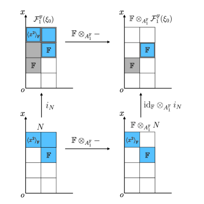
Figure 6: Illustration of 3.32.

Example 3.32.

This example is illustrated in Figures 6 and 7. Let $n=1$. We have $A_{1}^{\mathbb{F}}=\mathbb{F}[x]$. Consider

$$\xi_{0} =\{(1,1),(2,1)\},$$

$$\xi_{1} =\{(2,1),(3,1)\}$$

and define

$$L :=\braket{(x,0),(0,x)}_{\mathbb{F}[x]}\subseteq\mathbb{F}[x](1)\oplus\mathbb{F}[x](2)=\mathcal{F}^{\mathbb{F}}_{1}(\xi_{0}),$$

$$N :=\braket{(x^{2},0),(0,1)}_{\mathbb{F}[x]}\subseteq\mathbb{F}[x](1)\oplus\mathbb{F}[x](2)=\mathcal{F}^{\mathbb{F}}_{1}(\xi_{0}).$$

$L$ and $N$ are graded submodules of $\mathcal{F}_{1}^{\mathbb{F}}(\xi_{0})$. Moreover, $L$ and $N$ are free as an $\mathbb{F}[x]$-modules since $\mathbb{F}[x]$ is principal ideal domain. Hence, they are graded free as $\mathbb{F}[x]$-modules by 3.19. We have $L_{2}=\braket{(x,0)}_{\mathbb{F}}$ and $L_{3}=\braket{(x^{2},0),(0,x)}_{\mathbb{F}}$ which means that the basis elements of $L$ are located in degree $2$ and $3$. Similary $N_{2}=\braket{(0,1)}_{\mathbb{F}}$ and $N_{3}=\braket{(x^{2},0),(0,x)}_{\mathbb{F}}$ and we see that the basis elements of $N$ are also located in degree $2$ and $3$. So, we obtain graded isomorphisms

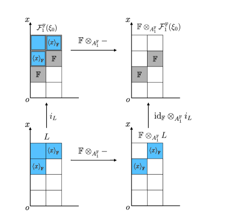
Figure 7: Illustration of 3.32.

$$p_{L}:\mathbb{F}[x](2)\oplus\mathbb{F}[x](3)\longrightarrow L, \quad(0,1)\longmapsto(0,x)$$

$$\quad(1,0)\longmapsto(x,0)$$

$$p_{N}:\mathbb{F}[x](2)\oplus\mathbb{F}[x](3)\longrightarrow N, \quad(1,0)\longmapsto(0,1)$$

$$\quad(0,1)\longmapsto(x^{2},0)$$

which shows that $\Xi^{\mathbb{F}}_{1,0}(L)=\Xi^{\mathbb{F}}_{1,0}(N)=\xi_{1}$. As we can see,

$$\mathcal{F}^{\mathbb{F}}_{1}(\xi_{0})/L\cong\mathbb{F}(3)\oplus\mathbb{F}(2).$$

Hence, $\Xi^{\mathbb{F}}_{1,0}(\mathcal{F}^{\mathbb{F}}_{1}(\xi_{0})/L)=\xi_{0}$. But

$$\mathcal{F}^{\mathbb{F}}_{1}(\xi_{0})/N\cong\mathbb{F}[x]/\braket{x^{2}}(1).$$

So,

$$\Xi^{\mathbb{F}}_{1,0}\left(\mathcal{F}^{\mathbb{F}}_{1}(\xi_{0})/N\right)=\Xi^{\mathbb{F}}_{1,0}\left(\mathbb{F}[x]/\braket{x^{2}}(1)\right)=\{(1,1)\}\neq\xi_{0}.$$

The reason is that $L$ satisfies the tensor-condition by 3.31 while $N$ does not. Moreover, we see that $\xi_{1}\succ_{D}\xi_{0}$ does not hold but $S_{1}^{\mathbb{F}}(\xi_{0},\xi_{1})$ is still non-empty.

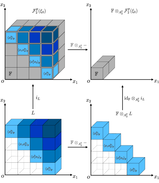
Figure 8: Illustration of 3.33.

Example 3.33.

This example is illustrated in Figure 8. Consider

$$\xi_{0} =\{{\color[rgb]{0,0,0}((0,0),1),((0,0),2)}\},$$

$$\xi_{1} =\{((3,0),1),((2,1),1),((1,2),1),((0,3),1)\}$$

and

$$L =\braket{(x_{1}^{3},0),(x_{1}^{2}x_{2},0),(x_{1}x_{2}^{2},0),(x_{2}^{3},0)}_{A^{\mathbb{F}}_{2}}\subseteq A^{\mathbb{F}}_{2}\oplus A^{\mathbb{F}}_{2},$$

$$N =\braket{(x_{1}^{3},x_{1}^{3}),(x_{1}^{2}x_{2},0),(x_{1}x_{2}^{2},0),(0,x_{2}^{3})}_{A^{\mathbb{F}}_{2}}\subseteq A^{\mathbb{F}}_{2}\oplus A^{\mathbb{F}}_{2}.$$

We have $\xi_{1}\succ_{D}\xi_{0}$. So, the tensor-condition is satisfied by 3.31 which is illustrated for $L$ in Figure 8. We obtain

$$\boldsymbol{\Xi}_{2}^{\mathbb{F}}\left(\mathcal{F}_{2}^{\mathbb{F}}(\xi_{0})/L\right)=\boldsymbol{\Xi}_{2}^{\mathbb{F}}\left(\mathcal{F}_{2}^{\mathbb{F}}(\xi_{0})/N\right)=(\xi_{0},\xi_{1}).$$

Hence, $L,N\in S_{2}^{\mathbb{F}}(\xi_{0},\xi_{1})$. But $\mathcal{F}_{2}^{\mathbb{F}}(\xi_{0})/L$ has elements without $A_{2}^{\mathbb{F}}$-torsion and in $\mathcal{F}_{2}^{\mathbb{F}}(\xi_{0})/N$ every element has $A_{2}^{\mathbb{F}}$-torsion which shows that they are not isomorphic as $A_{2}^{\mathbb{F}}$-modules and therefore not as $n$-graded $A_{2}^{\mathbb{F}}$-modules. So, $\boldsymbol{\Xi}_{2}^{\mathbb{F}}$ is not complete. The multisets $\xi_{0}$ and $\xi_{1}$ will also appear later in Section 4.4 where we follow [CZ07, Sec. 5.2] and [CZ09, Sec. 5.2].

Proof of 3.31.

Assume that for $v\in V_{0}\cap V_{1}$, $\pi_{v}(L_{v})=0$. Let

$$\sum_{j=1}^{l}a_{j}\otimes y_{j}\in\mathrm{im}\left(\mathrm{id}_{\mathbb{F}}\otimes_{A_{n}^{\mathbb{F}}}i_{L}\right).$$

It suffices to show that $a_{j}\otimes y_{j}=0$ for all $j\in\{1,\dots,l\}$. So, let $j\in\{1,\dots,l\}$ and set $a:=a_{j}$ and $y:=y_{j}$. Then

$$y=\sum_{v\in{\mathbb{N}^{n}}}y_{v}\in\bigoplus_{v\in{\mathbb{N}^{n}}}L_{v}\subseteq\mathcal{F}_{n}^{\mathbb{F}}(\xi_{0}).$$

Recall that we have a graded isomorphism

$$\mathbb{F}\otimes_{A_{n}^{\mathbb{F}}}\mathcal{F}_{n}^{\mathbb{F}}(\xi_{0})\xlongrightarrow{\sim}\mathcal{V}_{n}^{\mathbb{F}}(\xi_{0})$$ (10)

of $n$-graded $\mathbb{F}$-vector spaces. Hence, $a\otimes y_{v}=0$ for all $v\in{\mathbb{N}^{n}}\setminus V_{0}$. It remains to show that $a\otimes y_{v}=0$ for all $v\in V_{0}$. Let $v\in V_{0}$. As the generators of $L$ are located in $\bigcup_{v\in V_{1}}L_{v}$, it suffices to show that $a\otimes y_{v}=0$ for all $v\in V_{0}\cap V_{1}$. Let $v\in V_{0}\cap V_{1}$. We have

$$y_{v}\in L_{v}\subseteq\mathcal{F}_{n}^{\mathbb{F}}(\xi)_{v}=\bigoplus_{w\in V_{0}}A_{n}^{\mathbb{F}}(w)^{\mu(w)}_{v}.$$

$y_{v}$ is of the form

$$y_{v}=((z^{(w)}_{1},\dots,z^{(w)}_{\mu(w)}))_{w\in V_{0}}$$

where for $w\prec v$, $z^{(w)}_{i}=\lambda^{(w)}_{i}x^{v-w}$ for suitable $\lambda^{(w)}_{i}\in\mathbb{F}$ and $z^{(w)}_{i}=0$ if $w\npreceq v$. If $v=w$ we have $z^{(v)}_{i}=0$ since $\pi_{v}(L_{v})=0$ by assumption. Enumerate $V_{0}=\{w_{1},\dots,w_{k}\}$ and identify

$$\mathcal{F}_{n}^{\mathbb{F}}(\xi)_{v}=\bigoplus_{w\in V_{0}}A_{n}^{\mathbb{F}}(w)^{\mu(w)}_{v}=\bigoplus_{j=1}^{k}A_{n}^{\mathbb{F}}(w_{j})^{\mu(w_{j})}_{v}$$

along this enumeration. Let $j\in\{1,\dots,k\}$. If $w_{j}\npreceq v$ set $\widetilde{z}^{(w_{j})}_{i}:=z^{(w_{j})}_{i}=0$ for all $i\in\{1,\dots,\mu_{0}(w_{j})\}$ and $x^{v-w_{j}}:=0$. If $w_{j}\preceq v$ set $\widetilde{z}^{(w_{j})}_{i}:=\lambda^{(w_{j})}_{i}$ for all $i\in\{1,\dots,\mu_{0}(w_{j})\}$. By definition of the $A_{n}^{\mathbb{F}}$-module structure on $\mathbb{F}$, we obtain

$$a\otimes y_{v}=a\otimes((z^{(w_{1})}_{1},\dots,z^{(w_{1})}_{\mu(w_{1})}),\dots,(z^{(w_{k})}_{1},\dots,z^{(w_{k})}_{\mu(w_{k})}))$$

$$=\sum_{j=1}^{k}a\otimes((0,\dots,0),\dots,(0,\dots,0),\underset{j}{({z}^{(w_{j})}_{1},\dots,{z}^{(w_{j})}_{\mu(w_{j})})},(0,\dots,0),\dots,(0,\dots,0))$$

$$=\sum_{j=1}^{k}a\cdot x^{v-w_{j}}\otimes((0,\dots,0),\dots,(0,\dots,0),\underset{j}{(\widetilde{z}^{(w_{j})}_{1},\dots,\widetilde{z}^{(w_{j})}_{\mu(w_{j})})},(0,\dots,0),\dots,(0,\dots,0))$$

$$=\sum_{j=1}^{k}0\otimes((0,\dots,0),\dots,(0,\dots,0),\underset{j}{(\widetilde{z}^{(w_{j})}_{1},\dots,\widetilde{z}^{(w_{j})}_{\mu(w_{j})})},(0,\dots,0),\dots,(0,\dots,0))=0.$$

Assume that $\mathrm{id}_{\mathbb{F}}\otimes_{A_{n}^{\mathbb{F}}}i_{L}:\mathbb{F}\otimes_{A_{n}^{\mathbb{F}}}L\to\mathbb{F}\otimes_{A_{n}^{\mathbb{F}}}\mathcal{F}_{n}^{\mathbb{F}}(\xi_{0})$ is the zero map. Let $v\in V_{0}\cap V_{1}$ and $y\in L_{v}$. We can write

$$y=((z^{(w)}_{1},\dots,z^{(w)}_{\mu_{0}(w)}))_{w\in V_{0}}\in\mathcal{F}_{n}^{\mathbb{F}}(\xi_{0})_{v}=\bigoplus_{w\in V_{0}}A_{n}^{\mathbb{F}}(w)_{v}^{\mu_{0}(w)}$$

where $z^{(w)}_{i}\in\mathbb{F}$ if $w=v$. We have $1\otimes y=0$ in $\mathbb{F}\otimes_{A_{n}^{\mathbb{F}}}\mathcal{F}_{n}^{\mathbb{F}}(\xi_{0})_{v}$ by assumption. So, if $v=w$, then necessarily $z^{(w)}_{i}=0$ for all $i\in\{1,\dots,\mu_{0}(w)\}$. ∎

3.5 One-dimensional persistence

Let $n=1$. Recall that $A_{1}^{\mathbb{F}}=\mathbb{F}[x]$. For the following, let $\xi_{0}=(V_{0},\mu_{0})$ and ${\xi_{1}=(V_{1},\mu_{1})}$ be two one-dimensional multisets. The following material about one-dimensional persistence is very common (see for example [CZ05]). Let $[M]\in I_{1}^{\mathbb{F}}(\xi_{0},\xi_{1})$. The the structure theorem (see for example [CZ05, Thm. 2.1] (our notation is different)), states that

$$M\cong\bigoplus_{i=1}^{m}\bigoplus_{j=1}^{d_{i}}\mathbb{F}[x]/\braket{x^{t_{i,j}}}_{\mathbb{F}[x]}(v_{i,j})\oplus\bigoplus_{i=m+1}^{r}\bigoplus_{j=1}^{d_{i}}\mathbb{F}[x](v_{i,j})$$ (11)

as one-graded $\mathbb{F}[x]$-modules for unique $r,m\in\mathbb{N}$ with $r\leq m$ and unique ${d_{i},t_{i,j},v_{i,j}\in\mathbb{N}}$ with $v_{i,j}=v_{i,k}$ for all $j,k\in\{1,\dots,d_{i}\}$. Note that we generally do not have $t_{i,j}=t_{i,k}$ for all $j,k\in\{1,\dots,d_{i}\}$. Using the graded isomorphism in (11), we may define a finite multiset $B_{1}^{\mathbb{F}}(\xi_{0},\xi_{1})([M])$ via

$$B_{1}^{\mathbb{F}}(\xi_{0},\xi_{1})([M]):=\bigcup_{i=1}^{m}\bigcup_{j=1}^{d_{i}}\{([v_{i,j},v_{i,j}+t_{i,j}),j)\}\cup\bigcup_{i=m+1}^{r}\bigcup_{j=1}^{d_{i}}\{([v_{i,j},\infty),j)\}$$

where for $v\in\mathbb{R}$ and $t\in\mathbb{R}\cup\{\infty\}$ with $v<t$, $[v,t)\subseteq\mathbb{R}$ denotes a half-open interval. $B_{1}^{\mathbb{F}}(\xi_{0},\xi_{1})([M])$ is called the barcode of $[M]$ over $(\xi_{0},\xi_{1})$. We have

$$\xi_{0}=\bigcup_{i=1}^{r}\{(v_{i,1},1),\dots,(v_{i,d_{i}},d_{i})\}$$

and

$$\xi_{1}=\bigcup_{i=1}^{m^{\prime}}\{(v^{\prime}_{i,1}+t^{\prime}_{i,1},1),\dots,(v^{\prime}_{i,d^{\prime}_{i}}+t^{\prime}_{i,d^{\prime}_{i}},d^{\prime}_{i})\}.$$

where $v^{\prime}_{i,j}=v_{l,k}$ and $t^{\prime}_{i,j}=t_{l,k}$ after renumbering the $t_{i,j}$ and $v_{i,j}$ according to the multiplicity of the $t_{i,j}$, such that $t_{i,j}=t_{i,k}$ for all $j,k\in\{1,\dots,d^{\prime}_{i}\}$ and ${\sum_{i=1}^{m^{\prime}}d^{\prime}_{i}=\sum_{i=1}^{m}d_{i}}$. As we can see, $\xi_{0}$ and $\xi_{1}$ correspond to the start and end points of elements in $B_{1}^{\mathbb{F}}(\xi_{0},\xi_{1})([M])$. The intuitive interpretation of the barcode is that it captures the lifetime-length of homogeneous generators of $M$.

Example 3.34.

Figure 9 illustrates the barcode

$$\{([0,\infty),1),([0,2),1),([0,1),1),([1,\infty),1),([1,3),1),([1,3),2),([2,3),1),([2,3),2)\}.$$

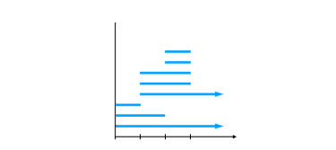
Figure 9: barcode diagram (illustration of 3.34).

Now define $\mathcal{B}(\xi_{0},\xi_{1})$ as the set of all mulitsets

$$\bigcup_{i=1}^{m}\bigcup_{j=1}^{d_{i}}\{([v_{i,j},w_{i,j}),j)\}\cup\bigcup_{i=m+1}^{r}\bigcup_{j=1}^{d_{i}}\{([v_{i,j},\infty),j)\}$$

such that $v_{i,j}<w_{i,j}$,

$$\xi_{0}=\bigcup_{i=1}^{r}\{(v_{i,1},1),\dots,(v_{i,d_{i}},d_{i})\}$$

and

$$\xi_{1}=\bigcup_{i=1}^{m^{\prime}}\{(w^{\prime}_{i,1},1),\dots,(w^{\prime}_{i,d^{\prime}_{i}},d^{\prime}_{i})\}$$

where $w^{\prime}_{i,j}=w_{l,k}$ after renumbering the $w_{l,k}$ according to their multiplicity, such that $w^{\prime}_{i,j}=w^{\prime}_{i,k}$ for all $j,k\in\{1,\dots,d^{\prime}_{i}\}$ and $\sum_{i=1}^{m^{\prime}}d^{\prime}_{i}=\sum_{i=1}^{m}d_{i}$. $\mathcal{B}(\xi_{0},\xi_{1})$ is called the space of barcodes over $(\xi_{0},\xi_{1})$ and

$$\mathcal{B}:=\bigsqcup_{(\xi_{0},\xi_{1})\in\mathcal{T}_{1}}\mathcal{B}(\xi_{0},\xi_{1})$$

is called the space of barcodes. We obtain a set theoretic bijection

$$B_{1}^{\mathbb{F}}(\xi_{0},\xi_{1}):I_{1}^{\mathbb{F}}(\xi_{0},\xi_{1})\xlongrightarrow{\sim}\mathcal{B}(\xi_{0},\xi_{1}),\quad[M]\longmapsto B_{1}^{\mathbb{F}}(\xi_{0},\xi_{1})([M])$$

and $\{B_{1}^{\mathbb{F}}(\xi_{0},\xi_{1})\}_{\mathbb{F}\in\mathcal{K}}$ defines a discrete class of complete invariants. Since

$$\mathbf{Grf}_{1}(A_{1}^{\mathbb{F}})/_{\cong}=\bigsqcup_{(\xi_{0},\xi_{1})\in\mathcal{T}_{1}}I_{1}^{\mathbb{F}}(\xi_{0},\xi_{1})$$

we obtain a set theoretic bijection

$$B^{\mathbb{F}}_{1}:\mathbf{Grf}_{1}(\mathbb{F}[x])/_{\cong}\xlongrightarrow{\sim}\mathcal{B}$$

and $\{B_{1}^{\mathbb{F}}\}_{\mathbb{F}\in\mathcal{K}}$ defines a discrete class of complete invariants, the so-called barcode. We have $\{B_{1}^{\mathbb{F}}\}_{\mathbb{F}\in\mathcal{K}}\cong\{\mathfrak{J}_{1}^{\mathbb{F}}\}_{\mathbb{F}\in\mathcal{K}}$ by 2.20. So, $\{\mathfrak{J}_{1}^{\mathbb{F}}\}_{\mathbb{F}\in\mathcal{K}}$ is a complete class of discrete invariants.

Now one might ask the question if there are barcode-like invariants $B^{\mathbb{F}}_{n}$ for $n\geq 2$ that are equivalent to $\mathfrak{J}^{\mathbb{F}}_{n}$. If $n\geq 2$ it is unfortunately not possible to find a class of invariants $\{f_{n}^{\mathbb{F}}:\mathbf{Grf}_{n}(A_{n}^{\mathbb{F}})\to Q_{n}^{\mathbb{F}}\}_{\mathbb{F}\in\mathcal{K}}$, which is discrete and complete. This is one of the main results in Section 4. In the next section, we present a discrete generalization of the barcode to dimension $n\geq 2$, the so called rank invariant.

3.6 The rank invariant

This section is based on [CZ07, Sec. 6] and [CZ09, Sec. 6]. Let

$$\mathbb{D}^{n}:=\{(u,v)\mid u\in\mathbb{N}^{n},\,v\in{\mathbb{N}^{n}},\,u\preceq v\}\subseteq\mathbb{N}^{n}\times{\mathbb{N}^{n}}$$

be the subset above the diagonal.

Definition 3.35 (Rank invariant).

The assignment

$$\rho_{n}^{\mathbb{F}}:\mathbf{Grf}_{n}(A_{n}^{\mathbb{F}})/_{\cong} \longrightarrow\mathrm{Hom}_{\mathrm{Sets}}(\mathbb{D}^{n},\mathbb{N}^{2}),$$

$$[M] \longmapsto\left(\mathbb{D}^{n}\longrightarrow\mathbb{N}^{2},\,\,(u,v)\longmapsto\left(\mathrm{rank}(x^{v-u}:M_{u}\to M_{v}),\mathrm{dim}_{\mathbb{F}}(M_{u})\right)\right)$$

defines a discrete class of invariants $\{\rho_{n}^{\mathbb{F}}\}_{\mathbb{F}\in\mathcal{K}}$, the so-called rank invariant. Note that $\mathrm{Hom}_{\mathrm{Sets}}(\mathbb{D}^{n},\mathbb{N}^{2})$ is uncountable, but $\mathrm{im}(\rho_{n}^{\mathbb{F}})$ is countable.

Note that in comparison to [CZ09] and [CZ07] our definition of the rank invariant does not map the value $(u,\infty)$. This is not a problem as our definition of the rank invariant already captures all of the information we want to capture. In addition to [CZ09] and [CZ07], we also include the dimension in each degree. The next theorem is from [CZ09, Thm. 12] and [CZ07, Thm. 5] where we use our definition of the rank invariant.

Theorem 3.36 ([CZ09, Thm. 12], [CZ07, Thm. 5]).

We have $\{\rho_{1}^{\mathbb{F}}\}_{\mathbb{F}\in\mathcal{K}}\cong\{B_{1}^{\mathbb{F}}\}_{\mathbb{F}\in\mathcal{K}}$ which shows that $\{\rho_{1}^{\mathbb{F}}\}_{\mathbb{F}\in\mathcal{K}}$ is complete.

Sketch of the proof.

As in [CZ07, Thm. 5] and [CZ09, Thm. 12], the idea is to show that the assignment

$$\mathcal{B}\longrightarrow\mathrm{im}\left(\rho_{1}^{\mathbb{F}}\right),$$

which sends a barcode $B\in\mathcal{B}$ to the function

$$\mathbb{D}^{1} \longrightarrow\mathbb{N}^{2},$$

$$(u,v) \longmapsto\left(\left|\left\{([t,s),i)\in B\mid[u,v)\subseteq[t,s)\right\}\right|,\left|\left\{([t,s),i)\in B\mid u\in[t,s)\right\}\right|\right),$$ (12)

is a bijection. Our proof goes a different way than the proof in [CZ07] and [CZ09].

The idea is as follows: for $u,v\in{\mathbb{N}}$ with $u\leq v$, we have

$$\mathrm{dim}_{\mathbb{F}}(\mathrm{ker}(M_{u}\to M_{v}))=\mathrm{dim}_{\mathbb{F}}(M_{u})-\mathrm{rank}(M_{u}\to M_{v})$$ (13)

which corresponds to the number of homogeneous generators in $M_{u}$ whose lifetime end in $M_{v}$. Using this formula, we may simply read off the rank invariant from a given barcode as described in (3.6) and the assignment is clearly well-defined and injective. The intuition for surjectivity is as follows: let $C\in\mathrm{im}(\rho_{1}^{\mathbb{F}})$. Then $C=\rho_{1}^{\mathbb{F}}([M])$ for some $[M]\in\mathbf{Grf}_{1}(\mathbb{F}[x])/_{\cong}$. Let $(u,v)\in\mathbb{D}^{1}=\{(u,v)\in{\mathbb{N}}^{2}\mid u\leq v\}$. We know that $B(\psi_{M})$ exists. The question is how $B(\psi_{M})$ is determined by $\rho_{1}^{\mathbb{F}}([M])$. Using (13), we see that $\rho_{1}^{\mathbb{F}}([M])$ gives us all the information about the lifetime length of homogeneous generators for each $M_{v}$ with $v\in{\mathbb{N}}$. So, the shape of $B(\psi_{M})$ is determined as follows: we start in $M_{0}$ and determine the lifetime length of each homogeneous generator via (13). Then we do the same for $M_{1}$ and so on. This procedure terminates, since for some $\alpha\in{\mathbb{N}}$, $M_{\alpha}\to M_{v}$ has to be an isomorphism of $\mathbb{F}$-vector spaces for all $v\in\mathbb{N}_{\geq\alpha}$ (see [CZ05, Def. 3.3, Thm. 3.1]). ∎

So, $\{\rho_{n}^{\mathbb{F}}\}_{\mathbb{F}\in\mathcal{K}}$ is a discrete generalization of $\{B_{1}^{\mathbb{F}}\}_{\mathbb{F}\in\mathcal{K}}$ to dimension $n\geq 2$.

4 Parameterization

The first goal of this section is to show that for $n\geq 2$, there exists no class

$$\left\{f_{n}^{\mathbb{F}}:\mathbf{Grf}_{n}(A_{n}^{\mathbb{F}})/_{\cong}\longrightarrow Q_{n}^{\mathbb{F}}\right\}_{\mathbb{F}\in\mathcal{K}}$$

of invariants which is complete and discrete. As $\{\mathfrak{J}_{n}^{\mathbb{F}}\}_{\mathbb{F}\in\mathcal{K}}$ is complete, it suffices to show that $\{\mathfrak{J}_{n}^{\mathbb{F}}\}_{\mathbb{F}\in\mathcal{K}}$ is not discrete for $n\geq 2$ by 2.20. Let $\xi_{0}$ and $\xi_{1}$ be two finite $n$-dimensional multisets. In Sections 4.1-4.3, we parameterize $S_{n}^{\mathbb{F}}(\xi_{0},\xi_{1})$ as a subset of a product of Grassmannians together with a group action of ${\mathrm{Aut}(\mathcal{F}_{n}^{\mathbb{F}}(\xi_{0}))}$. This approach follows [CZ07, Sec. 4.3] and [CZ09, Sec. 5]. However, the authors ommited proofs and details. We fill in the gaps and give detailed proofs. Using this parameterization, we show the non-existence of a discrete and complete class of invariants in Section 4.4.

In Section 4.5, we investigate the second goal of this section: that this subset corresponds to the set of $\mathbb{F}$-points of an algebraic variety together with an algebraic group action of ${\mathrm{Aut}(\mathcal{F}_{n}^{\mathbb{F}}(\xi_{0}))}$. In other words, we want to give an explicit parameterization of the moduli space of our classification problem. Here we follow [CZ07, Sec. 5] and [CZ09, Sec. 5]. In Section 4.5.1, we construct a subprevariety $\mathcal{Y}_{n}^{\mathbb{F}}(\xi_{0},\xi_{1})$ of a product of Grassmann varieties (over $\mathbb{F}$) such that

$$\mathcal{Y}_{n}^{\mathbb{F}}(\xi_{0},\xi_{1})(\mathbb{F})\cong S_{n}^{\mathbb{F}}(\xi_{0},\xi_{1}).$$

$\mathrm{GL}_{m}(\mathbb{F})$ can be realized as the set of $\mathbb{F}$-points of an affine algebraic group $\mathcal{GL}_{m}^{\mathbb{F}}$ over $\mathbb{F}$. Now it is possible to show that $\mathrm{Aut}(\mathcal{F}_{n}^{\mathbb{F}}(\xi_{0}))$ corresponds to the set of $\mathbb{F}$-points of a closed subscheme

$$\mathcal{GL}_{\preceq}^{\mathbb{F}}(\xi_{0})\subseteq\mathcal{GL}_{m_{0}}^{\mathbb{F}}$$

where $m_{0}:=\left\lvert\xi_{0}\right\lvert$. Assuming that $\mathcal{GL}_{\preceq}^{\mathbb{F}}(\xi_{0})$ is an algebraic group, the idea is now (using the functor of points approach) to define for every Noetherian $\mathbb{F}$-algebra $T$ a group action

$$\mathcal{GL}_{\preceq}^{\mathbb{F}}(\xi_{0})(T)\times\mathcal{Y}_{n}^{\mathbb{F}}(\xi_{0},\xi_{1})(T)\longrightarrow\mathcal{Y}_{n}^{\mathbb{F}}(\xi_{0},\xi_{1})(T)$$

which is natural in $T$. For this, we have to determine the $T$-points $\mathcal{GL}_{\preceq}^{\mathbb{F}}(\xi_{0})(T)$ and $\mathcal{Y}_{n}^{\mathbb{F}}(\xi_{0},\xi_{1})(T)$. For $\mathcal{GL}_{\preceq}^{\mathbb{F}}(\xi_{0})(T)$ this is not difficult, but for $\mathcal{Y}_{n}^{\mathbb{F}}(\xi_{0},\xi_{1})(T)$ it is. In Section 4.5.2, we give some ideas that provide evidence for how this can be done. For Grassmann varieties (and therefore also for products of Grassmann varieties) this problem is also technical but solved (see for instance [GW10, (8.4)]). Since $\mathcal{Y}_{n}^{\mathbb{F}}(\xi_{0},\xi_{1})$ is constructed as a subprevariety of a product of Grassmann varieties, we use the approach for Grassmann varieties. In [CZ09, Sec. 5], the authors give a proof for the subprevariety-part which does not contain an interpretation of the tensor-condition in terms of polynomial equations. In [CZ07, Thm. 4], the subprevariety-part is stated where in comparison to [CZ09, Sec. 5] a proof and conditions are missing. In [CZ07, Thm. 4] and [CZ09, Sec. 5], the authors claim (without a proof) that the action is algebraic.

4.1 Relation families

For the following let $\xi_{0}=(V_{0},\mu_{0})$ and $\xi_{1}=(V_{1},\mu_{1})$ be two finite $n$-dimensional multisets such that $S_{n}^{\mathbb{F}}(\xi_{0},\xi_{1})$ is non-empty. In this section, we start with the parameterization of $S_{n}^{\mathbb{F}}(\xi_{0},\xi_{1})/\mathrm{Aut}(\mathcal{F}_{n}^{\mathbb{F}}(\xi_{0}))$. The idea is to map $L\in S_{n}^{\mathbb{F}}(\xi_{0},\xi_{1})$ to the corresponding familiy of $\mathbb{F}$-vector spaces $(L_{w})_{w\in V_{1}}$ and to determine the conditions under which such a family of $\mathbb{F}$-vector spaces yields an element in $S_{n}^{\mathbb{F}}(\xi_{0},\xi_{1})$. These conditions are given in the next definition.

Definition 4.1 ($\mathbb{F}$-relation family).

An $\mathbb{F}$-relation family with respect to $(\xi_{0},\xi_{1})$ is a family $(L_{w})_{w\in V_{1}}$ such that for all $w\in V_{1}$:

1. $L_{w}\subseteq\mathcal{F}_{n}^{\mathbb{F}}(\xi_{0})_{w}$ is an $\mathbb{F}$-linear subspace.

2. $\mathrm{dim}_{\mathbb{F}}(L_{w})=\mathrm{dim}_{\mathbb{F}}\left(\mathcal{F}_{n}^{\mathbb{F}}(\xi_{1})_{w}\right)$.

3. if $v\in V_{1}$ with $v\prec w$, then $x^{w-v}L_{v}\subseteq L_{w}$.

4. if $w\in V_{0}\cap V_{1}$, then we have $\pi_{w}(L_{w})=0$ where $\pi_{w}:\mathcal{F}_{n}^{\mathbb{F}}(\xi_{0})_{w}\to A_{n}^{\mathbb{F}}(w)^{\mu_{0}(w)}_{w}$ denotes the canonical projection. Note that $A_{n}^{\mathbb{F}}(w)^{\mu_{0}(w)}_{w}=\mathbb{F}^{\mu_{0}(w)}$.

5. $\mathrm{dim}_{\mathbb{F}}\left(L_{w}/\sum_{v\prec w}x^{w-v}L_{v}\right)=\mu_{1}(w)$.

$R_{n}^{\mathbb{F}}(\xi_{0},\xi_{1})$ denotes the set of all $\mathbb{F}$-relation families with respect to $(\xi_{0},\xi_{1})$.

Our definition of $\mathbb{F}$-relation families is based on [CZ07, Def. 9] and [CZ09, Sec. 5, p. 85]. [CZ09] is more general than [CZ07, Def. 9] and has $5$ as an extra condition, but condition $4$ is missing. In [CZ07], conditions $4$ and $5$ are missing. The next theorem is based on and inspired by [CZ07, Thm. 3] and [CZ09, Sec. 5]. Both articles do not give a proof.

Theorem 4.2.

The map

$$\varphi_{n}^{\mathbb{F}}(\xi_{0},\xi_{1}):S_{n}^{\mathbb{F}}(\xi_{0},\xi_{1})\xlongrightarrow{\sim}R_{n}^{\mathbb{F}}(\xi_{0},\xi_{1}),\quad L\longmapsto(L_{w})_{w\in V_{1}}$$

is a set theoretic bijection with inverse

$$\phi_{n}^{\mathbb{F}}(\xi_{0},\xi_{1}):R_{n}^{\mathbb{F}}(\xi_{0},\xi_{1})\xlongrightarrow{\sim}S_{n}^{\mathbb{F}}(\xi_{0},\xi_{1}),\quad(L_{w})_{w\in V_{1}}\longmapsto\left\langle\bigcup_{w\in V_{1}}L_{w}\right\rangle_{A_{n}^{\mathbb{F}}}.$$

Before we proceed with a proof of 4.2, we give two examples for $\mathbb{F}$-relation families:

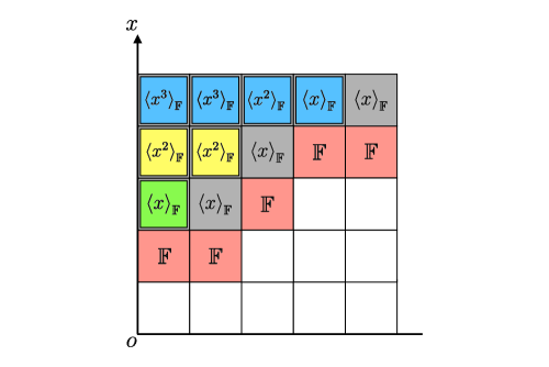
Figure 10: $\mathbb{F}$-relation family in dimension $n=1$ (illustration of 4.3).

Example 4.3.

Let $n=1$. Consider

$$\xi_{0} :=\{(1,1),(1,2),(2,1),(3,1),(3,2)\}$$

$$\xi_{1} :=\{(2,1),(3,1),(4,1),(4,2)\}$$

and let

$$L_{4} :=\left\langle(x^{3},0,0,0,0),(0,x^{3},0,0,0),(0,0,x^{2},0,0),(0,0,0,x,0)\right\rangle_{\mathbb{F}}\subseteq\mathcal{F}_{1}^{\mathbb{F}}(\xi_{0})_{4},$$

$$L_{3} :=\left\langle(x^{2},0,0,0,0),(0,x^{2},0,0,0)\right\rangle_{\mathbb{F}}\subseteq\mathcal{F}_{1}^{\mathbb{F}}(\xi_{0})_{3},$$

$$L_{2} :=\left\langle(x,0,0,0,0)\right\rangle_{\mathbb{F}}\subseteq\mathcal{F}_{1}^{\mathbb{F}}(\xi_{0})_{2}.$$

Then $(L_{j})_{j\in\{2,3,4\}}\in R_{1}^{\mathbb{F}}(\xi_{0},\xi_{1})$. Figure 10 illustrates $(L_{j})_{j\in\{2,3,4\}}$. The blue blocks correspond to $L_{4}$, the yellow blocks correspond to $L_{3}$ and the green block corresponds to $L_{2}$. The red blocks are the "forbidden" blocks that we get from condition $4$ in $R_{1}^{\mathbb{F}}(\xi_{0},\xi_{1})$. By using Theorems 3.29 and 4.2, we obtain a set theoretic bijection

$$R_{1}^{\mathbb{F}}(\xi_{0},\xi_{1})/\mathrm{Aut}(\mathcal{F}_{1}^{\mathbb{F}}(\xi_{0})\cong I_{1}^{\mathbb{F}}(\xi_{0},\xi_{1}).$$

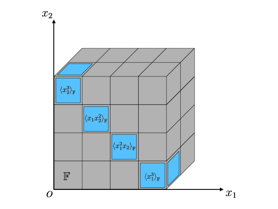
Figure 11: $\mathbb{F}$-relation family in dimension $n=2$ (illustration of 4.4).

Example 4.4.

This example can be found in [CZ07, Sec. 5.2], [CZ09, Sec. 5.2] and will be also discussed later in Section 4.4. Let $n=2$. As in 3.33, consider

$$\xi_{0} :=\{{\color[rgb]{0,0,0}((0,0),1),((0,0),2)}\},$$

$$\xi_{1} :=\{((3,0),1),((2,1),1),((1,2),1),((0,3),1)\}.$$

Then conditions 3-5 in $R_{2}^{\mathbb{F}}(\xi_{0},\xi_{1})$ are trivial and we obtain

$$R_{2}^{\mathbb{F}}(\xi_{0},\xi_{1})=\prod_{w\in V_{1}}\left\{L_{w}\subseteq\mathcal{F}_{2}^{\mathbb{F}}(\xi_{0})_{w}\mid\mathrm{dim}_{\mathbb{F}}(L_{w})=\mathrm{dim}_{\mathbb{F}}\left(\mathcal{F}_{2}^{\mathbb{F}}(\xi_{1})_{w}\right)=1\right\}$$

Since $\mathcal{F}_{2}^{\mathbb{F}}(\xi_{0})_{w}\cong\mathbb{F}^{2}$ for all $w\in V_{1}$, we have

$$R_{2}^{\mathbb{F}}(\xi_{0},\xi_{1})\cong\mathbb{P}_{1}(\mathbb{F})^{4}$$

as sets, where $\mathbb{P}_{1}(\mathbb{F})$ denotes the projective line over $\mathbb{F}$ (i.e. the set of all one-dimensional subspaces of $\mathbb{F}^{2}$). Figure 11 illustrates $(L_{w})_{w\in V_{1}}\in R_{2}^{\mathbb{F}}(\xi_{0},\xi_{1})$ where

$$L_{(3,0)}:=\braket{(x_{1}^{3},0)}_{\mathbb{F}}\subseteq\mathcal{F}_{2}^{\mathbb{F}}(\xi_{0})_{(3,0)},$$

$$L_{(2,1)}:=\braket{(x_{1}^{2}x_{2},0)}_{\mathbb{F}}\subseteq\mathcal{F}_{2}^{\mathbb{F}}(\xi_{0})_{(2,1)},$$

$$L_{(1,2)}:=\braket{(x_{1}x_{2}^{2},0)}_{\mathbb{F}}\subseteq\mathcal{F}_{2}^{\mathbb{F}}(\xi_{0})_{(1,2)},$$

$$L_{(0,3)}:=\braket{(x_{2}^{3},0)}_{\mathbb{F}}\subseteq\mathcal{F}_{2}^{\mathbb{F}}(\xi_{0})_{(0,3)}.$$

Proof of 4.2.

$\varphi_{n}^{\mathbb{F}}(\xi_{0},\xi_{1})$ is well-defined: let $L\in S_{n}^{\mathbb{F}}(\xi_{0},\xi_{1})$. Since $L$ is graded, condition $1$ and $3$ are satisfied. Condition $4$ is equivalent to the tensor-condition by 3.31. It remains to show that condition $2$ and $5$ are satisfied. Let ${p_{1}:\mathcal{F}_{n}^{\mathbb{F}}(\xi_{1})\to L}$ be a free hull of $L$ and $E_{\xi_{1}}:=\bigcup_{v\in V_{1}}E_{v}$ be the standard basis of $\mathcal{F}_{n}^{\mathbb{F}}(\xi_{1})$ as $A_{n}^{\mathbb{F}}$-module where for $v\in V_{1}$, $E_{v}$ corresponds to the block $A_{n}^{\mathbb{F}}(v)^{\mu_{1}(v)}_{v}=\mathbb{F}^{\mu_{0}(v)}$. Let $w\in V_{1}$ and $E_{v\preceq w}:=\bigcup_{v\preceq w}E_{v}$. Then $\mathcal{F}_{n}^{\mathbb{F}}(\xi_{1})_{w}=\braket{E_{v\preceq w}}_{\mathbb{F}}$ and $p_{1}(E_{\xi_{1}})$ is a minimal set of homogeneous generators of $L$ by 3.20 and $p_{1}(E_{v\preceq w})$ is an $\mathbb{F}$-basis of $L_{w}$. We have

$$p_{1}(\braket{E_{v\preceq w}}_{\mathbb{F}})=p_{1}(\mathcal{F}_{n}^{\mathbb{F}}(\xi_{1})_{w})=L_{w}$$

which shows that $\mathrm{dim}_{\mathbb{F}}(\mathcal{F}_{n}^{\mathbb{F}}(\xi_{1})_{w})\geq\mathrm{dim}_{\mathbb{F}}(L_{w})$ and equality must hold due to minimality. Thus, condition $2$ is satisfied. It remains to show that condition $5$ is satisfied: since $\mathcal{F}_{n}^{\mathbb{F}}(\xi_{0})$ is graded free and $L\subseteq\mathcal{F}_{n}^{\mathbb{F}}(\xi_{0})$ is graded, multiplication by $x^{w-v}$ is an $\mathbb{F}$-vector space monomorphism from $L_{v}$ to $L_{w}$ for all $v,w\in{\mathbb{N}^{n}}$ with $v\preceq w$. Therefore,

$$\mathrm{dim}_{\mathbb{F}}(L_{w}/x^{w-v}L_{v}) =\mathrm{dim}_{\mathbb{F}}(L_{w})-\mathrm{dim}_{\mathbb{F}}(L_{v})=\left\lvert E_{u\preceq w}\right\lvert-\left\lvert E_{u\preceq v}\right\lvert$$

$$=\sum_{u\preceq w}\mu_{1}(u)-\sum_{u\preceq v}\mu_{1}(u)=\sum_{v\prec u\preceq w}\mu_{1}(u).$$

If we procced inductively we see that condition $5$ is satisfied. So, we conlude that $\varphi_{n}^{\mathbb{F}}(\xi_{0},\xi_{1})$ is well-defined.

$\phi_{n}^{\mathbb{F}}(\xi_{0},\xi_{1})$ is well-defined: let $(L_{w})_{w\in V_{1}}\in R_{n}^{\mathbb{F}}(\xi_{0},\xi_{1})$ and

$$L:=\left\langle\bigcup_{w\in V_{1}}L_{w}\right\rangle_{A_{n}^{\mathbb{F}}}\subseteq\mathcal{F}_{n}^{\mathbb{F}}(\xi_{0}).$$

Then $L\subseteq\mathcal{F}_{n}^{\mathbb{F}}(\xi_{0})$ is a graded $A_{n}^{\mathbb{F}}$-submodule since it is generated by homogeneous elements (see 2.13). Condition $4$ is equivalent to the tensor-condition by 3.31. So, it remains to show that $L$ has type $\xi_{1}$:

1. let $V_{1,1}^{\mathrm{max}}\subseteq V_{1}$ be the set of all maximal $v\in V_{1}$ with respect to $\preceq$. Then $\mathrm{dim}_{\mathbb{F}}\left(L_{w}/\sum_{v\prec w}x^{w-v}L_{v}\right)=\mu_{1}(w)$ for all $w\in V_{1,1}^{\mathrm{max}}$. For all $w\in V_{1,1}^{\mathrm{max}}$, let $B_{1,w}\subseteq L_{w}$ with $\left\lvert B_{w}\right\lvert=\mu_{1}(w)$ such that

   $$\left\langle B_{w}\cup\sum_{v\prec w}x^{w-v}L_{v}\right\rangle_{\mathbb{F}}=L_{w}$$

   As $\mathrm{dim}_{\mathbb{F}}(L_{w})=\mathrm{dim}_{\mathbb{F}}\left(\mathcal{F}_{n}^{\mathbb{F}}(\xi_{1})_{w}\right)$ we see that

   $$\mathrm{dim}_{\mathbb{F}}\left(\sum_{v\prec w}x^{w-v}L_{v}\right)=\mathrm{dim}_{\mathbb{F}}\left(\mathcal{F}_{n}^{\mathbb{F}}(\xi_{1})_{w}\right)-\mu_{1}(w)$$

   for all $w\in V_{1,1}^{\mathrm{max}}$.

2. let $V_{2,1}^{\mathrm{max}}\subseteq V_{1}\setminus V_{1,1}^{\mathrm{max}}$ be the set of all maximal $v\in V_{1}\setminus V_{1,1}^{\mathrm{max}}$ with respect to $\preceq$. Then $\mathrm{dim}_{\mathbb{F}}\left(L_{w}/\sum_{v\prec w}x^{w-v}L_{v}\right)=\mu_{1}(w)$ for all $w\in V_{2,1}^{\mathrm{max}}$. For all $w\in V_{2,1}^{\mathrm{max}}$, let $B_{w}\subseteq L_{w}$ with $\left\lvert B_{w}\right\lvert=\mu_{1}(w)$ such that

   $$\left\langle B_{w}\cup\sum_{v\prec w}x^{w-v}L_{v}\right\rangle_{\mathbb{F}}=L_{w}$$

   As $\mathrm{dim}_{\mathbb{F}}(L_{w})=\mathrm{dim}_{\mathbb{F}}\left(\mathcal{F}_{n}^{\mathbb{F}}(\xi_{1})_{w}\right)$ we see that

   $$\mathrm{dim}_{\mathbb{F}}\left(\sum_{v\prec w}x^{w-v}L_{v}\right)=\mathrm{dim}_{\mathbb{F}}\left(\mathcal{F}_{n}^{\mathbb{F}}(\xi_{1})_{w}\right)-\mu_{1}(w)$$

   for all $w\in V_{2,1}^{\mathrm{max}}$.

If we proceed inducutively this way, there exists an $m\in\mathbb{N}$ such that $V_{m,1}^{\mathrm{max}}\neq\emptyset$ and $V_{m+1,1}^{\mathrm{max}}=\emptyset$

1. as $V_{m+1,1}^{\mathrm{max}}=\emptyset$, we have $\mathrm{dim}_{\mathbb{F}}(L_{w})=\mu_{1}(w)$ for all $w\in V_{m,1}^{\mathrm{max}}$. Now let $B_{w}\subseteq L_{w}$ be an $\mathbb{F}$-basis. Then $\left\lvert B_{w}\right\lvert=\mu_{1}(w)=\mathrm{dim}_{\mathbb{F}}(L_{w})$.

By construction, we have

$$L_{w}=\left\langle\bigcup_{v\preceq w}x^{w-v}B_{v}\right\rangle_{\mathbb{F}}.$$ (14)

Since multiplication by $x^{w-v}$ is an $\mathbb{F}$-vector space monomorphism from $\mathcal{F}_{n}^{\mathbb{F}}(\xi_{0})_{v}$ to $\mathcal{F}_{n}^{\mathbb{F}}(\xi_{0})_{w}$, it holds that

$$\left\lvert x^{w-v}B_{v}\right\lvert=\left\lvert B_{v}\right\lvert.$$

So, we have

$$\left\lvert\bigcup_{v\preceq w}x^{w-v}B_{v}\right\lvert \leq\sum_{v\preceq w}\left\lvert x^{w-v}B_{v}\right\lvert=\sum_{v\preceq w}\left\lvert B_{v}\right\lvert$$

$$=\sum_{v\preceq w}\mu_{1}(v)=\mathrm{dim}_{\mathbb{F}}\left(\mathcal{F}_{n}^{\mathbb{F}}(\xi_{1})_{w}\right)=\mathrm{dim}_{\mathbb{F}}(L_{w}).$$ (15)

Now (14) and (4.1) imply that $\bigcup_{v\preceq w}x^{w-v}B_{v}$ is an $\mathbb{F}$-basis of $L_{w}$. Therefore,

$$B:=\bigcup_{v\in V_{1}}B_{v}$$

is a finite system of homogeneous generators of $L$. Note that the union $\bigcup_{v\in V_{1}}B_{v}$ is disjoint since the $B_{v}$ live in different degrees. Since

$$\left\lvert B\right\lvert=\sum_{v\in V_{1}}\mu_{1}(v)=\left\lvert\xi_{1}\right\lvert=\mathrm{dim}_{\mathbb{F}}(\mathbb{F}\otimes_{A_{n}^{\mathbb{F}}}L)=\mathrm{dim}_{\mathbb{F}}(L/\mathfrak{m}_{n}^{\mathbb{F}}L)$$

and since $\pi(B)$ generates $L/\mathfrak{m}_{n}^{\mathbb{F}}L$ (where $\pi:L\to L/\mathfrak{m}_{n}^{\mathbb{F}}L$ denotes the canonical projection), we conclude that $\pi(B)$ is an $\mathbb{F}$-basis of $L/\mathfrak{m}_{n}^{\mathbb{F}}L$. Hence, $B$ is minimal by 3.16.

Recall that $E_{\xi_{1}}=\bigcup_{v\in V_{1}}E_{v}$ is the standard basis of $\mathcal{F}_{n}^{\mathbb{F}}(\xi_{1})$ as an $n$-graded $A_{n}^{\mathbb{F}}$-module. We have $\left\lvert E_{v}\right\lvert=\mu_{1}(v)=\left\lvert B_{v}\right\lvert$. So, there are set theoretic bijections $\iota_{v}:E_{v}\xrightarrow{\sim}B_{v}$. Thus,

$$p_{1}:\mathcal{F}_{n}^{\mathbb{F}}(\xi_{1})\longrightarrow L,\quad E_{v}\ni b\longmapsto\iota_{v}(b)$$

defines a surjective morphism of $n$-graded $A_{n}^{\mathbb{F}}$-modules. Since $B$ is minimal, $(\mathcal{F}_{n}^{\mathbb{F}}(\xi_{1}),p_{1})$ is a free hull of $L$ by 3.20 and $L$ has type $\xi_{1}$.

$\varphi_{n}^{\mathbb{F}}(\xi_{0},\xi_{1})$ and $\phi_{n}^{\mathbb{F}}(\xi_{0},\xi_{1})$ are inverse to each other: Let $L\in S_{n}^{\mathbb{F}}(\xi_{0},\xi_{1})$. Since, $L$ has type $\xi_{1}$ the generators of $L$ are located in $\bigcup_{w\in V_{1}}L_{w}$ and we obtain

$$\phi_{n}^{\mathbb{F}}(\xi_{0},\xi_{1})(\varphi_{n}^{\mathbb{F}}(\xi_{0},\xi_{1})(L))=\phi_{n}^{\mathbb{F}}(\xi_{0},\xi_{1})((L_{w})_{w\in V_{1}})=\left\langle\bigcup_{w\in V_{1}}L_{w}\right\rangle_{A_{n}^{\mathbb{F}}}=L.$$

Now let $(L_{w})_{w\in V_{1}}\in R_{n}^{\mathbb{F}}(\xi_{0},\xi_{1})$ and let

$$N:=\left\langle\bigcup_{w\in V_{1}}L_{w}\right\rangle_{A_{n}^{\mathbb{F}}}.$$

Let $w\in V_{1}$. Then $L_{w}\subseteq N_{w}$. Since $\phi_{n}^{\mathbb{F}}(\xi_{0},\xi_{1})$ is well-defined, we know that $N$ has type $\xi_{1}$. So, there exists a surjective graded $A_{n}^{\mathbb{F}}$-module homomorphism $p_{1}:\mathcal{F}_{n}^{\mathbb{F}}(\xi_{1})\to N$. Since $(L_{w})_{w\in V_{1}}\in R_{n}^{\mathbb{F}}(\xi_{0},\xi_{1})$, we have $\mathrm{dim}_{\mathbb{F}}(\mathcal{F}_{n}^{\mathbb{F}}(\xi_{1})_{w})=\mathrm{dim}_{\mathbb{F}}(L_{w})$. Thus, we obtain

$$\mathrm{dim}_{\mathbb{F}}(L_{w})\leq\mathrm{dim}_{\mathbb{F}}(N_{w})\leq\mathrm{dim}_{\mathbb{F}}(\mathcal{F}_{n}^{\mathbb{F}}(\xi_{1})_{w})=\mathrm{dim}_{\mathbb{F}}(L_{w})$$

which shows that $\mathrm{dim}_{\mathbb{F}}(L_{w})=\mathrm{dim}_{\mathbb{F}}(N_{w})$. Since $L_{w}\subseteq N_{w}$, we have $L_{w}=N_{w}$. Therefore,

$$\varphi_{n}^{\mathbb{F}}(\xi_{0},\xi_{1})(\phi_{n}^{\mathbb{F}}(\xi_{0},\xi_{1})((L_{w})_{w\in V_{1}}))=\varphi_{n}^{\mathbb{F}}(\xi_{0},\xi_{1})(N)=(L_{w})_{w\in V_{1}}.$$

So, $\varphi_{n}^{\mathbb{F}}(\xi_{0},\xi_{1})$ and $\phi_{n}^{\mathbb{F}}(\xi_{0},\xi_{1})$ are inverse to each other ∎

Definition, Proposition 4.5.

$\mathrm{Aut}(\mathcal{F}_{n}^{\mathbb{F}}(\xi_{0}))$ acts as a group on $R_{n}^{\mathbb{F}}(\xi_{0},\xi_{1})$ where for $(L_{w})_{w\in V_{1}}\in R_{n}^{\mathbb{F}}(\xi_{0},\xi_{1})$ and $f\in\mathrm{Aut}(\mathcal{F}_{n}^{\mathbb{F}}(\xi_{0}))$,

$$f\cdot(L_{w})_{w\in V_{1}}:=\left(f(L_{w})\right)_{w\in V_{1}}.$$

Proof.

We have to check that conditions $1$-$5$ in $R_{n}^{\mathbb{F}}(\xi_{0},\xi_{1})$ are preserverd under this action. So, let $(L_{w})_{w\in V_{1}}\in R_{n}^{\mathbb{F}}(\xi_{0},\xi_{1})$ and $f\in\mathrm{Aut}(\mathcal{F}_{n}^{\mathbb{F}}(\xi_{0})$. Then

$$L:=\left\langle\bigcup_{w\in V_{1}}L_{w}\right\rangle_{A_{n}^{\mathbb{F}}}=\varphi_{n}^{\mathbb{F}}(\xi_{0},\xi_{1})((L_{w})_{w\in V_{1}})\in S_{n}^{\mathbb{F}}(\xi_{0},\xi_{1})$$

by 4.2. We have $f(L)\in S_{n}^{\mathbb{F}}(\xi_{0},\xi_{1})$ and since $f$ is a graded automorphism, we have $f(L)_{w}=f(L_{w})$ for all $w\in{\mathbb{N}^{n}}$. Using 4.2, we therefore conclude that

$$(f(L_{w}))_{w\in V_{1}}=(f(L)_{w})_{w\in V_{1}}=\phi_{n}^{\mathbb{F}}(\xi_{0},\xi_{1})(f(L))\in R_{n}^{\mathbb{F}}(\xi_{0},\xi_{1}).$$

∎

Theorem 4.6.

$\varphi_{n}^{\mathbb{F}}(\xi_{0},\xi_{1})$ and $\phi^{\mathbb{F}}(\xi_{0},\xi_{1})$ are $\mathrm{Aut}(\mathcal{F}_{n}^{\mathbb{F}}(\xi_{0}))$-equivariant and they induce mutually inverse set theoretic bijections

$$\overline{\varphi}_{n}^{\mathbb{F}}(\xi_{0},\xi_{1}):S_{n}^{\mathbb{F}}(\xi_{0},\xi_{1})/\mathrm{Aut}(\mathcal{F}_{n}^{\mathbb{F}}(\xi_{0}))\longrightarrow R_{n}^{\mathbb{F}}(\xi_{0},\xi_{1})/\mathrm{Aut}(\mathcal{F}_{n}^{\mathbb{F}}(\xi_{0}))$$

and

$$\overline{\phi}_{n}^{\mathbb{F}}(\xi_{0},\xi_{1}):R_{n}^{\mathbb{F}}(\xi_{0},\xi_{1})/\mathrm{Aut}(\mathcal{F}_{n}^{\mathbb{F}}(\xi_{0}))\longrightarrow S_{n}^{\mathbb{F}}(\xi_{0},\xi_{1})/\mathrm{Aut}(\mathcal{F}_{n}^{\mathbb{F}}(\xi_{0})).$$

Thus,

$$I_{n}^{\mathbb{F}}(\xi_{0},\xi_{1})\cong R_{n}^{\mathbb{F}}(\xi_{0},\xi_{1})/\mathrm{Aut}(\mathcal{F}_{n}^{\mathbb{F}}(\xi_{0}))$$

as sets.

Proof.

Both $\varphi_{n}^{\mathbb{F}}(\xi_{0},\xi_{1})$ and $\phi_{n}^{\mathbb{F}}(\xi_{0},\xi_{1})$ are $\mathrm{Aut}(\mathcal{F}_{n}^{\mathbb{F}}(\xi_{0}))$-equivariant by definition of the $\mathrm{Aut}(\mathcal{F}_{n}^{\mathbb{F}}(\xi_{0}))$-action. The rest is clear by 4.2 and 3.29. ∎

4.2 The automorphism group

Recall that $\xi_{0}=(V_{0},\mu_{0})$ is a finite $n$-dimensional mulitset. In this section, we give an explicit description of $\mathrm{Aut}(\mathcal{F}_{n}^{\mathbb{F}}(\xi_{0}))$ in terms of transformation matrices.

Our next definition, proposition is from [CZ07, Lem. 3] (see also [CZ09, Sec. 4.3]).

Definition, Proposition 4.7.

Define

$$\mathrm{Aut}_{\preceq}^{\mathbb{F}}(\xi_{0})\subseteq\mathrm{Aut}\left(\bigoplus_{v\in V_{0}}\mathbb{F}^{\mu_{0}(v)}\right)$$

as the subgroup of all $\mathbb{F}$-vector space automorphisms

$$f:\bigoplus_{v\in V_{0}}\mathbb{F}^{\mu_{0}(v)}\xlongrightarrow{\sim}\bigoplus_{v\in V_{0}}\mathbb{F}^{\mu_{0}(v)}$$

such that for all $v\in V_{0}$,

$$f\left(\mathbb{F}^{\mu_{0}(v)}\right)\subseteq\bigoplus_{w\preceq v}\mathbb{F}^{\mu_{0}(w)}.$$

Proof.

We have to show that $\mathrm{Aut}_{\preceq}^{\mathbb{F}}(\xi_{0})\subseteq\mathrm{Aut}\left(\bigoplus_{v\in V_{0}}\mathbb{F}^{\mu_{0}(v)}\right)$ is a subgroup. We clearly have $\mathrm{id}\in\mathrm{Aut}_{\preceq}^{\mathbb{F}}(\xi_{0})$ and for $f,g\in\mathrm{Aut}_{\preceq}^{\mathbb{F}}(\xi_{0})$, $f\circ g\in\mathrm{Aut}_{\preceq}^{\mathbb{F}}(\xi_{0})$. It remains to show that $f^{-1}\in\mathrm{Aut}_{\preceq}^{\mathbb{F}}(\xi_{0})$. Let $v\in V_{0}$. It holds that

$$f\left(\mathbb{F}^{\mu_{0}(v)}\right)\subseteq\bigoplus_{w\preceq v}\mathbb{F}^{\mu_{0}(w)}.$$

Hence,

$$f\left(\bigoplus_{w\preceq v}\mathbb{F}^{\mu_{0}(w)}\right)\subseteq\bigoplus_{w\preceq v}\mathbb{F}^{\mu_{0}(w)}.$$

Since $f$ is an automorphism of $\mathbb{F}$-vector spaces, this implies that

$$f\left(\bigoplus_{w\preceq v}\mathbb{F}^{\mu_{0}(w)}\right)=\bigoplus_{w\preceq v}\mathbb{F}^{\mu_{0}(w)}.$$

Thus,

$$f^{-1}\left(\bigoplus_{w\preceq v}\mathbb{F}^{\mu_{0}(w)}\right)=\bigoplus_{w\preceq v}\mathbb{F}^{\mu_{0}(w)}$$

and in particular

$$f^{-1}\left(\mathbb{F}^{\mu_{0}(v)}\right)\subseteq\bigoplus_{w\preceq v}\mathbb{F}^{\mu_{0}(w)}.$$

∎

Before we proceed, we need to introduce further notations:

Definition 4.8.

Recall that $\xi_{0}=(V_{0},\mu_{0})$. Let $v\in{\mathbb{N}^{n}}$ and $w\in V_{0}$:

1. if $v\succeq w$, we have $A_{n}^{\mathbb{F}}(w)^{\mu_{0}(w)}_{v}=\braket{x^{v-w}}_{\mathbb{F}}^{\mu_{0}(w)}$. So,

   $$\{(x^{v-w},0,\dots,0),(0,x^{v-w},0,\dots,0),\dots,(0,\dots,0,x^{v-w})\}$$

   is an $\mathbb{F}$-basis of $A_{n}^{\mathbb{F}}(w)^{\mu_{0}(w)}_{v}$. Now let

   $$\tau(w)_{v}:A_{n}^{\mathbb{F}}(w)^{\mu_{0}(w)}_{v}\xlongrightarrow{\sim}\mathbb{F}^{\mu_{0}(w)}$$

   be the $\mathbb{F}$-linear isomorphism which maps the basis element

   $$(0,\dots,0,\underset{j}{x^{v-w}},0,\dots,0)\in A_{n}^{\mathbb{F}}(w)^{\mu_{0}(w)}_{v}$$

   to the $j$-th standard basis vector

   $$(0,\dots,0,\underset{j}{1},0,\dots,0)\in\mathbb{F}^{\mu_{0}(w)}.$$

2. if $v\nsucceq w$, let

   $$\tau(w)_{v}:0=A_{n}^{\mathbb{F}}(w)_{v}^{\mu_{0}(w)}\longrightarrow\mathbb{F}^{\mu_{0}(w)}$$

   be the zero map.

3. For $v\in\mathbb{N}^{n}$, we obtain an $\mathbb{F}$-vector space monomorphism

   $$\tau_{v}:\mathcal{F}_{n}^{\mathbb{F}}(\xi_{0})_{v}\longrightarrow\bigoplus_{w\in V_{0}}\mathbb{F}^{\mu_{0}(w)},\quad x\longmapsto(\tau(w)_{v}(x))_{w\in V_{0}}.$$

Example 4.9.

1. Consider $\xi_{0}=\{(0,1),(1,1)\}$. Let

   $$\mathcal{F}:=\mathcal{F}_{1}^{\mathbb{F}}(\xi_{0})=A_{1}^{\mathbb{F}}\oplus A_{1}^{\mathbb{F}}(1).$$

   Then $(x,1)\in\mathcal{F}_{1}$ and

   $$\tau_{1}(x,1)=(1,1)\in\mathbb{F}^{2}$$

2. Consider $\xi_{0}=\{((0,0),1),((1,2),1),((1,2),2)\}$. Let

   $$\mathcal{F}:=\mathcal{F}_{2}^{\mathbb{F}}(\xi_{0})=A_{2}^{\mathbb{F}}\oplus A_{2}^{\mathbb{F}}(1,2)\oplus A_{2}^{\mathbb{F}}(1,2).$$

   Then $(x_{1}x_{2}^{2},0,1)\in\mathcal{F}_{(1,2)}$ and

   $$\tau_{(1,2)}(x_{1}x_{2}^{2},0,1)=(1,0,1)\in\mathbb{F}^{3}.$$

Proposition 4.10 ([CZ07, Lem. 3], [CZ09, Thm. 5]).

There exists an isomorphism of groups

$$\nu_{n}^{\mathbb{F}}(\xi_{0}):\mathrm{Aut}(\mathcal{F}_{n}^{\mathbb{F}}(\xi_{0}))\xlongrightarrow{\sim}\mathrm{Aut}_{\preceq}^{\mathbb{F}}(\xi_{0}).$$

This result is stated (without a proof) in [CZ07, Lem. 3]. In [CZ09, Thm. 5], the authors give a proof where they also try to construct homomorphisms that are inverse to each other. But their homomorphism from $\mathrm{Aut}(\mathcal{F}_{n}^{\mathbb{F}}(\xi_{0}))$ to $\mathrm{Aut}_{\preceq}^{\mathbb{F}}(\xi_{0})$ which sends $\psi$ to $\mathrm{id}_{\mathbb{F}}\otimes_{A_{n}^{\mathbb{F}}}\psi$ has image contained in $\mathrm{Aut}(\mathcal{V}_{n}^{\mathbb{F}}(\xi_{0}))$. $\mathrm{Aut}(\mathcal{V}_{n}^{\mathbb{F}}(\xi_{0}))\subseteq\mathrm{Aut}_{\preceq}^{\mathbb{F}}(\xi_{0})$ is a subgroup and the inclusion is proper in many cases as we will see later (see 4.13). Moreover, 3.13 shows that

$$\mathrm{id}_{\mathbb{F}}\otimes_{A_{n}^{\mathbb{F}}}(-):\mathrm{Aut}(\mathcal{F}_{n}^{\mathbb{F}}(\xi_{0}))\to\mathrm{Aut}_{\preceq}^{\mathbb{F}}(\xi_{0})$$

is generally not injective.

Our proof is inspired by [CZ09] but goes a different way for the inverse homomorphism.

Proof.

Let $\mathcal{F}:=\mathcal{F}_{n}^{\mathbb{F}}(\xi_{0})$. Let $g\in\mathrm{Aut}(\mathcal{F})$. For every $v\in V_{0}$,

$$g_{v}:\mathcal{F}_{v}\xlongrightarrow{\sim}\mathcal{F}_{v},\quad x\longmapsto g(x)$$

is an automorphism of $\mathbb{F}$-vector spaces. The map $\nu=\nu_{n}^{\mathbb{F}}(\xi_{0})$ is constructed as follows. Let $v\in V_{0}$. We have

$$\mathcal{F}_{v}=\bigoplus_{w\in V_{0}}A_{n}^{\mathbb{F}}(w)_{v}^{\mu_{0}(w)}.$$

If $v\succeq w$, we have $A_{n}^{\mathbb{F}}(w)_{v}^{\mu_{0}(w)}=\braket{x^{v-w}}_{\mathbb{F}}^{\mu_{0}(w)}$ and if $v\nsucceq w$, we have $A_{n}^{\mathbb{F}}(w)_{v}^{\mu_{0}(w)}=0$. So, we may identify

$$\mathcal{F}_{v}=\bigoplus_{w\preceq v}\braket{x^{v-w}}_{\mathbb{F}}^{\mu_{0}(w)}.$$

Now

$$\nu_{v}(g):=\tau_{v}\circ g_{v}\circ\tau_{v}^{-1}:\bigoplus_{w\preceq v}\mathbb{F}^{\mu_{0}(w)}\xlongrightarrow{\sim}\bigoplus_{w\preceq v}\mathbb{F}^{\mu_{0}(w)}$$

defines an automorphism of $\mathbb{F}$-vector spaces for all $v\in V_{0}$. Define

$$\nu(g):=\bigoplus_{v\in V_{0}}\nu_{v}(g).$$

Then $\nu(g)\left(\bigoplus_{w\preceq v}\mathbb{F}^{\mu_{0}(v)}\right)=\bigoplus_{w\preceq v}\mathbb{F}^{\mu_{0}(w)}$ and in particular, $\nu(g)(\mathbb{F}^{\mu_{0}(w)})\subseteq\bigoplus_{w\preceq v}\mathbb{F}^{\mu_{0}(w)}$. $\nu$ is clearly injective.

Conversely, if $f\in\mathrm{Aut}_{\preceq}^{\mathbb{F}}(\xi_{0})$, then $f\left(\mathbb{F}^{\mu_{0}(v)}\right)\subseteq\bigoplus_{w\preceq v}\mathbb{F}^{\mu_{0}(w)}$ for all $v\in V_{0}$ implies that $f$ induces $\mathbb{F}$-vector space automorphisms

$$f_{v}:\bigoplus_{w\preceq v}\mathbb{F}^{\mu_{0}(w)}\xlongrightarrow{\sim}\bigoplus_{w\preceq v}\mathbb{F}^{\mu_{0}(w)},\quad x\longmapsto f(x)$$

for all $v\in V_{0}$. Thus, we obtain $\mathbb{F}$-vector space automorphisms

$$\widetilde{f}_{v}:=\tau_{v}^{-1}\circ f_{v}\circ\tau_{v}:\mathcal{F}_{v}\xlongrightarrow{\sim}\mathcal{F}_{v}.$$

for all $v\in V_{0}$. For $y=\sum_{w\in{\mathbb{N}^{n}}}y_{w}\in\mathcal{F}$, we can write $y_{w}$ uniquely as

$$y_{w}=\left(\sum_{i=1}^{\mu_{0}(v)}\lambda_{i,w,v}x^{w-v}e_{i,v}\right)_{v\in V_{0}}$$

where $\lambda_{i,w,v}\in\mathbb{F}$, where we set $x^{w-v}=0$ if $w\nsucceq v$ and where $e_{i,v}$ denotes the $i$-th standard basis vector

$$e_{i,v}=(0,\dots,0,\underset{i}{1},0,\dots,0).$$

of length $\mu_{0}(v)$. Then

$$\widetilde{f}:\mathcal{F} \xlongrightarrow{\sim}\mathcal{F},$$

$$\sum_{w\in{\mathbb{N}^{n}}}\left(\sum_{i=1}^{\mu_{0}(v)}\lambda_{i,w,v}x^{w-v}e_{i,v}\right)_{v\in V_{0}} \longmapsto\sum_{w\in{\mathbb{N}^{n}}}\left(\sum_{i=1}^{\mu_{0}(v)}\lambda_{i,w,v}x^{w-v}f(e_{i,v})\right)_{v\in V_{0}}$$

is a graded automorphism and we have $\nu(\widetilde{f})=f$ by construction. This shows that $\nu$ is surjective. That $\nu$ is a group homomorphism is due to the fact that for $f,g\in\mathrm{Aut}(F)$,

$$\nu_{v}(g\circ f) =\tau_{v}\circ(g\circ f)_{v}\circ\tau_{v}^{-1}$$

$$=\tau_{v}\circ g_{v}\circ f_{v}\circ\tau_{v}^{-1}$$

$$=\tau_{v}\circ g_{v}\circ\tau_{v}^{-1}\circ\tau_{v}\circ f_{v}\circ\tau_{v}^{-1}$$

$$=\tau_{v}\circ g\circ\tau_{v}^{-1}\circ\tau_{v}\circ f\circ\tau_{v}^{-1}$$

$$=\nu_{v}(g)\circ\nu_{v}(f)$$

for all $v\in V_{0}$. ∎

In [CZ09] and [CZ07], the authors do not give an explicit description of the transformation matrices of elements in $\mathrm{Aut}_{\preceq}^{\mathbb{F}}(\xi_{0})$. The goal for the rest of this subsection is to give such an explicit description. For technical reasons, we fix an enumeration of

$$V_{0}=\{v_{1},\dots,v_{s_{0}}\}.$$

Note that this enumeration has nothing to do with the ordering $\preceq$ on $V_{0}$ except only if $n=1$. In this case, we may assume that $v_{i}<v_{j}$ if $i<j$. For the following, let

$$m_{0}:=\left\lvert\xi_{0}\right\lvert=\sum_{v\in V_{0}}\mu_{0}(v).$$

We identify

$$\bigoplus_{v\in V_{0}}\mathbb{F}^{\mu_{0}(v)}=\mathbb{F}^{m_{0}}$$

along our enumeration of $V_{0}=\{v_{1},\dots,v_{s_{0}}\}$. Now $\tau_{v}$ (see 4.8) defines an $\mathbb{F}$-vector space monomorphism

$$\tau_{v}:\mathcal{F}_{n}^{\mathbb{F}}(\xi_{0})_{v}\longhookrightarrow\mathbb{F}^{m_{0}}$$

for all $v\in\mathbb{N}^{n}$.

Definition 4.11.

Any $M\in\mathrm{GL}_{m_{0}}(\mathbb{F})$ can be written as

$$M=\begin{pmatrix}M(v_{1},v_{1})&\dots&M(v_{1},v_{s_{0}})\\ \vdots&&\vdots\\ M(v_{s_{0}},v_{1})&\dots&M(v_{s_{0}},v_{s_{0}})\end{pmatrix}$$

where $M(v_{i},v_{j})\in M_{\mu_{0}(v_{i})\times\mu_{0}(v_{j})}(\mathbb{F})$ for $1\leq i,j\leq s_{0}$. Let

$$Z(\xi_{0}):=\{(i,j)\in\{1,\dots,s_{0}\}^{2}\mid v_{i}\npreceq v_{j}\}$$

and define

$$\mathrm{GL}^{\mathbb{F}}_{\preceq}(\xi_{0}):=\left\{M\in\mathrm{GL}_{m_{0}}(\mathbb{F})\mid M(v_{i},v_{j})=0\,\forall(i,j)\in Z(\xi_{0})\right\}.$$

Proposition 4.12.

The assignment

$$\omega_{n}^{\mathbb{F}}(\xi_{0}):\mathrm{Aut}_{\preceq}^{\mathbb{F}}(\xi_{0})\xlongrightarrow{\sim}\mathrm{GL}_{m_{0}}(\mathbb{F}),\quad f\longmapsto\mathrm{Mat}_{E_{m_{0}}}(f)$$

is an injective group homomorphism where $E_{m_{0}}$ denotes the standard basis of $\mathbb{F}^{m_{0}}$ and $\mathrm{Mat}_{E_{m_{0}}}(f)$ the transformation matrix of $f$ with respect to $E_{m_{0}}$. We have

$$\mathrm{im}(\omega_{n}^{\mathbb{F}}(\xi_{0}))=\mathrm{GL}^{\mathbb{F}}_{\preceq}(\xi_{0}).$$

So, $\mathrm{GL}^{\mathbb{F}}_{\preceq}(\xi_{0})$ is a group in particular and $\psi_{n}^{\mathbb{F}}(\xi_{0}):=\omega_{n}^{\mathbb{F}}(\xi_{0})\circ\nu_{n}^{\mathbb{F}}(\xi_{0})$ defines an isomorphism of groups

$$\psi_{n}^{\mathbb{F}}(\xi_{0}):\mathrm{Aut}(\mathcal{F}_{n}^{\mathbb{F}}(\xi_{0}))\xlongrightarrow{\sim}\mathrm{GL}_{\preceq}^{\mathbb{F}}(\xi_{0}).$$

Remark 4.13.

Note that

$$\mathrm{Aut}(\mathcal{V}_{n}^{\mathbb{F}}(\xi_{0}))\cong\prod_{v\in V_{0}}\mathrm{GL}_{\mu_{0}(v)}(\mathbb{F})\subseteq\mathrm{GL}_{\preceq}^{\mathbb{F}}(\xi_{0})$$

and that $\prod_{v\in V_{0}}\mathrm{GL}_{\mu_{0}(v)}(\mathbb{F})\subseteq\mathrm{GL}_{\preceq}^{\mathbb{F}}(\xi_{0})$ is a proper inclusion in many cases which is illustrated in Examples 4.14, 4.15, 4.17 and 4.18.

Before we proceed with a proof of 4.12, we give some examples.

Example 4.14.

Let $n=1$ and consider $\xi_{0}=\{(1,1),(2,1)\}$. Then $m_{0}=2$. Let $v_{1}:=1$ and $v_{2}:=2$. So, we have $Z(\xi_{0})=\{(2,1)\}$. Hence, $M(v_{2},v_{1})=0$ and we therefore obtain

$$\mathrm{GL}_{\preceq}^{\mathbb{F}}(\xi_{0})=\left\{\begin{pmatrix}a&b\\ 0&c\end{pmatrix}\in\mathrm{GL}_{2}(\mathbb{F})\right\}.$$

Example 4.15.

Let $n=1$ and consider

$$\xi_{0}:=\{(1,1),(1,2),(2,1),(3,1),(3,2)\}.$$

Then $m_{0}=5$. Let $v_{1}=1$, $v_{2}=2$ and $v_{3}=3$. Then

$$Z(\xi_{0})=\{(2,1),(3,1),(3,2)\}.$$

So, we have

$$M(v_{2},v_{1})=\begin{pmatrix}{\color[rgb]{0,1,1}0}&{\color[rgb]{0,1,1}0}\end{pmatrix},\quad M(v_{3},v_{1})=\begin{pmatrix}{\color[rgb]{0,0,1}0}&{\color[rgb]{0,0,1}0}\\ {\color[rgb]{0,0,1}0}&{\color[rgb]{0,0,1}0}\end{pmatrix},\quad M(v_{3},v_{2})=\begin{pmatrix}{\color[rgb]{1,0.23,0.13}0}\\ {\color[rgb]{1,0.23,0.13}0}\end{pmatrix}$$

and we therefore obtain

$$\mathrm{GL}_{\preceq}^{\mathbb{F}}(\xi_{0})=\left\{\begin{pmatrix}{\color[rgb]{0,0,0}a_{11}}&{\color[rgb]{0,0,0}a_{12}}&{\color[rgb]{0,0.88,0}a_{13}}&{\color[rgb]{0.3,0,0}a_{14}}&{\color[rgb]{0.3,0,0}a_{15}}\\ {\color[rgb]{0,0,0}a_{21}}&{\color[rgb]{0,0,0}a_{22}}&{\color[rgb]{0,0.88,0}a_{23}}&{\color[rgb]{0.3,0,0}a_{24}}&{\color[rgb]{0.3,0,0}a_{25}}\\ {\color[rgb]{0,1,1}0}&{\color[rgb]{0,1,1}0}&{\color[rgb]{0.45,0.01,0.92}a_{33}}&{\color[rgb]{1,0.58,0}a_{34}}&{\color[rgb]{1,0.58,0}a_{35}}\\ {\color[rgb]{0,0,1}0}&{\color[rgb]{0,0,1}0}&{\color[rgb]{1,0.23,0.13}0}&{\color[rgb]{0.5,0.5,0.5}a_{44}}&{\color[rgb]{0.5,0.5,0.5}a_{45}}\\ {\color[rgb]{0,0,1}0}&{\color[rgb]{0,0,1}0}&{\color[rgb]{1,0.23,0.13}0}&{\color[rgb]{0.5,0.5,0.5}a_{54}}&{\color[rgb]{0.5,0.5,0.5}a_{55}}\end{pmatrix}\in\mathrm{GL}_{5}(\mathbb{F})\right\}$$

Example 4.16.

Consider $\xi_{0}=\{(v,1)\}$ with $v\in\mathbb{N}^{n}$. Then $m_{0}=\mu_{0}(v)$. Let $v_{1}:=v$. Then $Z(\xi_{0})=\emptyset$ and therefore

$$\mathrm{GL}_{\preceq}^{\mathbb{F}}(\xi_{0})=\mathrm{GL}_{\mu_{0}(v)}(\mathbb{F}).$$

Example 4.17.

Let $n=2$ and consider $\xi_{0}=\{((1,0),1),((0,1),2)\}$. Then $m_{0}=2$. Let $v_{1}:=(1,0)$ and $v_{2}=(0,1)$. Then

$$Z(\xi_{0})=\{(1,2),(2,1)\}$$

and we therefore obtain $M(v_{1},v_{2})=M(v_{2},v_{1})=0$ which shows that

$$\mathrm{GL}_{\preceq}^{\mathbb{F}}(\xi_{0})=\left\{\begin{pmatrix}a&0\\ 0&b\end{pmatrix}\in\mathrm{GL}_{2}(\mathbb{F})\right\}.$$

Example 4.18.

Let $n=2$ and consider

$$\xi_{0}:=\{((0,3),1),((1,3),1),((1,3),2),((0,4),1)\}.$$

Then $m_{0}=4$. Let

$$v_{1}:=(0,3),\quad v_{2}:=(1,3),\quad v_{3}:=(0,4).$$

Then

$$\{(i,j)\in\{1,2,3\}^{2}\mid v_{i}\npreceq v_{j}\}=\{(2,1),(2,3),(3,1),(3,2)\}.$$

Hence,

$$M(v_{2},v_{1})=\begin{pmatrix}{\color[rgb]{0,1,1}0}\\ {\color[rgb]{0,1,1}0}\end{pmatrix},\quad M(v_{2},v_{3})=\begin{pmatrix}{\color[rgb]{1,0.58,0}0}\\ {\color[rgb]{1,0.58,0}0}\end{pmatrix},\quad M(v_{3},v_{1})=\begin{pmatrix}{\color[rgb]{0.45,0.01,0.92}0}\end{pmatrix},\quad M(v_{3},v_{2})=\begin{pmatrix}{\color[rgb]{0,0,1}0}&{\color[rgb]{0,0,1}0}\end{pmatrix}$$

and we obtain

$$\mathrm{GL}_{\preceq}^{\mathbb{F}}(\xi_{0})=\left\{\begin{pmatrix}a_{11}&{\color[rgb]{0,0.88,0}a_{12}}&{\color[rgb]{0,0.88,0}a_{13}}&{\color[rgb]{0.3,0,0}a_{14}}\\ {\color[rgb]{0,1,1}0}&{\color[rgb]{0.5,0.5,0.5}a_{22}}&{\color[rgb]{0.5,0.5,0.5}a_{23}}&{\color[rgb]{1,0.58,0}0}\\ {\color[rgb]{0,1,1}0}&{\color[rgb]{0.5,0.5,0.5}a_{32}}&{\color[rgb]{0.5,0.5,0.5}a_{33}}&{\color[rgb]{1,0.58,0}0}\\ {\color[rgb]{0.45,0.01,0.92}0}&{\color[rgb]{0,0,1}0}&{\color[rgb]{0,0,1}0}&{\color[rgb]{1,0.23,0.13}a_{44}}\end{pmatrix}\in\mathrm{GL}_{4}(\mathbb{F})\right\}$$

Proof of 4.12.

We clearly have $\mathrm{Mat}_{E_{m_{0}}}(f\circ g)=\mathrm{Mat}_{E_{m_{0}}}(f)\cdot\mathrm{Mat}_{E_{m_{0}}}(g)$ for all ${f,g\in\mathrm{Aut}_{\preceq}^{\mathbb{F}}(\xi_{0})}$ and $f=g$ if $\mathrm{Mat}_{E_{m_{0}}}(f)=\mathrm{Mat}_{E_{m_{0}}}(g)$ which shows that $\omega_{n}^{\mathbb{F}}(\xi_{0})$ is an injective group homomorphism. The next step is to show that $\mathrm{im}(\omega_{n}^{\mathbb{F}}(\xi_{0}))=\mathrm{GL}_{\preceq}^{\mathbb{F}}(\xi_{0})$. Let $f\in\mathrm{Aut}_{\preceq}^{\mathbb{F}}(\xi_{0})$ and $M:=\mathrm{Mat}_{E_{m_{0}}}(f)$. We can write $E_{m_{0}}=\bigcup_{i=1}^{s_{0}}E_{m_{0},i}$ with

$$E_{m_{0},i}=\left\{e_{j}:\sum_{k=1}^{i-1}\mu_{0}(v_{k})<j\leq\sum_{k=1}^{i}\mu_{0}(v_{k})\right\}.$$

for $i\in\{1,\dots,s_{0}\}$ where

$$e_{j}=(0,\dots,0,\underset{j}{1},0,\dots,0)^{T}$$

denotes the $j$-th standard column vector in $\mathbb{F}^{m_{0}}$. By construction, $\mathbb{F}^{\mu_{0}(v_{j})}$ corresponds to $E_{m_{0},j}$. Now

$$M\cdot\braket{E_{m_{0},j}}_{\mathbb{F}}\subseteq\bigoplus_{v_{i}\preceq v_{j}}\braket{E_{m_{0},i}}_{\mathbb{F}}$$

is equivalent to that

$$M(v_{i},v_{j})=0$$

for all $i\in\{1,\dots,s_{0}\}$ such that $v_{i}\npreceq v_{j}$. This shows that the transformation matrix $M=\mathrm{Mat}_{E_{m_{0}}}(f)$ of $f$ with respect to $E_{m_{0}}$ has the desired form. So, $\omega_{n}^{\mathbb{F}}(\xi_{0})$ is well-defined. On the other hand this equivalence shows that for $M\in\mathrm{GL}_{\preceq}^{\mathbb{F}}(\xi_{0})$,

$$M\cdot\braket{E_{m_{0},j}}_{\mathbb{F}}\subseteq\bigoplus_{v_{i}\preceq v_{j}}\braket{E_{m_{0},i}}_{\mathbb{F}}$$

for all $j\in\{1,\dots,s_{0}\}$. As $\mathbb{F}^{\mu_{0}(v_{i})}$ corresponds to $E_{m_{0},i}$ this implies that the $\mathbb{F}$-vector space automorphism $f:\mathbb{F}^{m_{0}}\xrightarrow{\sim}\mathbb{F}^{m_{0}}$, which is determined by $M$, satifies

$$f\left(\mathbb{F}^{\mu_{0}(v)}\right)\subseteq\bigoplus_{w\preceq v}\mathbb{F}^{\mu_{0}(w)}$$

for all $v\in V_{1}$. So, we have $f\in\mathrm{Aut}_{\preceq}^{\mathbb{F}}(\xi_{0})$ and $M=\mathrm{Mat}_{E_{m_{0}}}(f)$ by construction. ∎

4.3 Framed relation families

Recall that $\xi_{0}=(V_{0},\mu_{0})$ and $\xi_{1}=(V_{1},\mu_{1})$ are two finite $n$-dimensional multisets such that $S_{n}^{\mathbb{F}}(\xi_{0},\xi_{1})$ is non-empty. In the last section, we have explicitly determined the automorphism group of $\mathcal{F}_{n}^{\mathbb{F}}(\xi_{0})$ in terms of transformation matrices. The idea is now to proceed with the parameterization of $S_{n}^{\mathbb{F}}(\xi_{0},\xi_{1})$ by choosing $\mathbb{F}$-bases for the set of all $\mathbb{F}$-relation families $R_{n}^{\mathbb{F}}(\xi_{0},\xi_{1})$ in order to frame $R_{n}^{\mathbb{F}}(\xi_{0},\xi_{1})$ as a subset $Y_{n}^{\mathbb{F}}(\xi_{0},\xi_{1})$ of a product of Grassmannians together with a group action of $\mathrm{GL}_{\preceq}^{\mathbb{F}}(\xi_{0})$, such that

$$R_{n}^{\mathbb{F}}(\xi_{0},\xi_{1})/\mathrm{Aut}(\mathcal{F}_{n}^{\mathbb{F}}(\xi_{0}))\cong Y_{n}^{\mathbb{F}}(\xi_{0},\xi_{1})/\mathrm{GL}_{\preceq}^{\mathbb{F}}(\xi_{0})$$

as sets.

Definition 4.19 (Grassmannian).

Let $d,m\in\mathbb{N}$ with $d\leq m$. Denote by

$$\mathrm{G}_{\mathbb{F}}(d,m):=\{N\subseteq\mathbb{F}^{m}\mid\mathrm{dim}_{\mathbb{F}}(N)=d\}$$

the Grassmannian (with respect to $d,m$ and $\mathbb{F}$).

Recall that

$$m_{0}=\left\lvert\xi_{0}\right\lvert=\sum_{v\in V_{0}}\mu_{0}(v)$$

and that we identify

$$\bigoplus_{w\in V_{0}}\mathbb{F}^{\mu_{0}(w)}=\mathbb{F}^{m_{0}}$$

along our enumeration of $V_{0}=\{v_{1},\dots,v_{s_{0}}\}$. The next definition is based on and inspired by [CZ09, Sec. 5, p. 86]. The definition in [CZ09] is more general, but condition $1$ is missing.

Definition 4.20 (Framed $\mathbb{F}$-relation family).

Let

$$\delta_{1}:{\mathbb{N}^{n}}\longrightarrow{\mathbb{N}},\quad w\longmapsto\mathrm{dim}_{\mathbb{F}}(\mathcal{F}_{n}^{\mathbb{F}}(\xi_{1})_{w}).$$

A framed $\mathbb{F}$-relation familiy with respect to $(\xi_{0},\xi_{1})$ is a family

$$(L_{w})_{w\in V_{1}}\in\prod_{w\in V_{1}}\mathrm{G}_{\mathbb{F}}(\delta_{1}(w),m_{0})$$

such that for all $w\in V_{1}$:

1. $\pi_{v}(L_{w})=0$ for all $v\in V_{0}$ with $v\nprec w$ where $\pi_{v}:\mathbb{F}^{m_{0}}\to\mathbb{F}^{\mu_{0}(v)}$ denotes the canonical projection.

2. if $v\in V_{1}$ with $v\prec w$, then $L_{v}\subseteq L_{w}$.

3. $\mathrm{dim}_{\mathbb{F}}\left(L_{w}/\sum_{v\prec w}L_{v}\right)=\mu_{1}(w)$.

$Y_{n}^{\mathbb{F}}(\xi_{0},\xi_{1})\subseteq\prod_{w\in V_{1}}\mathrm{G}_{\mathbb{F}}(\delta_{1}(w),m_{0})$ denotes the set of all framed $\mathbb{F}$-relation families with respect to $(\xi_{0},\xi_{1})$.

Definition 4.21.

$\mathrm{GL}_{\preceq}^{\mathbb{F}}(\xi_{0})$ acts as a group on $\prod_{w\in V_{1}}\mathrm{G}_{\mathbb{F}}(\delta_{1}(w),m_{0})$ where for

$${(L_{w})_{w\in V_{1}}\in\prod_{w\in V_{1}}\mathrm{G}_{\mathbb{F}}(\delta_{1}(w),m_{0})}$$

and $M\in\mathrm{GL}_{\preceq}^{\mathbb{F}}(\xi_{0})$,

$$M\cdot(L_{w})_{w\in V_{1}}:=\left(M\cdot L_{w}\right)_{w\in V_{1}}.$$

Recall that we have $\mathbb{F}$-vector space monomorphisms

$$\tau_{v}:\mathcal{F}_{n}^{\mathbb{F}}(\xi_{0})_{v}\longhookrightarrow\mathbb{F}^{m_{0}}$$

for all $v\in\mathbb{N}^{n}$ (see 4.8), where we use the identification

$$\bigoplus_{v\in V_{0}}\mathbb{F}^{\mu_{0}(v)}=\mathbb{F}^{m_{0}}$$

along the enumeration of $V_{0}=\{v_{1},\dots,v_{s_{0}}\}$. The next theorem is stated implicitly in [CZ09, p. 86], where condition 1 in $Y_{n}^{\mathbb{F}}(\xi_{0},\xi_{1})$ is missing.

Theorem 4.22.

The assignment

$$\theta_{n}^{\mathbb{F}}(\xi_{0},\xi_{1}):R_{n}^{\mathbb{F}}(\xi_{0},\xi_{1})\longrightarrow\prod_{w\in V_{1}}\mathrm{G}_{\mathbb{F}}(\delta_{1}(w),m_{0}),\quad(L_{w})_{w\in V_{1}}\longmapsto(\tau_{w}(L_{w}))_{w\in V_{1}}$$

is a well-defined set theoretic injection, such that for all ${(L_{w})_{w\in V_{1}}\in R_{n}^{\mathbb{F}}(\xi_{0},\xi_{1})}$ and all $f\in\mathrm{Aut}(\mathcal{F}^{\mathbb{F}}_{n}(\xi_{0}))$,

$$\theta^{\mathbb{F}}_{n}(\xi_{0},\xi_{1})(f\cdot(L_{w})_{w\in V_{1}})=\psi_{n}^{\mathbb{F}}(\xi_{0})(f)\cdot\theta^{\mathbb{F}}_{n}(\xi_{0},\xi_{1})((L_{w})_{w\in V_{1}})$$

with $\psi_{n}^{\mathbb{F}}(\xi_{0})$ from 4.12. We have

$$\mathrm{im}(\theta_{n}^{\mathbb{F}}(\xi_{0},\xi_{1}))=Y_{n}^{\mathbb{F}}(\xi_{0},\xi_{1}).$$

Thus, $Y_{n}^{\mathbb{F}}(\xi_{0},\xi_{1})\subseteq\prod_{w\in V_{1}}\mathrm{G}_{\mathbb{F}}(\delta_{1}(w),m_{0})$ is $\mathrm{GL}_{\preceq}^{\mathbb{F}}(\xi_{0})$-invariant in particular. Therefore, $\theta_{n}^{\mathbb{F}}(\xi_{0},\xi_{1})$ induces a set theoretic bijection

$$\overline{\theta}_{n}^{\mathbb{F}}(\xi_{0},\xi_{1}):R_{n}^{\mathbb{F}}(\xi_{0},\xi_{1})/\mathrm{Aut}(\mathcal{F}^{\mathbb{F}}_{n}(\xi_{0}))\xlongrightarrow{\sim}Y_{n}^{\mathbb{F}}(\xi_{0},\xi_{1})/\mathrm{GL}_{\preceq}^{\mathbb{F}}(\xi_{0})$$

and we have

$$I^{\mathbb{F}}_{n}(\xi_{0},\xi_{1})\cong Y_{n}^{\mathbb{F}}(\xi_{0},\xi_{1})/\mathrm{GL}_{\preceq}^{\mathbb{F}}(\xi_{0})$$

as sets.

Before we proceed with a proof of 4.22 we give two examples:

Example 4.23.

Let $n=1$. This example is illustrated in Figure 12. As in 4.4, let

$$\xi_{0} :=\{(1,1),(1,2),(2,1),(3,1),(3,2)\},$$

$$\xi_{1} :=\{(2,1),(3,1),(4,1),(4,2)\}$$

and

$$L_{4} :=\left\langle(x^{3},0,0,0,0),(0,x^{3},0,0,0),(0,0,x^{2},0,0),(0,0,0,x,0)\right\rangle_{\mathbb{F}}\subseteq\mathcal{F}_{1}^{\mathbb{F}}(\xi_{0})_{4},$$

$$L_{3} :=\left\langle(x^{2},0,0,0,0),(0,x^{2},0,0,0)\right\rangle_{\mathbb{F}}\subseteq\mathcal{F}_{1}^{\mathbb{F}}(\xi_{0})_{3},$$

$$L_{2} :=\left\langle(x,0,0,0,0)\right\rangle_{\mathbb{F}}\subseteq\mathcal{F}_{1}^{\mathbb{F}}(\xi_{0})_{2}.$$

Then $(L_{2},L_{3},L_{4})\in R_{1}^{\mathbb{F}}(\xi_{0},\xi_{1})$. We have

$$\theta_{1}^{\mathbb{F}}(\xi_{0},\xi_{1})(L_{2},L_{3},L_{4})=\left(\tau_{2}(L_{2}),\tau_{3}(L_{3}),\tau_{4}(L_{4})\right)$$

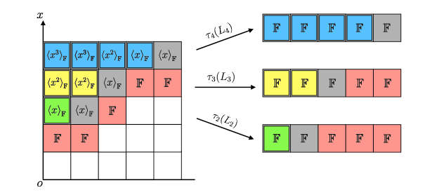
Figure 12: $\mathbb{F}$-relation families and $\mathbb{F}$-framed relation families in dimension $n=1$ (illustration of 4.23).

where

$$\tau_{2}(L_{2}) =\left\langle\tau_{2}(x,0,0,0,0)\right\rangle_{\mathbb{F}}$$

$$=\left\langle(1,0,0,0,0)\right\rangle_{\mathbb{F}}\subseteq\mathbb{F}^{5},$$

$$\tau_{3}(L_{3}) =\left\langle\tau_{3}(x^{2},0,0,0,0),\tau_{3}(0,x^{2},0,0,0)\right\rangle_{\mathbb{F}}$$

$$=\left\langle(1,0,0,0,0),(0,1,0,0,0)\right\rangle_{\mathbb{F}}\subseteq\mathbb{F}^{5},$$

$$\tau_{4}(L_{4}) =\left\langle\tau_{4}(x^{3},0,0,0,0),\tau_{4}(0,x^{3},0,0,0),\tau_{4}(0,0,x^{2},0,0),\tau_{4}(0,0,0,x,0)\right\rangle_{\mathbb{F}}$$

$$=\left\langle(1,0,0,0,0),(0,1,0,0,0),(0,0,1,0,0),(0,0,0,1,0)\right\rangle_{\mathbb{F}}\subseteq\mathbb{F}^{5}$$

Figure 12 illustrates $\theta_{1}^{\mathbb{F}}(\xi_{0},\xi_{1})((L_{j})_{j\in\{2,3,4\}})$. On the left: the blue blocks correspond to $L_{4}$, the yellow blocks correspond to $L_{3}$ and the green block corresponds to $L_{2}$. The red blocks are the "forbidden" blocks that we get from condition $4$ in $R_{1}^{\mathbb{F}}(\xi_{0},\xi_{1})$. On the right: the blue blocks correspond to the image of $L_{4}$ under $\tau_{4}$, the yellow blocks correspond to the image of $L_{3}$ under $\tau_{3}$ and the green block corresponds to the image of $L_{2}$ under $\tau_{2}$. The red books are the "forbidden" blocks that we get from condition $1$ in $Y_{1}^{\mathbb{F}}(\xi_{0},\xi_{1})$.

Example 4.24.

This example can be found in [CZ07, Sec. 5.2], [CZ09, Sec. 5.2] and will be also discussed later in Section 4.4. Let $n=2$. As in 4.4, consider

$$\xi_{0} :=\{{\color[rgb]{0,0,0}((0,0),1),((0,0),2)}\},$$

$$\xi_{1} :=\{((3,0),1),((2,1),1),((1,2),1),((0,3),1)\}.$$

Figure 13 illustrates

$$\theta_{2}^{\mathbb{F}}(\xi_{0},\xi_{1})(L_{(3,0)},L_{(2,1)},L_{(1,2)},L_{(3,0)})$$

$$=(\tau_{(3,0)}(L_{(3,0)}),\tau_{(2,1)}(L_{(2,1)}),\tau_{(1,2)}(L_{(1,2)}),\tau_{(3,0)}(L_{(3,0)}))$$

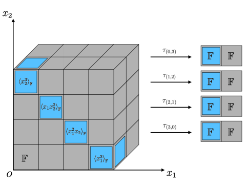
Figure 13: $\mathbb{F}$-relation families and $\mathbb{F}$-framed relation families in dimension $n=2$ (illustration of 4.24).

where

$$L_{(3,0)}:=\braket{(x_{1}^{3},0)}_{\mathbb{F}}\subseteq\mathcal{F}_{2}^{\mathbb{F}}(\xi_{0})_{(3,0)},$$

$$L_{(2,1)}:=\braket{(x_{1}^{2}x_{2},0)}_{\mathbb{F}}\subseteq\mathcal{F}_{2}^{\mathbb{F}}(\xi_{0})_{(2,1)},$$

$$L_{(1,2)}:=\braket{(x_{1}x_{2}^{2},0)}_{\mathbb{F}}\subseteq\mathcal{F}_{2}^{\mathbb{F}}(\xi_{0})_{(1,2)},$$

$$L_{(0,3)}:=\braket{(x_{2}^{3},0)}_{\mathbb{F}}\subseteq\mathcal{F}_{2}^{\mathbb{F}}(\xi_{0})_{(0,3)}.$$

We have

$$\tau_{(3,0)}(L_{(3,0)})=\braket{\tau_{(3,0)}(x_{1}^{3},0)}_{\mathbb{F}}=\braket{(1,0)}_{\mathbb{F}}\subseteq\mathbb{F}^{2},$$

$$\tau_{(2,1)}(L_{(2,1)})=\braket{\tau_{(2,1)}(x_{1}^{2}x_{2},0)}_{\mathbb{F}}=\braket{(1,0)}_{\mathbb{F}}\subseteq\mathbb{F}^{2},$$

$$\tau_{(1,2)}(L_{(1,2)})=\braket{\tau_{(1,2)}(x_{1}x_{2}^{2},0)}_{\mathbb{F}}=\braket{(1,0)}_{\mathbb{F}}\subseteq\mathbb{F}^{2},$$

$$\tau_{(0,3)}(L_{(0,3)})=\braket{\tau_{(0,3)}(x_{2}^{3},0)}_{\mathbb{F}}=\braket{(1,0)}_{\mathbb{F}}\subseteq\mathbb{F}^{2}.$$

Conditions 1-3 in $Y_{2}^{\mathbb{F}}(\xi_{0},\xi_{1})$ are trivial and we obtain

$$Y_{2}^{\mathbb{F}}(\xi_{0},\xi_{1})=\mathrm{G}_{\mathbb{F}}(1,2)^{4}=\mathbb{P}_{1}(\mathbb{F})^{4}$$

where $\mathbb{P}_{1}(\mathbb{F})$ denotes the projective line over $\mathbb{F}$ (the set of all one-dimensional subspaces of $\mathbb{F}^{2}$). Since $\mathrm{GL}_{\preceq}^{\mathbb{F}}(\xi_{0})=\mathrm{GL}_{2}(\mathbb{F})$ (see 4.16), we have

$$I_{2}^{\mathbb{F}}(\xi_{0},\xi_{1})\cong Y_{2}^{\mathbb{F}}(\xi_{0},\xi_{1})/\mathrm{GL}_{\preceq}^{\mathbb{F}}(\xi_{0})=\mathbb{P}_{1}(\mathbb{F})^{4}/\mathrm{GL}_{2}(\mathbb{F})$$

as sets.

Proof of 4.22.

Since $\tau_{w}$ is injective for all $w\in V_{1}$ by construction, $\theta_{n}^{\mathbb{F}}(\xi_{0},\xi_{1})$ is well-defined and injective. So, let us show that $\mathrm{im}(\theta_{n}^{\mathbb{F}}(\xi_{0},\xi_{1}))=Y_{n}^{\mathbb{F}}(\xi_{0},\xi_{1})$.

$\mathrm{im}(\theta_{n}^{\mathbb{F}}(\xi_{0},\xi_{1}))\subseteq Y_{n}^{\mathbb{F}}(\xi_{0},\xi_{1})$: for this, let $(L_{w})_{w\in V_{1}}\in R_{n}^{\mathbb{F}}(\xi_{0},\xi_{1})$. We have to show that $(\tau_{w}(L_{w}))_{w\in V_{1}}$ satisfies conditions 1-3 in $Y_{n}^{\mathbb{F}}(\xi_{0},\xi_{1})$. Let $w\in V_{1}$.

1. By construction of the $\tau_{w}$, it is clear that $\pi_{v}(\tau_{w}(L_{w}))=0$ for all $v\in V_{0}$ with $v\nprec w$.

2. By construction of the $\tau_{v}$, we have $\tau_{v}(L_{v})=\tau_{w}(x^{w-v}L_{v})$ for all $v\in V_{1}$ with $v\prec w$. Hence,

   $$\tau_{v}(L_{v})=\tau_{w}(x^{w-v}L_{v})\subseteq\tau_{w}(L_{w})$$

   for all $v\in V_{1}$ with $v\prec w$.

3. We have $\tau_{w}(L_{w})\cong L_{w}$ as $\mathbb{F}$-vector spaces for all $w\in V_{1}$ and therefore,

   $${\sum_{v\prec w}\tau_{v}(L_{v})\cong\sum_{v\prec w}L_{v}}$$

   as $\mathbb{F}$-vector spaces. We have $\sum_{v\prec w}\tau_{v}(L_{v})\subseteq\tau_{w}(L_{w})$ by condition 2. Thus, we conclude that

   $$\mu_{1}(w)=\mathrm{dim}_{\mathbb{F}}\left(L_{w}/\sum_{v\prec w}L_{v}\right)=\mathrm{dim}_{\mathbb{F}}\left(\tau_{w}(L_{w})/\sum_{v\prec w}\tau_{v}(L_{v})\right).$$

$Y_{n}^{\mathbb{F}}(\xi_{0},\xi_{1})\subseteq\mathrm{im}(\theta_{n}^{\mathbb{F}}(\xi_{0},\xi_{1}))$: let $(L_{w})_{w\in V_{1}}\in Y_{n}^{\mathbb{F}}(\xi_{0},\xi_{1})$. Let $w\in V_{1}$ and $z\in L_{w}$. Then

$$z=(z_{1,1},\dots,z_{1,\mu_{0}(v_{1})},\dots,z_{s_{0},1},\dots,z_{s_{0},\mu_{0}(v_{s_{0}})})$$

for suitable $z_{i,j}\in\mathbb{F}$ where for all $i\in\{1,\dots,s_{0}\}$,

$$v_{i}\nprec w\Longrightarrow\forall\,j\in\{1,\dots,\mu_{0}(v_{i})\}:z_{i,j}=0.$$

Let $i\in\{1,\dots,s_{0}\}$. If $v_{i}\prec w$, define $\widetilde{z}_{i,j}:=x^{w-v_{j}}z_{i,j}$ for all $j\in\{1,\dots,\mu_{0}(v_{i})\}$ and if $v_{i}\nprec w$, define $\widetilde{z}_{i,j}:=0$ for all $j\in\{1,\dots,\mu_{0}(v_{i})\}$. Let

$$\widetilde{z}:=(\widetilde{z}_{1,1},\dots,\widetilde{z}_{1,\mu_{0}(v_{1})},\dots,\widetilde{z}_{s_{0},1},\dots,\widetilde{z}_{s_{0},\mu_{0}(v_{s_{0}})})$$

and define $\widetilde{L}_{w}:=\{\widetilde{z}\mid z\in L_{w}\}$. Then $(\widetilde{L}_{w})_{w\in V_{1}}\in R_{n}^{\mathbb{F}}(\xi_{0},\xi_{1})$ and

$$\theta_{n}^{\mathbb{F}}(\xi_{0},\xi_{1})((\widetilde{L}_{w})_{w\in V_{1}})=(L_{w})_{w\in V_{1}}.$$

Thus, we conclude that $Y_{n}^{\mathbb{F}}(\xi_{0},\xi_{1})\subseteq\mathrm{im}(\theta_{n}^{\mathbb{F}}(\xi_{0},\xi_{1}))$. The rest is clear by construction of $\psi_{n}^{\mathbb{F}}(\xi_{0})$. ∎

4.4 The non-existence of a discrete and complete invariant

Using the parameterization result of the last section, we are now able to give a universal counterexample for any $n\geq 2$, which proves the non-existence of a discrete class of complete invariants

$$\left\{f_{n}^{\mathbb{F}}:\mathbf{Grf}_{n}(A_{n}^{\mathbb{F}})/_{\cong}\longrightarrow Q_{n}^{\mathbb{F}}\right\}_{\mathbb{F}\in\mathcal{K}}.$$

The following counter example can be found in [CZ07, Sec. 5.2] and[CZ09, Sec. 5.3] (see also 4.24). We just generalize it in a very natural way from $n=2$ to $n\geq 2$. For $n=2$, define

$$v_{2,1}:=(3,0),\quad v_{2,2}:=(2,1),\quad v_{2,3}:=(1,2),\quad v_{2,4}:=(0,3)$$

and for $n\geq 3$, define

$$v_{n,1} :=(3,0,0,\dots,0),\quad v_{n,2}:=(2,1,0,\dots,0),$$

$$v_{n,3} :=(1,2,0,\dots,0),\quad v_{n,4}:=(0,3,0,\dots,0).$$

Now let

$$\xi_{n,0} :=\{((0,\dots,0),1),((0,\dots,0),2)\},$$

$$\xi_{n,1} :=\{(v_{n,1},1),(v_{n,2},1),(v_{n,3},1),(v_{n,4},1)\}.$$

Proposition 4.25.

If $\mathbb{F}$ is finite we have

$$\infty>\left\lvert I_{n}^{\mathbb{F}}(\xi_{n,0},\xi_{n,1})\right\lvert\geq\left\lvert\mathbb{F}\right\lvert-2.$$

If $\mathbb{F}$ is countable $I_{n}^{\mathbb{F}}(\xi_{n,0},\xi_{n,1})$ is countable and if $\mathbb{F}$ is uncountable $I_{n}^{\mathbb{F}}(\xi_{n,0},\xi_{n,1})$ is uncountable.

Proof.

We have $m_{0}=2$, $\mathrm{GL}_{\preceq}^{\mathbb{F}}(\xi_{n,0})=\mathrm{GL}_{2}(\mathbb{F})$ (see 4.16) and $\delta_{1}(v_{n,i})=1$ for all $i\in\{1,\dots,4\}$. Conditions $1$-$3$ in 4.20 are all trivial. Therefore,

$$Y_{n}^{\mathbb{F}}(\xi_{0},\xi_{1})=\mathrm{G}_{\mathbb{F}}(1,2)^{4}=\mathbb{P}_{1}(\mathbb{F})^{4}$$

where $\mathbb{P}_{1}(\mathbb{F})$ denotes the projective line over $\mathbb{F}$ (the set of all one-dimensional subspaces of $\mathbb{F}^{2}$). By 4.22, we obtain a set theoretic bijection

$$I_{n}^{\mathbb{F}}(\xi_{n,0},\xi_{n,1})\cong{\mathbb{P}_{1}(\mathbb{F})^{4}}/{\mathrm{GL}_{2}(\mathbb{F})}.$$

Now let

$$\Omega:=\{(l_{1},l_{2},l_{2},l_{4})\in\mathbb{P}_{1}(\mathbb{F})^{4}\mid l_{i}\neq l_{j}\,\mathrm{for}\,i\neq j\}\subseteq\mathbb{P}_{1}(\mathbb{F})^{4}$$

be the subspace of pairwise distinct lines. $\Omega$ is clearly $\mathrm{GL}_{2}(\mathbb{F})$ invariant and we have ${\mathbb{P}_{1}(\mathbb{F})^{4}}/{\mathrm{GL}_{2}(\mathbb{F})}\supseteq{\Omega}/{\mathrm{GL}_{2}(\mathbb{F})}$.

We show that $\Omega/\mathrm{GL}_{2}(\mathbb{F})\cong\mathbb{F}\setminus\{0,1\}$ as sets: let

$$((a_{1}:a_{2}),(b_{1}:b_{2}),(c_{1}:c_{2}),(d_{1}:d_{2}))\in\Omega.$$

As $(a_{1}:a_{2})\neq(b_{1}:b_{2})$, we have $\mathbb{F}^{2}=\braket{(a_{1},a_{2}),(b_{1},b_{2})}_{\mathbb{F}}$ which shows that

$$M:=\begin{pmatrix}a_{1}&b_{1}\\ a_{2}&b_{2}\end{pmatrix}\in\mathrm{GL}_{2}(\mathbb{F}).$$

Hence,

$$(M^{-1}(a_{1}:a_{2}),M^{-1}(b_{1}:b_{2}),M^{-1}(c_{1}:c_{2}),M^{-1}(d_{1}:d_{2}))$$

$$= ((1:0),(0:1),M^{-1}(c_{1}:c_{2}),M^{-1}(d_{1}:d_{2})).$$

Now let $(\widetilde{c_{1}}:\widetilde{c_{2}}):=M^{-1}(c_{1}:c_{2})$. As $(\widetilde{c_{1}}:\widetilde{c_{2}})\neq(1:0),(0:1)$,

$$D:=\begin{pmatrix}\frac{1}{c_{1}}&0\\ 0&\frac{1}{c_{2}}\end{pmatrix}\in\mathrm{GL}_{2}(\mathbb{F})$$

is well-defined and we obtain

$$(D(1:0),D(0:1),D(\widetilde{c_{1}}:\widetilde{c_{2}}),DM^{-1}(d_{1}:d_{2}))$$

$$= ((1:0),(0:1),(1:1),DM^{-1}(d_{1}:d_{2})).$$

Thus, we have

$$\Omega/\mathrm{GL}_{2}(\mathbb{F})=\{ \mathrm{GL}_{2}(\mathbb{F})\cdot(l_{1},l_{2},l_{3},l_{4})\mid$$

$$l_{1}=(1:0),l_{2}=(0:1),l_{3}=(1:1),l_{4}=(x:y)\neq l_{1},l_{2},l_{3}\}$$

which shows that the assignment

$$\Omega/\mathrm{GL}_{2}(\mathbb{F})\xlongrightarrow{\sim}\mathbb{P}_{1}(\mathbb{F})\setminus\{(1:0),(0:1),(1:1)\},\quad\mathrm{GL}_{2}(\mathbb{F})\cdot(l_{1},l_{2},l_{3},l_{4})\longmapsto l_{4}$$

is a bijection of sets. Since

$${\mathbb{P}_{1}(\mathbb{F})^{4}}/{\mathrm{GL}_{2}(\mathbb{F})}\supseteq{\Omega}/{\mathrm{GL}_{2}(\mathbb{F})}\cong\mathbb{P}_{1}(\mathbb{F})\setminus\{(1:0),(0:1),(1:1)\}\cong\mathbb{F}\setminus\{0,1\}$$

as sets, the statement follows. ∎

This shows that for $n\geq 2$, there exists no discrete class of complete invariants

$$\{f_{\mathbb{F}}:\mathbf{Grf}_{n}(A_{n}^{\mathbb{F}})/_{\cong}\longrightarrow Q_{n}^{\mathbb{F}}\}_{\mathbb{F}\in\mathcal{K}}.$$

4.5 The moduli space

Let us start with recalling some standard material: Let $\mathcal{D}$ be a category,

$$F:\mathcal{D}^{\mathrm{opp}}\longrightarrow\mathrm{Sets}$$

a functor and $(S,\beta)$ a pair with $S\in\mathcal{D}$ and $\beta\in F(S)$. If the assignment

$$\mathrm{Hom}_{\mathcal{D}}(T,S)\longrightarrow F(T),\quad f\longmapsto F(f)(\beta)$$

is a bijection for all $T\in\mathcal{D}$, then $F$ is called representable by $(S,\beta)$. Note that if there exists an isomorphism $g:\mathrm{Hom}_{\mathcal{D}}(-,S)\to F$, then $F$ is representable by $(S,g(\mathrm{id}_{S}))$ and we just say that $F$ is representable by $S$ if there exists such an isomorphism. Let $S$ be a scheme. An $S$-scheme $X$ is a scheme $X$ together with a morphism of schemes $X\to S$. A morphism of $S$-schemes $X\to Y$ is a morphism of schemes such that the diagram

commutes. Denote by

1. $\mathrm{LNSch}_{\mathbb{F}}$ the category of locally Noetherian $\mathbb{F}$-schemes,

2. $\mathrm{NAff}_{\mathbb{F}}$ the category of Noetherian affine $\mathbb{F}$-schemes and

3. $\mathrm{NAlg}_{\mathbb{F}}$ the category of Noetherian $\mathbb{F}$-algebras.

Any $X\in\mathrm{LNSch}_{\mathbb{F}}$ defines a functor (the so-called functor of points)

$$h_{X}:\mathrm{LNSch}_{\mathbb{F}}^{\mathrm{opp}}\longrightarrow\mathrm{Sets},\quad Y\longmapsto\mathrm{Hom}_{\mathbb{F}}(Y,X)$$

We often use the notation $h_{X}(-):=X(-)$. By Yoneda‘s Lemma, the scheme $X$ is completely determined by its functor of points $h_{X}$. Moreover, $h_{X}$ is completey determined by its restriction to $\mathrm{NAff}_{\mathbb{F}}^{\mathrm{opp}}$ (or $\mathrm{NAlg}_{\mathbb{F}}$ since $\mathrm{NAff}_{\mathbb{F}}^{\mathrm{opp}}$ is equivalent to $\mathrm{NAlg}_{\mathbb{F}}$) (see [EH00, Prop. VI-2, Ex. VI-3]).

Definition 4.26.

Let $S$ be a scheme and $X,Y$ be $S$-schemes. $Y$ is called an open/closed subscheme of $X$ if there exists a morphism of $S$-schemes $Y\to X$ which is an open/closed immersion. In this case, we often simply say that $Y\subseteq X$ is an open/closed subscheme.

The following definition is standard material about schemes. See for example [GW10, Def. 3.9] where it is formulated for $\mathrm{Spec}({\mathbb{Z}})$-schemes (for $S$-schemes everything is analogous).

Definition 4.27 (Gluing Datum).

Let $S$ be a scheme. A gluing datum of $S$-schemes consists of the following data:

1. an index set $I$,

2. for all $i\in I$, an $S$-scheme $U_{i}$,

3. for all $i,j\in I$ an open subset $U_{i,j}\subseteq U_{i}$ (we consider $U_{ij}$ as open subschemes of $U_{i}$),

4. for all $i,j\in I$ an isomorphism $\varphi_{ji}:U_{ij}\to U_{ji}$ of $S$-schemes,

such that

1. $U_{ii}=U_{i}$ for all $i\in I$

2. the cocycle condition holds: $\varphi_{kj}\circ\varphi_{ji}=\varphi_{ki}$ on $U_{ij}\cap U_{ik}$ for all $i,j,k\in I$.

Note that we implicitly assume in the cocycle condition that $\varphi_{ji}(U_{ij}\cap U_{ik})\subseteq U_{jk}$ (such that the composition is meaningful). For $i=j=k$, the cocycle condition implies that $\varphi_{ii}=\mathrm{id}_{U_{i}}$ and (for $i=k$), $\varphi_{ji}:U_{ij}\xrightarrow{\sim}U_{ji}$ is an isomorphism of $S$-schemes with $\varphi_{ij}^{-1}=\varphi_{ji}$.

The following proposition is standard material about schemes. See for example [GW10, Prop. 3.10] where it is formulated for $\mathrm{Spec}({\mathbb{Z}})$-schemes (for $S$-schemes everything is analogous).

Proposition 4.28 (Gluing Schemes).

Let $S$ be a scheme and

$$((U_{i})_{i\in I},(U_{ij})_{i,j\in I},(\varphi_{ij})_{i,j\in I})$$

a gluing datum of $S$-schemes. Then there exists an $S$-scheme $X$ together with $S$-morphisms $\psi_{i}:U_{i}\to X$ for all $i\in I$ such that

1. for all $i\in I$, the map $\psi_{i}$ yields an $S$-isomorphism from $U_{i}$ onto an open subscheme of $X$,

2. $\psi_{j}\circ\varphi_{ji}=\psi_{i}$ for all $i,j\in I$,

3. $X=\bigcup_{i\in I}\psi_{i}(U_{i})$,

4. $\psi_{i}(U_{i})\cap\psi_{j}(U_{j})=\psi_{i}(U_{ij})=\psi_{j}(U_{ji})$ for all $i,j\in I$.

Furthermore, $X$ together with the $\psi_{i}$ is uniquely determined up to unique $S$-isomorphism. We usually identify $U_{i}=\psi_{i}(U_{i})\subseteq X$ and write $X=\bigcup_{i\in I}U_{i}$ as well as

$$U_{i}\cap U_{j}=\psi_{i}(U_{i})\cap\psi_{j}(U_{j})=\psi_{i}(U_{ij})=\psi_{j}(U_{ij})=U_{ij}.$$

Definition 4.29.

Let $m\in\mathbb{N}$. Denote by

1. $\mathbb{A}_{\mathbb{F}}^{m}=\mathrm{Spec}(\mathbb{F}[x_{1},\dots,x_{m}])$ the affine space of dimension $m$ as $\mathbb{F}$-scheme,

2. $\mathbb{P}_{\mathbb{F}}^{m}=\mathrm{Proj}(\mathbb{F}[x_{0},\dots,x_{m}])$ the projective space of dimension $m$ as $\mathbb{F}$-scheme and

3. $\mathbb{P}_{m}(\mathbb{F})$ the projective space of dimension $m$ as the set of all one-dimensional subspaces of $\mathbb{F}^{m+1}$.

Note that we have $\mathbb{A}_{\mathbb{F}}^{m}(\mathbb{F})=\mathbb{F}^{m}$ and $\mathbb{P}_{\mathbb{F}}^{m}(\mathbb{F})=\mathbb{P}_{m}(\mathbb{F})$.

Definition 4.30 (Projective $\mathbb{F}$-scheme).

An $\mathbb{F}$-scheme $X$ is called a projective $\mathbb{F}$-scheme if there exists a natural number $m\in\mathbb{N}$ such that $X\subseteq\mathbb{P}^{m}_{\mathbb{F}}$ is a closed subscheme.

Definition 4.31.

Let $X$ be an $\mathbb{F}$-scheme.

1. $X$ is called an affine $\mathbb{F}$-variety if $X=\mathrm{Spec}(R)$ for a finitely generated $\mathbb{F}$-alegbra $R$.

2. $X$ is called an $\mathbb{F}$-variety if $X=\bigcup_{i=1}^{m}X_{i}$ where $X_{i}\subseteq X$ is open and an affine variety for all $i\in\{1,\dots,m\}$.

3. $X$ is called a projective $\mathbb{F}$-variety if $X$ is an $\mathbb{F}$-variety and a projective $\mathbb{F}$-scheme.

4. Let $X,Y$ be $\mathbb{F}$-varieties. $Y$ is called an open/closed subvariety of $X$ if $Y$ is an open/closed subscheme of $X$.

5. Let $X,Y$ be $\mathbb{F}$-varieties. Then $Y$ is called a subprevariety of $X$ if there exists a closed subvariety $Z\subseteq X$ such that $Y\subseteq Z$ is an open subvariety.

4.5.1 Parameterization as a subprevariety

We begin this section with the realization of $\mathrm{G}_{\mathbb{F}}(d,m)$ as the set of $\mathbb{F}$-points of a projective $\mathbb{F}$-scheme $\mathcal{G}_{\mathbb{F}}(d,m)$, the so-called Grassmann scheme. There are different ways to construct $\mathcal{G}_{\mathbb{F}}(d,m)$. Our construction follows that in [EH00, III.2.7] and focuses on the technical details that are missing in [EH00].

Theorem 4.32.

Let $d,m\in\mathbb{N}$ with $d\leq m$. Then there exists a projective $\mathbb{F}$-scheme $\mathcal{G}_{\mathbb{F}}(d,m)$ (the Grassmann scheme) together with a set theoretic bijection

$$\mathcal{G}_{\mathbb{F}}(d,m)(\mathbb{F})\xlongrightarrow{\sim}\mathrm{G}_{\mathbb{F}}(d,m).$$

If $d>m$, we set $\mathcal{G}_{\mathbb{F}}(d,m):=\emptyset$.

Proof.

Let $L\in\mathrm{G}_{\mathbb{F}}(d,m)$. Pick an $\mathbb{F}$-basis $B_{L}$ of $L$ and define $M(B_{L})\in M_{d\times m}(\mathbb{F})$ as the matrix which has the transposed basis vectors as entries. Let

$$M_{d\times m}(\mathbb{F})_{d}:=\{M\in M_{d\times m}(\mathbb{F})\mid\mathrm{rank}(M)=d\}.$$

For $M,N\in M_{d\times m}(\mathbb{F})_{d}$, define $M\sim N$ if and only if $A\cdot M=N$ for some $A\in\mathrm{GL}_{d}(\mathbb{F})$. Then

$$\eta:\mathrm{G}_{\mathbb{F}}(d,m)\longrightarrow M_{d\times m}(\mathbb{F})_{d}/_{\sim},\quad L\longmapsto[M(B_{L})]$$

is a well-defined bijection. Define $\mathcal{I}:=\{(i_{1}<\dots<i_{d})\mid 1\leq i_{j}\leq m\}$. Let

$$[M]\in M_{d\times m}(\mathbb{F})_{d}/_{\sim}.$$

Since $\mathrm{rk}(M)=d$ there exists an $I\in\mathcal{I}$ such that $\mathrm{det}(M_{I})\neq 0$. Hence, $(M_{I}^{-1}M)_{I}=1_{d}$. Here $M_{I}$ denotes the $I$-th submatrix of $M$. $\mathrm{det}(M_{I})$ is also called the $I$-th minor of $M$. For $I\in\mathcal{I}$, let

$$U(I) :=\{[M]\in M_{d\times m}(\mathbb{F})/_{\sim}\mid\mathrm{det}(M_{I})\neq 0\},$$

$$V(I) :=\{L\in\mathrm{G}_{\mathbb{F}}(d,m)\mid L\oplus\braket{\{e_{i}\}_{i\in I^{c}}}=\mathbb{F}^{m}\},$$

$$W(I) :=\{M\in M_{d\times m}(\mathbb{F})\mid M_{I}={1}_{d}\}.$$

Then $\bigcup_{I\in\mathcal{I}}V(I)=\mathrm{G}_{\mathbb{F}}(d,m)$, $\bigcup_{I\in\mathcal{I}}U(I)=M_{d\times m}(\mathbb{F})/_{\sim}$ and $\eta|_{V(I)}=U(I)$. We obtain a well-defined bijection

$$\lambda(I):U(I)\longrightarrow W(I),\quad[M]\longmapsto M_{I}^{-1}M$$

Note that $W(I)\cong\mathbb{A}^{m(m-d)}_{\mathbb{F}}(\mathbb{F})$ as sets. For $I,J\in\mathcal{I}$, define

$$W(I,J):=\{M\in W(I)\mid\mathrm{det}(M_{J})\neq 0\}$$

Then we have $W(I,I)=W(I)$ and set theoretic bijections

$$\varphi_{IJ}:W(I,J)\longrightarrow W(J,I),\quad M\longmapsto M_{J}^{-1}M.$$

Now let $X:=\bigcup_{I\in\mathcal{I}}W(I)/_{\sim}$ where for $x\in W(I)$ and $y\in W(J)$, $x\sim y$ if $x\in W(I,J)$, $y\in W(J,I)$ and $\varphi_{IJ}(x)=y$. We obtain a well-defined set theoretic bijection

$$\lambda:\bigcup_{I\in\mathcal{I}}U(I)\longrightarrow X,\quad U(I)\ni x\longmapsto\lambda(I)(x)$$

and hence a set theoretic bijection

$$\lambda\circ\eta:\mathrm{G}_{\mathbb{F}}(d,m)\longrightarrow X.$$

The next step is to translate everything into polynomial equations. Let ${R:=\mathbb{F}[(x_{ij})]}$ be the polynomial ring in $dm$ variables. Then $\mathcal{W}:=\mathrm{Spec}(R)\cong\mathbb{A}_{\mathbb{F}}^{dm}$. Let ${K(I):=\braket{(x_{i,j})_{I}-1_{d}}}$ and $R(I):=R/K(I)$. Now

$$\mathcal{W}(I):=\mathrm{Spec}(R(I))$$

is a closed subscheme of $\mathcal{W}$ with $\mathcal{W}(I)(\mathbb{F})=W(I)$. For $J\in\mathcal{I}$, define

$$R(I,J):=R(I)\left[\mathrm{det}((x_{ij})_{J})^{-1}\right]$$

and

$$\mathcal{W}(I,J):=\mathrm{Spec}(R(I,J)).$$

$\mathcal{W}(I,J)$ is an open subscheme of $\mathcal{W}(I)$. We have $\mathcal{W}(I,I)=\mathcal{W}(I)$ and for any $T\in\mathrm{NAlg}_{\mathbb{F}}$, we obtain

$$\mathcal{W}(I)(T)=\mathrm{Hom}_{\mathbb{F}}(R(I),T)=\{M\in M_{d\times m}(T)\mid M_{I}=1_{d}\}$$

and

$$\mathcal{W}(I,J)(T)=\mathrm{Hom}_{\mathbb{F}}(R(I,J),T)=\{M\in\mathcal{W}(I)(S)\mid\mathrm{det}(M_{J})\in T^{\times}\}.$$

The assignment

$$\varphi_{JI}(T):\mathcal{W}(I,J)(T)\longrightarrow\mathcal{W}(J,I)(T),\quad M\longmapsto M_{J}^{-1}M.$$

is a set theoretic bijection and natural in $T$. Hence, we obtain an isomorphism of $\mathbb{F}$-schemes

$$\varphi_{JI}:\mathcal{W}(I,J)\longrightarrow\mathcal{W}(J,I).$$

We have for all $M\in\mathcal{W}(I,J)(T)\cap\mathcal{W}(I,K)(T)$,

$$(\varphi_{KJ}(T)\circ\varphi_{JI}(T))(M) =\varphi_{KJ}(T)(M_{I}^{-1}M)=M_{K}^{-1}M_{I}^{-1}M$$

$$\overset{M_{I}=1_{d}}{=}M_{K}^{-1}M=\varphi_{KI}(T)(M)$$

which shows that the cocycle condition is satisfied. Now use 4.28 to define $\mathcal{G}_{\mathbb{F}}(d,m)$ as the $\mathbb{F}$-scheme that one obtains by gluing the $\mathcal{W}(I)$ along the $\varphi_{JI}$. By Construction, we have $\mathcal{G}_{\mathbb{F}}(d,m)(\mathbb{F})=X$ and $(\eta\circ\lambda)^{-1}$ is a set theoretic bijection from $\mathcal{G}_{\mathbb{F}}(d,m)(\mathbb{F})$ to $\mathrm{G}_{\mathbb{F}}(d,m)$. So, from an intuitive point of view, this construction is the correct one if we consider $\mathbb{F}$-points. That $\mathcal{G}_{\mathbb{F}}(d,m)$ is a projective variety follows from [EH00, Ex. III-49] or [GW10, (8.10)]. ∎

The next theorem is based on and inspired by [CZ09, Sec. 5] and [CZ07, Thm. 4]. In order to realize $Y_{n}^{\mathbb{F}}(\xi_{0},\xi_{1})$ as a subprevariety of a product of Grassmann varieties, we have to translate conditions 1-3 in the definition of $Y_{n}^{\mathbb{F}}(\xi_{0},\xi_{1})$ (see 4.20) into polynomial equations. This translation is spelled out in [CZ09, Sec. 5] (without the first condition in the definition of $Y_{n}^{\mathbb{F}}(\xi_{0},\xi_{1})$) while in [CZ07] the authors only state the theorem (here the first and third condition in $Y_{n}^{\mathbb{F}}(\xi_{0},\xi_{1})$ are missing). Our proof follows [CZ09, Sec. 5] with a focus on the technical details and on the translation of the first condition in the definition of $Y_{n}^{\mathbb{F}}(\xi_{0},\xi_{1})$ into polynomial equations.

Theorem 4.33.

There exists a subprevariety

$$\mathcal{Y}_{n}^{\mathbb{F}}(\xi_{0},\xi_{1})\subseteq\prod_{w\in V_{1}}\mathcal{G}_{\mathbb{F}}(\delta_{1}(w),m_{0})$$

and a set theoretic bijection

$$\mathcal{Y}_{n}^{\mathbb{F}}(\xi_{0},\xi_{1})(\mathbb{F})\xlongrightarrow{\sim}Y_{n}^{\mathbb{F}}(\xi_{0},\xi_{1}).$$

Proof.

Before we start with the proof, we introduce some notations:

1. recall that $\xi_{0}=(V_{0},\mu_{0})$, $\xi_{1}=(V_{1},\mu_{1})$, ${\delta_{1}(w)=\mathrm{dim}_{\mathbb{F}}(\mathcal{F}_{n}^{\mathbb{F}}(\xi_{1})_{w})}$ for all $w\in\mathbb{N}^{n}$, ${m_{0}=\left\lvert\xi_{0}\right\lvert=\sum_{v\in V_{0}}\mu_{0}(v)}$ and that we indentify $\mathbb{F}^{m_{0}}=\bigoplus_{v\in V_{0}}\mathbb{F}^{\mu_{0}(v)}$ along our enumeration of ${V_{0}=\{v_{1},\dots,v_{s_{0}}\}}$. For $w\in V_{1}$, let

   $$I_{w}=\left(i^{(w)}_{1}<\dots<i^{(w)}_{\delta_{1}(w)}\right)$$

   with $1\leq i^{(w)}_{t}\leq m_{0}$. Denote by $\mathcal{I}(w)$ the set of all such sets $I_{w}$ and define

   $${\mathcal{J}:=\prod_{w\in V_{1}}\mathcal{I}(w)}.$$

   We have an open covering of $\prod_{w\in V_{1}}\mathcal{G}_{\mathbb{F}}(\delta_{1}(w),m_{0})$ by affines that are isomorphic to $\mathcal{W}(I)$ where $\mathcal{W}(I):=\prod_{w\in V_{1}}\mathcal{W}(I_{w})$ with ${I=(I_{w})_{w\in V_{1}}\in\mathcal{J}}$ (see proof of 4.32). We have

   $$\mathcal{W}(I)(\mathbb{F})=\prod_{w\in V_{1}}\mathcal{W}(I_{w})(\mathbb{F})=\prod_{w\in V_{1}}W(I_{w}).$$

   Define $W(I):=\prod_{w\in V_{1}}W(I_{w})$.

2. for $w\in V_{1}$, let $\underline{x}(w):=\left(x^{(w)}_{ij}\right)$ where $1\leq i\leq\delta_{1}(w)$, $1\leq j\leq m_{0}$. By adapting the notations of the proof of 4.32, define

   $$R:=\mathbb{F}\left[(\underline{x}({w}))_{w\in V_{1}}\right],\quad K\left(I\right):=\left\langle\bigcup_{w\in V_{1}}K\left(I_{w}\right)\right\rangle,\quad R(I):=R/K(I)$$

   where $I=(I_{w})_{w\in V_{1}}\in\mathcal{J}$. Then $\mathcal{W}\left(I\right)=\mathrm{Spec}(R(I))$. For $J\in\mathcal{J}$, $\mathcal{W}(I,J)$ is defined analogously and we obtain canonical isomorphisms

   $$\varphi_{JI}:\mathcal{W}(I,J)\to\mathcal{W}(J,I)$$

   such that $\prod_{w\in V_{1}}\mathcal{G}_{\mathbb{F}}(\delta_{1}(w),m_{0})$ results by gluing the $\mathcal{W}(I)$ along the $\varphi_{JI}$.

3. for $w\in V_{1}$, let

   $$\eta_{w}:\mathrm{G}_{\mathbb{F}}(\delta_{1}(w),m_{0})\longrightarrow M_{\delta_{1}(w)\times m_{0}}(\mathbb{F})_{\delta_{1}(w)}/_{\sim}$$

   and

   $$\lambda_{I_{w}}:U(I_{w})\longrightarrow W(I_{w})$$

   as before (see proof of 4.32). We have a set theoretic bijection

   $$\gamma_{I_{w}}:=\lambda_{I_{w}}\circ\eta_{w}|_{V(I_{w})}:V(I_{w})\longrightarrow W(I_{w}).$$

To show the existence of a subprevariety

$$\mathcal{Y}_{n}^{\mathbb{F}}(\xi_{0},\xi_{1})\subseteq\prod_{w\in V_{1}}\mathcal{G}_{\mathbb{F}}(\delta_{1}(w),m_{0})\quad\textrm{with}\quad{Y}_{n}^{\mathbb{F}}(\xi_{0},\xi_{1})\cong\mathcal{Y}_{n}^{\mathbb{F}}(\xi_{0},\xi_{1})(\mathbb{F})$$

we have to interprete conditions 1-3 in 4.20 via polynomial equations. Recall that $(L_{w})_{w\in V_{1}}\in\prod_{w\in V_{1}}\mathrm{G}_{\mathbb{F}}(\delta_{1}(w),m_{0})$ is in $Y_{n}^{\mathbb{F}}(\xi_{0},\xi_{1})$ if and only if for all $w\in V_{1}$:

1. $\pi_{v}(L_{w})=0$ for all $v\in V_{0}$ with $v\nprec w$ where $\pi_{v}:\mathbb{F}^{m_{0}}\to\mathbb{F}^{\mu_{0}(v)}$ denotes the canonical projection.

2. if $v\in V_{1}$ with $v\prec w$, then $L_{v}\subseteq L_{w}$.

3. $\mathrm{dim}_{\mathbb{F}}\left(L_{w}/\sum_{v\prec w}L_{v}\right)=\mu_{1}(w)$.

Note that every $(L_{w})_{w\in V_{1}}\in\prod_{w\in V_{1}}\mathrm{G}_{\mathbb{F}}(\delta_{1}(w),m_{0})$ corresponds to a familiy of matrices $(\gamma_{I_{w}}(L_{w}))_{w\in V_{1}}\in W(I)$ for some $I=(I_{w})_{w\in V_{1}}\in\mathcal{J}$.

1. For $w\in V_{1}$, let $Q_{0}(w):=\{v\in V_{0}\mid v\nprec w\}$. Condition $1$ tells us that if $v\in Q_{0}(w)$ we have $\pi_{v}(L_{w})=0$ where $\pi_{v}:\mathbb{F}^{m_{0}}\to\mathbb{F}^{\mu_{0}(v)}$ denotes the canonical projection. In particular, $\mathbb{F}^{\mu_{0}(v)}$ corresponds to a subsummand of

   $$\mathbb{F}^{m_{0}}=\bigoplus_{v\in V_{0}}\mathbb{F}^{\mu_{0}(v)}=\bigoplus_{j=1}^{s_{0}}\mathbb{F}^{\mu_{0}(v_{j})}.$$

   Define

   $$T(v_{j}):=\left\{\left(\sum_{i=1}^{\mu_{0}(v_{j-1})}\mu_{0}(i)\right)+1,\dots,\mu_{0}(v_{j})\right\}$$

   Then

   $$\mathbb{F}^{m_{0}}=\bigoplus_{v\in V_{0}}\mathbb{F}^{\mu_{0}(v)}=\bigoplus_{j=1}^{s_{0}}\mathbb{F}^{\mu_{0}(v_{j})}=\bigoplus_{j=1}^{s_{0}}\bigoplus_{i\in T(v_{j})}\mathbb{F}_{i}$$

   where $\mathbb{F}_{i}=\mathbb{F}$. For $(\gamma_{I_{w}}(L_{w}))_{w\in V_{1}}\in W(I)$, condition $1$ now means that

   $$\forall\,w\in V_{1}\,\forall\,k\in\{1,\dots,s_{0}\}\,\forall\,j\in\{1,\dots,m_{0}\}\,\forall\,i\in\{1,\dots,\delta_{1}(w)\}:$$

   $$v_{k}\in Q_{0}(w),\,j\in T(v_{k})\Longrightarrow(\gamma_{I_{w}}(L_{w}))_{i,j}=0.$$

   Define

   $$P:=\bigcup_{w\in V_{1}}\bigcup_{v_{k}\in Q_{0}(w)}\left\{x^{(w)}_{i,j}\mid j\in T(v_{k}),\,i=1,\dots,\delta_{1}(w)\right\}.$$

   Then

   $$(\gamma_{I_{w}}(L_{w}))_{w\in V_{1}}\in\mathrm{Spec}\left(R/\braket{P,K(I)}\right)(\mathbb{F})\subseteq W(I)$$

   if and only if $(L_{w})_{w\in V_{1}}$ satisfies condition $1.$

2. Now we interprete condition $2$ via polynomial equations. So, let $v,w\in V_{1}$ with $v\prec w$. We wish to find a condition in terms of polynomial equations which captures the property $L_{v}\subseteq L_{w}$. $L_{v}\subseteq L_{w}$ is equivalent to that each row of $\gamma_{I_{v}}(L_{v})$ lies in the $\mathbb{F}$-span of the rows of $\gamma_{I_{w}}(L_{w})$. Since the rank of

   $$A:=\begin{pmatrix}\gamma_{I_{w}}(L_{w})\\ \gamma_{I_{v}}(L_{v})\end{pmatrix}$$

   is at least $\delta_{1}(w)$ this is equivalent to that all $\delta_{1}(w)+1$ minors of $A$ vanish. This minor vanishing condition can interpreted via polynomial equations as follows: let

   $$M(v,w):=\begin{pmatrix}x_{1,1}^{(w)}&\dots&x_{1,m_{0}}^{(w)}\\ \vdots&&\vdots\\ x_{\delta_{1}(w),1}^{(w)}&\dots&x_{\delta_{1}(w),m_{0}}^{(w)}\\ x_{1,1}^{(v)},&\dots&,x_{1,m_{0}}^{(v)}\\ \vdots&&\vdots\\ x_{\delta_{1}(v),1}^{(v)},&\dots&,x_{\delta_{1}(v),m_{0}}^{(v)}\end{pmatrix}$$

   Let $\mathcal{D}(v,w)$ be the set of all $J=(i_{1}<\dots<i_{\delta_{1}(w)+1})$ with $1\leq i_{j}\leq i_{m_{0}}$ such that $M(v,w)_{J}$ is a submatrix of $M(v,w)$. Now define

   $$M :=\{\mathrm{det}(M(v,w)_{J})\mid v,w\in V_{1}:v\prec w,J\in\mathcal{D}(v,w)\},$$

   $$X(I) :=R/\braket{P,M,K(I)},$$

   $$\mathcal{X}(I) :=\mathrm{Spec}(X(I)).$$

   Then $\mathcal{X}(I)$ is a closed subscheme of $\mathcal{W}(I)$ and

   $$(\gamma_{I_{w}}(L_{w}))_{w\in V_{1}}\in\mathcal{X}(I)(\mathbb{F})\subseteq W(I)$$

   if and only if $(L_{w})_{w\in V_{1}}$ satisfies conditions $2$ and $1.$

3. Recall that condition $3$ is that $\mathrm{dim}_{\mathbb{F}}\left(L_{w}/\sum_{v\prec w}L_{v}\right)=\mu_{1}(w)$ for all $w\in V_{1}$. Note that this condition already includes the condition that $L_{v}\subseteq L_{w}$ for all $v\prec w$. Let us assume that $(L_{w})_{w\in V_{1}}$ satisfies condition $2$ and let $w\in V_{1}$. Define ${Q_{1}(w):=\{v\in V_{1}\mid v\prec w\}}$ and enumerate

   $$Q_{1}(w)=\{v(w)_{1},\dots,v(w)_{u}\}$$

   where $u=\left\lvert Q_{1}(w)\right\lvert$. Now $\mathrm{dim}_{\mathbb{F}}\left(L_{w}/\sum_{v\prec w}L_{v}\right)=\mu_{1}(w)$ is equivalent to that

   $$N(w):=\begin{pmatrix}\gamma_{I_{v(w)_{1}}}(L_{v(w)_{1}})\\ \vdots\\ \gamma_{I_{v(w)_{u}}}(L_{v(w)_{u}})\end{pmatrix}$$

   has rank $m_{0}-\mu_{1}(w)$. This is equivalent to that all the $m_{0}-\mu_{1}(w)+1$ minors vanish and that some $m_{0}-\mu_{1}(w)$ minor does not vanish. So, consider the matrix

   $$H(w):=\begin{pmatrix}x_{1,1}^{(v(w)_{1})},&\dots&,x_{1,m_{0}}^{(v(w)_{1})}\\ \vdots&&\vdots\\ x_{\delta_{1}(v(w)_{1}),1}^{(v(w)_{1})},&\dots&,x_{\delta_{1}(v(w)_{1}),m_{0}}^{(v(w)_{1})}\\ \vdots&&\vdots\\ x_{1,1}^{(v(w)_{u})},&\dots&,x_{1,m_{0}}^{(v(w)_{u})}\\ \vdots&&\vdots\\ x_{\delta_{1}(v(w)_{u}),1}^{(v(w)_{u})},&\dots&,x_{\delta_{1}(v(w)_{u}),m_{0}}^{(v(w)_{u})}\\ \end{pmatrix}$$

   amd define $\mathcal{A}(w)$ as the set of all $J=(i_{1}<\dots<i_{m_{0}-\mu_{1}(w)+1})$ with $1\leq i_{j}\leq m_{0}$ such that $H(w)_{J}$ is a submatrix of $H(w)$. Furthermore, define $\mathcal{B}(w)$ as the set of all $J=(i_{1}<\dots<i_{m_{0}-\mu_{1}(w)})$ with $1\leq i_{j}\leq m_{0}$ such that $H(w)_{J}$ is a submatrix of $H(w)$. Define

   $$N_{1} :=\bigcup_{w\in V_{1}}\{\mathrm{det}(Z(w)_{J})\mid J\in\mathcal{A}(w)\},$$

   $$N_{2} :=\bigcup_{w\in V_{1}}\{\mathrm{det}(Z(w)_{J})\mid J\in\mathcal{B}(w)\}.$$

   Now define

   1. $Z(I):=R/\braket{P,M,N_{1},K(I)}$ and $\mathcal{Z}(I):=\mathrm{Spec}(Z(I))$.

   2. $Y(I):=R/\braket{P,M,N_{1},K(I)}\left[N_{2}^{-1}\right]$ and $\mathcal{Y}(I):=\mathrm{Spec}(Y(I))$.

   $\mathcal{Y}(I)$ is an open subscheme of $\mathcal{Z}(I)$ and $\mathcal{Z}(I)$ is a closed subscheme of $\mathcal{X}(I)$ which is a closed subscheme of $\mathcal{W}(I)$. So, $\mathcal{Z}(I)$ is a closed subscheme of $\mathcal{W}(I)$. We have

   $$(\gamma_{I_{w}}(L_{w}))_{w\in V_{1}}\in\mathcal{Y}(I)(\mathbb{F})\subseteq W(I)$$

   if and only if $(L_{w})_{w\in V_{1}}$ satisfies conditions $1$, $2$ and $3.$

The next step is to show that we can glue everything to a subprevariety of

$$\prod_{w\in V_{1}}\mathcal{G}_{\mathbb{F}}(\delta_{1}(w),m_{0}).$$

To see that we indeed have a subprevariety, we divide the gluing construction in two steps:

1. first of all, we show that we can glue the $\mathcal{Z}\left(I\right)$ together. For this, pick another familiy $J\in\mathcal{J}$ and let

   $$\mathcal{Z}\left(I,J\right):=\mathrm{Spec}\left(Z(I)\left[K(J)^{-1}\right]\right)$$

   Then the $\varphi_{JI}$ induce canonical isomorphisms

   $$\psi_{JI}:\mathcal{Z}(I,J)\longrightarrow\mathcal{Z}(J,I).$$

   The cocycle condtion is satisfied as it is satisfied for $\varphi_{JI}$. Now use 4.28 and let $\mathcal{Z}\subseteq\prod_{w\in V_{1}}\mathcal{G}_{\mathbb{F}}(\delta_{1}(w),m)$ be the closed subscheme that one obtains by gluing the $\mathcal{Z}(I)$ along the $\psi_{JI}$.

2. the next is step is to show that we can glue the $\mathcal{Y}(I)$ together. For this, pick another familiy $J\in\mathcal{J}$ and let

   $$\mathcal{Y}(I,J):=\mathrm{Spec}\left(Y(I)\left[K(J)^{-1}\right]\right)$$

   Then the $\psi_{JI}$ induce canonical isomorphisms

   $$\vartheta_{JI}:\mathcal{Y}(I,J)\longrightarrow\mathcal{Y}(J,I)$$

   The cocycle condition is satisfied as it is satisfied for $\psi_{JI}$. Now use 4.28 and let $\mathcal{Y}_{n}^{\mathbb{F}}(\xi_{0},\xi_{1})\subseteq\mathcal{Z}$ be the open subscheme that one obtains by gluing the $\mathcal{Y}(I)$ along the $\vartheta_{JI}$.

So, $\mathcal{Y}_{n}^{\mathbb{F}}(\xi_{0},\xi_{1})\subseteq\mathcal{Z}$ is an open subscheme and $\mathcal{Z}\subseteq\prod_{w\in V_{1}}\mathcal{G}_{\mathbb{F}}(\delta_{1}(w),m_{0})$ is a closed subscheme which shows that $\mathcal{Y}_{n}^{\mathbb{F}}(\xi_{0},\xi_{1})\subseteq\prod_{w\in V_{1}}\mathcal{G}_{\mathbb{F}}(\delta_{1}(w),m_{0})$ is a subprevariety. The set theoretic bijection $(\eta\circ\lambda)^{-1}:\mathcal{G}_{\mathbb{F}}(d,m_{0})\xlongrightarrow{\sim}\mathrm{G}_{\mathbb{F}}(d,m_{0})$ induces a set theoretic bijection

$$\prod_{w\in V_{1}}\mathcal{G}_{\mathbb{F}}(\delta_{1}(w),m_{0})(\mathbb{F})\xlongrightarrow{\sim}\prod_{w\in V_{1}}\mathrm{G}_{\mathbb{F}}(\delta_{1}(w),m_{0})$$

which induces a set theoretic bijection

$$\mathcal{Y}_{n}^{\mathbb{F}}(\xi_{0},\xi_{1})(\mathbb{F})\xlongrightarrow{\sim}Y_{n}^{\mathbb{F}}(\xi_{0},\xi_{1})$$

by construction. ∎

4.5.2 Algebraic group action

In this section, we give some ideas that provide evidence why the action of $\mathrm{GL}_{\preceq}^{\mathbb{F}}(\xi_{0})$ on $Y_{n}^{\mathbb{F}}(\xi_{0},\xi_{1})$ is algebraic. In this section, we use the same notations as in the proofs of Theorems 4.32 and 4.33.

First of all note that for every $m\in\mathbb{N}$, there exists an algebraic $\mathbb{F}$-group $\mathcal{GL}^{\mathbb{F}}_{m}$ such that for any $T\in\mathrm{NAlg}_{\mathbb{F}}$

$$\mathcal{GL}^{\mathbb{F}}_{m}(T)=\mathrm{GL}_{m}(T).$$

$\mathcal{GL}^{\mathbb{F}}_{m}$ is given as the affine Noetherian $\mathbb{F}$-scheme

$$\mathcal{GL}^{\mathbb{F}}_{m}=\mathrm{Spec}\left(\mathbb{F}[(x_{ij})][\mathrm{det}(x_{ij})^{-1}]\right).$$

$\mathcal{GL}^{\mathbb{F}}_{m}$ is called the general linear group scheme (see [GW10, 4.4.3]). Recall that

$$Z(\xi_{0})=\{(i,j)\in\{1,\dots,s_{0}\}^{2}\mid v_{i}\npreceq v_{j}\}$$

(see 4.11). For $T\in\mathrm{NAlg}_{\mathbb{F}}$, let

$$\mathrm{GL}^{T}_{\preceq}(\xi_{0}):=\left\{M\in\mathrm{GL}_{m_{0}}(T)\mid M(v_{i},v_{j})=0\,\forall\,(i,j)\in Z(\xi_{0})\right\}.$$

Then there exists a closed subscheme $\mathcal{GL}_{\preceq}^{\mathbb{F}}(\xi_{0})\subseteq\mathcal{GL}_{m_{0}}^{\mathbb{F}}$ such that for any $T\in\mathrm{NAlg}_{\mathbb{F}}$,

$$\mathcal{GL}_{\preceq}^{\mathbb{F}}(\xi_{0})(T)=\mathrm{GL}_{\preceq}^{T}(\xi_{0})$$

which we obtain by setting the variables in $\mathbb{F}[(x_{ij})][\mathrm{det}(x_{ij})^{-1}]$, which correspond to $M(v_{i},v_{j})$, equal to zero. It remains to show that $\mathcal{GL}_{\preceq}^{\mathbb{F}}(\xi_{0})\subseteq\mathcal{GL}_{m_{0}}^{\mathbb{F}}$ is an algebraic subgroup.

Now we turn our attention to the determination of $\mathcal{Y}_{n}^{\mathbb{F}}(\xi_{0},\xi_{1})(T)$ for $T\in\mathrm{NAlg}_{\mathbb{F}}$. In the following, we often refer to [EH00, Ex. VI-18]. Note that our notations are different and that we are in the relative setting over $\mathbb{F}$. The so-called Grassmann functor (or Grassmannian functor (see [EH00, Ex. VI-18])) is given by

$$\mathrm{G}_{(-)}(d,m):\mathrm{NAlg}_{\mathbb{F}}\longrightarrow\mathrm{Sets},\quad T\longmapsto\mathrm{G}_{T}(d,m)$$

where

$$\mathrm{G}_{T}(d,m):=\{N\subseteq T^{m}\mid T^{m}/N\textrm{ is locally free of rank }m-d\}$$

([EH00, Ex. VI-18] gives a different but equivalent definition for $G_{(-)}(d,m)$) and for a morphism $f:T\to S$ in $\mathrm{NAlg}_{\mathbb{F}}$,

$$\mathrm{G}_{f}(d,m):\mathrm{G}_{T}(d,m)\longrightarrow\mathrm{G}_{S}(d,m),\quad N\longmapsto N\otimes_{T}S$$

where $N\otimes_{T}S$ denotes the scalar extension from $N$ to $S$ along $f$. By [EH00, Ex. VI-18], there exists an isomorphism of functors

$$\mathrm{G}_{(-)}(d,m)\cong\mathcal{G}_{\mathbb{F}}(d,m)(-),$$

i.e. the Grassmann scheme represents the Grassmann functor. The proof idea is as follows: following [EH00, Ex. VI-18], $\mathrm{G}_{(-)}(d,m)$ is a sheaf in the zariski topology and for every $I\in\mathcal{I}$,

$$\mathrm{G}_{I}:\mathrm{NAlg}_{\mathbb{F}}\longrightarrow\mathrm{Sets},\quad T\longmapsto\{N\subseteq T^{m}\mid N\textrm{ free of rank }d,\,N\oplus\braket{\{e_{i}\}_{i\in I^{c}}}=T^{m}\}$$

defines a subfunctor of $\mathrm{G}_{(-)}(d,m)$ ([EH00, Ex. VI-18] gives a different but equivalent definition for $\mathrm{G}_{I}$). The next step is to show that $\mathrm{G}_{I}$ is represented by

$$\mathbb{F}[\mathcal{W}(I)]=\mathbb{F}[(x_{i,j})]/\braket{(x_{i,j})_{I}-1_{d}}.$$

Now we have for every field $\mathbb{E}\in\mathrm{NAlg}_{\mathbb{F}}$,

$$\mathcal{G}_{\mathbb{F}}(d,m)(\mathbb{E})\overset{(*)}{=}\bigcup_{I\in\mathcal{I}}\mathcal{W}(I)(\mathbb{E})=\bigcup_{I\in\mathcal{I}}\mathrm{G}_{I}(\mathbb{E}).$$

Note that $(*)$ is true for fields, but not generally. Now the idea is to apply [EH00, Thm. VI.14] in order to show that $\mathrm{G}_{(-)}(d,m)$ is represented by a Noetherian $\mathbb{F}$-scheme. The idea is now to define an action of $\mathcal{GL}_{\preceq}^{\mathbb{F}}(\xi_{0})$ on $\prod_{w\in V_{1}}\mathcal{G}_{\mathbb{F}}(\delta_{1}(w),m_{0})$. This could be done as follows:

for $T\in\mathrm{NAlg}_{\mathbb{F}}$, $M\in\mathcal{GL}_{\preceq}^{\mathbb{F}}(\xi_{0})(T)$ and ${(L_{w})_{w\in V_{1}}\in\prod_{w\in V_{1}}\mathcal{G}_{\mathbb{F}}(\delta_{1}(w),m_{0})(T)}$, define

$$\sigma_{T}:\mathcal{GL}_{\preceq}^{\mathbb{F}}(\xi_{0})(T)\times\prod_{w\in V_{1}}\mathcal{G}_{\mathbb{F}}(\delta_{1}(w),m_{0})(T) \longrightarrow\prod_{w\in V_{1}}\mathcal{G}_{\mathbb{F}}(\delta_{1}(w),m_{0})(T),$$

$$(M,(L_{w})_{w\in V_{1}}) \longmapsto(M\cdot L_{w})_{w\in V_{1}}.$$

$\sigma_{T}$ is clearly natural in $T$ and we therefore obtain a morphism

$$\sigma:\mathcal{GL}_{\preceq}^{\mathbb{F}}(\xi_{0})\times\prod_{w\in V_{1}}\mathcal{G}_{\mathbb{F}}(\delta_{1}(w),m_{0})\longrightarrow\prod_{w\in V_{1}}\mathcal{G}_{\mathbb{F}}(\delta_{1}(w),m_{0})$$

in $\mathrm{LNSch}_{\mathbb{F}}$. It remains to show that this action is algebraic. The next step is to determine for $T\in\mathrm{NAlg}_{\mathbb{F}}$ the set of $T$-points $\mathcal{Y}_{n}^{\mathbb{F}}(\xi_{0},\xi_{1})(T)$. For $T\in\mathrm{NAlg}_{\mathbb{F}}$, let

$$Y_{n}^{T}(\xi_{0},\xi_{1})\subseteq\prod_{w\in V_{1}}\mathrm{G}_{T}(\delta_{1}(w),m_{0})$$

be the set of families $(L_{w})_{w\in V_{1}}\in\prod_{w\in V_{1}}\mathrm{G}_{T}(\delta_{1}(w),m_{0})$ such that for all $w\in V_{1}$:

1. $\pi_{v}(L_{w})=0$ for all $v\in V_{0}$ with $v\nprec w$ where $\pi_{v}:T^{m_{0}}\to T^{\mu_{0}(v)}$ denotes the canonical projection.

2. if $v\in V_{1}$ with $v\prec w$, then $L_{v}\subseteq L_{w}$.

3. $L_{w}/\sum_{v\prec w}L_{v}$ is locally free of rank $\mu_{1}(w)$.

Now we propose the following: the assignment

$$Y_{n}^{(-)}(\xi_{0},\xi_{1}):\mathrm{NAlg}_{\mathbb{F}}\longrightarrow\mathrm{Sets},\quad T\longmapsto Y_{n}^{T}(\xi_{0},\xi_{0})$$

defines a subfunctor of $\prod_{w\in V_{1}}\mathrm{G}_{(-)}(\delta_{1}(w),m_{0})$ and we have a natural isomorphism of functors

$$Y_{n}^{(-)}(\xi_{0},\xi_{1})\cong\mathcal{Y}_{n}^{\mathbb{F}}(\xi_{0},\xi_{1})(-).$$ (16)

As a proof strategy for (16), we propose the same as in the case of Grassmannians: for $I=(I_{w})_{w\in V_{1}}\in\mathcal{J}$, define subunctors

$$Y_{I}:\mathrm{NAlg}_{\mathbb{F}}\longrightarrow\mathrm{Sets},\quad T\longmapsto Y_{n}^{T}(\xi_{0},\xi_{1})\cap\prod_{w\in V_{1}}\mathrm{G}_{I_{w}}(T)$$

and show that $Y_{I}$ is represented by $\mathbb{F}[\mathcal{Y}(I)]$. Then the rest is analogously to the case of Grassmannians. Now the claim is that $\mathcal{Y}_{n}^{\mathbb{F}}(\xi_{0},\xi_{1})$ is invariant under the action of $\mathcal{GL}_{\preceq}^{\mathbb{F}}(\xi_{0})$ on $\prod_{w\in V_{1}}\mathcal{G}_{\mathbb{F}}(\delta_{1}(w),m_{0})$.

References

- [BBC+21] U. Bauer, M. Bleher, M. Carrière, L. Hahn, A. Ott, J. Á. Patiño-Galindo, and R. Rabadán, Topology identifies emerging adaptive mutations in SARS-CoV-2, arXiv (2021).
- [CZ05] G. Carlsson and A. Zomorodian, Computing persistent homology., Discrete Comput. Geom. 33 (2005), no. 2, 249–274.
- [CZ07] , The theory of multidimensional persistence, Proceedings of the Twenty-Third Annual Symposium on Computational Geometry (New York, NY, USA), SCG ’07, Association for Computing Machinery, 2007, p. 184–193.
- [CZ09] , The theory of multidimensional persistence, Discrete & Computational Geometry 42 (2009), no. 1, 71–93.
- [EH00] D. Eisenbud and J. Harris, The geometry of schemes, Graduate Texts in Mathematics, Springer New York, 2000.
- [Eis05] D. Eisenbud, The geometry of syzygies: A second course in algebraic geometry and commutative algebra, Graduate Texts in Mathematics, Springer, 2005.
- [GW10] U. Görtz and T. Wedhorn, Algebraic geometry: Part i: Schemes. with examples and exercises, Advanced Lectures in Mathematics, no. Bd. 1, AMERICAN MATHEMATICA, 2010.
- [HOST19] H. A. Harrington, N. Otter, H. Schenck, and U. Tillmann, Stratifying multiparameter persistent homology, arXiv (2019).
- [MS04] E. Miller and B. Sturmfels, Combinatorial commutative algebra, Graduate Texts in Mathematics, Springer New York, 2004.
- [Mun18] J. R. Munkres, Elements of algebraic topology, CRC Press, 2018.