Efficient split-step schemes for fluid–structure interaction involving incompressible

Abstract

Blood flow, dam or ship construction and numerous other problems in biomedical and general engineering involve incompressible flows interacting with elastic structures. Such interactions heavily influence the deformation and stress states which, in turn, affect the engineering design process. Therefore, any reliable model of such physical processes must consider the coupling of fluids and solids. However, complexity increases for non-Newtonian fluid models, as used, e.g., for blood or polymer flows. In these fluids, subtle differences in the local shear rate can have a drastic impact on the flow and hence on the coupled problem. To address these shortcomings, we present here a higher-order accurate, added-mass-stable fluid–structure interaction scheme centered around a split-step fluid solver. We compare several implicit and semi-implicit variants of the algorithm and verify convergence in space and time. Numerical examples show good performance in both benchmarks and an setting of blood flow through an abdominal aortic aneurysm .

1 Introduction

Fluid–structure interaction (FSI) problems are characterised by a strong mutual dependence of fluid flow and structural deformation, exchanging momentum at the interface. Fluid forces acting on the solid cause deformation and induce strains, thereby influencing the stress state in the solid phase. A moving or deforming solid, in turn, alters the fluid flow domain and thus has a large impact on the flow quantities. Countless applications of FSI are found in science, engineering and biomedicine, ranging from airfoils or whole wind-turbines [1, 2], bridge-decks [3], offshore engineering [4, 5], insect flight [6] to blood flow through the circulatory system [7, 8, 9, 10, 11, 12], human phonation [13] or respiration [14]. Consequently, the development of suitable models and solution procedures has been an active area of research over the past 40 years, which led to great advances in the field. Among the most popular numerical techniques to handle are arbitrary Lagrangian-Eulerian (ALE) [15, 16, 17, 18, 19, 20, 21, 22], immersed boundary [23, 24, 25, 26, 27, 28] and fictitious-domain methods [29, 30, 31, 32], either tracking or capturing the motion of the fluid–structure interface.

On the fluid–structure interface, coupling conditions are enforced via monolithic or partitioned approaches. In monolithic schemes, all balance equations are considered in one single system of equations, assembling contributions from all involved variables into the same matrix. This leads to an inherent tight coupling of physical fields, but unfortunately comes with an increased implementation effort, possibly unusual data structures and more involved preconditioners. Several variants to enforce the interface conditions include, e.g., Langrange multipliers [33, 8, 34, 35, 36], Nitsche’s method [37, 38, 39], mortar techniques [28, 40], penalty approaches [41, 42, 43] or formulations enforcing interface conditions through particular function space choices [44, 45, 46, 47, 48, 49]. Ad hoc parallel preconditioners can be designed depending on the chosen setup [35, 50, 51, 52, 8, 15, 53, 54, 48, 33, 55].

Partitioned coupling schemes, on the other hand, alleviate the development of efficient preconditioners by iteratively enforcing the interface conditions. They allow a “reuse” of already well-advanced solution algorithms tailored to specific applications and ease the inclusion of complex physics or discretisation methods in the individual fields [56, 57, 58, 59]. Using separate solvers and exchanging updates to the interface variables allows simpler software design, but shifts some of the intricacy to an outer coupling procedure. The added-mass effect [60, 61] is notorious for severely impairing performance for certain parameter combinations using standard partitioned schemes such as the serial staggered method [62] and even implicit partitioned methods as demonstrated, e.g., in [63, 64, 65]. To counteract the hampered convergence behaviour in such cases, several remedies have been presented ranging from simple and effective Aitken relaxation [65], [66, 67, 68, 69, 70], using Robin interface conditions [71, 72, 73] or artificial compressibility [74, 75, 76].

Nonetheless, performing several coupling iterations between fluid and solid phases remains costly. This was first alleviated by Fernández et al. [77], introducing the concept of semi-implicit FSI. Therein, the fluid flow problem is solved via a projection or split-step scheme, decoupling velocity and pressure unknowns. Additionally, the fluid domain deformation is extrapolated from previous time steps, which then allows for coupling only the fluid pressure and solid deformation implicitly. Based on this rationale of avoiding the implicit coupling of all components, a rapid development was seen in the following years (see, e.g., [20, 78, 79, 80, 81, 82, 83, 84, 85]). In numerous challenging settings, these techniques were demonstrated to yield accurate and stable results while substantially increasing performance. Fully explicit treatment of interface conditions in FSI for problems with large added-mass effect was presented for shells (see, e.g., [85, 86, 87, 88, 89, 90]) and also for three-dimensional continua [91, 92, 93, 94, 95]. Unfortunately, those fully explicit coupling schemes for bulk solids are as of now either limited to simple constitutive behaviour or only first-order accurate in time unless multiple correction steps are performed.

Although FSI has been a major research topic in the past decades, approaches specifically targeting generalised Newtonian fluid flow are still scarcely found in literature [88, 96, 97, 98, 99]. Within such fluid solvers segregating velocity and pressure, necessary projection methods need to be free of nonphysical pressure boundary layers, which was not the case in the first generation of projection methods (see the work of Guermond et al. [100, 101] for an excellent discussion on such schemes). An alternative solution was presented in [102, 103], replacing the continuity equation by a pressure Poisson equation (PPE) equipped with fully consistent boundary conditions. Further using extrapolated pressure and convective velocities in the fluid’s balance of linear momentum, as often done also in mixed velocity-pressure formulations [104, 105, 106, 107, 108], allows to decouple velocity components and pressure unknowns completely. The PPE framework was recently extended to the generalised Newtonian case [109, 110], enabling an efficient parallel solution using .

In this context, we present a novel split-step framework for partitioned FSI with incompressible, generalised Newtonian fluid flows and three-dimensional continua. Fluid velocity and pressure are completely decoupled using higher-order and possibly adaptive time-stepping and extrapolation formulae in a split-step scheme. This allows for equal-order, standard $C^{0}$-continuous interpolation, which is a major advantage compared to similar projection-based methods. Additionally, we derive fully consistent boundary and coupling conditions to preserve accuracy on the fluid–structure interface. Semi-implicit variants of the scheme are designed in an added-mass-stable way by implicitly coupling merely the solid displacement and fluid pressure. The remaining subproblems are treated in an explicit fashion, which enhances performance without degrading accuracy or stability. Moreover, we improve mass conservation through so-called divergence damping and achieve great flexibility concerning the rheological law, such that modifying the fluid material behaviour is as simple as exchanging the right-hand side of the viscosity projection step. All resulting linear systems are easily tackled using off-the-shelf black-box preconditioning techniques available as open-source scientific software, making the scheme an attractive alternative to available methods.

The remainder of this paper is organised as follows: Individual field equations are presented in Section 2, where time integration is carried out using higher-order extrapolation and backward-differentiation formulae of order $m$ (BDF-$m$) for the fluid phase and the generalised-$\alpha$ scheme for the solid phase. In Section 3, fully implicit and semi-implicit variants of the coupling scheme are presented, enforcing consistent Robin conditions at the fluid–structure interface. The computational performance of the schemes is assessed in Section 4 with i) numerical tests of temporal and spatial convergence in two cases with analytic solutions [94, 95], ii) the classical pressure pulse benchmark in three space dimensions (see, e.g., [111, 96, 34]), and iii) a final numerical experiment in the context of aortic blood flow, highlighting the potential of the presented approach for practical application.

2 Fluid and structure models in an ALE framework

The computational domain at time $t$, denoted by $\Omega^{t}\subset\mathbb{R}^{d}$ with $d=2\text{ or }3$, is composed of the fluid and solid subdomains $\Omega_{f}^{t}$ and $\Omega_{s}^{t}$ with the moving interface $\Sigma^{t}=\partial\Omega_{f}^{t}\cap\partial\Omega_{s}^{t}$. Further, let us introduce for any function $g(\text{\boldmath${x}$},t)$ with $\text{\boldmath${x}$}\in\Omega^{t}$ its counterpart $\hat{g}(\hat{\text{\boldmath${x}$}},t)=g(\text{\boldmath${x}$},t)$ living in the reference configuration $\hat{\Omega}$. The transformations from reference to current domains are defined as

$$\mathcal{A}_{t}:\hat{\Omega}_{f}\rightarrow\Omega_{f}^{t}\,,\,\mathcal{A}_{t}=\hat{\text{\boldmath${x}$}}+\text{\boldmath${d}$}_{f}(\hat{\text{\boldmath${x}$}},t)\,,\qquad\mathcal{L}_{t}:\hat{\Omega}_{s}\rightarrow\Omega_{s}^{t}\,,\,\mathcal{L}_{t}=\hat{\text{\boldmath${x}$}}+\text{\boldmath${d}$}_{s}(\hat{\text{\boldmath${x}$}},t),$$

with deformations $\text{\boldmath${d}$}_{f}$ and $\text{\boldmath${d}$}_{s}$, following the arbitrary Lagrangian-Eulerian [16, 112] and total Lagrangian approaches [113, 114]. This gives rise to the deformation gradients $\text{\boldmath${F}$}_{\!f}$ and $\text{\boldmath${F}$}_{\!s}$ with respective Jacobians $J_{f}$ and $J_{s}$:

$$\text{\boldmath${F}$}_{\!f}=\text{\boldmath${I}$}+\nabla\text{\boldmath${d}$}_{f}\,,\,J_{f}=\det\text{\boldmath${F}$}_{\!f}\,,\qquad\text{\boldmath${F}$}_{\!s}=\text{\boldmath${I}$}+\nabla\text{\boldmath${d}$}_{s}\,,\,J_{s}=\det\text{\boldmath${F}$}_{\!s}.$$

2.1 Mesh update

The Lagrangian transformation $\mathcal{L}_{t}$ is naturally defined by the deformation itself, but in the fluid domain, the mapping $\mathcal{A}_{t}$ is constructed, e.g., via harmonic extension:

$$-\nabla\cdot\left(c\nabla\text{\boldmath${d}$}_{f}\right)= 0 \quad\text{in }\hat{\Omega}_{f}\,,$$ (1)

$$\text{\boldmath${d}$}_{f}= \text{\boldmath${d}$}_{s} \quad\text{on }\hat{\Sigma}\,,$$ (2)

$$\text{\boldmath${d}$}_{f}= {0} \quad\text{on }\partial\hat{\Omega}_{f}\setminus\hat{\Sigma},$$ (3)

with a possibly nonlinear stiffening parameter $c=c_{0}\left(J_{f}+J_{f}^{-1}\right)$ and suitably chosen $c_{0}$ [115, 116]. This is only the simplest choice out of a wide variety of existing methods (cf. [116, 117, 115, 118]), and may be further decomposed into equations in individual components of $\text{\boldmath${d}$}_{f}$. Having introduced the basic setting, let us proceed with the formulation of balance equations in the individual subdomains.

2.2 Structure models

The balance of linear momentum in the reference configuration of the solid domain $\hat{\Omega}_{s}$ is expressed in terms of the solid displacement $\text{\boldmath${d}$}_{s}$ as

$$\rho_{s}\frac{\partial^{2}}{\partial t^{2}}\text{\boldmath${d}$}_{s}-\nabla\cdot\text{\boldmath${P}$}= {0} \quad\text{in }\hat{\Omega}_{s}\,,$$ (4)

with the solid’s density $\rho_{s}$ and the first Piola–Kirchhoff stress tensor ${P}$, omitting body forces for brevity. Initial conditions and boundary conditions on the non-overlapping Dirichlet, Neumann and Robin boundary sections, denoted by $\hat{\Gamma}_{{D,s}}$, $\hat{\Gamma}_{{N,s}}$ and $\hat{\Gamma}_{{R,s}}$, are given by

$$\text{\boldmath${d}$}_{s}= \text{\boldmath${d}$}_{0} \quad\text{at }t=0\,,$$ (5)

$$\frac{\partial}{\partial t}\text{\boldmath${d}$}_{s}= \dot{\text{\boldmath${d}$}}_{0} \quad\text{at }t=0\,,$$ (6)

$$\text{\boldmath${d}$}_{s}= {\text{\boldmath${g}$}}_{s} \quad\text{on }\hat{\Gamma}_{{D,s}}\,,$$ (7)

$$\text{\boldmath${P}$}\hat{\text{\boldmath${n}$}}_{s}= {\text{\boldmath${t}$}}_{s} \quad\text{on }\hat{\Gamma}_{{N,s}}\,,$$ (8)

$$\eta_{s}^{R}\frac{\partial}{\partial t}\text{\boldmath${d}$}_{s}+\text{\boldmath${P}$}\hat{\text{\boldmath${n}$}}_{s}= {\text{\boldmath${h}$}}_{s} \quad\text{on }\hat{\Gamma}_{{R,s}}\,,$$ (9)

with ${\hat{\text{\boldmath${n}$}}}_{s}$ denoting the unit outward normal in the reference configuration and the Robin parameter $\eta_{s}^{R}>0$. Constitutive equations linking stress and strain measures in the solid are herein formulated in terms of the second Piola–Kirchhoff stress tensor ${S}$, additionally using the relation $\text{\boldmath${P}$}=\text{\boldmath${F}$}_{\!s}\text{\boldmath${S}$}$. Assuming isotropic, linear elastic material behavior leads to the St. Venant–Kirchhoff model

$$\text{\boldmath${S}$}=\lambda_{s}\text{tr}\left(\text{\boldmath${E}$}\right)\text{\boldmath${I}$}+2\mu_{s}\text{\boldmath${E}$}\,,\quad\text{with }\text{\boldmath${E}$}=\frac{1}{2}\left(\text{\boldmath${C}$}-\text{\boldmath${I}$}\right)\,\text{and }\text{\boldmath${C}$}=\text{\boldmath${F}$}_{\!s}^{T}\text{\boldmath${F}$}_{\!s},$$ (10)

with Lamé parameters

$$\mu_{s}=\frac{E_{s}}{2\left(1+\nu_{s}\right)}\quad\text{and}\quad\lambda_{s}=\frac{E_{s}\nu_{s}}{(1-2\nu_{s})(1+\nu_{s})}$$

expressed in terms of Young’s modulus $E_{s}$ and Poisson ratio $\nu_{s}$.

$$\text{\boldmath${P}$}=\text{\boldmath${F}$}_{\!s}\text{\boldmath${S}$}\approx\text{\boldmath${S}$}=\lambda_{s}\left(\nabla\cdot\text{\boldmath${d}$}_{s}\right)\text{\boldmath${I}$}+\mu_{s}\left[\nabla\text{\boldmath${d}$}_{s}+\left(\nabla\text{\boldmath${d}$}_{s}\right)^{T}\right]\,.$$ (11)

Other constitutive relations of particular interest in biomedical engineering are those describing rubber-like materials such as arterial tissue (see, e.g., [113, 119, 120, 121, 122]). Herein, a quasi-incompressible neo-Hookean model [121]

$$\text{}=\mu_{s}J_{s}^{-2/3}\left(\text{\boldmath${F}$}_{\!s}-\frac{1}{3}I_{1}\text{\boldmath${F}$}_{\!s}^{-T}\right)+\frac{\kappa_{b}}{2}\left(J_{s}^{2}-1\right)\text{\boldmath${F}$}_{\!s}^{-T},$$ (12)

with the invariant $I_{1}=\text{tr}\left(\text{\boldmath${C}$}\right)$ and bulk modulus $\kappa_{b}=E/\left[3(1-2\nu)\right]$ is considered. This hyperelastic model is either used as is, choosing $\text{\boldmath${P}$}=\text{\boldmath${P}$}_{\mathrm{NH}}$, or together with contributions from dispersed collagen fibers. In the latter case, ${P}$ is decomposed into $\text{\boldmath${P}$}_{\mathrm{NH}}$ as defined in Equation (12) and an additional term, such that ${P}$ is given as [119]

$$\text{\boldmath${P}$}=\text{\boldmath${P}$}_{\mathrm{NH}}+\text{\boldmath${F}$}_{\!s}\sum_{i=4,6}\left[2k_{1}{G}_{i}\exp\left(k_{2}{G}_{i}^{2}\right)\frac{\partial{G}_{i}}{\partial\text{\boldmath${C}$}}\right],$$ (13)

$$\text{with }{G}_{i}=J_{s}^{-2/3}\left[\kappa_{c}I_{1}+(1-3\kappa_{c})I_{i}\right]-1\,,$$

$$\frac{\partial{G}_{i}}{\partial\text{\boldmath${C}$}}=J^{-2/3}_{s}\left[\kappa_{c}\text{\boldmath${I}$}+(1-3\kappa_{c})\text{\boldmath${A}$}_{i}-\frac{1}{3}\text{\boldmath${C}$}^{-1}\left(\kappa_{c}I_{1}+(1-3\kappa_{c})I_{i}\right)\right].$$

Here, we introduce fiber parameters $k_{1}$, $k_{2}$ and $\kappa_{c}$, the tensors $\text{\boldmath${A}$}_{i}=\hat{\text{\boldmath${m}$}}_{i}\otimes\hat{\text{\boldmath${m}$}}_{i}$ with mean fiber directions $\hat{\text{\boldmath${m}$}}_{i}$, the corresponding invariants $I_{i}=\text{\boldmath${C}$}:\text{\boldmath${A}$}_{i}$ and $G_{i}$ for ease of notation [123]. Usually, in biomechanical applications, one defines the mean fiber directions $\hat{\text{\boldmath${m}$}}_{i}$ relative to circumferential ($\hat{\text{\boldmath${e}$}}_{1}$) and longitudinal ($\hat{\text{\boldmath${e}$}}_{2}$) directions of the vessel via

$$\hat{\text{\boldmath${m}$}}_{4}=\frac{\hat{\text{\boldmath${e}$}}_{1}+\hat{\text{\boldmath${e}$}}_{2}\tan\alpha_{c}}{||\hat{\text{\boldmath${e}$}}_{1}+\hat{\text{\boldmath${e}$}}_{2}\tan\alpha_{c}||}\quad\text{and}\quad\hat{\text{\boldmath${m}$}}_{6}=\frac{\hat{\text{\boldmath${e}$}}_{1}-\hat{\text{\boldmath${e}$}}_{2}\tan\alpha_{c}}{||\hat{\text{\boldmath${e}$}}_{1}-\hat{\text{\boldmath${e}$}}_{2}\tan\alpha_{c}||},$$ (14)

with $||\cdot||$ denoting the Euclidean norm, leading to $\pm\alpha_{c}$ describing the deviation from circumferential vessel direction. With these constitutive relations defined, differentiating between the individual stress tensors is not necessary, simply denoting the first Piola–Kirchhoff stress tensor by ${P}$ for all of the above material laws.

The structural equations are discretised in time for $t\in(0,T]$, decomposing the interval into $N_{t}$ steps with size $\Delta t=t^{n+1}-t^{n}$, $n=0,...,N_{t}$ and using Newmark formulae [124]

$$\frac{\partial^{2}}{\partial t^{2}}\text{\boldmath${d}$}_{s}(\hat{x},t^{n+1}) =:\ddot{\text{\boldmath${d}$}}_{s}^{n+1}\approx\frac{1}{\beta\Delta t^{2}}\left(\text{\boldmath${d}$}_{s}^{n+1}-\text{\boldmath${d}$}_{s}^{n}\right)-\frac{1}{\beta\Delta t}\dot{\text{\boldmath${d}$}}_{s}^{n}+\left(1-\frac{1}{2\beta}\right)\ddot{\text{\boldmath${d}$}}_{s}^{n}\,,$$ (15)

$$\frac{\partial}{\partial t}\text{\boldmath${d}$}_{s}(\hat{x},t^{n+1}) =:\dot{\text{\boldmath${d}$}}_{s}^{n+1}\approx\frac{\gamma}{\Delta t\beta}\left(\text{\boldmath${d}$}_{s}^{n+1}-\text{\boldmath${d}$}_{s}^{n}\right)+\left(1-\frac{\gamma}{\beta}\right)\dot{\text{\boldmath${d}$}}_{s}^{n}+\Delta t\left(1-\frac{\gamma}{2\beta}\right)\ddot{\text{\boldmath${d}$}}_{s}^{n}\,,$$ (16)

together with the generalised-$\alpha$ method [125], to obtain the time-discrete form of momentum balance in terms of structural displacements $\text{\boldmath${d}$}_{s}^{n+1}$ as

$$\rho_{s}\left(\alpha_{m}^{\prime}\ddot{\text{\boldmath${d}$}}_{s}^{n+1}+\alpha_{m}\ddot{\text{\boldmath${d}$}}_{s}^{n}\right)-\alpha_{f}^{\prime}\nabla\cdot\text{\boldmath${P}$}\left(\text{\boldmath${d}$}_{s}^{n+1}\right)-\alpha_{f}\nabla\cdot\text{\boldmath${P}$}\left(\text{\boldmath${d}$}_{s}^{n}\right)=\text{\boldmath${0}$}\quad\text{in }\hat{\Omega}_{s}\,,$$ (17)

where we introduce the shorthand-notations $\alpha_{m}^{\prime}=1-\alpha_{m}$ and $\alpha_{f}^{\prime}=1-\alpha_{f}$. The nonlinear terms in Equation (17) are integrated via the generalised trapezoidal rule. Setting the parameters $\gamma$, $\beta$, $\alpha_{m}$ and $\alpha_{f}$ in the above time integration scheme determines accuracy and stability properties of the resulting scheme. Following [125], we achieve second-order accuracy and unconditional stability for linear problems by choosing

$$\gamma=\frac{1}{2}-\alpha_{m}+\alpha_{f}\,,\quad\beta=\frac{1}{4}\left(1-\alpha_{m}+\alpha_{f}\right)^{2}.$$ (18)

The analysis in [125] was extended by Erlicher et al. [126], proving second-order accuracy and energy stability in the high-frequency range depending on the algorithmic parameter $\rho_{\infty}$ even for nonlinear problems. The user-specified spectral radius in the high frequency limit $\rho_{\infty}$ is used to specify $\alpha_{m}$ and $\alpha_{f}$ according to Table 1, resulting in the Newmark-$\beta$ (N-$\beta$) [124], HHT-$\alpha$ [127], WBZ-$\alpha$ [128] or CH-$\alpha$ [125] schemes.

	Newmark-$\beta$	HHT-$\alpha$	WBZ-$\alpha$	CH-$\alpha$
$\alpha_{m}$	0	0	$\frac{\rho_{\infty}-1}{1+\rho_{\infty}}$	$\frac{2\rho_{\infty}-1}{1+\rho_{\infty}}$
$\alpha_{f}$	0	$\frac{1-\rho_{\infty}}{1+\rho_{\infty}}$	0	$\frac{\rho_{\infty}}{1+\rho_{\infty}}$

Table 1: Algorithmic parameters $\alpha_{m}$ and $\alpha_{f}$ in the generalised-$\alpha$ time integration scheme.

Given the time-discrete form of the momentum balance residual (17), one proceeds by employing Newton’s method (see, e.g., [114, 113, 123]). In each step $k$ of Newton’s method, the last iterate $\underline{\mathrm{d}}_{s}^{k}$ of the current time step’s solution $\underline{\mathrm{d}}_{s}^{n+1}$, , is updated via

$$\underline{\mathrm{d}}_{s}^{k+1}=\underline{\mathrm{d}}_{s}^{k}+\Delta\underline{\mathrm{d}}_{s}^{k}\quad\text{until}\quad||\underline{\mathrm{d}}_{s}^{k+1}-\underline{\mathrm{d}}_{s}^{k}||<\epsilon_{N}||\underline{\mathrm{d}}_{s}^{0}||$$ (19)

is fulfilled. Therein, the increment $\Delta\underline{\mathrm{d}}_{s}^{k}$ is the solution of the Jacobian system

$$\mathrm{J}(\underline{\mathrm{d}}_{s}^{k})\,\,\Delta\underline{\mathrm{d}}_{s}^{k}=-\underline{\mathrm{r}}(\underline{\mathrm{d}}_{s}^{k})\,,$$ (20)

which is based on the standard problem of finding $\delta\text{\boldmath${d}$}_{s}^{k}\in[H^{1}(\hat{\Omega}_{s})]^{d}$ with $\delta\text{\boldmath${d}$}_{s}^{k}|_{\hat{\Gamma}_{{D,s}}}=\text{\boldmath${0}$}$, such that

$$\frac{\rho_{s}\alpha_{m}^{\prime}}{\beta\Delta t^{2}}\langle\text{\boldmath${\varphi}$},\delta\text{\boldmath${d}$}_{s}^{k}\rangle_{\hat{\Omega}_{s}}+\alpha_{f}^{\prime}\langle\nabla\text{\boldmath${\varphi}$},\frac{\partial}{\partial\text{\boldmath${d}$}_{s}}\text{\boldmath${P}$}\left(\text{\boldmath${d}$}_{s}^{k}\right)\rangle_{\hat{\Omega}_{s}}+\eta_{s}^{R}\frac{\alpha_{f}^{\prime}\gamma}{\beta\Delta t}\langle\text{\boldmath${\varphi}$},\delta\text{\boldmath${d}$}_{s}^{k}\rangle_{\hat{\Gamma}_{{R,s}}}$$

$$= -\rho_{s}\langle\text{\boldmath${\varphi}$},\alpha_{m}^{\prime}\ddot{\text{\boldmath${d}$}}_{s}^{n+1}\left(\text{\boldmath${d}$}_{s}^{k}\right)+\alpha_{m}\ddot{\text{\boldmath${d}$}}_{s}^{n}\rangle_{\hat{\Omega}_{s}}-\langle\nabla\text{\boldmath${\varphi}$},\alpha_{f}^{\prime}\text{\boldmath${P}$}\left(\text{\boldmath${d}$}_{s}^{k}\right)+\alpha_{f}\text{\boldmath${P}$}\left(\text{\boldmath${d}$}_{s}^{n}\right)\rangle_{\hat{\Omega}_{s}}$$

$$+\langle\text{\boldmath${\varphi}$},\alpha_{f}^{\prime}{\text{\boldmath${t}$}}_{s}^{n+1}+\alpha_{f}{\text{\boldmath${t}$}}_{s}^{n}\rangle_{\hat{\Gamma}_{{N,s}}}+\langle\text{\boldmath${\varphi}$},\alpha_{f}^{\prime}\left[{\text{\boldmath${h}$}}_{s}^{n+1}-\eta_{s}^{R}\dot{\text{\boldmath${d}$}}_{s}^{n+1}\left(\text{\boldmath${d}$}_{s}^{k}\right)\right]+\alpha_{f}\text{\boldmath${P}$}\left(\text{\boldmath${d}$}_{s}^{n}\right){\hat{\text{\boldmath${n}$}}}_{s}\rangle_{\hat{\Gamma}_{{R,s}}}$$ (21)

for all $\text{\boldmath${\varphi}$}\in[H^{1}(\hat{\Omega}_{s})]^{d}$, with $\text{\boldmath${\varphi}$}|_{\hat{\Gamma}_{{D,s}}}=\text{\boldmath${0}$}$ and $\langle\cdot,\cdot\rangle_{\hat{\Omega}_{s}}$ or $\langle\cdot,\cdot\rangle_{\hat{\Gamma}}$ denoting the $L^{2}(\hat{\Omega}_{s})$ or $L^{2}(\hat{\Gamma})$ inner products. Moreover, $\frac{\partial}{\partial\text{\boldmath${d}$}_{s}}\text{\boldmath${P}$}$ denotes the directional derivative of ${P}$ with respect to $\text{\boldmath${d}$}_{s}$ (see, e.g., [113, 114]), which is omitted here for brevity. Known Neumann (${\text{\boldmath${t}$}}_{s}$) and Robin (${\text{\boldmath${h}$}}_{s}$) boundary data are plugged into the boundary terms arising from integrating the stress-divergence terms by parts. This completes the solution procedure for the nonlinear elastodynamics equations with Neumann and Robin boundary terms, various material models and generalised-$\alpha$ time integration.

2.3 Fluid models

The Navier–Stokes equations for incompressible flow, comprised of the linear momentum balance and continuity equations, reads in ALE form (assuming zero body forces):

$$\rho_{f}\left[\left.\frac{\partial}{\partial t}\text{\boldmath${u}$}_{f}\right|_{\mathcal{A}_{t}}+\nabla\text{\boldmath${u}$}_{f}\left(\text{\boldmath${u}$}_{f}-\text{\boldmath${u}$}_{m}\right)\right]-\nabla\cdot\text{\boldmath${\sigma}$}_{f}= {0} \quad\text{in }\Omega_{f}^{t}\,,$$ (22)

$$\nabla\cdot\text{\boldmath${u}$}_{f}= 0 \quad\text{in }\Omega_{f}^{t}\,,$$ (23)

$$\text{\boldmath${u}$}_{f}= \text{\boldmath${u}$}_{0} \quad\text{at }t=0\,,$$ (24)

$$\text{\boldmath${u}$}_{f}= \text{\boldmath${g}$}_{f} \quad\text{on }{\Gamma}_{{D,f}}^{t}\,,$$ (25)

$$\text{\boldmath${\sigma}$}_{f}{\text{\boldmath${n}$}}_{f}= {\text{\boldmath${t}$}}_{f} \quad\text{on }{\Gamma}_{{N,f}}^{t}\,,$$ (26)

$$\eta_{f}^{R}\text{\boldmath${u}$}_{f}+\text{\boldmath${\sigma}$}_{f}{\text{\boldmath${n}$}}_{f}= {\text{\boldmath${h}$}}_{f} \quad\text{on }{\Gamma}_{{R,f}}^{t}\,,$$ (27)

with the fluid velocity $\text{\boldmath${u}$}_{f}$, stress tensor $\text{\boldmath${\sigma}$}_{f}$, unit-outward normal in the current configuration ${\text{\boldmath${n}$}}_{f}$, Robin parameter $\eta_{f}^{R}>0$, ALE time-derivative $\left.\frac{\partial}{\partial t}\text{\boldmath${u}$}_{f}\right|_{\mathcal{A}_{t}}$ and mesh velocity $\text{\boldmath${u}$}_{m}:=\frac{\partial}{\partial t}\text{\boldmath${d}$}_{f}$, the latter two of which are connected via

$$\left.\frac{\partial}{\partial t}\text{\boldmath${u}$}_{f}\right|_{\mathcal{A}_{t}}:=\frac{\partial}{\partial t}\hat{\text{\boldmath${u}$}}_{f}\left(\mathcal{A}_{t}^{-1}\left(\text{\boldmath${x}$},t\right),t\right)+\left(\nabla\text{\boldmath${u}$}_{f}\right)\text{\boldmath${u}$}_{m}\,.$$

The fluid stress tensor $\text{\boldmath${\sigma}$}_{f}$ of a generalised Newtonian (or, as often called, quasi-Newtonian) fluid is given by

$$\text{\boldmath${\sigma}$}_{f}:=-p_{f}\text{\boldmath${I}$}+2\mu_{f}\left(\dot{\gamma}(\text{\boldmath${u}$}_{f})\right)\nabla^{S}\text{\boldmath${u}$}_{f}\,,\quad\text{with}\quad\nabla^{S}\text{\boldmath${u}$}_{f}:=\frac{1}{2}\left[\nabla\text{\boldmath${u}$}_{f}+\left(\nabla\text{\boldmath${u}$}_{f}\right)^{T}\right]$$ (28)

, the fluid’s pressure $p_{f}$ and dynamic viscosity $\mu_{f}$, which is most commonly expressed through a nonlinear map $\mu_{f}=\eta(\dot{\gamma})$, $\eta:\mathbb{R}_{+}\rightarrow\mathbb{R}_{+}^{*}$, dependent on the fluid’s shear rate defined as

$$\dot{\gamma}(\nabla^{S}\text{\boldmath${u}$}_{f}):=\sqrt{\frac{1}{2}\nabla^{S}\text{\boldmath${u}$}_{f}:\nabla^{S}\text{\boldmath${u}$}_{f}}\,.$$

Rheological models of great interest in biomedical and industrial applications may describe shear-thickening or shear-thinning behaviour, as of particular importance when considering flows of polymer melts or blood, and may be put into the general form [129]

$$\eta(\dot{\gamma})=\eta_{\infty}+(\eta_{0}-\eta_{\infty})\left[\kappa_{f}+\left(\lambda_{f}\dot{\gamma}\right)^{a}\right]^{\frac{n-1}{a}}\,.$$ (29)

Therein, $\eta_{0}$ and $\eta_{\infty}$ denote viscosity limits and the fitting parameters $\kappa_{f}$, $\lambda_{f}$, $a$ and $n$ can be used to retrieve the power-law ($\kappa_{f}=\eta_{\infty}=0$), Carreau ($\kappa_{f}=1$, $a=2$) or Carreau-Yasuda ($\kappa_{f}=1$) models, but also the standard Newtonian model ($\eta_{0}=\eta_{\infty}$).

In the following, we extend the split-step scheme from [110] to a moving grid by replacing the standard velocity-pressure form (22)–(27) by the following set of equations to advance the fluid velocity and pressure in time:

$$\rho_{f}\left[\left.\frac{\partial}{\partial t}\text{\boldmath${u}$}_{f}\right|_{\mathcal{A}_{t}}+\nabla\text{\boldmath${u}$}_{f}\left(\text{\boldmath${u}$}_{f}-\text{\boldmath${u}$}_{m}\right)\right]-\nabla\cdot\left(2\mu_{f}\nabla^{S}\text{\boldmath${u}$}_{f}\right) =-\nabla p_{f} \text{in }\Omega_{f}^{t}\,,$$ (30)

$$\nabla\cdot\left[\rho_{f}\nabla\text{\boldmath${u}$}_{f}\left(\text{\boldmath${u}$}_{f}-\text{\boldmath${u}$}_{m}\right)-2\nabla^{S}\text{\boldmath${u}$}_{f}\nabla\mu_{f}\right]+\left[\nabla\times\left(\nabla\times\text{\boldmath${u}$}_{f}\right)\right]\cdot\nabla\mu_{f} =-\Delta p_{f} \text{in }\Omega_{f}^{t}\,,\quad$$ (31)

with additional consistent boundary and initial conditions given as

$$\nabla\cdot\text{\boldmath${u}$}_{0} =0 \text{in }\Omega_{f}^{t=0}\,,$$ (32)

$$-\mu_{f}\nabla\cdot\text{\boldmath${u}$}_{f}+{\text{\boldmath${n}$}}_{f}\cdot\left(2\mu_{f}\nabla^{S}\text{\boldmath${u}$}_{f}{\text{\boldmath${n}$}}_{f}-\text{\boldmath${t}$}_{f}\right) =p \text{on }{\Gamma}_{{N,f}}^{t}\,,$$ (33)

$$-\mu_{f}\nabla\cdot\text{\boldmath${u}$}_{f}+{\text{\boldmath${n}$}}_{f}\cdot\left(2\mu_{f}\nabla^{S}\text{\boldmath${u}$}_{f}{\text{\boldmath${n}$}}_{f}-\text{\boldmath${h}$}_{f}+\eta_{f}^{R}\text{\boldmath${u}$}_{f}\right) =p \text{on }{\Gamma}_{{R,f}}^{t}\,,$$ (34)

$${\text{\boldmath${n}$}}_{f}\cdot\left\{-\rho_{f}\left[\left.\frac{\partial}{\partial t}\text{\boldmath${u}$}_{f}\right|_{\mathcal{A}_{t}}+\nabla\text{\boldmath${u}$}_{f}\left(\text{\boldmath${u}$}_{f}-\text{\boldmath${u}$}_{m}\right)\right]-\mu_{f}\left[\nabla\times\left(\nabla\times\text{\boldmath${u}$}_{f}\right)\right]+2\nabla^{S}\text{\boldmath${u}$}_{f}\nabla\mu_{f}\right\} ={\text{\boldmath${n}$}}_{f}\cdot\nabla p_{f} \text{on }{\Gamma}_{{D,f}}^{t}\,.$$ (35)

Altogether, this set of equations allow in their final form allow using $C^{0}$-continuous finite element discretisations and decouple the balance of linear momentum and continuity equations, yielding standard discrete problems, for which off-the-shelf black-box preconditioners can be employed. This is a straight-forward extension of [110] to moving domains, which itself considers fluid flows on fixed grids and is based on [103] for the Newtonian case with open/traction boundary conditions and [102] for pure Dirichlet problems.

Theorem 2.1.

For sufficiently regular $p_{f},\text{\boldmath${u}$}_{f}$, , $\text{\boldmath${t}$}_{f},\text{\boldmath${h}$}_{f}$, systems (30)–(35) and (22)–(27) are equivalent.

Proof.

∎

This split-step scheme is not plagued by spurious pressure boundary layers, since the pressure is recovered from a fully consistent PPE rather than updated as in classical pressure-correction methods [102, 103, 110, 100]. However, Liu [130] observed that stability can be improved significantly by performing a Leray projection, which is of particular importance when considering nonsmooth solutions. So, we aim to improve stability of the overall scheme and suppress accumulation of errors in mass conservation by solving the simple Poisson problem

$$-\Delta\psi =-\nabla\cdot\text{\boldmath${u}$}_{f} \text{in }\Omega_{f}^{t}\,,$$ (36)

$${\text{\boldmath${n}$}}_{f}\cdot\nabla\psi =0 \text{on }{\Gamma}_{{D,f}}^{t}\,,$$ (37)

$$\psi =0 \text{on }\partial\Omega_{f}^{t}\setminus{\Gamma}_{{D,f}}^{t}\,.$$ (38)

and updating $\check{\text{\boldmath${u}$}}_{f}:=\text{\boldmath${u}$}_{f}-\nabla{\psi}$ via projection. It is then easily verified that

$$\nabla\cdot\check{\text{\boldmath${u}$}}_{f} =0 \text{in }\Omega_{f}^{t}\,,$$

$$\check{\text{\boldmath${u}$}}_{f}\cdot{\text{\boldmath${n}$}}_{f} =\text{\boldmath${u}$}_{f}\cdot{\text{\boldmath${n}$}}_{f} \text{on }{\Gamma}_{{D,f}}^{t}\,,$$

$$\check{\text{\boldmath${u}$}}_{f}\cdot\text{\boldmath${\tau}$}_{f} =\text{\boldmath${u}$}_{f}\cdot\text{\boldmath${\tau}$}_{f} \text{on }\partial\Omega_{f}^{t}\setminus{\Gamma}_{{D,f}}^{t}\,,$$

with any tangential vector $\text{\boldmath${\tau}$}_{f}$. Both $\text{\boldmath${u}$}_{f}$ and its (weakly) divergence-free counterpart $\check{\text{\boldmath${u}$}}_{f}$ converge at the same rates [101], making them equally valuable options from an accuracy point of view. However, it is also clear that one either settles for improved mass conservation, considering $\check{\text{\boldmath${u}$}}_{f}$, or chooses $\text{\boldmath${u}$}_{f}$, fulfilling the boundary conditions exactly. There is an intermediate alternative available, though: As done by Liu [103] in the original scheme, we apply Leray projection on the past velocities only, effectively skipping the $L^{2}$-projection step to obtain $\check{\text{\boldmath${u}$}}_{f}$, and thereby fulfill the Dirichlet boundary conditions on the velocity $\text{\boldmath${u}$}_{f}$ exactly. This technique is also referred to as divergence damping [131, 132] and has been shown to effectively reduce mass conservation errors and improve overall stability, while being cheaper than standard Leray projection and preserving boundary conditions on the velocity. Then, we construct the time-discrete weak form of the split-step scheme using BDF-$m$ schemes of the form

$$\left.\frac{\partial}{\partial t}\text{\boldmath${u}$}_{f}\left(t^{n+1}\right)\right|_{\mathcal{A}_{t}}\approx\alpha_{0}^{m}\text{\boldmath${u}$}_{f}^{n+1}+\sum_{j=1}^{m}\alpha_{j}^{m}\text{\boldmath${u}$}_{f}^{n+1-j}\,,$$ (39)

and higher-order accurate extrapolation

$$\text{\boldmath${u}$}_{f}^{n+1}\approx\text{\boldmath${u}$}_{f}^{\star}=\sum_{j=1}^{m}\beta_{j}^{m}\text{\boldmath${u}$}_{f}^{n+1-j}\,,$$ (40)

exemplarily shown for $\text{\boldmath${u}$}_{f}$ with coefficients $\alpha_{j}^{m}$ and $\beta_{j}^{m}$ according to Table 2, to effectively decouple balance of linear momentum and pressure Poisson equations.

$j$	0	1	2
$\alpha_{j}^{m}$	$\frac{2\Delta t^{n}+\Delta t^{n-1}}{\Delta t^{n}(\Delta t^{n}+\Delta t^{n-1})}$	$-\frac{\Delta t^{n}+\Delta t^{n-1}}{\Delta t^{n}\Delta t^{n-1}}$	$\frac{\Delta t^{n}}{\Delta t^{n-1}(\Delta t^{n}+\Delta t^{n-1})}$
$\beta_{j}^{m}$	$-$	$1+\frac{\Delta t^{n}}{\Delta t^{n-1}}$	$\frac{\Delta t^{n}}{\Delta t^{n-1}}$

Table 2: Backward differentiation and extrapolation coefficients, order $m=2$ [133].

Since for generalised Newtonian fluids the viscosity depends on the shear rate, which itself is a function of the velocity gradient, standard Lagrangian finite elements cannot be applied in a straight-forward way due to increased regularity requirements on the velocity interpolant. Therefore, the viscosity $\mu_{f}$ is introduced as an additional unknown and recovered through a simple $L^{2}$-projection. Thus, in the split-step scheme in time step $n$, first update the domain position $\text{\boldmath${d}$}_{f}^{n+1}$ and compute the mesh velocities $\text{\boldmath${u}$}_{m}$ using exactly the same BDF-$m$ formula as for $\text{\boldmath${u}$}_{f}$ (39). Then, extrapolate known velocities, pressures and viscosities from previous time steps to obtain $\text{\boldmath${u}$}_{f}^{\star}$, $p_{f}^{\star}$ and $\mu_{f}^{\star}$ via (40) to linearise/decouple momentum balance and pressure Poisson equations. In contrast to the scheme presented in [110], momentum balance and PPE steps are executed in reversed order, which is motivated by observations made, showing that updating the velocity with an implicitly coupled pressure increases stability in semi-implicit schemes of FSI as discussed later. So, we first project the pressure Dirichlet boundary conditions (33) and (34) on the respective boundary segments via

$$\zeta^{n+1} =-\mu_{f}^{n+1}\nabla\cdot\text{\boldmath${u}$}_{f}^{n+1}+{\text{\boldmath${n}$}}_{f}\cdot\left(2\mu_{f}^{n+1}\nabla^{S}\text{\boldmath${u}$}_{f}^{n+1}{\text{\boldmath${n}$}}_{f}-\text{\boldmath${t}$}_{f}^{n+1}\right) \text{on }{\Gamma}_{{N,f}}^{t}\,,$$ (41)

$$\zeta^{n+1} =-\mu_{f}^{n+1}\nabla\cdot\text{\boldmath${u}$}_{f}^{n+1}+{\text{\boldmath${n}$}}_{f}\cdot\left(2\mu_{f}^{n+1}\nabla^{S}\text{\boldmath${u}$}_{f}^{n+1}{\text{\boldmath${n}$}}_{f}-\text{\boldmath${h}$}_{f}^{n+1}+\eta_{f}^{R}\text{\boldmath${u}$}_{f}^{n+1}\right) \text{on }{\Gamma}_{{R,f}}^{t}\,,$$ (42)

such that the resulting quantity $\zeta^{n+1}$ is continuous on the whole combined boundary segment $\Gamma^{t}_{p}:=\partial\Omega_{f}^{t}\setminus{\Gamma}_{{D,f}}^{t}$. This intermediate step is necessary, since the pressure Dirichlet condition would be discontinuous otherwise, but is fortunately negligible in terms of computational cost. A suitable weak form of Equation (31) to find $p_{f}\in H^{1}(\Omega_{f}^{t})$, $p_{f}|_{\Gamma_{p}^{t}}=\zeta$ is obtained by multiplying with $\varphi\in H^{1}(\Omega_{f}^{t})$, $\varphi|_{\Gamma_{p}^{t}}=0$ and integrating by parts to obtain

$$\langle\nabla\varphi,\nabla p_{f}\rangle_{\Omega_{f}^{t}}=\langle\varphi,{\text{\boldmath${n}$}}_{f}\cdot\nabla p_{f}\rangle_{{\Gamma}_{{D,f}}^{t}}+\langle\varphi,\left[\nabla\times\left(\nabla\times\text{\boldmath${u}$}_{f}\right)\right]\cdot\nabla\mu_{f}\rangle_{\Omega_{f}^{t}}+\langle\varphi,\nabla\cdot\left[\rho_{f}\nabla\text{\boldmath${u}$}_{f}\left(\text{\boldmath${u}$}_{f}-\text{\boldmath${u}$}_{m}\right)-2\nabla^{S}\text{\boldmath${u}$}_{f}\nabla\mu_{f}\right]\rangle_{\Omega_{f}^{t}}\,,$$

where we can insert the pressure Neumann condition (35) and integrate by parts again to get

$$\langle\nabla\varphi,\nabla p_{f}\rangle_{\Omega_{f}^{t}}= -\langle\varphi,\rho_{f}{\text{\boldmath${n}$}}_{f}\cdot\left.\frac{\partial}{\partial t}\text{\boldmath${u}$}_{f}\right|_{\mathcal{A}_{t}}\rangle_{{\Gamma}_{{D,f}}^{t}}-\langle\varphi{\text{\boldmath${n}$}}_{f},\mu_{f}\nabla\times\left(\nabla\times\text{\boldmath${u}$}_{f}\right)\rangle_{{\Gamma}_{{D,f}}^{t}}$$

$$+\langle\varphi,\left[\nabla\times\left(\nabla\times\text{\boldmath${u}$}_{f}\right)\right]\cdot\nabla\mu_{f}\rangle_{\Omega_{f}^{t}}+\langle\nabla\varphi,2\nabla^{S}\text{\boldmath${u}$}_{f}\nabla\mu_{f}-\rho_{f}\nabla\text{\boldmath${u}$}_{f}\left(\text{\boldmath${u}$}_{f}-\text{\boldmath${u}$}_{m}\right)\rangle_{\Omega_{f}^{t}}\,.$$

This is further simplified using

$$\langle\varphi{\text{\boldmath${n}$}}_{f},\mu_{f}\nabla\times\left(\nabla\times\text{\boldmath${u}$}_{f}\right)\rangle_{{\Gamma}_{{D,f}}^{t}}=\langle\nabla\varphi,\mu_{f}\nabla\times\left(\nabla\times\text{\boldmath${u}$}_{f}\right)\rangle_{\Omega_{f}^{t}}+\langle\varphi,\nabla\mu_{f}\cdot\left[\nabla\times\left(\nabla\times\text{\boldmath${u}$}_{f}\right)\right]\rangle_{\Omega_{f}^{t}}$$

$$\text{and}\qquad\qquad\langle\nabla\varphi,\mu_{f}\nabla\times\left(\nabla\times\text{\boldmath${u}$}_{f}\right)\rangle_{\Omega_{f}^{t}}= \langle\nabla\varphi\times{\text{\boldmath${n}$}}_{f},\mu_{f}\nabla\times\text{\boldmath${u}$}_{f}\rangle_{\partial\Omega_{f}^{t}}+\langle\nabla\times\left(\mu_{f}\nabla\varphi\right),\nabla\times\text{\boldmath${u}$}_{f}\rangle_{\Omega_{f}^{t}}$$

$$= \langle\nabla\varphi\times{\text{\boldmath${n}$}}_{f},\mu_{f}\nabla\times\text{\boldmath${u}$}_{f}\rangle_{\partial\Omega_{f}^{t}}+\langle\nabla\varphi,\left[\nabla\text{\boldmath${u}$}_{f}-(\nabla\text{\boldmath${u}$}_{f})^{T}\right]\nabla\mu_{f}\rangle_{\Omega_{f}^{t}}\,,$$

which leads then in the time-discrete case, also replacing $\left.\frac{\partial}{\partial t}\text{\boldmath${u}$}_{f}\right|_{\mathcal{A}_{t}}$ by a BDF-$m$ approximation (39) to the Dirichlet boundary data $\text{\boldmath${g}$}_{f}$ given on ${\Gamma}_{{D,f}}^{t}$, to the problem of finding the pressure $p_{f}^{n+1}\in H^{1}(\Omega_{f}^{t})$, such that $p_{f}^{n+1}|_{\Gamma^{t}_{p}}=\zeta^{n+1}$ for all $\varphi\in H^{1}(\Omega_{f}^{t})$, $\varphi|_{\Gamma^{t}_{p}}=0$ and

$$\langle\nabla\varphi,\nabla p_{f}^{n+1}\rangle_{\Omega_{f}^{t}}= -\langle\varphi{\text{\boldmath${n}$}}_{f},\rho_{f}\sum_{j=0}^{m}\alpha_{j}^{m}\text{\boldmath${g}$}_{f}^{n+1-j}\rangle_{{\Gamma}_{{D,f}}^{t}}+\langle{\text{\boldmath${n}$}}_{f}\times\nabla\varphi,\mu_{f}^{n+1}\nabla\times\text{\boldmath${u}$}_{f}^{n+1}\rangle_{{\Gamma}_{{D,f}}^{t}}$$

$$+\langle\nabla\varphi,2\left(\nabla\text{\boldmath${u}$}_{f}^{n+1}\right)^{T}\nabla\mu_{f}^{n+1}-\rho_{f}\nabla\text{\boldmath${u}$}_{f}^{n+1}(\text{\boldmath${u}$}_{f}^{n+1}-\text{\boldmath${u}$}_{m}^{n+1})\rangle_{\Omega_{f}^{t}}\,.$$ (43)

The weak form of momentum balance then reads: Find $\text{\boldmath${u}$}_{f}^{n+1}\in[H^{1}(\Omega_{f}^{t})]^{d}$, such that $\text{\boldmath${u}$}_{f}^{n+1}|_{{\Gamma}_{{D,f}}^{t}}=\text{\boldmath${g}$}_{f}^{n+1}$ and

$$\rho_{f}\langle\text{\boldmath${\varphi}$},\alpha_{0}^{m}\text{\boldmath${u}$}_{f}^{n+1}+\nabla\text{\boldmath${u}$}_{f}^{n+1}\left(\text{\boldmath${u}$}_{f}^{\star}-\text{\boldmath${u}$}_{m}^{n+1}\right)\rangle_{\Omega_{f}^{t}}+\langle\nabla\text{\boldmath${\varphi}$},2\mu_{f}^{\star}\nabla^{S}\text{\boldmath${u}$}_{f}^{n+1}\rangle_{\Omega_{f}^{t}}$$

$$=\langle\nabla\text{\boldmath${\varphi}$},p_{f}^{\star}\text{\boldmath${I}$}\rangle_{\Omega_{f}^{t}}-\rho_{f}\langle\text{\boldmath${\varphi}$},\sum_{j=1}^{m}\alpha_{j}^{m}\left(\text{\boldmath${u}$}_{f}^{n+1-j}-\nabla\psi^{n+1-j}\right)\rangle_{\Omega_{f}^{t}}+\langle\text{\boldmath${\varphi}$},\text{\boldmath${t}$}_{f}^{n+1}\rangle_{{\Gamma}_{{N,f}}^{t}}+\langle\text{\boldmath${\varphi}$},\text{\boldmath${h}$}_{f}^{n+1}-\eta_{f}^{R}\text{\boldmath${u}$}_{f}^{n+1}\rangle_{{\Gamma}_{{R,f}}^{t}}$$ (44)

for all $\text{\boldmath${\varphi}$}\in[H^{1}(\Omega_{f}^{t})]^{d}$, $\text{\boldmath${\varphi}$}|_{{\Gamma}_{{D,f}}^{t}}=\text{\boldmath${0}$}$, with the divergence suppression applied to the old time step velocities via $\nabla\psi^{n+1-j}$. Here, traction conditions arise naturally from integrating the full stress divergence by parts. Linearising the convective term is a widely applied technique to improve efficiency in transient problems of incompressible flow for both coupled velocity-pressure formulations and pressure-/velocity projection or splitstep schemes [104, 105, 106, 107, 108, 101, 103, 110]. In the case of generalised Newtonian fluids, i.e., when the viscosity is not constant, the next step is to find the dynamic viscosity $\mu_{f}^{n+1}\in H^{1}(\Omega_{f}^{t})$ given the current velocity $\text{\boldmath${u}$}_{f}^{n+1}$, such that

$$\langle\varphi,\mu_{f}^{n+1}\rangle_{\Omega_{f}^{t}}=\langle\varphi,\eta\left(\dot{\gamma}(\nabla\text{\boldmath${u}$}_{f}^{n+1})\right)\rangle_{\Omega_{f}^{t}}$$ (45)

for all $\varphi\in L^{2}(\Omega_{f}^{t})$, which is a step that can simply be skipped in the Newtonian case, since the viscosity is constant, i.e., $\mu_{f}^{n+1}\equiv\eta_{\infty}$ holds at any point time. Also, the variable $\psi^{n+1}$ used for divergence supression is updated using $\text{\boldmath${u}$}_{f}^{n+1}$ by solving the standard Poisson problem of finding $\psi^{n+1}\in H^{1}(\Omega_{f}^{t})$ such that $\psi^{n+1}=0$ on $\Gamma^{t}_{p}$ and

$$\langle\nabla\varphi,\nabla\psi^{n+1}\rangle_{\Omega_{f}^{t}}=\langle\varphi,\nabla\cdot\text{\boldmath${u}$}_{f}^{n+1}\rangle_{\Omega_{f}^{t}}$$ (46)

for all $\varphi\in H^{1}(\Omega_{f}^{t})$, with $\varphi|_{\Gamma^{t}_{p}}=0$ to apply divergence suppression on the current time step’s velocity to be used in the next time step’s momentum balance equation.

In summary, it is thus possible to construct a weak form containing only first-order derivatives, rendering our beloved $C^{0}$-continuous, standard Lagrangian finite elements applicable to the problem at hand. In fact, we might even employ equal-order finite element pairs for velocity and pressure as already pointed out. The presented weak forms contain a generous set of boundary conditions, which will in the coupled FSI-problem (partly) depend on the solid subproblem’s solution as shall be seen next.

3 The coupled FSI problem

The strong form of the FSI problem incorporating mesh, fluid and solid subproblems as discussed in Section 2 including only interface conditions for brevity reads

$$-\nabla\cdot(c\nabla\text{\boldmath${d}$}_{f}) =0 \text{in }\hat{\Omega}_{f}\,,$$ (47)

$$\rho_{s}\frac{\partial^{2}}{\partial t^{2}}\text{\boldmath${d}$}_{s}-\nabla\cdot\text{\boldmath${P}$} =0 \text{in }\hat{\Omega}_{s}\,,$$ (48)

$$\rho_{f}\left[\left.\frac{\partial}{\partial t}\text{\boldmath${u}$}_{f}\right|_{\mathcal{A}_{t}}+\nabla\text{\boldmath${u}$}_{f}\left(\text{\boldmath${u}$}_{f}-\text{\boldmath${u}$}_{m}\right)\right]-\nabla\cdot\left(2\mu_{f}\nabla^{S}\text{\boldmath${u}$}_{f}\right) =-\nabla p_{f} \text{in }\Omega_{f}^{t}\,,$$ (49)

$$\nabla\cdot\left[\rho_{f}\nabla\text{\boldmath${u}$}_{f}\left(\text{\boldmath${u}$}_{f}-\text{\boldmath${u}$}_{m}\right)-2\nabla^{S}\text{\boldmath${u}$}_{f}\nabla\mu_{f}\right]+\left[\nabla\times\left(\nabla\times\text{\boldmath${u}$}_{f}\right)\right]\cdot\nabla\mu_{f} =-\Delta p_{f} \text{in }\Omega_{f}^{t}\,,$$ (50)

$$\text{\boldmath${d}$}_{f} =\text{\boldmath${d}$}_{s} \text{on }\hat{\Sigma}\,,$$ (51)

$$\text{\boldmath${u}$}_{f} =\frac{\partial}{\partial t}\text{\boldmath${d}$}_{s} \text{on }\Sigma^{t}\,,$$ (52)

$$J_{s}^{-1}\text{\boldmath${P}$}\text{\boldmath${F}$}_{\!s}^{T}{\text{\boldmath${n}$}}_{f} =\text{\boldmath${\sigma}$}_{f}{\text{\boldmath${n}$}}_{f} \text{on }\Sigma^{t}\,,$$ (53)

where (51)–(53) enforce the continuity of displacements, velocities and tractions on the fluid–structure interface. Note that the continuity of tractions in Equation (53) is formulated on $\Sigma^{t}$, using the Cauchy stresses and the current configuration’s normal vectors ${\text{\boldmath${n}$}}_{f}$, but is easily rewritten as

$$\text{\boldmath${P}$}{\hat{\text{\boldmath${n}$}}}_{s}=J_{f}\text{\boldmath${\sigma}$}_{f}\text{\boldmath${F}$}_{\!f}^{-T}{\hat{\text{\boldmath${n}$}}}_{s}\quad\text{on }\hat{\Sigma}\,,$$ (54)

to enforce balance of tractions in the reference configuration. The Robin–Robin (RR) coupling conditions (see, e.g.,[72, 86] or [79] in a projection-based semi-implicit scheme), linearly combine the interface conditions enforcing continuity of velocities and normal tractions, i.e., (52) and (53) or (54), yielding in the respective configurations

$$\eta_{f}^{R}\text{\boldmath${u}$}_{f}+\text{\boldmath${\sigma}$}_{f}{\text{\boldmath${n}$}}_{f} =\eta_{f}^{R}\frac{\partial}{\partial t}\text{\boldmath${d}$}_{s}+J_{s}^{-1}\text{\boldmath${P}$}\text{\boldmath${F}$}_{\!s}^{T}{\text{\boldmath${n}$}}_{f} \text{on }\Sigma^{t}\,,$$ (55)

$$\eta_{s}^{R}\frac{\partial}{\partial t}\text{\boldmath${d}$}_{s}+\text{\boldmath${P}$}{\hat{\text{\boldmath${n}$}}}_{s} =\eta_{s}^{R}\text{\boldmath${u}$}_{f}+J_{f}\text{\boldmath${\sigma}$}_{f}\text{\boldmath${F}$}_{\!f}^{-T}{\hat{\text{\boldmath${n}$}}}_{s} \text{on }\hat{\Sigma}\,,$$ (56)

with Robin parameters $\eta_{f}^{R},\eta_{s}^{R}>0$. This type of interface condition leads to a coupling algorithm with good convergence properties even in the case of high added-mass effects (cf. [79, 72, 73, 134]), which is of particular importance in biomedical applications [60, 61, 10]. As the basic algorithm, we perform an implicit single-loop coupling scheme (see, e.g., [10, 135, 136, 137]), which is executed until convergence criteria of the form

$$\frac{||\underline{\mathrm{d}}_{s}^{k+1}-\underline{\mathrm{d}}_{s}^{k}||}{||\underline{\mathrm{d}}_{s}^{k+1}||}<\epsilon_{rel}\quad\text{and}\quad||\underline{\mathrm{d}}_{s}^{k+1}-\underline{\mathrm{d}}_{s}^{k}||<\epsilon_{abs}$$ (57)

are fulfilled. In the following, we will denote the last iterates by a superscript $k$, and the newly computed iterate by a superscript $k+1$. Moreover, we directly present the RR scheme, which is obtained inserting interface conditions into the Robin terms of the respective subproblems. So, at each time step $n$, given the solutions from previous time steps $\text{\boldmath${d}$}_{f}^{n}$, $\text{\boldmath${d}$}_{f}^{n-1}$, $\text{\boldmath${d}$}_{s}^{n}$, $\text{\boldmath${d}$}_{s}^{n-1}$, $\dot{\text{\boldmath${d}$}}_{s}^{n}$, $\ddot{\text{\boldmath${d}$}}_{s}^{n}$, $\text{\boldmath${u}$}_{f}^{n}$, $\text{\boldmath${u}$}_{f}^{n-1}$, $\mu_{f}^{n}$, $\mu_{f}^{n-1}$, $p_{f}^{n}$ and $p_{f}^{n-1}$, the resulting coupling algorithm reads

 

1. Divergence suppression: Update the Leray projection variable of the past time step’s fluid velocity $\text{\boldmath${u}$}_{f}^{n}$, $\psi^{n}\in H^{1}(\Omega_{f}^{t})$, such that $\psi^{n}|_{\Gamma^{t}_{p}}=0$ and

   $$\langle\nabla\varphi,\nabla\psi^{n}\rangle_{\Omega_{f}^{t}}=\langle\varphi,\nabla\cdot\text{\boldmath${u}$}_{f}^{n}\rangle_{\Omega_{f}^{t}}\qquad\forall\varphi\in H^{1}(\Omega_{f}^{t}),\text{ with }\varphi|_{\Gamma^{t}_{p}}=0.$$ (58)

2. Extrapolation/initial guess: Compute $\text{\boldmath${d}$}_{s}^{\star}$, $\mu_{f}^{\star}$, $\text{\boldmath${u}$}_{f}^{\star}$ and $p_{f}^{\star}$ based on old time step solutions via (40) and set $\text{\boldmath${d}$}_{s}^{k}=\text{\boldmath${d}$}_{s}^{\star}$, $\text{\boldmath${u}$}_{f}^{k}=\text{\boldmath${u}$}_{f}^{\star}$ and $p_{f}^{k}=p_{f}^{\star}$ as initial guess.

3. Implicit coupling loop:
   WHILE not converged according to Equation (57) DO

   1. Mesh subproblem: Update the domain $\Omega_{f}^{t}$ by finding $\text{\boldmath${d}$}_{f}^{n+1}\in$, such that $\text{\boldmath${d}$}_{f}^{k+1}=\text{\boldmath${d}$}_{s}^{k}$ on $\hat{\Sigma}$, $\text{\boldmath${d}$}_{f}^{k+1}=\text{\boldmath${0}$}$ on $\partial\hat{\Omega}_{f}\setminus\hat{\Sigma}$ and

      $$\langle c(\text{\boldmath${d}$}_{f}^{n})\nabla\text{\boldmath${\varphi}$},\nabla\text{\boldmath${d}$}_{f}^{k+1}\rangle_{\hat{\Omega}_{f}}=0\,\qquad\forall\text{\boldmath${\varphi}$}\in,\text{ with }\text{\boldmath${\varphi}$}|_{\partial\hat{\Omega}_{f}}=\text{\boldmath${0}$}$$ (59)

      and linearised stiffening parameter $c(\text{\boldmath${d}$}_{f}^{n})$.

   2. Mesh velocity update: Compute $\text{\boldmath${u}$}_{m}^{k+1}$ via the BDF-$m$ formula (39).

   3. Viscosity projection: Find $\mu_{f}^{k+1}\in H^{1}(\Omega_{f}^{t})$, such that

      $$\langle\varphi,\mu_{f}^{k+1}\rangle_{\Omega_{f}^{t}}=\langle\varphi,\eta\left(\dot{\gamma}(\nabla\text{\boldmath${u}$}_{f}^{k})\right)\rangle_{\Omega_{f}^{t}}\qquad\forall\varphi\in L^{2}(\Omega_{f}^{t})\,.$$ (60)

   4. Pressure boundary projection: Update the pressure Dirichlet condition by projecting $\zeta^{k+1}$ on ${\Gamma}_{{N,f}}^{t}$ using

      $$\zeta^{k+1}|_{{\Gamma}_{{N,f}}^{t}}= -\mu_{f}^{k+1}\nabla\cdot\text{\boldmath${u}$}_{f}^{k}+{\text{\boldmath${n}$}}_{f}\cdot\left(2\mu_{f}^{k+1}\nabla^{S}\text{\boldmath${u}$}_{f}^{k}{\text{\boldmath${n}$}}_{f}-\text{\boldmath${t}$}_{f}^{n+1}\right)\,.$$ (61)

   5. Pressure Poisson step: Find $p_{f}^{k+1}\in H^{1}(\Omega_{f}^{t})$, such that $p_{f}^{k+1}|_{{\Gamma}_{{N,f}}^{t}}=\zeta^{k+1}$ and

      $$\langle\nabla\varphi,\nabla p_{f}^{k+1}\rangle_{\Omega_{f}^{t}}= \langle\nabla\varphi,2\left(\nabla\text{\boldmath${u}$}_{f}^{k}\right)^{T}\nabla\mu_{f}^{k+1}-\rho_{f}\nabla\text{\boldmath${u}$}_{f}^{k}(\text{\boldmath${u}$}_{f}^{k}-\text{\boldmath${u}$}_{m}^{k+1})\rangle_{\Omega_{f}^{t}}$$

      $$+\langle{\text{\boldmath${n}$}}_{f}\times\nabla\varphi,\mu_{f}^{k+1}\nabla\times\text{\boldmath${u}$}_{f}^{k}\rangle_{\Sigma^{t}\cup{\Gamma}_{{D,f}}^{t}}-\langle\varphi{\text{\boldmath${n}$}}_{f},\rho_{f}\sum_{j=0}^{m}\alpha_{j}^{m}\text{\boldmath${g}$}_{f}^{n+1-j}\rangle_{{\Gamma}_{{D,f}}^{t}}-\langle\varphi{\text{\boldmath${n}$}}_{f},\rho_{f}\ddot{\text{\boldmath${d}$}}_{s}^{n+1}\rangle_{\Sigma^{t}}$$ (62)

      holds for all $\varphi\in H^{1}(\Omega_{f}^{t})$ with $\varphi|_{{\Gamma}_{{N,f}}^{t}}=0$, using the last solid iterate $\text{\boldmath${d}$}_{s}^{k}$ to compute $\ddot{\text{\boldmath${d}$}}_{s}^{n+1}$.

   6. Solid momentum: Solve the nonlinear solid momentum balance equation via Newton’s method, where in each step $l$, $\underline{\mathrm{d}}_{s}^{l+1}=\underline{\mathrm{d}}_{s}^{l}+\Delta\underline{\mathrm{d}}_{s}^{l}$ are updated. The increment $\Delta\underline{\mathrm{d}}_{s}^{l}$ $\delta\text{\boldmath${d}$}_{s}^{l}\in[H^{1}(\hat{\Omega}_{s})]^{d}$, for which $\delta\text{\boldmath${d}$}_{s}^{l}|_{\hat{\Gamma}_{{D,s}}}=\text{\boldmath${0}$}$ and

      $$\frac{\rho_{s}\alpha_{m}^{\prime}}{\beta\Delta t^{2}}\langle\text{\boldmath${\varphi}$},\delta\text{\boldmath${d}$}_{s}^{l}\rangle_{\hat{\Omega}_{s}}+\alpha_{f}^{\prime}\langle\nabla\text{\boldmath${\varphi}$},\frac{\partial}{\partial\text{\boldmath${d}$}_{s}}\text{\boldmath${P}$}\left(\text{\boldmath${d}$}_{s}^{l}\right)\rangle_{\hat{\Omega}_{s}}+\eta_{s}^{R}\frac{\alpha_{f}^{\prime}\gamma}{\beta\Delta t}\langle\text{\boldmath${\varphi}$},\delta\text{\boldmath${d}$}_{s}^{l}\rangle_{\hat{\Sigma}}$$

      $$= \langle\text{\boldmath${\varphi}$},\alpha_{f}^{\prime}{\text{\boldmath${t}$}}_{s}^{n+1}+\alpha_{f}{\text{\boldmath${t}$}}_{s}^{n}\rangle_{\hat{\Gamma}_{{N,s}}}+\langle\text{\boldmath${\varphi}$},\alpha_{f}^{\prime}\left[{\text{\boldmath${h}$}}_{s}^{n+1}-\eta_{s}^{R}\dot{\text{\boldmath${d}$}}_{s}^{n+1}\left(\text{\boldmath${d}$}_{s}^{l}\right)\right]+\alpha_{f}\text{\boldmath${P}$}\left(\text{\boldmath${d}$}_{s}^{n}\right){\hat{\text{\boldmath${n}$}}}_{s}\rangle_{\hat{\Sigma}}$$

      $$-\rho_{s}\langle\text{\boldmath${\varphi}$},\alpha_{m}^{\prime}\ddot{\text{\boldmath${d}$}}_{s}^{n+1}(\text{\boldmath${d}$}_{s}^{l})+\alpha_{m}\ddot{\text{\boldmath${d}$}}_{s}^{n}\rangle_{\hat{\Omega}_{s}}-\langle\nabla\text{\boldmath${\varphi}$},\alpha_{f}^{\prime}\text{\boldmath${P}$}\left(\text{\boldmath${d}$}_{s}^{l}\right)+\alpha_{f}\text{\boldmath${P}$}\left(\text{\boldmath${d}$}_{s}^{n}\right)\rangle_{\hat{\Omega}_{s}}$$ (63)

      holds for all $\text{\boldmath${\varphi}$}\in[H^{1}(\hat{\Omega}_{s})]^{d}$ with $\text{\boldmath${\varphi}$}|_{{\Gamma}_{{D,f}}^{t}}=\text{\boldmath${0}$}$, using the last iterate $\text{\boldmath${d}$}_{s}^{l}$ to evaluate the time derivatives $\ddot{\text{\boldmath${d}$}}_{s}^{n+1}$, $\dot{\text{\boldmath${d}$}}_{s}^{n+1}$ and Robin data $\text{\boldmath${h}$}_{s}^{n+1}=\eta_{s}^{R}\text{\boldmath${u}$}_{f}^{k}+J_{f}\text{\boldmath${\sigma}$}_{f}(\text{\boldmath${u}$}_{f}^{k},p_{f}^{k+1},\mu_{f}^{k+1})\text{\boldmath${F}$}_{\!f}^{-T}{\hat{\text{\boldmath${n}$}}}_{s}$. Set $\underline{\mathrm{d}}_{s}^{k+1}=\underline{\mathrm{d}}_{s}^{l+1}$, once the relative convergence criterion $||\underline{\mathrm{d}}_{s}^{l+1}-\underline{\mathrm{d}}_{s}^{l}||<\epsilon_{N}||\underline{\mathrm{d}}_{s}^{k}||$ is fulfilled.

   7. Fluid momentum: Solve the linearised momentum equation in $\Omega_{f}^{t}$, i.e., find $\text{\boldmath${u}$}_{f}^{k+1}\in[H^{1}(\Omega_{f}^{t})]^{d}$, such that $\text{\boldmath${u}$}_{f}^{k+1}|_{{\Gamma}_{{D,f}}^{t}}=\text{\boldmath${g}$}_{f}^{n+1}$ and

      $$\rho_{f}\langle\text{\boldmath${\varphi}$},\alpha_{0}^{m}\text{\boldmath${u}$}_{f}^{k+1}+\nabla\text{\boldmath${u}$}_{f}^{k+1}\left(\text{\boldmath${u}$}_{f}^{k}-\text{\boldmath${u}$}_{m}^{k+1}\right)\rangle_{\Omega_{f}^{t}}+\langle\nabla\text{\boldmath${\varphi}$},2\mu_{f}^{k+1}\nabla^{S}\text{\boldmath${u}$}_{f}^{k+1}\rangle_{\Omega_{f}^{t}}$$

      $$=\langle\nabla\text{\boldmath${\varphi}$},p_{f}^{k+1}\text{\boldmath${I}$}\rangle_{\Omega_{f}^{t}}-\rho_{f}\langle\text{\boldmath${\varphi}$},\sum_{j=1}^{m}\alpha_{j}^{m}\left(\text{\boldmath${u}$}_{f}^{n+1-j}-\nabla\psi^{n+1-j}\right)\rangle_{\Omega_{f}^{t}}+\langle\text{\boldmath${\varphi}$},\text{\boldmath${t}$}_{f}^{n+1}\rangle_{{\Gamma}_{{N,f}}^{t}}+\langle\text{\boldmath${\varphi}$},\text{\boldmath${h}$}_{f}^{n+1}-\eta_{f}^{R}\text{\boldmath${u}$}_{f}^{k+1}\rangle_{\Sigma^{t}}\,$$ (64)

      for all $\text{\boldmath${\varphi}$}\in$, with $\text{\boldmath${\varphi}$}|_{{\Gamma}_{{D,f}}^{t}}=\text{\boldmath${0}$}$, and using the Leray projection acting on the past time step’s fluid velocities via $\psi^{n+1-j}$ and the updated Robin condition $\text{\boldmath${h}$}_{f}^{n+1}=\eta_{f}^{R}\dot{\text{\boldmath${d}$}}_{s}^{n+1}+J_{s}^{-1}\text{\boldmath${P}$}(\text{\boldmath${d}$}_{s}^{k+1})\text{\boldmath${F}$}^{T}_{s}{\text{\boldmath${n}$}}_{f}$.

   END DO

4. Update time step data: Set $\text{\boldmath${d}$}_{f}^{n+1}=\text{\boldmath${d}$}_{f}^{k+1}$, $\text{\boldmath${d}$}_{s}^{n+1}=\text{\boldmath${d}$}_{s}^{k+1}$, $\text{\boldmath${u}$}_{f}^{n+1}=\text{\boldmath${u}$}_{f}^{k+1}$, ${p}_{f}^{n+1}={p}_{f}^{k+1}$ and ${\mu}_{f}^{n+1}=\mu_{f}^{k+1}$.

  Note here that the treatment of Robin boundary conditions in the momentum balance and PPE steps is not simply assigning Robin boundary conditions to the fluid subproblem, but rather enforcing Robin conditions on $\Sigma^{t}$ in the fluid momentum equation and treating the interface as a Dirichlet boundary for all steps related to the fluid pressure. This combination is equivalent to the strategy adopted by [79] and is herein solely based on numerical observations. The sequence of fluid steps and viscosity projection turned out to be the most stable choice when confronted with large time steps and sudden jumps in fluid pressure boundary conditions as present in the pressure pulse benchmark in Section 4.3.

The RR coupling algorithm as introduced above includes the standard Dirichlet–Neumann (DN) coupling scheme in the asymptotic limit, when $\eta_{f}^{R}\rightarrow\infty$ and $\eta_{s}^{R}=0$. In the discrete setting, however, $\eta_{f}^{R}$ has to be assigned a bounded value, which motivates including the interface Dirichlet condition on the fluid velocity in a more direct way. Thus, in the DN case, the interface is treated as part of the fluid Dirichlet boundary $\Sigma^{t}\subset{\Gamma}_{{D,f}}^{t}$ together with setting $\eta_{s}^{R}=0$, effectively leading to small changes in the function space definitions only, but not introducing any additional terms. To counteract decreased convergence for high added-mass effects, Aitken’s acceleration is applied to relax the discrete solution vector $\tilde{\underline{\mathrm{x}}}^{k+1}$ in iteration $k$ with a recursively defined $\omega_{k}$ [65]

$$\underline{\mathrm{x}}^{k+1}=\omega_{k}\tilde{\underline{\mathrm{x}}}^{k+1}+(1-\omega_{k})\underline{\mathrm{x}}^{k}\quad\text{with}\quad\omega_{k}=-\omega_{k-1}\frac{\underline{\mathrm{r}}^{k}\cdot(\underline{\mathrm{r}}^{k+1}-\underline{\mathrm{r}}^{k})}{||\underline{\mathrm{r}}^{k+1}-\underline{\mathrm{r}}^{k}||^{2}}$$

$$\text{and}\quad\underline{\mathrm{r}}^{k+1}=\tilde{\underline{\mathrm{x}}}^{k+1}-\underline{\mathrm{x}}^{k}\,,$$ (65)

where $||\cdot||$ denotes the Euclidean norm. Another option to increase efficiency drastically is to give up on fully implicit coupling of all the involved subproblems, but rather settling for a semi-implicit variant of the scheme. This option is directly accessible having formulated the fully implicit algorithms by simply moving the mesh and fluid momentum subproblems and the viscosity projection out of the coupling loop, similar to the methods proposed by [77, 79, 80, 20, 81, 82, 84] for Newtonian fluids and [99] considering a non-Newtonian, viscoelastic fluid. Interestingly, the sequence of substeps in the fluid phase had to be changed in order to yield satisfying results. First, the fluid pressure and solid displacement are implicitly coupled, before explicitly treating the fluid balance of linear momentum and viscosity projection rather than performing the update on $\text{\boldmath${u}$}_{f}$ before the implicit loop. This way, the dependence on an extrapolated, non-coupled pressure is eliminated, which results in improved robustness of the scheme. An additional tuning possibility is available via the convergence criterion in the solid’s Newton scheme, where one may tweak the tolerance $\epsilon_{N}$ or even exit after a fixed number of steps in the nonlinear solver in the spirit of [138, 137]. Using suitable higher-order extrapolation schemes, temporal accuracy is preserved, while the fully implicit coupling of pressure and structural displacements is sufficient to obtain a stable method as numerically observed and proven for simplified model problems (cf. [139, 77, 136, 81]). In a nutshell, the following distinct features and benefits arise in the proposed scheme when compared to related methods:

1. Higher-order and possibly adaptive time-stepping schemes are available based on standard time integration and extrapolation formulae.

2. Equal-order finite element pairs can be employed, which would be unstable in the classical coupled velocity-pressure formulation of the Navier–Stokes equations.

3. Exchanging the rheological model of the generalised Newtonian fluid is as simple as changing the right-hand side of the projection step.

4. The semi-implicit design reduces computing times tremendously, while preserving stability properties and accuracy. Only structural displacements and fluid pressure are iteratively coupled in each time step.

5. Robin interface conditions might improve convergence even for high added-mass effects when suitable parameters are available and standard acceleration methods are directly applicable.

6. Divergence suppression avoids the accumulation of errors in mass conservation and neither spoils interface conditions nor requires a velocity projection step.

7. All linear systems can be effectively tackled using off-the-shelf black-box preconditioning techniques available as open-source scientific software.

4 Computational results

This section is devoted to the thorough testing of the presented schemes in terms of accuracy and robustness as well as critically comparing their individual performance. All of the showcased results were obtained with the finite element toolbox deal.II [140], solving each of the arising linear systems involved in the FSI-algorithm (58)–(63) iteratively. We employ algebraic multigrid methods provided by Trilinos’ ML package [141] for preconditioning each linear solve. A preconditioned conjugate gradient method is used for the mass matrices in the viscosity projection step (60), the pressure Dirichlet data projection (61) and also for the Poisson problems, i.e., the PPE (62) and the mesh motion equation (59). The linear systems corresponding to fluid and solid momentum balance equations are solved adopting a flexible generalised minimal residual method.

The studied test cases are two analytical solutions taken from [94, 95] to demonstrate convergence rates numerically, a classical benchmark of a pressure pulse travelling a straight pipe in three spatial dimensions (see, e.g., [111, 96, 34]) and, finally, we study the flow through an idealised abdominal aortic aneurysm to showcase performance in a practically relevant setting.

4.1 Analytical solution: rectangular piston

An analytical solution is taken from [94, 95], which describes the periodic motion of a linear elastic piston in vertical direction. The computational domain $\hat{\Omega}:=\hat{\Omega}_{f}\cup\hat{\Omega}_{s}=[0,L]\times[-H,H]$, where $L=1$ and $H=0.5$, is depicted in Figure 1a, with the fluid initially occupying the region $\hat{x}_{2}\geq 0$ and the undeformed solid in $\hat{x}_{2}\leq 0$.

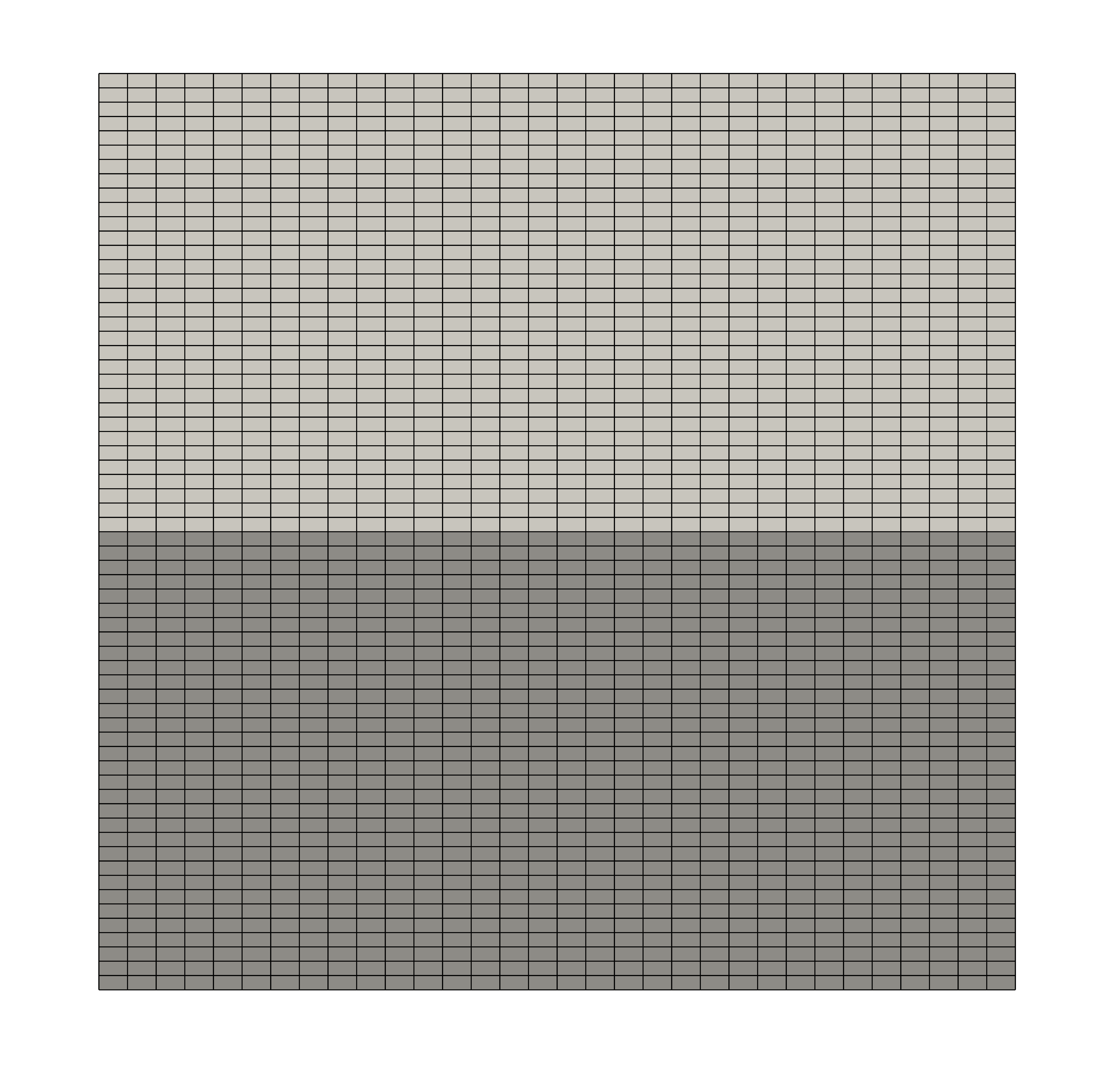
(a) Rectangular piston

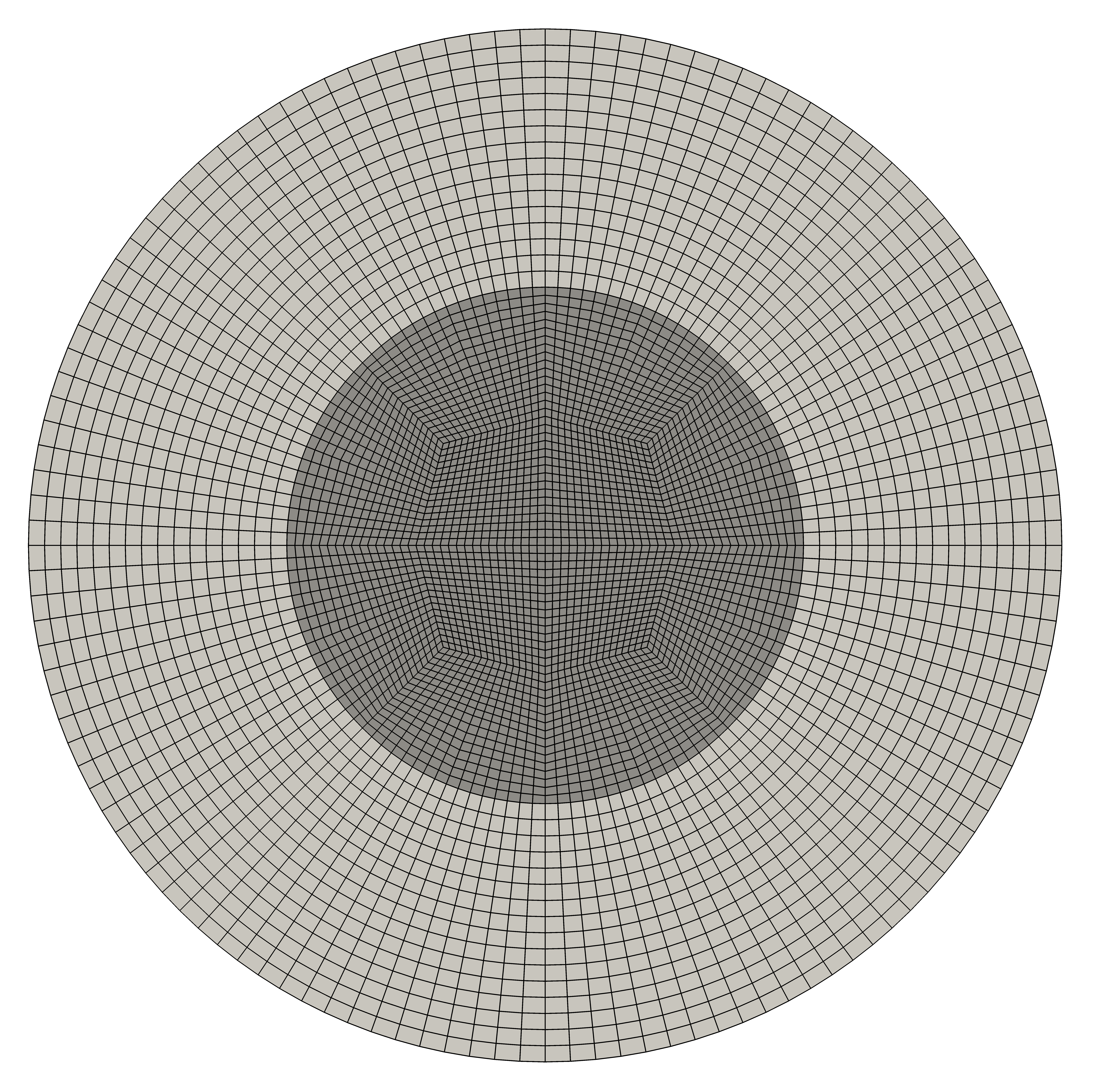
(b) Circular piston

Figure 1: Finite element meshes at refinement level 4 for analytical solutions [94, 95].

The exact solution is defined assuming zero displacements and velocities in horizontal direction and prescribing the vertical component of the interface displacement $\hat{d}_{\Sigma,2}$ as

$$\hat{d}_{\Sigma,2}:=a\sin(\omega t)\qquad\text{with}\quad a:=2\alpha\sin\left(\frac{\omega H}{c_{p}}\right),\quad c_{p}=\sqrt{\frac{\lambda_{s}+2\mu_{s}}{\rho_{s}}},$$ (66)

which oscillates vertically with amplitude $a$ and frequency $\omega$. The structural displacements are thus given by

$$\hat{d}_{s,2}(\hat{x}_{2},t)={f}\left(t-\frac{\hat{x}_{2}+H}{c_{p}}\right)-{f}\left(t+\frac{\hat{x}_{2}+H}{c_{p}}\right)\qquad\text{with }\quad{f}(\tau)=\alpha\cos(\omega\tau)\,.$$

The fluid’s vertical velocity resulting from the continuity equation is solely dependent on time, $u_{f,2}(t)=\frac{\partial}{\partial t}\hat{d}_{\Sigma,2}(t)$, and the pressure is given by

$$p_{f}(x_{2},t)=\frac{(H-x_{2})p_{\Sigma}+(x_{2}-\hat{d}_{\Sigma,2})p_{H}}{H-d_{\Sigma,2}}\qquad\text{with}\quad p_{\Sigma}=-(\lambda_{s}+2\mu_{s})\frac{\partial}{\partial\hat{x}_{2}}\hat{d}_{s,2}(0,t)$$

$$\text{and}\quad p_{H}=-\rho_{f}\left[H-\hat{d}_{s,2}(0,t)\right]\frac{\partial^{2}}{\partial t^{2}}\hat{d}_{s,2}(0,t)+(\lambda_{s}+2\mu_{s})\frac{\partial}{\partial\hat{x}_{2}}\hat{d}_{s,2}(0,t).$$

We refer to the original publications [94, 95] for details on the derivation and proceed in defining problem parameters. The fluid density and dynamic viscosity are set to $\rho_{f}=1\text{\leavevmode\nobreak\ kg/m${}^{3}$}$ and $\mu_{f}\equiv\eta_{\infty}=0.1\text{\leavevmode\nobreak\ Pa\leavevmode\nobreak\ s}$, respectively. For the linear elastic solid we assign the density $\rho_{s}=100\text{\leavevmode\nobreak\ kg/m${}^{3}$}$, the Young’s modulus $E_{s}=5\leavevmode\nobreak\ \text{kPa}$ and a Poisson’s ratio of $\nu_{s}=0.3$. Additionally, we choose $a=0.005$ and $\omega=\pi$ to prescribe the piston motion and enforce Dirichlet conditions on all exterior boundaries of the solid domain, $\hat{\Gamma}_{{D,s}}=\partial\hat{\Omega}_{s}\setminus\hat{\Sigma}$. In terms of boundary conditions for the fluid, we prescribe Neumann conditions at $x_{1}=0$ and $x_{1}=L$ and Dirichlet conditions at $x_{2}=H/2$. Convergence rates are measured in the maximum $L^{2}$-error over all time steps $n=1,...,N_{t}$ for $\text{\boldmath${u}$}_{f}$, $p_{f}$ and $\text{\boldmath${d}$}_{s}$ defined as

$$e_{\text{\boldmath${u}$}_{f}}:=\max_{n=1,...,N_{t}}\left\{||\text{\boldmath${u}$}_{f}-\text{\boldmath${u}$}_{f}^{h}||_{L^{2}(\Omega_{f}^{t})}\right\}\,,\quad e_{p_{f}}:=\max_{n=1,...,N_{t}}\left\{||p_{f}-p_{f}^{h}||_{L^{2}(\Omega_{f}^{t})}\right\}\,,\quad e_{\text{\boldmath${d}$}_{s}}:=\max_{n=1,...,N_{t}}\left\{||\text{\boldmath${d}$}_{s}-\text{\boldmath${d}$}_{s}^{h}||_{L^{2}(\hat{\Omega}_{s})}\right\}\,,$$

and compared to the estimated order of convergence ($eoc$) indicated by triangles in the plots. For the spatial discretisation, equal-order $Q_{1}/Q_{1}$ elements are employed, meaning that $d$-linear shape functions are used for velocities and displacements in both fluid and solid together with $d$-linear elements for the fluid viscosity $\mu_{f}$, fluid pressure $p_{f}$, the variable $\psi$ used for divergence suppression and corresponding traces for $\zeta$. For $t\in(0,0.5]$ we choose uniform time steps and the second-order scheme, i.e., using BDF-$2$, linear extrapolation and the generalised-$\alpha$ schemes with parameters set according to Table 1. Regarding the coupling scheme, we focus first on the classical DN approach with Aitken’s relaxation, implicitly coupling fluid and solid phase. To disentangle the various variants, we introduce them layer by layer and investigate thoroughly the consequences of each change, aiming for the most efficient overall scheme. Starting off, we compare different settings in the generalised-$\alpha$ time integrators.

When refining the time step, expected convergence rates are observed in all primary variables when using the Newmark-$\beta$ scheme, as can be seen in Figure 2.

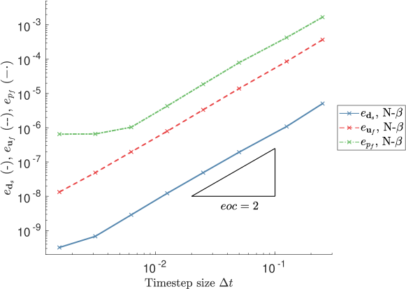
Figure 2: Newmark-$\beta$ time integration with implicit DN coupling yields the expected second-order convergence in time in solid displacements, fluid velocities and pressure.

However, when introducing numerical high-frequency dissipation via the generalised-$\alpha$ time integration scheme with a spectral radius in the high frequency limit $\rho_{\infty}\neq 1$, an increase in the saturation error as exemplarily shown in Figure 3 for $\rho_{\infty}=0.98$ is observed. Choosing a practically relevant (user-specified) high-frequency dissipation/spectral radius in the high-frequency limit $\rho_{\infty}$, second-order convergence in velocities, displacements and pressure are maintained.

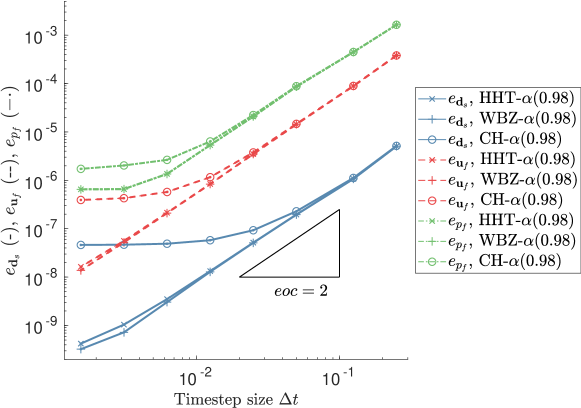
Figure 3: Generalised-$\alpha$ time integration with implicit DN coupling: Choosing a spectral radius in the high frequency limit $\rho_{\infty}=0.98$ results in an increased saturation error compared to $\rho_{\infty}=1.0$ or Newmark-$\beta$ time integration.

A value of $\rho_{\infty}=1$ yields identical results to the N-$\beta$ scheme for the HHT-$\alpha$ and WBZ-$\alpha$, whereas the so-called asymptotic annihilation case, i.e., $\rho_{\infty}=0$, leads to a clearly linear convergence rate in $p_{f}$ for WBZ-$\alpha$ and CH-$\alpha$ methods as can be seen in Figure 4 (and is not admissible for the HHT-$\alpha$ scheme). Again, the earlier error saturation in $e_{\text{\boldmath${d}$}_{s}}$ and $e_{\text{\boldmath${u}$}_{f}}$ is most clearly observed for the CH-$\alpha$ scheme. The decreased convergence rate in the fluid pressure $p_{f}$ is linked to the term $\langle\varphi\text{\boldmath${n}$}_{f},\rho_{f}\ddot{\text{\boldmath${d}$}}_{s}^{n+1}(\text{\boldmath${d}$}_{s}^{k})\rangle_{\Sigma^{t}}$ appearing in the PPE (62), which is for the generalised-$\alpha$ scheme only first order accurate in time if $\alpha_{f}\neq\alpha_{m}$ [126].

Figure 4: Generalised-$\alpha$ time integration with implicit DN coupling and various $\rho_{\infty}$: Increased algorithmic damping as $\rho_{\infty}\rightarrow 0$ results in an increased saturation error and reduces the temporal order of convergence of the fluid pressure from the optimal 2 down to 1.

The fully implicit variant of the RR scheme yields similar results and is thus not further discussed at this point.

Regarding the semi-implicit Dirichlet–Neumann (SIDN) and Robin–Robin (SIRR) coupling schemes, we report the expected convergence rates in Figure 5, treating the mesh motion equation, fluid momentum equation, viscosity projection and divergence suppression explicitly. Additionally, taking the fully implicit N-$\beta$ scheme as a baseline, saturation errors in the fluid pressure increase for both semi-implicit variants. Using the RR coupling scheme, the saturation errors of the fluid pressure and velocity depend on the Robin parameters $\eta_{s}^{R}$ and $\eta_{f}^{R}$ [72]

$$\eta_{f}^{R}=\frac{\rho_{s}H_{s}}{\Delta t}+\beta\Delta t\quad\text{and}\quad\eta_{s}^{R}=\frac{\rho_{f}}{\Delta t}\gamma\mu_{max}\,,$$ (67)

where $H_{s}=1$, $\beta=0$ and $\gamma\mu_{max}=0.01$ were chosen, the latter of which was found uncritical in this example. Considering the substantial increase in efficiency, the semi-implicit schemes are very attractive for practical applications as indicated at various places in the literature [77, 79, 80, 20, 81, 82, 84].

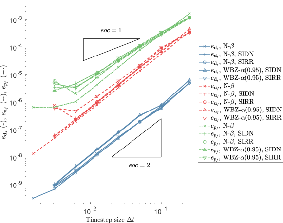
Figure 5: Newmark-$\beta$ and WBZ-$\alpha$ $(\rho_{\infty}=0.95)$ time integration: The semi-implicit SIDN and SIRR schemes yield almost identical errors compared to the fully implicit DN coupling independent of the time integration scheme applied.

4.2 Analytical solution: circular piston

Another analytical solution is employed to confirm the expected convergence rates in space. A circular piston as depicted in Figure 1b, where the structure occupies the region from $\hat{r}=0$ to the interface at $\hat{r}_{\Sigma}=r_{\Sigma}(t=0)$ in the reference configuration, pulsates in radial direction, driving the fluid. For a detailed derivation see [94, 95], whereas herein we conveniently express the solution in terms of the radial component of structure displacement

$$\hat{\text{\boldmath${d}$}}_{s,r}(\hat{r},t):=\beta\mathcal{J}_{1}\left(\frac{\omega\hat{r}}{c_{p}}\right)\sin(\omega t)\,,\quad\text{such that }r_{\Sigma}(t)=r_{\Sigma}^{0}+\hat{\text{\boldmath${d}$}}_{s,r}(r_{\Sigma}^{0},t)$$

with frequency $\omega$, a parameter $\beta$ scaling the amplitude, initial piston radius $r_{\Sigma}^{0}$, $c_{p}$ as defined in Equation (66) and $\mathcal{J}_{1}$ denoting the Bessel function of the first kind and order one, which gives the fluid’s radial velocity component

$$\text{\boldmath${u}$}_{f,r}(r,t)=\frac{R}{r}V(t)\,,\quad\text{with}\quad V(t)=\frac{\omega\beta}{R}r_{\Sigma}(t)\mathcal{J}_{1}\left(\frac{\omega r_{\Sigma}^{0}}{c_{p}}\right)\cos(\omega t)\,,$$

and the fluid pressure

$$p_{f}(r,t)= P(t)+\frac{\rho_{f}}{2}\left[1-\left(\frac{R}{r}\right)^{2}\right]V(t)^{2}+\rho_{f}R\log\left(\frac{R}{r}\right)\frac{\partial}{\partial t}V(t)\,,$$

$$\text{with }P(t)= -\frac{\rho_{f}}{2}\left[1-\left(\frac{R}{r_{\Sigma}(t)}\right)^{2}\right]V(t)^{2}-\rho_{f}R\log\left(\frac{R}{r_{\Sigma}(t)}\right)\frac{\partial}{\partial t}V(t)$$

$$-\beta\sin(\omega t)\left[(\lambda_{s}+2\mu_{s})\frac{\omega}{c_{p}}\mathcal{J}_{1}^{\prime}\left(\frac{\omega r_{\Sigma}^{0}}{c_{p}}\right)+\frac{\lambda_{s}}{r_{\Sigma}^{0}}\mathcal{J}_{1}\left(\frac{\omega r_{\Sigma}^{0}}{c_{p}}\right)\right]\,,$$

where $\mathcal{J}_{1}^{\prime}$ denotes the first derivative of $\mathcal{J}_{1}$. The piston with initial radius $r_{\Sigma}^{0}=0.5$ pulsates with frequency $\omega=\pi$ and $\beta=0.1$ is set. Fluid’s density and dynamic viscosity are considered as $\rho_{f}=1\text{\leavevmode\nobreak\ g/m${}^{3}$}$ and $\mu_{f}=\eta_{\infty}=0.5\text{\leavevmode\nobreak\ mPa\leavevmode\nobreak\ s}$, respectively. The linear-elastic solid has a density of $\rho_{s}=1\text{\leavevmode\nobreak\ kg/m${}^{3}$}$, a Young’s modulus of $E_{s}=100\text{\leavevmode\nobreak\ kPa}$ and a Poisson’s ratio of $\nu_{s}=0.3$. To minimise the influence of time integration error, the time interval from $t=0$ to $t=0.05\leavevmode\nobreak\ \text{s}$ is divided into $80$ equal time steps of constant length $\Delta t=0.625\leavevmode\nobreak\ \text{ms}$ and integrated using second-order time-stepping schemes and extrapolation.

The experimental orders of convergence are reported in Figure 6, allowing for a direct comparison of the errors obtained with $Q_{2}/Q_{1}$ and $Q_{1}/Q_{1}$ elements and various coupling schemes, where the Robin parameters are again set according to (67). The deliberately chosen parameters result in directly recovering the exact solution of $\text{\boldmath${d}$}_{s}$ up to the specified tolerance/time integration error, but allow easily measuring experimental convergence rates of fluid velocity and pressure. The fluid velocities converge at a rate of $eoc=2$ for the fully implicit and semi-implicit schemes with almost identical errors obtained. This is exactly as expected, even for the $Q_{2}/Q_{1}$ finite element pairing (cf. [103, 102, 110]). Pressure rates of order $1$ are observed for linear pressure interpolation and a slightly higher rate of $eoc\approx 1.5$ when using $Q_{2}/Q_{1}$ interpolation. These results are optimal for the considered split-step scheme in the fluid pressure, where one might expect convergence rates of order $1$ using (bi-)linear elements in the observed norm. However, the measured rates of $\approx 1.5$ for the $Q_{2}/Q_{1}$ pair are lower than what one would hope for, judging from the basic split-step scheme, which gives rates of $2$ in the pressure norm observed here. These higher rates are found initially, but decrease under refinement. Additionally, the solid subproblem yielded optimal convergence rates when tested using different parameter settings, which is omitted for the sake of brevity. The sole reason for not choosing those different parameter settings altogether is the inherent difficulty in demonstrating all convergence rates at the same time, which was not found possible here due to the problem setup and relative sizes of physical quantities and tolerance choices.

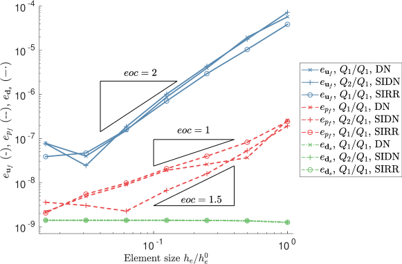
Figure 6: Spatial convergence rates obtained using $Q_{1}/Q_{1}$ or $Q_{2}/Q_{1}$ interpolation in combination with the DN coupling scheme or semi-implicit variants SIDN and SIRR.

4.3 Pressure pulse benchmark

To investigate the influence of different material models on the coupling algorithm, we consider a variant of the well-established benchmark example of a pressure pulse traveling through a straight flexible tube as used in [96] based on [111, 66]. The parameter choice is inspired by hemodynamic applications, fixing the tube length of $l=5\leavevmode\nobreak\ \text{cm}$ and inner radius of $r_{\text{i}}=0.5\leavevmode\nobreak\ \text{cm}$. The surrounding solid is divided into two layers $\hat{\Omega}_{s,1}$, $\hat{\Omega}_{s,2}$ of equal thickness $h_{s}=0.05\leavevmode\nobreak\ \text{cm}$ indicated by different colors in Figure 7a, resulting in an outer radius of $r_{\text{o}}=0.6\leavevmode\nobreak\ \text{cm}$.

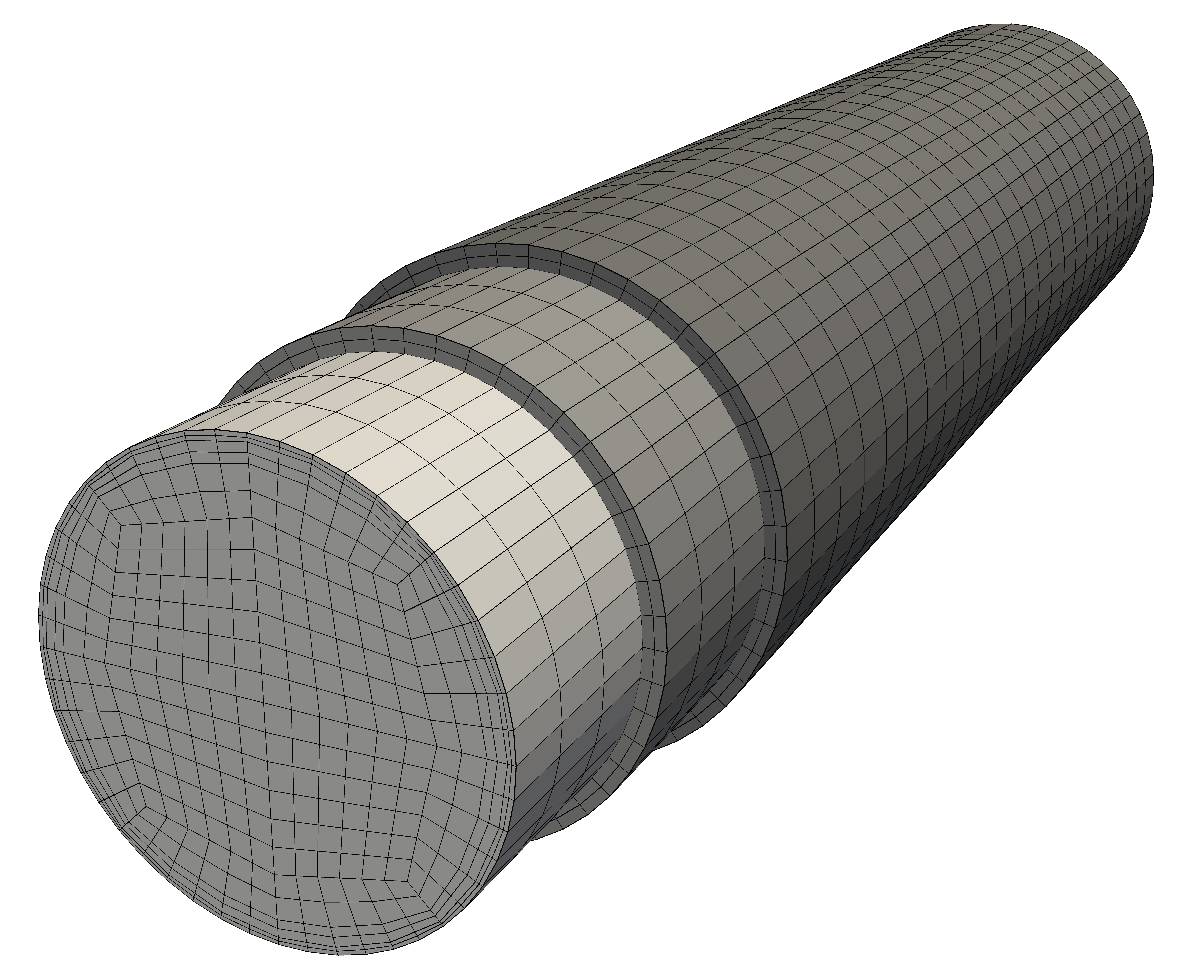
(a) Fluid mesh with boundary layers and cut solid domains resolving medial and adventitial tissue layers.

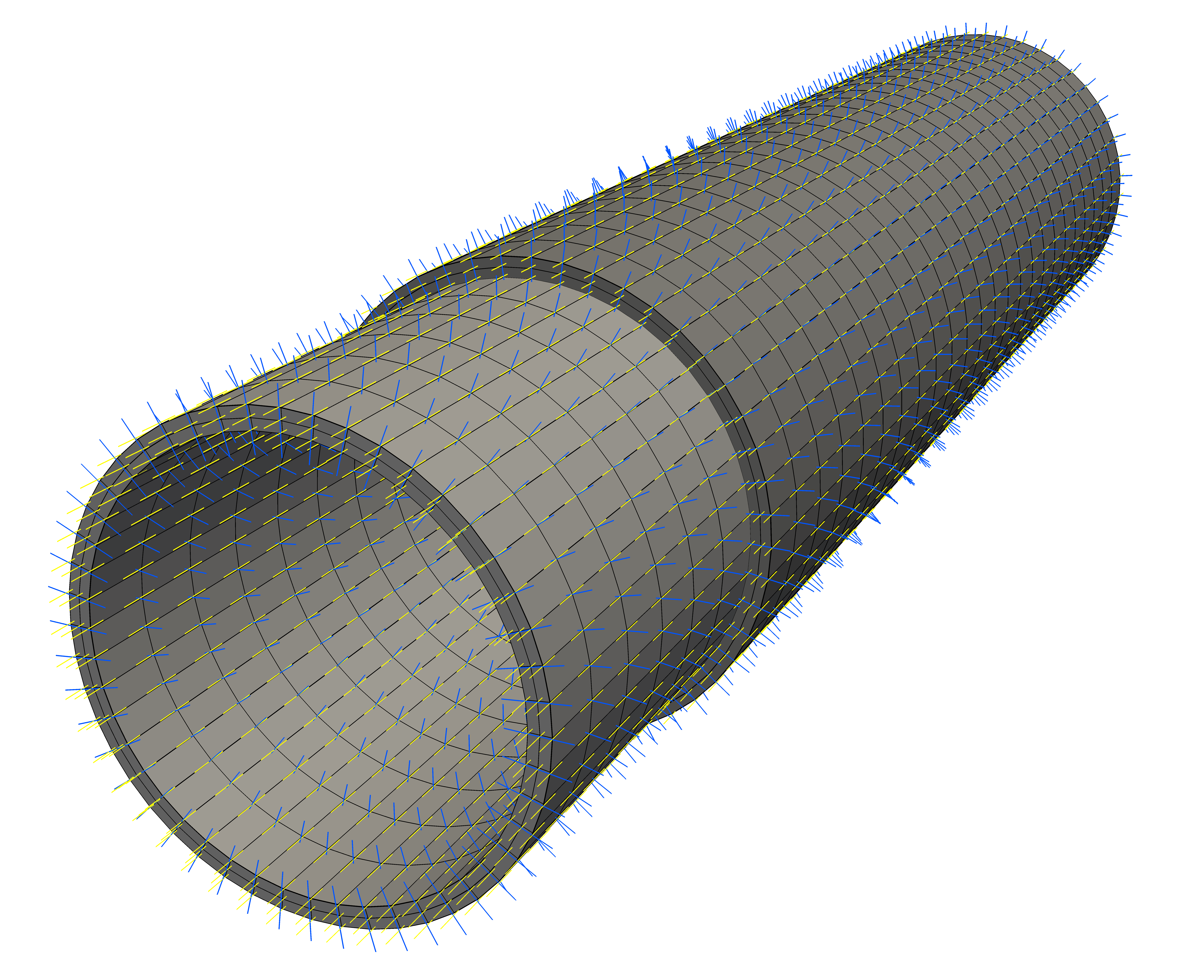
(b) Radial (blue) and longitudinal (yellow) orientation vectors in cut solid domains used to construct $\hat{\text{\boldmath${e}$}}_{1}$ and $\hat{\text{\boldmath${e}$}}_{2}$.

Figure 7: Finite element mesh considered for the pressure pulse benchmark.

A pressure pulse is generated setting $\text{\boldmath${\sigma}$}_{f}\text{\boldmath${n}$}_{f}=-p_{\mathrm{in}}\text{\boldmath${n}$}_{f}$ at the inlet, with $p_{\mathrm{in}}=10\leavevmode\nobreak\ \text{mmHg}\approx 1333.22\leavevmode\nobreak\ \text{Pa}$ for the first $9\leavevmode\nobreak\ \text{ms}$ and zero otherwise. On the outflow boundary, zero Neumann conditions are enforced. The tube is fixed at both ends, and zero traction conditions are prescribed at the solid’s external boundary at $r=r_{o}$. Effects of external tissue support and downstream vasculature are neglected at this point, but can be introduced easily using lumped parameter models [111, 142, 143, 144, 145, 146, 147]. Concerning the material parameters, we set the fluid and solid densities to $\rho_{s}=1200\leavevmode\nobreak\ \text{kg/m${}^{3}$}$ and $\rho_{f}=1060\leavevmode\nobreak\ \text{kg/m${}^{3}$}$, which triggers strong added-mass effects. Further, we consider a Newtonian fluid with a viscosity of $\mu_{f}=3.5\leavevmode\nobreak\ \text{mPa\leavevmode\nobreak\ s}$, which needs to be suitably chosen (see, e.g., [148, 96, 149]) for comparison to the more general Carreau model with $\eta_{0}=56\leavevmode\nobreak\ \text{mPa\leavevmode\nobreak\ s}$, $\eta_{\infty}=3.45\leavevmode\nobreak\ \text{mPa\leavevmode\nobreak\ s}$, $\lambda_{f}=3.313\leavevmode\nobreak\ \text{s}$ and $n=0.3568$ taken from [150]. For the solid phase, linear elasticity (11) or a St. Venant–Kirchhoff solid (10), both with Young’s modulus $E_{s}=300\leavevmode\nobreak\ \text{kPa}$ and Poisson ratio $\nu_{s}=0.3$ are compared to layered models of neo-Hookean material with and without additional fiber reinforcement (Equations (12) and (13)). The latter two choices use $\nu_{s}=0.499$ and shear rates of $\mu_{s,1}=62.1\leavevmode\nobreak\ \text{kPa}$ and $\mu_{s,2}=21.6\leavevmode\nobreak\ \text{kPa}$ for the inner and outer layers, respectively. Fiber parameters are chosen as $k_{1}=1.4\leavevmode\nobreak\ \text{kPa}$, $k_{2}=22.1$ and $\kappa_{c,1}=0.12$, $\alpha_{c,1}=27.47^{\circ}$ or $\kappa_{c,2}=0.25$, $\alpha_{c,2}=52.88^{\circ}$ in inner and outer layers according to [151, 152, 153].

We use a uniform time step of $\Delta t=0.5\leavevmode\nobreak\ \text{ms}$ in the second-order accurate scheme, i.e., BDF-2 and linear extrapolation as initial guess or possible linearisation. The WBZ$-\alpha$ and CH$-\alpha$ time integrators with $\rho_{\infty}=0$ are selected to counteract pressure oscillations in time caused by the jump in the Neumann condition and simultaneously give the lowest iteration counts. Aitken’s relaxation is initiated with $\omega_{0}=0.01$, coupling the subproblems until reaching $\epsilon_{abs}=10^{-7}$ or $\epsilon_{rel}=10^{-4}$, while a relative Newton tolerance of $\epsilon_{N}=10^{-3}$ in (19) was found sufficient.

Snapshots of the travelling pulse are shown in Figure 8, where the HGO and Carreau models were employed. As opposed to the traditional benchmark, the hemodynamic-inspired setting features larger displacements given the lower material stiffness, as can be seen in Figure 9a. However, despite the maximum displacement being $\approx 30$ % of the tube’s thickness (and also only $\approx 0.6$% of the tube’s length), strains are small enough for linear elasticity (E) and St. Venant–Kirchhoff (SVK) solid to yield almost identical values for both the observed quantities (see Figures 9a and 9b). The fiber contribution present in the HGO model is already visible, but not dominant given the fiber parameters and small strains. Comparing the different rheological laws used, one can see large variations in viscosity at any point in time (see Figure 8), but negligible effects on displacements and pressure. Additionally, we observe “backflow” instabilities as a consequence of fluid entering over the inlet Neumann boundary due to mass conservation. Despite those oscillations close to the inlet, the solver still converges. Possible remedies to stabilise such effects are backflow stabilisation or similar techniques [142, 154, 146, 111, 155, 156], which are not considered at this point.

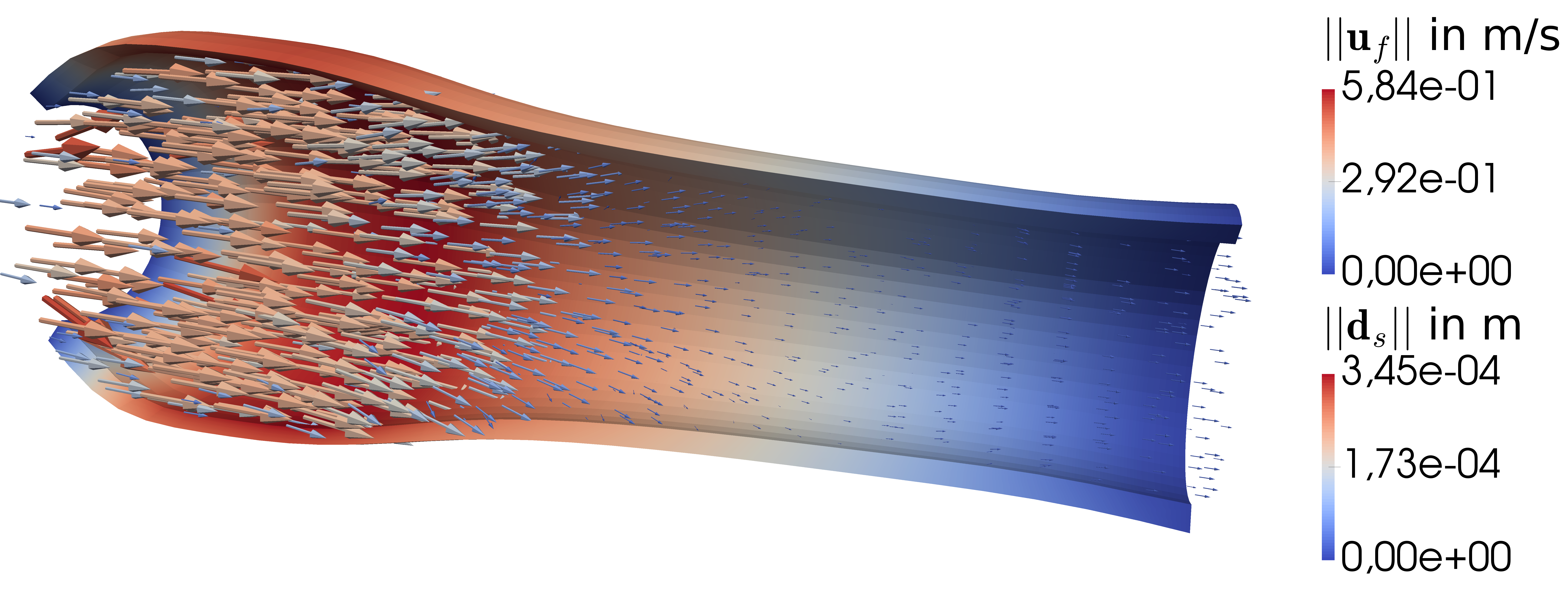
(a) $\text{\boldmath${d}$}_{s}$ and $\text{\boldmath${u}$}_{f}$ at $t=15\leavevmode\nobreak\ \text{ms}$.

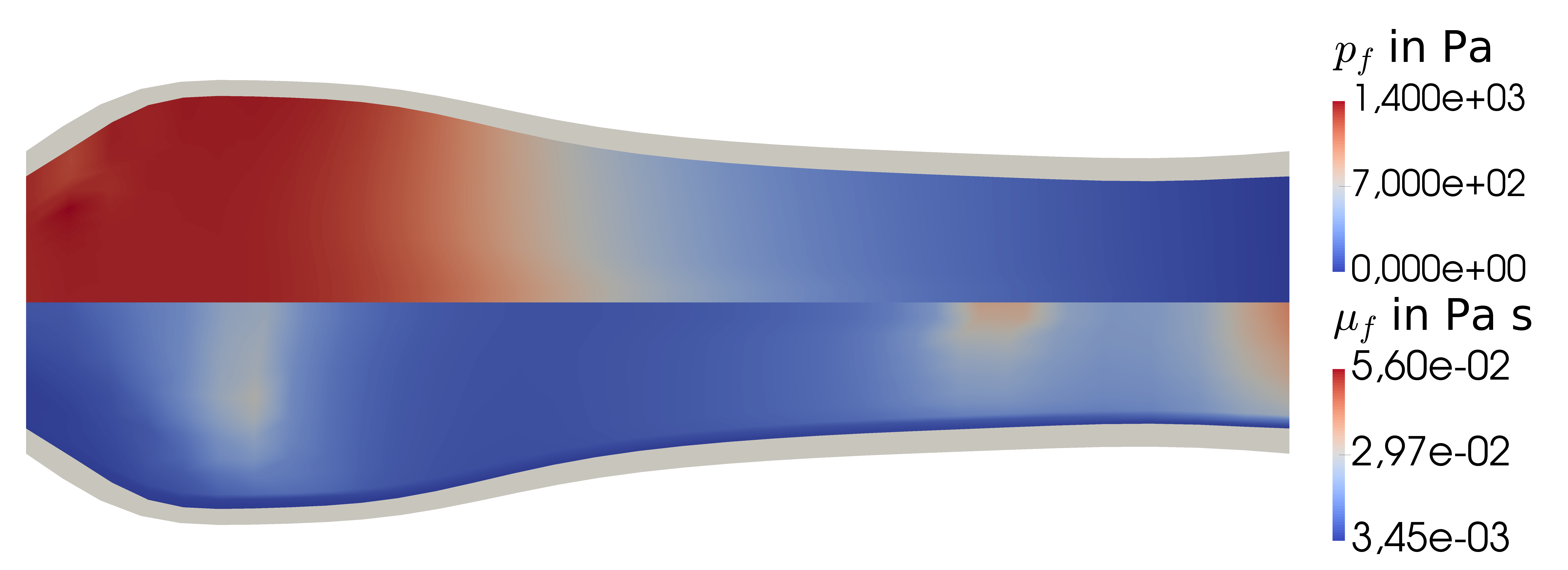
(b) $p_{f}$ (top) and $\mu_{f}$ (bottom) at $t=15\leavevmode\nobreak\ \text{ms}$.

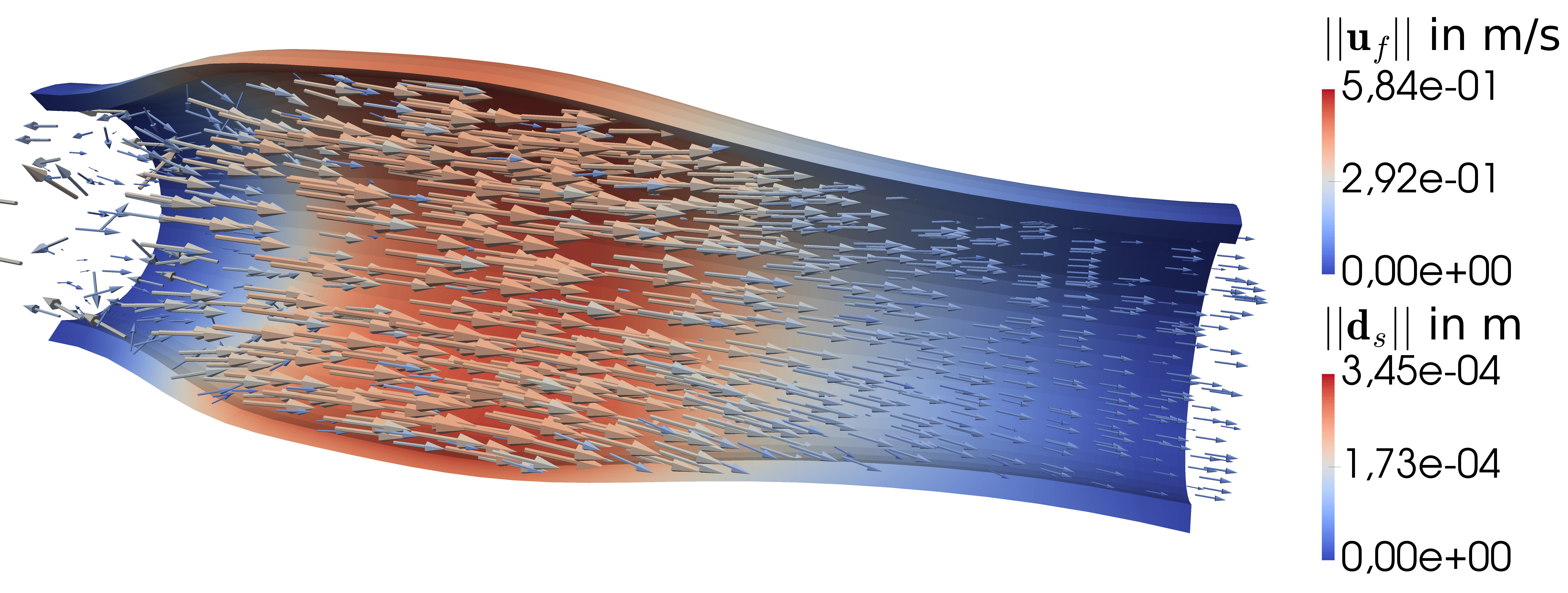
(c) $\text{\boldmath${d}$}_{s}$ and $\text{\boldmath${u}$}_{f}$ at $t=22\leavevmode\nobreak\ \text{ms}$.

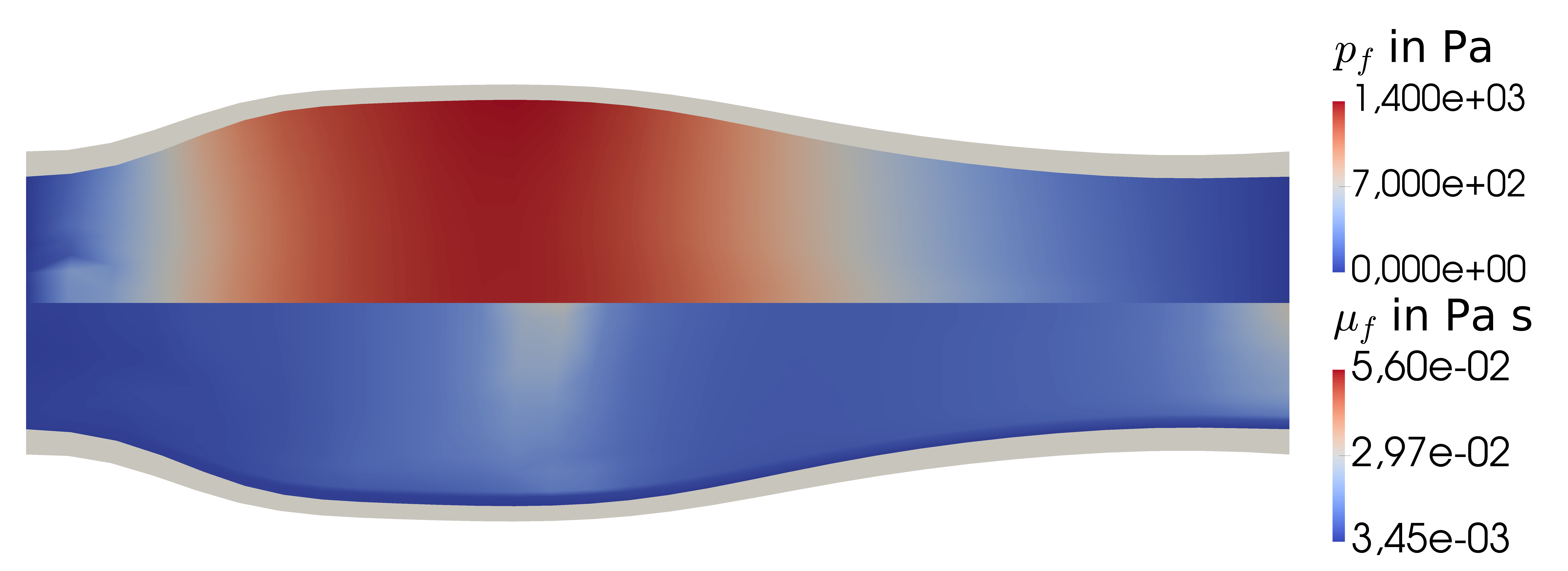
(d) $p_{f}$ (top) and $\mu_{f}$ (bottom) at $t=22\leavevmode\nobreak\ \text{ms}$.

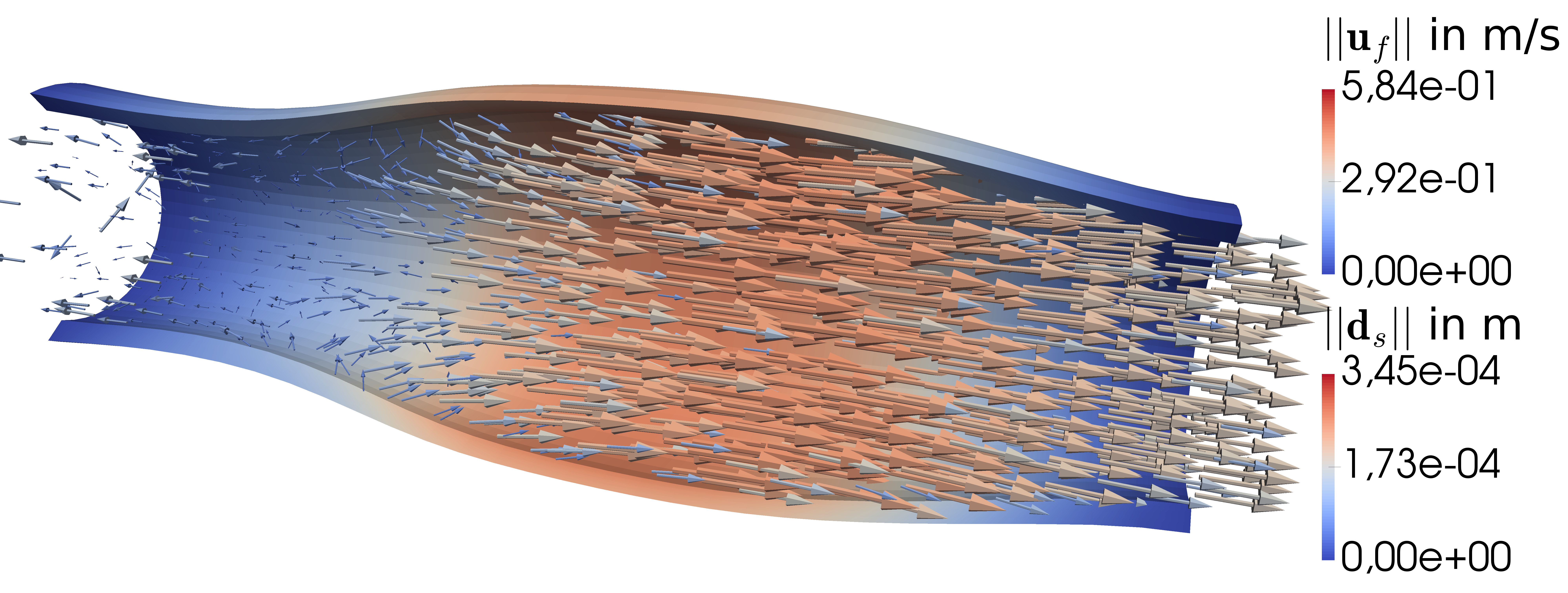
(e) $\text{\boldmath${d}$}_{s}$ and $\text{\boldmath${u}$}_{f}$ at $t=29\leavevmode\nobreak\ \text{ms}$.

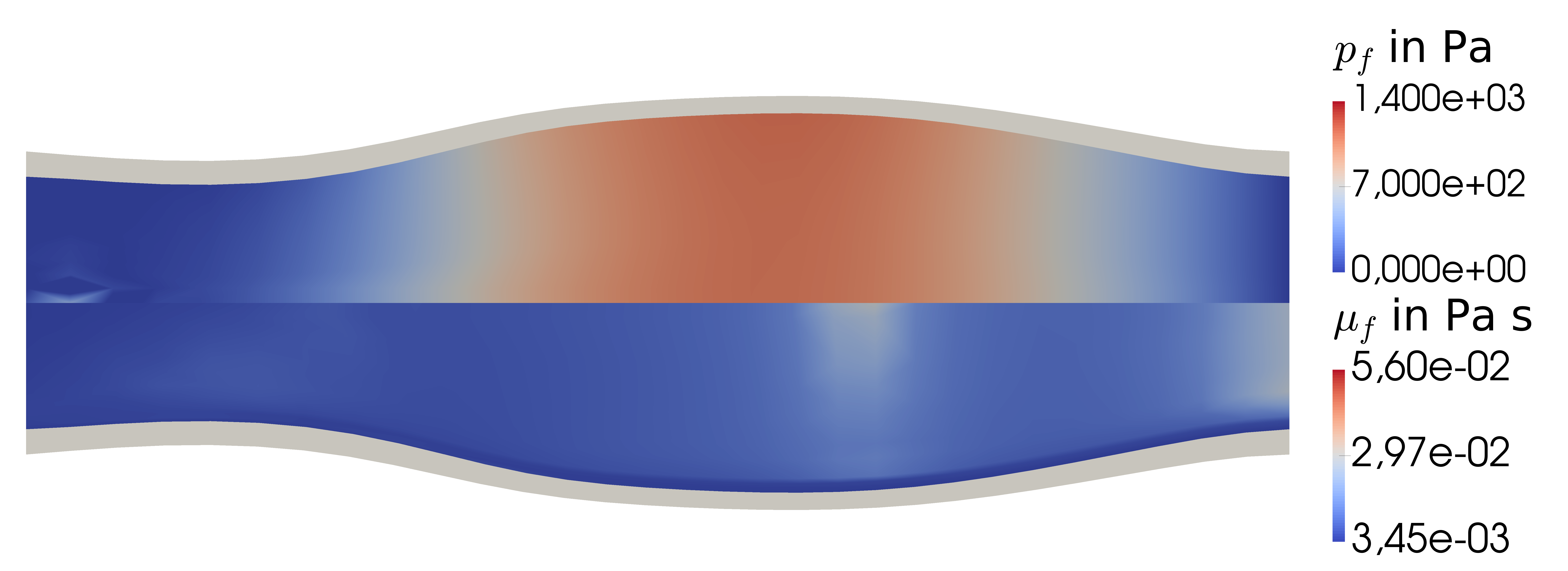
(f) $p_{f}$ (top) and $\mu_{f}$ (bottom) at $t=29\leavevmode\nobreak\ \text{ms}$.

Figure 8: Snapshots at time $t=15,22,29\leavevmode\nobreak\ \text{ms}$ of the pressure pulse in the Carreau fluid traveling the tube of HGO material (deformation scaled by $10$): Solid displacement $\text{\boldmath${d}$}_{s}$ and fluid velocity $\text{\boldmath${u}$}_{f}$ in cut tube (left), pressure $p_{f}$ and viscosity $\mu_{f}$ in slice at $x_{2}=0$ (right).

(a) Displacement comparison.

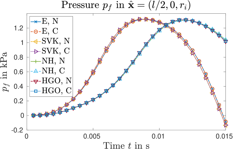
(b) Pressure comparison.

Figure 9: Pressure-pulse benchmark with linear elasticity (E), St. Venant–Kirchhoff (SVK), neo-Hookean (NH) or Holzapfel–Gasser–Ogden (HGO) material models for the solid phase and Newtonian (N) or Carreau (C) fluids.

Let us note here that the presented solutions can merely indicate that suitable parameters and material laws themselves are central aspects in the description of the system behavior. This, however, does not lie within the scope of this contribution, since the aim here is simply to demonstrate versatility by easily switching between constitutive equations of particular interest depending on the available data or application. Within this work, we present this problem setup to assess computational performance of the various coupling schemes presented. From now on, we only consider linear elasticity with a Newtonian fluid and the HGO model together with the Carreau law.

Inspecting the accumulated FSI iterations depicted in Figure 10, we see that the total iteration counts are decreasing with the semi-implicit schemes. Interestingly, treating the fluid mesh motion and momentum balance equations explicitly does not only reduce the computational cost of one individual coupling step, but also reduces the number of total iterations. This effect is independent of the material laws applied, potentially boosting computational performance depending on the fluid and solid subproblem sizes. But on the flip side of the coin, we rather surprisingly see that the Robin–Robin variants of the scheme do not improve convergence in contrast to the results presented in [79, 72]. In those papers, the Robin condition on the fluid phase was found to substantially decrease the number of needed coupling steps, which does not seem to transfer to the present split-step approach. To diminish a possible influence of the Robin parameter, tests are conducted in the linear elasticity/Newtonian fluid case varying the Robin parameters in the fluid momentum balance and PPE. The latter option modifies Equations (61) and (62) to include Robin interface conditions as well, but was found diverging for any $\eta_{f}^{R}$. Scaling the Robin parameter $\eta_{f}^{R}$ computed via Equation (67) in the fluid momentum balance by some $\alpha_{R}$, iteration counts stay almost identical for $\alpha_{R}$ large enough, as can be seen in Figure 11. Choosing $\alpha_{R}\rightarrow 0$ and $\alpha_{R}\rightarrow\infty$ correspond to Neumann–Neumann and the standard Dirichlet–Neumann coupling schemes, first of which needs more than the preset maximum of 150 steps to converge leading to divergence in the fifth time step.

The Robin parameter $\eta_{s}^{R}$ in the solid’s balance of linear momentum has two distinct interpretations depending on the coupling scheme applied: in implicit schemes, a standard Robin–Robin coupling is recovered, possibly mildly increasing efficiency as reported by Badia et al. [72]. In our semi-implicit scheme, however, it is recalled that the interface Robin term is responsible for information transfer from fluid to solid phase (with $n$ indicating the time step, $k$ the iterate in the FSI coupling scheme and $l$ the iterate in Newton’s method) as

$$\alpha_{f}^{\prime}\langle\text{\boldmath${\varphi}$},\text{\boldmath${P}$}(\text{\boldmath${d}$}_{s}^{n+1}){\hat{\text{\boldmath${n}$}}}_{s}\rangle_{\hat{\Sigma}}= \alpha_{f}^{\prime}\langle\text{\boldmath${\varphi}$},\text{\boldmath${h}$}_{s}^{n+1}-\eta_{s}^{R}\dot{\text{\boldmath${d}$}}_{s}^{n+1}(\text{\boldmath${d}$}_{s}^{l})\rangle_{\hat{\Sigma}}$$

$$= \alpha_{f}^{\prime}\langle\text{\boldmath${\varphi}$},\eta_{s}^{R}\text{\boldmath${u}$}_{f}^{k}+J_{f}^{k}\text{\boldmath${\sigma}$}(\text{\boldmath${u}$}_{f}^{k},p_{f}^{k+1},\mu_{f}^{k+1})\text{\boldmath${F}$}_{\!f}^{-T}{\hat{\text{\boldmath${n}$}}}_{s}-\eta_{s}^{R}\dot{\text{\boldmath${d}$}}_{s}^{n+1}(\text{\boldmath${d}$}_{s}^{l})\rangle_{\hat{\Sigma}},$$

which as $\eta_{s}^{R}\rightarrow 0$ reduces to a Neumann condition on the interface, but as $\eta_{s}^{R}\rightarrow\infty$ smoothly transitions to an explicit coupling scheme based on the extrapolated velocity $\text{\boldmath${u}$}_{f}^{k}$. Despite the latter greatly decreasing the number of coupling iterations depending on the specific choice for $\eta_{s}^{R}$, one also observes decreased temporal stability. Therefore, $\eta_{f}^{R}=10^{2}\frac{\rho_{s}}{\Delta t}$ and $\eta_{s}^{R}=10^{-4}\frac{\rho_{f}}{\Delta t}$ are chosen for all of the RR results presented in Figure 10.

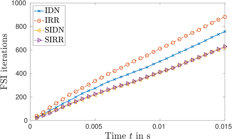
(a) Linear Elasticity, Newtonian fluid.

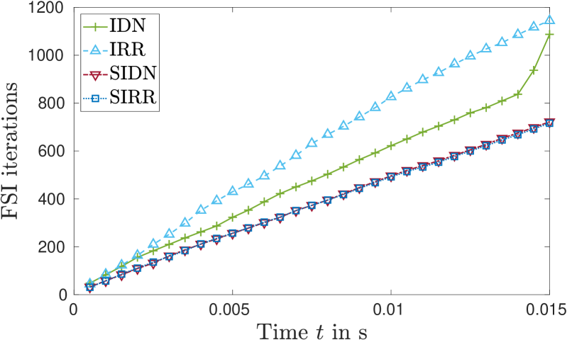
(b) HGO model, Carreau fluid.

Figure 10: Accumulated FSI iterations using implicit Dirichlet–Neumann (IDN) or Robin–Robin (IRR) variants and semi-implicit counterparts (SIDN, SIRR) in the pressure pulse benchmark.

Before moving on to a final, more challenging example, let us summarise the insights gained from this simple pressure pulse benchmark: As expected, semi-implicit treatment of both the fluid mesh motion and fluid balance of linear momentum is found sufficiently accurate, while the constitutive equations considered for fluid and solid phases can be exchanged effortlessly similar to other partitioned approaches. In this simple setup, however, neither the generalised Newtonian rheology nor the nonlinear contributions, which differentiate linear elasticity from the St. Venant–Kirchhoff model or the fiber reinforcement in the HGO model compared to the neo-Hookean one, change the observed quantities much. Moreover, introducing Robin conditions in the framework did not improve convergence properties, only mild improvements are seen in some cases, but instabilities arise from unsuitable choices. The semi-implicit Robin–Robin or Dirichlet–Robin schemes transition to fully explicit schemes as $\eta_{s}^{R}\rightarrow\infty$, which are found rather unstable in first numerical tests. Consequently, the method of choice is the SIDN algorithm, which delivered low iteration counts, stable solutions and requires less data transfer than the Robin variants.

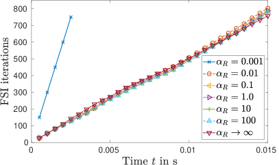
Figure 11: Accumulated FSI iterations using implicit Robin–Neumann coupling with Robin parameter $\eta_{f}^{R}=\alpha_{R}\frac{\rho_{s}}{\Delta t}$, linear elasticity and a Newtonian fluid in the pressure pulse benchmark.

4.4 Flow through an idealised aneurysm

In this final numerical example, we consider the flow through an idealised abdominal aortic aneurysm (AAA) using physiological parameter sets to challenge the devised framework. The setup chosen is similar to [157], combining a prototypical geometry as recommended by surgeons [158, 159] with flow data from [160]. Comparable settings in a biomedical context with benchmark character were presented by Turek et al. [161] and Balzani et al. [162], while patient-specific geometries were considered, e.g., in [53, 10, 163].

The AAA geometry with a length of $l=20\leavevmode\nobreak\ \text{cm}$ and with inner/lumen radius of $r_{i}=1\leavevmode\nobreak\ \text{cm}$ at the in- and outlet is discretised using $\approx 1.3\times 10^{5}$ trilinear elements as depicted in Figure 12, resulting in $\approx 1.3\times 10^{5}$ nodes. These radii are expanded to a maximum of $\approx 6.5\leavevmode\nobreak\ \text{cm}$ in lateral direction and $\approx 5.5\leavevmode\nobreak\ \text{cm}$ in anterior-posterior direction in the middle of the aneurysm. , $\hat{\Omega}_{s,1}$ and $\hat{\Omega}_{s,2}$, are considered with a uniform and equal thickness of $h_{s}=0.75\leavevmode\nobreak\ \text{mm}$, where a fiber orientation is constructed by solving two auxiliary Laplace equations as in the pressure pulse benchmark and . The computational domain is distributed to 8 processors as indicated by different colors in Figure 13a, ignoring the fluid structure interface.

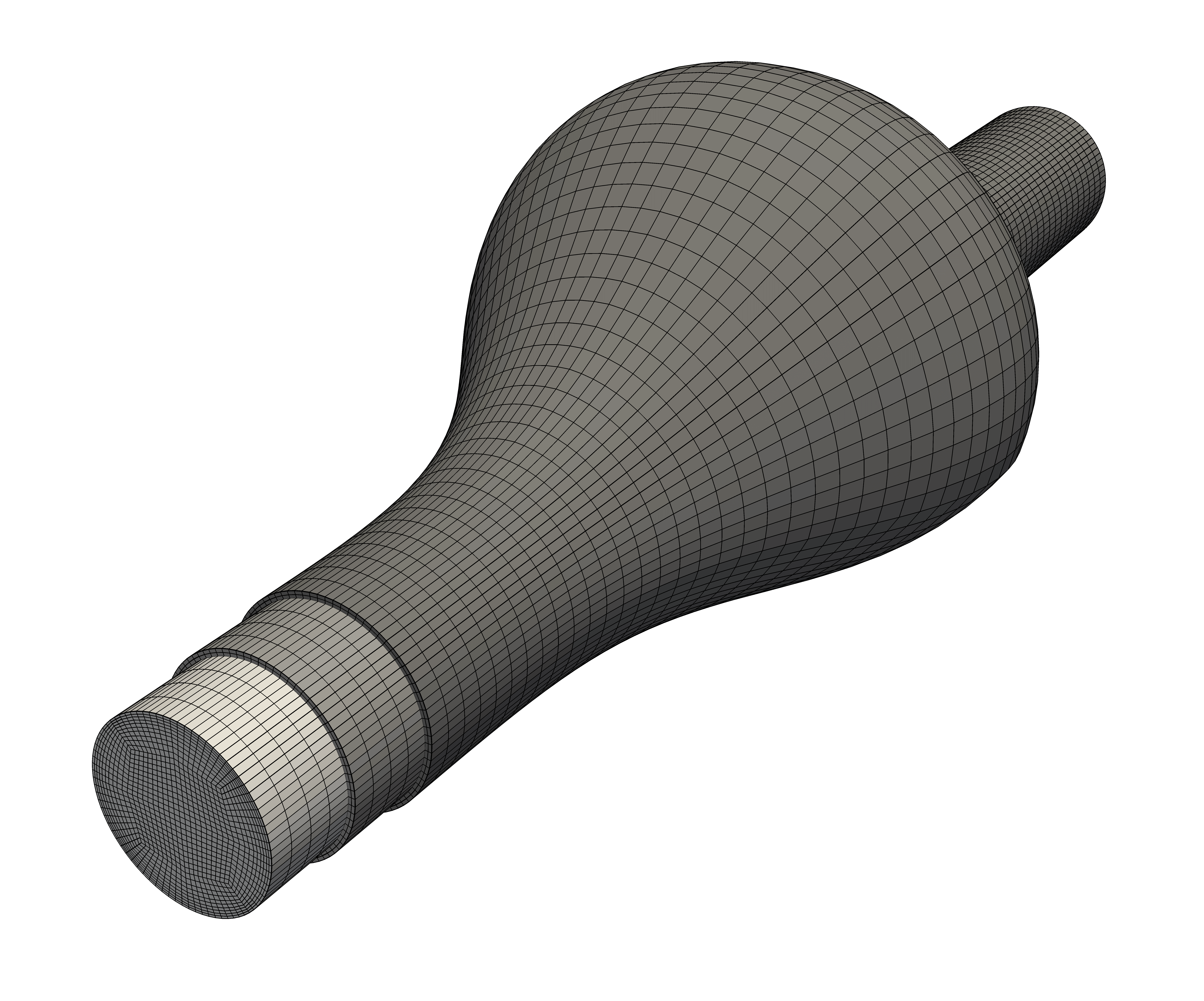
(a) Fluid mesh with boundary layers and cut solid domains resolving medial and adventitial tissue layers.

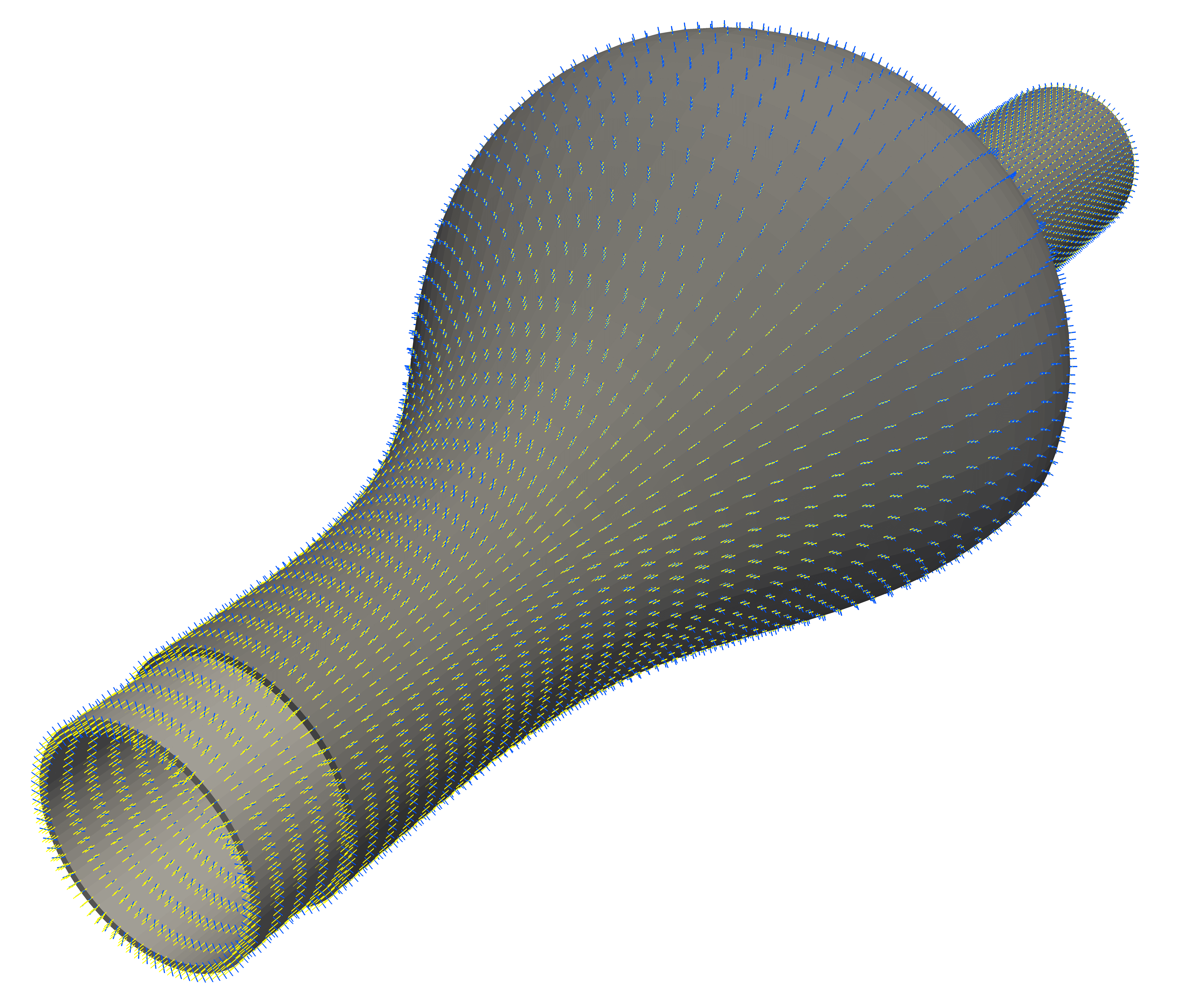
(b) Radial (blue) and longitudinal (yellow) orientation vectors in cut solid domains used to construct $\hat{\text{\boldmath${e}$}}_{1}$ and $\hat{\text{\boldmath${e}$}}_{2}$.

Figure 12: Finite element mesh used in the idealised abdomial aortic aneurysm example.

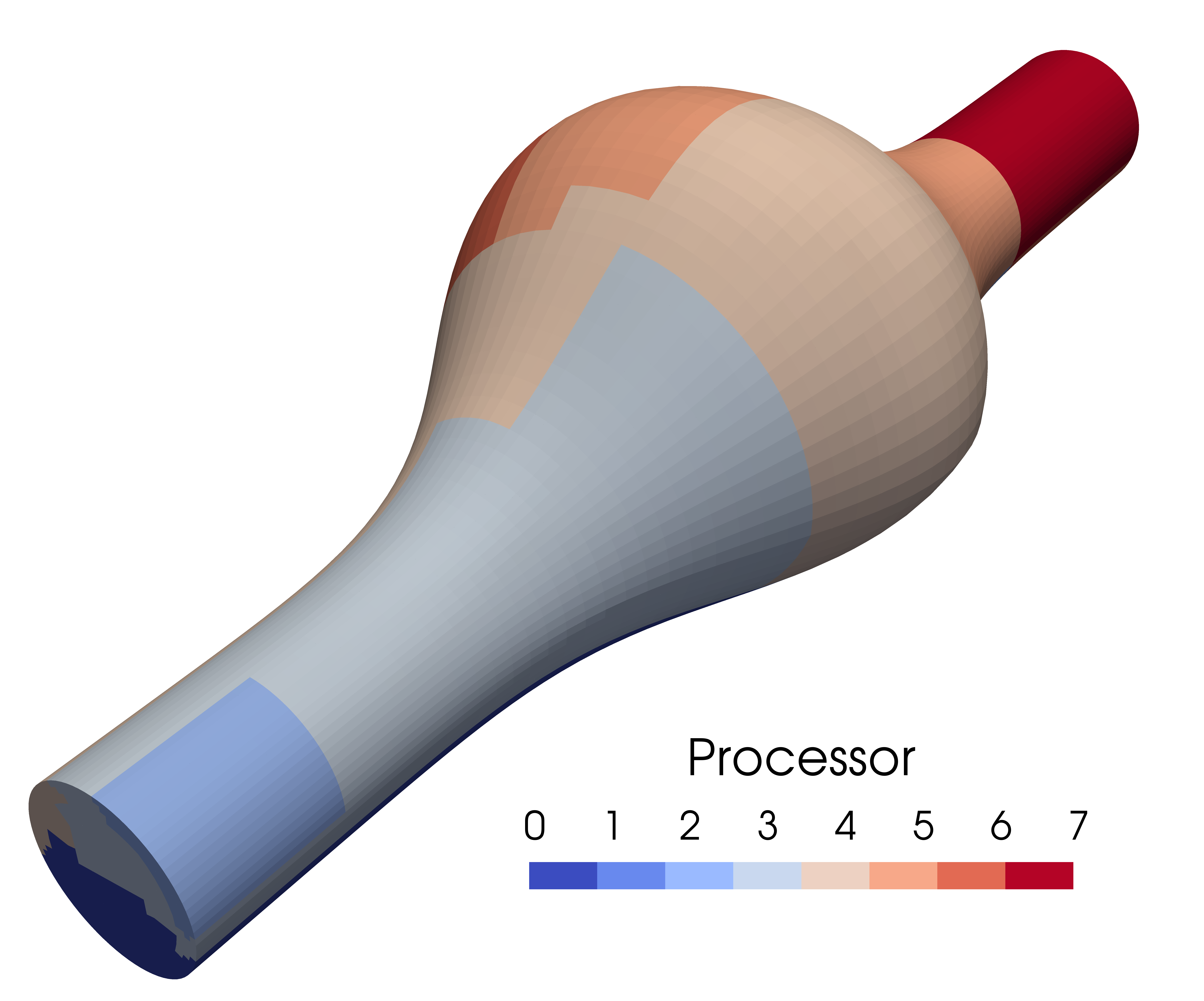
(a) Discretised AAA geometry.

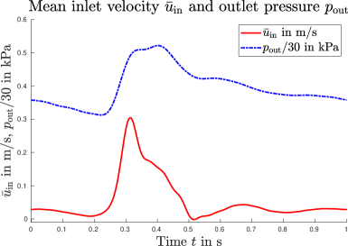
(b) In- and outlet data.

Figure 13: Realistic geometry distributed to 8 processors (left) and flow data (right) [157, 158, 159].

Regarding boundary conditions, we fix the nodes at the in- and outlet and consider a viscoelastic external tissue supporting the solid by enforcing

$$\text{\boldmath${P}$}{\hat{\text{\boldmath${n}$}}}_{s}=\text{\boldmath${t}$}_{s}=-k_{e}\text{\boldmath${d}$}_{s}-c_{e}\frac{\partial}{\partial t}\text{\boldmath${d}$}_{s}-p_{e}{\hat{\text{\boldmath${n}$}}}_{s}$$

via the boundary term on $\hat{\Gamma}_{{N,s}}$ with $k_{e}=10^{7}\leavevmode\nobreak\ \text{N/m}^{3}$, $c_{e}=10^{5}\leavevmode\nobreak\ \text{Ns/m}^{3}$ and $p_{e}=0\leavevmode\nobreak\ \text{N/m}^{2}$ chosen similar to [143, 145, 122]. The fluid inlet condition is computed from periodic mean inlet velocity $\bar{u}_{\mathrm{in}}$ as shown in Figure 13b, prescribing the normal inlet velocity component $u_{1}$ in terms of the distance from the circular inlet center $r$:

$$u_{1}=2\bar{u}_{\mathrm{in}}\left(1-\frac{r}{r_{\text{i}}}\right)\xi_{t}(t)\,,\text{ with}\quad\xi_{t}(t)=\begin{cases}\sin^{2}\left(\frac{\pi t}{0.4}\right)&\text{for}\ t\leq 0.2,\\ 1&\text{otherwise},\end{cases}$$

and a factor of 2 to match the volumetric flow rate computed from the mean velocity $\bar{u}_{\mathrm{in}}$ with a parabolic velocity profile. The outlet pressure is approximated via a three-element Windkessel model (see, e.g., [146, 147, 142, 122])

$$C\frac{\partial}{\partial t}p_{p}+\frac{p_{p}}{R_{d}}=Q(\text{\boldmath${u}$}_{f})\,,\quad p_{c}-p_{p}=R_{p}Q(\text{\boldmath${u}$}_{f})\,,$$

which represents the characteristics of the excluded downstream vasculature. Therein, the flow over the outlet is denoted as $Q(\text{\boldmath${u}$}_{f})$ and parameters for the capacitance $C=1.25\times 10^{-9}\leavevmode\nobreak\ \text{m${}^{4}$s${}^{2}$/kg}$ and the proximal and distal resistances are specified as $R_{p}=266.66\times 10^{5}\leavevmode\nobreak\ \text{kg/m${}^{4}$s}$ and $R_{d}=6.8\times 10^{8}\leavevmode\nobreak\ \text{kg/m${}^{4}$s}$, respectively. The outlet pressure is then weakly enforced through the standard traction boundary integral term, setting

$$\text{\boldmath${\sigma}$}_{f}\text{\boldmath${n}$}_{f}=-p_{c}\text{\boldmath${n}$}_{f}-\rho_{f}(\text{\boldmath${u}$}_{f}\cdot\text{\boldmath${n}$}_{f})_{-}\,,$$

also including backflow stabilisation according to [164], where $(\text{\boldmath${u}$}_{f}\cdot\text{\boldmath${n}$}_{f})_{-}=-\text{\boldmath${u}$}_{f}\cdot\text{\boldmath${n}$}_{f}$ for $\text{\boldmath${u}$}_{f}\cdot\text{\boldmath${n}$}_{f}\leq 0$ and $0$ otherwise. Moreover, Galerkin least-squares stabilisation [165] is added to the fluid momentum balance equation to counteract dominant convective terms.

Concerning material properties, we keep the physiological parameters as set in the pressure pulse benchmark, i.e., densities of $\rho_{f}=1060\leavevmode\nobreak\ \text{kg/m${}^{3}$}$ and $\rho_{s}=1200\leavevmode\nobreak\ \text{kg/m${}^{3}$}$, either a Newtonian fluid with viscosity $\mu_{f}=3.5\leavevmode\nobreak\ \text{mPa\leavevmode\nobreak\ s}$ or a Carreau fluid with $\eta_{0}=56\leavevmode\nobreak\ \text{mPa\leavevmode\nobreak\ s}$, $\eta_{\infty}=3.45\leavevmode\nobreak\ \text{mPa\leavevmode\nobreak\ s}$, $\lambda_{f}=3.313\leavevmode\nobreak\ \text{s}$ and $n=0.3568$, again, taken from [150]. For the solid, we consider a St. Venant–Kirchhoff solid or linear elasticity, both using a Young’s modulus $E_{s}=300\leavevmode\nobreak\ \text{kPa}$ and a Poisson’s ratio $\nu_{s}=0.3$ and compare with layered neo-Hookean models with $\nu_{s}=0.499$ and a shear rate of $\mu_{s,1}=62.1\leavevmode\nobreak\ \text{kPa}$ and $\mu_{s,2}=21.6\leavevmode\nobreak\ \text{kPa}$ for inner and outer layers, respectively. Fibers are included for the HGO model, setting $k_{1}=1.4\leavevmode\nobreak\ \text{kPa}$, $k_{2}=22.1$ and $\kappa_{c,1}=0.12$, $\alpha_{c,1}=27.47^{\circ}$ and $\kappa_{c,2}=0.25$, $\alpha_{c,2}=52.88^{\circ}$ for the media and adventitia layers of the aorta [151, 152]. The prestress present in the tissue in a geometry reconstructed from medical image data is not considered in this setup. However, we can interpret the present mesh as the zero-stress geometry being the result of the prestress strategy “deflating” the model as in [166, 167]. This slight discrepancy is simply ignored, since we do not investigate prestress effects.

Altogether, three pulses are considered, i.e., $t\in(0,3]$, using a uniform time step of $\Delta t=1\leavevmode\nobreak\ \text{ms}$ in the second-order accurate scheme, i.e., BDF-2 and linear extrapolation for linearisation. The WBZ$-\alpha$ and CH$-\alpha$ time integrators with $\rho_{\infty}=0$ are selected, since they were again found to be more robust when using the Windkessel model. Aitken’s relaxation is initiated with $\omega_{0}=0.001$, coupling the pressure Poisson (PPE) and solid momentum subproblems in the semi-implicit Dirichlet–Neumann (SIDN) approach until reaching $\epsilon_{abs}=10^{-6}$ or $\epsilon_{rel}=5\times 10^{-4}$, while a relative tolerance in the Newton solver (19) of $\epsilon_{N}=10^{-5}$ was selected conservatively.

Looking at solution snapshots at three distinct time instances at $t=2.2,2.4\text{ and }2.6\leavevmode\nobreak\ \text{s}$, we observe strong recirculations in the AAA, especially after the rapid drop of the inflow velocity. In Figure 14, selected streamlines indicate areas of recirculatory flow, leading to large gradients in the velocity fields and hence to a large shear rate, which ultimately results in strong gradients in the viscosity field. Further, the maximal and minimal viscosities observed at any point in time span almost the entire range from $\eta_{\infty}$ to $\eta_{0}$. The pressure in the lumen is spatially rather uniform, but rapidly changes in time due to the Windkessel model setting the pressure level, which dominates the deformation rather than the velocity acting on the vessel. Inspecting the time evolution of the displacement norm and fluid pressure at the apex point at $\hat{\text{\boldmath${x}$}}=(0.1,0.039,0)^{T}$ depicted in Figure 15, we see that the periodic state is not yet reached. This is due to the Windkessel model applied on the outflow boundary, which only gradually increases the pressure level in the AAA. Observing the displacement norm and fluid pressure only, effects of the more advanced solid constitutive models cannot be investigated, especially since the displacement remains rather small. The parameter choice for the tissue, however, leads to a difference easily observable with the naked eye.

Regarding the difference when applying Newtonian or Carreau rheological models, Figure 15 is not sufficient, since the relevant quantities are neither the displacement nor the pressure, but rather the time averaged shear rate and shear stress. After defining the time average $\bar{f}(\text{\boldmath${x}$})$ of a function $f(\text{\boldmath${x}$},t)$ over a period $T_{p}$ by

$$\bar{f}=\frac{1}{T_{p}}\int_{iT_{p}}^{(i+1)T_{p}}f(\mathcal{A}_{t}(\hat{\text{\boldmath${x}$}},t),t)\text{d}t\,,$$

calculate $\bar{\dot{\gamma}}$ setting $i=T_{p}=1$, while the shear stress is computed following John et al. [168]:

$${\tau} =\text{\boldmath${\sigma}$}_{f}\text{\boldmath${n}$}_{f}-\left[(\text{\boldmath${\sigma}$}_{f}\text{\boldmath${n}$}_{f})\cdot\text{\boldmath${n}$}_{f}\right]\text{\boldmath${n}$}_{f}=\left(2\mu_{f}\nabla^{S}\text{\boldmath${u}$}_{f}\right)\text{\boldmath${n}$}_{f}-\left\{\left[\left(2\mu_{f}\nabla^{S}\text{\boldmath${u}$}_{f}\right)\text{\boldmath${n}$}_{f}\right]\cdot\text{\boldmath${n}$}_{f}\right\}\text{\boldmath${n}$}_{f}\,.$$

Inspecting these time averaged quantities in the third cycle, as shown in Figure 16, a striking difference is observed as expected. Nonetheless, within this work we focus on the FSI solver rather than the phenomenological influence of different model decisions, but still want to demonstrate the versatility of the framework.

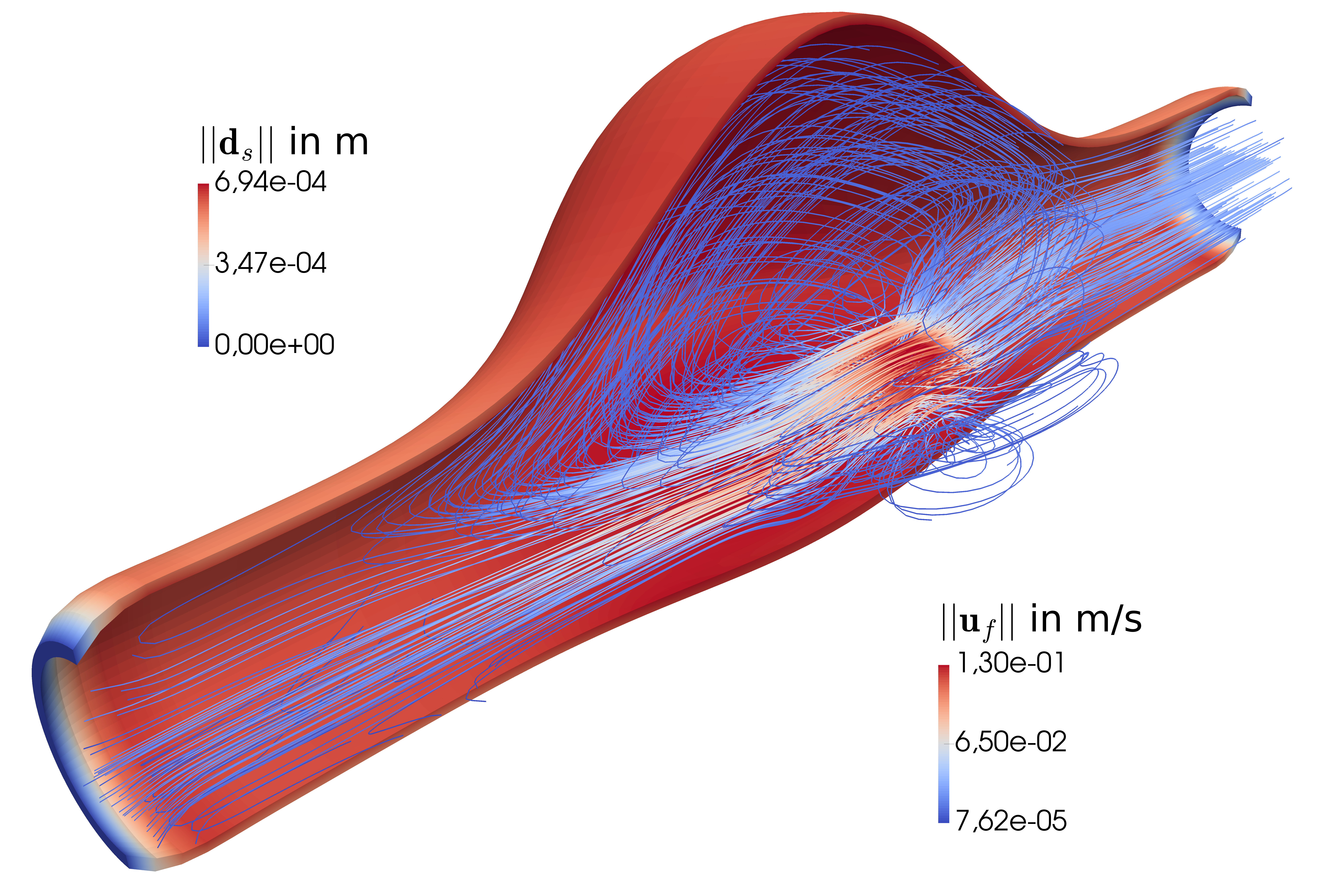
(a) $\text{\boldmath${d}$}_{s}$ and $\text{\boldmath${u}$}_{f}$ at $t=2.2\leavevmode\nobreak\ \text{s}$.

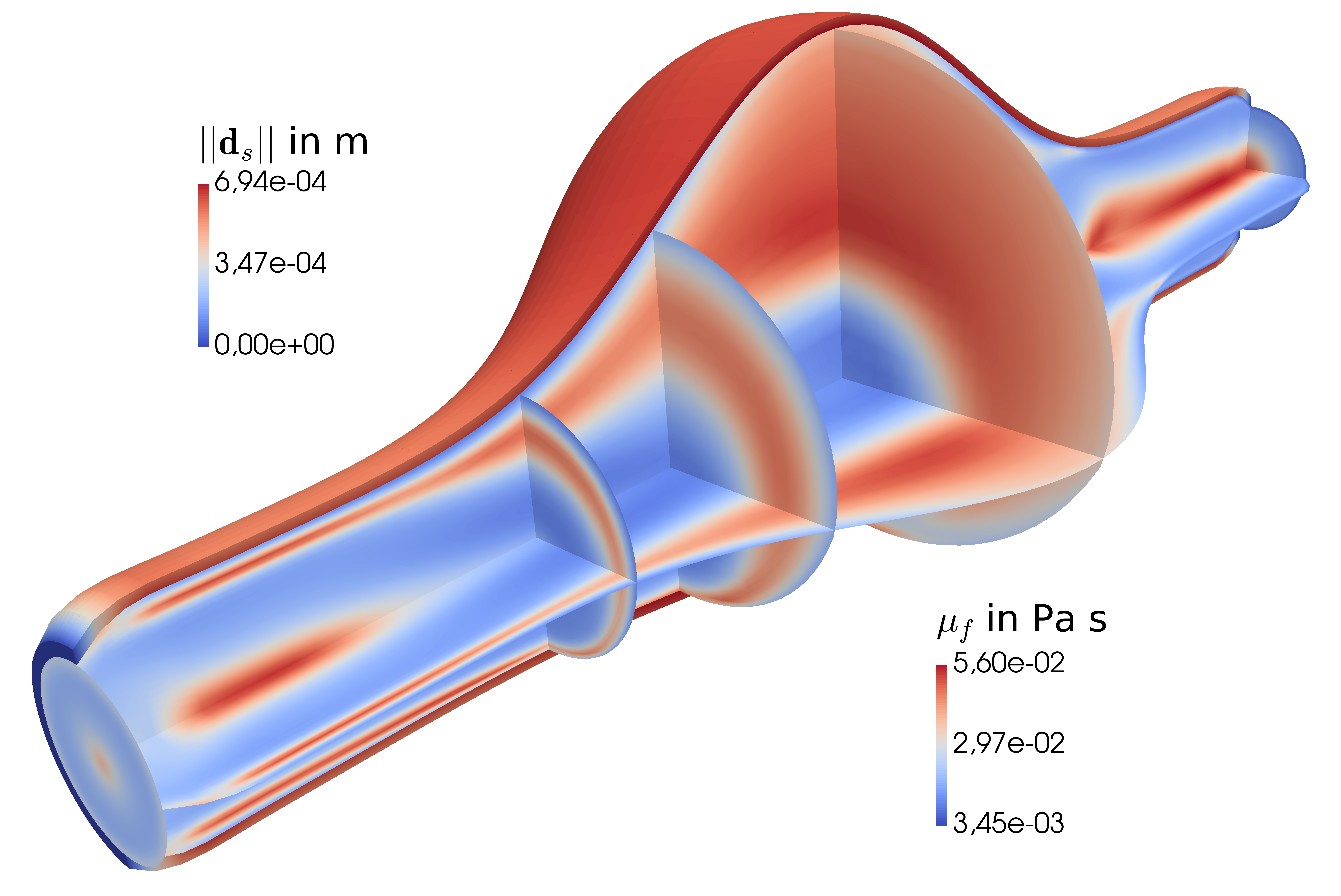
(b) $\text{\boldmath${d}$}_{s}$ and $\mu_{f}$ at $t=2.2\leavevmode\nobreak\ \text{s}$.

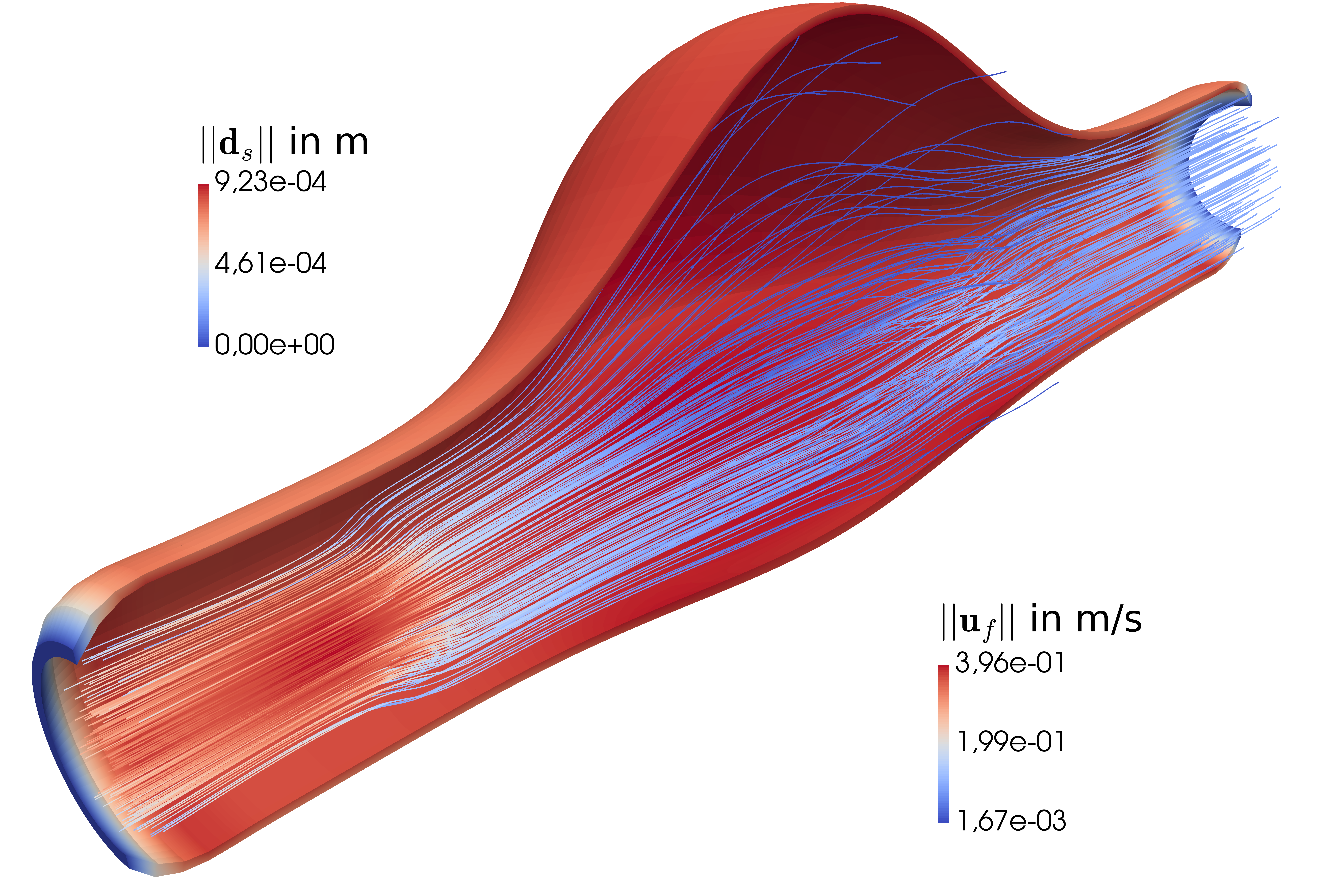
(c) $\text{\boldmath${d}$}_{s}$ and $\text{\boldmath${u}$}_{f}$ at $t=2.4\leavevmode\nobreak\ \text{s}$.

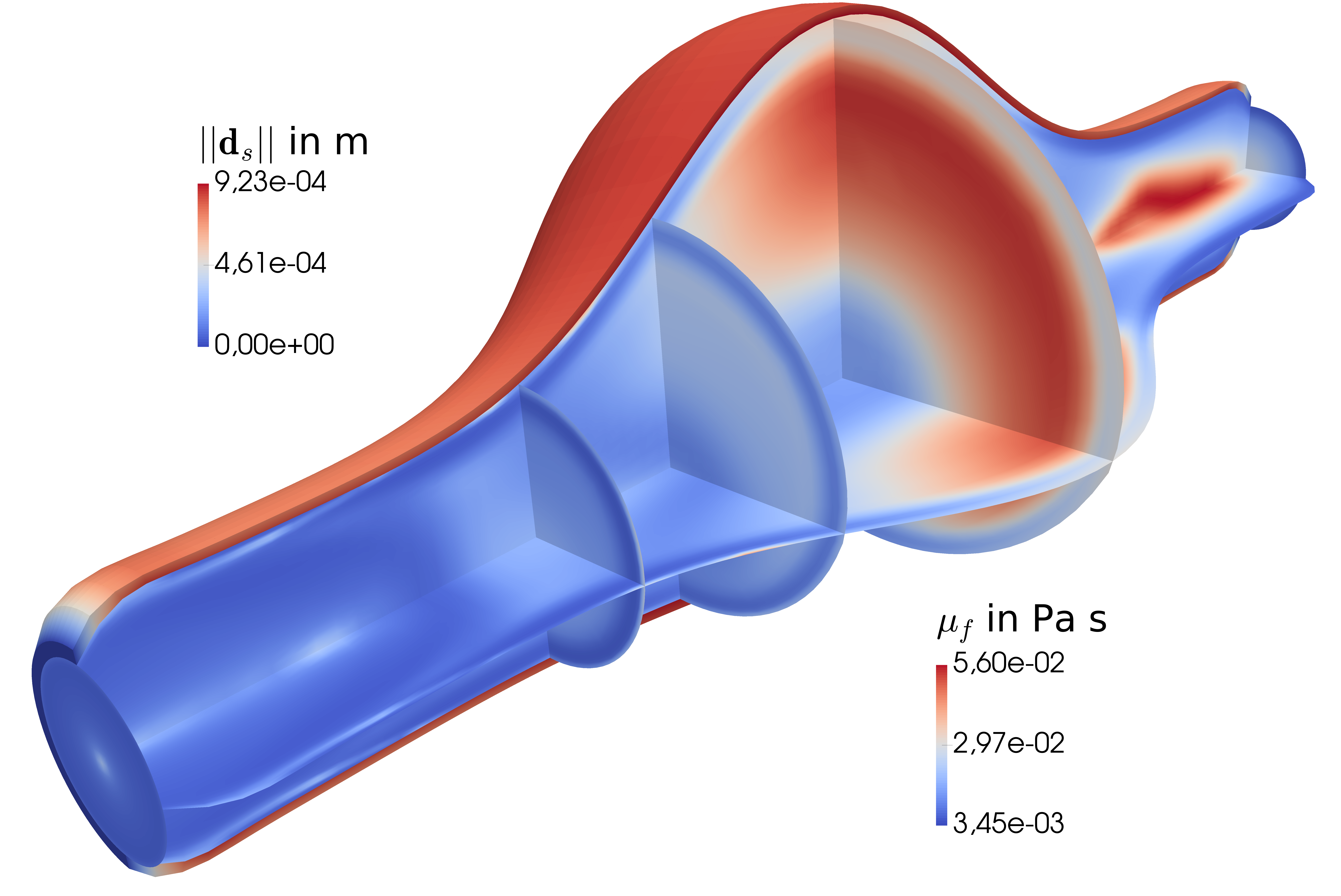
(d) $\text{\boldmath${d}$}_{s}$ and $\mu_{f}$ at $t=2.4\leavevmode\nobreak\ \text{s}$.

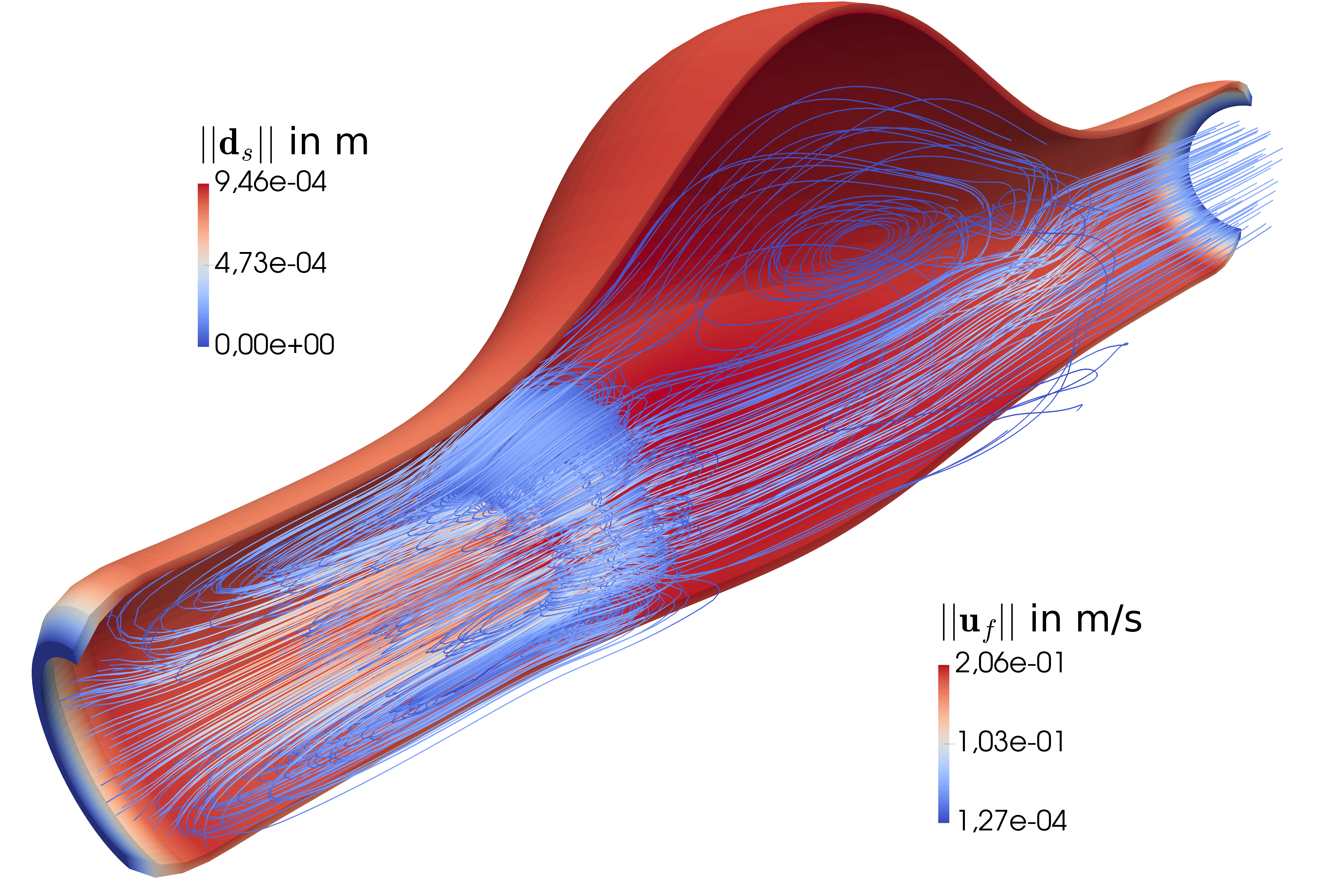
(e) $\text{\boldmath${d}$}_{s}$ and $\text{\boldmath${u}$}_{f}$ at $t=2.6\leavevmode\nobreak\ \text{s}$.

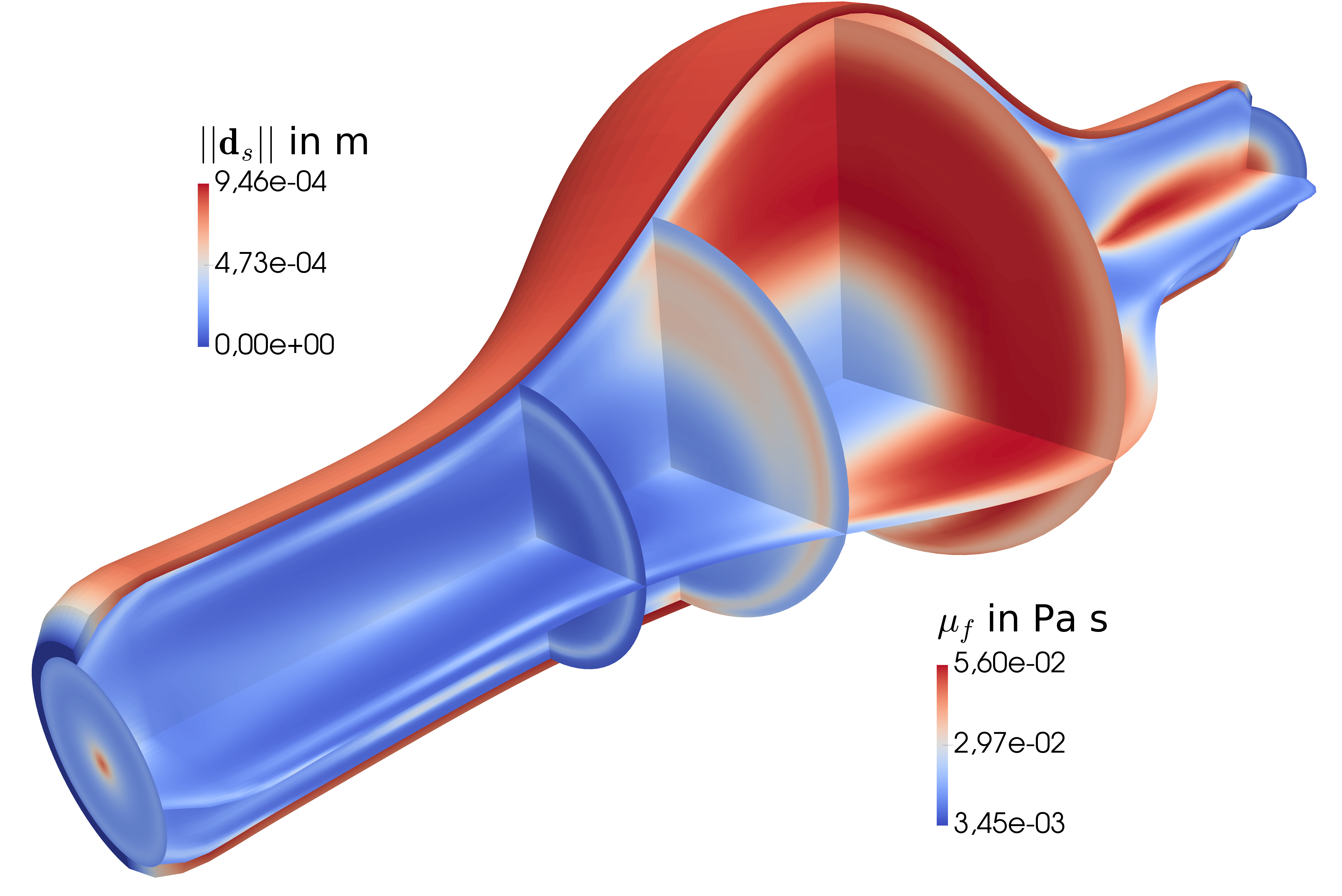
(f) $\text{\boldmath${d}$}_{s}$ and $\mu_{f}$ at $t=2.6\leavevmode\nobreak\ \text{s}$.

Figure 14: Snapshots at time $t=2.2,2.4,2.6\leavevmode\nobreak\ \text{s}$ Carreau fluid flowing through the abdominal aortic aneurysm of HGO material (deformation scaled by $5$): Solid displacement $\text{\boldmath${d}$}_{s}$ and selected streamlines of the fluid velocity $\text{\boldmath${u}$}_{f}$ (left) or viscosity $\mu_{f}$ in selected slices (right).

(a) $||\text{\boldmath${d}$}_{s}||$ in the apex point.

(b) $||p_{f}||$ in the apex point.

Figure 15: Solid displacement and fluid pressure in the apex point using linear elasticity (E), neo-Hookean (NH) or Holzapfel–Gasser–Ogden (HGO) material models for the solid phase and Newtonian (N) or Carreau (C) fluids. The periodic state is not yet reached due to the Windkessel model. Effects of nonlinearities are small in the observed quantities.

Having thoroughly inspected the solution itself, let us now turn our attention to the numerical aspects of this test case. Motivated by the previous example, the semi-implicit Dirichlet–Neumann (SIDN) coupling scheme is considered. Throughout the entire simulation time, less than 30 steps coupling solid momentum balance and PPE are needed, as shown in Figure 17. Only a slight dependence on the inflow profile and pressure level in the geometry are observed. Interestingly, accumulated FSI iteration counts show that NH and HGO models lead to fewer FSI iterations, which is most likely triggered by higher pressure levels due to a stiffer material response caused by the selected (higher) Young’s modulus. For comparison, the implicit Dirichlet–Neumann (IDN) scheme and a scheme treating the mesh motion explicitly, leading to a geometry explicit (GEDN) approach are also included in Figure 17b, showing a decrease of up to 31% in FSI coupling steps needed when using the semi-implicit variant.

(a) $\bar{\text{\boldmath${\tau}$}}$ on the fluid–structure interface $\Sigma^{t}$.

(b) $\bar{\dot{\gamma}}$ in cut fluid domain $\Omega_{f}^{t}$.

Figure 16: Time averaged quantities in anterior-posterior view, inlet on the right: the symmetric solutions show vast differences using Newtonian (top row) and Carreau (bottom row) models.

(a) Coupling steps per time step.

(b) Accumulated coupling steps.

Figure 17: Coupling steps needed using the semi-implicit (SIDN), implicit (IDN) or geometry explicit (GEDN) Dirichlet–Neumann schemes: iterations per time step (left) and accumulated (right) comparing linear elasticity (E), neo-Hookean (NH) or Holzapfel–Gasser–Ogden (HGO) material models for the solid phase and Newtonian (N) or Carreau (C) fluids.

Regarding the iteration counts in the subproblems, consider first systems solved only once per time step. Solving the linear system corresponding to the fluid momentum balance equations needs an almost constant number of 3 iterations to reach a relative error of $\leq 10^{-8}$ applying the AMG-preconditioned FGMRES method using a Chebyshev smoother due to small enough time steps. The iteration counts over time are depicted in Figure 18 together with the iteration counts needed so solve the mesh motion equation with an AMG-preconditioned CG solver. The mass matrix corresponding to the viscosity projection step is lumped and therefore easily inverted, simply scaling the assembled right-hand side by a vector representing the diagonal. The iteration counts for the Leray projection step stay nicely bounded around $\approx 35$. For brevity, we do not show a corresponding plot, since it behaves similar to the PPE and is only computed once per time step – in fact, one can combine PPE and Leray projection steps of the past velocities when using divergence damping, solving only one Poisson problem for a combined variable. This detail does barely pay off using the SIDN scheme, which is why we refer to [110] for further details.

(a) FGMRES steps needed for linear solver convergence in the fluid momentum balance.

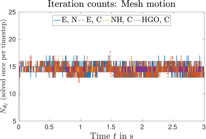
(b) CG steps needed for linear solver convergence in the mesh motion equation.

Figure 18: Iteration counts in the fluid momentum balance (left) and mesh motion (right) solvers using linear elasticity (E), neo-Hookean (NH) or Holzapfel–Gasser–Ogden (HGO) material models for the solid phase, Newtonian (N) or Carreau (C) fluids and the SIDN scheme.

For the overall performance, the steps within the semi-implicit coupling loop, namely the PPE and solid momentum balance solves are dominant in terms of computational effort. Thus, the good performance of the linear solvers as depicted in Figure 19 is crucial. We observe little dependence on the fluid velocity and pressure level, given the relatively small time step size. Additionally, nonlinear convergence in the Newton solver is reached in any time step within 3 iterations, which is also a result of the small time step size and the quadratic extrapolation used as an initial guess. Comparing the constitutive models, the linear solvers show equal behaviour independent of the fluid model employed. The solid model, however, heavily influences the iteration count in the linear system solve, resulting from the more complex terms and matrices when considering NH or HGO models.

(a) CG steps needed for linear solver convergence in the PPE.

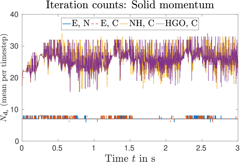
(b) FGMRES steps needed for linear solver convergence in the solid momentum balance.

Figure 19: Iteration counts in the PPE (left) and solid momentum balance (right) solvers using linear elasticity (E), neo-Hookean (NH) or Holzapfel–Gasser–Ogden (HGO) material models for the solid phase, Newtonian (N) or Carreau (C) fluids and the SIDN scheme.

Summing up, the solutions of the linear systems corresponding to each of the subproblems are obtained within a satisfactory number of iterations and show low iteration counts given the relevant parameter ranges including realistic Reynold’s numbers and tissue stiffness. As a last note on the computational performance of the implementation, compare the absolute and relative time spent per time step using different constitutive models. As can be seen from Table 3, the number of FSI coupling steps needed for convergence are slightly higher for stiffer material parameters, while the viscosity projection step is negligible in terms of computational effort. The solid constitutive models, however, do have a strong influence on the time spent per time step. This additional effort is caused by both the increased complexity of element integration and $\approx 2.5\times$ more iterations in the linear system solve (see also Figure 19). The SIDN variant outperforms the GEDN and IDN schemes being at least twice as fast overall, needing less FSI iterations and less time per coupling step. Interestingly, the number of coupling steps increases when using the GEDN scheme, but individual steps and the overall time interval are completed faster compared to the IDN scheme, since the mesh motion equation is only solved once per time step.

	computing time	FSI steps	time/FSI step
E, N (SIDN)	$5.53\times 10^{5}\leavevmode\nobreak\ \text{s}$ (100.0%)	21046 (121.0%)	$26.3\leavevmode\nobreak\ \text{s}$ (100.0%)
E, C (SIDN)	$5.57\times 10^{5}\leavevmode\nobreak\ \text{s}$ (100.1%)	21118 (121.4%)	$26.4\leavevmode\nobreak\ \text{s}$ (100.4%)
NH, C (SIDN)	$9.22\times 10^{5}\leavevmode\nobreak\ \text{s}$ (166.7%)	17395 (100.0%)	$53.0\leavevmode\nobreak\ \text{s}$ (201.5%)
HGO, C (SIDN)	$1.09\times 10^{6}\leavevmode\nobreak\ \text{s}$ (196.4%)	17846 (102.6%)	$56.5\leavevmode\nobreak\ \text{s}$ (214.8%)
E, N (GEDN)	$1.07\times 10^{6}\leavevmode\nobreak\ \text{s}$ (193.5%)	27532 (158.3%)	$38.9\leavevmode\nobreak\ \text{s}$ (147.9%)
E, N (IDN)	$1.41\times 10^{6}\leavevmode\nobreak\ \text{s}$ (255.0%)	27045 (155.5%)	$52.3\leavevmode\nobreak\ \text{s}$ (198.9%)

Table 3: Absolute (relative) computing times using linear elasticity (E), neo-Hookean (NH) or Holzapfel–Gasser–Ogden (HGO) material models for the solid phase, Newtonian (N) or Carreau (C) fluids and the semi-implicit (SIDN), implicit (IDN) or geometry explicit (GEDN) Dirichlet–Neumann coupling schemes.

	$\text{\boldmath${d}$}_{f}$	$\text{\boldmath${u}$}_{f}$	$\psi$	$\zeta$	$p_{f}$	$\text{\boldmath${d}$}_{s}$
E, N	6.0	8.0	4.8	2.6	(6.4+4.2+19.7)	(20.3+4.9+16.2)
E, C	5.9	8.0	4.9	2.6	(6.3+4.2+19.5)	(20.2+4.9+16.2)
NH, C	2.3	2.2	3.3	0.8	(1.6+2.6+14.5)	(29.5+5.1+35.7)
HGO, C	1.6	1.7	2.2	0.6	(1.3+1.9+10.4)	(47.6+3.7+26.9)

Table 4: Relative computing times of relevant steps, indicated by the unknown solved for in the SIDN scheme: in %, split into (assembly+AMG setup+linear solve) for PPE and solid momentum balance using linear elasticity (E), neo-Hookean (NH) or Holzapfel–Gasser–Ogden (HGO) material models for the solid phase and Newtonian (N) or Carreau (C) fluids.

Timings for the computationally relevant steps within the SIDN coupling scheme are further listed in Table 4, where we notice the increased (relative) time spent in those steps. Also, this demonstrates how little time is spent on the semi-implicit steps, being the mesh motion equation ($\text{\boldmath${d}$}_{f}$), fluid momentum balance ($\text{\boldmath${u}$}_{f}$), Leray projection ($\psi$) and viscosity projection, the last one of which is not even listed since the time spent is less than $0.5\%$. The pressure boundary projection ($\zeta$) is performed in each coupling step, but still does not lead to a major computational load. Solving the PPE ($p_{f}$) and solid momentum balance ($\text{\boldmath${d}$}_{s}$) has the largest influence on the overall time spent in the SIDN scheme, where one may further optimise element integration routines and linear solvers. Nonetheless, iteration counts are nicely bounded, indicating good performance of the chosen setup. Parallel scalability of the overall algorithm is not investigated at this point, but aspect of future investigations.

5 Concluding remarks

Within this work, we presented a family of coupling schemes involving incompressible viscous flows interacting with three-dimensional solids. The standard Navier–Stokes equations were solved by decoupling velocity and pressure via an equivalent time-splitting or split-step scheme in arbitrary Lagrangian-Eulerian formulation, based on a pressure Poisson equation with consistent boundary conditions. Consequently, substantial parts of the algorithm can be treated semi-implicitly in an added-mass-stable way without degrading accuracy. The mesh motion equation, fluid momentum balance equation, Leray projection (included for improved mass conservation) and viscosity projection are only solved once per time step. Generalised Newtonian rheological laws are exchanged effortlessly, while also allowing for equal order, $C^{0}$-continuous interpolation with Lagrangian finite elements. Moreover, we considered a general setup including various constitutive models applied for the solid, demonstrating the flexibility of the framework and robustness of the coupling algorithm. The accuracy of the scheme is assessed comparing to analytical solutions in space, applying $Q_{2}/Q_{1}$ and $Q_{1}/Q_{1}$ finite element pairs, and in time, combining BDF-2 with generalised-$\alpha$ time integration schemes. The framework is then further tested in a benchmark example in the context of arterial blood flow and an idealised abdominal aortic aneurysm, highlighting its great performance even with black-box solvers and preconditioners.

Future and ongoing work is centered around scalability tests and algorithmic optimisation to further reduce runtimes. From a modelling perspective, other constitutive equations and mixed/hybrid formulations for the solid phase will be included, harnessing the partitioned design. Moreover, we are testing semi-implicit coupling to thrombus formation models, which is a central element in various cardiovascular conditions.

Competing interests

The authors declare that they have no known competing financial interests or personal relationships that could have appeared to influence the work reported in this paper.

Appendix

Proof of equivalence of systems (30)–(35) and (22)–(27) for sufficiently regular $p_{f},\text{\boldmath${u}$}_{f},\text{\boldmath${g}$}_{f},\text{\boldmath${t}$}_{f},\text{\boldmath${h}$}_{f}$ (Theorem 2.1).

Proof.

We start by showing first that (22)–(27) imply (30)–(35), where the stress term in the momentum balance equation (22) is simply rewritten according to (28) to obtain (30). The Dirichlet conditions on the pressure (33) is obtained by the traction boundary condition (26) and ${\text{\boldmath${n}$}}_{f}$ first

$${\text{\boldmath${n}$}}_{f}\cdot\left(\text{\boldmath${\sigma}$}_{f}{\text{\boldmath${n}$}}_{f}-\text{\boldmath${t}$}_{f}\right)=\text{\boldmath${0}$}\quad\Leftrightarrow\quad{\text{\boldmath${n}$}}_{f}\cdot\left(2\mu_{f}\nabla^{S}\text{\boldmath${u}$}_{f}{\text{\boldmath${n}$}}_{f}\right)-{\text{\boldmath${n}$}}_{f}\cdot\text{\boldmath${t}$}_{f} ={\text{\boldmath${n}$}}_{f}\cdot\left(p_{f}\text{\boldmath${I}$}{\text{\boldmath${n}$}}_{f}\right)=p_{f}$$

and then subtracting $\mu_{f}\nabla\cdot\text{\boldmath${u}$}_{f}$ from the left hand side, which is admissible due to $\nabla\cdot\text{\boldmath${u}$}_{f}=0$. Analogously, a boundary condition based on the Robin condition (27) is derived. The Neumann condition on the pressure (35) results from the momentum balance equation (22) and ${\text{\boldmath${n}$}}_{f}$ and using

$$-\nabla\cdot\text{\boldmath${\sigma}$}_{f} =-\nabla\cdot\left\{-\left(p_{f}\text{\boldmath${I}$}\right)+\mu_{f}\left[\nabla\text{\boldmath${u}$}_{f}+\left(\nabla\text{\boldmath${u}$}_{f}\right)^{T}\right]\right\}$$

$$=\nabla p_{f}-\mu_{f}\nabla\left(\nabla\cdot\text{\boldmath${u}$}_{f}\right)-\mu_{f}\Delta\text{\boldmath${u}$}_{f}-2\nabla^{S}\text{\boldmath${u}$}_{f}\nabla\mu_{f}$$

$$=\nabla p_{f}-\mu_{f}\Delta\text{\boldmath${u}$}_{f}-2\nabla^{S}\text{\boldmath${u}$}_{f}\nabla\mu_{f}$$ (68)

for $\nabla\cdot\text{\boldmath${u}$}_{f}=0$ together with

$$\Delta\text{\boldmath${u}$}_{f}\equiv\nabla\left(\nabla\cdot\text{\boldmath${u}$}_{f}\right)-\nabla\times\left(\nabla\times\text{\boldmath${u}$}_{f}\right)=-\nabla\times\left(\nabla\times\text{\boldmath${u}$}_{f}\right)\,,$$ (69)

which, restricted to ${\Gamma}_{{D,f}}^{t}$, directly gives (35). Similarly, taking (minus) the divergence of the balance of linear momentum, we get

$${0} =-\rho_{f}\nabla\cdot\left[\left.\frac{\partial}{\partial t}\text{\boldmath${u}$}_{f}\right|_{\mathcal{A}_{t}}+\nabla\text{\boldmath${u}$}_{f}\left(\text{\boldmath${u}$}_{f}-\text{\boldmath${u}$}_{m}\right)\right]+\nabla\cdot\left(\nabla\cdot\text{\boldmath${\sigma}$}_{f}\right)$$

$$=\rho_{f}\left.\frac{\partial}{\partial t}\left(\nabla\cdot\text{\boldmath${u}$}_{f}\right)\right|_{\mathcal{A}_{t}}-\nabla\cdot\left[\rho_{f}\nabla\text{\boldmath${u}$}_{f}\left(\text{\boldmath${u}$}_{f}-\text{\boldmath${u}$}_{m}\right)-2\nabla^{S}\text{\boldmath${u}$}_{f}\nabla\mu_{f}\right]+\nabla\cdot\left(\mu_{f}\Delta\text{\boldmath${u}$}_{f}\right)-\Delta p_{f}$$

$$=-\nabla\cdot\left[\rho_{f}\nabla\text{\boldmath${u}$}_{f}\left(\text{\boldmath${u}$}_{f}-\text{\boldmath${u}$}_{m}\right)-2\nabla^{S}\text{\boldmath${u}$}_{f}\nabla\mu_{f}\right]+\nabla\cdot\left(\mu_{f}\Delta\text{\boldmath${u}$}_{f}\right)-\Delta p_{f}\,,$$

but with (69) we can rewrite

$$\nabla\cdot\left(\mu_{f}\Delta\text{\boldmath${u}$}_{f}\right)=-\nabla\cdot\left[\mu_{f}\nabla\times\left(\nabla\times\text{\boldmath${u}$}_{f}\right)\right]=-\left[\nabla\times\left(\nabla\times\text{\boldmath${u}$}_{f}\right)\right]\cdot\nabla\mu_{f}\,,$$ (70)

which then finally gives Equation (31). The additional Equation (32) is simply the continuity equation at $t=0$, thus completing the first part. To finish the proof of equivalence, we start from the other direction, i.e., show that (30)–(35) imply (22)–(27) by first taking minus the divergence of (30) and adding it to (31), which gives

$$-\rho_{f}\nabla\cdot\left(\left.\frac{\partial}{\partial t}\text{\boldmath${u}$}_{f}\right|_{\mathcal{A}_{t}}\right)+\nabla\cdot\left[\nabla\cdot\left(2\mu_{f}\nabla^{S}\text{\boldmath${u}$}_{f}\right)\right]-\nabla\cdot\left[2\nabla^{S}\text{\boldmath${u}$}_{f}\nabla\mu_{f}\right]+\left[\nabla\times\left(\nabla\times\text{\boldmath${u}$}_{f}\right)\right]\cdot\nabla\mu_{f}=0\,,$$

where we can further use relations similar to (69) and  (68) to get

$$-\rho_{f}\nabla\cdot\left(\left.\frac{\partial}{\partial t}\text{\boldmath${u}$}_{f}\right|_{\mathcal{A}_{t}}\right)+\nabla\cdot\left[\mu_{f}\nabla(\nabla\cdot\text{\boldmath${u}$}_{f})+\mu_{f}\Delta\text{\boldmath${u}$}_{f}\right]+\left[\nabla(\nabla\cdot\text{\boldmath${u}$}_{f})-\Delta\text{\boldmath${u}$}_{f}\right]\cdot\nabla\mu_{f}=0\,,$$

where we use (69) and (70), but without inserting $\nabla\cdot\text{\boldmath${u}$}_{f}=0$, to finally arrive at

$$\left.\frac{\partial}{\partial t}(\nabla\cdot\text{\boldmath${u}$}_{f})\right|_{\mathcal{A}_{t}}-\nabla\cdot\left[2\frac{\mu_{f}}{\rho_{f}}\nabla(\nabla\cdot\text{\boldmath${u}$}_{f})\right]=0\,,$$ (71)

being a heat equation in the new variable $\Phi:=\nabla\cdot\text{\boldmath${u}$}_{f}$ in ALE form. Neumann conditions for (71) are obtained by  (30) and $\text{\boldmath${n}$}_{f}$ and adding the result to (35), which gives

$$\text{\boldmath${n}$}_{f}\cdot\left\{-\nabla\cdot(2\mu_{f}\nabla^{S}\text{\boldmath${u}$}_{f})-\mu_{f}\left[\nabla\times(\nabla\times\text{\boldmath${u}$}_{f})\right]+2\nabla^{S}\text{\boldmath${u}$}_{f}\right\}=0\,.$$

Further using once again  (69) and  (68), we end up with

$$0=\text{\boldmath${n}$}_{f}\cdot\left[-2\mu_{f}\nabla(\nabla\cdot\text{\boldmath${u}$}_{f})\right]\quad\therefore\quad\text{\boldmath${n}$}_{f}\cdot\nabla\Phi=0\quad\text{on }{\Gamma}_{{D,f}}^{t}\,.$$ (72)

Dirichlet conditions for (71) are constructed from (33) and (34), which after inserting the definition of $\text{\boldmath${t}$}_{f}$ and $\text{\boldmath${h}$}_{f}$, respectively, directly result in

$$-\mu_{f}\nabla\cdot\text{\boldmath${u}$}_{f}=0\quad\therefore\quad\Phi=0\quad\text{on }\partial\Omega_{f}^{t}\setminus{\Gamma}_{{D,f}}^{t}\,.$$ (73)

Given these zero Neumann and Dirichlet conditions for $\Phi$, and assuming the geometric conservation law is fulfilled, i.e., a constant quantity is preserved on the moving grid (cf. [169, 170, 171, 172]) we obtain $\Phi\equiv 0$ as the only admissible solution to (71)–(73). Consequently, the modified system also inherently enforces incompressibility and we conclude the proof by quickly noting that equivalence of (30) and (22) is easily shown using (68) again. ∎

References

- Machairas et al. [2018] T. Machairas, A. Kontogiannis, A. Karakalas, A. Solomou, V. Riziotis, and D. Saravanos. Robust fluid-structure interaction analysis of an adaptive airfoil using shape memory alloy actuators. Smart Mater Struct, 27(10):105035, 2018.
- Bazilevs et al. [2011] Y. Bazilevs, M.-C. Hsu, I. Akkerman, S. Wright, K. Takizawa, B. Henicke, T. Spielman, and T.E. Tezduyar. 3D simulation of wind turbine rotors at full scale. Part I: Geometry modeling and aerodynamics. Int J Numer Methods Fluids, 65(1-3):207–235, 2011.
- Helgedagsrud et al. [2019] T.A. Helgedagsrud, Y. Bazilevs, K.M. Mathisen, and O.A. Øiseth. ALE-VMS methods for wind-resistant design of long-span bridges. J Wind Eng Ind Aerodyn, 191:143–153, 2019.
- Shiels et al. [2001] D. Shiels, A. Leonard, and A. Roshko. Flow-induced vibration of a circular cylinder at limiting structural parameters. J Fluids Struct, 15(1):3–21, 2001.
- Bearman [2011] P.W. Bearman. Circular cylinder wakes and vortex-induced vibrations. J Fluids Struct, 27(5-6):648–658, 2011.
- Chu et al. [2021] Y.J. Chu, P.B. Ganesan, and M.A. Ali. Fluid–structure interaction simulation on flight performance of a dragonfly wing under different pterostigma weights. J Mech, 37:216–229, 2021. ISSN 1811-8216.
- Bazilevs et al. [2006] Y. Bazilevs, V.M. Calo, Y. Zhang, and T.J.R. Hughes. Isogeometric Fluid–structure Interaction Analysis with Applications to Arterial Blood Flow. Comput Mech, 38(4-5):310–322, 2006.
- Crosetto et al. [2011a] P. Crosetto, S. Deparis, G. Fourestey, and A. Quarteroni. Parallel Algorithms for Fluid-Structure Interaction Problems in Haemodynamics. SIAM J Sci Comput, 33(4):1598–1622, 2011a.
- Crosetto et al. [2011b] P. Crosetto, P. Reymond, S. Deparis, D. Kontaxakis, N. Stergiopulos, and A. Quarteroni. Fluid–structure interaction simulation of aortic blood flow. Comput Fluids, 43(1):46–57, 2011b.
- Küttler et al. [2010] U. Küttler, M. Gee, C. Förster, A. Comerford, and W.A. Wall. Coupling strategies for biomedical fluid-structure interaction problems. Int J Numer Method Biomed Eng, 2010.
- Torii et al. [2006] R. Torii, M. Oshima, T. Kobayashi, K. Takagi, and T.E. Tezduyar. Computer modeling of cardiovascular fluid–structure interactions with the deforming-spatial-domain/stabilized space–time formulation. Comput Methods Appl Mech Eng, 195(13-16):1885–1895, 2006.
- Schussnig et al. [2021a] R. Schussnig, M. Rolf-Pissarczyk, G. Holzapfel, and T.-P. Fries. Fluid‐Structure Interaction Simulations of Aortic Dissection. PAMM, 20(1), 2021a.
- Thomson et al. [2005] S.L. Thomson, L. Mongeau, and S.H. Frankel. Aerodynamic transfer of energy to the vocal folds. J Acoust Soc Am, 118(3):1689–1700, 2005.
- Wall and Rabczuk [2008] W.A. Wall and T. Rabczuk. Fluid–structure interaction in lower airways of CT-based lung geometries. Int J Numer Methods Fluids, 57(5):653–675, 2008.
- Heil [2004] M. Heil. An efficient solver for the fully coupled solution of large-displacement fluid–structure interaction problems. Comput Methods Appl Mech Eng, 193(1-2):1–23, 2004.
- Hughes et al. [1981] T.J.R. Hughes, W.K. Liu, and T.K. Zimmermann. Lagrangian-Eulerian finite element formulation for incompressible viscous flows. Comput Methods Appl Mech Eng, 29(3):329–349, 1981.
- Le Tallec and Mouro [2001] P. Le Tallec and J. Mouro. Fluid structure interaction with large structural displacements. Comput Methods Appl Mech Eng, 190(24-25):3039–3067, 2001.
- Leuprecht et al. [2002] A. Leuprecht, K. Perktold, M. Prosi, T. Berk, W. Trubel, and H. Schima. Numerical study of hemodynamics and wall mechanics in distal end-to-side anastomoses of bypass grafts. J Biomech, 35(2):225–236, 2002.
- Forti et al. [2017] D. Forti, M. Bukac, A. Quaini, S. Canic, and S. Deparis. A Monolithic Approach to Fluid–Composite Structure Interaction. J Sci Comput, 72(1):396–421, 2017.
- Quaini and Quarteroni [2007] A. Quaini and A. Quarteroni. A semi-implicit approach for fluid-structure interaction based on an algebraic fractional step method. Math Models Methods Appl Sci, 17(06):957–983, 2007.
- Quarteroni et al. [2000] A. Quarteroni, M. Tuveri, and A. Veneziani. Computational vascular fluid dynamics: problems, models and methods. Comput Vis Sci, 2(4):163–197, 2000.
- Donea et al. [1982] J. Donea, S. Giuliani, and J.P. Halleux. An arbitrary lagrangian-eulerian finite element method for transient dynamic fluid-structure interactions. Comput Methods Appl Mech Eng, 33(1-3):689–723, 1982.
- Fauci and Dillon [2006] L.J. Fauci and R. Dillon. Biofluidmechanics of reproduction. Annu Rev Fluid Mech, 38(1):371–394, 2006.
- Fogelson [2004] A.L. Fogelson. Platelet-wall interactions in continuum models of platelet thrombosis: formulation and numerical solution. Math Med Biol, 21(4):293–334, 2004.
- Griffith [2012] B.E. Griffith. Immersed boundary model of aortic heart valve dynamics with physiological driving and loading conditions. Int J Numer Method Biomed Eng, 28(3):317–345, 2012.
- Griffith et al. [2009] B.E. Griffith, X. Luo, D.M. McQueen, and C.S. Peskin. Simulating the fluid dynamics of natural and prosthetic heart valves using the immersed boundary method. Int J Appl Mech, 01(01):137–177, 2009.
- Brandsen et al. [2021] J.D. Brandsen, A. Viré, S.R. Turteltaub, and G.J.W. Van Bussel. A comparative analysis of Lagrange multiplier and penalty approaches for modelling fluid-structure interaction. Eng Comput, 38(4):1677–1705, 2021.
- Hesch et al. [2014] C. Hesch, A.J. Gil, A. Arranz Carreño, J. Bonet, and P. Betsch. A mortar approach for Fluid–Structure interaction problems: Immersed strategies for deformable and rigid bodies. Comput Methods Appl Mech Eng, 278:853–882, 2014.
- Baaijens [2001] F.P.T. Baaijens. A fictitious domain/mortar element method for fluid-structure interaction. Int J Numer Methods Fluids, 35(7):743–761, 2001.
- van Loon et al. [2004] R. van Loon, P.D. Anderson, J. de Hart, and F.P.T. Baaijens. A combined fictitious domain/adaptive meshing method for fluid–structure interaction in heart valves. Int J Numer Methods Fluids, 46(5):533–544, 2004.
- Boffi and Gastaldi [2017] D. Boffi and L. Gastaldi. A fictitious domain approach with Lagrange multiplier for fluid-structure interactions. Numer Math, 135(3):711–732, 2017.
- Wang et al. [2017] Y. Wang, P.K. Jimack, and M.A. Walkley. A one-field monolithic fictitious domain method for fluid–structure interactions. Comput Methods Appl Mech Eng, 317:1146–1168, 2017.
- Mayr et al. [2020] M. Mayr, M.H. Noll, and M.W. Gee. A hybrid interface preconditioner for monolithic fluid–structure interaction solvers. Adv Model Simul Eng Sci, 7(1):15, 2020.
- Langer and Yang [2018] U. Langer and H. Yang. Numerical simulation of fluid–structure interaction problems with hyperelastic models: A monolithic approach. Math Comput Simul, 145:186–208, 2018.
- Langer and Yang [2016] U. Langer and H. Yang. Robust and efficient monolithic fluid-structure-interaction solvers. Int J Numer Methods Eng, 108(4):303–325, 2016.
- Gerstenberger and Wall [2008] A. Gerstenberger and W.A. Wall. An eXtended Finite Element Method/Lagrange multiplier based approach for fluid–structure interaction. Comput Methods Appl Mech Eng, 197(19-20):1699–1714, 2008.
- Massing et al. [2015] A. Massing, M. Larson, A. Logg, and M. Rognes. A Nitsche-based cut finite element method for a fluid-structure interaction problem. Comm App Math Comp Sci, 10(2):97–120, 2015.
- Schott et al. [2019] B. Schott, C. Ager, and W.A. Wall. Monolithic cut finite element–based approaches for fluid‐structure interaction. Int J Numer Methods Eng, 119(8):757–796, 2019.
- Burman et al. [2020] E. Burman, M.A. Fernández, and S. Frei. A Nitsche-based formulation for fluid-structure interactions with contact. Esaim Math Model Numer Anal, 54(2):531–564, 2020.
- Klöppel et al. [2011] T. Klöppel, A. Popp, U. Küttler, and W.A. Wall. Fluid–structure interaction for non-conforming interfaces based on a dual mortar formulation. Comput Methods Appl Mech Eng, 200(45-46):3111–3126, 2011.
- Kim and Peskin [2016] Y. Kim and C.S. Peskin. A penalty immersed boundary method for a rigid body in fluid. Phys Fluids, 28(3):033603, 2016.
- Viré et al. [2015] A. Viré, J. Xiang, and C.C. Pain. An immersed-shell method for modelling fluid–structure interactions. Philos. Trans. Royal Soc. A, 373(2035):20140085, 2015.
- Viré et al. [2016] A. Viré, J. Spinneken, M.D. Piggott, C.C. Pain, and S.C. Kramer. Application of the immersed-body method to simulate wave–structure interactions. European J Mech - B/Fluids, 55:330–339, 2016.
- Hron and Turek [2006] J. Hron and S. Turek. A Monolithic FEM/Multigrid Solver for an ALE Formulation of Fluid-Structure Interaction with Applications in Biomechanics. In Fluid-Structure Interaction, pages 146–170. Springer Berlin Heidelberg, Berlin, Heidelberg, 2006.
- Richter [2015] T. Richter. A monolithic geometric multigrid solver for fluid-structure interactions in ALE formulation. Int J Numer Methods Eng, 104(5):372–390, 2015.
- Wick [2013] T. Wick. Fully Eulerian fluid–structure interaction for time-dependent problems. Comput Methods Appl Mech Eng, 255:14–26, 2013.
- Schussnig and Fries [2019] R. Schussnig and T.‐P. Fries. A concept for aortic dissection with fluid‐structure‐crack interaction. PAMM, 19(1), 2019.
- Jodlbauer et al. [2019] D. Jodlbauer, U. Langer, and T. Wick. Parallel block-preconditioned monolithic solvers for fluid-structure interaction problems. Int J Numer Methods Eng, 117(6):623–643, 2019.
- Balmus et al. [2020] M. Balmus, A. Massing, J. Hoffman, R. Razavi, and D.A. Nordsletten. A partition of unity approach to fluid mechanics and fluid–structure interaction. Comput Methods Appl Mech Eng, 362:112842, 2020.
- Barker and Cai [2010] A.T. Barker and X.-C. Cai. Scalable parallel methods for monolithic coupling in fluid–structure interaction with application to blood flow modeling. J Comput Phys, 229(3):642–659, 2010.
- Wu and Cai [2014] Y. Wu and X.-C. Cai. A fully implicit domain decomposition based ALE framework for three-dimensional fluid–structure interaction with application in blood flow computation. J Comput Phys, 258:524–537, 2014.
- Tezduyar et al. [2006] T.E. Tezduyar, S. Sathe, R. Keedy, and K. Stein. Space–time finite element techniques for computation of fluid–structure interactions. Comput Methods Appl Mech Eng, 195(17-18):2002–2027, 2006.
- Gee et al. [2011] M.W. Gee, U. Küttler, and W.A. Wall. Truly monolithic algebraic multigrid for fluid-structure interaction. Int J Numer Methods Eng, 85(8):987–1016, 2011.
- Langer and Yang [2015a] U. Langer and H. Yang. Algebraic multigrid based preconditioners for fluid-structure interaction and its related sub-problems. In I. Lirkov, S.D. Margenov, and J. Waśniewski, editors, Large-Scale Scientific Computing, pages 91–98, Cham, 2015a. Springer International Publishing.
- Aulisa et al. [2018] E. Aulisa, S. Bnà, and G. Bornia. A monolithic ALE Newton–Krylov solver with Multigrid-Richardson–Schwarz preconditioning for incompressible Fluid-Structure Interaction. Comput Fluids, 174:213–228, 2018.
- Degroote [2013] J. Degroote. Partitioned Simulation of Fluid-Structure Interaction. Arch Comput Methods Eng, 20(3):185–238, 2013.
- Hou et al. [2012] G. Hou, J. Wang, and A. Layton. Numerical Methods for Fluid-Structure Interaction - A Review. Commun Comput Phys, 12(2):337–377, 2012.
- Hosters et al. [2018] N. Hosters, J. Helmig, A. Stavrev, M. Behr, and S. Elgeti. Fluid–structure interaction with NURBS-based coupling. Comput Methods Appl Mech Eng, 332:520–539, 2018.
- Hilger et al. [2021] D. Hilger, N. Hosters, F. Key, S. Elgeti, and M. Behr. A novel approach to fluid-structure interaction simulations involving large translation and contact. In H. van Brummelen, C. Vuik, M. Möller, C. Verhoosel, B. Simeon, and B. Jüttler, editors, Isogeometric Analysis and Applications 2018, pages 39–56, Cham, 2021. Springer International Publishing.
- Causin et al. [2005] P. Causin, J.F. Gerbeau, and F. Nobile. Added-mass effect in the design of partitioned algorithms for fluid–structure problems. Comput Methods Appl Mech Eng, 194(42-44):4506–4527, 2005.
- Förster et al. [2007] C. Förster, W.A. Wall, and E. Ramm. Artificial added mass instabilities in sequential staggered coupling of nonlinear structures and incompressible viscous flows. Comput Methods Appl Mech Eng, 196(7):1278–1293, 2007.
- Lesoinne and Farhat [1998] M. Lesoinne and C. Farhat. Higher-Order Subiteration-Free Staggered Algorithm for Nonlinear Transient Aeroelastic Problems. AIAA J, 36(9):1754–1757, 1998.
- Kassiotis et al. [2011] C. Kassiotis, A. Ibrahimbegovic, R. Niekamp, and H.G. Matthies. Nonlinear fluid–structure interaction problem. Part I: implicit partitioned algorithm, nonlinear stability proof and validation examples. Comput Mech, 47(3):305–323, 2011.
- Kirby et al. [2007] R.M. Kirby, Z. Yosibash, and G.E. Karniadakis. Towards stable coupling methods for high-order discretization of fluid–structure interaction: Algorithms and observations. J Comput Phys, 223(2):489–518, 2007.
- Küttler and Wall [2008] U. Küttler and W.A. Wall. Fixed-point fluid–structure interaction solvers with dynamic relaxation. Comput Mech, 43(1):61–72, 2008.
- Gerbeau and Vidrascu [2003] J.-F. Gerbeau and M. Vidrascu. A Quasi-Newton Algorithm Based on a Reduced Model for Fluid-Structure Interaction Problems in Blood Flows. Esaim Math Model Numer Anal, 37(4):631–647, 2003.
- Michler et al. [2005] C. Michler, E.H. van Brummelen, and R. de Borst. An interface Newton-Krylov solver for fluid-structure interaction. Int J Numer Methods Fluids, 47(10-11):1189–1195, 2005.
- Fernández and Moubachir [2005] M.Á. Fernández and M. Moubachir. A Newton method using exact jacobians for solving fluid–structure coupling. Comput Struct, 83(2-3):127–142, 2005.
- Degroote et al. [2009] J. Degroote, K.-J. Bathe, and J. Vierendeels. Performance of a new partitioned procedure versus a monolithic procedure in fluid–structure interaction. Comput Struct, 87(11-12):793–801, 2009.
- Spenke et al. [2020] T. Spenke, N. Hosters, and M. Behr. A multi-vector interface quasi-Newton method with linear complexity for partitioned fluid–structure interaction. Comput Methods Appl Mech Eng, 361:112810, 2020.
- Badia et al. [2009] S. Badia, F. Nobile, and C. Vergara. Robin–Robin preconditioned Krylov methods for fluid–structure interaction problems. Comput Methods Appl Mech Eng, 198(33-36):2768–2784, 2009.
- Badia et al. [2008a] S. Badia, F. Nobile, and C. Vergara. Fluid–structure partitioned procedures based on Robin transmission conditions. J Comput Phys, 227(14):7027–7051, 2008a.
- Gerardo-Giorda et al. [2010] L. Gerardo-Giorda, F. Nobile, and C. Vergara. Analysis and Optimization of Robin–Robin Partitioned Procedures in Fluid-Structure Interaction Problems. SIAM J Numer Anal, 48(6):2091–2116, 2010.
- Degroote et al. [2010] J. Degroote, A. Swillens, P. Bruggeman, R. Haelterman, P. Segers, and J. Vierendeels. Simulation of fluid-structure interaction with the interface artificial compressibility method. Int J Numer Method Biomed Eng, 26(3-4):276–289, 2010.
- Degroote [2011] J. Degroote. On the similarity between Dirichlet–Neumann with interface artificial compressibility and Robin–Neumann schemes for the solution of fluid-structure interaction problems. J Comput Phys, 230(17):6399–6403, 2011.
- Bogaers et al. [2015] A.E.J. Bogaers, S. Kok, B.D. Reddy, and T. Franz. Extending the robustness and efficiency of artificial compressibility for partitioned fluid–structure interactions. Comput Methods Appl Mech Eng, 283:1278–1295, 2015.
- Fernández et al. [2007] M.A. Fernández, J.-F. Gerbeau, and C. Grandmont. A projection semi-implicit scheme for the coupling of an elastic structure with an incompressible fluid. Int J Numer Methods Eng, 69(4):794–821, 2007.
- Badia et al. [2008b] S. Badia, A. Quaini, and A. Quarteroni. Splitting Methods Based on Algebraic Factorization for Fluid-Structure Interaction. SIAM J Sci Comput, 30(4):1778–1805, 2008b.
- Astorino et al. [2010] M. Astorino, F. Chouly, and M.A. Fernández. Robin Based Semi-Implicit Coupling in Fluid-Structure Interaction: Stability Analysis and Numerics. SIAM J Sci Comput, 31(6):4041–4065, 2010.
- Breuer et al. [2012] M. Breuer, G. De Nayer, M. Münsch, T. Gallinger, and R. Wüchner. Fluid–structure interaction using a partitioned semi-implicit predictor–corrector coupling scheme for the application of large-eddy simulation. J Fluids Struct, 29:107–130, 2012.
- Lozovskiy et al. [2015] A. Lozovskiy, M.A. Olshanskii, V. Salamatova, and Y.V. Vassilevski. An unconditionally stable semi-implicit FSI finite element method. Comput Methods Appl Mech Eng, 297:437–454, 2015.
- He [2015] T. He. On a Partitioned Strong Coupling Algorithm for Modeling Fluid–Structure Interaction. Int J Appl Mech, 07(02):1550021, 2015.
- Landajuela et al. [2017] M. Landajuela, M. Vidrascu, D. Chapelle, and M.A. Fernández. Coupling schemes for the FSI forward prediction challenge: Comparative study and validation. Int J Numer Method Biomed Eng, 33(4):e2813, 2017.
- Naseri et al. [2018] A. Naseri, O. Lehmkuhl, I. Gonzalez, E. Bartrons, C.D. Pérez-Segarra, and A. Oliva. A semi-implicit coupling technique for fluid–structure interaction problems with strong added-mass effect. J Fluids Struct, 80:94–112, 2018.
- Fernández and Gerosa [2020] M.A. Fernández and F.M. Gerosa. An unfitted mesh semi‐implicit coupling scheme for fluid‐structure interaction with immersed solids. Int J Numer Methods Eng, page nme.6449, 2020.
- Nobile and Vergara [2008] F. Nobile and C. Vergara. An Effective Fluid-Structure Interaction Formulation for Vascular Dynamics by Generalized Robin Conditions. SIAM J Sci Comput, 30(2):731–763, 2008.
- Guidoboni et al. [2009] G. Guidoboni, R. Glowinski, N. Cavallini, and S. Canic. Stable loosely-coupled-type algorithm for fluid–structure interaction in blood flow. J Comput Phys, 228(18):6916–6937, 2009.
- Lukáčová-Medvid’ová et al. [2013] M. Lukáčová-Medvid’ová, G. Rusnáková, and A. Hundertmark-Zaušková. Kinematic splitting algorithm for fluid–structure interaction in hemodynamics. Comput Methods Appl Mech Eng, 265:83–106, 2013.
- Banks et al. [2014a] J.W. Banks, W.D. Henshaw, and D.W. Schwendeman. An analysis of a new stable partitioned algorithm for FSI problems. Part II: Incompressible flow and structural shells. J Comput Phys, 268:399–416, 2014a.
- Fernández et al. [2015] M.A. Fernández, M. Landajuela, and M. Vidrascu. Fully decoupled time-marching schemes for incompressible fluid/thin-walled structure interaction. J Comput Phys, 297:156–181, 2015.
- Burman and Fernández [2009] E. Burman and M.A. Fernández. Stabilization of explicit coupling in fluid–structure interaction involving fluid incompressibility. Comput Methods Appl Mech Eng, 198(5-8):766–784, 2009.
- Burman and Fernández [2014] E. Burman and M.A. Fernández. Explicit strategies for incompressible fluid-structure interaction problems: Nitsche type mortaring versus Robin-Robin coupling. Int J Numer Methods Eng, 97(10):739–758, 2014.
- Banks et al. [2014b] J.W. Banks, W.D. Henshaw, and D.W. Schwendeman. An analysis of a new stable partitioned algorithm for FSI problems. Part I: Incompressible flow and elastic solids. J Comput Phys, 269:108–137, 2014b.
- Serino et al. [2019a] D.A. Serino, J.W. Banks, W.D. Henshaw, and D.W. Schwendeman. A Stable Added-Mass Partitioned (AMP) Algorithm for Elastic Solids and Incompressible Flow: Model Problem Analysis. SIAM J Sci Comput, 41(4):A2464–A2484, 2019a.
- Serino et al. [2019b] D.A. Serino, J.W. Banks, W.D. Henshaw, and D.W. Schwendeman. A stable added-mass partitioned (AMP) algorithm for elastic solids and incompressible flow. J Comput Phys, 399:108923, 2019b.
- Janela et al. [2010] J. Janela, A. Moura, and A. Sequeira. A 3D non-Newtonian fluid–structure interaction model for blood flow in arteries. J Comput Appl Math, 234(9):2783–2791, 2010.
- Zhu et al. [2017] L. Zhu, X. Yu, N. Liu, Y. Cheng, and X. Lu. A deformable plate interacting with a non-Newtonian fluid in three dimensions. Phys Fluids, 29(8):083101, 2017.
- Zhu [2019] L. Zhu. An IB Method for Non-Newtonian-Fluid Flexible-Structure Interactions in Three-Dimensions. Comput Model Eng Sci, 119(1):125–143, 2019.
- Amani et al. [2020] A. Amani, A. Naseri, C.D. Pérez-Segarra, and A. Oliva. A method for fluid-structure interaction problems with non-Newtonian fluid. In Proceedings of the 6th European Conference on Comput Mech: Solids, Structures and Coupled Problems, ECCM 2018 and 7th European Conference on Computational Fluid Dynamics, ECFD 2018, 2020.
- Guermond et al. [2005] J.L. Guermond, P. Minev, and J. Shen. Error analysis of pressure-correction schemes for the time-dependent Stokes equations with open boundary conditions. SIAM J Numer Anal, 43(1):239–258, 2005.
- Guermond et al. [2006] J.L. Guermond, P. Minev, and Jie Shen. An overview of projection methods for incompressible flows. Comput Methods Appl Mech Eng, 195(44-47):6011–6045, 2006.
- Johnston and Liu [2004] H. Johnston and J.-G. Liu. Accurate, stable and efficient Navier–Stokes solvers based on explicit treatment of the pressure term. J Comput Phys, 199(1):221–259, 2004.
- Liu [2009] J. Liu. Open and traction boundary conditions for the incompressible Navier–Stokes equations. J Comput Phys, 228(19):7250–7267, 2009.
- Simo and Armero [1994] J.C. Simo and F. Armero. Unconditional stability and long-term behavior of transient algorithms for the incompressible Navier-Stokes and Euler equations. Comput Methods Appl Mech Eng, 111(1-2):111–154, 1994.
- Turek [1996] S. Turek. A comparative study of time-stepping techniques for the incompressible Navier-Stokes equations: From fully implicit non-linear schemes to semi-implicit projection methods. Int J Numer Methods Fluids, 22(10):987–1011, 1996.
- Elman et al. [2011] H. Elman, M. Mihajlović, and D. Silvester. Fast iterative solvers for buoyancy driven flow problems. J Comput Phys, 230(10):3900–3914, 2011.
- Ingram [2013] R. Ingram. A new linearly extrapolated Crank-Nicolson time-stepping scheme for the Navier-Stokes equations. Math Comput, 82(284):1953–1973, 2013.
- Schussnig et al. [2021b] R. Schussnig, D.R.Q. Pacheco, and T.-P. Fries. Robust stabilised finite element solvers for generalised Newtonian fluid flows. J Comput Phys, 442:110436, 2021b.
- Pacheco and Steinbach [2021] D.R.Q. Pacheco and O. Steinbach. A continuous finite element framework for the pressure Poisson equation allowing non‐Newtonian and compressible flow behavior. Int J Numer Meth Fluids, 93:1435–1445, 2021.
- Pacheco et al. [2021] D.R.Q. Pacheco, R. Schussnig, and T.-P. Fries. An efficient split-step framework for non-Newtonian incompressible flow problems with consistent pressure boundary conditions. Comput Methods Appl Mech Eng, 382:113888, 2021.
- Formaggia et al. [2001] L. Formaggia, J.F. Gerbeau, F. Nobile, and A. Quarteroni. On the coupling of 3D and 1D Navier–Stokes equations for flow problems in compliant vessels. Comput Methods Appl Mech Eng, 191(6-7):561–582, 2001.
- Donea et al. [2017] J. Donea, A. Huerta, J.-P. Ponthot, and A. Rodríguez-Ferran. Arbitrary Lagrangian-Eulerian Methods. In Encyclopedia Comput Mech, 2nd Ed, pages 1–23. John Wiley & Sons, Ltd, Chichester, UK, 2017.
- Holzapfel [2000] G.A. Holzapfel. Nonlinear Solid Mechanics. A Continuum Approach for Engineering. John Wiley & Sons, Inc., Chichester, 2000.
- Bonet and Wood [2008] J. Bonet and R.D. Wood. Nonlinear Continuum Mechanics for Finite Element Analysis. Cambridge University Press, Cambridge, 2008.
- Wick [2011] T. Wick. Fluid-structure interactions using different mesh motion techniques. Comput Struct, 89(13-14):1456–1467, 2011.
- Stein et al. [2003] K. Stein, T. Tezduyar, and R. Benney. Mesh moving techniques for fluid-structure interactions with large displacements. J Appl Mech Trans ASME, 70(1):58–63, 2003.
- Johnson and Tezduyar [1994] A.A. Johnson and T.E. Tezduyar. Mesh update strategies in parallel finite element computations of flow problems with moving boundaries and interfaces. Comput Methods Appl Mech Eng, 119(1):73–94, 1994.
- Shamanskiy and Simeon [2021] A. Shamanskiy and B. Simeon. Mesh moving techniques in fluid-structure interaction: robustness, accumulated distortion and computational efficiency. Comput Mech, 67(2):583–600, 2021.
- Gasser et al. [2006] T.C. Gasser, R.W. Ogden, and G.A. Holzapfel. Hyperelastic modelling of arterial layers with distributed collagen fibre orientations. J R Soc Interface, 3(6):15–35, 2006.
- Bazilevs et al. [2010a] Y. Bazilevs, M.-C. Hsu, Y. Zhang, W. Wang, T. Kvamsdal, S. Hentschel, and J.G. Isaksen. Computational vascular fluid–structure interaction: methodology and application to cerebral aneurysms. Biomech Model Mechanobiol, 9(4):481–498, 2010a.
- Simo and Hughes [1998] J.C. Simo and T.J.R. Hughes. Computational Inelasticity, volume 7 of Interdisciplinary Applied Mathematics. Springer-Verlag, New York, 1998.
- Bäumler et al. [2020] K. Bäumler, V. Vedula, A.M. Sailer, J. Seo, P. Chiu, G. Mistelbauer, F.P. Chan, M.P. Fischbein, A.L. Marsden, and D. Fleischmann. Fluid–structure interaction simulations of patient-specific aortic dissection. Biomech Model Mechanobiol, 19(5):1607–1628, 2020.
- de Villiers et al. [2018] A.M. de Villiers, A.T. McBride, B.D. Reddy, T. Franz, and B.S. Spottiswoode. A validated patient-specific FSI model for vascular access in haemodialysis. Biomech Model Mechanobiol, 17(2):479–497, 2018.
- Newmark [1959] N.M Newmark. A method of computation for structural dynamics. J Eng Mech, 85(EM3):67–94, 1959.
- Chung and Hulbert [1993] J. Chung and G.M. Hulbert. A time integration algorithm for structural dynamics with improved numerical dissipation: The generalized- method. J Appl Mech Trans ASME, 60(2):371–375, 1993.
- Erlicher et al. [2002] S. Erlicher, L. Bonaventura, and O.S. Bursi. The analysis of the Generalized- method for non-linear dynamic problems. Comput Mech, 28(2):83–104, 2002.
- Hilber et al. [1977] H.M. Hilber, T.J.R. Hughes, and R.L. Taylor. Improved numerical dissipation for time integration algorithms in structural dynamics. Earthq Eng Struct Dyn, 5(3):283–292, 1977.
- Wood et al. [1980] W.L. Wood, M. Bossak, and O.C. Zienkiewicz. An alpha modification of Newmark’s method. Int J Numer Methods Eng, 15(10):1562–1566, 1980.
- Galdi et al. [2008] G.P. Galdi, R. Rannacher, A.M. Robertson, and S. Turek. Hemodynamical Flows, volume 37 of Oberwolfach Seminars. Birkhäuser, Basel, 2008.
- Liu et al. [2009] J.-G. Liu, J. Liu, and R.L. Pego. Error estimates for finite-element Navier-Stokes solvers without standard Inf-Sup conditions. Chin Ann Math Ser B, 30(6):743–768, 2009.
- Jia and Liu [2011] J. Jia and J. Liu. Stable and spectrally accurate schemes for the Navier–Stokes equations. SIAM J Sci Comput, 33(5):2421–2439, 2011.
- Li [2020] L. Li. A split-step finite-element method for incompressible Navier-Stokes equations with high-order accuracy up-to the boundary. J Comput Phys, 408:109274, 2020.
- Hairer et al. [1993] E. Hairer, S.P. Nørsett, and G. Wanner. Solving Ordinary Differential Equations 1 - Nonstiff problems. Springer, Berlin, 1993.
- Nobile and Vergara [2012] F. Nobile and C. Vergara. Partitioned Algorithms for Fluid-Structure Interaction Problems in Haemodynamics. Milan J Math, 80(2):443–467, 2012.
- Matthies and Steindorf [2003] H.G. Matthies and J. Steindorf. Partitioned strong coupling algorithms for fluid–structure interaction. Comput Struct, 81(8-11):805–812, 2003.
- Nobile et al. [2013] F. Nobile, M. Pozzoli, and C. Vergara. Time accurate partitioned algorithms for the solution of fluid–structure interaction problems in haemodynamics. Comput Fluids, 86:470–482, 2013.
- Nobile et al. [2014] F. Nobile, M. Pozzoli, and C. Vergara. Inexact accurate partitioned algorithms for fluid–structure interaction problems with finite elasticity in haemodynamics. J Comput Phys, 273:598–617, 2014.
- Langer and Yang [2015b] U. Langer and H. Yang. Partitioned solution algorithms for fluid–structure interaction problems with hyperelastic models. J Comput Appl Math, 276:47–61, 2015b.
- Grandmont et al. [2001] C. Grandmont, V. Guimet, and Y. Maday. Numerical analysis of some decoupling techniques for the approximation of the unsteady fluid structure interaction. Math Models Methods Appl Sci, 11(08):1349–1377, 2001.
- Arndt et al. [2020] D. Arndt, W. Bangerth, B. Blais, T.C. Clevenger, M. Fehling, A.V. Grayver, T. Heister, L. Heltai, M. Kronbichler, M. Maier, P. Munch, J.-P. Pelteret, R. Rastak, I. Thomas, B. Turcksin, Z. Wang, and D. Wells. The deal.II library, version 9.2. J Numer Math, 28(3):131–146, 2020.
- Heroux and Willenbring [2012] M.A. Heroux and J.M. Willenbring. A new overview of the Trilinos project. Sci Program, 20(2):83–88, 2012.
- Arbia et al. [2016] G. Arbia, I.E. Vignon-Clementel, T.-Y. Hsia, and J.-F. Gerbeau. Modified navier–stokes equations for the outflow boundary conditions in hemodynamics. European J Mech - B/Fluids, 60:175–188, 2016.
- Moireau et al. [2012] P. Moireau, N. Xiao, M. Astorino, C.A. Figueroa, D. Chapelle, C.A. Taylor, and J.-F. Gerbeau. External tissue support and fluid-structure simulation in blood flows. Biomech Model Mechanobiol, 11(1-2):1–18, 2012.
- Crosetto et al. [2011c] P. Crosetto, P. Reymond, S. Deparis, D. Kontaxakis, N. Stergiopulos, and A. Quarteroni. Fluid–structure interaction simulation of aortic blood flow. Comput Fluids, 43(1):46–57, 2011c.
- Reymond et al. [2013] P. Reymond, P. Crosetto, S. Deparis, A. Quarteroni, and N. Stergiopulos. Physiological simulation of blood flow in the aorta: Comparison of hemodynamic indices as predicted by 3-d fsi, 3-d rigid wall and 1-d models. Med Eng Phys, 35(6):784–791, 2013.
- Esmaily Moghadam et al. [2011] M. Esmaily Moghadam, Y. Bazilevs, T.-Y. Hsia, I.E. Vignon-Clementel, and A.L. Marsden. A comparison of outlet boundary treatments for prevention of backflow divergence with relevance to blood flow simulations. Comput Mech, 48(3):277–291, 2011.
- Bertoglio et al. [2013] C. Bertoglio, A. Caiazzo, and M.A. Fernández. Fractional-Step Schemes for the Coupling of Distributed and Lumped Models in Hemodynamics. SIAM J Sci Comput, 35(3):B551–B575, 2013.
- Cho and Kensey [1991] Y.I. Cho and K.R. Kensey. Effects of the non-Newtonian viscosity of blood on flows in a diseased arterial vessel. Part 1: Steady flows. Biorheology, 28(3-4):241–262, 1991.
- Ranftl et al. [2021, submitted] S. Ranftl, T.S. Müller, U. Windberger, W. von der Linden, and G. Brenn. A bayesian approach to blood rheological uncertainties in aortic hemodynamics. Int J Numer Method Biomed Eng, 2021, submitted.
- Kim et al. [2000] S. Kim, Y.I. Cho, A.H. Jeon, B. Hogenauer, and K.R. Kensey. A new method for blood viscosity measurement. J Nonnewton Fluid Mech, 94(1):47–56, 2000.
- Rolf-Pissarczyk et al. [2021] M. Rolf-Pissarczyk, K. Li, D. Fleischmann, and G.A. Holzapfel. A discrete approach for modeling degraded elastic fibers in aortic dissection. Comput Methods Appl Mech Eng, 373:113511, 2021.
- Weisbecker et al. [2012] H. Weisbecker, D.M. Pierce, P. Regitnig, and G.A. Holzapfel. Layer-specific damage experiments and modeling of human thoracic and abdominal aortas with non-atherosclerotic intimal thickening. J Mech Behav Biomed Mater, 12:93–106, 2012.
- Schussnig et al. [2022] R. Schussnig, K. Bäumler, and T.-P. Fries. Multi-layered tissue models in patient-specific simulations of aortic dissection. PAMM, 21(1), 2022.
- Vignon-Clementel et al. [2010] I.E. Vignon-Clementel, C.A. Figueroa, K.E. Jansen, and C.A. Taylor. Outflow boundary conditions for 3d simulations of non-periodic blood flow and pressure fields in deformable arteries. Comput Methods Biomech Biomed Eng, 13(5):625–640, 2010.
- Formaggia et al. [2003] L. Formaggia, D. Lamponi, and A. Quarteroni. One-dimensional models for blood flow in arteries. J Eng Math, 47(3-4):251–276, 2003.
- Attaran et al. [2018] S.H. Attaran, H. Niroomand-oscuii, and F. Ghalichi. A novel, simple 3D/2D outflow boundary model for blood flow simulations in compliant arteries. Comput Fluids, 174:229–240, 2018.
- Lin et al. [2017] S. Lin, X. Han, Y. Bi, S. Ju, and L. Gu. Fluid-Structure Interaction in Abdominal Aortic Aneurysm: Effect of Modeling Techniques. BioMed Res Int, 2017:1–10, 2017.
- Meyer et al. [2011] C.A. Meyer, E. Bertrand, O. Boiron, and V. Deplano. Stereoscopically Observed Deformations of a Compliant Abdominal Aortic Aneurysm Model. J Biomech Eng, 133(11), 2011.
- Deplano et al. [2007] V. Deplano, Y. Knapp, E. Bertrand, and E. Gaillard. Flow behaviour in an asymmetric compliant experimental model for abdominal aortic aneurysm. J Biomech, 40(11):2406–2413, 2007.
- Mills et al. [1970] C.J. Mills, I.T. Gabe, J.H. Gault, D.T. Mason, J. Ross, E. Braunwald, and J.P. Shillingford. Pressure-flow relationships and vascular impedance in man. Cardiovasc Res, 4(4):405–417, 1970.
- Turek et al. [2010] S. Turek, J. Hron, M. Mádlík, M. Razzaq, H. Wobker, and J. F. Acker. Numerical simulation and benchmarking of a monolithic multigrid solver for fluid-structure interaction problems with application to hemodynamics. In H.-J. Bungartz, M. Mehl, and M. Schäfer, editors, Fluid Structure Interaction II, pages 193–220, Berlin, Heidelberg, 2010. Springer Berlin Heidelberg.
- Balzani et al. [2016] D. Balzani, S. Deparis, S. Fausten, D. Forti, A. Heinlein, A. Klawonn, A. Quarteroni, O. Rheinbach, and J. Schröder. Numerical modeling of fluid-structure interaction in arteries with anisotropic polyconvex hyperelastic and anisotropic viscoelastic material models at finite strains. Int J Numer Method Biomed Eng, 32(10):e02756, 2016.
- Bazilevs et al. [2010b] Y. Bazilevs, M.-C. Hsu, Y. Zhang, W. Wang, X. Liang, T. Kvamsdal, R. Brekken, and J.G. Isaksen. A fully-coupled fluid-structure interaction simulation of cerebral aneurysms. Comput Mech, 46(1):3–16, 2010b.
- Bazilevs et al. [2009] Y. Bazilevs, J.R. Gohean, T.J.R. Hughes, R.D. Moser, and Y. Zhang. Patient-specific isogeometric fluid–structure interaction analysis of thoracic aortic blood flow due to implantation of the Jarvik 2000 left ventricular assist device. Comput Methods Appl Mech Eng, 198(45-46):3534–3550, 2009.
- Hughes and Franca [1987] T.J.R. Hughes and L.P. Franca. A new finite element formulation for computational fluid dynamics: VII. The Stokes problem with various well-posed boundary conditions: Symmetric formulations that converge for all velocity/pressure spaces. Comput Methods Appl Mech Eng, 65(1):85–96, 1987.
- Tezduyar et al. [2008] T.E. Tezduyar, S. Sathe, M. Schwaab, and B.S. Conklin. Arterial fluid mechanics modeling with the stabilized space–time fluid–structure interaction technique. Int J Numer Methods Fluids, 57(5):601–629, 2008.
- Takizawa et al. [2018] K. Takizawa, T.E. Tezduyar, and T. Sasaki. Estimation of element-based zero-stress state in arterial fsi computations with isogeometric wall discretization. In P. Wriggers and T. Lenarz, editors, Biomedical Technology: Modeling, Experiments and Simulation, pages 101–122. Springer International Publishing, Cham, 2018.
- John et al. [2017] L. John, P. Pustějovská, and O. Steinbach. On the influence of the wall shear stress vector form on hemodynamic indicators. Comput Vis Sci, 18(4-5):113–122, 2017.
- Förster et al. [2006] Ch Förster, W.A. Wall, and E. Ramm. On the geometric conservation law in transient flow calculations on deforming domains. Int J Numer Methods Fluids, 50(12):1369–1379, 2006.
- Guillard and Farhat [2000] H. Guillard and C. Farhat. On the significance of the geometric conservation law for flow computations on moving meshes. Comput Methods Appl Mech Eng, 190(11-12):1467–1482, 2000.
- Farhat et al. [2001] C. Farhat, P. Geuzaine, and C. Grandmont. The Discrete Geometric Conservation Law and the Nonlinear Stability of ALE Schemes for the Solution of Flow Problems on Moving Grids. J Comput Phys, 174(2):669–694, 2001.
- Boffi and Gastaldi [2004] D. Boffi and L. Gastaldi. Stability and geometric conservation laws for ALE formulations. Comput Methods Appl Mech Eng, 193(42-44):4717–4739, 2004.