Approximating the Permanent with
Deep Rejection Sampling

Abstract

We present a randomized approximation scheme for the permanent of a matrix with nonnegative entries. Our scheme extends a recursive rejection sampling method of Huber and Law (SODA 2008) by replacing the upper bound for the permanent with a linear combination of the subproblem bounds at a moderately large depth of the recursion tree. This method, we call deep rejection sampling, is empirically shown to outperform the basic, depth-zero variant, as well as a related method by Kuck et al. (NeurIPS 2019). We analyze the expected running time of the scheme on random $(0,1)$-matrices where each entry is independently $1$ with probability $p$. Our bound is superior to a previous one for $p$ less than $1/5$, matching another bound that was known to hold when every row and column has density exactly $p$.

1 Introduction

The permanent of an $n\times n$ matrix $A=(a_{ij})$ is defined as

$$\mathrm{per}A:=\sum_{\sigma}a(\sigma)\,,\quad\textrm{with}\quad a(\sigma):=\prod_{i=1}^{n}a_{i\sigma(i)}\,,$$ (1)

where the sum is over all permutations $\sigma$ on $\{1,2,\ldots,n\}$. The permanent appears in numerous applications in various domains, including communication theory Smith2002 , multi-target tracking Uhlmann2004 ; Kuck2019 , permutation tests on truncated data Chen2007 , and the dimer covering problem Beichl1999 .

Finding the permanent is a notorious computational problem. The fastest known exact algorithms run in time $O(2^{n}n)$ Ryser1963 ; Glynn2010 , and presumably no polynomial-time algorithm exists, as the problem is #P-hard Valiant1979 . If negative entries are allowed, just deciding the sign of the permanent is equally hard Jerrum2004 . For matrices with nonnegative entries, a fully polynomial-time randomized approximation scheme, FPRAS, was discovered two decades ago Jerrum2004 , and later the time requirement was lowered to $O(n^{7}\log^{4}n)$ Bezakova2008 . However, the high degree of the polynomial and a large constant factor render the scheme infeasible in practice Newman2020corr . Other, potentially more practical Godsil–Gutman Godsil1981 type estimators obtain high-confidence low-error approximations with $O(c^{n/2})$ evaluations of the determinant of an appropriate random $n\times n$ matrix over the reals Godsil1981 ; Karmarkar1993 , complex numbers Karmarkar1993 , or quaternions Chien2003 , with $c$ equal to $3$, $2$, and $3/2$, respectively. These schemes might be feasible up to around $n=50$, but clearly not for $n\geq 100$.

From a practical viewpoint, however, (asymptotic) worst-case bounds are only of secondary interest: it would suffice that an algorithm outputs an estimate that, with high probability, is guaranteed to be within a small relative error of the exact value—no good upper bound for the running time is required a priori; it is typically satisfactory that the algorithm runs fast on the instances one encounters in practice. The artificial intelligence research community, in particular, has found this paradigm attractive for problems in various domains, including probabilistic inference Achlioptas2015 ; Chakraborty2016 , weighted model counting Ermon2013 ; Dudek2020 , network reliability Paredes2019 , and counting linear extensions Talvitie2018ijcai .

For approximating the permanent, this paradigm was recently followed by Kuck et al. Kuck2019 . Their AdaPart method is based on rejection sampling of permutations $\sigma$ proportionally to the weight $a(\sigma)$, given in (1). It repeatedly draws a uniformly distributed number between zero and an upper bound $U(A)\geq\mathrm{per}A$ and checks whether the number maps to some permutation $\sigma$. The check is performed iteratively, by sampling one row–column pair at a time, rejecting the trial as soon as the drawn number is known to fall outside the set spanned by the permutations, whose measure is $\mathrm{per}A$. The expected running time of the method is linear in the ratio $U(A)/\mathrm{per}A$, motivating the use of a bound that is as tight as possible. Critically, the bound $U$ is required to “nest” (a technical monotonicity property we detail in Section 2), constraining the design space. This basic strategy of AdaPart stems from earlier methods by Huber and Law Huber2006 ; Huber2008 , which aimed at improved polynomial worst-case running time bounds for dense matrices. The key difference is that AdaPart dynamically chooses the next column to be paired with some row, whereas the method of Huber and Law proceeds in the static increasing order of columns. Thanks to this flexibility, AdaPart can take advantage of a tighter upper bound for the permanent that would not nest with respect to the static recursive partitioning.

In this paper, we present a way to boost the said rejection samplers. Conceptually, the idea is simple: we replace the upper bound $U(A)$ by a linear combination of the bounds for all submatrices that remain after removing the first $d$ columns and the associated any $d$ rows. Here the depth $d$ is a parameter specified by the user; the larger its value, the better the bound, but also the larger the time requirement of computing the bound. This can be viewed as an instantiation of a generic method we call deep rejection sampling or DeepAR (deep acceptance–rejection). Our main observation is that for the permanent the computations can be carried out in time that scales, roughly, as $2^{d}$, whereas a straightforward approach would scale as $n^{d}$, being infeasible for all but very small $d$. We demonstrate empirically that “deep bounds”, with $d$ around $20$, are computationally feasible and can yield orders-of-magnitude savings in running time as compared to the basic depth-zero bounds.

We also study analytically how the parameter $d$ affects the ratio of the upper bound and the permanent. Following a series of previous works Karmarkar1993 ; Frieze1995 ; Fuerer2004 , we consider random $(0,1)$-matrices where each entry takes value $1$ with probability $p$, independently of the rest. We give a bound that holds with high probability and, when specialized to $d=0$ and viewed as a function of $n$ and $p$, closely resembles Huber’s Huber2006 worst-case bound that holds whenever every row- and column-sum is exactly $pn$. We will compare the resulting time complexity bound of our approximation scheme to bounds previously proven for Godsil–Gutman type estimators Karmarkar1993 ; Frieze1995 and some simpler Monte Carlo schemes Rasmussen1994 ; Fuerer2004 , and argue, in the spirit of Frieze and Jerrum (Frieze1995, , Sec. 6), that ours is currently the fastest practical and “trustworthy” scheme for random matrices.

2 Approximate weighted counting with rejection sampling

We begin with a generic method for exact sampling and approximate weighted counting called self-reducible acceptance–rejection. We also review the instantiations of the method to sampling weighted permutations due to Huber and Law (Huber2006, ; Huber2008, ) and Kuck et al. Kuck2019 .

2.1 Self-reducible rejection sampling

In general terms, we consider the following problem of approximate weighted counting. Given a set $\Omega$, each element $x\in\Omega$ associated with a nonnegative weight $w(x)$, and numbers $\epsilon,\delta>0$, we wish to compute an $(\epsilon,\delta)$-approximation of $w(\Omega):=\sum_{x\in\Omega}w(x)$, that is, a random variable that with probability at least $1-\delta$ is within a factor of $1+\epsilon$ of the sum.

The self-reducible acceptance–rejection method Huber2006 solves the problem assuming access to

• a partition tree of $\Omega$, that is, a rooted tree where the root is $\Omega$, each leaf is a singleton set, and the children of each node partition the node into two or more nonempty subsets;

• an upper bound that nests over the partition tree, that is, a function $u$ that associates each node $S$ a number $u(S)$ that equals $w(x)$ when $S=\{x\}$, and is at least $\sum_{i=1}^{n}u(S_{i})$ when the children of $S$ are $S_{1},S_{2},\ldots,S_{n}$.

The main idea is to estimate the ratio of $w(\Omega)$ to the upper bound $u(\Omega)$ by drawing uniform random numbers from the range $[0,u(\Omega)]$ and accept a draw if it lands in an interval of length $w(x)$ spanned by some $x\in\Omega$, and reject otherwise. The empirical acceptance rate is known Dagum2000 to yield an $(\epsilon,\delta)$-approximation of the ratio as soon as the number of accepted draws is at least $\psi(\epsilon,\delta):=1+2.88(1+\epsilon)\,\epsilon^{-2}\ln(2/\delta)$. The following function implements this scheme by calling a subroutine Sample$(\Omega,u)$, which makes an independent draw, returning $1$ if accepted, and $0$ otherwise. (Huber’s Huber2017 Gamma Bernoulli acceptance scheme, GBAS, reduces the required number of draws to around one third for practical values of $\epsilon$ and $\delta$; see Supplement A.1.)

Function

Estimate$(\Omega,u,\epsilon,\delta)$

 E1

$k\leftarrow\lceil\psi(\epsilon,\delta)\rceil$, $t\leftarrow 0$, $s\leftarrow 0$

 E2

Repeat $t\leftarrow t+1$, $s\leftarrow s+\textrm{{\sc Sample}}(\Omega,u)$ until $s=k$

 E2

Return $u(\Omega)\cdot k/t$

The partition tree and the nesting property are vital for implementing the sampling subroutine, enabling sequential random zooming from the ground set $\Omega$ to a single element of it.

Function

Sample$(S,u)$

 S1

If $|S|=1$ then return $1$; else partition $S$ into $S_{1},S_{2},\ldots,S_{n}$

 S2

$p(i)\leftarrow u(S_{i})/u(S)$ for $i=1,2,\ldots,n$, $p(0)\leftarrow 1-\sum_{i=1}^{n}p(i)$

 S3

Draw $i\sim p(i)$

 S4

If $i\geq 1$ then return Sample$(S_{i},u)$; else return $0$

2.2 Application to approximating the permanent

Huber and Law (Huber2006, ; Huber2008, ) instantiate the method to approximating the permanent of an $n\times n$ matrix $A$ with nonnegative entries by letting $\Omega$ be the set of all permutations on $N:=\{1,2,\ldots,n\}$ and letting the weight function $w$ equal $a$. The recursive partitioning is obtained by simply branching on the row $\sigma^{-1}(j)$ for each column $j=1,2,\ldots,n$ in increasing order. The bound $u$ is derived from an appropriate upper bound $U(A)\geq\mathrm{per}A$ as follows. Let $S$ be the set of permutations $\sigma$ that fix a bijection between rows $I$ and columns $J$. We get the upper bound at $S$ by multiplying the upper bound for the permanent of the remaining matrix by the product of the already picked entries:

$$u(S):=\Big{(}\prod_{i\in I}a_{i\sigma(i)}\Big{)}\cdot U(A_{\bar{I}\bar{J}})\;$$ (2)

here $\bar{I}$ and $\bar{J}$ are the complement sets of $I$ and $J$ in relation to $N$, and indexing by subsets specifies a submatrix in an obvious manner. Note that $u(\Omega)=U(A)$ and $u(\{\sigma\})=a(\sigma)$, provided that we let $U(A):=1$ when $A$ vanishes, i.e., has zero rows and columns.

Various upper bound for the permanent are known. Let $A_{i}$ denote the $i$th row vector of $A$, and let $|A_{i}|$ denote the sum of its entries. For the permanent of a $(0,1)$-matrix, Minc conjectured (Minc1963, ) and Brègman proved (Bregman1973, ) the Minc–Brègman bound

$$U^{\textrm{MB}}(A):=\prod_{i=1}^{n}\gamma(|A_{i}|)\,,\quad\gamma(k):=(k!)^{1/k}\,.$$

An extension to arbitrary nonnegative weights is due to Schrijver (Schrijver1978, ), published in corrected form by Soules (Soules2005, , cf. Footnote 4). Letting $a^{*}_{i1}\geq a^{*}_{i2}\geq\cdots\geq a^{*}_{in}$ be the entries of $A_{i}$ arranged into nonincreasing order, the Schrijver–Soules bound is given by

$$U^{\textrm{SS}}(A):=\prod_{i=1}^{n}\sum_{k=1}^{n}a^{*}_{ik}\cdot\big{[}\gamma(k)-\gamma(k-1)\big{]}\,.$$

One can verify that for a $(0,1)$-matrix the bound equals the Minc–Brègman bound.

Since the Minc–Brègman bound does not yield, through (2), a nesting upper bound $u$ over the recursive column-wise partitioning, Huber and Law (Huber2008, ) introduced a somewhat looser upper bound, which has that desired property:

$$U^{\textrm{HL}}(A):=\prod_{i=1}^{n}\frac{h(|A_{i}|)}{\mathrm{e}}\,,\quad h(r):=\left\{\begin{array}[]{ll}r+(\ln r)/2+\mathrm{e}-1,&\textrm{if $r\geq 1$},\\ 1+(\mathrm{e}-1)r,&\textrm{otherwise}.\end{array}\right.$$ (5)

We will refer to this as the Huber–Law bound.

In order to employ the tighter Schrijver–Soules bound, Kuck et al. (Kuck2019, ) replaced the static column-wise partitioning by a dynamic partitioning, where the next column is selected so as to minimize the sum of the bounds of the resulting parts. More formally, if $S$ is the set of permutations that fix a bijection between rows $I$ and columns $J$, then $S$ is partitioned according to a column $j\in\bar{J}$ into sets

$$S_{ij}:=\{\sigma\in S:\sigma^{-1}(j)=i\}\,,\quad i\in\bar{I}\,,$$

such that $\sum_{i\in\bar{I}}u(S_{ij})$ is minimized. Furthermore, if even the smallest sum exceeds the bound $u(S)$, then the partition is refined by replacing some set $S_{ij}$ by its minimizing partition; this is repeated until the nesting condition is met. Kuck et al. report that the initial minimizing partition of $S$ was always sufficient in their experiments; this is vital for computational efficiency.

Example 1.

It was left open whether the Schrijver–Soules bound is guaranteed to nest over the dynamic partitioning. The following matrix $C$ is a counterexample, showing the answer is negative:

$$C:=\begin{pmatrix}1&1&1&1\\ 0&0&1&1\\ 1&1&0&0\\ 1&1&1&1\end{pmatrix}\,.$$

Indeed, we have $U^{\textrm{MB}}(C)=(4!)^{1/2}(2!)=4\sqrt{6}$, but for any column $j$, the bounds of the three submatrices that remain after removing column $j$ and row $i$ with nonzero entry at $(i,j)$ sum up to $2(3!)^{1/3}(2!)^{1/2}(1!)^{1/1}+(3!)^{2/3}(2!)^{1/2}=(48^{1/3}+36^{1/3})\sqrt{2}>2\sqrt{2}(48\cdot 36)^{1/6}=4\sqrt{6}$. Here we used the fact that the inequality $(a+b)/2\geq\sqrt{a\cdot b}$ holds with equality only if $a=b$.

3 Deep rejection sampling

This section gives a recipe for boosting self-reducible acceptance–rejection. We formulate our method, DeepAR, first in general terms in Section 3.1, and then instantiate it to the permanent in Section 3.2.

3.1 Deep bounds

Consider a fixed partition tree of $\Omega$. Denote by ${\mathcal{P}}(S)$ the set of children of node $S\subseteq\Omega$. For $d\geq 0$, define the set of depth-$d$ descendants of $S$, denoted by ${\mathcal{P}}_{d}(S)$, recursively by

$${\mathcal{P}}_{0}(S):=\{S\}\,,\quad{\mathcal{P}}_{d+1}(S):=\bigcup_{R\in{\mathcal{P}}(S)}{\mathcal{P}}_{d}(R)\,.$$

We obtain the node set of the partition tree as ${\mathcal{P}}_{*}:=\bigcup_{h\geq 0}{\mathcal{P}}_{h}(\Omega)$.

Suppose $u$ is an upper bound over ${\mathcal{P}}_{*}$. Define the depth-$d$ upper bound at $S\in{\mathcal{P}}_{h}(\Omega)$ as $u_{d}(S):=u(S)$ if $h>d$, and otherwise as

$$u_{d}(S):=\sum_{R\in{\mathcal{P}}_{d-h}(S)}u(R)\,.$$

In words, the depth-$d$ upper bound at node $S$ of the partition tree is obtained by summing up the upper bounds at the nodes in the subtree rooted at $S$ that are at depth $d$ in the whole partition tree. If $u$ nests, then so does $u_{d}$ and $u_{d}(\Omega)$ decreases from $u(\Omega)$ to $w(\Omega)$ as $d$ increases; the former is obtained at $d=0$ and the latter at any sufficiently large $d$ (logarithmic in $|\Omega|$ suffices).

Our idea is to simply replace the basic bound $u$ by the depth-$d$ upper bound in the rejection sampling routine Sample$(S,u)$. This directly increases the acceptance rate by a factor of $u(\Omega)/u_{d}(\Omega)$, potentially yielding a large computational saving for larger $d$.

The main obstacle to efficient implementation of this idea is the complexity of evaluating $u_{d}(S)$ at a given $S$. For each node $S$ at depth at most $d$, we need to sum up the bounds $u(R)$ at the descendants $R$ of $S$ at depth $d$; straightforward computing is demanding due to the large number of nodes $R$, while precomputing, simultaneously for all $S$, is demanding already due to the number of nodes $S$.

One observation comes to rescue: it suffices that we can sample nodes $R$ at depth $d$ in the partition tree proportionally to the respective upper bounds. Put otherwise, we add the following line to the beginning of the Sample function, completing the description of DeepAR:

 S0

If $S=\Omega$ then draw $R\in{\mathcal{P}}_{d}(\Omega)$ with probability $u(R)/u_{d}(\Omega)$, return Sample$(R,u)$

In effect, sampling begins directly at depth $d$, skipping $d$ recursive steps of the original routine (Fig. 1). This allows us to employ, in principle, any algorithm to sample at depth $d$, potentially making use of problem structure other than what is represented by the partition tree. It depends on the problem at hand, more precisely on the upper bound $u$, how efficient algorithms are available. We next see that the upper bounds for the permanent given in Section 2.2 admit a relatively efficient algorithm.

(a) Basic, depth-zero

(b) Deep, depth-$d$

Figure 1: Schematic illustration of basic and deep self-reducible acceptance–rejection. Accepted draws are shown as red thicker arrows, rejected draws as grey arrows.

3.2 Deep bounds for the permanent

We now implement step S0 for an upper bound $U$ for the permanent. The key property we need is that $U(A)$ factorizes into a product of $n$ terms, the $i$th term only depending on $A_{i}$, the $i$th row of $A$; all the bounds reviewed in Section 2.2 have this property. We let $\gamma(A_{i})$ denote the $i$th term.

Consider a fixed set of columns $J\subseteq N$. Denote $\gamma_{i}:=\gamma(A_{i\bar{J}})$ and $\gamma_{I}:=\prod_{i\in I}\gamma_{i}$ for short. By summing over all row subsets $I\subseteq N$ of size $d:=|J|$, we get

$$\mathrm{per}A=\sum_{I}\mathrm{per}A_{IJ}\,\mathrm{per}A_{\bar{I}\bar{J}}\leq\overbrace{\sum_{I}\mathrm{per}A_{IJ}\cdot U(A_{\bar{I}\bar{J}})}^{U_{d}(A)}=\sum_{I}\mathrm{per}A_{IJ}\cdot\gamma_{\bar{I}}=\gamma_{N}\cdot\sum_{I}\mathrm{per}B_{IJ}\,,$$

where $B=(b_{ij})$ is the rectangular matrix with the index set $N\times J$ and entries $b_{ij}:=a_{ij}\,\gamma_{i}^{-1}$. The sum $\sum_{I}B_{IJ}$ equals the permanent of $B$ given by $\mathrm{per}B:=\sum_{\tau}\prod_{j\in J}b_{\tau(j)j}$, where the sum is over all injections $\tau$ from $J$ to $N$. Thus, in step S0, a row subset $I$ is drawn with probability $\mathrm{per}B_{IJ}/\mathrm{per}B$. Note that drawing the injection $\tau$ is unnecessary, since it only affects the bound $U(A_{I\bar{J}})$ through the selected rows $I=\tau(J)$.

It remains to show how to generate a random $I$ without explicitly considering all the $\binom{n}{d}$ sets. To this end, we employ an algorithm for the permanent of rectangular matrices due to Björklund et al. Bjorklund2010 . Write $g_{i}(K):=\mathrm{per}B_{IK}$, with $I=\{1,2,\ldots,i\}$. For $i>0$ and nonempty $K$, the recurrence

$$g_{i}(K)=g_{i-1}(K)+\sum_{j\in K}b_{ij}\cdot g_{i-1}(K\setminus\{j\})$$ (6)

enables computing $\mathrm{per}B=g_{n}(J)$ by dynamic programming with $O(2^{d}dn)$ arithmetic operations:

Function

RPer$(B)$

 R1

$g_{0}(\emptyset)\leftarrow 1$, $g_{0}(K)\leftarrow 0$ for $\emptyset\subset K\subseteq J$, $i\leftarrow 1$

 R2

For $K\subseteq J$ compute $g_{i}(K)$ using (6)

 R3

If $i=n$ then return $g$; else $i\leftarrow i+1$, go to R2

Having stored all the values $g_{i}(K)$, we generate a random injection $\tau$ with probability proportional to $\prod_{j\in J}b_{\tau(j)j}$ in $O(nd)$ steps by routine stochastic backtracking:

Function

DSample$(g)$

 D1

$i\leftarrow n$, $K\leftarrow J$

 D2

$p(j)\leftarrow b_{ij}\cdot g_{i-1}(K\setminus\{j\})/g_{i}(K)$ for $j\in K$, $p(0)\leftarrow 1-\sum_{j\in K}p(j)$

 D3

Draw $j\sim p(j)$

 D4

If $j>0$ then $\tau(j)\leftarrow i$, $K\leftarrow K\setminus\{j\}$

 D5

If $i=1$ then return $\tau(J)$; else $i\leftarrow i-1$, go to D1

To summarize, consider the depth-$d$ variant of the Huber–Law bound, $U^{\textrm{HL}}_{d}$. The matrix $B$ can clearly be computed in time $O(n^{2})$, with $J:=\{1,2,\ldots,d\}$. Since $U^{\textrm{HL}}_{d}$ nests, the number of trials is $O\big{(}U^{\textrm{HL}}_{d}(A)/\mathrm{per}A\cdot\epsilon^{-2}\log\delta^{-1}\big{)}$, each of which can be implemented in time $O(n^{2})$ by simple incremental computing (Supplement A.3). We have shown the following.

Theorem 1.

An $(\epsilon,\delta)$-approximation of the permanent of a given $n\times n$ matrix with nonnegative entries can be computed, for any given $0\leq d\leq n$, in time $O\big{(}2^{d}dn+U^{\textrm{HL}}_{d}(A)/\mathrm{per}A\cdot n^{2}\epsilon^{-2}\log\delta^{-1}\big{)}$.

4 An analysis for random matrices

We turn to the question of how well the approximation scheme based on the Huber–Law bound and its deep variant performs on the permanent of a random matrix. Following previous works Karmarkar1993 ; Fuerer2004 , we focus on $(0,1)$-matrices of size $n\times n$ where the entries are mutually independent, each entry being $1$ with probability $p$, and write “$A\in{\mathcal{B}}(n,p)$” when $A$ is a matrix in this model. We begin by stating and discussing our main results: a high-confidence upper bound for the ratio of the upper bound to the permanent, and its implication to the total time requirement of the approximation scheme. Then we outline a proof, deferring proofs of several lemmas (marked with a $\star$) to the supplement.

4.1 Main results

In our analysis it will be critical to obtain a good lower bound for the permanent. To this end, we need the assumption that $p$ does not decrease too fast when $n$ grows.

Theorem 2.

Suppose the function $p=p(n)$ satisfies $p^{2}n\rightarrow\infty$ as $n\rightarrow\infty$. Let $\delta>0$. Then, for all sufficiently large $n$, $A\in{\mathcal{B}}(n,p)$, and $0\leq d\leq n-p^{-1}$, with probability at least $1-2\delta$,

$$\frac{U^{\textrm{HL}}_{d}(A)}{\mathrm{per}A}\leq\delta^{-1}\big{(}\pi(n-d)\big{)}^{-1/2}\big{(}\mathrm{e}^{2\mathrm{e}-1}(n-d)p_{0}\big{)}^{1/(2p_{0})}\,,$$ (7)

where $p_{0}:=p-n^{-1}\sqrt{2p\ln\delta^{-1}}$.

Remark 1.

With $n$ sufficiently large, we could simplify the bound further by replacing $p_{0}$ with $p$. We present the more involved bound, as it follows more directly from our analysis and because we believe it is within a small factor of a bound that works also for small $n$ with moderate $p$ and $\delta$.

Remark 2.

In the bound the key parameter is $n-d$ rather than $n$, and the effect of $d$ is linear in the base of the exponential bound. It remains open whether there exists a class of matrices where the ratio grows as $c^{n}$, $c>1$, for the depth-zero bound, and as $c^{(1-\rho)n}$ when the depth is $\rho n$.

The following time complexity result is an immediate corollary to Theorems 1 and 2.

Theorem 3.

For any fixed $\alpha>1/2$ and $\epsilon,\delta,p>0$, an $(\epsilon,\delta)$-approximation of the permanent of a random matrix $A\in{\mathcal{B}}(n,p)$ can be, with high probability, computed in expected time $O(n^{1.5+\alpha/p})$.

Huber’s Huber2006 closely related rejection sampling method, based on a slightly different nesting upper bound for the permanent, is known to run in expected time $O(n^{1.5+0.5/\rho})$ for all $(0,1)$-matrices where every row and column has exactly $\rho n$ ones. Thus, our result extends Huber’s also to matrices where row- and column-sums deviate from the expected value, some more and some less.

We have also mentioned other Monte Carlo estimators that do not use rejection sampling. Their running time depends crucially on the variance of the estimator $X$, or, more precisely, on the so-called critical ratio $\mathbf{E}[X^{2}]/\mathbf{E}[X]^{2}$. For random matrices, high-confidence upper bounds for this ratio have been proven for a determinant based estimator Karmarkar1993 ; Frieze1995 and a simpler sequential estimator Fuerer2004 , yielding approximation schemes that run in time $O\big{(}n\,t_{1}(n)\,\omega(n)\big{)}$ and $O\big{(}t_{2}(n)\,\omega(n)\big{)}$, respectively; here $t_{1}(n)=O(n^{3})$ the time complexity of computing the determinant, $\omega(n)$ is any function tending to infinity as $n\rightarrow\infty$, and $t_{2}(n)$ equals $n^{2}$, $n^{2}\ln n$, or $n^{1/p-1}$, depending on whether $p$ is greater than, equal to, or less than $1/3$, respectively. We observe that the latter bound is worse than ours for $p<1/5$ and better for $p>1/5$, while the former bound, being $O(n^{4})$, is the best for $p\leq 1/5$.

Remark 3.

The determinant based estimator has an important weakness: No efficient way is known for giving a good upper bound for the critical ratio for a given input matrix. Thus, either one has to resort to a known pessimistic (exponential) worst-case bound, or terminate the computations after some time with uncertainty about whether the estimate enjoys the accuracy guarantees. The latter variant is not “trustworthy.” For further discussion and a precise formalization of this notion, we refer to Frieze and Jerrum (Frieze1995, , Sec. 6). They also point out that another estimator based on the Broder chain Broder1986 ; Jerrum1989 is trustworthy and polynomial-time for random matrices—Huber (Huber2006, , Sect. 3.1), however, shows that that scheme is slower than the rejection sampling based scheme.

4.2 Proof of Theorem 2: outline

It is easy to compute the expected value of the permanent. It is also relatively straightforward to compute a good upper bound for the expected value of the Huber–Law bound (cf. Lemma 6 below). However, the ratio of these expected values only gives us a hint about the upper bound of interest; in particular, the ratio of expected values can be much smaller than the expected value of the ratio. To overcome this challenge, we use the insight of Frieze and Jerrum Frieze1995 that “[the permanent] depends strongly on the number of $1$s in the matrix, but only rather weakly on their disposition.” Accordingly, our strategy is to work conditionally on the number of $1$s, and only at the end get rid of the condition.

For brevity, write $V$ for $\mathrm{per}A$ and $U$ for $U^{\textrm{HL}}_{d}(A)$. Let $M$ be the number of $1$s in $A$. By a Chernoff bound, the binomial variable $M$ is below $m_{0}:=n^{2}p-a$ with probability at most $\exp\{-a^{2}n^{-2}p^{-1}/2\}$, which is at most $\delta$ if we put $a:=n\sqrt{2p\ln\delta^{-1}}$. From now on, we will assume that $M=m$, with $m\geq m_{0}$, and give an upper bound for $U/V$ that fails with probability at most $\delta$; the overall success probability is thus at least $1-2\delta$. The upper bound will be a decreasing function of $m$, and substituting the lower bound $m_{0}$ for $m$ will yield the bound in the theorem.

For what follows we need that $n^{3}m^{-2}$ tends to zero as $n$ grows. This holds under our assumptions, since $mn^{-3/2}\geq n^{1/2}p-n^{-3/2}a$, where the first term tends to $\infty$ and the second to $0$ as $n\rightarrow\infty$.

We begin by considering the ratio of the expected values, $\mathbf{E}[U\,|\,M=m]\big{/}\mathbf{E}[V\,|\,M=m]$. For the denominator, we use a result of Frieze and Jerrum Frieze1995 :

Lemma 4 ((Frieze1995, , Eq. (4))).

We have $\mathbf{E}[V\,|\,M=m]=n!\big{(}\frac{m}{n^{2}}\big{)}^{n}\exp\big{\{}-\frac{n^{2}}{2m}+\frac{1}{2}-O\big{(}\frac{n^{3}}{m^{2}}\big{)}\big{\}}$.

For the numerator, we derive an upper bound by reverting back to the independence model, i.e., without conditioning on the number of $1$s, for then the calculations are simpler. First, we apply Markov’s inequality to relate the two quantities:

Lemma 5 ($\star$).

If $p=mn^{-2}$, then $\mathbf{E}[U\,|\,M=m]\leq 2\,\mathbf{E}[U]$.

Then we use the concavity of the function $h$ in Eq. (5) and Jensen’s inequality.

Lemma 6 ($\star$).

We have $\mathbf{E}[U]\leq\binom{n}{d}d!\,p^{d}\,\mathrm{e}^{d-n}\,h\big{(}p(n-d)\big{)}^{n-d}$.

Combining the above three lemmas and simplifying yields the following:

Lemma 7 ($\star$).

We have

$$\frac{\mathbf{E}[U\,|\,M=m]}{\mathbf{E}[V\,|\,M=m]}\leq\mathrm{e}^{O(n^{3}m^{-2})}\big{(}\pi\mathrm{e}(n-d)/2)^{-1/2}\big{(}\mathrm{e}^{2\mathrm{e}-1}p_{*}(n-d)\big{)}^{1/(2p_{*})}\,,$$

where $p_{*}:=mn^{-2}$. Furthermore, the upper bound decreases as a function of $m$.

Next we show that with high probability $U$ is not much larger and $V$ not much smaller than expected. For the former, direct application of Markov’s inequality suffices. For the latter we, again, resort to a result of Frieze and Jerrum, which enables application of Chebyshev’s inequality:

Lemma 8 ((Frieze1995, , Theorem 4)).

We have $\mathbf{E}[V^{2}\,|\,M=m]\big{/}\mathbf{E}[V\,|\,M=m]^{2}=1+O(n^{3}m^{-2})$.

This yields the following upper and lower bounds:

Lemma 9 ($\star$).

Conditionally on $M=m$, we have with probability at least $1-\alpha-\beta^{-2}O(n^{3}m^{-2})$,

$$U\leq\alpha^{-1}\mathbf{E}[U\,|\,M=m]\quad\textrm{and}\quad V\geq(1-\beta)\mathbf{E}[V\,|\,M=m]\,.$$

We now choose $\alpha$ and $\beta$ such that the failure probability is at most $\delta$. Since $n^{3}m^{-2}$ tends to zero as $n$ grows, we could set $\beta$ to an arbitrarily small positive value, and $\alpha$ to any value smaller than $\delta$. In particular, we can choose $\alpha$ and $\beta$ such that $\alpha^{-1}(1-\beta)^{-1}\exp\{O(n^{3}m^{-2})\}(\mathrm{e}/2)^{-1/2}\leq\delta^{-1}$ for sufficiently large $n$. Combining Lemmas 7 and 9 and substituting $m_{0}$ to $m$ yields the bound (7).

5 Empirical results

We report on an empirical performance study of DeepAR for exact sampling of weighted permutations and for approximating the permanent. We include our C++ code and other materials in a supplement.

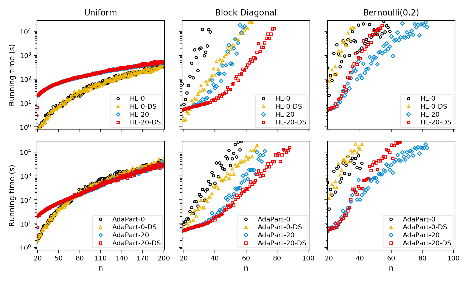
Figure 2: Estimates of expected running times on random instances.

5.1 Tested rejection samplers and approximation schemes

We implemented the following instantiations of DeepAR:

HL-$d$: the scheme due to Huber using the depth-$d$ Huber–Law bound.

AdaPart-$d$: the AdaPart scheme using the depth-$d$ Schrijver–Soules bound.

The time requirement per trial is $O(n^{2})$ for HL-$d$ and $O(n^{3})$ for AdaPart-$d$, provided that there is always a column on which the Schrijver–Soules bound is nesting (Supplement A.3).

We ran the schemes with depths $d\in\{0,20\}$ and with and without preprocessing of the input matrix. The preprocessing is similar to one by Huber and Law Huber2008 : First, we ensure that every entry belongs to at least one permutation of nonzero weight Tassa2012 . Then we apply Sinkhorn balancing $n^{2}$ times Sullivan2014 to obtain a nearly doubly stochastic matrix (Supplement A.2). Finally, we divide each row vector by its largest entry. This preprocessing, we abbreviate as DS, takes $O(n^{4})$ time. When the input matrix was preprocessed in this way, we add the suffix “-DS” to the names HL-$d$ and AdaPart-$d$.

For comparison, we also ran Godsil–Gutman type schemes (our implementations) and the original authors’ implementation of AdaPart. Our main finding is that Godsil–Gutman type schemes are not competitive and that our implementation, AdaPart-$0$, is typically one to two orders of magnitude faster than the original one; see Supplement C for more detailed report on these experiments.

5.2 Estimates of expected running times

We estimated the expected running time (ERT) of the schemes for producing a $(0.1,0.05)$-approximation of the permanent. Using GBAS Huber2017 , this yields a requirement of $388$ accepted samples. To save the total computing time of the study, we estimate the ERT based on $65$ accepted samples. By the argument of Section 2.1, our estimate of the ERT has a relative error at most 50 % with probability at least 95 % (if we ignore the variation in the running times of rejected trials).

We considered three classes of random matrices: in Uniform the entries are independent and distributed uniformly in $[0,1]$; Block Diagonal consists of block diagonal matrices whose diagonal elements are independent $5\times 5$ matrices from Uniform (the last element may be smaller); in Bernoulli$(p)$, the entries are independent taking value $1$ with probability $p$, and $0$ otherwise. We observe (Fig. 2) that on Uniform, deep bounds do not pay off and that the Huber–Law scheme is an order-of-magnitude faster than AdaPart. On Block Diagonal, deep bounds bring a significant, two-orders-of-magnitude boost and AdaPart is slightly faster than Huber–Law; furthermore, DS brings a substantial additional advantage for larger instances (visible as a smaller slope of the log-time plot). Bernoulli$(p)$ again shows the superiority of deep bounds, but also a case where DS is harmful.

We also considered (non-random) benchmark instances. Five of these are from the Network Repository Rossi2015 (http://networkrepository.com, licensed under CC BY-SA), the same as included by Kuck et al. Kuck2019 . In addition, we included Staircase-$n$ instances, which are $(0,1)$-matrices $A=(a_{ij})$ of size $n\times n$ such that $a_{ij}=1$ if and only if $i+j\leq n+2$. Soules Soules2003 mentions these as examples where the ratio of the upper bound and the permanent is particularly large. We observe (Table LABEL:tbl:instance) that on four of the five instances from the repository, the preprocessing has relatively little effect, deep bounds yield a speedup by one to two orders of magnitude, and the configurations of AdaPart and the Huber–Law scheme are about equally fast. The exception is cage5, on which the Huber–Law bound breaks down without DS; a closer inspection reveals that is due to row-sums that are less than $1$. On the Staircase instances, deep bounds yield a dramatic speedup and DS makes a clear difference.

Table 1: Estimates of expected running times (in seconds) on benchmark instances.

		AdaPart-$d$		AdaPart-$d$-DS		HL-$d$		HL-$d$-DS
Instance	$n$	$d=0$	$d=20$	$d=0$	$d=20$	$d=0$	$d=20$	$d=0$	$d=20$
ENZYMES-g192	31	$2\cdot 10^{2}$	$\mathbf{1\cdot 10^{1}}$	$8\cdot 10^{2}$	$\mathbf{1\cdot 10^{1}}$	$1\cdot 10^{2}$	$\mathbf{1\cdot 10^{1}}$	$6\cdot 10^{2}$	$2\cdot 10^{1}$
ENZYMES-g230	32	$3\cdot 10^{2}$	$2\cdot 10^{1}$	$1\cdot 10^{3}$	$\mathbf{1\cdot 10^{1}}$	$2\cdot 10^{2}$	$\mathbf{1\cdot 10^{1}}$	$1\cdot 10^{3}$	$2\cdot 10^{1}$
ENZYMES-g479	28	$3\cdot 10^{2}$	$8\cdot 10^{0}$	$1\cdot 10^{3}$	$8\cdot 10^{0}$	$1\cdot 10^{2}$	$\mathbf{7\cdot 10^{0}}$	$7\cdot 10^{2}$	$9\cdot 10^{0}$
cage5	37	$2\cdot 10^{3}$	$2\cdot 10^{1}$	$1\cdot 10^{3}$	$\mathbf{1\cdot 10^{1}}$	$>10^{4}$	$5\cdot 10^{3}$	$9\cdot 10^{2}$	$2\cdot 10^{1}$
bcspwr01	39	$6\cdot 10^{2}$	$\mathbf{1\cdot 10^{1}}$	$4\cdot 10^{3}$	$2\cdot 10^{1}$	$3\cdot 10^{2}$	$\mathbf{1\cdot 10^{1}}$	$2\cdot 10^{3}$	$2\cdot 10^{1}$
Staircase-30	30	$>10^{4}$	$2\cdot 10^{1}$	$9\cdot 10^{3}$	$8\cdot 10^{0}$	$>10^{4}$	$2\cdot 10^{1}$	$3\cdot 10^{3}$	$\mathbf{7\cdot 10^{0}}$
Staircase-45	45	$>10^{4}$	$>10^{4}$	$>10^{4}$	$2\cdot 10^{3}$	$>10^{4}$	$>10^{4}$	$>10^{4}$	$\mathbf{8\cdot 10^{2}}$

6 Concluding remarks

DeepAR (deep acceptance–rejection) boosts recursive rejection sampling by replacing the basic upper bound by a deep variant. While efficient implementations of DeepAR to concrete problems remain to be discovered case by case, we demonstrated the prospects of the method on the permanent of matrices with nonnegative entries, an extensively studied hard problem. DeepAR enables smooth trading of precomputation for acceptance rate in the rejection sampling, and in our empirical study showed expedition by up to several orders of magnitude, as compared to the recent AdaPart method Kuck2019 (the original authors’ implementation). The speedup varies depending on the size of the matrix and the tightness of the upper bound, and can be explained by three factors. A factor of $10$–$100$ is due to implementation details, including both the different programming language and our more streamlined evaluation of the bounds for submatrices. Another factor of $2$–$1000$ is due to our deep bounds. The third factor is due to the preprocessing of the matrix towards doubly-stochasticity (DS), which yields large savings on some hard instances, being mildy harmful for some others. A topic for further research is automatic selection of the best configuration (the permanent bound, depth, DS) on per-instance basis. There are also intriguing analytic questions (cf. Remark 2).

References

- [1] Dimitris Achlioptas and Pei Jiang. Stochastic integration via error-correcting codes. In Proceedings of the Thirty-First Conference on Uncertainty in Artificial Intelligence, UAI 2015, pages 22–31. AUAI Press, 2015.
- [2] Isabel Beichl and Francis Sullivan. Approximating the permanent via importance sampling with application to the dimer covering problem. J. Comput. Phys., 149(1):128–147, 1999.
- [3] Ivona Bezáková, Daniel Štefankovič, Vijay V. Vazirani, and Eric Vigoda. Accelerating simulated annealing for the permanent and combinatorial counting problems. SIAM J. Comput., 37(5):1429–1454, 2008.
- [4] Andreas Björklund, Thore Husfeldt, Petteri Kaski, and Mikko Koivisto. Evaluation of permanents in rings and semirings. Inf. Process. Lett., 110(20):867–870, 2010.
- [5] Lev M. Brègman. Some properties of nonnegative matrices and their permanents. Dokl. Akad. Nauk, 211(1):27–30, 1973.
- [6] Andrei Z. Broder. How hard is it to marry at random? (on the approximation of the permanent). In Proceedings of the Eighteenth Annual ACM Symposium on Theory of Computing, STOC 1986, pages 50–58. Association for Computing Machinery, 1986.
- [7] Supratik Chakraborty, Kuldeep S. Meel, and Moshe Y. Vardi. Algorithmic improvements in approximate counting for probabilistic inference: From linear to logarithmic SAT calls. In Proceedings of the Twenty-Fifth International Joint Conference on Artificial Intelligence, IJCAI 2016, pages 3569–3576. AAAI Press, 2016.
- [8] Yuguo Chen and Jun Liu. Sequential Monte Carlo methods for permutation tests on truncated data. Stat. Sin, 17(3):857–872, 2007.
- [9] Steve Chien, Lars E. Rasmussen, and Alistair Sinclair. Clifford algebras and approximating the permanent. J. Comput. Syst. Sci., 67(2):263–290, 2003.
- [10] Paul Dagum, Richard M. Karp, Michael Luby, and Sheldon M. Ross. An optimal algorithm for Monte Carlo estimation. SIAM J. Comput., 29(5):1484–1496, 2000.
- [11] Jeffrey Dudek, Dror Fried, and Kuldeep S. Meel. Taming discrete integration via the boon of dimensionality. In Advances in Neural Information Processing Systems, volume 33, pages 1071–1082. Curran Associates, Inc., 2020.
- [12] Stefano Ermon, Carla P. Gomes, Ashish Sabharwal, and Bart Selman. Taming the curse of dimensionality: Discrete integration by hashing and optimization. In Proceedings of the 30th International Conference on Machine Learning, ICML 2013, volume 28 of JMLR Workshop and Conference Proceedings, pages 334–342. JMLR.org, 2013.
- [13] Alan Frieze and Mark Jerrum. An analysis of a Monte Carlo algorithm for estimating the permanent. Combinatorica, 15(1), 1995.
- [14] Martin Fürer and Shiva P. Kasiviswanathan. An almost linear time approximation algorithm for the permanent of a random (0-1) matrix. In Proceedings of the Twenty-Fourth International Conference on Foundations of Software Technology and Theoretical Computer Science, Lecture Notes in Computer Science, volume 3328, pages 263–274. Springer, 2004.
- [15] David G. Glynn. The permanent of a square matrix. Eur. J. Comb., 31(7):1887–1891, 2010.
- [16] Christopher D. Godsil and Ivan Gutman. On the matching polynomial of a graph. In Algebraic Methods in Graph Theory, Colloquia Mathematica Societatis János Bolyai, number 25, pages 241–249. North-Holland, 1981.
- [17] Mark Huber. Exact sampling from perfect matchings of dense regular bipartite graphs. Algorithmica, 44(3):183–193, 2006.
- [18] Mark Huber. A Bernoulli mean estimate with known relative error distribution. Random Struct. Algorithms, 50(2):173–182, 2017.
- [19] Mark Huber and Jenny Law. Fast approximation of the permanent for very dense problems. In Proceedings of the Nineteenth Annual ACM-SIAM Symposium on Discrete Algorithms, SODA 2008, pages 681–689. Society for Industrial and Applied Mathematics, 2008.
- [20] Mark Jerrum and Alistair Sinclair. Approximating the permanent. SIAM J. Comput., 18(6):1149–1178, 1989.
- [21] Mark Jerrum, Alistair Sinclair, and Eric Vigoda. A polynomial-time approximation algorithm for the permanent of a matrix with nonnegative entries. J. ACM, 51(4):671–697, 2004.
- [22] Narendra Karmarkar, Richard Karp, Richard Lipton, Lazlo Lovász, and Michael Luby. A Monte-Carlo algorithm for estimating the permanent. SIAM J. Comput., 22(2):284–293, 1993.
- [23] Jonathan Kuck, Tri Dao, Hamid Rezatofighi, Ashish Sabharwal, and Stefano Ermon. Approximating the permanent by sampling from adaptive partitions. In Advances in Neural Information Processing Systems 32, pages 8860–8871. Curran Associates, Inc., 2019.
- [24] Henryk Minc. Upper bounds for permanents of (0, 1)-matrices. Bull. Amer. Math. Soc, 69(6):789–791, 1963.
- [25] James E. Newman and Moshe Y. Vardi. FPRAS approximation of the matrix permanent in practice. CoRR, abs/2012.03367, 2020.
- [26] Roger Paredes, Leonardo Dueñas-Osorio, Kuldeep S. Meel, and Moshe Y. Vardi. Principled network reliability approximation: A counting-based approach. Reliab. Eng. Syst. Saf., 191:93–110, 2019.
- [27] Lars E. Rasmussen. Approximating the permanent: A simple approach. Random Struct. Algorithms, 5(2):349–362, 1994.
- [28] Ryan A. Rossi and Nesreen K. Ahmed. The network data repository with interactive graph analytics and visualization. In Proceedings of the Twenty-Ninth AAAI Conference on Artificial Intelligence, pages 4292–4293. AAAI Press, 2015.
- [29] Herbert J. Ryser. Combinatorial mathematics, volume 14. Mathematical Association of America, 1963.
- [30] Alexander Schrijver. A short proof of Minc’s conjecture. J. Comb. Theory Ser. A, 25(1):80–83, 1978.
- [31] Peter J. Smith, Hongsheng Gao, and Martin V. Clark. Performance bounds for MMSE linear macrodiversity combining in Rayleigh fading, additive interference channels. J. Commun. Networks, 4(2):102–107, 2002.
- [32] George W. Soules. New permanental upper bounds for nonnegative matrices. Linear Multilinear Algebra, 51(4):319–337, 2003.
- [33] George W. Soules. Permanental bounds for nonnegative matrices via decomposition. Linear Algebra Appl., 393:73–89, 2005.
- [34] Francis Sullivan and Isabel Beichl. Permanents, -permanents and Sinkhorn balancing. Comput. Stat., 29(6):1793–1798, 2014.
- [35] Topi Talvitie, Kustaa Kangas, Teppo Niinimäki, and Mikko Koivisto. A scalable scheme for counting linear extensions. In Proceedings of the Twenty-Seventh International Joint Conference on Artificial Intelligence, IJCAI 2018, pages 5119–5125. ijcai.org, 2018.
- [36] Tamir Tassa. Finding all maximally-matchable edges in a bipartite graph. Theor. Comput. Sci., 423:50–58, 2012.
- [37] Jeffrey K. Uhlmann. Matrix permanent inequalities for approximating joint assignment matrices in tracking systems. J. Frankl. Inst., 341(7):569–593, 2004.
- [38] Leslie G. Valiant. The complexity of computing the permanent. Theor. Comput. Sci., 8(2):189–201, 1979.