Issues with Positivity-Preserving Patankar-type Schemes

Abstract

Patankar-type schemes are linearly implicit time integration methods designed to be unconditionally positivity-preserving. However, there are only little results on their stability or robustness. We suggest two approaches to analyze the performance and robustness of these methods. In particular, we demonstrate problematic behaviors of these methods that, even on very simple linear problems, can lead to undesired oscillations and order reduction for vanishing initial condition. Finally, we demonstrate in numerical simulations that our theoretical results for linear problems apply analogously to nonlinear stiff problems.

AMS subject classification. 65L06, 65L20, 65L04

1 Introduction

Many differential equations in biology, chemistry, physics, and engineering are naturally equipped with constraints such as the positivity of certain solution components (e.g., density, energy, pressure) and conservation (e.g., total mass, momentum, energy). In particular, reaction equations are often of this form. Typically, such reaction systems can also be stiff. We consider such ordinary differential equations (ODEs)

$$u^{\prime}(t)=f(u(t)),\quad u(0)=u_{0},$$ (1)

that can be written as a production destruction system (PDS) [9]

$$f_{i}(u)=\sum_{j\in I}(p_{ij}(u)-d_{ij}(u)),\quad\forall i\in I,$$ (2)

where $p_{ij},d_{ij}\geq 0$ are the production and destruction terms, respectively. Sometimes, these terms are conveniently written as matrices $p(u)=(p_{ij}(u))_{i,j}$ and $d(u)=(d_{ij}(u))_{i,j}$.

Definition 1.1.

An ODE (1) is called positive, if positive initial data $u_{0}>0$ result in positive solutions $u(t)>0,\forall t$. Here, inequalities for vectors are interpreted componentwise, i.e., $u(t)>0$ means $\forall i\in I\colon u_{i}(t)>0$. A production destruction system (2) is called conservative, if $\forall i,j\in I,\forall u\colon p_{ij}(u)=d_{ji}(u)$.

A slight generalization of the PDS (2) is given by the production destruction rest system (PDRS)

$$f_{i}(u)=r_{i}(u)+\sum_{j\in I}(p_{ij}(u)-d_{ij}(u)),\quad\forall i\in I,$$ (3)

where $p_{ij}$, $d_{ij}$ are as before and additional rest terms $r_{i}$ are introduced. These can of course violate the conservative nature of a PDS but can still result in a positive solution if $r_{i}\geq 0$. The rest term can be interpreted as additional force/source term.

The existence, uniqueness and positivity of the solution of a PDS can be proven under the following assumptions [13].

Theorem 1.2.

The PDS with initial conditions $u^{0}\geq 0$ has a unique solution $u\in[\mathcal{C}^{1}(\mathbb{R}^{+})]^{|I|}$ and $u_{i}(t)>0$ if $u_{i}^{0}>0$, if

1. for all $i,j\in I$ $d_{ij}$ is locally Lipschitz continuous in $\mathbb{R}^{|I|}$,

2. $d_{ij}(u)=0$ for all $i,j\in I$ if $u=0$,

3. $d_{ij}(u)=\tilde{d}_{ij}(u)u_{i}$ with $\tilde{d}_{ij}\in\mathcal{C}((\overline{\mathbb{R}^{+}})^{|I|})$ and $\tilde{d}_{ij}(u)>0$ if $u>0$ and $\tilde{d}_{ij}(u)=0$ if $u=0$.

In [9] the previous assumptions 2 and 3 are replaced by the condition $d_{ij}(u)\to 0$ if $u_{i}\to 0$. It can be easily shown that this condition plus the Lipschitz continuity of the destruction terms lead to similar structures. Let $C$ be the maximum of the Lipschitz continuity constants of the destruction terms and consider $u=v$ except for the $i$-th component for which $v_{i}=0$ and, hence, $d_{ij}(v)=0$ for the new condition. We have that

$$0\leq\,d_{ij}(u)=|d_{ij}(u)-d_{ij}(v)|\leq C||u-v||_{2}=Cu_{i}.$$ (4)

Hence, we can define

$$\tilde{d}_{ij}(u)\mathrel{\mathop{\ordinarycolon}}=\frac{d_{ij}(u)}{u_{i}}\leq C.$$ (5)

This condition is less restrictive and it does not guarantee the continuity of $\tilde{d}_{ij}$ in $u_{i}=0$. For the rest of the paper, we will consider assumptions of Theorem 1.2. Also, all the physically/chemically/biologically relevant cases, of which we are aware, fall in this definition.

To ensure physically meaningful and robust numerical approximations, we would like to preserve positivity and conservation discretely.

Definition 1.3.

A numerical method computing $u^{n+1}\approx u(t_{n+1})$ given $u^{n}\approx u(t_{n})$ is called conservative, if $\sum_{i}u^{n+1}_{i}=\sum_{i}u^{n}_{i}$. It is called unconditionally positive, if $u^{n}>0$ implies $u^{n+1}>0$.

There are several ways to study positivity of numerical methods [12], e.g., based on the concept of strong stability preserving (SSP) [15] or adaptive Runge–Kutta (RK) methods [36]. However, general linear methods are restricted to conditional positivity if they are at least second order accurate [6]. One way to circumvent such order restrictions is given by diagonally split RK methods, which can be unconditionally positive [21, 4, 18]. However, they are less accurate than the unconditionally positive implicit–Euler method for large step sizes in practice [30, 6].

Another approach to unconditionally positivity-preserving methods is based on the so-called Patankar trick [38, Section 7.2-2]. First- and second-order accurate conservative methods based thereon were introduced in [9]. Later, these were extended to families of second- and third-order accurate modified Patankar–Runge–Kutta (MPRK) methods based on the Butcher coefficients [26, 28] and the Shu–Osher form [19, 20]. Related deferred correction (DeC) methods were proposed recently [37]. Positive but not conservative methods using the Patankar trick have been proposed and studied in [10], although the connection to Patankar methods seems to be unknown up to now. Other related numerical schemes are inflow-implicit/outflow-explicit methods [34, 35, 14]. Ideas from Patankar-type methods have also been used in numerical methods based on limiters [29].

The methods mentioned above are based on explicit RK methods. To guarantee positivity, the schemes are modified to be linearly implicit, which seems to introduce some stabilization mechanism. In fact, Patankar-type methods have been applied successfully to some stiff systems [26, 28, 25, 10]. Recently, Patankar methods have been investigated using Lyapunov stability theory [22, 24, 23]. We will point out the relation between their approach and our investigations. Lately, BBKS and GeCo, two geometric integrators, have been introduce to simulate biochemistry models preserving not only positivity and conservation, but also all linear invariants of a system [31, 8, 2, 7].

1.1 Motivating example

Consider the normal linear system

$$u^{\prime}(t)=10^{2}\begin{pmatrix}-1&1\\ 1&-1\end{pmatrix}u(t),\quad u(0)=u_{0}=\begin{pmatrix}0.1\\ 0\end{pmatrix},$$ (6)

which can be written as a production destruction system with

$$p(u)=\begin{pmatrix}0&10^{2}u_{2}\\ 10^{2}u_{1}&0\end{pmatrix},\quad d(u)=\begin{pmatrix}0&10^{2}u_{1}\\ 10^{2}u_{2}&0\end{pmatrix}.$$ (7)

On (6), we can show different problematic behaviors. We solve (6) with several different methods. In detail, we apply the second order method SI-RK2 of [10], the second- and third-order accurate modified Patankar–Runge–Kutta schemes MPRK(2,2,$\alpha$) and MPRK(4,3,$\alpha$,$\beta$) from [26, 28] with different parameter selections, the implicit Midpoint rule and fifth-order, three stage RadauIIA5 scheme [17] implemented in DifferentialEquations.jl [40] in Julia [5]. The solutions are shown in Figure 1(a). It can be recognized that even for this simple test case, most of the methods are oscillating for the selected time step but with different amplitudes while RadauIIA5 results in an oscillation–free approximation. We will see that there is a connection between positivity and oscillation–free linear schemes.
Another problem rises if we use other Patankar schemes. These methods are constructed for strictly positive PDS, therefore we have to substitute the zero initial condition with something very small, e.g. $u_{2}(0)=10^{-250}$. We observe in Figure 1(b) that some of the methods replicate the initial condition for some time steps while others do not leave it at all in the considered time interval. On the other side classical implicit Runge–Kutta method as well as other modified Patankar schemes do not show this behavior and their first time step approaches quickly the steady state value. This issue is linked with a loss of accuracy in the limit for an initial condition approaching zero.
In our investigation, we want to find the Patankar methods that have those undesirable behaviors and avoid them.

(a) $\Delta t=0.05$

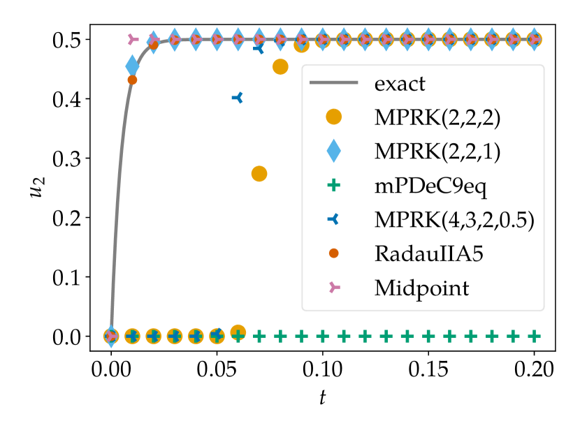
(b) $\Delta t=0.01$

Figure 1: Numerical solutions of the normal linear system (6) with real and non-positive eigenvalues obtained using different Patankar-type schemes as well as two implicit Runge–Kutta methods (only second component depicted) with initial condition $u_{0}=(1,10^{-250})^{T}$.

Remark 1.4.

A stability theory for Patankar type methods is still under development and only few preliminary results have been presented. Recently, in [22, 24, 23] a promising ansatz to investigate the behavior of conservative and positivity preserving methods has been proposed. In their work, the main idea is to use the center manifold theory corresponding to fixed-point investigations. First applied on $2\times 2$ systems in [22], the theory has been extended to general $n\times n$ systems in [23]. The main idea is the following: a generic linear system $y^{\prime}=Ay$ with $A\in\mathbb{R}^{n\times n}$ with initial condition $y_{0}>0$ possessing $k>0$ linear invariants is considered. In such a case, zero is always an eigenvalue of $A$ which implies the existence of nontrivial steady state solutions, cf. [23]. The steady state solutions are fixed-points for any reasonable time integration method. Due to the nonlinear character of Patankar-type schemes (actually for all higher-order positivity preserving schemes), a nonlinear iteration process is obtained. Here, additional techniques have to be used to investigate the stability properties. The authors of [22, 24, 23] proved a theorem based on the central manifold theorem which gives sufficient conditions for the stability of all such methods. It is further demonstrated that MPRK22($\alpha)$ is stable for all $\Delta t>0$, i.e., it will converge to such fixed-points at any rate.
As shown in [22], we suspect that most of modified Patankar schemes are stable in the fixed-point sense. In our investigation, we do not deal with this type of stability, but, rather, we look for some more restricted schemes that show monotone character for monotone problems and that do not completely lose the high order accuracy. A stability analysis of all the considered methods with respect to the method proposed in [23] is work in progress. Furthermore, the connection between our observations and the obtained eigenvalues of the iterative process will be considered and compared in the future.

1.2 Scope of the article

Motivated by our numerical examples above we are interested in concepts that detect the dominant appearance of spurious oscillations and the loss of accuracy in the limit of an initial condition going to zero. We have focused on different types of systems (stiff, dissipative ones, etc.) and considered several quantities like the dissipation of some norms or Lyapunov functionals, cf. [43, 41, 42, 44, 45]. However, the obtained results have not been sufficient for us to describe the properties of the schemes in an adequate way. Thus, we will directly measure the amount of spurious oscillations using a generic $2\times 2$ linear system as a test problem, and focus as well as on the loss of accuracy in the limit process. Our investigation leads to a deeper understanding of the basic properties of Patankar-type methods.

The rest of the article is structured as follows. The numerical schemes studied in this article are introduced in Section 2. In Section 3, we describe the linear problem on which the methods will be studied. Thereafter, in Section 4, we show the connection between oscillations and positivity for linear problems and linear schemes, then we study the oscillation–free property for RK schemes and for a MPRK scheme. We continue with an analytical investigation on the loss of the order of accuracy in the limit of vanishing initial condition in Section 5. In Section 6, a numerical study on linear systems derives the results on bounds on time step for oscillation–free schemes for all other Patankar schemes. In Section 7, we extend the numerical study to nonlinear and stiff problems. Finally, we summarize and discuss our results in Section 8.

2 Numerical schemes

Here, we introduce Patankar-type methods proposed in the literature that we will investigate later. In addition, we propose a new MPRK method and give a heuristic on how to construct such schemes in general.

2.1 Modified Patankar–Euler method

The explicit Euler method $u^{n+1}=u^{n}+\Delta tf(u^{n})$ can be modified by the Patankar trick [38, Section 7.2-2] for a PDR system (3) to get the positive Patankar–Euler method

$$u^{n+1}_{i}=u^{n}_{i}+\Delta tr_{i}\bigl{(}u^{n}\bigr{)}+\Delta t\sum_{j}\left(p_{ij}\bigl{(}u^{n}\bigr{)}-d_{ij}\bigl{(}u^{n}\bigr{)}\frac{u^{n+1}_{i}}{u^{n}_{i}}\right).$$ (8)

Indeed, given $r,p,d\geq 0$, the new numerical solution $u^{n+1}$ is obtained by solving a linear system with positive diagonal entries, vanishing off-diagonal entries, and a positive right-hand side.

Since the Patankar–Euler method (8) is not conservative, the modified Patankar–Euler method

$$u^{n+1}_{i}=u^{n}_{i}+\Delta tr_{i}\bigl{(}u^{n}\bigr{)}+\Delta t\sum_{j}\left(p_{ij}\bigl{(}u^{n}\bigr{)}\frac{u^{n+1}_{j}}{u^{n}_{j}}-d_{ij}\bigl{(}u^{n}\bigr{)}\frac{u^{n+1}_{i}}{u^{n}_{i}}\right)$$ (MPE)

has been introduced in [9] (with additional rest terms $r$ here). The modification of the production terms makes the method conservative if the rest terms $r$ vanish. Nevertheless, the method is still positive, because the arising linear systems has positive diagonal entries, negative off-diagonal entries, and is strictly diagonally dominant. Hence, the system matrix is an $M$ matrix and, since the right-hand side is positive, the solution $u^{n+1}$ is positive [3, Section 6.1]. We observe that, when dealing with the scalar linear test problem $u^{\prime}=\lambda u$ with $\lambda<0$, the Patankar–Euler method coincides with the implicit–Euler method. Similarly, MPE coincides with the implicit–Euler method if we deal with positive and conservative linear PDS. Indeed, the destruction terms $d_{i}(u)=\sum_{j}d_{ij}(u)$ must go to 0 if $u_{i}\to 0$ [9]. Since the system is linear, $d_{ij}(u^{n})=\tilde{d}_{ij}u_{i}^{n}$ with $\tilde{d}_{ij}\in\mathbb{R}^{+}_{0}$. Exploiting the conservation properties, we have $p_{ji}(u^{n})=\tilde{d}_{ij}u^{n}_{i}$. Substituting these formulae in MPE leads to the implicit–Euler method.

2.2 MPRK methods using Butcher coefficients

A one-parameter family of MPRK schemes based on the Butcher coefficients of a two stage, second-order RK method was introduced in [26]. Given a parameter $\alpha\in[1/2,\infty)$, the method is

$$y^{1} =u^{n}, \alpha$$ (MPRK(2,2,))

$$y^{2}_{i} =u^{n}_{i}+\alpha\Delta tr_{i}\bigl{(}y^{1}\bigr{)}+\alpha\Delta t\sum_{j}\left(p_{ij}\bigl{(}y^{1}\bigr{)}\frac{y^{2}_{j}}{y^{1}_{j}}-d_{ij}\bigl{(}y^{1}\bigr{)}\frac{y^{2}_{i}}{y^{1}_{i}}\right),$$

$$u^{n+1}_{i} =u^{n}_{i}+\Delta t\left(\frac{2\alpha-1}{2\alpha}r_{i}\bigl{(}y^{1}\bigr{)}+\frac{1}{2\alpha}r_{i}\bigl{(}y^{2}\bigr{)}\right)$$

$$\qquad+\Delta t\sum_{j}\Biggl{(}\left(\frac{2\alpha-1}{2\alpha}p_{ij}\bigl{(}y^{1}\bigr{)}+\frac{1}{2\alpha}p_{ij}\bigl{(}y^{2}\bigr{)}\right)\frac{u^{n+1}_{j}}{(y^{2}_{j})^{1/\alpha}(y^{1}_{j})^{1-1/\alpha}}$$

$$\qquad\qquad\qquad-\left(\frac{2\alpha-1}{2\alpha}d_{ij}\bigl{(}y^{1}\bigr{)}+\frac{1}{2\alpha}d_{ij}\bigl{(}y^{2}\bigr{)}\right)\frac{u^{n+1}_{i}}{(y^{2}_{i})^{1/\alpha}(y^{1}_{i})^{1-1/\alpha}}\Biggr{)}.$$

The scheme for the choice $\alpha=1$ is based on Heun’s method and has been proposed already in [9]. Heun’s method can be also written as a strong stability preserving Runge–Kutta method (SSPRK) and we will denote it by SSPRK(2,2) [15].

A similar two-parameter family MPRK(4,3,$\alpha$,$\beta$) of four stage, third-order accurate schemes was introduced and studied in [28, 27]. The family under consideration can be found in the A for completeness.

2.3 MPRK methods using Shu–Osher coefficients

A two-parameter family of MPRK schemes based on the Shu–Osher coefficients of a two stage, second-order RK method was introduced in [19]. Given parameters $\alpha,\beta$, the method is

$$y^{1} =u^{n}, \alpha \beta$$ (MPRKSO(2,2,,))

$$y^{2}_{i} =y^{1}_{i}+\beta\Delta tr_{i}\bigl{(}y^{1}\bigr{)}+\beta\Delta t\sum_{j}\left(p_{ij}\bigl{(}y^{1}\bigr{)}\frac{y^{2}_{j}}{y^{1}_{j}}-d_{ij}\bigl{(}y^{1}\bigr{)}\frac{y^{2}_{i}}{y^{1}_{i}}\right),$$

$$u^{n+1}_{i} =(1-\alpha)y^{1}_{i}+\alpha y^{2}_{i}+\Delta t\left((1-\frac{1}{2\beta}-\alpha\beta)r_{i}\bigl{(}y^{1}\bigr{)}+\frac{1}{2\beta}r_{i}\bigl{(}y^{2}\bigr{)}\right)$$

$$\qquad+\Delta t\sum_{j}\Biggl{(}\left((1-\frac{1}{2\beta}-\alpha\beta)p_{ij}\bigl{(}y^{1}\bigr{)}+\frac{1}{2\beta}p_{ij}\bigl{(}y^{2}\bigr{)}\right)\frac{u^{n+1}_{j}}{(y^{2}_{j})^{\gamma}(y^{1}_{j})^{1-\gamma}}$$

$$\qquad\qquad\qquad-\left((1-\frac{1}{2\beta}-\alpha\beta)d_{ij}\bigl{(}y^{1}\bigr{)}+\frac{1}{2\beta}d_{ij}\bigl{(}y^{2}\bigr{)}\right)\frac{u^{n+1}_{i}}{(y^{2}_{i})^{\gamma}(y^{1}_{i})^{1-\gamma}}\Biggr{)},$$

where the parameters are restricted to $\alpha\in[0,1]$, $\beta\in(0,\infty)$, $\alpha\beta+\frac{1}{2\beta}\leq 1$, and

$$\gamma=\frac{1-\alpha\beta+\alpha\beta^{2}}{\beta(1-\alpha\beta)},$$ (9)

in order to be positive. In our simulations, we will exchange the weights of production and destruction when the coefficients are negative. In the next section we will give an example of such inversion. An extension to four stage, third-order accurate methods MPRKSO(4,3) was developed in [20] and can be found in the A.

2.4 Modified Patankar deferred correction schemes

Arbitrarily high order conservative and positive modified Patankar deferred correction schemes (mPDeC) were introduced in [37]. A time step $[t^{n},t^{n+1}]$ is divided into $M$ sub-intervals, where $t^{n,0}=t^{n}$ and $t^{n,M}=t^{n+1}$. For every sub-interval, the Picard-Lindelöf theorem is mimicked. At each sub-time step $t^{n,m}$, an approximation $y^{m}$ is calculated. In the formulation of [1] an iterative procedure of $K$ correction steps improves the approximation by one order of accuracy at each iteration. The modified Patankar trick is introduced inside the basic scheme to guarantee positivity and conservation of the intermediate approximations. Using the fact that initial states $y_{i}^{0,(k)}=u_{i}^{n}$ are identical for any correction $k$, the mPDeC correction steps can be rewritten for $k=1,\dots,K$, $m=1,\dots,M$ and $\forall i\in I$ as

$$\begin{split}&y_{i}^{m,(k)}-y^{0}_{i}-\sum_{r=0}^{M}\theta_{r}^{m}\Delta tr_{i}\bigl{(}y^{r,(k-1)}\bigr{)}-\\ &\sum_{l=0}^{M}\theta_{l}^{m}\Delta t\sum_{j=1}\left(p_{ij}(y^{l,(k-1)})\frac{y^{m,(k)}_{\gamma(j,i,\theta_{r}^{m})}}{y_{\gamma(j,i,\theta_{l}^{m})}^{m,(k-1)}}-d_{ij}(y^{l,(k-1)})\frac{y^{m,(k)}_{\gamma(i,j,\theta_{l}^{m})}}{y_{\gamma(i,j,\theta_{l}^{m})}^{m,(k-1)}}\right)=0,\end{split}$$ (mPDeC)

where $\theta_{r}^{m}$ are the correction weights and the $\gamma(j,i,\theta_{r}^{m})$ takes value $j$ if $\theta_{r}^{m}>0$ and $i$ otherwise, see [37] for details. This allows to obtain always positive terms in the diagonal terms and nonpositive in the offdiagonal terms of the system matrix. Finally, the new numerical solution is $u_{i}^{n+1}=y_{i}^{M,(K)}$.

The choice of the distribution and the number of sub-time steps $M$ and the number of iterations $K$ determines the order of accuracy of the scheme. In the following, we will compare equispaced and Gauss–Lobatto points. To reach order $d$, we use $M=d-1$ sub-intervals and $K=d$ corrections. We will denote the $p$th-order mPDeC method as mPDeC$p$. Note that mPDeC1 is equivalent to MPE and mPDeC2 is equivalent to MPRK(2,2,1).

2.5 A new MPRK method

We propose the following new three stage, second-order MPRK method based on SSPRK(3,3):

$$y^{1}_{i} =u^{n}_{i},$$ (MPRK(3,2))

$$y^{2}_{i} =u^{n}_{i}+\Delta tr_{i}\bigl{(}y^{1}\bigr{)}+\Delta t\sum_{j}\left(p_{ij}\bigl{(}y^{1}\bigr{)}\frac{y^{2}_{j}}{y^{1}_{j}}-d_{ij}\bigl{(}y^{1}\bigr{)}\frac{y^{2}_{i}}{y^{1}_{i}}\right),$$

$$y_{i}^{3} =u^{n}_{i}$$

$$+\Delta t\frac{r_{i}\bigl{(}y^{1}\bigr{)}+r_{i}\bigl{(}y^{2}\bigr{)}}{4}+\Delta t\sum_{j}\left(\frac{p_{ij}\bigl{(}y^{1}\bigr{)}+p_{ij}\bigl{(}y^{2}\bigr{)}}{4}\frac{y^{3}_{j}}{y^{2}_{j}}-\frac{d_{ij}\bigl{(}y^{1}\bigr{)}+d_{ij}\bigl{(}y^{2}\bigr{)}}{4}\frac{y^{3}_{i}}{y^{2}_{i}}\right),$$

$$u^{n+1}_{i} =u^{n}_{i}+\Delta t\frac{r_{i}\bigl{(}y^{1}\bigr{)}+r_{i}\bigl{(}y^{2}\bigr{)}+4r_{i}\bigl{(}y^{3}\bigr{)}}{6}$$

$$+\Delta t\sum_{j}\Biggl{(}\frac{p_{ij}\bigl{(}y^{1}\bigr{)}+p_{ij}\bigl{(}y^{2}\bigr{)}+4p_{ij}\bigl{(}y^{3}\bigr{)}}{6}\frac{u^{n+1}_{j}}{y^{2}_{j}}$$

$$\qquad\qquad-\frac{d_{ij}\bigl{(}y^{1}\bigr{)}+d_{ij}\bigl{(}y^{2}\bigr{)}+4d_{ij}\bigl{(}y^{3}\bigr{)}}{6}\frac{u^{n+1}_{i}}{y^{2}_{i}}\Biggr{)}.$$

For explicitly time-dependent problems, the abscissae are the ones of SSPRK(3,3) [15], i.e., $c=(0,1,0.5)$. As will be seen later, this scheme has some desirable robustness. MPRK(3,2) is second-order accurate. We will not provide a formal proof of the accuracy of the scheme. Nevertheless we summarize the reasons of the accuracy of each stage. The second stage
$y_{i}^{2}=u_{i}(t^{n+1})+\mathcal{O}(\Delta t^{2})$ is an approximation of order one and we can observe that the ratios $\frac{y^{2}_{i}}{y^{1}_{i}}=1+\mathcal{O}(\Delta t)$ do not further decrease the accuracy since they are multiplied by $\Delta t$. The third stage is as well a first order approximation $y^{3}_{i}=u_{i}(t^{n}+\Delta t/2)+\mathcal{O}(\Delta t^{2}).$ Indeed, even if the midpoint rule is a second order quadrature formula, the ratios $\frac{y_{i}^{3}}{y_{i}^{2}}=\frac{u_{i}(t^{n}+\Delta t/2)+\mathcal{O}(\Delta t^{2})}{u_{i}(t^{n}+\Delta t)+\mathcal{O}(\Delta t^{2})}=1+\mathcal{O}(\Delta t).$ In the final stage, the Simpson rule is applied, where we get only second order accuracy since $y^{2}$ and $y^{3}$ carry a first order error with them. Hence,

$$u^{n+1}_{i}=u_{i}(t^{n+1})+\mathcal{O}(\Delta t^{3}),$$

and this gives us ratios $\frac{u^{n+1}_{i}}{y^{2}_{i}}=\frac{u_{i}(t^{n+1})+\mathcal{O}(\Delta t^{3})}{u_{i}(t^{n+1})+\mathcal{O}(\Delta t^{2})}=1+\mathcal{O}(\Delta t^{2})$ which are multiplied by $\Delta t$. At the end, the scheme is second-order accurate.

Remark 2.1.

The construction of higher-order MPRK schemes can be done in a similar way. The basic idea is to create a method with increasing stage order, similar to the construction of mPDeC. Starting from a high order RK scheme, by applying the modified Patankar trick in the substeps in combination with quadrature rules should lead to high order modified Patankar RK schemes. Essential in the construction is the fact that more stages have to be applied compared to classical RK schemes. This is in accordance with the result of [27] on the existence of third-order, three stages MPRK schemes. There is work in progress to describe a general recipe to construct MPRK schemes of arbitrary order and to study the properties of these schemes.

2.6 Semi-implicit methods

The semi-implicit methods of [10] are also based on the Shu–Osher representation of SSPRK methods, which can be decomposed into convex combinations of the previous step value and explicit Euler steps. Instead of introducing Patankar weights multiplying all destruction terms for a step/stage update, a Patankar weight is introduced for the destruction terms of each Euler stage which is used to compute the new value. Since this procedure limits the order of accuracy of the resulting scheme to first order, an additional function evaluation is used to correct the final solution and get second order of accuracy.

The two methods proposed in [10] are

$$y^{1} =u^{n},$$ (SI-RK2)

$$y^{2}_{i} =\frac{u^{n}_{i}+\Delta tr_{i}(y^{1})+\Delta t\sum_{j}p_{ij}(y^{1})}{1+\Delta t\sum_{j}d_{ij}(y^{1})/y^{1}_{i}},$$

$$y^{3}_{i} =\frac{1}{2}u^{n}_{i}+\frac{1}{2}\frac{y^{2}_{i}+\Delta tr_{i}(y^{2})+\Delta t\sum_{j}p_{ij}(y^{2})}{1+\Delta t\sum_{j}d_{ij}(y^{2})/y^{2}_{i}},$$

$$u^{n+1}_{i} =\frac{y^{3}_{i}+\Delta t^{2}\bigl{(}r_{i}(y^{3})+\sum_{j}p_{ij}(y^{3})\bigr{)}\sum_{j}d_{ij}(y^{3})/y^{3}_{i}}{1+\bigl{(}\Delta t\sum_{j}d_{ij}(y^{3})/y^{3}_{i}\bigr{)}^{2}},$$

which uses three stages and is based on SSPRK(2,2), and

$$y^{1} =u^{n},$$ (SI-RK3)

$$y^{2}_{i} =\frac{u^{n}_{i}+\Delta tr_{i}(y^{1})+\Delta t\sum_{j}p_{ij}(y^{1})}{1+\Delta t\sum_{j}d_{ij}(y^{1})/y^{1}_{i}},$$

$$y^{3}_{i} =\frac{3}{4}u^{n}_{i}+\frac{1}{4}\frac{y^{2}_{i}+\Delta tr_{i}(y^{2})+\Delta t\sum_{j}p_{ij}(y^{2})}{1+\Delta t\sum_{j}d_{ij}(y^{2})/y^{2}_{i}},$$

$$y^{4}_{i} =\frac{1}{3}u^{n}_{i}+\frac{2}{3}\frac{y^{3}_{i}+\Delta tr_{i}(y^{3})+\Delta t\sum_{j}p_{ij}(y^{3})}{1+\Delta t\sum_{j}d_{ij}(y^{3})/y^{3}_{i}},$$

$$u^{n+1}_{i} =\frac{y^{4}_{i}+\Delta t^{2}\bigl{(}r_{i}(y^{4})+\sum_{j}p_{ij}(y^{4})\bigr{)}\sum_{j}d_{ij}(y^{4})/y^{4}_{i}}{1+\bigl{(}\Delta t\sum_{j}d_{ij}(y^{4})/y^{4}_{i}\bigr{)}^{2}},$$

which uses four stages and is based on SSPRK(3,3).

The relation to Patankar schemes becomes obvious by rewriting the computation of the stage $y^{2}$ of (SI-RK2) as

$$y^{2}_{i}=u^{n}_{i}+\Delta tr_{i}(y^{1})+\Delta t\sum_{j}\left(p_{ij}(y^{1})-d_{ij}(y^{1})\frac{y^{2}_{i}}{y^{1}_{i}}\right),$$ (10)

which is the Patankar–Euler method (8). As for the Patankar–Euler method, the semi-implicit methods of [10] are not conservative, i.e., it is not guaranteed that $\sum_{i}u^{n}_{i}=\sum_{i}u^{n+1}_{i}$ when the system is conservative.

2.7 Steady state preservation

Motivated by the investigations of [10], steady state preservation for (modified) Patankar methods will be studied here. Except for the SI-RK2 and SI-RK3 methods [10], such investigations cannot be found in the literature.

Definition 2.2.

A method is steady state preserving if, given a time step $\Delta t$ and $u^{n}=u^{*}$ with $r_{i}(u^{*})+\sum_{j}p_{ij}(u^{*})-d_{ij}(u^{*})=0$, then $u^{n+1}=u^{n}=u^{*}$.

Proposition 2.3.

All (modified) Patankar methods described above are steady state preserving.

Proof.

The solution to each stage and the new step value are unique. If the initial condition is a steady state, this steady state is also a valid solution to all stage and step equations. Indeed, the Patankar weights reduce to 1 and the simple rest-production-destruction forms remains and their sum is 0 in the steady state. Hence, the steady state is preserved. ∎

This theorem is important, since some related modifications of explicit Runge–Kutta methods such as IMEX methods are not necessarily steady state preserving [10]. For (stiff) systems with an initial condition near a steady state, the ability to preserve this steady state exactly is desirable and usually results in a better approximation of solutions nearby or decaying to steady state.

In our discussion, it will be useful to check not only the preservation of the steady state, but also how this state is approached, for example, if in a monotone manner or not.

3 The simplest production destruction system

In order to study the issues observed in Figure 1, we will consider the simplest production destruction system that one can build. For ODE solvers, it is always useful to study Dahlquist’s equation as any linearized (and diagonalizable) system can be recast into several of these equations. Unfortunately, Dahlquist’s equation is not a PDS. We propose to use a $2\times 2$ linear system similar to (6) as test problem. This is the simplest PDS that can be considered. More precisely, we consider the general $2\times 2$ production-destruction linear system as also done lately in similar form in [22]

$$\begin{pmatrix}u_{1}^{\prime}\\ u_{2}^{\prime}\end{pmatrix}=\begin{pmatrix}-a&b\\ a&-b\end{pmatrix}\begin{pmatrix}u_{1}\\ u_{2}\end{pmatrix}.$$ (11)

Rescaling the time, we can simplify this system to a one parameter system setting $a+b=1$ and $0\leq\theta=a\leq 1$, i.e.,

$$\begin{pmatrix}u_{1}^{\prime}\\ u_{2}^{\prime}\end{pmatrix}=\begin{pmatrix}-\theta&(1-\theta)\\ \theta&-(1-\theta)\end{pmatrix}\begin{pmatrix}u_{1}\\ u_{2}\end{pmatrix}.$$ (12)

We can also rescale any initial condition $u^{0}=(u^{0}_{1},u^{0}_{2})^{T}$ to sum up to one (scaling by a factor $\frac{1}{u_{1}^{0}+u_{2}^{0}}$). Thus, we consider the initial condition

$$\begin{pmatrix}u_{1}^{0}\\ u_{2}^{0}\end{pmatrix}=\begin{pmatrix}1-\varepsilon\\ \varepsilon\end{pmatrix}$$ (13)

with $0<\varepsilon<1$. The exact solution of the problem is

$$\begin{pmatrix}u_{1}(t)\\ u_{2}(t)\end{pmatrix}=\begin{pmatrix}(1-\theta)+(\theta-\varepsilon)e^{-t}\\ \theta+(\varepsilon-\theta)e^{-t}\end{pmatrix},$$ (14)

and the steady state of the system is $u^{*}=(1-\theta,\theta)^{T}$.

It is interesting to rewrite the system (12) in its diagonal form to highlight its connection with Dahlquist’s equation. To do so, let us put it into a matrix formulation

$$u^{\prime}=Mu=\begin{pmatrix}-\theta&(1-\theta)\\ \theta&-(1-\theta)\end{pmatrix}u,$$ (15)

we can obtain the diagonal form $M=L^{-1}\Lambda L$ of the system, i.e.,

$$\Lambda=\begin{pmatrix}-1&0\\ 0&0\end{pmatrix};\quad L=\begin{pmatrix}\theta&-(1-\theta)\\ 1&1\end{pmatrix};\quad L^{-1}=\begin{pmatrix}1&1-\theta\\ -1&\theta\end{pmatrix}.$$ (16)

So for $v=Lu$ we can write an always positive (or always negative) exact solution for the first component

$$v_{1}=\theta u_{1}-(1-\theta)u_{2};\qquad v_{1}^{\prime}=-v_{1};\quad v_{1}=e^{-t}v_{1}^{0}.$$ (17)

Indeed, this component is the solution of Dahlquist’s equation, while the second component $v_{2}=u_{1}+u_{2}$ fulfills $v_{2}^{\prime}=0$ and corresponds to the conservation property.

The positivity of $v_{1}=\theta u_{1}-(1-\theta)u_{2}$ in case $\theta u_{1}^{0}-(1-\theta)u_{2}^{0}>0$, i.e., $\frac{u_{1}^{0}}{u_{2}^{0}}>\frac{1-\theta}{\theta}$, is equivalent to say that

$$\frac{u_{1}(t)}{u_{2}(t)}>\frac{1-\theta}{\theta}\Longleftrightarrow u_{2}(t)<\theta=u_{2}^{*}$$ (18)

holds true for all times. This condition means that the solution does not overshoot the asymptotic steady state. This property guarantees the monotonicity of the solution. In the next section, we will see how violating this condition leads to oscillations around the asymptotic steady state.

4 Oscillation–free schemes for linear problems

Now, let us reconsider the system (12). In this section we try to find schemes that do not show oscillatory behavior as the ones presented in Figure 1(a). This reduces to finding schemes that for every $u^{n}$ and every system defined through $0<\theta<1$ have a monotone behavior and do not overshoot/undershoot the steady state solution. In particular, we define two properties that the schemes have to fulfill not to oscillate. We focus on the case $\varepsilon<\theta$ as the opposite one can be obtained switching the two components of the system (12).

Property 4.1 (Not overshooting the steady state).

A method is not overshooting the steady state of (12) if $u^{1}_{2}<\theta$ and $u_{1}^{1}>(1-\theta)$ given any initial state $u^{0}=(1-\varepsilon,\varepsilon)$ with $\varepsilon<\theta$, while when $\varepsilon>\theta$ the method is not overshooting the steady state if $u^{1}_{2}>\theta$ and $u_{1}^{1}<(1-\theta)$.

Property 4.2 (Correct direction).

A method is evolving in the correct direction for system (12) if $u^{1}_{2}>\varepsilon$ and $u_{1}^{1}<(1-\varepsilon)$ given any initial state $u^{0}=(1-\varepsilon,\varepsilon)$ with $\varepsilon<\theta$, while when $\varepsilon>\theta$ the method is evolving in the correct direction if $u^{1}_{2}<\varepsilon$ and $u_{1}^{1}>(1-\varepsilon)$.

In the following we will focus mainly on Property 4.1. Indeed, a similar analysis can be conduct to check when Property 4.2 is preserved and we put it in B. Moreover, we have observed that in very few occasions the approximation moves in the wrong direction, i.e., if $\varepsilon<\theta$ we rarely have that $u_{2}^{1}<\varepsilon$. The interesting condition is $u_{2}<\theta$, or, equivalently $\frac{u_{2}}{u_{1}}<\frac{\theta}{(1-\theta)}$. We have already shown that this condition is equivalent to preserving the positivity of the first component of the diagonalized system (17).

Proposition 4.3 (Oscillation-free and positive Runge-Kutta methods).

Consider the linear system (12) with $\varepsilon<\theta$. For a linear method such as RK methods, the positivity of $v_{1}^{n}=\theta u_{1}^{n}-(1-\theta)u_{2}^{n}$ is equivalent to not overshooting Property 4.1, i.e., $\theta=u_{2}^{*}>u_{2}^{n}\Longleftrightarrow(1-\theta)=u_{1}^{*}<u_{1}^{0}$. Similarly, in case $\varepsilon>\theta,$ the negativity of $v_{1}^{n}$ is equivalent to the Property 4.1 condition, i.e., $\theta=u_{2}^{*}<u_{2}^{n}\Longleftrightarrow(1-\theta)=u_{1}^{*}>u_{1}^{0}$.

Proof.

First of all, let us notice that in case $\varepsilon<\theta$, we have that $v_{1}^{0}=\theta u_{1}^{0}-(1-\theta)u_{2}^{0}=\theta(1-\varepsilon)-(1-\theta)\varepsilon>0$. Let us consider a RK scheme in Einstein’s notation, denoting the $s$th RK stage with $y_{i}^{(s)}$ and with $A,\,b,\,c$ the usual RK matrix and vectors [16]. The RK method for the system (12) can be written as

$$y^{(s)}_{i}=u_{i}^{n}+\Delta tM^{j}_{i}A^{s}_{k}y_{j}^{(k)}$$ (19)

$$u^{n+1}_{i}=u_{i}^{n}+\Delta tb_{s}M^{j}_{i}y_{j}^{(s)},$$ (20)

where $M$ is the matrix in (15). Now, premultiplying by $L$ defined in (16) we obtain the same RK method for the diagonalized system, i.e.,

$$w^{(s)}_{\ell}\mathrel{\mathop{\ordinarycolon}}=L_{\ell}^{i}y^{(s)}_{i}=L_{\ell}^{i}\left(u_{i}^{n}+\Delta tM^{j}_{i}A^{s}_{k}y_{j}^{(k)}\right)=v^{n}_{\ell}+\Delta t\Lambda^{j}_{\ell}A^{s}_{k}w_{j}^{(k)}$$ (21)

$$v_{\ell}^{n+1}\mathrel{\mathop{\ordinarycolon}}=L_{\ell}^{i}u^{n+1}_{i}=L_{\ell}^{i}\left(u_{i}^{n}+\Delta tb_{s}M^{j}_{i}u_{j}^{(s)}\right)=v_{\ell}^{n}+\Delta tb_{s}\Lambda^{j}_{\ell}w_{j}^{(s)}.$$ (22)

Hence, if for a certain $\Delta t$ we have that $v_{1}^{1}>0$ for all $\varepsilon<\theta$, then, $u_{2}^{1}<\theta$ and would not overshoot the asymptotic steady state. The other case is proved analogously. ∎

As an example, the implicit–Euler method is unconditionally positive and thus also unconditionally oscillations–free.
It is also clear how to check the positivity and, hence, Property 4.1 for all RK schemes.

Proposition 4.4.

Consider the problem (12) and a RK method. For a given $\Delta t$ the method fulfills Property 4.1 if

$$R(-\Delta t)>0,$$ (23)

with $R(z)\mathrel{\mathop{\ordinarycolon}}=(1+zb^{T}(I-zA)^{-1}\mathbbm{1})$ the stability function of the RK method.

Proof.

From Proposition 4.3 we know that we can check the positivity of $v_{1}^{1}$ for the equation $v_{1}^{\prime}=-v_{1}$, with initial condition $v_{1}^{0}>0$. We have then,

$$w= v_{1}^{0}\mathbbm{1}-\Delta tAw\Longleftrightarrow(I+\Delta tA)w=v_{1}^{0}\mathbbm{1}\Longleftrightarrow w=(I+\Delta tA)^{-1}\mathbbm{1}v_{1}^{0}$$ (24)

$$v^{1}_{1}= v_{1}^{0}+\Delta tb^{T}w=v_{1}^{0}+\Delta tb^{T}(I+\Delta tA)^{-1}\mathbbm{1}v_{1}^{0}=(1+\Delta tb^{T}(I+\Delta tA)^{-1}\mathbbm{1})v_{1}^{0}$$ (25)

$$= R(-\Delta t)v_{1}^{0}.$$ (26)

Hence, having $R(-\Delta t)>0$ guarantees the positivity of the scheme for $v_{1}$ and the condition $u_{2}<\theta$ on system (12). ∎

To check this condition is quite straightforward for most RK schemes. Indeed, $R$ is a ratio of two polynomials and checking its positivity corresponds to finding roots of some polynomials.

Remark 4.5 (Positivity of RK schemes).

One should notice that a positive RK method is not usually defined such that $R(-\Delta t)>0$. Indeed, it is important in many contexts that also all the stages stay positive. For this definition one should require that $(I+\Delta tA)^{-1}$ is a positive matrix. It has been proven [6, 15] that among linear implicit schemes only first order schemes can be unconditionally (for all $\Delta t>0$) positive, while all high order schemes cannot. Nevertheless, some schemes can be unconditionally positive only in the final update. An example of such schemes is RadauIIA5, which, being fifth order accurate cannot be positive for all stages [6], but it is in the final update, see Table 1.

For explicit schemes it is known that explicit Euler is positive for $\Delta t<1$ and for all strong-stability-preserving RK (SSPRK) schemes, which are convex combination of explicit Euler steps, the positivity is obtained for $\Delta t<\mathcal{C}$, where $\mathcal{C}$ is their CFL condition [15]. For all these scheme the CFL coefficient is well known in literature and we do not further discuss it. For implicit schemes this conditions seems not to have been thoroughly studied to the authors’ knowledge. In Table 1 we summarize the restrictions for some of the implicit RK methods obtained with a Mathematica notebook available in [46].

Method	Condition	Method	Condition
Radau IA3	$\Delta t<3$	Radau IA5	Always
Radau IIA3	$\Delta t<3$	Radau IIA5	Always
Lobatto IIIA2	$\Delta t<2$	Lobatto IIIA4	Always
Lobatto IIIB2	$\Delta t<2$	Lobatto IIIB4	Always
Lobatto IIIC2	Always	Lobatto IIIC4	$\Delta t<4$
Gauss–Legendre 4	Always	Gauss–Legendre 6	$\Delta t\lesssim 4.32$
implicit–Euler	Always	Midpoint	$\Delta t<2$
Trapezoid	$\Delta t<2$	Qin-Zhang DIRK2	$\Delta t\neq 4$
TRBDF2	$\Delta t<1+\sqrt{2}$	Kraaijevanger-Spijker DIRK2	Always

Table 1: List of methods and condition on $R(-\Delta t)>0$

Similarly, we state a proposition for Property 4.2.

Proposition 4.6.

Consider the problem (12) and a RK method. For a given $\Delta t$ the method fulfills Property 4.2 if

$$1-R(-\Delta t)>0\Longleftrightarrow b^{T}(I+\Delta tA)^{-1}\mathbbm{1}>0,$$ (27)

with $R(z)\mathrel{\mathop{\ordinarycolon}}=(1+zb^{T}(I-zA)^{-1}\mathbbm{1})$ the stability function of the RK method.

All the schemes presented in Table 1 enjoy Property 4.2 unconditionally. Moreover, every A-stable scheme enjoy Property 4.2. Indeed, A-stability means that

$$|R(z)|<1\text{ for }\operatorname{Re}(z)<0\Longrightarrow R(-\Delta t)<1\text{ for }\Delta t>0.$$ (28)

Modified Patankar methods are not linear schemes. Hence, the equivalence in Proposition 4.3 does not hold. So, even if they are unconditionally positivity preserving, they are not unconditionally oscillation–free. It is not straightforward to derive an analysis for all of them. In next section, we study the MPRK(2,2,$\alpha$) with $\alpha=1$, for which it is possible to derive a condition on the time step to obtain the oscillation-free condition. For all other schemes we have to perform some numerical studies, see Section 6.

4.1 Oscillatory-free restrictions of MPRK(2,2,1)

The method MPRK(2,2,$\alpha$) with $\alpha=1$ is equivalent to mPDeC2. Since it is simple enough, a detailed analysis for the simplified linear systems (12) is feasible.

Theorem 4.7 (Time restriction for mPDeC2 for $2\times 2$ linear systems).

Consider the system (12) with the initial conditions (13). mPDeC2 enjoys Properties 4.1 and 4.2 for any initial condition $0<\varepsilon<1$ and any system $0\leq\theta\leq 1$ under the time step restriction $\Delta t\leq 2$. For the general linear system (11) the time restriction is $\Delta t\leq\frac{2}{a+b}$.

Proof.

First of all, the cases $\theta=0$ and $\theta=1$ are trivially verified as the steady state solutions are $(1,0)^{T}$ and $(0,1)^{T}$, respectively. Since the scheme is positive, $0<u_{1}^{n},u_{2}^{n}<1$ holds for any possible initial condition and time step, verifying the oscillation-free condition.

Secondly, the case $\varepsilon=\theta$ implies that the initial condition is the steady state. Since all modified Patankar schemes are able to unconditionally preserve the steady state, the solution will be steady.

In the general case, we can write the solution at the first time step as ratio of polynomials that are of degree three in $\Delta t$, and degree two in $\theta$ and $\varepsilon$. Here, for brevity we write one of the two component $u_{2}^{1}=\frac{N}{D}$, where

$$N= 2(1-\varepsilon)\varepsilon^{2}+2\Delta t\varepsilon(\varepsilon(1-\theta)+2(1-\varepsilon)\theta)$$

$$+\Delta t^{2}\left((1-\varepsilon)\varepsilon\theta+3\varepsilon(1-\theta)\theta+2(1-\varepsilon)\theta^{2}\right)+\Delta t^{3}\left((1-\varepsilon)\theta^{2}+(1-\theta)\theta^{2}\right)>0,$$

$$D= 2(1-\varepsilon)\varepsilon+\Delta t(2(1-\varepsilon)\varepsilon+2\varepsilon(1-\theta)+2(1-\varepsilon)\theta)$$

$$+\Delta t^{2}((1-\theta)(2\varepsilon+\theta)+(1-\varepsilon)(\varepsilon+2\theta))+\Delta t^{3}(\varepsilon(1-\theta)+(1-\varepsilon)\theta)>0.$$

Properties 4.1 and 4.2 simplifies to $\varepsilon\geq u^{1}_{2}\geq\theta$ in the case $\varepsilon>\theta$ and to $\varepsilon\leq u^{1}_{2}\leq\theta$ if $\varepsilon<\theta$. The inequality regarding $u^{1}_{2}$ and $\varepsilon$, i.e., Property 4.2, is proven in B in Theorem B.2 for all MPRK(2,2,$\alpha$) schemes with $\alpha\leq 1$. To prove Property 4.1 we analyze the sign of $D\theta-N$, where $N$ and $D$ are the numerator and the denominator of $u_{2}^{1}$ respectively, clearly both positive. For $\varepsilon>\theta$ we want to have $D\theta-N<0$ not to overshoot the steady state, while for $\varepsilon<\theta$ we should have $D\theta-N>0$ or, in other words, $\frac{D\theta-N}{\varepsilon-\theta}<0$. We have that

$$\frac{D\theta-N}{\varepsilon-\theta}=-2\varepsilon(1-\varepsilon)-\Delta t2(\theta(1-\varepsilon)+\varepsilon(1-\theta))-\Delta t^{2}\theta(1-\theta)+\Delta t^{3}\theta(1-\theta)<0,$$ (29)

which is a third degree polynomial inequality for $\Delta t$ and can be rewritten as

$$p_{\varepsilon,\theta}(\Delta t)=\Delta t^{3}-\Delta t^{2}-2\left(\frac{\varepsilon}{\theta}+\frac{1-\varepsilon}{1-\theta}\right)\Delta t-2\frac{\varepsilon(1-\varepsilon)}{\theta(1-\theta)}<0.$$ (30)

There are two options for real coefficients cubic polynomials. If the discriminant $\Delta\geq 0$ then the roots are all real, while if $\Delta<0$ there are two complex conjugated roots and a real one [39]. Only if $\Delta=0$ the roots are multiple. Let us consider first the case $\Delta\geq 0$. Denoting with $y\leq w\leq z$ the three real roots of $p_{\varepsilon,\theta}(x)$, we see that they have to satisfy

$$\begin{cases}y+w+z=1,\\ yz+wz+yw=-2\left(\frac{\varepsilon}{\theta}+\frac{1-\varepsilon}{1-\theta}\right)<-2,\\ ywz=2\frac{\varepsilon(1-\varepsilon)}{\theta(1-\theta)}>0.\end{cases}$$ (31)

Since $ywz$ is positive and $yz+wz+yw$ is negative, it is clear that only one root is positive, while the other two are negative, w.l.o.g. $y\leq w<0<z$. From the second equation of (31), we see that

$$z(w+y)<z(w+y)+wy=yz+wz+yw<-2,$$ (32)

$$w+y<-\frac{2}{z}.$$ (33)

Using then the first equation of (31), we have that

$$0=z+y+w-1<z-\frac{2}{z}-1,\quad 0<z^{2}-z-2,$$ (34)

which has positive solutions only for $z>2.$ Hence, $\Delta t\leq 2$ in order to avoid oscillations for all systems (12). The bound is sharp in the sense that it can be reached for the limit polynomial $\lim_{\theta\to 0}\lim_{\varepsilon\to 0}p_{\varepsilon,\theta}(x)$. We can observe that when $\varepsilon\to 0$, the first and third equations in (31) tell us that $w\to 0^{-}$. Hence, from the second equation we can see that $y\to-2\frac{1}{(1-\theta)z}$. Finally, the third zero will converge to

$$z\to\frac{1+\sqrt{1+\frac{8}{1-\theta}}}{2}.$$

For $\theta\to 0$, $z$ goes to 2.

If $\Delta<0$ then there are one real root $z$ and two complex conjugated roots $y=a+ib,\bar{y}=a-ib$ [39]. These roots must verify

$$\begin{cases}2a+z=1,\\ 2az+a^{2}+b^{2}=-2\left(\frac{\varepsilon}{\theta}+\frac{1-\varepsilon}{1-\theta}\right)<-2,\\ (a^{2}+b^{2})z=2\frac{\varepsilon(1-\varepsilon)}{\theta(1-\theta)}>0.\end{cases}$$ (35)

Since $(a^{2}+b^{2})z$ is positive, $z$ is positive. From the second equation of (35), we see that

$$2az<2az+a^{2}+b^{2}<-2,$$ (36)

$$a<-\frac{1}{z}.$$ (37)

Using then the first equation of (35), we have that

$$0=z+2a-1<z-\frac{2}{z}-1,\quad 0<z^{2}-z-2,$$ (38)

which has positive solutions only for $z>2.$ ∎

Remark 4.8.

The discriminant of $p_{\varepsilon,\theta}$

$$\begin{split}\Delta=&4\theta(1-\theta)\big{[}\varepsilon^{2}(1-\theta)^{3}\theta+(1-\varepsilon)^{2}(1-\theta)\theta^{3}+8\varepsilon^{3}(1-\theta)^{3}+8(1-\varepsilon)^{3}\theta^{3}\\ &+6(1-\varepsilon)\varepsilon^{2}(1-\theta)^{2}\theta+6(1-\varepsilon)^{2}\varepsilon(1-\theta)\theta^{2}-27(1-\varepsilon)^{2}\varepsilon^{2}(1-\theta)\theta\big{]}\end{split}$$ (39)

is positive in the square $0<\varepsilon,\theta<1$. This has been verified in MPRK_2_2_1_generalSystem.nb in [46]. Hence, the case $\Delta<0$ never happens for $0<\varepsilon,\theta<1$.

Unfortunately, the computational complexity increases significantly for all other schemes considered in this article. Thus, we will perform numerical studies for all methods, using different initial conditions ($\varepsilon$), systems ($\theta$), and step sizes ($\Delta t$) to find the largest possible time step without oscillations in Section 6.

5 Loss of the order of accuracy for vanishing initial conditions

Another particular behavior we observe for some modified Patankar schemes is the loss of accuracy when one component of the initial condition tends to zero. In this case, available analytical results on accuracy of the schemes do not hold as they require $u_{i}^{0}\geq\varepsilon>0$ with fixed $\varepsilon$. Nevertheless, the condition $u_{i}^{0}=\varepsilon$ with $\varepsilon\to 0$ is of general interest in many applications, where physical/chemical/biological constituents might be zero and choosing the initial condition $\varepsilon\gg 0$ might ruin the accuracy of the solution. In particular when dealing with high order schemes and expecting an error of $\mathcal{O}(\Delta t^{r})$, we might need to require the initial error to be the same order or less than the expected precision, i.e., $\varepsilon\lesssim\Delta t^{r}$, in order not to let the initial error dominate the final error.

In this section, we show for which Patankar and modified Patankar schemes there is an order reduction for a very simple linear problem. Here, we understand the phenomenon of order reduction similarly to what happens for stiff problems, where two parameters are coupled in a limit process [17, Chapter IV.15]. For stiff problems, these parameters are the time step and a stiffness parameter. In our case, these two parameters are the time step $\Delta t$ and the minimum of the initial data $\varepsilon$. We will see that the order of accuracy decreases in a certain regime $\varepsilon\ll\Delta t$. Consider the order of accuracy of the first time step, defined as the largest $r$ such that

$$||u^{1}-u(t^{1})||\leq K\Delta t^{r+1}$$ (40)

as $\Delta t\to 0$ while $\frac{\varepsilon}{\Delta t}\to 0$, similar to the stiff case [16, 17]. In the first time step of the simulations, this situation is very common and will result in a loss of the order of accuracy for the first time step. As soon as $u_{2}\gg\varepsilon$, the classical accuracy will be restored, but the final error will be anyway influenced by this initial step or some initial steps.

Remark 5.1 (Order and error at the final time).

We have seen that a method of order $r$ has an error of $\mathcal{O}(\Delta t^{r+1})$ at the first time step. These errors accumulate till the final time $T$ for all time steps which are $\mathcal{O}(\frac{T}{\Delta t})$. This results in an error at the final time of the order of $\mathcal{O}(\Delta t^{r})$. In the situation of order reduction at one or some of the time steps, it can happen that the error produced at the first time step dominates the final error and ruins the accuracy also at the final time.

Some numerical experiments validate this study in Sections 6 and 7.

5.1 Strong loss of order accuracy for vanishing initial conditions

Different modified Patankar schemes behave differently for vanishing initial condition, some are not affected, some become second order accurate, some first order accurate. We tested different modified Patankar schemes and the method Rodas4, as a benchmark, on (12) with $\theta=0.5$ comparing $\varepsilon=0.01$, $\varepsilon=10^{-16}$ and $\varepsilon=10^{-250}$. In Figures 2 and 3 we plot the error decay for these test with the error defined as

$$\texttt{err}\mathrel{\mathop{\ordinarycolon}}=\frac{1}{N_{t}}\sum_{n=1}^{N_{t}}||u^{ex}(t^{n})-u^{n}||_{2}.$$ (41)

We see that some MPRK(2,2,$\alpha$) and MPRK(4,3,$\alpha,\beta$) fall into typical first order accuracy behaviors, while other third and fourth order schemes behave like second order ones in this situation. Moreover, the order depends on the relation between $\varepsilon$ and $\Delta t$.

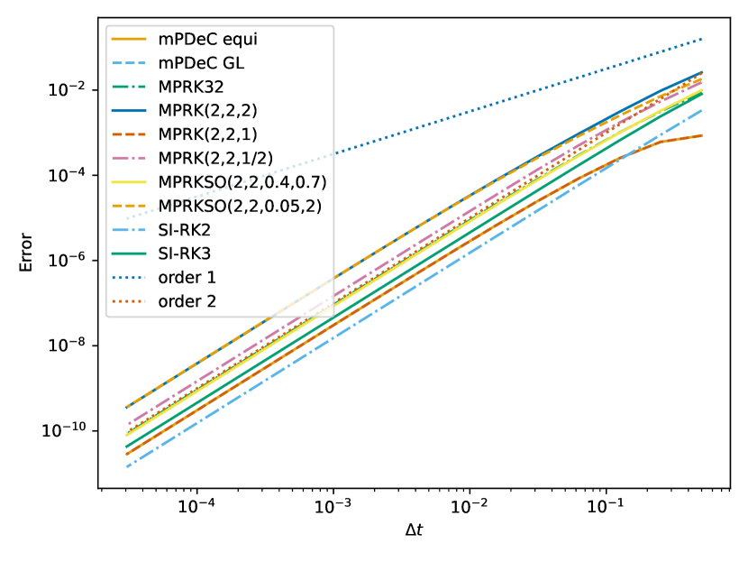
(a) Order 2 schemes, $\varepsilon=10^{-2}$

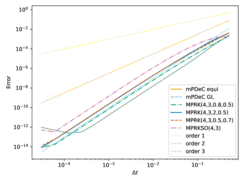
(b) Order 3 schemes, $\varepsilon=10^{-2}$

(c) Order 2 schemes, $\varepsilon=10^{-16}$

(d) Order 3 schemes, $\varepsilon=10^{-16}$

(e) Order 2 schemes, $\varepsilon=10^{-250}$

(f) Order 3 schemes, $\varepsilon=10^{-250}$

Figure 2: Error decay for the system (12) with $\theta=0.5$, at time $T=1$ with second and third order methods and different $\varepsilon$.

(a) Order 4 schemes, $\varepsilon=10^{-2}$

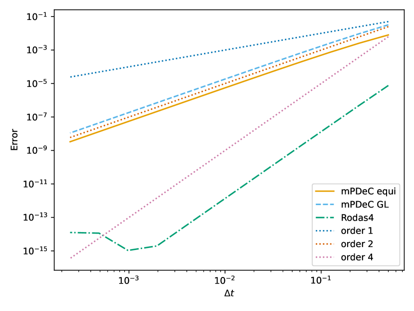
(b) Order 4 schemes, $\varepsilon=10^{-16}$

Figure 3: Error decay for the system (12) with $\theta=0.5$, at time $T=1$ with fourth order methods and different $\varepsilon$.

The fall back to first and second order is due to an error in the first time steps when one initial condition is close to 0. As soon as this component becomes large enough the error goes back to the expected one. This leaves either a shift of some $\Delta t$ on the solution or a first time step with a second order error. To grasp why we lose order of accuracy, we need to understand what happens in the limit of our schemes for $\varepsilon\to 0$ for the first time step. We remark that, in the linear system case, $\tilde{p}_{ij}$ and $\tilde{d}_{ij}$ defined in Theorem 1.2 as $\tilde{d}_{ij}(u)=d_{ij}(u)/u_{i}$ and $\tilde{p}_{ij}(u)=p_{ij}(u)/u_{j}$ are positive and constant. As an example, we can see the role of these production/destruction rates in the MPE

$$u^{1}_{i}=u^{0}_{i}+\Delta t\sum_{j}\left(\tilde{p}_{ij}(u^{0})\cancel{u_{j}^{0}}\frac{u^{1}_{j}}{\cancel{u_{j}^{0}}}-\tilde{d}_{ij}(u^{0})\cancel{u_{i}^{0}}\frac{u^{1}_{i}}{\cancel{u_{i}^{0}}}\right),$$ (42)

$$u^{1}_{i}=\frac{u^{0}_{i}+\Delta t\sum_{j}\tilde{p}_{ij}(u^{0})u^{1}_{j}}{1+\Delta t\sum_{j}\tilde{d}_{ij}(u^{0})}=u^{0}_{i}+\Delta t\sum_{j\in I}\left(\tilde{p}_{ij}(u^{0})u_{j}^{1}-\tilde{d}_{ij}(u^{0})u_{i}^{0}\right)+\mathcal{O}(\Delta t^{2}).$$ (43)

Hence, we see that the method that we obtain for vanishing initial condition $\varepsilon\to 0$ is well defined and, in this case, leads to a consistent and first order scheme.

This is not true for MPRK(2,2,$\alpha$) for all $\alpha$. The first stage of the scheme is a MPE step and it does not introduce issues. The second stage depends on the coefficient $\alpha$. Let us define $\omega=\frac{1}{2\alpha}$, the second stage reads

$$u_{i}^{1}=u_{i}^{0}+\Delta t\sum_{j}\left[\left(\frac{(1-\omega)p_{ij}(y^{1})+\omega p_{ij}(y^{2})}{(y^{2}_{j})^{1/\alpha}(y^{1}_{j})^{1-1/\alpha}}\right)u^{1}_{j}-\left(\frac{(1-\omega)d_{ij}(y^{1})+\omega d_{ij}(y^{2})}{(y^{2}_{i})^{1/\alpha}(y^{1}_{i})^{1-1/\alpha}}\right)u^{1}_{i}\right].$$ (44)

Here, we cannot simplify as before the linear terms of destructions and productions. If we focus on the destruction term for the vanishing constituent, i.e., $u_{i}^{0}=\varepsilon=y^{1}_{i}\to 0$, and if we suppose that the first step is such that $y^{2}_{i}\geq C_{2}\Delta t$, this is true as we have seen in the MPE step, we have that

$$\lim_{y^{1}_{i}\to 0}\frac{(1-\omega)d_{ij}(y^{1})+\omega d_{ij}(y^{2})}{(y^{2}_{i})^{1/\alpha}(y^{1}_{i})^{1-1/\alpha}}=\begin{cases}0,&\text{if }1-1/\alpha<0\Leftrightarrow\alpha<1,\\ \omega\tilde{d}_{ij}(y^{2}),&\text{if }1-1/\alpha=0\Leftrightarrow\alpha=1,\\ \infty,&\text{if }1-1/\alpha>0\Leftrightarrow\alpha>1,\end{cases}$$ (45)

where $\tilde{d}_{ij}$ is defined in Theorem 1.2.

Hence, for $\alpha>1$, when collecting the term $u_{i}^{1}$ on the left–hand side, we have that $\lim_{\varepsilon\to 0}u_{i}^{1}=0$. This is a zero-th order error step. Nevertheless, as one can see also in Figure 2 and Figure 1(b), after some steps the regime $u_{2}\ll\Delta t$ is abandoned and the classical accuracy is restored, leading to an error of the order of $\mathcal{O}(\Delta t)$ at a final time $T$.

For $\alpha<1$ we have that the contribution of the destruction terms to this equation tends to 0 as $\varepsilon\to 0$, while they where expected to give, for (12), a contribution of the order of $\Delta t$ (as $d_{21}(y^{1})=(1-\theta)y^{1}_{2}=\mathcal{O}(\Delta t)$). This leads to an error of $\mathcal{O}(\Delta t^{2})$ for the first time step, i.e., a first order error. At the second step the regime $u_{2}\ll\Delta t$ is already left, hence, the formal second order of accuracy is then restored. So, at a final time we have an error of $\mathcal{O}(\Delta t^{2})+\mathcal{O}(\Delta t^{2})=\mathcal{O}(\Delta t^{2})$. Even if in this case we do not observe an order reduction at a final time, the first time step shows order reduction and this is very common also in other higher order methods and this type of reduction would lead to a $\mathcal{O}(\Delta t^{2})$ at the final time.

Finally, for $\alpha=1$ none of these behaviors happen, no order reduction is observed and an error of $\mathcal{O}(\Delta t^{3})$ is formally obtained at the first time step.

We can generalize the two problematic cases that we have just explained into two lemmas. These configurations are common to many MP schemes. Hence, it will be easy then to recast each scheme to one of these cases. For the mPDeC schemes a similar issue arises from the negative coefficients and it will be discussed later.

In general, to obtain a certain order of accuracy, the RK methods build stages of increasing order of accuracy, so that the final step can perform a linear combination of functions of enough accurate stages. If the expected order of accuracy is lost in any of these stages, we might have an order reduction in that timestep update. This is why we need to study all the stages of the MP schemes to check in which of those there is an order reduction and up to which order this happens. This will lead to the understanding of the final order reduction of the method. In the following, we study a general stage and how the order reduction can happen and, then, we check which MPRK is affected in which stage by this behavior.

First of all, let us write a general step of an MPRK scheme for the second component of the ODE (12) at a certain stage $s$, exploiting the conservation property, as

$$y_{2}^{s}=u_{2}^{0}+\Delta t\sum_{j<s}\gamma_{j}^{s}\left(p_{21}(y^{j})\frac{y_{1}^{s}}{\sigma_{1}^{j}}-d_{21}(y^{j})\frac{y_{2}^{s}}{\sigma_{2}^{j}}\right)=u_{2}^{0}+\Delta t\sum_{j<s}\gamma_{j}^{s}\left(\theta\frac{y^{j}_{1}}{\sigma_{1}^{j}}(1-y_{2}^{s})-(1-\theta)\frac{y^{j}_{2}}{\sigma_{2}^{j}}y_{2}^{s}\right),$$ (46)

with $\gamma_{j}^{s}$ some nonnegative RK coefficients and $\sigma_{i}^{j}$ the different denominator of the various MPRK schemes. Now, the troubles come when there are some $\sigma_{2}^{j}$ that are an $\mathcal{O}(\varepsilon)$ or when $1/\sigma_{2}^{j}=\mathcal{O}(\varepsilon)$ and they do not match the destruction terms. These cases correspond to what observed in MPRK(2,2,$\alpha$) for $\alpha>1$ and $\alpha<1$ respectively, while it is not the case of MPE where cancellation leads to a consistent approximation. To be more general, let us consider $\sigma_{2}^{j}=\mathcal{O}(\eta)$ or $1/\sigma_{2}^{j}=\mathcal{O}(\eta)$, where $\eta$ can be a power of $\varepsilon$ or a ratio between $\varepsilon$ and $\Delta t$. As an example, you can refer to the MPRK(2,2,$\alpha$), where at the last stage the denominator is $\sigma_{2}^{1}=\sigma_{2}^{2}=(y_{2}^{2})^{1/\alpha}(y_{2}^{1})^{1-1/\alpha}=\mathcal{O}(\Delta t^{1/\alpha}\varepsilon^{1-1/\alpha})$. This will be the case in many situations. It will be useful to use the Big Theta Landau symbol $f(x)=\Theta(g(x))$ to indicate that

$$0<\liminf_{x\to 0}\frac{|f(x)|}{g(x)}\leq\limsup_{x\to 0}\frac{|f(x)|}{g(x)}<\infty.$$

First, we study the case where $\sigma^{j}_{2}=\Theta(\eta)$ which corresponds to the MPRK(2,2,$\alpha$) for $\alpha>1$.

Lemma 5.2.

Consider the problem (12) with $0<\theta<1$ and initial condition $(1-\varepsilon,\varepsilon)$ with $0<\varepsilon$. Consider the update step at the first time step given by (46). Suppose there is an $\ell<s$ with $\gamma_{\ell}^{s}>0$ such that $\sigma_{2}^{\ell}=\Theta(\eta)$, $y_{2}^{\ell}=\Theta(\Delta t)$ and consider the limit for $\Delta t\to 0$, $\frac{\eta}{\Delta t^{2}}\to 0$ and $\frac{\varepsilon}{\Delta t}\to 0$. Moreover, suppose that for all stages $j$: $\frac{y_{2}^{j}}{\sigma_{2}^{j}}=\mathcal{O}\left(\frac{y_{2}^{\ell}}{\sigma_{2}^{\ell}}\right)$. Then,

$$y_{2}^{s}=\Theta\left(\frac{\eta}{\Delta t}\right)=u_{2}^{ex}+\Theta(\Delta t),$$

where $u_{2}^{ex}$ is the exact solution after the first time step.

Proof.

First of all, let us observe that $\frac{\eta}{\Delta t}=\frac{\eta}{\Delta t^{2}}\Delta t\to 0$ as both $\frac{\eta}{\Delta t}\to 0$ and $\Delta t\to 0$. From (46) we can write the definition of $y_{2}^{s}$ as

$$\Bigg{[}1+\underbrace{\Delta t\sum_{j<s}\gamma_{j}^{s}\theta\frac{y_{1}^{j}}{\sigma_{1}^{j}}}_{\Theta(\Delta t)}+\underbrace{\Delta t\sum_{j<s}\gamma_{j}^{s}(1-\theta)\frac{y_{2}^{j}}{\sigma_{2}^{j}}}_{\Theta(\frac{\Delta t^{2}}{\eta})}\Bigg{]}y_{2}^{s}=\underbrace{y_{2}^{0}}_{=\varepsilon}+\underbrace{\Delta t\sum_{j<s}\gamma_{j}^{s}\theta\frac{y_{1}^{j}}{\sigma_{1}^{j}}}_{\Theta(\Delta t)}.$$ (47)

The scaling indicated by Landau symbols can be explained from hypotheses, using also $y_{1}=\mathcal{O}(1)$ for all stages and consequently $\sigma_{1}=\mathcal{O}(1)$; the initial value is $y_{2}^{0}=\varepsilon$ and all the coefficients are constant. Then, the dominating term on the left-hand side is the $\Theta(\frac{\Delta t^{2}}{\eta})$, the only one going to infinity, and on the right side it is the $\Theta(\Delta t)$ as $\frac{\varepsilon}{\Delta t}\to 0$. So, we can write that

$$y_{2}^{s}= \frac{\varepsilon+\Delta t\displaystyle\sum_{j<s}\gamma_{j}^{s}\theta\frac{y_{1}^{j}}{\sigma_{1}^{j}}}{1+\Delta t\displaystyle\sum_{j<s}\gamma_{j}^{s}\theta\frac{y_{1}^{j}}{\sigma_{1}^{j}}+\Delta t\displaystyle\sum_{j<s}\gamma_{j}^{s}(1-\theta)\frac{y_{2}^{j}}{\sigma_{2}^{j}}}=\frac{\frac{\eta}{\Delta t^{2}}\varepsilon+\frac{\eta}{\Delta t}\displaystyle\sum_{j<s}\gamma_{j}^{s}\theta\frac{y_{1}^{j}}{\sigma_{1}^{j}}}{\frac{\eta}{\Delta t^{2}}+\underbrace{\frac{\eta}{\Delta t}\displaystyle\sum_{j<s}\gamma_{j}^{s}\theta\frac{y_{1}^{j}}{\sigma_{1}^{j}}}_{\Theta(\frac{\eta}{\Delta t})}+\underbrace{\frac{\eta}{\Delta t}\displaystyle\sum_{j<s}\gamma_{j}^{s}(1-\theta)\frac{y_{2}^{j}}{\sigma_{2}^{j}}}_{\Theta(1)}}$$ (48)

$$= \frac{\frac{\eta}{\Delta t}\displaystyle\sum_{j<s}\gamma_{j}^{s}\theta\frac{y_{1}^{j}}{\sigma_{1}^{j}}}{\frac{\eta}{\Delta t}\displaystyle\sum_{j<s}\gamma_{j}^{s}(1-\theta)\frac{y_{2}^{j}}{\sigma_{2}^{j}}}+\Theta(1)\!\!\left(\frac{\eta\varepsilon}{\Delta t^{2}}\!-\!\frac{\eta}{\Delta t^{2}}\frac{\eta}{\Delta t}\displaystyle\sum_{j<s}\gamma_{j}^{s}\theta\frac{y_{1}^{j}}{\sigma_{1}^{j}}\!-\!\frac{\eta^{2}}{\Delta t^{2}}\left(\displaystyle\sum_{j<s}\gamma_{j}^{s}\theta\frac{y_{1}^{j}}{\sigma_{1}^{j}}\right)^{2}\right)\!\!+\dots$$ (49)

$$= \frac{\displaystyle\sum_{j<s}\gamma_{j}^{s}\theta\frac{y_{1}^{j}}{\sigma_{1}^{j}}}{\displaystyle\sum_{j<s}\gamma_{j}^{s}(1-\theta)\frac{y_{2}^{j}}{\sigma_{2}^{j}}}+\mathcal{O}\left(\frac{\eta}{\Delta t}\frac{\varepsilon}{\Delta t}\right)+\mathcal{O}\left(\frac{\eta}{\Delta t}\frac{\eta}{\Delta t^{2}}\right)+\mathcal{O}\left(\frac{\eta}{\Delta t}\frac{\eta}{\Delta t}\right)=\Theta\left(\frac{\eta}{\Delta t}\right).$$ (50)

To obtain the previous formula is convenient to multiply numerator and denominator of $y_{2}^{s}$ by $\sigma_{2}^{\ell}$ and then, after having simplified $\Delta t$, at the numerator there is a $\Theta(1)$ and at the denominator the term $\frac{y_{2}^{\ell}}{\sigma_{2}^{\ell}}$ dominates the sum. ∎

This lemma shows that in the stages where the hypotheses are verified we obtain a 0-th order accurate update. Still, the value of $y_{2}^{j}=\Theta\left(\frac{\eta}{\Delta t}\right)$ and it is larger than $\eta$ (for small $\Delta t$). So, if this operation is repeated and we consider the result after a time step as a new initial condition, the new initial value $\varepsilon$ will keep increasing (and consequently $\eta$ which is proportional to $\varepsilon$), the regime $y_{2}\ll\Delta t$ is abandoned after some time steps and the classical accuracy is restored for following time steps. Usually, in these cases an error of $\mathcal{O}(\Delta t)$ at a final step is observed, as a first order method.

The second situation we encounter is the opposite, when the exponents of the schemes are such that $1/\sigma_{2}^{j}$ is an $\mathcal{O}(\varepsilon)$ or one of its powers, as for MPRK(2,2,$\alpha$) for $\alpha<1$.

Lemma 5.3.

Consider the problem (12) with $0<\theta<1$ and initial condition $(1-\varepsilon,\varepsilon)$ with $0<\varepsilon$. Consider the update step at the first time step given by (46). Suppose that exists $\ell<s$ with $\gamma_{\ell}^{s}>0$ such that $1/\sigma_{2}^{\ell}=\Theta(\eta)$ and $y_{2}^{\ell}=\Theta(\Delta t)$ and consider the limit for $\Delta t\to 0$, $\frac{\eta}{\Delta t}\to 0$ and $\frac{\varepsilon}{\Delta t}\to 0$. Moreover, suppose that for all $j<s$, $\frac{y_{2}^{j}}{\sigma_{2}^{j}}=\mathcal{O}(1)$. Then, $y_{2}^{s}$ is at most an approximation of order 1 of the exact solution and the error is an $\mathcal{O}(\Delta t^{2}).$

Proof.

First we prove that $y^{s}_{2}=\Theta(\Delta t)$ and afterwards, we show that it cannot be a second order approximation. From (47) it follows that

$$\Bigg{[}1+\underbrace{\Delta t\sum_{j<s}\gamma_{j}^{s}\theta\frac{y_{1}^{j}}{\sigma_{1}^{j}}}_{\Theta(\Delta t)}+\underbrace{\Delta t\sum_{j<s}\gamma_{j}^{s}(1-\theta)\frac{y_{2}^{j}}{\sigma_{2}^{j}}}_{\mathcal{O}(\Delta t)}\Bigg{]}y_{2}^{s}=\underbrace{y_{2}^{0}}_{=\varepsilon}+\underbrace{\Delta t\sum_{j<s}\gamma_{j}^{s}\theta\frac{y_{1}^{j}}{\sigma_{1}^{j}}}_{\Theta(\Delta t)},$$ (51)

so that the dominant term on the LHS is 1 and on the RHS is the $\Theta(\Delta t)$. Hence, we obtain

$$y_{2}^{s}=\Delta t\sum_{j<s}\gamma_{j}^{s}\theta\frac{y_{1}^{j}}{\sigma_{1}^{j}}+\mathcal{O}(\varepsilon)+\mathcal{O}(\Delta t^{2})=\Theta(\Delta t).$$ (52)

Consider again the update equation (46) and supposed that it is of order of accuracy $p>1$ in the nonvanishing initial condition regime. We see that

$$y_{2}^{s} =u_{2}^{0}+\Delta t\sum_{j<s}\gamma_{j}^{s}p_{21}(y^{j})\frac{y_{1}^{s}}{\sigma_{1}^{j}}-\Delta t\sum_{j<s}\gamma_{j}^{s}d_{21}(y^{j})\frac{y_{2}^{s}}{\sigma_{2}^{j}}$$ (53)

$$=u_{2}^{0}+\Delta t\sum_{j<s}\gamma_{j}^{s}p_{21}(y^{j})-\Delta t\sum_{j\neq\ell}\gamma_{j}^{s}d_{21}(y^{j})\frac{y_{2}^{s}}{\sigma_{2}^{j}}-\Delta t\gamma_{\ell}^{s}d_{21}(y^{\ell})\frac{y_{2}^{s}}{\sigma_{2}^{\ell}},$$ (54)

Focusing on the last term we observe that

$$\Delta t\gamma_{\ell}^{s}d_{21}(y^{\ell})\frac{y_{2}^{s}}{\sigma_{2}^{\ell}}=\Delta t\gamma_{\ell}^{s}\theta y^{\ell}_{2}\frac{y_{2}^{s}}{\sigma_{2}^{\ell}}=\Delta t\gamma_{\ell}^{s}\theta\underbrace{\frac{y^{\ell}_{2}}{\sigma_{2}^{\ell}}}_{\Theta(\eta\Delta t)}\underbrace{y_{2}^{s}}_{\Theta(\Delta t)}=\Theta(\Delta t^{3}\eta),$$ (55)

while for the unweighted term of the original highly accurate RK method we have

$$\Delta t\gamma_{\ell}^{s}d_{21}(y^{\ell})=\Theta(\Delta t^{2}),$$ (56)

hence, the difference of the two is $\Theta(\Delta t^{2})$. Hence, the destruction term contribution related to stage $\ell$ is approximated with an error of $\Theta(\Delta t^{2})$. So that the error for the stage $s$ is affected mainly by this error, i.e.,

$$y_{2}^{s}=y_{2}^{ex}+\Theta(\Delta t^{2}).$$ (57)

∎

This proof shows that when a scheme falls in the hypotheses of this lemma, we have a first step with only accuracy order of 1, but, immediately after, the value of $u_{2}$ is far away from zero and the classical order of accuracy is restored. Then, at a final time the error will be a $\Theta(\Delta t^{2})$. We remark that the hypothesis $\frac{y_{2}^{j}}{\sigma_{2}^{j}}=\mathcal{O}(1)$ is not restrictive as it discriminates the first lemma case and second lemma case. Indeed, when this hypothesis is not fulfilled, there exists an $\ell$ such that $\sigma_{2}^{\ell}=o(y_{2}^{\ell})$, and by an opportune definition of $\eta$ such that $\sigma_{\ell}^{2}=\Theta(\eta)$ fulfills the hypotheses of Lemma 5.2.

Now we can use these results to show the accuracy of all the modified Patankar schemes with positive Runge–Kutta coefficients.

Theorem 5.4 (Accuracy of Patankar schemes with nonnegative RK coefficients for vanishing initial data).

Consider the system of ODEs (12) with $u_{0}=(1-\varepsilon,\varepsilon)$ with vanishing initial condition, i.e., $\frac{\varepsilon}{\Delta t^{r}}\to 0$ as $\Delta t\to 0$ with $r$ large enough depending on the scheme so that hypotheses of previous lemmas are met. Then, the modified Patankar schemes with positive coefficients have errors in the first time steps and at a final time as shown in Table 2 (for mPDeC we refer to Theorem 5.5).

Method	Parameters	First time step error	Final time error
MPRK(2,2,$\alpha$)	$\alpha=1$	$\Theta(\Delta t^{3})$	$\Theta(\Delta t^{2})$
MPRK(2,2,$\alpha$)	$\alpha>1$	$\Theta(\Delta t)$	$\Theta(\Delta t)$
MPRK(2,2,$\alpha$)	$\frac{1}{2}\leq\alpha<1$	$\Theta(\Delta t^{2})$	$\Theta(\Delta t^{2})$
MPRK(4,3,$\alpha,\beta$)	$q>1$	$\Theta(\Delta t)$	$\Theta(\Delta t)$
MPRK(4,3,$\alpha,\beta$)	$p>1$ and $q\leq 1$	$\Theta(\Delta t^{2})$	$\Theta(\Delta t^{2})$
MPRK(4,3,$\alpha,\beta$)	$p\leq 1$ and $q\leq 1$ and $pq\neq 1$	$\Theta(\Delta t^{3})$	$\Theta(\Delta t^{3})$
MPRK(4,3,$\alpha,\beta$)	$p=q=1$	$\Theta(\Delta t^{4})$	$\Theta(\Delta t^{3})$
MPRKSO(2,2,$\alpha$,$\beta$)	$\gamma<1$	$\Theta(\Delta t)$	$\Theta(\Delta t)$
MPRKSO(2,2,$\alpha$,$\beta$)	$\gamma=1$	$\Theta(\Delta t^{3})$	$\Theta(\Delta t^{2})$
MPRKSO(2,2,$\alpha$,$\beta$)	$\gamma>1$	$\Theta(\Delta t^{2})$	$\Theta(\Delta t^{2})$
MPRKSO(4,3)		$\Theta(\Delta t^{2})$	$\Theta(\Delta t^{2})$
MPRK(3,2)		$\Theta(\Delta t^{3})$	$\Theta(\Delta t^{2})$
SI-RK2		$\Theta(\Delta t^{3})$	$\Theta(\Delta t^{2})$
SI-RK3		$\Theta(\Delta t^{3})$	$\Theta(\Delta t^{2})$
mPDeC	Equispaced, nonnegative $\theta^{M}_{j}$	$\Theta(\Delta t^{2})$	$\Theta(\Delta t^{2})$
mPDeC	Equispaced, negative $\theta^{M}_{j}$	$\Theta(\Delta t)$	$\Theta(\Delta t)$
mPDeC	Gauss-Lobatto any order	$\Theta(\Delta t^{2})$	$\Theta(\Delta t^{2})$

Table 2: Accuracy of Patankar methods for vanishing initial conditions with parameters defined at the definition of each scheme, see MPRK(2,2,$\alpha$), MPRK(4,3,$\alpha,\beta$), MPRKSO(2,2,$\alpha$,$\beta$) and mPDeC

Proof.

We analyze all the methods stage by stage.

• Let us start with MPRK(2,2,$\alpha$). The first stage is an MPE step, which coincides with an implicit–Euler step for this problem and gives that $y_{2}^{2}=u_{2}(\alpha\Delta t)+\mathcal{O}(\Delta t^{2})=\Theta(\Delta t)$ for all parameters. In the last stage, we have that the critical factor is $\sigma_{2}^{2}=(y_{2}^{2})^{1/\alpha}(y_{2}^{1})^{1-1/\alpha}=\Theta(\Delta t^{1/\alpha}(\varepsilon)^{1-1/\alpha})$ at the denominator, while $y_{2}^{2}=\Theta(\Delta t)$ being at the numerator.

  • When $\alpha=1$, then $\sigma_{2}^{2}=\Theta(\Delta t)$ and this does not arise problems, hence the classical accuracy is restored and we have an error of $\mathcal{O}(\Delta t^{3})$ for the first time step.

  • For $\alpha>1$ we have that $1-1/\alpha>0$ and Lemma 5.2 applies with $\eta=\varepsilon^{1-1/\alpha}\Delta t^{1/\alpha}$ when

    $$\frac{\eta}{\Delta t^{2}}=\varepsilon^{1-1/\alpha}\Delta t^{1/\alpha-2}\to 0\text{ and }\frac{\varepsilon}{\Delta t}\to 0$$

    as $\Delta t\to 0$. Hence, $u^{1}_{2}=\Theta\left(\left(\frac{\varepsilon}{\Delta t}\right)^{1-1/\alpha}\right)=u_{2}(t^{1})+\Theta(\Delta t)$. It must be noticed that $\varepsilon=o\left(\left(\frac{\varepsilon}{\Delta t}\right)^{1-1/\alpha}\right)$, hence, each time step is moving away from the region $u_{2}^{n}\ll\Delta t$. After a certain number of time steps the regime $\eta\ll\Delta t$ will be lost and classical accuracy will be restored. The first errors of $\Theta(\Delta t)$ will dominate the final error.

  • For $\frac{1}{2}\leq\alpha<1$ we have that $-1\leq 1-1/\alpha<0$ and Lemma 5.3 applies with $\eta=\Theta(\Delta t^{1/\alpha}\varepsilon^{1/\alpha-1})$ when $\frac{\eta}{\Delta t}=\varepsilon^{1/\alpha-1}\Delta t^{1/\alpha-1}\to 0$ as $\Delta t\to 0$. This means that for the first time step it holds that $u^{1}_{2}=u_{2}^{ex}+\Theta(\Delta t^{2})=\Theta(\Delta t)$. So, from the second time step classical error $\mathcal{O}(\Delta t^{3})$ accumulates at each time step, leading to an error of $\mathcal{O}(\Delta t^{2})$ at a final time.

• MPRK(4,3,$\alpha,\beta$) has a first stage of MPE, so $y^{2}_{2}=y_{2}^{ex}(\alpha\Delta t)+\mathcal{O}(\Delta t^{2})=\Theta(\Delta t)$. Again, according to $p$ and $q$, exactly as for the MPRK(2,2,$\alpha$) we have three situations.

  $$\begin{cases}y_{2}^{3}=y_{2}(\beta\Delta t)+\mathcal{O}(\Delta t^{3})=\Theta(\Delta t),&p=1,\\ y_{2}^{3}=y_{2}(\beta\Delta t)+\mathcal{O}(\Delta t^{2})=\Theta(\Delta t),&p<1,\\ y_{2}^{3}=y_{2}(\beta\Delta t)+\mathcal{O}(\Delta t)=\Theta\left(\left(\frac{\varepsilon}{\Delta t}\right)^{1-1/p}\right),&p>1,\end{cases}$$ (58)

  and

  $$\begin{cases}\sigma_{2}=y_{2}(\Delta t)+\mathcal{O}(\Delta t^{3})=\Theta(\Delta t),&q=1,\\ \sigma_{2}=y_{2}(\Delta t)+\mathcal{O}(\Delta t^{2})=\Theta(\Delta t),&q<1,\\ \sigma_{2}=y_{2}(\Delta t)+\mathcal{O}(\Delta t)=\Theta\left(\left(\frac{\varepsilon}{\Delta t}\right)^{1-1/p}\right),&q>1.\end{cases}$$ (59)

  These are obtained with the previous lemmas exactly as in the case of MPRK(2,2,$\alpha$).

  • Now, if $q>1$ and $\sigma_{2}=\Theta\left(\left(\frac{\varepsilon}{\Delta t}\right)^{1-1/q}\right)$ and it verifies the hypotheses of Lemma 5.2, i.e. $\varepsilon^{1-1/q}\Delta t^{1/q-2}\to 0$ and $\frac{\varepsilon}{\Delta t}\to 0$ as $\Delta t\to 0$, then, for Lemma 5.2, we have that $u_{2}^{1}=\Theta\left(\frac{\varepsilon^{1-1/q}}{\Delta t^{2-1/q}}\right)$. This means that at the first time step we have an error of $\Theta(\Delta t)$. Again, we see that $\varepsilon=o\left(\frac{\varepsilon^{1-1/q}}{\Delta t^{2-1/q}}\right)$ and this means that only few time steps will verify the hypotheses of Lemma 5.3. Afterwards, the original third order accuracy will be restored, leading to an overall error of $\mathcal{O}(\Delta t)$ at a final time.

  • If $q<1$ then $\sigma_{2}=u_{2}(\Delta t)+\mathcal{O}(\Delta t^{2})$ for Lemma 5.3 with $\eta=\Delta t^{1/q}\varepsilon^{1-1/q}$ when $(\Delta t\varepsilon)^{1/q-1}\to 0$ and $\frac{\varepsilon}{\Delta t}\to 0$ for $\Delta t\to 0$. Then, $\frac{u_{2}(t^{1})}{\sigma_{2}}=1+\Theta(\Delta t^{2})$ which leads to an error of $\Theta(\Delta t^{3})$ at the first time step.

  • If $q=1$ none of the lemmata apply and the weighting factor should be of the expected third order accuracy.

  • If $p>1$ then $y_{2}^{3}=u_{2}(\beta\Delta t)+\Theta(\Delta t)$ for Lemma 5.3 when $\varepsilon^{1-1/p}\Delta t^{1/p-2}\to 0$ and $\frac{\varepsilon}{\Delta t}\to 0$ as $\Delta t\to 0$, hence this brings in the production and destruction terms of the final update an error of $\Theta(\Delta t^{2})$.

  • If $p<1$ then $y_{2}^{3}=u_{2}(\beta\Delta t)+\Theta(\Delta t^{2})$ for Lemma 5.3 when $\frac{\varepsilon}{\Delta t}\to 0$, which brings in the final update an error of $\Theta(\Delta t^{3})$.

  • If $p=1$ this would not contribute to errors larger than the accuracy order of the scheme.

  Putting all the information together we obtain the errors in Table 2, recalling that, except for $q>1$, only the first time step falls in the hypotheses of the lemmas, so, it is the only time step affected by these errors, while for $q>1$ some time steps will be effected. Anyway, the error at the final solution is bounded by the third order accuracy of the scheme itself.

• For MPRKSO(2,2,$\alpha$,$\beta$) the same arguments of MPRK(2,2,$\alpha$) apply with $\gamma$ in place of $\alpha$.

• For MPRKSO(4,3) we have that the first stage is again an MPE step and $y_{2}^{1}=\Theta(\Delta t)$. Then, $1/\varrho_{2}=\Theta(\frac{\varepsilon}{\Delta t^{2}})$. For the equation of $y_{2}^{3}$ Lemma 5.3 applies with $\eta=\frac{\varepsilon}{\Delta t^{2}}$ when $\frac{\eta}{\Delta t}=\frac{\varepsilon}{\Delta t^{3}}\to 0$ as $\Delta t\to 0$, hence $y_{2}^{3}=u_{2}((\alpha_{20}+\alpha_{21})\Delta t)+\Theta(\Delta t^{2}).$ Then, $\mu_{2}=\Theta\left(\frac{\Delta t^{s}}{\varepsilon^{s-1}}\right)$ which makes the equation for $\tilde{a}_{2}$ fall in the hypotheses of Lemma 5.3 with $\eta=\frac{\varepsilon^{s-1}}{\Delta t^{s}}$ when $\frac{\eta}{\Delta t}=\frac{\varepsilon^{s-1}}{\Delta t^{s+1}}\to 0$ as $\Delta t\to 0$. Hence, $\tilde{a}_{2}=u_{2}((\eta_{1}+\eta_{2})\Delta t)+\Theta(\Delta t^{2}).$ Then, $\sigma_{2}=\tilde{a}_{2}+\Theta(\frac{\varepsilon^{2}}{\Delta t^{2}})=u_{2}(\Delta t)+\Theta(\Delta t)$. This means that $\frac{u_{2}(\Delta t)}{\sigma_{2}}=1+\Theta(\Delta t)$, which sums up to a first order error $\Theta(\Delta t^{2})$ for the first step. From the second step on, the third order accuracy is restored. Hence, at a final time an error of a $\Theta(\Delta t^{2})$ is observable.

• In MPRK(3,2) the first stage exploits the cancellation between the destruction and production of the same constituents as for all the MPE steps. All the other stages never present $y_{2}^{1}$ at the denominator of the MP weights, hence, none of the cases of the previous lemmas is met. So no order reduction phenomena appear.

• In SI-RK2 and SI-RK3 the cancellation $d_{21}(y)/y_{2}=(1-\theta)$ is always exploited, so there is no troubled term at the denominators. Hence, no order reduction is observed.

∎

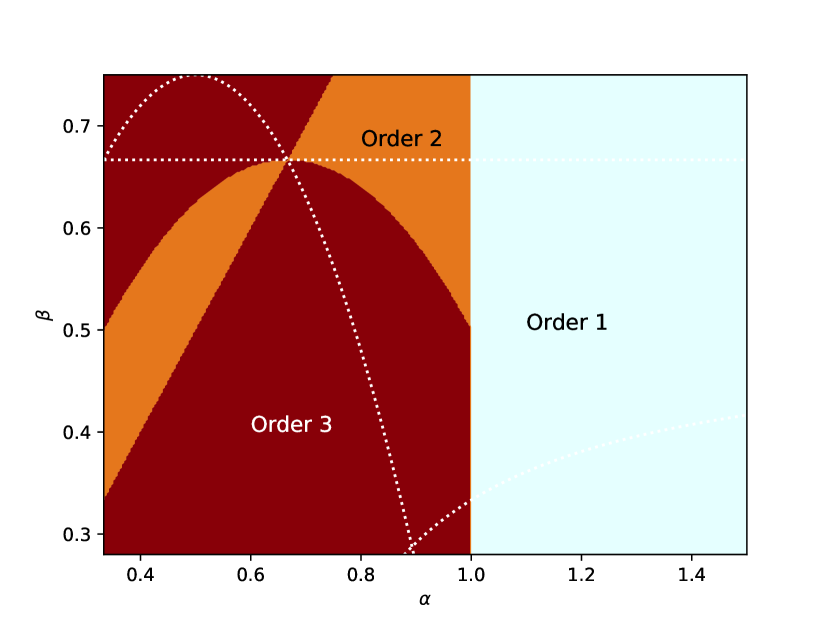
(a) MPRK(4,3,$\alpha,\beta$) orders: light blue first order, orange second order, brown third order

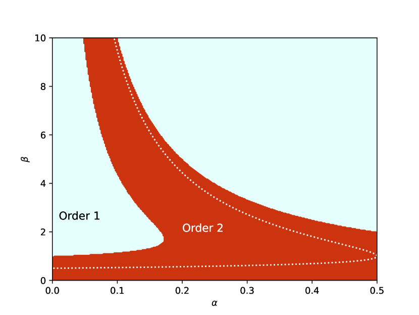
(b) MPRKSO(2,2,$\alpha$,$\beta$) orders: light blue first order, red second order

Figure 4: Order of accuracy of some schemes for vanishing initial conditions. The white dashed lines bound the positive RK coefficients area [28, 19].

As an example we want to focus on MPRK(3,4,2,0.5) plotted in Figure 2. For this scheme $p=3$ and $q=2$. To verify the hypotheses of the lemmata, we need to have $\frac{\varepsilon^{1-1/2}}{\Delta t^{2-1/2}}\to 0$ as $\Delta t\to 0$, which is equivalent to $\frac{\varepsilon}{\Delta t^{3}}\to 0$ as $\Delta t\to 0$. Indeed, in the simulation in Figure 2, we see that for $\Delta t\lesssim\varepsilon^{1/3}\approx 10^{-3.3}$ the error decays much faster than for $\Delta t\gtrsim 10^{-3}$.

In Figure 4(a) the order observable at a final time for MPRK(4,3,$\alpha,\beta$) is summarized, while in Figure 4(b) it is summarized for MPRKSO(2,2,$\alpha$,$\beta$). For the mPDeC the order reduction comes from the negative DeC coefficients in the update formulae. In the following theorem we described the order reduction for vanishing IC.

Theorem 5.5 (Loss of accuracy of mPDeC for vanishing initial data).

Consider the linear problem (12) with IC $(1-\varepsilon,\varepsilon)^{T}$. For vanishing IC, i.e., $\frac{\varepsilon}{\Delta t}\to 0$ as $\Delta t\to 0$, the mPDeC is of order 2 if $\exists\theta^{m}_{r}<0$ with $m\in[\![1,M-1]\!]=\{1,\dots,M-1\}$. If $\exists\theta^{M}_{r}<0$ the method is of order 1.

To prove the theorem let us introduce an useful proposition.

Proposition 5.6 (Carry over of the vanishing state).

Consider the linear problem (12) with IC $y^{0}=(1-\varepsilon,\varepsilon)^{T}$. If $\exists\theta^{m}_{r}<0$ with $m\geq 1$ and if $y_{2}^{(k-1),m}=\Theta(\varepsilon)$ with $\frac{\varepsilon}{\Delta t}\to 0$ as $\Delta t\to 0$, then $y_{2}^{(k),m}=\Theta(\varepsilon)$.

Proof.

Let us define $\theta^{m}_{-}$ the set of the negative coefficients among the $\theta^{m}_{r}$ and $\theta^{m}_{+}$ the set of the positive ones. We know that both sets are not empty, by hypothesis and by definition of $\theta_{r}^{m}$.

$$\begin{split}y_{i}^{m,(k)}-y^{0}_{i}&-\sum_{l\in\theta^{m}_{+}}\theta_{l}^{m}\Delta t\sum_{j}\left(p_{ij}(y^{l,(k-1)})\frac{y^{m,(k)}_{j}}{y_{j}^{m,(k-1)}}-d_{ij}(y^{l,(k-1)})\frac{y^{m,(k)}_{i}}{y_{i}^{m,(k-1)}}\right)\\ &-\sum_{l\in\theta^{m}_{-}}\theta_{l}^{m}\Delta t\sum_{j}\left(p_{ij}(y^{l,(k-1)})\frac{y^{m,(k)}_{i}}{y_{i}^{m,(k-1)}}-d_{ij}(y^{l,(k-1)})\frac{y^{m,(k)}_{j}}{y_{j}^{m,(k-1)}}\right)=0,\end{split}$$ (60)

$$\begin{split}y_{2}^{m,(k)}-\varepsilon&-\sum_{l\in\theta^{m}_{+}}\theta_{l}^{m}\Delta t\left(\theta{y^{l,(k-1)}_{1}}\frac{y^{m,(k)}_{1}}{y_{1}^{m,(k-1)}}-(1-\theta)y^{l,(k-1)}_{2}\frac{y^{m,(k)}_{2}}{y_{2}^{m,(k-1)}}\right)\\ &-\sum_{l\in\theta^{m}_{-}}\theta_{l}^{m}\Delta t\left(\theta{y^{l,(k-1)}_{1}}\frac{y^{m,(k)}_{2}}{y_{2}^{m,(k-1)}}-(1-\theta)y^{l,(k-1)}_{2}\frac{y^{m,(k)}_{1}}{y_{1}^{m,(k-1)}}\right)=0.\end{split}$$ (61)

We remind that for the conservation property of the scheme $y^{(k),r}_{1}=1-y^{(k),r}_{2}$. So, if we collect all the unknown terms in the left-hand side, we obtain

$$\begin{split}&\left[1+\Delta t\sum_{l\in\theta^{m}_{+}}\theta^{m}_{l}\left(\theta\frac{y^{l,(k-1)}_{1}}{y^{m,(k-1)}_{1}}+(1-\theta)\frac{y^{l,(k-1)}_{2}}{y^{m,(k-1)}_{2}}\right)-\Delta t\sum_{l\in\theta^{m}_{-}}\theta^{m}_{l}\left(\theta\frac{y^{l,(k-1)}_{1}}{y^{m,(k-1)}_{2}}+(1-\theta)\frac{y^{l,(k-1)}_{2}}{y^{m,(k-1)}_{1}}\right)\right]y_{2}^{m,(k)}\\ &=\varepsilon+\sum_{l\in\theta^{m}_{+}}\theta_{l}^{m}\Delta t\left(\theta\frac{y^{l,(k-1)}_{1}}{y_{1}^{m,(k-1)}}\right)-\sum_{l\in\theta^{m}_{-}}\theta_{l}^{m}\Delta t\left((1-\theta)\frac{y^{l,(k-1)}_{2}}{y_{1}^{m,(k-1)}}\right).\end{split}$$ (62)

Now, let us multiply the whole expression by the positive $y_{2}^{m,(k-1)}=\mathcal{O}(\varepsilon)$ and recalling that $y_{1}^{r,(k-1)}=1+\mathcal{O}(\Delta t)+\mathcal{O}(\varepsilon)$. We obtain

$$\begin{split}&\left[\mathcal{O}(\varepsilon)+\Delta t\sum_{l\in\theta^{m}_{+}}\theta^{m}_{l}(1-\theta){y^{l,(k-1)}_{2}}-\Delta t\sum_{l\in\theta^{m}_{-}}\theta^{m}_{l}\theta y^{l,(k-1)}_{1}\right]y_{2}^{m,(k)}\\ &=y^{m,(k-1)}_{2}\left(\varepsilon+\sum_{l\in\theta^{m}_{+}}\theta_{l}^{m}\Delta t\left(\theta\frac{y^{l,(k-1)}_{1}}{y_{1}^{m,(k-1)}}\right)-\sum_{l\in\theta^{m}_{-}}\theta_{l}^{m}\Delta t\left((1-\theta)\frac{y^{l,(k-1)}_{2}}{y_{1}^{m,(k-1)}}\right)\right).\end{split}$$ (63)

Now, the term $\Delta t\sum_{l\in\theta^{m}_{-}}\theta^{m}_{l}\left(\theta y^{l,(k-1)}_{1}\right)$ is the dominant in the left hand side, since $y_{2}^{l,(k-1)}=\mathcal{O}(\Delta t)$. Similarly the right hand side is dominated by the $y_{1}$ terms. Hence, we obtain

$$y^{m,(k)}_{2} =\frac{y_{2}^{m,(k-1)}\sum_{l\in\theta^{m}_{+}}\Delta t\theta_{l}^{m}\theta\frac{y_{1}^{l,(k-1)}}{y_{1}^{m,(k-1)}}+\mathcal{O}(\varepsilon^{2})+\mathcal{O}(\varepsilon\Delta t^{2})}{-\Delta t\sum_{l\in\theta^{m}_{-}}\theta^{m}_{l}\theta y_{1}^{l,(k-1)}+\mathcal{O}(\varepsilon)+\mathcal{O}(\Delta t^{2})}$$ (64)

$$=y_{2}^{m,(k-1)}\frac{\sum_{l\in\theta^{m}_{+}}\theta_{l}^{m}\frac{y_{1}^{l,(k-1)}}{y_{1}^{m,(k-1)}}}{-\sum_{l\in\theta^{m}_{-}}\theta^{m}_{l}y_{1}^{l,(k-1)}}+\mathcal{O}(\varepsilon^{2})+\mathcal{O}(\varepsilon\Delta t^{2})=\Theta(\varepsilon),$$ (65)

because all $y_{1}^{l,(k-1)}$ are $\mathcal{O}(1)$. Hence, the proposition is proven. ∎

The proof of the theorem follows directly from this proposition.

Proof.

If $\exists\theta_{r}^{m}<0$ with $m\in[\![1,M-1]\!]$, we have at the initial step all $y_{2}^{l,(0)}=\varepsilon$ for all $l$. Hence, by induction and using Proposition 5.6 we have that $y_{2}^{m,(K-1)}=\mathcal{O}(\varepsilon)=y_{2}(\beta^{m}\Delta t)+\mathcal{O}(\Delta t)$. Hence, computing the final update

$$y_{i}^{M,(K)}-y^{0}_{i}-\sum_{l}\theta_{l}^{M}\Delta t\sum_{j}\left(p_{ij}(y^{l,(K-1)})\frac{y^{M,(K)}_{j}}{y_{j}^{m,(K-1)}}-d_{ij}(y^{l,(K-1)})\frac{y^{M,(K)}_{i}}{y_{i}^{M,(K-1)}}\right)=0,$$ (66)

the terms $d_{ij}(y^{m,(K-1)})=d_{ij}(y^{m,*})+\mathcal{O}(\Delta t)$, hence an error of $\mathcal{O}(\Delta t^{2})$ is obtained in $y^{M,(K)}$. So, the solution at the next time iteration will be no longer a $\mathcal{O}(\varepsilon)$ and from the next time step high order errors will be restored. Hence, the approximation $\hat{y}_{T}$ at a certain time $T$ will be $\hat{y}_{T}-y(T)=\mathcal{O}(\Delta t^{2})$.
In case where $\exists\theta_{r}^{M}<0$, then $y^{M,(K)}=\mathcal{O}(\varepsilon)=y(\Delta t)+\mathcal{O}(\Delta t)$, from Proposition 5.6. This condition will be left after some time steps, having brought to the method an error of $\mathcal{O}(\Delta t)$ at a final time $T$. ∎

All the results in the theorems are in agreement with the motivational simulations in Figures 2 and 3.

For an automatic detection of such order reduction in the first step of the scheme, one can use symbolic tools and write, for specific problems and methods the Taylor expansion of the solution at the first time step first in $\varepsilon$ and then in $\Delta t$. As an example, we show here the Taylor expansion for the error $\mathcal{E}(\varepsilon,\Delta t)\mathrel{\mathop{\ordinarycolon}}=u_{1}^{1}(\varepsilon,\Delta t)-u_{1}^{ex}(\varepsilon,\Delta t)$ for mPDeC3. Expanding first $\Delta t$ and then $\varepsilon$ in 0 we obtain

$$\mathcal{E}(\varepsilon,\Delta t)= \left(-\frac{1}{13824\varepsilon^{2}}-\frac{5}{1152\varepsilon}+\frac{1789}{13824}-\frac{1697\varepsilon}{6912}+\frac{7\varepsilon^{2}}{1536}+\mathcal{O}(\varepsilon^{3})\right)\Delta t^{4}+\mathcal{O}(\Delta t^{5}),$$

which means third order of accuracy for non vanishing $\varepsilon$, while, letting $\varepsilon\to 0$ first, we obtain

$$\mathcal{E}(\varepsilon,\Delta t)= \left(-\frac{\Delta t^{2}}{6}+\mathcal{O}(\Delta t^{3})\right)+\left(112\Delta t+\mathcal{O}(\Delta t^{2})\right)\varepsilon-74880\varepsilon^{2}+\mathcal{O}(\Delta t\varepsilon^{2})+\mathcal{O}(\varepsilon^{3}),$$

and, hence, we have an error of $\mathcal{O}(\Delta t^{2})$ for the first step and a global second order of accuracy. More Taylor expansions can be found in the supplementary material [47] and the computations for these tests can be found in Mathematica notebooks in the accompanying reproducibility repository [46].

6 Numerical experiments for simplified linear systems

As described in Section 4, we consider the simplified $2\times 2$ system (12) with initial condition $u^{0}=(1-\varepsilon,\varepsilon)^{T}$. The goal of this study is to find the largest time step $\Delta t$ for all possible systems parameterized by $0\leq\theta\leq 1$ and initial conditions $0<\varepsilon<1$, such that the properties 4.1 and 4.2 are satisfied. To detect when the properties are fulfilled, as RadauIIA5 is doing in Figure 1(a), we consider the oscillation measure

$$\texttt{osc}(u_{1}^{0},u_{1}^{1},u_{1}^{*})\mathrel{\mathop{\ordinarycolon}}=\begin{cases}\max\left\{(u^{1}_{1}-u^{0}_{1})^{+},(u^{*}_{1}-u^{1}_{1})^{+}\right\}&\text{if }1-\varepsilon=u_{1}^{0}>u^{*}_{1}=1-\theta,\\ \max\left\{(u^{0}_{1}-u^{1}_{1})^{+},(u^{1}_{1}-u^{*}_{1})^{+}\right\}&\text{if }1-\varepsilon=u_{1}^{0}<u^{*}_{1}=1-\theta.\end{cases}$$ (67)

Here, $(\cdot)^{+}$ denotes the positive part of a real number. This oscillation measure vanishes for monotone schemes and increases with the amplitude of oscillations. When the initial conditions and the system taken in consideration are arbitrary, i.e., checking for all $0<\varepsilon,\theta<1$, we can use this measure to find oscillation–free schemes. Hence, the measure (67) helps us in obtaining a very simple criterion on oscillation-free solutions studying just one time step.

Since we are interested in non-oscillatory behavior, we need to check whether

$$\texttt{osc}(u_{1}^{0},u_{1}^{1},u_{1}^{*})=0$$ (68)

for every initial condition (IC) $0<\varepsilon<1$ and for every system defined through $0\leq\theta\leq 1$.

We exploit the symmetry of the system studying only the $\varepsilon<0.5$ case, as the other can be obtain substituting $\tilde{\varepsilon}=1-\varepsilon$ and $\tilde{\theta}=1-\theta$.

In the following tests, we compare different methods and families presented above: MPRK(2,2,$\alpha$), MPRK(4,3,$\alpha,\beta$), MPRKSO(2,2,$\alpha$,$\beta$), MPRKSO(4,3), mPDeC both for equispaced and Gauss–Lobatto sub-time steps, MPRK(3,2), SI-RK2, and SI-RK3.

We apply all methods to a variety of $\varepsilon\in[0,0.5]$ and $\theta\in[0,0.5]$, which are uniformly distributed in a logarithmic scale. For $\theta$, we also consider the symmetrized values for $[0.5,1]$. We run the simulations for all these schemes and initial conditions for one time step $\Delta t$ of varying size, uniformly distributed in a logarithmic scale between $2^{-6}$ and $2^{6}$. The maximum $\Delta t$ that gives no oscillations in the sense of (68) will be denoted as our bound.

(a) MPRK(2,2,$\alpha$): $\Delta t$ bound varying the system through $\theta$ and the method with $\alpha$.

(b) MPRK(2,2,$\alpha$): $\Delta t$ bound for all systems and initial condition varying $\alpha$.

(c) $\Delta t$ bound for MPRK(4,3,$\alpha,\beta$) varying $\alpha$ and $\beta$. The white dashed lines bound the positive RK coefficients area [28].

(d) $\Delta t$ bound for MPRKSO(2,2,$\alpha$,$\beta$) varying $\alpha$ and $\beta$. The green dashed lines bound the positive RK coefficients area [19].

Figure 5: Numerical search of the $\Delta t$ bound for having an oscillation-free first time step, in the sense of (68), for problem (12) varying IC and system parameter $\theta$: MPRK(2,2,$\alpha$), MPRK(4,3,$\alpha,\beta$) and MPRKSO(2,2,$\alpha$,$\beta$).

mPDeC

Equispaced
$p$	$\Delta t$ bound
1	$\infty$
2	2.0
3	1.19
4	1.11
5	1.07
6	1.04
7	1.04
8	1.37
9	6.96
10	1.0
11	15.5
12	1.0
13	35.51
14	1.07
15	12.13
16	1.80

(a) $\Delta t$ bound for mPDeC of order $p$ with equispaced and Gauss–Lobatto sub-time steps. In red the schemes with first order accuracy for vanishing initial conditions.

Method	$\Delta t$ bound
MPRKSO(4,3)	1.31
SI-RK2	1.41
SI-RK3	1.27
MPRK(3,2)	16.56

(b) Nonparamteric Patankar schemes and their $\Delta t$ bounds.

(c) $\Delta t$ bound varying $\alpha$ for the family MPRK(4,3,$\alpha,\beta$) on the curve $\beta(6\alpha-3)=3\alpha-2$ for all the systems through $\theta$ of the method.

(d) Other methods and their $\Delta t$ bounds.

(e) Numerical search of the $\Delta t$ bound for having an oscillation-free first time step, in the sense of (68), for problem (12) varying IC and system parameter $\theta$.

In Figure 5 and 6, we present the results for the all the modified Patankar methods and for the semi-implicit Runge-Kutta methods. We highlight that the evaluation of condition (68) is done with a tolerance of $5\,\times$ machine epsilon. Some tests can be sensitive to this tolerance, in particular for (mPDeC) equispaced schemes with high odd order of accuracy, when the $\Delta t$ bound is large. There the number of stages is large and the machine error can sum up to non-negligible errors.

The second investigation of this section aims at validating the loss of accuracy of the schemes when they fall back to first order methods for $\varepsilon\to 0$. For this, we consider the system (12) with $\theta=0.5$, and $\varepsilon=10^{-300}$ and we run the schemes for one large time step $\Delta t=1$. The exact solution at time 1 is $u_{1}(1)\approx 0.56$. If the approximation is such that $u_{1}^{1}>0.999$ we say that the scheme is at most first order accurate. By numerical experiments, we can say that this definition is robust with respect the system chosen and the tolerance on $u_{1}^{1}$. The interested reader can try different parameters in the repository code [46].

For MPRK(2,2,$\alpha$), we see in Figures 5(a) and 5(b) that the bound on $\Delta t$ is 1 for $\alpha<1$, 2 for $\alpha=1$, and is increasing with $\alpha>1$. We recall that the methods with $\alpha>1$ lose the order of accuracy in the limit $\varepsilon\to 0$, preserving the initial condition as spurious steady state for few time steps. This must be kept in mind when choosing the scheme one wants to use. Varying the system parameter $\theta$ influences the bound on the time step, as shown in Figure 5(a).

For MPRK(4,3,$\alpha,\beta$), we observe areas where the $\Delta t$ bound reaches very low values ($\ll 1$) and other areas where it is larger than one, independently on the positivity of the RK coefficients. It must be noted that in the areas where the $\Delta t$ bound is large, we observe only first order accuracy for problems with $\varepsilon\to 0$ as one can compare with figure 4(a). It is noticeable that around the curve $\beta(6\alpha-3)=3\alpha-2$, which is a boundary for nonnegative coefficients [28], the $\Delta t$ bound is particularly large. Hence, in Figure 6 we plot the values for that specific curve, and indeed they are larger than other methods. On the other side, all the schemes given by these parameters show are only first order accurate for vanishing initial conditions.

For MPRKSO(2,2,$\alpha$,$\beta$), we observe that a large area of the $\alpha,\beta$ plane has $\Delta t$ bound around unity. The bounds increase close to the line $\alpha=0$. For this family of methods, we also recall that as $\varepsilon\to 0$ we lose the order of accuracy for small $\alpha$ and large $\beta$. The precise area where this happens is denoted in brown in figure 4(b). In the area of negative RK coefficients we observe very low $\Delta t$ bounds for the oscillation-free condition.

For mPDeC, we observe very different behaviors between equispaced and Gauss–Lobatto points. The two formulations coincide up to third order. The second order mPDeC shows the $\Delta t=2$ bound that was derived analytically in Section 4. The methods based on Gauss–Lobatto nodes have a time step restriction of unity for orders four and higher. Moreover, all the schemes reduce to order 2 when $\varepsilon\to 0$. For equispaced nodes, we obtain larger $\Delta t$ bounds, in particular for schemes with odd order of accuracy. In contrast to Gauss–Lobatto nodes, we observe also order reduction to first order for high order schemes, more precisely for order 9 and order greater or equal to 11, when there are some negative $\theta^{M}_{l}$.

The MPRKSO(4,3) scheme has a $\Delta t$ bound of 1.31, as shown in Figure 6. Moreover, it does show a reduction only to order 2 for the numerical tests with vanishing initial conditions. MPRK(3,2) has maybe the best conditions of all the schemes, see Figure 6. Its $\Delta t$ bound is around 16 and it keeps its second order accuracy.

In Figures 6, the semi-implicit schemes are presented. Both show similar behaviors with $\Delta t$ slightly larger than unity. For these methods, there is no loss of accuracy.

In Figure 6, we report the $\Delta t$ bound for some other standard time discretizations. Their implementation is available in the DifferentialEquations.jl [40] package in Julia [5]. We observe that some classical implicit schemes have a bound of around 2, while RadauIIA5 is unconditionally monotone, as predicted in Table 1. Clearly all these methods do not suffer of order reduction for vanishing initial conditions.

A similar analysis on the $\Delta t$ bounds for a scalar nonlinear problem is reproduced in the supplementary material and available in [47].

7 Validation on nonlinear problems

7.1 Robertson problem

The Robertson problem [32, Section II.10] with parameters $k_{1}=0.04$, $k_{2}=3\cdot 10^{7}$, and $k_{3}=10^{4}$ is a stiff system of three nonlinear ODEs. It can be written as a PDS [26] with non-zero components

$$p_{12}(u) =\!d_{21}(u)\!=\!k_{3}u_{2}u_{3}, p_{21}(u) =\!d_{12}(u)\!=\!k_{1}u_{1}, p_{32}(u) =\!d_{23}(u)\!=\!k_{2}u_{2},$$ (69)

with initial conditions $u(0)=(1,0,0)^{T}.$ Reactions in this problem scale with different orders of magnitudes. To reasonably capture the behavior of the solution, it is necessary to use exponentially increasing time steps [26]. To apply generic modified Patankar schemes, we have to modify the initial condition $u^{0}$ slightly, replacing $0$ by $\varepsilon>0$; here, we use $\varepsilon=10^{-180}$.

For this problem, oscillations are not so clearly defined, because the steady state $u^{*}=(0,0,1)^{T}$ cannot be exceeded since all the schemes are positive (and the modified Patankar also conservative). Nevertheless, we might encounter the loss of accuracy problem as some constituents are not present as initial conditions. In Figure 6, we observe that many methods do not catch the behavior of $u_{2}$ and remain close to zero. In some cases, even $u_{3}$ stays close to zero. All these phenomena are in accordance with the results found for the linear problem. Indeed, among the computed tests we see that MPRK(2,2,$\alpha$) for $\alpha>1$, MPRK(4,3,10,0.5), MPRKSO(2,2,0.001,10) and mPDeC11 with equispaced sub-time steps had order reduction to 1 for $\varepsilon\to 0$ and in this problem, they cannot properly describe the behavior of $u_{2}$ (and $u_{3}$). Both semi-implicit methods SI-RK2 and SI-RK3 go to infinity as they do not conserve the total sum of the constituents. Hence, we are not showing their simulations.

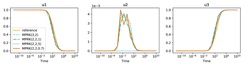
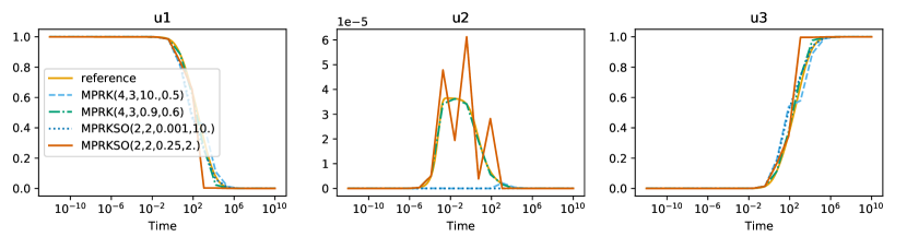
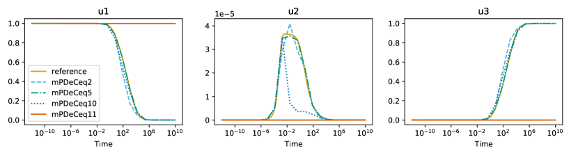
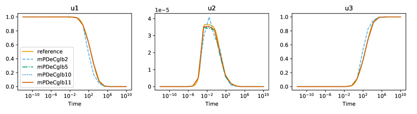
Figure 6: Robertson problem with different methods and 20 time steps.

7.2 HIRES

We consider the “High Irradiance RESponse” problem (HIRES) [17]. The original problem HIRES [32, Section II.1] can be rewritten as a nine-dimensional production–destruction system with

$$r_{1}(u)=\sigma, d_{12}(u)=k_{1}u_{1}, d_{21}(u)=k_{2}u_{2},$$ (70)

$$d_{24}(u)=k_{3}u_{2}, d_{34}(u)=k_{1}u_{3}, d_{31}(u)=k_{6}u_{3},$$

$$d_{43}(u)=k_{2}u_{4}, d_{46}(u)=k_{4}u_{4}, d_{56}(u)=k_{1}u_{5},$$

$$d_{53}(u)=k_{5}u_{5}, d_{65}(u)=k_{2}u_{6}, d_{75}(u)=\frac{k_{2}}{2}u_{7},$$

$$d_{76}(u)=\frac{k_{-}}{2}u_{7}, d_{79}(u)=\frac{k_{*}}{2}u_{7}, d_{67}(u)=k_{+}u_{6}u_{8},$$

$$d_{87}(u)=k_{+}u_{6}u_{8}, d_{78}(u)=\frac{k_{-}+k_{*}+k_{2}}{2}u_{7},$$

$p_{ij}(u)=d_{ji}\,\forall\,i,j$ and parameters

$$k_{1} =1.71, k_{2} =0.43, k_{3} =8.32, k_{4} =0.69, k_{5} =0.035,$$ (71)

$$k_{6} =8.32, k_{+} =280, k_{-} =0.69, k_{*} =0.69, \sigma =0.0007.$$

The initial condition is $u(0)=(1,0,0,0,0,0,0,0.0057,0)^{T}$, where numerically we used $10^{-35}$ instead of zero for vanishing initial constituents. The time interval is $t\in[0,321.8122]$.

MPRK(2,2,$\alpha$) with

Figure 7: Simulations of HIRES problem run with different schemes with $N=10^{3}$ time steps, plot in logarithmic scale in time.

MPRK(2,2,$\alpha$) with $\alpha=5$ mPDeC6 with Gauss–Lobatto points MPRKSO(2,2,$\alpha$,$\beta$) with $\alpha=0.3$ and $\beta=2$ For this test, the concept of oscillation is not clear as well. Nevertheless, we can observe inaccuracy of some methods also for this problem as some constituents are close to 0. We compute the reference solution with $10^{5}$ uniform time steps using mPDeC5 with equispaced sub-time steps, which is in accordance with the reference solution [32] up to the fourth significant digit for all constituents.

Testing with $N=10^{3}$ uniform time steps, we spot troubles with the inconsistent methods found in Section 6. We test the problem with many schemes presented above and we include the relative plots in the supplementary material [47]. For brevity, we plot in Figure 7.2 just a sample.

For mPDeC, we observe the loss of accuracy only for equispaced time steps for high odd orders (9, 11, 13 and so on). In Figure 7.2, we see the simulation for mPDeC6 with Gauss–Lobatto points. We observe that the high accuracy helps in obtaining a good result at the end of the simulation, when $u_{7}$ and $u_{8}$ react. The moment at which this change happens is hard to catch and only high order methods are able to obtain it within this number of time steps.

We run the MPRK(2,2,$\alpha$) with $\alpha\in\{1,5\}$. As for the linear case, we observe great loss of accuracy only for $\alpha>1$. This is demonstrated in Figure 7.2 for $\alpha=5$, where the evolution of some constituents is completely missed, e.g., $u_{2},u_{3},u_{5},u_{9}$, while for $\alpha=1$ we obtain better results.

We test MPRKSO(2,2,$\alpha$,$\beta$) with $\alpha=0.3,\,\beta=2$ and $\alpha=0,\,\beta=8$. As expected, the second one shows the spurious steady state. An oscillatory behavior can be observed, though, also in the first simulation, which is shown in Figure 7.2. This is probably due to the CFL condition; refining the time discretization, the oscillations disappear.

For MPRK(4,3,$\alpha,\beta$), we test $\alpha=0.9,\,\beta=0.6$ and $\alpha=5,\,\beta=0.5$, observing loss of accuracy only for the second one, in accordance with the linear tests. For MPRKSO(4,3), MPRK(3,2), SI-RK2 and SI-RK3, we do not observe significant loss of accuracy, as in the linear test, nor other particular behaviors.

8 Summary and discussion

We proposed an analysis for Patankar-type schemes focused on two issues that some of these schemes present: oscillations around the steady state and loss of accuracy when a constituent is not present at the initial state. The oscillations are a property strongly linked to the positivity for linear problems and it is equivalent for linear methods. On the other side, the positivity preserving Patankar-type methods are not linear, hence, they oscillate around steady states. Focusing on a generic $2\times 2$ linear test problem, we introduced an oscillation measure. Based thereon, we derived a CFL-like time step restriction avoiding oscillations for all methods under consideration, either analytically (whenever feasible) or numerically. Moreover, we investigated these methods near vanishing components, discovering order reduction phenomena in many of the modified Patankar methods, even up to first order of accuracy. Finally, we applied the methods to more challenging problems including stiff nonlinear ones. We observed that our proposed oscillation-free and accuracy analysis generalizes reasonably well to these other problems.

From our point of view, this is a first step toward further investigations on Patankar-type schemes. Extensions could be based on various Lyapunov functionals instead of our oscillation measure. Moreover, different test systems could be considered. Nevertheless, we would like to stress that our current approach seems promising and generalizes well to other demanding problems.

As mentioned in Remark 1.4, a stability analysis of all the considered methods with respect to [23] is work in progress. Furthermore, the connection between our observations and the obtained eigenvalues of the iterative process will be considered and compared in the future.

We plan also to extend our investigation to hyperbolic conservation laws. After a spatial semidiscretizations, we obtain ODEs that can be written as a production–destruction–rest system [33, 20, 11]. Here, the relation between the time step restrictions derived in this work and classical CFL conditions will be the major focus of research.

Acknowledgments

D. T. was funded by Team CARDAMOM in Inria–Bordeaux Sud–Ouest, France and by a SISSA Mathematical Fellowship, Italy. P.Ö. gratefully acknowledge support of the Gutenberg Research College, JGU Mainz and the UZH Postdoc Scholarship (Number FK-19-104). H. R. was supported by the German Research Foundation (DFG, Deutsche Forschungsgemeinschaft) under Germany’s Excellence Strategy EXC 2044-390685587, Mathematics Münster: Dynamics-Geometry-Structure. We would like to thank Stefan Kopecz and David Ketcheson for fruitful discussion at the beginning of this project. This project has started with the visit by H.R. in Zurich in 2019 which was supported by the SNF project (Number 175784) and the King Abdullah University of Science and Technology (KAUST).

Appendix A Third order modified Patankar Runge–Kutta methods

In the following part, the third order accurate MPRK(4,3,$\alpha,\beta$) from [28, 27] is repeated for completeness. Please note that the investigated version is called $MPRK43I(\alpha,\beta)$ in their papers. It is given by

$$y^{1} =u^{n}, \alpha,\beta$$ (MPRK(4,3,))

$$y^{2}_{i} =u^{n}_{i}+a_{21}\Delta tr_{i}\bigl{(}y^{1}\bigr{)}+a_{21}\Delta t\sum_{j}\left(p_{ij}\bigl{(}y^{1}\bigr{)}\frac{y^{2}_{j}}{y^{1}_{j}}-d_{ij}\bigl{(}y^{1}\bigr{)}\frac{y^{2}_{i}}{y^{1}_{i}}\right),$$

$$y^{3}_{i} =u^{n}_{i}+\Delta t\left(a_{31}r_{i}\bigl{(}y^{1}\bigr{)}+a_{32}r_{i}\bigl{(}y^{2}\bigr{)}\right)$$

$$\qquad+\Delta t\sum_{j}\Biggl{(}\left(a_{31}p_{ij}\bigl{(}y^{1}\bigr{)}+a_{32}p_{ij}\bigl{(}y^{2}\bigr{)}\right)\frac{y_{j}^{3}}{\bigl{(}y_{j}^{2}\bigr{)}^{1/p}\bigl{(}y_{j}^{1}\bigr{)}^{1-1/p}}$$

$$\qquad\qquad\qquad-\left(a_{31}d_{ij}\bigl{(}y^{1}\bigr{)}+a_{32}d_{ij}\bigl{(}y^{2}\bigr{)}\right)\frac{y_{i}^{3}}{\bigl{(}y_{i}^{2}\bigr{)}^{1/p}\bigl{(}y_{i}^{1}\bigr{)}^{1-1/p}}\Biggr{)},$$

$$\sigma_{i} =u_{i}^{n}+\Delta t\sum_{j}\Biggl{(}\left(\beta_{1}p_{ij}\bigl{(}y^{1}\bigr{)}+\beta_{2}p_{ij}\bigl{(}y^{2}\bigr{)}\right)\frac{\sigma_{j}}{\bigl{(}y_{j}^{2}\bigr{)}^{1/q}\bigl{(}y_{j}^{1}\bigr{)}^{1-1/q}}$$

$$\qquad-\left(\beta_{1}d_{ij}\bigl{(}y^{1}\bigr{)}+\beta_{2}d_{ij}\bigl{(}y^{2}\bigr{)}\right)\frac{\sigma_{i}}{\bigl{(}y_{i}^{2}\bigr{)}^{1/q}\bigl{(}y_{i}^{1}\bigr{)}^{1-1/q}}\Biggr{)}$$

$$u^{n+1}_{i} =u^{n}_{i}+\Delta t\left(b_{1}r_{i}\bigl{(}y^{1}\bigr{)}+b_{2}r_{i}\bigl{(}y^{2}\bigr{)}+b_{3}r_{i}\bigl{(}y^{3}\bigr{)}\right)$$

$$\qquad+\Delta t\sum_{j}\Biggl{(}\left(b_{1}p_{ij}\bigl{(}y^{1}\bigr{)}+b_{2}p_{ij}\bigl{(}y^{2}\bigr{)}+b_{3}p_{ij}\bigl{(}y^{3}\bigr{)}\right)\frac{u^{n+1}_{j}}{\sigma_{j}}$$

$$\qquad\qquad\qquad-\left(b_{1}d_{ij}\bigl{(}y^{1}\bigr{)}+b_{2}d_{ij}\bigl{(}y^{2}\bigr{)}+b_{3}d_{ij}\bigl{(}y^{3}\bigr{)}\right)\frac{u^{n+1}_{i}}{\sigma_{i}}\Biggr{)},$$

where $p=3a_{21}\left(a_{31}+a_{32}\right)b_{3},\;q=a_{21},\;\beta_{2}=\frac{1}{2a_{21}}$ and $\beta_{1}=1-\beta_{2}$. The Butcher tableaus in respect to the two parameters

$$\begin{array}[]{c|ccc}0&&&\\ \alpha&\alpha&&\\ \beta&\frac{3\alpha\beta(1-\alpha)-\beta^{2}}{\alpha(2-3\alpha)}&\frac{\beta(\beta-\alpha)}{\alpha(2-3\alpha)}&\\ \hline\cr&1+\frac{2-3(\alpha+\beta)}{6\alpha\beta}&\frac{3\beta-2}{6\alpha(\beta-\alpha)}&\frac{2-3\alpha}{6\beta(\beta-\alpha)}\end{array}$$ (72)

with positive coefficients for

$$\begin{rcases}2/3\leq\beta\leq 3\alpha(1-\alpha)\\ 3\alpha(1-\alpha)\leq\beta\leq 2/3\\ (3\alpha-2)/(6\alpha-3)\leq\beta\leq 2/3\end{rcases}\text{ for }\begin{cases}1/2\leq\alpha<\frac{2}{3},\\ 2/3\leq\alpha<\alpha_{0},\\ \alpha>\alpha_{0},\end{cases}$$

and $\alpha_{0}\approx 0.89255.$ When the coefficients are negative we swap the weights of production and destruction terms as for (mPDeC). Next, also the MPRKSO(4,3) from [20] is repeated. It is given by

$$y^{1} =u^{n},$$ (MPRKSO(4,3))

$$y^{2}_{i} =y^{1}_{i}+a_{10}\Delta tr_{i}\bigl{(}y^{1}\bigr{)}+\Delta t\sum_{j}b_{10}\left(p_{ij}\bigl{(}y^{1}\bigr{)}\frac{y^{2}_{j}}{y_{j}^{1}}-d_{ij}\bigl{(}y^{1}\bigr{)}\frac{y^{2}_{i}}{y_{i}^{1}}\right),$$

$$\varrho_{i} =n_{1}y_{i}^{2}+n_{2}y_{i}^{1}\left(\frac{y_{i}^{2}}{y_{i}^{1}}\right)^{2}$$

$$y^{3}_{i} =(a_{20}y^{1}_{i}+a_{21}y^{2}_{i})+\Delta t\left(b_{20}r_{i}\bigl{(}y^{1}\bigr{)}+b_{21}r_{i}\bigl{(}y^{2}\bigr{)}\right)$$

$$+\Delta t\sum_{j}\left(\left(b_{20}p_{ij}\bigl{(}y^{1}\bigr{)}+b_{21}p_{ij}\bigl{(}y^{2}\bigr{)}\right)\frac{y^{2}_{j}}{\varrho_{j}}-\left(b_{20}d_{ij}\bigl{(}y^{1}\bigr{)}+b_{21}d_{ij}\bigl{(}y^{2}\bigr{)}\right)\frac{y^{2}_{i}}{\varrho_{i}}\right),$$

$$\mu_{i} =y_{i}^{1}\left(\frac{y_{i}^{2}}{y_{i}^{1}}\right)^{s}$$

$$\tilde{a}_{i} =\eta_{1}y_{i}^{1}+\eta_{2}y_{i}^{2}+\Delta t\sum_{j}\left(\left(\eta_{3}p_{ij}\bigl{(}y^{1}\bigr{)}+\eta_{4}p_{ij}\bigl{(}y^{2}\bigr{)}\right)\frac{\tilde{a}_{j}}{\mu_{j}}-\left(\eta_{3}d_{ij}\bigl{(}y^{1}\bigr{)}+\eta_{4}d_{ij}\bigl{(}y^{2}\bigr{)}\right)\frac{\tilde{a}_{i}}{\mu_{i}}\right)$$

$$\sigma_{i} =\tilde{a}_{i}+zy_{i}^{1}\frac{y_{i}^{2}}{\varrho_{i}}$$

$$u^{n+1}_{i} =\left(a_{30}y^{1}_{i}+a_{31}y^{2}_{i}+a_{32}y^{3}_{i}\right)+\Delta t\left(b_{30}r_{i}\bigl{(}y^{1}\bigr{)}+b_{31}r_{i}\bigl{(}y^{2}\bigr{)}+b_{32}r_{i}\bigl{(}y^{3}\bigr{)}\right)$$

$$\qquad+\Delta t\sum_{j}\Biggl{(}\left(b_{30}p_{ij}\bigl{(}y^{1}\bigr{)}+b_{31}p_{ij}\bigl{(}y^{2}\bigr{)}+b_{32}p_{ij}\bigl{(}y^{3}\bigr{)}\right)\frac{u^{n+1}_{j}}{\sigma_{j}}$$

$$\qquad\qquad\qquad-\left(b_{30}d_{ij}\bigl{(}y^{1}\bigr{)}+b_{31}d_{ij}\bigl{(}y^{2}\bigr{)}+b_{32}d_{ij}\bigl{(}y^{3}\bigr{)}\right)\frac{u^{n+1}_{i}}{\sigma_{i}}\Biggr{)}.$$

Here, the optimal SSP coefficients determined in [20] will be used. They are given by

$$n_{1} =2.569046025732011E-01, n_{2} =7.430953974267989E-01,$$

$$a_{10} =1, a_{20} =9.2600312554031827E-01,$$

$$a_{21} =7.3996874459681783E-02, a_{31} =2.0662904223744017E-10,$$

$$b_{10} =4.7620819268131703E-01, a_{30} =7.0439040373427619E-01,$$

$$a_{32} =2.9560959605909481E-01, b_{20} =7.7545442722396801E-02,$$

$$b_{21} =5.9197500149679749E-01, b_{31} =6.8214380786704851E-10,$$

$$b_{30} =2.0044747790361456E-01, b_{32} =5.9121918658514827E-01,$$

$$\eta_{1} =3.777285888379173E-02, \eta_{2} =1/3,$$

$$\eta_{3} =1.868649805549811E-01, \eta_{3} =2.224876040351123,$$

$$z =6.288938077828750E-01, s =5.721964308755304.$$

Appendix B Initial correct direction of Patankar schemes

As seen in Section 4, we are looking for schemes that do not oscillate. To check this, there are two properties that must be verified. Given an arbitrary initial condition, the first step should go towards the steady state, Property 4.2, and should not overshoot the steady state, Property 4.1. In this section we investigate the direction of the first step of a method, i.e., Property 4.2. In particular, if we know that the direction of the first step is always towards the steady state, for any initial condition, we know that oscillations are possible only around the steady state. We will first present some theoretical results for very few schemes, then we summarize some numerical results we obtained varying $\varepsilon$ and $\theta$.

For symmetry we will check only Property 4.2 on the whole range of $0<\varepsilon\leq\theta<1$.

Theorem B.1 (Direction of MPE).

MPE enjoys Property 4.2 unconditionally, i.e., if the initial condition is above the steady state, then the first step will be below the initial condition, or, in other words,

$$u_{1}^{0}>(1-\theta)\Longrightarrow u_{1}^{0}>u_{1}^{1}.$$ (73)

Proof.

We write the MPE for the system (12) in the first equation, making use of the conservation property and we collect all the implicit terms.

$$u^{1}_{1} =u^{0}_{1}+\Delta t\left((1-\theta)(1-u^{0}_{1})\frac{1-u^{1}_{1}}{1-u^{0}_{1}}-\theta u^{0}_{1}\frac{u^{1}_{1}}{u^{0}_{1}}\right),$$ (74a)

$$u^{1}_{1} =u^{0}_{1}+\Delta t\left((1-\theta)(1-u^{1}_{1})-\theta u^{1}_{1}\right),$$ (74b)

$$u^{1}_{1}(1+\Delta t) =y^{1}_{1}+\Delta t(1-\theta),$$ (74c)

$$u^{1}_{1} =\frac{u^{0}_{1}+\Delta t(1-\theta)}{(1+\Delta t)}<\frac{u^{0}_{i}(1+\Delta t)}{(1+\Delta t)}=u^{0}_{1}.$$ (74d)

Here, we have simply used the hypothesis on $$u_{1}^{0}>(1-\theta)$$ and we obtain the thesis of the theorem.

∎

Theorem B.2 (Direction of MPRK(2,2,$\alpha$) with $\alpha\leq 1$).

MPRK(2,2,$\alpha$) for $\alpha\leq 1$ applied on the simplified system (12) has the correct direction of the first time step for any $\Delta t>0$.

Proof.

The first stage consists in a first MPE step with time step $\alpha\Delta t$. So we obtain that $y^{2}_{1}<y^{1}_{1}=u^{0}_{1}$.

For the second stage we can proceed analogously, exploiting the conservation property, the system (12), collecting all the implicit terms and using the hypothesis $$u^{0}_{1}>(1-\theta)$$.

$$\begin{split}u^{1}_{1}&=u^{0}_{1}+\Delta t\Biggl{(}\left(\frac{2\alpha-1}{2\alpha}(1-\theta)\bigl{(}1-y^{1}_{1}\bigr{)}+\frac{1}{2\alpha}(1-\theta)\bigl{(}1-y^{2}_{1}\bigr{)}\right)\frac{1-u^{1}_{1}}{(1-y^{2}_{1})^{1/\alpha}(1-y^{1}_{1})^{1-1/\alpha}}\\ &\qquad\qquad\qquad-\left(\frac{2\alpha-1}{2\alpha}\theta y^{1}_{1}+\frac{1}{2\alpha}\theta y^{2}_{1}\right)\frac{u^{1}_{1}}{(y^{2}_{1})^{1/\alpha}(y^{1}_{1})^{1-1/\alpha}}\Biggr{)},\end{split}$$ (75a)

$$\begin{split}u^{1}_{1}&=u^{0}_{1}+\Delta t\Biggl{(}\left(\frac{2\alpha-1}{2\alpha}(1-\theta)\left(\frac{1-y^{1}_{1}}{1-y_{1}^{2}}\right)^{1/\alpha}+\frac{1}{2\alpha}(1-\theta)\left(\frac{1-y^{2}_{1}}{1-y_{1}^{1}}\right)^{1-1/\alpha}\right)(1-u^{1}_{1})\\ &\qquad\qquad\qquad-\left(\frac{2\alpha-1}{2\alpha}\theta\left(\frac{y^{1}_{1}}{y^{2}_{1}}\right)^{1/\alpha}+\frac{1}{2\alpha}\theta\left(\frac{y^{2}_{1}}{y^{1}_{1}}\right)^{1-1/\alpha}\right)u^{1}_{1}\Biggr{)},\end{split}$$ (75b)

$$\begin{split}\Biggl{(}1+&\Delta t\left(\frac{2\alpha-1}{2\alpha}(1-\theta)\left(\frac{1-y^{1}_{1}}{1-y_{1}^{2}}\right)^{1/\alpha}+\frac{1}{2\alpha}(1-\theta)\left(\frac{1-y^{2}_{1}}{1-y_{1}^{1}}\right)^{1-1/\alpha}\right)+\\ &\Delta t\left(\frac{2\alpha-1}{2\alpha}\theta\left(\frac{y^{1}_{1}}{y^{2}_{1}}\right)^{1/\alpha}+\frac{1}{2\alpha}\theta\left(\frac{y^{2}_{1}}{y^{1}_{1}}\right)^{1-1/\alpha}\right)\Biggr{)}u^{1}_{1}=\\ u^{0}_{1}+&\Delta t\Biggl{(}\left(\frac{2\alpha-1}{2\alpha}(1-\theta)\left(\frac{1-y^{1}_{1}}{1-y_{1}^{2}}\right)^{1/\alpha}+\frac{1}{2\alpha}(1-\theta)\left(\frac{1-y^{2}_{1}}{1-y_{1}^{1}}\right)^{1-1/\alpha}\right)<\\ u^{0}_{1}&\left(1+\Delta t\Biggl{(}\left(\frac{2\alpha-1}{2\alpha}\left(\frac{1-y^{1}_{1}}{1-y_{1}^{2}}\right)^{1/\alpha}+\frac{1}{2\alpha}\left(\frac{1-y^{2}_{1}}{1-y_{1}^{1}}\right)^{1-1/\alpha}\right)\right).\end{split}$$ (75c)

So we have that

$$\begin{split}u^{1}_{1}<u_{1}^{0}\frac{N}{D}\end{split}$$ (75d)

with $$N>0 D>0 N<D N-D<0$$ and deducible from (75c). If we have our result, or, in other words, if . So, let us compute

$$\begin{split}\frac{N-D}{\Delta t}=&\frac{2\alpha-1}{2\alpha}\left(\frac{1-y^{1}_{1}}{1-y_{1}^{2}}\right)^{1/\alpha}+\frac{1}{2\alpha}\left(\frac{1-y^{2}_{1}}{1-y_{1}^{1}}\right)^{1-1/\alpha}-\\ &\frac{2\alpha-1}{2\alpha}(1-\theta)\left(\frac{1-y^{1}_{1}}{1-y_{1}^{2}}\right)^{1/\alpha}-\frac{1}{2\alpha}(1-\theta)\left(\frac{1-y^{2}_{1}}{1-y_{1}^{1}}\right)^{1-1/\alpha}-\\ &\frac{2\alpha-1}{2\alpha}\theta\left(\frac{y^{1}_{1}}{y^{2}_{1}}\right)^{1/\alpha}-\frac{1}{2\alpha}\theta\left(\frac{y^{2}_{1}}{y^{1}_{1}}\right)^{1-1/\alpha},\end{split}$$ (75e)

$$\begin{split}\frac{N-D}{\Delta t}=&\frac{2\alpha-1}{2\alpha}\theta\left(\frac{1-y^{1}_{1}}{1-y_{1}^{2}}\right)^{1/\alpha}+\frac{1}{2\alpha}\theta\left(\frac{1-y^{2}_{1}}{1-y_{1}^{1}}\right)^{1-1/\alpha}-\\ &\frac{2\alpha-1}{2\alpha}\theta\left(\frac{y^{1}_{1}}{y^{2}_{1}}\right)^{1/\alpha}-\frac{1}{2\alpha}\theta\left(\frac{y^{2}_{1}}{y^{1}_{1}}\right)^{1-1/\alpha}=\\ &\frac{2\alpha-1}{2\alpha}\theta\left(\left(\frac{1-y^{1}_{1}}{1-y_{1}^{2}}\right)^{1/\alpha}-\left(\frac{y^{1}_{1}}{y^{2}_{1}}\right)^{1/\alpha}\right)+\frac{1}{2\alpha}\theta\left(\left(\frac{1-y^{2}_{1}}{1-y_{1}^{1}}\right)^{1-1/\alpha}-\left(\frac{y^{2}_{1}}{y^{1}_{1}}\right)^{1-1/\alpha}\right).\end{split}$$ (75f)

Now, we know that $$y_{1}^{1}>y^{2}_{1} 0<\alpha\leq 1 1/\alpha>0 1-1/\alpha\leq 0 \frac{N-D}{\Delta t}<0$$, hence y11y12>1>1-y111-y12, so, considering , we have that and , we have ((1-y111-y12)^1/α -(y11y21)^1/α )<0 and ((1-y211-y11)^1-1/α- ( y21y11)^1-1/α )<0. Hence, and the proof is complete.

∎

For the case with $\alpha>1$ it is not so easy to derive an estimation as the two terms have opposite signs.

Theorem B.3 (Direction of MPRKSO(2,2,$\alpha$,$\beta$) with $\gamma\geq 1$).

MPRKSO(2,2,$\alpha$,$\beta$) applied on the simplified system (12) for positive RK coefficients and for γ=1-αβ+ αβ2β(1-αβ)≥1 has the correct direction of the first time step.

Proof.

The proof follows the same step of proof of Theorem B.2. The condition on the exponent of the weights here is precisely $\gamma\geq 1$. ∎

Remark B.4 (Accuracy area).

We want to remark that the area in the $(\alpha,\beta)$ plane where $\gamma\geq 1$ and the RK coefficients are positive is defined by α≤β-12β2-β with β≥1, and this area coincide with the second order area for vanishing IC of MPRKSO(2,2,$\alpha$,$\beta$) found in Figure 4(b).

B.1 Initial direction of other schemes

For all other schemes it is not so easy to prove directly that the direction of the first step is the correct one. Nevertheless, we checked symbolically (when feasible) and numerically (otherwise) this property. The numerical computations are included in CheckingDirection.ipynb in the repository [46], while the only theoretical result is in MPRK_3_2.nb. We summarize in the following the results we obtained.

Figure 8: Simulation of (12) with $\theta=4\cdot 10^{-4}$ and $u_{2}^{0}=\varepsilon=2\cdot 10^{-6}$ with mPDeC8 with equispaced points for $\Delta t=64$

• MPRK(3,2) has the correct direction and we proved it in the Mathematica notebook MPRK_3_2.nb;

• MPRK(2,2,$\alpha$) have the correct direction for all $1/2\leq\alpha\leq 4$;

• MPRKSO(2,2,$\alpha$,$\beta$) have the correct direction in an area slightly larger than the positive RK weights area displayed in Figure 5(d), which coincide with the strictly positive $\Delta t$ bound area there;

• MPRK(4,3,$\alpha,\beta$) have the correct direction except in a small area around $\alpha=2/3$ where the RK coefficients are negative;

• MPRKSO(4,3) has the correct direction;

• mPDeC with Gauss–Lobatto points have the correct direction (tested up to order 16);

• mPDeC with equispaced points have the correct direction up to order 7, for order 8, 9 and 15 we found wrong directions for large $\Delta t(\geq 30)$ and very small initial conditions and $\theta$, all other mPDeC with orders up to 16 have the correct direction;

• SI-RK2 and SI-RK3 have the correct direction.

In Figure 8, we show an example for mPDeC8 where the correct direction is not followed. We see that even if we go away from the steady state, the scheme does not oscillate.

References

• [1] Rémi Abgrall “High order schemes for hyperbolic problems using globally continuous approximation and avoiding mass matrices” In Journal of Scientific Computing 73.2 Springer, 2017, pp. 461–494
• [2] Andrés I. Ávila, Stefan Kopecz and Andreas Meister “A comprehensive theory on generalized BBKS schemes” In Applied Numerical Mathematics 157 Elsevier, 2020, pp. 19–37
• [3] Owe Axelsson “Iterative Solution Methods” Cambridge: Cambridge University Press, 1996 DOI: 10.1017/CBO9780511624100
• [4] Alfredo Bellen and Lucio Torelli “Unconditional Contractivity in the Maximum Norm of Diagonally Split Runge–Kutta Methods” In SIAM Journal on Numerical Analysis 34.2 SIAM, 1997, pp. 528–543 DOI: 10.1137/S0036142994267576
• [5] Jeff Bezanson, Alan Edelman, Stefan Karpinski and Viral B Shah “Julia: A Fresh Approach to Numerical Computing” In SIAM Review 59.1 SIAM, 2017, pp. 65–98 DOI: 10.1137/141000671
• [6] Catherine Bolley and Michel Crouzeix “Conservation de la positivité lors de la discrétisation des problèmes d’évolution paraboliques” In RAIRO. Analyse numérique 12.3 EDP Sciences, 1978, pp. 237–245
• [7] N. Broekhuizen, G. J. Rickard, J. Bruggeman and A. Meister “An improved and generalized second order, unconditionally positive, mass conserving integration scheme for biochemical systems” In Applied numerical mathematics 58.3 Elsevier, 2008, pp. 319–340
• [8] Jorn Bruggeman, Hans Burchard, Bob W Kooi and Ben Sommeijer “A second-order, unconditionally positive, mass-conserving integration scheme for biochemical systems” In Applied numerical mathematics 57.1 Elsevier, 2007, pp. 36–58
• [9] Hans Burchard, Eric Deleersnijder and Andreas Meister “A high-order conservative Patankar-type discretisation for stiff systems of production–destruction equations” In Applied Numerical Mathematics 47.1 Elsevier, 2003, pp. 1–30 DOI: 10.1016/S0168-9274(03)00101-6
• [10] Alina Chertock, Shumo Cui, Alexander Kurganov and Tong Wu “Steady state and sign preserving semi-implicit Runge–Kutta methods for ODEs with stiff damping term” In SIAM Journal on Numerical Analysis 53.4 SIAM, 2015, pp. 2008–2029 DOI: 10.1137/151005798
• [11] Mirco Ciallella, Lorenzo Micalizzi, Philipp Öffner and Davide Torlo “An Arbitrary High Order and Positivity Preserving Method for the Shallow Water Equations”, arXiv preprint: https://arxiv.org/abs/2108.07347, 2021 arXiv:2110.13509 [math.NA]
• [12] Imre Fekete, David I. Ketcheson and Lajos Lóczi “Positivity for convective semi-discretizations” In Journal of Scientific Computing 74.1 Springer, 2018, pp. 244–266 DOI: 10.1007/s10915-017-0432-9
• [13] L. Formaggia and A. Scotti “Positivity and Conservation Properties of Some Integration Schemes for Mass Action Kinetics” In SIAM Journal on Numerical Analysis 49.3, 2011, pp. 1267–1288 DOI: 10.1137/100789592
• [14] Peter Frolkovic “Semi-implicit methods based on inflow implicit and outflow explicit time discretization of advection” In Proceedings of ALGORITMY, 2016, pp. 165–174
• [15] Sigal Gottlieb, David I. Ketcheson and Chi-Wang Shu “Strong stability preserving Runge–Kutta and multistep time discretizations” Singapore: World Scientific, 2011
• [16] Ernst Hairer, Syvert Paul Norsett and Gerhard Wanner “Solving Ordinary, Differential Equations I, Nonstiff problems/E. Hairer, SP Norsett, G. Wanner, with 135 Figures, Vol.: 1” 2Ed. Springer-Verlag, 2000, 2000
• [17] Ernst Hairer and Gerhard Wanner “Stiff differential equations solved by Radau methods” In Journal of Computational and Applied Mathematics 111.1-2 Elsevier, 1999, pp. 93–111 DOI: 10.1016/S0377-0427(99)00134-X
• [18] Zoltán Horváth “Positivity of Runge–Kutta and diagonally split Runge–Kutta methods” In Applied Numerical Mathematics 28.2-4 Elsevier, 1998, pp. 309–326 DOI: 10.1016/S0168-9274(98)00050-6
• [19] Juntao Huang and Chi-Wang Shu “Positivity-Preserving Time Discretizations for Production–Destruction Equations with Applications to Non-equilibrium Flows” In Journal of Scientific Computing 78.3 Springer, 2019, pp. 1811–1839 DOI: 10.1007/s10915-018-0852-1
• [20] Juntao Huang, Weifeng Zhao and Chi-Wang Shu “A Third-Order Unconditionally Positivity-Preserving Scheme for Production–Destruction Equations with Applications to Non-equilibrium Flows” In Journal of Scientific Computing 79.2 Springer, 2019, pp. 1015–1056 DOI: 10.1007/s10915-018-0881-9
• [21] Karel J. in’ t Hout “A note on unconditional maximum norm contractivity of diagonally split Runge–Kutta methods” In SIAM Journal on Numerical Analysis 33.3 SIAM, 1996, pp. 1125–1134 DOI: 10.1137/0733055
• [22] Thomas Izgin, Stefan Kopecz and Andreas Meister “On Lyapunov Stability of Positive and Conservative Time Integrators and Application to Second Order Modified Patankar–Runge–Kutta Schemes” In arXiv preprint arXiv:2202.01099, 2022
• [23] Thomas Izgin, Stefan Kopecz and Andreas Meister “On the Stability of Unconditionally Positive and Linear Invariants Preserving Time Integration Schemes” In arXiv preprint arXiv:2202.11649, 2022
• [24] Thomas Izgin, Stefan Kopecz and Andreas Meister “Recent Developments in the Field of Modified Patankar-Runge-Kutta-methods” In PAMM 21.1 Wiley Online Library, 2021, pp. e202100027
• [25] Stefan Kopecz and Andreas Meister “A comparison of numerical methods for conservative and positive advection–diffusion–production–destruction systems” In PAMM 19.1 Wiley Online Library, 2019 DOI: 10.1002/pamm.201900209
• [26] Stefan Kopecz and Andreas Meister “On order conditions for modified Patankar–Runge–Kutta schemes” In Applied Numerical Mathematics 123 Elsevier, 2018, pp. 159–179 DOI: 10.1016/j.apnum.2017.09.004
• [27] Stefan Kopecz and Andreas Meister “On the existence of three-stage third-order modified Patankar–Runge–Kutta schemes” In Numerical Algorithms Springer, 2019, pp. 1–12 DOI: 10.1007/s11075-019-00680-3
• [28] Stefan Kopecz and Andreas Meister “Unconditionally positive and conservative third order modified Patankar–Runge–Kutta discretizations of production–destruction systems” In BIT Numerical Mathematics 58.3 Springer, 2018, pp. 691–728 DOI: 10.1007/s10543-018-0705-1
• [29] Dmitri Kuzmin “Entropy stabilization and property-preserving limiters for $\mathbb{P}^{1}$ discontinuous Galerkin discretizations of scalar hyperbolic problems” In Journal of Numerical Mathematics De Gruyter, 2020
• [30] Colin B. Macdonald, Sigal Gottlieb and Steven J. Ruuth “A numerical study of diagonally split Runge–Kutta methods for PDEs with discontinuities” In Journal of Scientific Computing 36.1 Springer, 2008, pp. 89–112 DOI: 10.1007/s10915-007-9180-6
• [31] Angela Martiradonna, Gianpiero Colonna and Fasma Diele “GeCo: Geometric Conservative nonstandard schemes for biochemical systems” In Applied Numerical Mathematics 155, 2020, pp. 38–57 DOI: 10.1016/j.apnum.2019.12.004
• [32] Francesca Mazzia and Cecilia Magherini “Test Set for Initial Value Problem Solvers”, 2008
• [33] Andreas Meister and Sigrun Ortleb “A positivity preserving and well-balanced DG scheme using finite volume subcells in almost dry regions” In Applied Mathematics and Computation 272 Elsevier, 2016, pp. 259–273
• [34] Karol Mikula and Mario Ohlberger “Inflow-implicit/outflow-explicit scheme for solving advection equations” In Finite Volumes for Complex Applications VI Problems & Perspectives 4, Springer Proceedings in Mathematics Berlin, Heidelberg: Springer, 2011, pp. 683–691 DOI: 10.1007/978-3-642-20671-9_72
• [35] Karol Mikula, Mario Ohlberger and Jozef Urbán “Inflow-implicit/outflow-explicit finite volume methods for solving advection equations” In Applied Numerical Mathematics 85 Elsevier, 2014, pp. 16–37 DOI: 10.1016/j.apnum.2014.06.002
• [36] Stephan Nüßlein, Hendrik Ranocha and David I Ketcheson “Positivity-Preserving Adaptive Runge-Kutta Methods” In Communications in Applied Mathematics and Computational Science 16.2, 2021, pp. 155–179 DOI: 10.2140/camcos.2021.16.155
• [37] Philipp Öffner and Davide Torlo “Arbitrary high-order, conservative and positivity preserving Patankar-type deferred correction schemes” In Applied Numerical Mathematics 153 Elsevier, 2020, pp. 15–34
• [38] Suhas V Patankar “Numerical Heat Transfer and Fluid Flow” Washington: Hemisphere Publishing Corporation, 1980
• [39] Orson Pratt “New and Easy Method of Solution of the Cubic Biquadratic Equations: Embracing Several New Formulas, Greatly Simplifying this Department of Mathematical Science” Liverpool: Longmans, Green, Reader,Dyer, 1866
• [40] Christopher Rackauckas and Qing Nie “DifferentialEquations.jl – A Performant and Feature-Rich Ecosystem for Solving Differential Equations in Julia” In Journal of Open Research Software 5.1 Ubiquity Press, 2017, pp. 15 DOI: 10.5334/jors.151
• [41] Hendrik Ranocha “On strong stability of explicit Runge–Kutta methods for nonlinear semibounded operators” In IMA Journal of Numerical Analysis 41.1 Oxford University Press, 2021, pp. 654–682
• [42] Hendrik Ranocha and David I. Ketcheson “Energy Stability of Explicit Runge–Kutta Methods for Nonautonomous or Nonlinear Problems” In SIAM Journal on Numerical Analysis 58.6 SIAM, 2020, pp. 3382–3405
• [43] Hendrik Ranocha and Philipp Öffner $L_{2}$ Stability of Explicit Runge–Kutta Schemes” In Journal of Scientific Computing 75.2, 2018, pp. 1040–1056 DOI: 10.1007/s10915-017-0595-4
• [44] Zheng Sun and Chi-Wang Shu “Stability of the fourth order Runge–Kutta method for time-dependent partial differential equations” In Annals of Mathematical Sciences and Applications 2.2, 2017, pp. 255–284 DOI: 10.4310/AMSA.2017.v2.n2.a3
• [45] Zheng Sun and Chi-Wang Shu “Strong Stability of Explicit Runge–Kutta Time Discretizations” In SIAM Journal on Numerical Analysis 57.3 SIAM, 2019, pp. 1158–1182 DOI: 10.1137/18M122892X
• [46] Davide Torlo, Philipp Öffner and Hendrik Ranocha “Issues with Positivity Preserving Patankar-Type Schemes”, Git repository: https://git.math.uzh.ch/abgrall_group/patankar-stability, 2021
• [47] Davide Torlo, Philipp Öffner and Hendrik Ranocha “Issues with Positivity-Preserving Patankar-type Schemes”, arXiv preprint: https://arxiv.org/abs/2108.07347, 2021 arXiv:2108.07347 [math.NA]