Fermions on a torus knot

Abstract

In this work, we investigate the effects of a nontrivial topology (and geometry) of a system considering interacting and noninteracting particle modes, which are restricted to follow a closed path over the torus surface. In order to present a prominent thermodynamical investigation of this system configuration, we carry out a detailed analysis using statistical mechanics within the grand canonical ensemble approach to deal with noninteracting fermions. In an analytical manner, we study the following thermodynamic functions in such context: the Helmholtz free energy, the mean energy, the magnetization and the susceptibility. Further, we take into account the behavior of Fermi energy of the thermodynamic system. Finally, we briefly outline how to proceed in case of interacting fermions.

I Introduction

The knowledge of thermodynamic properties of many body systems plays an essential role in condensed matter physics, especially in case of developing new materials gaskell2012introduction ; muhlschlegel1972thermodynamic ; dehoff2006thermodynamics ; jones1974thermodynamics ; davidovits1991geopolymers ; safran2018statistical ; bates1990block . Electrons in metals, under widely varying circumstances, behave as free particles and can be treated as an electron gas under certain approximations araujo2017structural ; silva2018polarized ; casida1998molecular ; lee1988development ; segall2002first ; perdew1981self ; perdew1986density ; perdew1992accurate ; perdew1996generalized . In this regard, surface effects such as shape dependence dai2003quantum ; dai2004geometry ; potempa1998dependence and nontrivial topology angelani2005topology ; bendsoe2013topology ; oliveira2020relativistic ; narang2021topology can lead to some novel and unexpected features. A generic computational problem is to derive the partition function that requires a sum over all accessible quantum states landau2013course ; reichl1999modern ; huang2009introduction . For higher temperatures, the particle effective wavelength turns out to be too short in comparison with the characteristic dimension of the system and, therefore, the boundary effects can be overlooked. Previously, such idea was exploited by Rayleigh and Jeans in the radiation theory of electromagnetism zettili2003quantum ; purcell1965electricity ; tipler2003modern ; moreover, this was corroborated in a purely mathematical framework by Weyl weyl1968gesammelte .

Quantum mechanics of particle on a torus knot was analyzed in Ref. sreedhar2015classical . Further topological aspects such as Berry phase and Hannay angle features to this model were investigated in ghosh2018particle ; das2016particle ; biswas2020quantum ; in particular, curvature and torsion effects of the knotted path were also taken into account. The generic problem of a quantum particle restricted to a curved path or to a general surface, was considered earlier in da1981quantum ; wang2018geometric ; ortix2015quantum ; da2017quantum ; ferrari2008schrodinger .

Knot theory is a well known branch of pure mathematics tu2011manifolds ; tu2017differential . The quantum mechanics on particles on torus knot can be motivated by the carbon nanorings (made from carbon nanotubes liu2001structural ) that are intimately connected to the edges of nanotubes, nanochains, graphene, and nanocones kharissova2019inorganic ; chen2005mechanical . Such nanorings (or nanotori) have a variety of notable features, being mostly investigated in generic calculations madani2012energies and specializing in multiresonant properties lewicka2013nanorings , magneto-optical activity feng2014magnetoplasmonic , paramagnetism liu2002colossal , and ferromagnetism vojkovic2016magnetization ; rodriguez2004magnetism . Moreover, these present nanostructures may also be employed in optical communications du2014silicon , isolators, traps for ions and atoms chan2012carbon , and lubricants pena2019novel .

In this sense, the present work is aimed at studying the topological effects of a novel thermodynamic system comprising a gas of fermions, that follows a closed path with nontrivial knot structure on the surface of a torus. For convenience, one might visualize the particles moving within a carbon nanotube wound around the torus in the form of a knot. Furthermore, we calculate the Helmholtz free energy, mean energy, magnetization and susceptibility of the system. In our investigation, we exploit the formalism of araujo2021thermal ; reis2020does to derive the thermodynamic quantities – using results from das2016particle , for both interacting and noninteracting fermion particles.

The paper is organized as follows: in Section II, the basic formalism and notations are set up by considering a system of noninteracting particles and analytic expressions of all the thermodynamic quantities are computed starting from the partition function. Noninteracting fermions were introduced in Section III and, together with other observables, the Fermi energy is also studied. In Section IV, we outline the way to incorporate interactions in the fermionic model. The paper is concluded with a summary of the results obtained in Section V.

II Statistical mechanics of $N$ particles in a torus knot subjected to a magnetic field

Let us consider an ensemble composed of $N$ particles moving on a single torus in a prescribed path. For the situation that we are considering, the canonical ensemble theory is sufficient to describe this case. The partition function for the system of $N$ particle is given by

$$\mathcal{Z}=\sum_{\left\{\Omega\right\}}\exp\left(-\beta E_{\Omega}\right),$$ (1)

where $\Omega$ is related to all accessible quantum states. Since we are dealing with noninteracting particles, the partition function $\left(\ref{eq:Partition-function}\right)$ can be factorized, giving the following result below

$$\mathcal{Z}=\mathcal{Z}_{1}^{N}=\left\{\sum_{\left\{\Omega\right\}}\exp\left(-\beta E_{\Omega}\right)\right\}^{N},$$ (2)

where we have defined the single partition function as

$$\mathcal{Z}_{1}=\sum_{\Omega}\exp\left(-\beta E_{\Omega}\right).$$ (3)

It is interesting to point out that, even though the underling geometry is not a simply connected one, there is no problem in regarding the factorization above, since there is no interaction potential generated by the geometry itself. This affirmation can naturally be checked by looking at the energy spectrum given by Eq. 8. The connection with macroscopic thermodynamic observables can be given by Helmholtz free energy

$$f=-\frac{1}{\beta}\lim_{N\rightarrow\infty}\frac{1}{N}\ln\mathcal{Z},$$ (4)

where $f$ stands for the Helmholtz free energy per particle. With this quantity, we can derive the following thermodynamic state functions

$$s=-\frac{\partial f}{\partial T},\phantom{ss}c=T\frac{\partial s}{\partial T},\phantom{ss}u=-\frac{\partial}{\partial\beta}\ln\mathcal{Z},$$ (5)

where $s,c,u$ represent entropy, heat capacity and energy per particle, respectively. We can also calculate magnetization $\mathfrak{m}$ and susceptibility $\chi$ with respect to the external magnetic $B$, as given by

$$\mathfrak{m}=-\frac{\partial f}{\partial B},\phantom{ss}\chi=\frac{\partial\mathfrak{m}}{\partial B}.$$ (6)

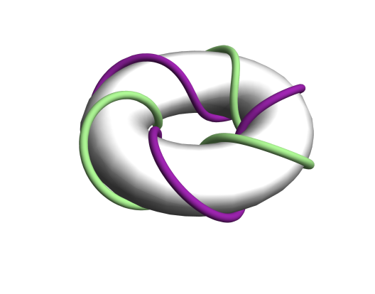
Figure 1: A representation of a torus knot (2,3). The wire represents the path followed by the particles on its surface

The sum in Eq. $\left(\ref{eq:Single-Partition-function}\right)$ can be brought to a closed form by using the well-know Euler-MacLaurin formula oliveira2019thermodynamic ; oliveira2020thermodynamic

$$\sum_{n=0}^{\infty}F\left(n\right)=\int_{0}^{\infty}F\left(n\right)dn+\frac{1}{2}F\left(0\right)-\frac{1}{2!}B_{2}F^{\prime}\left(0\right)-\frac{1}{4!}B_{4}F^{\prime\prime\prime}\left(0\right)+\ldots,$$ (7)

which allows us to perform the calculation exactly. The energy spectrum of a particle moving on a torus with dimensions $a,d$ and submitted to a uniform magnetic field that points along the $\boldsymbol{\hat{z}}$ direction is given by das2016particle

$$E_{n}=\frac{1}{2m}\left[\frac{n^{2}\hbar^{2}}{p^{2}d^{2}}\left(1-\frac{a^{2}q^{2}}{p^{2}d^{2}}\right)+\frac{eB}{p}n\hbar\left(1+\frac{a^{2}}{2d^{2}}-\frac{a^{2}q^{2}}{p^{2}d^{2}}\right)+\frac{e^{2}B^{2}d^{2}}{4}\left(1+\frac{a^{2}}{d^{2}}-\frac{a^{2}q^{2}}{p^{2}d^{2}}\right)\right],$$ (8)

where $d$ is the outer radius and $a$ the internal radius of the torus respectively with ($d>a$) (see Fig. 1). The closed path is characterized by a $(p,q)$-knot with $p$ and $q$ denoting the toroidal and poloidal turns, respectively, so that it turns around $d$ and $a$ respectively. For a nontrivial torus knot, $(p,q)$ are coprime numbers. The well known and simplest knot, a $(2,3)$ or trefoil knot, is depicted in Fig. 1.

Now inserting the energy spectrum on the single partition function (1) and computing the sum, we are led to the following single particle partition function:

$$\mathcal{Z}_{1} = \sqrt{\frac{\pi mp^{2}d^{2}}{2\beta\left(1-\mathcal{A}\right)}}\exp\left[\beta\frac{d\alpha^{2}\mathcal{A}}{32m\left(1-\mathcal{A}\right)}\xi\right]\times$$ (9)

$$\times\left\{1+\mathrm{erf}\left[-\frac{\xi}{4}\sqrt{\frac{2\beta}{m\left(1-\mathcal{A}\right)}}\left(1-\mathcal{A}+\frac{\alpha^{2}}{2}\mathcal{A}\right)\right]\right\},$$

where $\mathrm{erf}$ is the error function given by

$$\mathrm{erf}\left[z\right]=\frac{2}{\sqrt{\pi}}\int_{0}^{z}e^{-t^{2}}dt,$$ (10)

and we also have defined the following quantities

$$\xi=eB,\phantom{ss}\mathcal{A}=\frac{a^{2}}{d^{2}},\phantom{ss}\alpha=\frac{q}{p},$$ (11)

where $\mathcal{A}$ is a property of the torus whereas $\alpha$ characterizes the knot of the particular path. The quantity $\alpha$ is called the “winding number” of the $(p,q)$-torus knot, and it is also a simple way of measuring the complexity of the knot. Notice that two different torus knots can have the same $\alpha$. Nevertheless, $\alpha$ will be different if at least one of $p$ or $q$ differ. In this sense, $\alpha$ is regarded as a “unique” identity of a $(p,q)$-torus knot. It is worth mentioning that similar forms of partition function have appeared in very recent works in the literature considering different contexts araujo2021thermodynamic ; araujo2021lorentz ; petrov2021higher ; petrov2021bouncing ; aa2021thermodynamics22 .

Now substituting $\left(\ref{eq:Exact_Z}\right)$ in $\left(\ref{eq:Helmm-f}\right)$, we find

$$f = -\frac{d\alpha^{2}\mathcal{A}}{32m\left(1-\mathcal{A}\right)}\xi-\frac{1}{\beta}\ln\sqrt{\frac{\pi mp^{2}d^{2}}{2\beta\left(1-\mathcal{A}\right)}}$$ (12)

$$-\frac{1}{\beta}\ln\left\{1+\mathrm{erf}\left[-\frac{\xi}{4}\sqrt{\frac{2\beta}{m\left(1-\mathcal{A}\right)}}\left(1-\mathcal{A}+\frac{\alpha^{2}}{2}\mathcal{A}\right)\right]\right\}.$$

From this expression, using previous relations (5), we can get the relevant thermodynamic variables. For instance, the internal energy is given by

$$u = -\frac{1}{\beta^{2}}\left(\frac{1}{2}+\ln\sqrt{\frac{\pi mp^{2}d^{2}}{2\beta\left(1-\mathcal{A}\right)}}\right)$$ (13)

$$-\frac{1}{\beta^{2}}\ln\left\{1+\mathrm{erf}\left[-\frac{\xi}{4}\sqrt{\frac{2\beta}{m\left(1-\mathcal{A}\right)}}\left(1-\mathcal{A}+\frac{\alpha^{2}}{2}\mathcal{A}\right)\right]\right\}$$

$$-\frac{\xi}{\beta^{\frac{3}{2}}}\sqrt{\frac{1}{8m\pi\left(1-\mathcal{A}\right)}}\frac{\left(1-\mathcal{A}+\frac{\alpha^{2}}{2}\mathcal{A}\right)\exp\left[-\frac{\xi^{2}}{8}\frac{\beta}{m\left(1-\mathcal{A}\right)}\left(1-\mathcal{A}+\frac{\alpha^{2}}{2}\mathcal{A}\right)^{2}\right]}{1-\mathrm{erf}\left[\frac{\xi}{4}\sqrt{\frac{2\beta}{m\left(1-\mathcal{A}\right)}}\left(1-\mathcal{A}+\frac{\alpha^{2}}{2}\mathcal{A}\right)\right]}.$$

Another important quantity is the magnetization, which reads

$$\mathfrak{m}=\frac{d\alpha^{2}\mathcal{A}}{32m\left(1-\mathcal{A}\right)}-\sqrt{\frac{1}{2\pi\beta m\left(1-\mathcal{A}\right)}}\frac{\left(1-\mathcal{A}+\frac{\alpha^{2}}{2}\mathcal{A}\right)\exp\left[-\frac{\xi^{2}}{8}\frac{\beta}{m\left(1-\mathcal{A}\right)}\left(1-\mathcal{A}+\frac{\alpha^{2}}{2}\mathcal{A}\right)^{2}\right]}{1-\mathrm{erf}\left[\frac{\xi}{4}\sqrt{\frac{2\beta}{m\left(1-\mathcal{A}\right)}}\left(1-\mathcal{A}+\frac{\alpha^{2}}{2}\mathcal{A}\right)\right]}.$$ (14)

The susceptibility can also be calculated and is given by

$$\chi=-\frac{4}{\pi\beta}\frac{\mathcal{B}^{2}\exp\left(-2\mathcal{B}^{2}\xi^{2}\right)}{1-\mathrm{erf}\left(\mathcal{B}\xi\right)}\left\{\frac{1}{1-\mathrm{erf}\left(\mathcal{B}\xi\right)}-\sqrt{\pi}\mathcal{B}\xi\exp\left(\mathcal{B}^{2}\xi^{2}\right)\right\},$$ (15)

where we have used the shorthand notation

$$\mathcal{B}=\frac{1}{4}\sqrt{\frac{2\beta}{m\left(1-\mathcal{A}\right)}}\left(1-\mathcal{A}+\frac{\alpha^{2}}{2}\mathcal{A}\right).$$ (16)

Since expressions of energy, magnetization and susceptibility are quite lengthy, instead of providing their explicit forms, we show their behavior pictorially. Similarly, in this way, for entropy and heat capacity in the low energy regime, we shall follow the same procedure. Let us explore some interesting features from the magnetization and the susceptibility for a particular configuration of magnetic field and temperature. Initially, we consider the configuration in which $\xi=0$. With this, we obtain the following results:

$$\mathfrak{m}_{\xi=0} =\frac{d\alpha^{2}\mathcal{A}}{32m\left(1-\mathcal{A}\right)}-\frac{1-\mathcal{A}+\frac{\alpha^{2}}{2}\mathcal{A}}{\sqrt{2\pi\beta m\left(1-\mathcal{A}\right)}},$$ (17)

$$\chi_{\xi=0} =-\frac{4\mathcal{B}^{2}}{\pi\beta}.$$ (18)

Now, for both $\xi=0$ and $T=0$, we get

$$\mathfrak{m}_{\xi=0,T=0} =\frac{d\alpha^{2}\mathcal{A}}{32m\left(1-\mathcal{A}\right)},$$ (19)

$$\chi_{\xi=0,T=0} =-\frac{1}{2\pi}\frac{1}{m\left(1-\mathcal{A}\right)}\left(1-\mathcal{A}+\frac{\alpha^{2}}{2}\mathcal{A}\right)^{2}.$$ (20)

It is interesting to note that in the above restricted cases, the topology of the path appears only through $\alpha$ whereas both $a,d$ appear to represent geometry of the path. Furthermore, the residual magnetization and susceptibility are mainly characterized by its geometrical and topological aspects. For instance, if the topological parameter $\alpha$ increases, then both $\mathfrak{m}_{\xi=0,T=0}$ and $\chi_{\xi=0,T=0}$ increase as well their magnitude. Therefore, the residual magnetic properties will depend on the complexities of the path that the electrons follow.

In Figs. 2, 3 and 4, we have used the values $p=2$ and $q=3$, so that the first coprimes yielding the simplest and widely studied $(2,3)$-knot or the trefoil knot. The plots below exhibit the behavior of the thermodynamic functions with respect to the temperature. Moreover, we also compare the behavior of those functions for different values of the parameter $\xi$, which controls the intensity of the external magnetic field. Since our system consists of electrons, we need to take its mass into account in our numerical calculations.

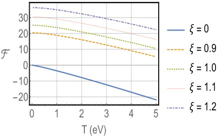
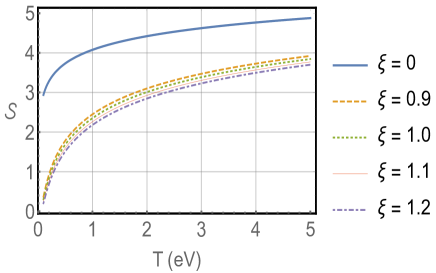
Figure 2: Helmholtz free energy $({\cal{F}})$ and entropy $({\cal{S}})$ versus temperature ($T$)

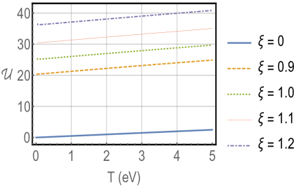
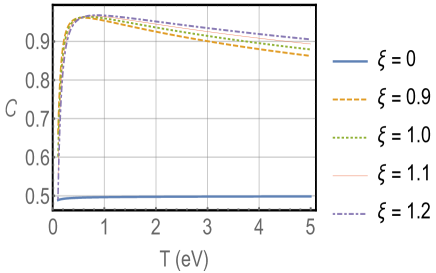
Figure 3: Internal energy $({\cal{U}})$ and Heat capacity $({\cal{C}})$ versus temperature ($T$)

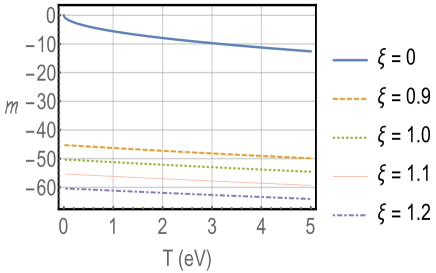
Figure 4: Magnetization $({\cal{M}})$ and Susceptibility $({\cal{\chi}})$ versus temperature ($T$)

In order to acquire a better understanding of the behavior of the thermodynamic functions for different combinations of toroidal and poloidal windings $p$ and $q$, we display below the contour plot of such functions with respect to certain ranges of winding numbers, as displayed in Figs. 5, 6, 7, 8, 9, and 10. Unlike the special cases of zero magnetic field and/or zero temperature, in general situations, the thermodynamic observables depend on both $p,q$ individually (i.e. not only on $\alpha$).

The plots mainly compare how those functions behave for a given temperature and magnetic field. Initially, in Fig. 5, we see the Helmholtz free energy for different fixed values of temperature and magnetic field – the variable combinations of winding numbers $(p,q)$, including co-prime $p,q$, satisfy the knot condition. We see in all configurations that the larger the values of $(p,q)$, the larger the Helmholtz energy becomes. In Fig. 6, we also investigate how entropy is modified for different configurations of temperature and magnetic field. It is shown the behavior of the entropy as a function of the winding numbers $(p,q)$. In short, we verify that in all configurations when we increase values of $(p,q)$, entropy increases. Next, in Fig. 7, we provide the contour plot for the mean energy regarding different configurations of temperature and magnetic field as well. We see that in all configurations when $q$ is increased for fixed $p$, the mean energy decreases; on the other hand, when the values of $p$ increase maintaining $q$ fixed, the opposite behavior occurs. Fig. 8 displays contour plots to the heat capacity for different values of temperature and magnetic field. In these ones, we can naturally see the behavior of the heat capacity as a function of the winding numbers $(p,q)$. We see that in all configurations when we increase the values of $q$ keeping $p$ fixed, the heat capacity decreases its values; on the other hand, if we have the values of $p$ increased maintaining $q$ fixed, the opposite behavior also occurs. In Fig. 9, we also show the plots exhibiting how the magnetization is affected by different configurations of temperature and magnetic field. Here, we realize the behavior of the magnetization as a function of the winding numbers $(p,q)$. Thereby, we see that in all configurations when we increase the values of $(p,q)$, the larger the magnetization becomes. Finally, in Fig. 10, the plots exhibit how the the susceptibility is changed for different temperature and magnetic field. In this sense, we see the behavior of the susceptibility as a function of the winding numbers $(p,q)$. Furthermore, we verify that in all configurations when we increase the values of $(p,q)$, susceptibility becomes larger.

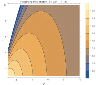
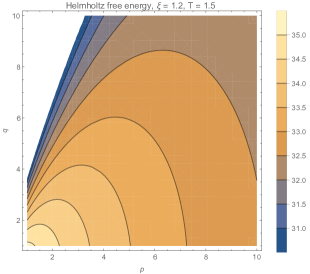
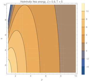
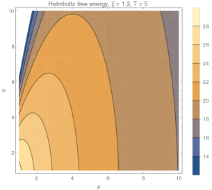
Figure 5: These plots exhibit the Helmholtz free energy for different configurations of temperature and magnetic field. It also displays the behavior of Helmholtz energy as a function of the wind numbers $(p,q)$. Note that Free energy increases when magnetic field increases and also when both $p$ and $q$ increases.

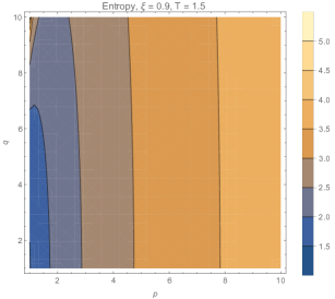
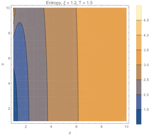
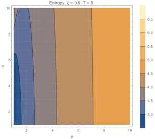
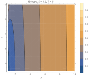
Figure 6: These plots exhibit the entropy for different configurations of temperature and magnetic field. We also see its behavior as a function of the wind numbers $(p,q)$. The behavior of the entropy is similar to the free energy, i.e. it increases with the parameters $p$ and $q$.

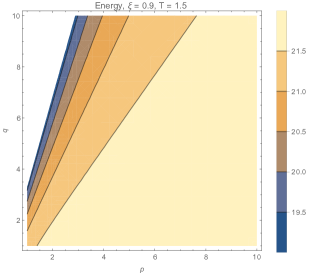
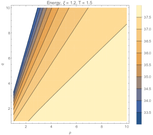
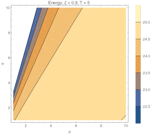
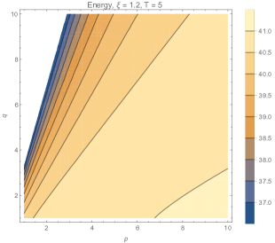
Figure 7: These plots exhibit the contour plot for the mean energy for different configurations of temperature and magnetic field. In those plots we can see the behavior of the Energy as a function of the wind numbers $(p,q)$.

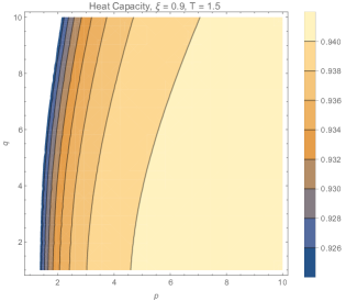
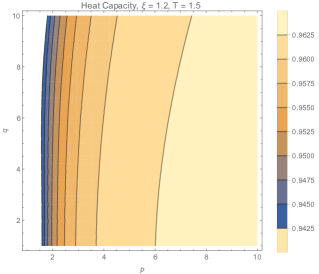
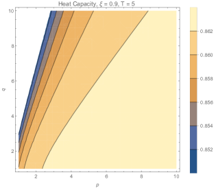
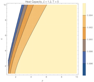
Figure 8: The contour plots for the Heat Capacity for different configurations of temperature and magnetic field. In these ones, we can see the behavior of the Heat Capacity as a function of the wind numbers $(p,q)$.

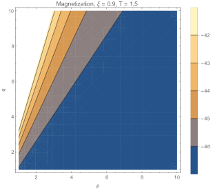
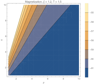
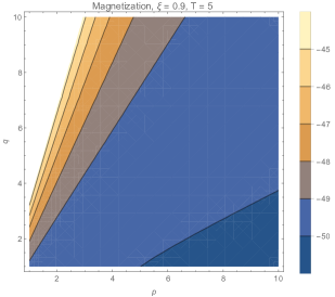
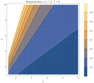
Figure 9: These contour plots show the magnetization for different configurations of temperature and magnetic field. In these ones, we can see the behavior of the magnetization as a function of the wind numbers $(p,q)$.

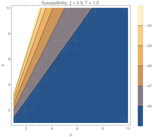
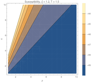
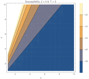
Figure 10: The contour plots show how the susceptibility varies for different configurations of temperature and magnetic field. In these plots, we see the behavior of the Susceptibility as a function of the wind numbers $(p,q)$.

II.1 Thin torus: the limit $a\rightarrow 0$

In this subsection, we focus on a particular case when the limit $a\rightarrow 0$ is taken into account. In other words, this means that we have a “circle” or a thin torus. Thereby, we get the following single particle partition function

$$\mathcal{Z}_{1}=\sqrt{\frac{\pi mp^{2}d^{2}}{2\beta}}\left\{1+\mathrm{erf}\left[-\frac{\xi}{4}\sqrt{\frac{2\beta}{m\left(1\right)}}\right]\right\}.$$ (21)

Using the same methodology, we can also get from the above result the Helmholtz free energy

$$f=-\frac{1}{\beta}\ln\sqrt{\frac{\pi mp^{2}d^{2}}{2\beta}}-\frac{1}{\beta}\ln\left\{1+\mathrm{erf}\left[-\frac{\xi}{4}\sqrt{\frac{2\beta}{m}}\right]\right\},$$ (22)

and the internal energy per particle

$$u = -\frac{1}{\beta^{2}}\left(\frac{1}{2}+\ln\sqrt{\frac{\pi mp^{2}d^{2}}{2\beta}}\right)-\frac{1}{\beta^{2}}\ln\left\{1+\mathrm{erf}\left(-\frac{\xi}{4}\sqrt{\frac{2\beta}{m}}\right)\right\}$$ (23)

$$\phantom{ss}-\frac{\xi}{\beta^{\frac{3}{2}}}\sqrt{\frac{1}{8m\pi}}\frac{\exp\left(-\frac{\xi^{2}}{8}\frac{\beta}{m}\right)}{1-\mathrm{erf}\left(\frac{\xi}{4}\sqrt{\frac{2\beta}{m}}\right)}.$$

The magnetization and susceptibility, respectively, are displayed below:

$$\mathfrak{m}=-\sqrt{\frac{1}{2\pi\beta m}}\frac{\exp\left(-\frac{\xi^{2}}{8}\frac{\beta}{m}\right)}{1-\mathrm{erf}\left(\frac{\xi}{4}\sqrt{\frac{2\beta}{m}}\right)},$$ (24)

$$\chi=-\frac{4}{\pi\beta}\frac{\mathcal{B}^{2}\exp\left(-2\mathcal{B}^{2}\xi^{2}\right)}{1-\mathrm{erf}\left(\mathcal{B}\xi\right)}\left\{\frac{1}{1-\mathrm{erf}\left(\mathcal{B}\xi\right)}-\sqrt{\pi}\mathcal{B}\xi\exp\left(\mathcal{B}^{2}\xi^{2}\right)\right\},$$ (25)

where the parameter $\mathcal{B}$ assumes the form:

$$\mathcal{B}=\frac{1}{4}\sqrt{\frac{2\beta}{m}}.$$ (26)

Let us now calculate the magnetization and the susceptibility for the same particular configuration of magnetic field and temperature as we did before. Initially, we consider a configuration in which $\xi=0$. For this case, we obtain the following results:

$$\mathfrak{m}_{\xi=0}=-\frac{1}{\sqrt{2\pi\beta m}},\phantom{aa}\chi_{\xi=0}=-\frac{1}{2\pi m}.$$ (27)

Now, for both $\xi=0$ and $T=0$, we get

$$\mathfrak{m}_{\xi=0,T=0}=0,\phantom{a}\chi_{\xi=0,T=0}=-\frac{1}{2\pi m}.$$ (28)

Here we notice that for $\xi=0$ and $T=0$, the magnetization turns out to be zero and we have a non-null constant susceptibility. On the other hand, considering the configuration where $\xi=0$, both magnetization and susceptibility are non-zero. We have to pay attention in the fact that the magnetization (when $\xi=0$) has the dependence on $T^{\frac{1}{2}}$. Another feature that is worth noticing is the fact that the mass ascribed to the fermions under consideration determines the magnitude of the susceptibility at zero magnetic field and also at zero temperature.

III Fermions on a torus knot

We intend now to apply the grand canonical ensemble approach to understand the behavior of $N$ noninteracting electrons moving in a prescribed torus knot on a single torus. Since this formalism takes into account the Fermi-Dirac statistics, we can obtain more information on how the Pauli principle can modify the properties of the system.

The grand partition function for the present problem reads

$$\Xi=\sum_{N=0}^{\infty}\exp\left(\beta\mu N\right)\mathcal{Z}\left[N_{\Omega}\right],$$ (29)

where $\mathcal{Z}\left[N_{\Omega}\right]$ is the canonical partition function which is now a function of the occupation number $N_{\Omega}$ and $\Omega$ label a quantum state. Since we are dealing with fermions, we know that the occupation number allowed for each quantum state is restricted to $N_{\Omega}=\left\{0,1\right\}$. So, for an arbitrary quantum state, the energy depends also on the occupation number as

$$E\left\{N_{\Omega}\right\}=\sum_{\left\{\Omega\right\}}N_{\Omega}E_{\Omega}$$

where we have the total fermion number $N$ defined as

$$\sum_{\left\{\Omega\right\}}N_{\Omega}=N.$$

Thus the partition function becomes

$$\mathcal{Z}\left[N_{\Omega}\right]=\sum_{\left\{N_{\Omega}\right\}}\exp\left[-\beta\sum_{\left\{\Omega\right\}}N_{\Omega}E_{\Omega}\right].$$ (30)

The grand partition function assumes the form

$$\Xi=\sum_{N=0}^{\infty}\exp\left(\beta\mu N\right)\sum_{\left\{N_{\Omega}\right\}}\exp\left[-\beta\sum_{\left\{\Omega\right\}}N_{\Omega}E_{\Omega}\right],$$ (31)

which can be rewritten as

$$\Xi=\prod_{\left\{\Omega\right\}}\left\{\sum_{\left\{N_{\Omega}\right\}}\exp\left[-\beta N_{\Omega}\left(E_{\Omega}-\mu\right)\right]\right\}.$$ (32)

Performing the sum over the possible occupation numbers, we obtain

$$\Xi=\prod_{\left\{\Omega\right\}}\left\{1+\exp\left[-\beta\left(E_{\Omega}-\mu\right)\right]\right\},$$ (33)

The connection with thermodynamics is made using the grand potential given by

$$\Phi=-\frac{1}{\beta}\ln\Xi.$$ (34)

Replacing $\Xi$ in the equation above, we get

$$\Phi=-\frac{1}{\beta}\sum_{\left\{\Omega\right\}}\ln\left\{1+\exp\left[-\beta\left(E_{\Omega}-\mu\right)\right]\right\}.$$ (35)

The entropy of the system can be cast in the following compact form, namely

$$S=-\frac{\partial\Phi}{\partial T}=-k_{B}\sum_{\left\{\Omega\right\}}\mathcal{N}_{\Omega}\ln\mathcal{N}_{\Omega}+\left(1-\mathcal{N}_{\Omega}\right)\ln\left(1-\mathcal{N}_{\Omega}\right)$$

where we explicitly use the Fermi-Dirac distribution function

$$\mathcal{N}_{\Omega}=\frac{1}{\exp\left[\beta\left(E_{\Omega}-\mu\right)\right]+1}.$$

We can also use the grand potential to calculate other important thermodynamics properties as mean particle number, energy, heat capacity and pressure using the following equation, respectively,

$$\mathcal{N}=-\frac{\partial\Phi}{\partial\mu},\phantom{ss}\mathcal{U}=-T^{2}\frac{\partial}{\partial T}\left(\frac{\Phi}{T}\right),\phantom{ss}C_{V}=T\frac{\partial S}{\partial T}.$$ (36)

we can also calculate, as before, the magnetization and the susceptibility.

In order to calculate all thermodynamics quantities described above, we need to perform before the sum present in Eq. $\left(\ref{eq:Gand-potential}\right)$. Fortunately, it is possible to do it in a closed form using again the Euler-MacLaurin formula. Before performing the sum, we will rewrite the energy $\left(\ref{q:SEnergy}\right)$ in a more convenient form

$$E_{n}=\frac{1}{2m}\frac{\hbar^{2}\left(1-\mathcal{A}\right)}{p^{2}d^{2}}\left[n+\frac{\xi}{\hbar}\frac{pd^{2}}{\left(1-\mathcal{A}\right)}\left(1-\mathcal{A}+\frac{\alpha^{2}}{2}\mathcal{A}\right)\right]^{2}-\frac{\xi^{2}\alpha^{4}\mathcal{A}^{2}d^{2}}{32m\left(1-\mathcal{A}\right)}.$$ (37)

Thereby, the grand partition function $\left(\ref{eq:Gand-potential}\right)\,\$can be rewritten as

$$\Phi=-\frac{2}{\beta}\int_{0}^{\infty}\mathrm{d}E\,\ln\left\{1+z\exp\left[-\beta E\left(n\right)\right]\right\}dn-\frac{1}{\beta}\ln\left\{1+ze^{-\beta\Upsilon}\right\},$$ (38)

where

$$\Upsilon\equiv\frac{\xi^{2}}{2m}\frac{d^{2}}{\left(1-\mathcal{A}\right)}\left(1-\mathcal{A}+\frac{\alpha^{2}}{2}\mathcal{A}\right)^{2}-\frac{\xi^{2}\alpha^{4}\mathcal{A}^{2}d^{2}}{32m\left(1-\mathcal{A}\right)}$$

Performing now the integration, we get

$$\Phi=\frac{\mathcal{L}}{\lambda}f_{\frac{3}{2}}\left(\Lambda,\mathfrak{X}\right)-f_{1}\left(\mathfrak{X}\right).$$ (39)

where $f_{\sigma}\left(\Lambda,\mathfrak{X}\right)$

$$f_{\sigma}\left(\Lambda,\mathfrak{X}\right)=\frac{1}{\Gamma\left(\sigma\right)}\int_{\Lambda}^{\infty}\frac{t^{\sigma-1}}{\mathfrak{X}^{-1}e^{t}+1}\mathrm{d}t,$$ (40)

is the incomplete Fermi-Dirac integral. We also define the quantities

$$\mathfrak{X} = ze^{\beta\Psi},$$ (41)

$$\Psi = \frac{\xi^{2}\alpha^{4}\mathcal{A}^{2}d^{2}}{32m\left(1-\mathcal{A}\right)},$$ (42)

$$\Lambda = \frac{\xi}{\hbar p}\frac{p^{2}d^{2}}{\left(1-\mathcal{A}\right)}\left(1-\mathcal{A}+\frac{\alpha^{2}}{2}\mathcal{A}\right),$$ (43)

$$\mathcal{L} = \frac{p^{2}d^{2}}{\left(1-\mathcal{A}\right)},$$ (44)

$$\lambda = \sqrt{\frac{2\pi\hbar^{2}}{m}\beta}.$$ (45)

For instance, the entropy is given by

$$S=\frac{\pi k_{B}\hbar^{2}}{m}\frac{\mathcal{L}}{\lambda^{3}}f_{\frac{3}{2}}\left(\Lambda,\mathfrak{X}\right)+k_{B}\left(\Psi+\mu\right)\frac{\mathcal{L}}{\lambda}f_{\frac{1}{2}}\left(\Lambda,\mathfrak{X}\right)-\frac{k_{B}\left(\Psi+\mu\right)ze^{-\beta\Upsilon}}{1+ze^{-\beta\Upsilon}}.$$ (46)

In order to give an idea of the behavior of the thermodynamic functions, we display below, in Fig. 11, 12 and 13, some plots taking into account the same values as those presented in Sec. II. Here, we see that for entropy, mean energy, heat capacity, and magnetization, when the temperature rises, the magnitude of their thermal properties increases; on the other hand, to the susceptibility the opposite behavior happened: when the temperature raised, the magnitude of such thermodynamic function decreased. On the other hand, when the magnetic field increases, the magnitude of entropy, mean energy and heat capacity decrease their values for a fixed temperature. However, the magnetization has an opposite behavior.

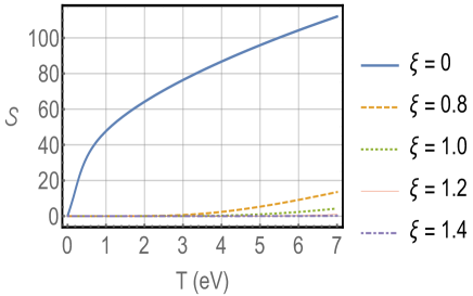
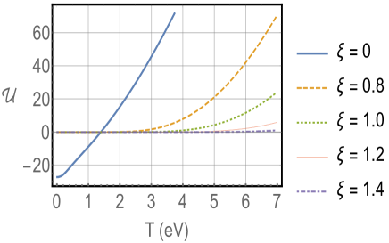
Figure 11: Entropy and internal energy

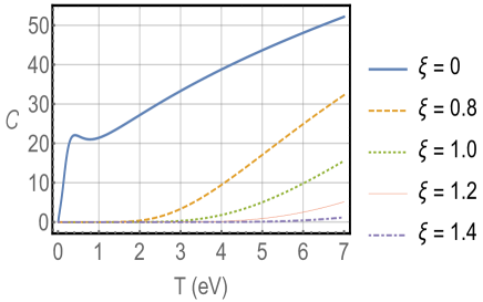
Figure 12: Heat capacity

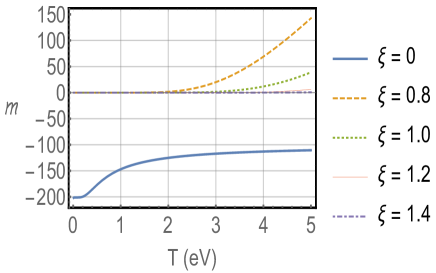
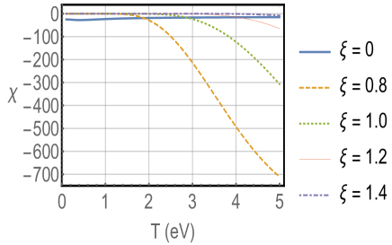
Figure 13: Magnetization and susceptibility

As an application, let us use the result obtained from the Eq. $\left(\ref{eq:GCanonicalFermion}\right)$ to probe how interaction affects the Fermi energy. From Eq. $\left(\ref{eq:GCanonicalFermion}\right)$ we get

$$N=g\left[\frac{\mathcal{L}}{\lambda}f_{\frac{1}{2}}\left(\Lambda,\mathfrak{X}\right)-\frac{\mathfrak{X}}{\mathfrak{X}+1}\right],$$ (47)

where $g$ is a weight factor that arises from the internal structure of the particles. The Fermi energy $\mu_{0}$ is the energy of the topmost filled level in the ground state of the $N$ electron system. In this way, we get

$$N=g\left\{\frac{4\mathcal{L}}{3}\left[\frac{m}{2\pi^{2}\hbar^{2}}\left(\Psi+\mu_{0}\right)\right]^{\frac{1}{2}}-1\right\}.$$ (48)

Solving the above equation for $\mu_{0}$, we get

$$\mu_{0}=\frac{9\pi^{2}\hbar^{2}}{8m\mathcal{L}^{2}}\left(\frac{N}{g}+1\right)^{2}-\Psi.$$ (49)

It is interesting to notice that the Fermi energy $\mu_{0}$ consists of two clearly divided parts. The first one contains the all information of a generic system; and all features of the specific torus (and torus-knot path) are encountered in the second part, $\Psi$. When we reduce the torus to a ring – when the limit $a\gg d$ is taken into account, we recover the well known result established in the literature dai2003quantum ; dai2004geometry .

IV Interacting Fermions on a Torus Knot

Following the interacting approach developed in [54], we can derive the modified grand canonical potential taking into account the interaction between fermions, namely

$$\Phi = -T\ln\mathcal{Z}$$ (50)

$$= -T\sum_{\Omega}\ln\left(1+\exp\left[-\beta\left(E_{\Omega}+u^{\prime}\left(\bar{n}\right)-\mu\right)\right]\right)+U\left(V,\bar{n}\right)-u^{\prime}\left(\bar{n}\right)\bar{N}.$$

The interaction is incorporated through $u^{\prime}\left(\bar{n}\right)$ term. Based on this equation, the other thermodynamic functions can be calculated as well. Performing as before the Euler-MacLaurin formula we find

$$\Phi=\frac{\mathcal{L}}{\lambda}f_{\frac{3}{2}}\left(\Lambda,\mathfrak{Z}\right)-f_{1}\left(\mathfrak{Z}\right)+U\left(V,\bar{n}\right)-u^{\prime}\left(\bar{n}\right)\bar{N}.$$ (51)

where we have now $\mathfrak{Z}=ze^{\beta\Psi}e^{-\beta u^{\prime}\left(\bar{n}\right)}$

So, the correction for the Fermi energy in this context is given by:

$$\mu_{0}=\frac{9\pi^{2}\hbar^{2}}{8m\mathcal{L}^{2}}\left(\frac{N}{g}+1\right)^{2}-\Psi+u^{\prime}\left(\bar{n}\right).$$ (52)

In contrast to the result derived in Eq. (49), the interaction term appears as an additional term in the above equation. However, notice that such expression is a generic one. Although we got an analytical result, we cannot proceed further unless the structure of the interaction term is explicitly introduced.

V Conclusion

This paper is aimed at investigating the topological effects on thermodynamic properties ascribed to a system of moving particles following a closed path through a torus knot. We exploited the grand canonical ensemble framework to study the system of noninteracting particles. Specifically, a fermionic system was studied. From an exact form of the partition function, analytic expressions of thermodynamic observables, e.g., Helmholtz free energy, the mean energy, the magnetization and the susceptibility, were obtained and their behavior for a range of parameter values and external conditions was graphically studied. In particular, we discussed in detail how topological features of the torus knot path affected the system. We also examined modifications of the Fermi energy. Finally, we outlined a procedure to introduce interaction in the fermionic sector. We hope that some of these characteristic features will be exhibited in near future in a real laboratory experiments, as we have indicated in this work.

References

- (1) D. R. Gaskell, Introduction to the Thermodynamics of Materials. CRC press, 2012.
- (2) B. Mühlschlegel, D. Scalapino, and R. Denton, “Thermodynamic properties of small superconducting particles,” Physical Review B, vol. 6, no. 5, p. 1767, 1972.
- (3) R. DeHoff, Thermodynamics in materials science. CRC Press, 2006.
- (4) R. Jones, “Thermodynamics and its applications–an overview,” 1974.
- (5) J. Davidovits, “Geopolymers: inorganic polymeric new materials,” Journal of Thermal Analysis and calorimetry, vol. 37, no. 8, pp. 1633–1656, 1991.
- (6) S. Safran, Statistical thermodynamics of surfaces, interfaces, and membranes. CRC Press, 2018.
- (7) F. S. Bates and G. H. Fredrickson, “Block copolymer thermodynamics: theory and experiment,” Annual review of physical chemistry, vol. 41, no. 1, pp. 525–557, 1990.
- (8) A. A. Araújo-Filho, F. L. Silva, A. Righi, M. B. da Silva, B. P. Silva, E. W. Caetano, and V. N. Freire, “Structural, electronic and optical properties of monoclinic na2ti3o7 from density functional theory calculations: A comparison with xrd and optical absorption measurements,” Journal of Solid State Chemistry, vol. 250, pp. 68–74, 2017.
- (9) F. L. R. e. Silva, A. A. A. Filho, M. B. da Silva, K. Balzuweit, J.-L. Bantignies, E. W. S. Caetano, R. L. Moreira, V. N. Freire, and A. Righi, “Polarized raman, ftir, and dft study of na2ti3o7 microcrystals,” Journal of Raman Spectroscopy, vol. 49, no. 3, pp. 538–548, 2018.
- (10) M. E. Casida, C. Jamorski, K. C. Casida, and D. R. Salahub, “Molecular excitation energies to high-lying bound states from time-dependent density-functional response theory: Characterization and correction of the time-dependent local density approximation ionization threshold,” The Journal of chemical physics, vol. 108, no. 11, pp. 4439–4449, 1998.
- (11) C. Lee, W. Yang, and R. G. Parr, “Development of the colle-salvetti correlation-energy formula into a functional of the electron density,” Physical review B, vol. 37, no. 2, p. 785, 1988.
- (12) M. Segall, P. J. Lindan, M. a. Probert, C. J. Pickard, P. J. Hasnip, S. Clark, and M. Payne, “First-principles simulation: ideas, illustrations and the castep code,” Journal of physics: condensed matter, vol. 14, no. 11, p. 2717, 2002.
- (13) J. P. Perdew and A. Zunger, “Self-interaction correction to density-functional approximations for many-electron systems,” Physical Review B, vol. 23, no. 10, p. 5048, 1981.
- (14) J. P. Perdew, “Density-functional approximation for the correlation energy of the inhomogeneous electron gas,” Physical Review B, vol. 33, no. 12, p. 8822, 1986.
- (15) J. P. Perdew and Y. Wang, “Accurate and simple analytic representation of the electron-gas correlation energy,” Physical review B, vol. 45, no. 23, p. 13244, 1992.
- (16) J. P. Perdew, K. Burke, and M. Ernzerhof, “Generalized gradient approximation made simple,” Physical review letters, vol. 77, no. 18, p. 3865, 1996.
- (17) W.-S. Dai and M. Xie, “Quantum statistics of ideal gases in confined space,” Physics Letters A, vol. 311, no. 4-5, pp. 340–346, 2003.
- (18) W.-S. Dai and M. Xie, “Geometry effects in confined space,” Physical Review E, vol. 70, no. 1, p. 016103, 2004.
- (19) H. Potempa and L. Schweitzer, “Dependence of critical level statistics on the sample shape,” Journal of Physics: Condensed Matter, vol. 10, no. 25, p. L431, 1998.
- (20) L. Angelani, L. Casetti, M. Pettini, G. Ruocco, and F. Zamponi, “Topology and phase transitions: From an exactly solvable model to a relation between topology and thermodynamics,” Physical Review E, vol. 71, no. 3, p. 036152, 2005.
- (21) M. P. Bendsoe and O. Sigmund, Topology optimization: theory, methods, and applications. Springer Science & Business Media, 2013.
- (22) R. Oliveira, A. Araujo Filho, R. Maluf, and C. Almeida, “The relativistic aharonov–bohm–coulomb system with position-dependent mass,” Journal of Physics A: Mathematical and Theoretical, vol. 53, no. 4, p. 045304, 2020.
- (23) P. Narang, C. A. Garcia, and C. Felser, “The topology of electronic band structures,” Nature Materials, vol. 20, no. 3, pp. 293–300, 2021.
- (24) L. D. Landau and E. M. Lifshitz, Course of theoretical physics. Elsevier, 2013.
- (25) L. E. Reichl, “A modern course in statistical physics,” 1999.
- (26) K. Huang, Introduction to statistical physics. CRC press, 2009.
- (27) N. Zettili, “Quantum mechanics: concepts and applications,” 2003.
- (28) E. M. Purcell, E. M. Purcell, E. M. Purcell, and E. M. Purcell, Electricity and magnetism, vol. 2. McGraw-Hill New York, 1965.
- (29) P. A. Tipler and R. Llewellyn, Modern physics. Macmillan, 2003.
- (30) H. Weyl, Gesammelte Abhandlungen: Band 1 bis 4, vol. 4. Springer-Verlag, 1968.
- (31) V. Sreedhar, “The classical and quantum mechanics of a particle on a knot,” Annals of Physics, vol. 359, pp. 20–30, 2015.
- (32) S. Ghosh, “Particle on a torus knot: Anholonomy and hannay angle,” International Journal of Geometric Methods in Modern Physics, vol. 15, no. 06, p. 1850097, 2018.
- (33) P. Das, S. Pramanik, and S. Ghosh, “Particle on a torus knot: Constrained dynamics and semi-classical quantization in a magnetic field,” Annals of Physics, vol. 374, pp. 67–83, 2016.
- (34) D. Biswas and S. Ghosh, “Quantum mechanics of a particle on a torus knot: Curvature and torsion effects,” EPL (Europhysics Letters), vol. 132, no. 1, p. 10004, 2020.
- (35) R. Da Costa, “Quantum mechanics of a constrained particle,” Physical Review A, vol. 23, no. 4, p. 1982, 1981.
- (36) Y.-L. Wang, M.-Y. Lai, F. Wang, H.-S. Zong, and Y.-F. Chen, “Geometric effects resulting from square and circular confinements for a particle constrained to a space curve,” Physical Review A, vol. 97, no. 4, p. 042108, 2018.
- (37) C. Ortix, “Quantum mechanics of a spin-orbit coupled electron constrained to a space curve,” Physical Review B, vol. 91, no. 24, p. 245412, 2015.
- (38) L. C. da Silva, C. C. Bastos, and F. G. Ribeiro, “Quantum mechanics of a constrained particle and the problem of prescribed geometry-induced potential,” Annals of Physics, vol. 379, pp. 13–33, 2017.
- (39) G. Ferrari and G. Cuoghi, “Schrödinger equation for a particle on a curved surface in an electric and magnetic field,” Physical review letters, vol. 100, no. 23, p. 230403, 2008.
- (40) L. W. Tu, “Manifolds,” in An Introduction to Manifolds, pp. 47–83, Springer, 2011.
- (41) L. W. Tu, Differential geometry: connections, curvature, and characteristic classes, vol. 275. Springer, 2017.
- (42) L. Liu, C. Jayanthi, and S. Wu, “Structural and electronic properties of a carbon nanotorus: Effects of delocalized and localized deformations,” Physical Review B, vol. 64, no. 3, p. 033412, 2001.
- (43) O. V. Kharissova, M. G. Castañón, and B. I. Kharisov, “Inorganic nanorings and nanotori: State of the art,” Journal of Materials Research, vol. 34, no. 24, pp. 3998–4010, 2019.
- (44) N. Chen, M. T. Lusk, A. C. Van Duin, and W. A. Goddard III, “Mechanical properties of connected carbon nanorings via molecular dynamics simulation,” Physical Review B, vol. 72, no. 8, p. 085416, 2005.
- (45) S. Madani and A. R. Ashrafi, “The energies of (3, 6)-fullerenes and nanotori,” Applied Mathematics Letters, vol. 25, no. 12, pp. 2365–2368, 2012.
- (46) Z. A. Lewicka, Y. Li, A. Bohloul, W. Y. William, and V. L. Colvin, “Nanorings and nanocrescents formed via shaped nanosphere lithography: a route toward large areas of infrared metamaterials,” Nanotechnology, vol. 24, no. 11, p. 115303, 2013.
- (47) H. Y. Feng, F. Luo, R. Kekesi, D. Granados, D. Meneses-Rodríguez, J. M. Garcia, A. García-Martín, G. Armelles, and A. Cebollada, “Magnetoplasmonic nanorings as novel architectures with tunable magneto-optical activity in wide wavelength ranges,” Advanced Optical Materials, vol. 2, no. 7, pp. 612–617, 2014.
- (48) L. Liu, G. Guo, C. Jayanthi, and S. Wu, “Colossal paramagnetic moments in metallic carbon nanotori,” Physical review letters, vol. 88, no. 21, p. 217206, 2002.
- (49) S. Vojkovic, A. S. Nunez, D. Altbir, and V. L. Carvalho-Santos, “Magnetization ground state and reversal modes of magnetic nanotori,” Journal of Applied Physics, vol. 120, no. 3, p. 033901, 2016.
- (50) J. Rodríguez-Manzo, F. Lopez-Urias, M. Terrones, and H. Terrones, “Magnetism in corrugated carbon nanotori: The importance of symmetry, defects, and negative curvature,” Nano Letters, vol. 4, no. 11, pp. 2179–2183, 2004.
- (51) H. Du, W. Zhang, and Y. Li, “Silicon nitride nanorings: Synthesis and optical properties,” Chemistry Letters, vol. 43, no. 8, pp. 1360–1362, 2014.
- (52) Y. Chan, B. J. Cox, and J. M. Hill, “Carbon nanotori as traps for atoms and ions,” Physica B: Condensed Matter, vol. 407, no. 17, pp. 3479–3483, 2012.
- (53) L. Peña-Parás, D. Maldonado-Cortés, O. V. Kharissova, K. I. Saldívar, L. Contreras, P. Arquieta, and B. Castaños, “Novel carbon nanotori additives for lubricants with superior anti-wear and extreme pressure properties,” Tribology International, vol. 131, pp. 488–495, 2019.
- (54) A. A. Araújo Filho and J. A. A. S. Reis, “Thermal aspects of interacting quantum gases in lorentz-violating scenarios,” The European Physical Journal Plus, vol. 136, no. 3, pp. 1–30, 2021.
- (55) J. Reis et al., “How does geometry affect quantum gases?,” arXiv preprint arXiv:2012.13613, 2020.
- (56) R. R. Oliveira, A. A. Araújo Filho, F. C. Lima, R. V. Maluf, and C. A. Almeida, “Thermodynamic properties of an aharonov-bohm quantum ring,” The European Physical Journal Plus, vol. 134, no. 10, p. 495, 2019.
- (57) R. Oliveira and A. A. Araújo Filho, “Thermodynamic properties of neutral dirac particles in the presence of an electromagnetic field,” The European Physical Journal Plus, vol. 135, no. 1, p. 99, 2020.
- (58) A. A. Araújo Filho and R. V. Maluf, “Thermodynamic properties in higher-derivative electrodynamics,” Brazilian Journal of Physics, vol. 51, no. 3, pp. 820–830, 2021.
- (59) A. A. Araújo Filho, “Lorentz-violating scenarios in a thermal reservoir,” The European Physical Journal Plus, vol. 136, no. 4, pp. 1–14, 2021.
- (60) A. A. Araújo Filho and A. Y. Petrov, “Higher-derivative lorentz-breaking dispersion relations: a thermal description,” The European Physical Journal C, vol. 81, no. 9, pp. 1–16, 2021.
- (61) A. A. Araújo Filho and A. Y. Petrov, “Bouncing universe in a heat bath,” International Journal of Modern Physics A, vol. 36, no. 34 & 35, (2021) 2150242. DOI: doi.org/10.1142/S0217751X21502420.
- (62) A. A. Araújo Filho, “Thermodynamics of massless particles in curved spacetime,” arXiv preprint arXiv:2201.00066, 2021.