Structure-Aware Feature Generation for Zero-Shot Learning

Abstract

Zero-Shot Learning (ZSL) targets at recognizing unseen categories by leveraging auxiliary information, such as attribute embedding. Despite the encouraging results achieved, prior ZSL approaches focus on improving the discriminant power of seen-class features, yet have largely overlooked the geometric structure of the samples and the prototypes. The subsequent attribute-based generative adversarial network (GAN), as a result, also neglects the topological information in sample generation and further yields inferior performances in classifying the visual features of unseen classes. In this paper, we introduce a novel structure-aware feature generation scheme, termed as SA-GAN, to explicitly account for the topological structure in learning both the latent space and the generative networks. Specifically, we introduce a constraint loss to preserve the initial geometric structure when learning a discriminative latent space, and carry out our GAN training with additional supervising signals from a structure-aware discriminator and a reconstruction module. The former supervision distinguishes fake and real samples based on their affinity to class prototypes, while the latter aims to reconstruct the original feature space from the generated latent space. This topology-preserving mechanism enables our method to significantly enhance the generalization capability on unseen-classes and consequently improve the classification performance. Experiments on four benchmarks demonstrate that the proposed approach consistently outperforms the state of the art. Our code can be found in the supplementary material and will also be made publicly available.

I Introduction

Zero-Shot Learning (ZSL) strives to recognize samples of unseen classes given their semantic descriptions, and have in recently years emerged as a widely-studied task due to their practical nature [1, 2, 3]. Typical ZSL approaches [4, 5, 6] tackles the problem by directly finding a shared latent space that aligns visual features and semantic embedding. However, learning such a shared space from the seen data have been found highly challenging, since the gap between the visual and semantic space is in many cases significant [7].

Figure 1: We quantitatively measure the average change of feature-prototype distance between the original visual space and the latent space on CUB dataste [8]. W-dist and L2-dist respectively denote Wasserstein distance and Euclidean distance. CLS denotes the classification loss, Center denotes the center constraint, and SP denotes the introduced structure-preserving constraint. A higher value indicates a greater change in geometric structure.

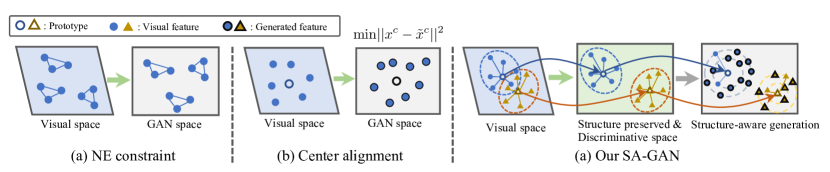
Figure 2: Comparison of different visual structure constraints for feature generation. (a) NE constraint [9] aims to maintain the neighbourhood structure between the visual and GAN space. (b) Center alignment [10] clusters fake samples to find visual centers and align the fake centers with the that of real ones. Here, $x^{c}$ and $\tilde{x}^{c}$ denote the class centers. (c) The proposed SA-GAN. Compared with existing methods, besides the difference in structure definition, our approach can better maintain the original structure information by using the mapped rather than the newly calculated prototype as a reference. Moreover, our method incorporates the prototype as condition input into the discriminator, which is more effective than adding a constraint loss to enforce the GAN to consider structure information. This is because the discriminator is usually the key to update the generator.

The works of [11, 12, 13] bypass learning such a direct visual-semantic alignment and resort to an alternative paradigm based on sample generation. They follow the workflow of first learning a sample generator conditioned on semantic embedding and then generating visual features of unseen classes for training the ZSL classifier. More recent works of [14, 10, 15] further improve this learning pipeline by introducing a mapping stage to enhance the feature quality, such as reducing redundancy [14] or increasing discriminability [15]. Though sample-generation-based approaches have demonstrated promising results, they still suffer from the issue that the generated samples for unseen-class are prone to collapsing to the seen-class centers.

In this paper, we look into the generalization capability of ZSL methods on unseen data, by explicitly incorporating the topological structure, defined as the geometry relationship between samples and their corresponding prototypes, into the learning of the latent space and the generator. The rationale behind this design lies in our experimental observation: without a topology-preserving constraint, the data topological structure change abruptly throughout the feature mapping, indicating that the model fails to capture the intrinsic data distribution and potentially leads to the bias towards the seen categories. We show some visual examples in Fig. 1

Specifically, our proposed scheme comprises two stages, structure-preserving mapping and structure-aware feature generation, as illustrated in Fig. 2(c). In the first stage, we impose a structure-preserving constraint in learning the mapping from visual features to the latent space. This constraint function aims to increase features’ discriminative power while penalizing any deviation to the original prototype structure. In the second stage, we enforce the GAN learning to handle the prototype structure, through utilizing additional supervision signals from a structure-aware discriminator and a feature reconstruction module. The discriminator is devised to distinguish fake samples from real ones conditioned on the corresponding prototype, while the reconstruction module ensures that the derived latent features may reconstruct the original ones.

We evaluate the proposed method on four challenging benchmark datasets under both the ZSL and the Generalized ZSL (GZSL) setting. Experimental results demonstrate that our approach significantly outperforms existing methods on most datasets under both settings. Our method achieves impressive performance on AWA2, CUB, SUN, and FLO datasets with harmonic mean accuracies of $68.0\%$, $58.7\%$, $44.4\%$ and $86.4\%$, respectively. Besides, using VAEGAN as a baseline, SA-GAN improves the unseen class recognition by 2.3%, 7.3%, 6.2%, and 28.2% on the above four datasets, validating the generalization capability of our method.

Our contribution is therefore a novel SA-GAN scheme that explicitly accounts for topological structure of samples throughout the ZSL pipeline, in which a structure-preserving constraint is imposed into the feature mapping and a structure-aware discriminator is introduced for the GAN to account for the sample distribution. SA-GAN delivers gratifying results consistently superior to the state of the art over four benchmarks, and significantly boosts the accuracy over unseen classes.

II Related Works

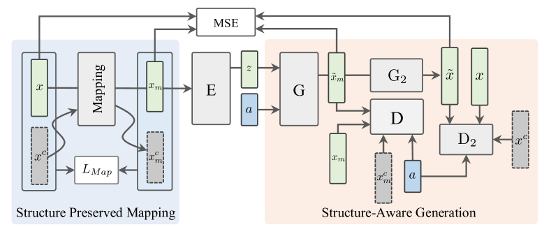
Figure 3: The framework of the proposed GZSL method. The latent feature $x_{m}$ is extracted by the mapping sub-network. The generator $G(\cdot)$ synthesizes new features $\tilde{x}_{m}$ based on class embedding $a$ and random noise $z$. The discriminator $D(\cdot)$ tries to distinguish between real and fake instances by measuring the relationship with the class embedding $a$ and prototype $x^{c}_{m}$. The second generator $G_{2}$ tries to recover the original visual features from the synthetic latent ones.

II-A Zero-Shot Learning

Zero-shot learning relies on the side information to exploit knowledge transferring from seen classes to a disjoint set of unseen classes. The side information can be class-level semantic descriptions or features, e.g., semantic attributes [16, 17, 18], and word vectors [19, 20] for bridging the gap between disjoint seen and unseen domain. Early researches focus on the conventional ZSL problem [21, 22, 5, 16, 23], which is dominated by the semantic embedding approaches [24, 5, 25, 26]. These methods learn to encode the visual features of seen class into the semantic spaces. For example, Socher et al. [22] learns a deep non-linear mapping between images and tags. Norouzi et al. [21] uses the probabilities of a softmax-output layer to weight the vectors of all the classes. Romera-Paredes et al. [25] proposes to learn visual-semantic mapping by optimizing a simple objective function with a closed-form solution. By doing so, the visual feature and the semantic embedding will share the same space, and the ZSL recognition can be accomplished by adopting the nearest neighbor classifier to assign given instances to corresponding classes or maximizing the compatibility score using various distance metrics. A well-trained ZSL model is then expected to maintain this ability in the unseen domain. Some works [27, 16, 5, 26] also attempt to learn an inverse mapping from the semantic vectors to the visual one. For example, DeViSE [5] learn a bilinear compatibility function using a multiclass with an efficient ranking formulation. Kodirov [26] uses an encoder to project the visual features into a semantic space and a decode to reconstruct the original visual space to preserve more information contained in the visual space.

Conventional ZSL tests only on the unseen classes, while the generalized zero-shot learning [28, 29, 30, 31, 32] is sparking more interest, where both seen and unseen classes are available in the inference stage. Since GZSL recognize the images from both seen and unseen classes, it is a more challenging task and suffers from a more serious data imbalance issue. Semantic embedding was developed for conventional ZSL fail to resolve this problem in GZSL. They tend to be highly overfitting the seen classes and harm the classification of unseen classes. This is verified by Xian et al. [29], where they conducted experiments and illustrated that almost all approaches designed for conventional ZSL see a significant drop in the GZSL setting.

Generative ZSL methods [11, 33, 34, 14, 15, 35] learn Generative Adversarial Networks (GANs) [36, 12, 15, 37] to synthesize unseen class features, thereby converting the ZSL problem to a supervised problem, then a ZSL classifier is learned for unseen class recognition. Among them, a typical generative method, f-CLSWGAN [11], uses Wasserstein GAN (WGAN) [38] to learn the generator for feature generation, which is achieved by optimizing a WGAN loss and a classification loss to ensure the feature discriminative power. The classifier can be replaced by an attribute regressor to guarantee the multi-modal cycle-consistency [12]. Another generative method, CADA-VAE [34] use two Variational Autoencoders (VAE) [39, 40] to align the visual feature and class embeddings in a shared latent space. By combining VAE and WGAN, Xian et al. [13] proposes f-VAEGAN, where GAN’s generator is used as a decoder of the VAE for feature generation. f-VAEGAN requires the decoder to reconstruct the visual feature, thereby promoting the cycle-consistency between generated and original visual features. Very recent works [14, 10, 15] seeks a two-stage pipeline, where the first stage projecting the visual feature to a latent space. The second stage follows the standard generative methods. These methods improve feature generation by integrating extra constraints to obtain a more appropriate latent space. For example, SARB [15] fine-tunes a pre-trained model with class embeddings to obtain a latent space that is discriminative and hubness-free. RFF-GZSL [14] restricts the mutual information between original visual features and the latest features so that the redundant information of original visual features can be removed without losing the discriminative information. Despite promising results demonstrated by these methods, they fail to consider the visual structure in learning the mapping and feature generator.

II-B Structure-Aware GAN.

There have been works [41, 42, 9] in the literature considering structure constraints in learning GAN networks. For example, PARTY [41] embeds local structure and prior sparsity information into the hidden representation learning to preserve the sparse reconstruction relation. Dist-GAN [42] uses latent-data distance constraint to enforce the compatibility between latent sample distance and the corresponding data sample distances, which alleviates the model collapse. GN-GAN [9] explores reversed t-SNE [43] to regularize the GAN training at both the local level and global level. In the context of ZSL, MCA [10] aligns semantic centers and visual centers in the source domain data and imposes this structure to the target domain data. Other works explore intra-class relations between prototypes and class samples, such as applying center loss [14, 44] to reduce intra-class variance and improve class discrimination. Wan et al. [10] also considers various metrics to align class centers between visual space and GAN space.

In this paper, we improve the GAN-based ZSL method by using a prototype structure. Our method is different from previous approaches as we consider the structure constraint in both mapping and feature generation. To the best of our knowledge, our method is the first to incorporate this kind of information in the two-stage ZSL recognition context. We systematically design a structure-preserving mapping module and structure-aware generation module that generates discriminative instances carrying structure information.

III Method

As shown in Fig. 3, our proposed learning framework mainly consists of two training stages: Structure-preserved mapping and structure-aware generation. The first stage aims to learn a mapping function that increases the feature discriminability while preserving the topological structure of data. After obtaining the mapped data from the previous step, we train a structural-aware generator using a discriminator incorporated with a prototype condition.

III-A Notation

In zero-shot learning, there is a set of images $X=\{x_{1},\cdots,x_{l}\}\cup\{x_{l+1},\cdots,x_{t}\}$ encoded in the visual space $\mathcal{X}$, a seen class label set $Y^{s}$, a unseen label set $Y^{u}$ and a class embedding set $A={a(y)|y\in{Y^{s}\cup Y^{u}}}$. $A$ is encoded in the semantic embedding space $\mathcal{A}$ that define the shared semantic relationship among categories. For example, two categories can be described by different combinations of a set of attributes. The first $l$ instances $x_{s}(x\leq l)$ are labeled as one of the seen classes $y_{s}\in Y^{s}$ while the other instances $x_{u}(l+1\leq n\leq t)$ belong to the unseen classes $y_{u}\in Y^{u}$. Using training set that contains only seen classes, the task of zero-shot learning is to predict the label of those unlabeled instances of unseen classes, i.e. $f_{zsl}\rightarrow\mathcal{Y}^{u}$. In generalized zero-shot learning, those unlabeled instances can be either from seen or unseen classes, i.e. $f_{gzsl}\rightarrow\mathcal{Y}^{s}\cup\mathcal{Y}^{u}$.

III-B Structure-Preserving Mapping

III-B1 Discriminative Mapping

In practice, the mapping function can be learned under the supervision of a classifier to ensure the discriminative power of the latent feature with the objective formulated as

$$L_{cls}=-\frac{1}{N_{s}}\sum^{N_{s}}_{i=1}H(y_{i},f_{c}({f_{m}({x_{i}})})$$ (1)

where $H$ is the cross entropy loss betwen true and predicted label of seen class instance $x_{i}$.

To further enhance the feature discriminativity we also use the center loss constraint which is proposde by Wen et al. [44],

$$L_{center}=\frac{1}{N_{s}}\sum^{m}_{i=1}||f_{m}(x_{i},m)-x^{c}_{m,y_{i}}||^{2}_{2}.$$ (2)

Among them, $x^{c}_{m,y_{i}}$ denotes the $y_{i}$th class center. It is initialized as a parameter to be updated in a mini-batch, and is jointly supervised by $L_{cls}$ and $L_{center}$. Together with classifier, the center loss greatly enhances the discriminative power of the learned feature $x_{m}$.

III-B2 Structure-Preserving Constraint

As discussed previously, directly learning a discriminative mapping will lead to losing the data’s structural information. In this section, we describe our proposed structural constraint to address this issue. We first define the structural information as the geometry relationship between samples and their corresponding prototypes. One naive way to measure the structural change after the mapping is to compute the class prototype separately in both original and mapped spaces, then compare the difference of each sample-prototype distance in both spaces. However, calculating the class prototype in each iteration is time-consuming make it infeasible in practice. Moreover, the new computed prototype (by averaging the same class’s mapped features) is usually different from the mapped prototype (by mapping the original prototype into the new space). To address these issues, we propose to directly use the mapped prototype to characterize the structural information in the new space. Therefore, our proposed structure-preserving constraint $L_{sp}$that penalizes the relative structure changes is expressed as:

$$L_{sp}=\frac{1}{N_{s}}\sum^{N_{s}}_{i}\Big{[}\lVert{x_{i}-x^{c}_{y_{i}}}\rVert_{2}-\lVert{f_{m}(x_{i})-f_{m}(x^{c}_{y_{i}})}\rVert_{2}\Big{]}^{2}$$ (3)

where the prototype, $x^{c}_{y_{i}}\in\mathbb{R}^{d_{s}}$, is the mean vector of the support instances sampled from the same class. The constant $l_{i}=\lVert{x_{i}-x^{c}_{y_{i}}}\rVert_{2}$ measures the $L_{2}$ distance between $x_{i}$ and its prototype $x^{c}_{y_{i}}$. $f_{m}$ is the mapping function. We simultaneously map the visual feature and its prototype onto the latent space and attempt to preserve their geometric distance which can be defined using any distance metrics such as Eucliden distance, cosine similariy, et al.

III-B3 Mapping Objective

The classifier, center-loss, and structure-preserving constraint are learned simultaneously by joint minimizing the loss function represented in equation 1, 2, and 3 weighted by the factor $\gamma_{c}$ and $\gamma_{s}$.

$$L_{Map}=L_{cls}+\gamma_{c}L_{center}+\gamma_{s}L_{sp},$$ (4)

where $\gamma_{c}$ and $\gamma_{s}$ are set to 0.01 and 1.0 in this paper. $L_{cls}$ and $L_{c}$ ensure that the latent feature is discriminative to benefit category recognition. The former two focuses on separability of the seen classes by the other information such as prototype structure are not considered. This issue is addressed by the prototype structure constraint $L_{sp}$.

At the end of stage 1, the visual feature in the new space can implicitly encode structural information within discriminative representations. Therefore, it not only enjoyes discriminative power but also retain a high-quality structure. The mapping function carrying these characteristics provides a well-generalized space for subsequent GAN learning.

III-C Structure-Aware Feature Generation

III-C1 Mapped GAN

In the second stage, we aim to encourage the generator to produce discriminative and structure-aware features in latent space. We achieve this by modifying the discriminator to include class prototypes as an auxiliary input to train the conditional generator. It is then optimized by a Wasserstein adversarial loss defined by

$$\begin{split}L_{mWGAN}&=\mathbb{E}[D(x_{m},a_{y},x^{c}_{m,y};\;\theta_{D})]\\ &-\mathbb{E}[D(\tilde{x}_{m},a_{y},x^{c}_{m,y};\;\theta_{D})]\\ &-\lambda\mathbb{E}[(||\triangledown_{\hat{x}_{m}}D(\hat{x}_{m};\;\theta_{D})||_{2}-1)^{2}]\end{split}$$ (5)

where $G(\cdot|\theta_{G})$ is the generator, $D(\cdot|\theta_{D})$ denote the discriminator. The generator synthesizes instances $\tilde{x}_{m}=G(z,a_{y})$ conditioning on class embedding $a$ and a multi-dimension Gaussian distribution $z\sim\mathcal{N}(0,1)$. Besides, $\hat{x}_{m}=\alpha x_{m}+(1-\alpha)\tilde{x}_{m}$ where $\alpha\sim U(0,1)$, and $\lambda$ is the penalty coefficient.

III-C2 Reconstructed GAN

Note that SA-GAN generates visual features in the structured-preserved latent space, but does not guarantee that the generated features are well fitted to the visual distribution, which might lead to ineffective learning of the final linear classifier. We conjecture that this issue could be alleviated by reconstructing the original feature space from the mapped space. To this end, we optimize a second GAN sub-network

$$\begin{split}L_{rWGAN}&=\mathbb{E}[D_{2}(x,a_{y},x^{c}_{y};\;\theta_{D_{2}})]-\mathbb{E}[D_{2}(\tilde{x},a_{y},x^{c}_{y};\;\theta_{D_{2}})]\\ &-\lambda\mathbb{E}[(||\triangledown_{\hat{x}}D_{2}(\hat{x};\;\theta_{D_{2}})||_{2}-1)^{2}]\end{split}$$ (6)

where $\tilde{x}=G_{2}(x_{m},a_{y})$, $\hat{x}=\alpha x+(1-\alpha)\tilde{x}$ with $\alpha\sim U(0,1)$, and $\lambda$ is the penalty coefficient. Minimizing the $L_{rWGAN}$ requires a high-quality recovery and rich information encoded in the generated features. $L_{rWGAN}$ also enforces cycle-consistency on feature embeddings between latent space and original visual space.

III-C3 Objective

The structure-aware generation can be fused into WGAN and VAEGAN, referred to as SA-WGAN and SA-VAEGAN. Among them, SA-VAEGAN includes an encoder $E(\cdot)$ to map visual instance to a latent variable $z$. The decoder/generator takes $z$ as input and tries to recover the visual feature. Specifically, the VAE objective contains a KL (Kullback-Leibler divergence) and a reconstruction loss. Using MSE (mean square error) as the reconstruction loss, the VAE loss is formulated as

$$\begin{split}L_{VAE}&=\text{KL}(E(x_{m})||p(z))+\mathbb{E}[\text{MSE}(G(z,a),x_{m})]\\ &+\mathbb{E}[\text{MSE}(G_{2}(x_{m}),x)],\end{split}$$ (7)

The overall objective function of SA-VAEGAN in the second stage is defined by

$$L_{SA-VAEGAN}=L_{VAE}+\gamma_{m}L_{mWGAN}+\gamma_{r}L_{rWGAN},$$ (8)

where $\gamma_{r}$ is used to balance learning of the second generator and is set to 0.1 in this paper. $\gamma_{m}$ is set to 1. The objective of SA-WGAN contains only last two items.

TABLE I: Statistics of five benchmark datasets used in the experiments, in terms of class embedding dimensions $K_{a}$, number of seen classes $Y_{s}$, number of unseen classes $Y_{u}$, number of training samples $X^{tr}$, numbers of test seen instances $X^{te}_{s}$ and unseen instances $X^{te}_{u}$.

Dataset	$K_{a}$	$Y_{s}$	$Y_{u}$	$X^{tr}$	$X^{te}_{s}$	$X^{te}_{u}$
AWA2	85	40	10	23,527	7,913	5,882
CUB	312	150	50	7,075	2,967	1,764
SUN	102	580	65	14,340	1,440	2,580
FLO	1,024	82	20	1,640	5,394	1,155

Give the learned generator $G$, we synthesize unseen instances by inputting corresponding class embedding $a$ and noise $z$. The generated unseen instances and real seen instances are then used to learn a linear classifier for final classification.

In this paper, we use the prototype-instance relationship to characterize the intrinsic data structure required to preserving during the mapping stage, which requires us to use the class prototype. In the feature generation stage, existing ZSL methods learn discriminator by measuring the relationship between instance, while the prototype enables us to handle structure information which serves as an additional supervision signal to enhance the discriminator learning as well as improving the generalizability of the generator. In addition, as illustrated in Fig. 2 in the paper, compared with other feature structures such as neighborhood structures, the prototype is easier to compute. Once obtained, the class prototype can be flexibly applied to mapping sub-network and GAN sub-network without re-computation in each iteration.

TABLE II: Comparing the proposed method with state-of-the-art methods on four benchmarks. We report average per-class top-1 accuracy for unseen (U) classes and seen (S) classes and their harmonic mean (H) in percentage. The best results are highlighted.

Method	Zero-Shot Learning			Generalized Zero-Shot Learning
	CUB	SUN	FLO	AWA2			CUB			SUN			FLO
	T1	T1	T1	U	S	H	U	S	H	U	S	H	U	S	H
f-CLSWGAN [11]	57.3	-	67.2	-	-	-	43.7	57.7	49.7	42.6	36.6	39.4	59.0	73.8	65.6
Cycle-WGAN [12]	58.6	-	70.3	-	-	-	45.7	61.0	52.3	49.4	33.6	40.0	59.2	72.5	65.1
SE-ZSL [45]	59.6	63.4	-	58.3	68.1	62.8	41.5	53.3	46.7	40.9	30.5	34.9	-	-	-
f-VAEGAN [13]	61.0	64.7	67.7	57.1	76.1	65.2	48.4	60.1	53.6	45.1	38.0	41.3	56.8	74.9	64.6
SARB-I [15]	63.9	62.8	-	30.3	93.9	46.9	55.0	58.7	56.8	50.7	35.1	41.5	-	-	-
CADA-VAE [34]	60.4	-	-	55.8	75.0	63.9	51.6	53.5	52.4	47.2	35.7	40.6	-	-	-
GMN [37]	64.3	63.6	-	-	-	-	56.1	54.3	55.2	53.2	33.0	40.7	-	-	-
LisGAN [46]	58.8	-	69.6	-	-	-	46.5	57.9	51.6	42.9	37.8	40.2	57.7	83.8	68.3
ABP [47]	58.5	-	-	55.3	72.6	62.6	47.0	54.8	50.6	45.3	36.8	40.6	-	-	-
TCN [48]	59.5	61.5	-	61.2	65.8	63.4	52.6	52.0	52.3	31.2	37.3	34.0	-	-	-
GXE [49]	54.4	62.6	-	56.4	81.4	66.7	47.4	47.6	47.5	36.3	42.8	39.3	-	-	-
RFF [14]	-	-		-	-	-	52.6	56.6	54.6	45.7	38.6	41.9	65.2	78.2	71.1
OCD [50]	60.3	63.5	-	59.5	73.4	65.7	44.8	59.9	51.3	44.8	42.9	43.8	-	-	-
DEVB [51]	-	-	-	63.6	70.8	67.0	53.2	60.2	56.5	45.0	37.2	40.7	-	-	-
TF-VAEGAN [52]	64.9	66.0	70.8	59.8	75.1	66.6	52.8	64.7	58.1	45.6	40.7	43.0	62.5	84.1	71.7
SA-WGAN	62.4	63.7	80.9	59.7	73.2	65.8	53.8	61.6	57.4	47.6	40.9	44.0	77.1	88.4	82.4
SA-VAEGAN	64.5	64.4	89.3	59.4	79.5	68.0	55.7	62.0	58.7	51.3	39.1	44.4	85.0	87.7	86.4

IV Experiments

In this section, we first describe the benchmarks, implementation details, and evaluation protocols. We then report the results of our method based on both WGAN and VAEGAN, and compare them with state-of-the-art ZSL/GZSL approaches. After that, we conduct ablation studies to investigate the effectiveness of our method.

IV-A Dataset

We validate the proposed method on four commonly used ZSL/GZSL datasets, which are Animals with Attributes 2 (AWA2) [29], CUB-200-2011 (CUB) [8], SUN with Attributes (SUN) [53], Oxford Flowers (FLO) [54]. Among them, CUB and FLO are fine-grained datasets, and the other two are coarse-grained datasets. The semantic labels used by the datasets are provided by the category attributes. For fair comparison against existing approaches, the split of seen/unseen classes follows the newly proposed setting (PS) [29], which strictly separates the training classes from the pre-trained model. For FLO, we use the standard split and sentence-based semantic descriptions provided by Reed et al. [55]. We list the statistics of these datasets in Table I.

TABLE III: Classification accuracy (%) of conventional zero-shot learning for standard split (SS). The best results are highlighted.

Method	CUB	AWA2	SUN
CONSE[21]	36.7	67.9	44.2
SSE [56]	43.7	67.5	54.5
LATEM [57]	49.4	68.7	56.9
ALE[27]	53.2	80.3	59.1
DEVISE[5]	53.2	68.6	57.5
SJE[16]	55.3	69.5	57.1
ESZSL[25]	55.1	75.6	57.3
SYNC[58]	54.1	71.2	59.1
SAE[26]	33.4	80.2	42.4
GFZSL[59]	53.0	79.3	62.9
SE-ZSL[45]	60.3	80.8	64.5
DCN[60]	55.6	-	67.4
OCD[50]	60.8	81.7	68.9
SA-WGAN	66.7	82.1	66.6
SA-VAEGAN	67.5	82.2	67.1

IV-B Implementation Details

Throughout the paper, visual features are extracted from the image with 2048-dim using ResNet-101 [61] extractor. There is no pre-processing technique used in the feature extraction. Specifically, the ResNet-101 model is pre-trained on ImageNet 1K without fine-tuning. Similar to [11, 12], for FLO, we extract 1024-dim character-based CNN-RNN [55] features that encode the text description of the image containing the fine-grained visual descriptions (10 sentences per image). There is no interaction between seen and unseen sentences during CNN-RNN training. In this case, the per-class sentences are build by averaging the CNN-RNN features of the same class. Note that for FLO, all methods except DeViSE [5] use the RNN-CNN description [55].

We have formally defined the objective function and depicted the framework in Fig. 3. The encoder $E$, generator $G$, $G_{2}$, discriminator $D$, $D_{2}$ are implemented as multiple-layer perceptron (MLP) with a single hidden layer containing 4096 nodes and LeakyReLU [62] as the activation function. We use Adam optimizer with $\beta_{1}=0.5$, $\beta_{2}=0.999$ for both stages. The batch sizes for mapping network and GAN training are 256 and 64. We train 100 epochs in the mapping sub-network and 1000 epochs for the learning of feature generation. For all datasets, we uniformly set the learning rate to 1e-4.

IV-C Evaluation Protocols

For evaluation protocols, we follow the protocol proposed in [29] to evaluate ZSL and GZSL performance. In particular, we average the correct predictions for each class and report the top-1 accuracy of per class. For conventional ZSL setting, the evaluation metric is defined as follows,

$$MCA_{u}=\frac{1}{|U|}\sum_{y^{u}\in{U}}acc_{y^{u}}$$ (9)

where $acc_{y^{u}}$ denotes the top-1 accuracy on the unseen test data for each class in the unseen domain $U$. The $|U|$ denotes the class number.

In the generalized ZSL setting, we compute the averaget per class top accuracy for both seen and unseen classes and report the harmonic mean of seen and unseen accuracy. The GZSL evaluation protocal is computed as follows,

$$H=\frac{2*MCA_{s}*MCA_{u}}{MCA_{s}+MCA_{u}}$$ (10)

where $MCA_{u}$,$MCA_{s}$ denote the mean class accuracy on unseen and seen classes respectively. A well-trained GZSL model is required to reach good results on the unseen domain while maintaining the recognition capability in the seen domain. A higher harmonic mean indicates a better balance between seen classes and unseen classes.

IV-D Comparing with the State-of-the-Art

IV-D1 Conventional ZSL Using Standard Splits

Table III summarizes the results of conventional zero-shot learning on AWA2, CUB and SUN datasets. These results are obtained from Xian et al. [63, 29] using standard split (SS) with ResNet-101 as the feature extractor. From the table, we can see that the classification accuracy obtained on the SS protocol on AWA2, CUB, and SUN datasets are 82.2%, 67.5%, 67.1%, respectively. SA-GAN does not outperforms all the prior approaches on all dataset for the inductive setting. However, compared with the best existing methods, our method illustrates a significant advantage on the CUB dataset with around 7% improvement. In addition, we achieve consistent improvement on the AWA2 dataset with 0.5% improvement. The result on SUN is also competitive with an accuracy of 67.1%. Although OCD obtains better results on SUN, the results of SA-GAN on the other two datasets are higher with improvents of 6.7% and 0.5% respectively. We attribute this performance gain to the increased discriminitive power by the mapping sub-nework with .

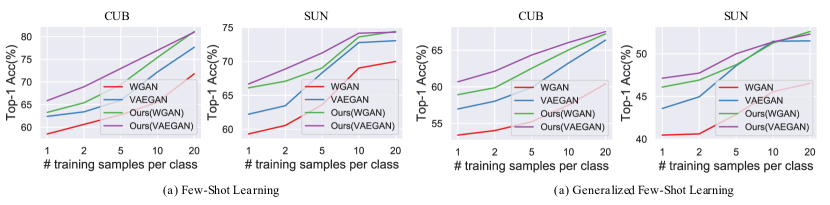
Figure 4: FSL and GFSL results on CUB and SUN with increasing number of training samples per novel class.

TABLE IV: Zero-shot learning using fine-tuned feature on CUB, AWA2 and SUN datasets.

Method	Zero-Shot Learning			Generalized Zero-Shot Learning
	AWA2	CUB	SUN	AWA2			CUB			SUN
	T1	T1	T1	U	S	H	U	S	H	U	S	H
SBAR-I [15]	65.2	63.9	62.8	30.3	93.9	46.9	55.0	58.7	56.8	50.7	35.1	41.5
f-VAEGAN [13]	70.3	72.9	65.6	57.1	76.1	65.2	63.2	75.6	68.9	50.1	37.8	43.1
TF-VAEGAN [52]	73.4	74.3	66.7	55.5	83.6	66.7	63.8	79.3	70.7	41.8	51.9	46.3
SA-WGAN	68.1	71.3	63.5	80.6	62.1	70.2	73.7	63.5	68.2	43.3	49.5	46.2
SA-VAEGAN	70.5	72.3	63.5	82.3	63.9	71.9	75.7	65.4	70.2	49.9	43.7	46.7

IV-D2 ZSL/GZSL Setting using Proposed Splits

Table II compares our method with state-of-art methods proposed recently on four zero-shot learning datasets under both ZSL and GZSL settings using proposed split (PS) et al. without fine-tuning the feature extractor on the target datasets. [63, 29]. SA-GAN improves over f-CLSWGAN [11], Cycle-WGAN [12], SE-ZSL [45], f-VAEGAN [13], SARB-I [15], CADA-VAE [34], GMN [37], LisGAN [46], ABP [47], TCN [48], GXE [49], RFF [14], OCD [50], DEVB [51] and TF-VAEGAN [52] over all the benchmarks measured by harmonic mean. Those prior methods utilized the semantic space for class embedding without considering the topological structure in the sample generation and thus restricted by the generalization problem. We observe that SA-GAN achieves new state-of-art results, i.e., 68.0% on AWA2, 58.7% on CUB, 44.4% on SUN, and 86.4% on FLO, which are 4.5%, 5.1%, 3.1%, and 21.8% improvements from VAEGAN baseline. This is because SA-GAN not only promotes the feature discriminative power in the mapping space like SABR-I but also preserves the hidden structure information characterized by the instance-prototype relationship in the mapping stage and the feature generation stage. A similar result can be seen when we compare SA-GAN with f-CLSWGAN. Concretely, SA-GAN improves the results by 7.7%, 5.0%, and 20.8% on CUB, SUN, and FLO respectively. Note that SA-GAN using a mapping subnetwork in a two-stage scheme like SABR-I, but obtains better results improving the results by 21.1%, 1.9%, 2.9% on AWA2, CUB, and SUN. This is because SABR-I uses an additional mapping sub-subnetwork to address the hubness problem. However, projecting the visual feature by the classifier and semantic alignment reduces the bias of the seen classes at the cost of deconstructing the structure information embedded in the visual space.

Most existing G/ZSL approaches performs well on the seen domain but fail to achieve satisfying results for unseen classes, even through they are try to addres the isuue, which indicates that a large biases towards seen classes is challenging in the ZSL field. Our model mitigate the gap between seen and unseen classes, as shown in Table II. With the structure-preserved mapping and structure-aware generator, the $MCA_{u}$ increases and a better balance between the accuracy of seen and unseen classes is obtained. Therefore, our generative-based approaches competitively benefit the zero-shot learning in the realistic and challenging task. This also partially explain why there are a few unpromising result in the Table II and Table III. Although not state-of-art on the unseen split, our method cares more about the overall performance where both seen and unseen classes are included for prediction.

IV-E (Generalized) Few-shot Learning

In few-shot learning, the data classes are split into base classes containing a large number of training data and novel classes that contain few labeled examples each class. A good few-shot model is required to achieve good results on novel classes. Similar to GZSL, the generalized few-shot learning measure the performance across all classes. Following f-VAEGAN, we use the same split as (G)ZSL, i.e. 150 base classes and 50 novel classes on CUB. However, there is no training data available for novel classes in ZSL, since all data of novel classes from the original dataset are combined for ZSL evaluation. To enable few-shot learning, we split the novel data into training/test according to the protocol in the original dataset. We use the base class data as the support set. During training, we randomly sample (1, 2, 5, 10, 20) instances, and combine them with support data for model learning. Other settings remain the same as (G)ZSL. In the test time, we report top-1 accuracy in both few-shot and generalized few-shot learning.

TABLE V: Contribution of components to the generalized zeroshot learning (H) on the CUB dataset. SP-Map denotes structure-preserving mapping, mWGAN denotes structure-aware feature generation in the mapped space, and rWGAN reconstructs original visual features from latent ones.

Baseline	SP-MAP	mWGAN	rWGAN	ZSL	U	S	H
✓				56.81	48.15	56.68	52.06
✓	✓			62.03	52.89	60.26	56.34
✓		✓		63.05	53.51	60.51	56.80
✓	✓	✓		64.04	54.04	62.99	58.17
✓	✓	✓	✓	64.48	56.39	61.31	58.74

Fig. 4 shows that the results obtained by our method significantly improves over the GZSL setting even only using a few labeled real instances. Specifically, compared with ZSL, one-shot learning uses one labelled real instance for each novel class and improve the accuracy by 10%. The accuracy improvements from 1 to 20 shots is over 15%. Besides, while the top-1 accuracy increases with the number of shots for all compared methods, our method outperforms the baseline by a large margin in both few-shot and generalized few-shot learning, which indicates a strong generalization ability of our method.

IV-F Ablation Studies

In this section, we study the properties of the proposed method by conducting a series of ablation experiments, including the target feature dimension, number of synthetic samples.

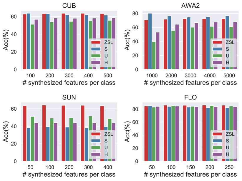
Figure 5: Impact of the number of synthetic instances on the CUB dataset.

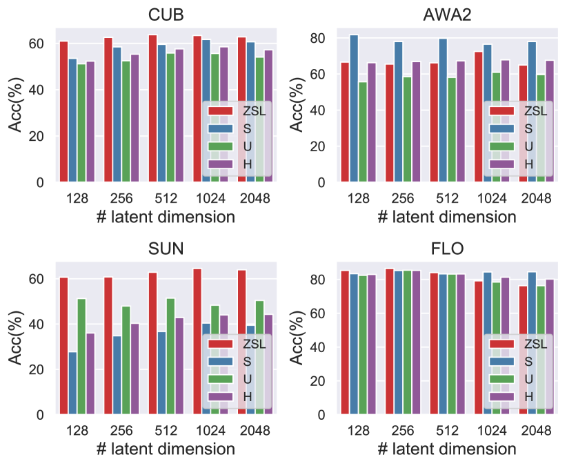
Figure 6: Impact of the latent dimension in terms of ZSL, U, S, H on four datasets.

Figure 7: Comparing VAEGAN and SA-VAEGAN using t-SNE embeddings of the generated feature on CUB and SUN. The top row illustrates VAEGAN, and the bottom row shows our method. The symbol $\bullet$ denotes the instance of seen classes, and $\mathbf{\times}$ denotes the instance of unseen classes.

IV-F1 ZSL on Fine-Tuned Feature

We also evaluate our method using fine-tuned features on three datasets in Fig. IV. Overall, the improvement is significant when compared with approaches without using fine-tuned features. Compared with the methods using the fine-tuned features, our method also illustrates the consistent improvement in GZSL on two datasets.

IV-F2 Metric of Instance-Prototye Measurement

Note that, throughout the papaer we use L2 distance as the metric to evaluate the relationship between instance and its class prototypes. Here we conduct experiments to test the model performace under different distnace metrics including L1, L2, and cosine distance and record the results in Table VI The results show that L2 distance is more effective for the model to achieve a higher performance.

TABLE VI: Results comparison of different distance metrics on the cub dataset.

	ZSL	U	S	H
L1	62.81	52.04	60.64	56.01
Cosine	62.77	54.30	61.95	57.87
L2	64.54	56.53	61.41	58.87

IV-F3 Impact of Model Components

SA-GAN has utilized multiple techniques to improve the performance. We evaluate the effectiveness of components used in SA-VAEGAN. Table V summarizes the results of four settings. The baseline model consists of a generator $G$, a discriminator $D$, and an encoder $E$. Based on the baseline, we evaluate the model performance by introducing structure-preserving mapping (SP-Map), mapped GAN (mWGAN), and reconstructed GAN (rWGAN). We report harmonic mean (H) on the CUB dataset. Table V shows significant improvement over the VAEGAN method. The complete version gives the highest results, achieving a whopping accuracy gain of 6.6%. Specifically, the introduced structure-preserving mapping remarkably enhances the harmonic mean by a large margin (4.7%). This is because the SP-Map not only promotes feature discriminative power but retains prototype structure for high-quality mapping. After utilizing the mWGAN, the model performance takes a further enhancement. The baseline discriminator measures the relation of an instance and its class embedding but mWGAN further includes prototypes, which considers more structural information. By combining these modules, our method yields the best results.

Table VII further shows the result comparison between using and without using structure-preserving loss. From the table, we can see that the structure-preserving loss improves the model performance in terms of all metrics, which confirms the effectiveness of structure-preserving loss.

TABLE VII: Results comparison with/without Structure-Preserving (SP) loss on the CUB dataset.

	ZSL	U	S	H
without SP	63.27	55.82	58.79	57.26
with SP	64.54	56.53	61.41	58.87

Note that the visual features are extracted by the ImageNet pre-trained network. The extracted feature with a high dimension contains redundant information. By using a mapping network, we can project the visual feature to a compact space to reduce the influence of redundant information. The mapping network with pre-defined constraints can also endow the mapped features with new properties such as increased discriminative power by the classification loss and center loss constraint, making the new features more task-specific. In this paper, we also encode structural information within the mapped feature by the proposed structure-preserving constraint. Our experiments show that the mapping sub-network improves the model generalizability and benefit the zero-shot recognition.

Existing works enforce a cycle-consistency between visual features and semantic embeddings. The proposed reconstructed GAN enables a cycle consistency between the mapping space and the original visual space. In the ablation study, we verify the effectiveness of the reconstructed GAN in Table V in the paper. More detailed results are also illustrated in Table 1 in the supplementary materials. These experiments show that the reconstructed GAN further improves the model performance by over 0.5%.

IV-F4 Impact of Synthetic Numbers

We show in Fig. 5 results of our method under different numbers of synthesized instances of unseen classes on four datasets. In general, the performance remains stable across benchmarks. When the amount of synthesized instances is small, unseen classes’ accuracy is low (ZSL, U, H). This is because insufficient unseen class data causes data imbalance problem, encouraging the GZSL classifier to be more focused on learning from seen class data. The issue is alleviated when the amount increases. As a result, the ZSL, U, and H results improve rapidly. Besides, to address the imbalanced problem, the fine-grained dataset usually required a smaller number of synthetic instances before achieving the best performance, while for coarse-grained dataset, the optimal number is larger.

IV-F5 Impact of the Latent Dimension

The effect of the latent dimension of the hidden feature, evaluated by the proposed method, is illustrated in Fig. 6. In general, when the dimension is low, the performance is poor. One reason is that the very low feature dimension is not enough to fully describe the target class. As the dimension increases, the unseen accuracy and harmonic mean gain consistent improvement, and when the dimension exceeds a certain threshold, the performance does not improve. We use 1,024 as the mapped dimension throughout this paper because our method has already achieved good results on the selected datasets.

IV-F6 Feature Visualization

Figure 8: Model performances on the CUB dataset with different coefficients

In Fig. 7, we provide statistics to compare SA-VAEGAN with VAEGAN in terms of the synthetic features on the CUB dataset. We selected the ten unseen classes and ten seen classes for T-SNE [43] visualization. As shown in Fig. 7, there are overlapping among unseen classes for VAEGAN. However, our method leads to more visible clusters, where the synthesized samples of the selected category become more compact. The synthesized features are more discriminative, and those overlapped classes become more separable. This proves that the SA-GAN is powerful in generating more discriminative features for unseen classes.

IV-G Analysis of Loss Coefficients

We study the effect of loss coefficients $\gamma_{s}$, $\gamma_{c}$, $\gamma_{w}$, $\gamma_{r}$ to obtain a more intuitive observation on the module influence in Fig. 8. These experiments are all conducted on the CUB dataset. $\gamma_{s}$ controls the importance of structure-preserving, $\gamma_{c}$ controls the importance of features’ discriminative power, $\gamma_{m}$ controls the importance of GAN, while $\gamma_{r}$ controls the importance of visual feature recovery. These figures show that the model performance remains stable when the loss coefficients $\gamma_{s}$, $\gamma_{m}$, $\gamma_{r}$ are small. However, the performance decreases dramatically when these coefficients become very large. Besides, different coefficients have different best values. For $\gamma_{c}$, the harmonic mean achieves the best performance at 0.01. This is because the center loss can promote the features’ discriminative power, and when $\gamma_{c}$ is low, the features are not discriminative enough to benefit model performance. However, when the $\gamma_{c}$ is too large, the model will be prone to emphasizing the classification on the seen classes without considering the importance of structural integrity, thus deteriorating the performance on unseen classes.

V Conclusion

We propose in this paper a novel ZSL scheme, termed SA-GAN, that explicitly accounts for the topological structure of samples throughout the ZSL pipeline. This is accomplished through injecting a constraint loss to preserve the initial geometric structure when learning a discriminative latent space, followed by conducting GAN training under additional supervision from a structure-aware discriminator and a reconstruction module. The former guides the generator to produce discriminative and structure-aware instances, while the latter enforces the consistency between the original visual space and the GAN space. Experimental results on four benchmarks showcase that, SA-GAN consistently outperforms the state of the art, indicating that SA-GAN generates high-quality instances and enjoys a good generalization ability.

References

- [1] M. Palatucci, D. Pomerleau, G. E. Hinton, and T. M. Mitchell, “Zero-shot learning with semantic output codes,” in NeurIPS, 2009, pp. 1410–1418.
- [2] H. Larochelle, D. Erhan, and Y. Bengio, “Zero-data learning of new tasks.” in AAAI, vol. 1, no. 2, 2008, p. 3.
- [3] C. H. Lampert, H. Nickisch, and S. Harmeling, “Learning to detect unseen object classes by between-class attribute transfer,” in CVPR. IEEE, 2009, pp. 951–958.
- [4] ——, “Attribute-based classification for zero-shot visual object categorization,” PAMI, vol. 36, no. 3, pp. 453–465, 2013.
- [5] A. Frome, G. S. Corrado, J. Shlens, S. Bengio, J. Dean, M. Ranzato, and T. Mikolov, “Devise: A deep visual-semantic embedding model,” in Advances in neural information processing systems, 2013, pp. 2121–2129.
- [6] L. Zhang, T. Xiang, and S. Gong, “Learning a deep embedding model for zero-shot learning,” in CVPR, 2017, pp. 2021–2030.
- [7] Y. Long, L. Liu, L. Shao, F. Shen, G. Ding, and J. Han, “From zero-shot learning to conventional supervised classification: Unseen visual data synthesis,” in CVPR, 2017, pp. 1627–1636.
- [8] C. Wah, S. Branson, P. Welinder, P. Perona, and S. Belongie, “The caltech-ucsd birds-200-2011 dataset,” 2011.
- [9] N.-T. Tran, T.-A. Bui, and N.-M. Cheung, “Improving gan with neighbors embedding and gradient matching,” in AAAI, vol. 33, 2019, pp. 5191–5198.
- [10] Z. Wan, D. Chen, Y. Li, X. Yan, J. Zhang, Y. Yu, and J. Liao, “Transductive zero-shot learning with visual structure constraint,” in NeurIPS, 2019, pp. 9972–9982.
- [11] Y. Xian, T. Lorenz, B. Schiele, and Z. Akata, “Feature generating networks for zero-shot learning,” in CVPR, 2018, pp. 5542–5551.
- [12] R. Felix, V. B. Kumar, I. Reid, and G. Carneiro, “Multi-modal cycle-consistent generalized zero-shot learning,” in ECCV, 2018, pp. 21–37.
- [13] Y. Xian, S. Sharma, B. Schiele, and Z. Akata, “f-vaegan-d2: A feature generating framework for any-shot learning,” in CVPR, 2019, pp. 10 275–10 284.
- [14] Z. Han, Z. Fu, and J. Yang, “Learning the redundancy-free features for generalized zero-shot object recognition,” in CVPR, 2020, pp. 12 865–12 874.
- [15] A. Paul, N. C. Krishnan, and P. Munjal, “Semantically aligned bias reducing zero shot learning,” in CVPR, 2019, pp. 7056–7065.
- [16] Z. Akata, S. Reed, D. Walter, H. Lee, and B. Schiele, “Evaluation of output embeddings for fine-grained image classification,” in CVPR, 2015, pp. 2927–2936.
- [17] A. Farhadi, I. Endres, D. Hoiem, and D. Forsyth, “Describing objects by their attributes,” in 2009 IEEE conference on computer vision and pattern recognition. IEEE, 2009, pp. 1778–1785.
- [18] D. Parikh and K. Grauman, “Relative attributes,” in 2011 International Conference on Computer Vision. IEEE, 2011, pp. 503–510.
- [19] T. Mikolov, K. Chen, G. Corrado, and J. Dean, “Efficient estimation of word representations in vector space,” arXiv preprint arXiv:1301.3781, 2013.
- [20] T. Mikolov, I. Sutskever, K. Chen, G. S. Corrado, and J. Dean, “Distributed representations of words and phrases and their compositionality,” in Advances in neural information processing systems, 2013, pp. 3111–3119.
- [21] M. Norouzi, T. Mikolov, S. Bengio, Y. Singer, J. Shlens, A. Frome, G. S. Corrado, and J. Dean, “Zero-shot learning by convex combination of semantic embeddings,” arXiv preprint arXiv:1312.5650, 2013.
- [22] R. Socher, M. Ganjoo, H. Sridhar, O. Bastani, C. D. Manning, and A. Y. Ng, “Zero-shot learning through cross-modal transfer,” arXiv preprint arXiv:1301.3666, 2013.
- [23] Z. Zhang and V. Saligrama, “Zero-shot learning via semantic similarity embedding,” in Proceedings of the IEEE international conference on computer vision, 2015, pp. 4166–4174.
- [24] M. Bucher, S. Herbin, and F. Jurie, “Improving semantic embedding consistency by metric learning for zero-shot classiffication,” in European Conference on Computer Vision. Springer, 2016, pp. 730–746.
- [25] B. Romera-Paredes and P. Torr, “An embarrassingly simple approach to zero-shot learning,” in ICML, 2015, pp. 2152–2161.
- [26] E. Kodirov, T. Xiang, and S. Gong, “Semantic autoencoder for zero-shot learning,” in CVPR, 2017, pp. 3174–3183.
- [27] Z. Akata, F. Perronnin, Z. Harchaoui, and C. Schmid, “Label-embedding for attribute-based classification,” in ICCV, 2013, pp. 819–826.
- [28] H. Zhang, Y. Long, Y. Guan, and L. Shao, “Triple verification network for generalized zero-shot learning,” IEEE Transactions on Image Processing, vol. 28, no. 1, pp. 506–517, 2018.
- [29] Y. Xian, C. H. Lampert, B. Schiele, and Z. Akata, “Zero-shot learning—a comprehensive evaluation of the good, the bad and the ugly,” PAMI, vol. 41, no. 9, pp. 2251–2265, 2018.
- [30] S. Rahman, S. Khan, and F. Porikli, “A unified approach for conventional zero-shot, generalized zero-shot, and few-shot learning,” IEEE Transactions on Image Processing, vol. 27, no. 11, pp. 5652–5667, 2018.
- [31] J. Li, X. Lan, Y. Long, Y. Liu, X. Chen, L. Shao, and N. Zheng, “A joint label space for generalized zero-shot classification,” IEEE Transactions on Image Processing, vol. 29, pp. 5817–5831, 2020.
- [32] Z. Jia, Z. Zhang, L. Wang, C. Shan, and T. Tan, “Deep unbiased embedding transfer for zero-shot learning,” IEEE Transactions on Image Processing, vol. 29, pp. 1958–1971, 2019.
- [33] R. Gao, X. Hou, J. Qin, J. Chen, L. Liu, F. Zhu, Z. Zhang, and L. Shao, “Zero-vae-gan: Generating unseen features for generalized and transductive zero-shot learning,” IEEE Transactions on Image Processing, vol. 29, pp. 3665–3680, 2020.
- [34] E. Schonfeld, S. Ebrahimi, S. Sinha, T. Darrell, and Z. Akata, “Generalized zero-and few-shot learning via aligned variational autoencoders,” in CVPR, 2019, pp. 8247–8255.
- [35] F. Shen, X. Zhou, J. Yu, Y. Yang, L. Liu, and H. T. Shen, “Scalable zero-shot learning via binary visual-semantic embeddings,” IEEE Transactions on Image Processing, vol. 28, no. 7, pp. 3662–3674, 2019.
- [36] I. Goodfellow, J. Pouget-Abadie, M. Mirza, B. Xu, D. Warde-Farley, S. Ozair, A. Courville, and Y. Bengio, “Generative adversarial nets,” in NeurIPS, 2014, pp. 2672–2680.
- [37] M. B. Sariyildiz and R. G. Cinbis, “Gradient matching generative networks for zero-shot learning,” in CVPR, 2019, pp. 2168–2178.
- [38] M. Arjovsky, S. Chintala, and L. Bottou, “Wasserstein gan,” arXiv preprint arXiv:1701.07875, 2017.
- [39] D. P. Kingma and M. Welling, “Auto-encoding variational bayes,” arXiv preprint arXiv:1312.6114, 2013.
- [40] C. Doersch, “Tutorial on variational autoencoders,” arXiv preprint arXiv:1606.05908, 2016.
- [41] X. Peng, S. Xiao, J. Feng, W.-Y. Yau, and Z. Yi, “Deep subspace clustering with sparsity prior.” in IJCAI, 2016, pp. 1925–1931.
- [42] N.-T. Tran, T.-A. Bui, and N.-M. Cheung, “Dist-gan: An improved gan using distance constraints,” in Proceedings of the European Conference on Computer Vision (ECCV), 2018, pp. 370–385.
- [43] L. v. d. Maaten and G. Hinton, “Visualizing data using t-sne,” Journal of machine learning research, vol. 9, no. Nov, pp. 2579–2605, 2008.
- [44] Y. Wen, K. Zhang, Z. Li, and Y. Qiao, “A discriminative feature learning approach for deep face recognition,” in ECCV. Springer, 2016, pp. 499–515.
- [45] V. Kumar Verma, G. Arora, A. Mishra, and P. Rai, “Generalized zero-shot learning via synthesized examples,” in CVPR, 2018, pp. 4281–4289.
- [46] J. Li, M. Jing, K. Lu, Z. Ding, L. Zhu, and Z. Huang, “Leveraging the invariant side of generative zero-shot learning,” in CVPR, 2019, pp. 7402–7411.
- [47] Y. Zhu, J. Xie, B. Liu, and A. Elgammal, “Learning feature-to-feature translator by alternating back-propagation for generative zero-shot learning,” in ICCV, 2019, pp. 9844–9854.
- [48] H. Jiang, R. Wang, S. Shan, and X. Chen, “Transferable contrastive network for generalized zero-shot learning,” in ICCV, 2019, pp. 9765–9774.
- [49] K. Li, M. R. Min, and Y. Fu, “Rethinking zero-shot learning: A conditional visual classification perspective,” in ICCV, 2019, pp. 3583–3592.
- [50] R. Keshari, R. Singh, and M. Vatsa, “Generalized zero-shot learning via over-complete distribution,” in CVPR, 2020, pp. 13 300–13 308.
- [51] S. Min, H. Yao, H. Xie, C. Wang, Z.-J. Zha, and Y. Zhang, “Domain-aware visual bias eliminating for generalized zero-shot learning,” in CVPR, 2020, pp. 12 664–12 673.
- [52] S. Narayan, A. Gupta, F. S. Khan, C. G. Snoek, and L. Shao, “Latent embedding feedback and discriminative features for zero-shot classification,” in ECCV, 2020.
- [53] G. Patterson and J. Hays, “Sun attribute database: Discovering, annotating, and recognizing scene attributes,” in CVPR. IEEE, 2012, pp. 2751–2758.
- [54] M.-E. Nilsback and A. Zisserman, “Automated flower classification over a large number of classes,” in 2008 Sixth Indian Conference on Computer Vision, Graphics & Image Processing. IEEE, 2008, pp. 722–729.
- [55] S. Reed, Z. Akata, H. Lee, and B. Schiele, “Learning deep representations of fine-grained visual descriptions,” in CVPR, 2016, pp. 49–58.
- [56] Z. Zhang and V. Saligrama, “Learning joint feature adaptation for zero-shot recognition,” arXiv preprint arXiv:1611.07593, 2016.
- [57] Y. Xian, Z. Akata, G. Sharma, Q. Nguyen, M. Hein, and B. Schiele, “Latent embeddings for zero-shot classification,” in CVPR, 2016, pp. 69–77.
- [58] S. Changpinyo, W.-L. Chao, B. Gong, and F. Sha, “Synthesized classifiers for zero-shot learning,” in CVPR, 2016, pp. 5327–5336.
- [59] V. K. Verma and P. Rai, “A simple exponential family framework for zero-shot learning,” in Joint European conference on machine learning and knowledge discovery in databases. Springer, 2017, pp. 792–808.
- [60] S. Liu, M. Long, J. Wang, and M. I. Jordan, “Generalized zero-shot learning with deep calibration network,” in Advances in Neural Information Processing Systems, 2018, pp. 2005–2015.
- [61] K. He, X. Zhang, S. Ren, and J. Sun, “Deep residual learning for image recognition,” in CVPR, 2016, pp. 770–778.
- [62] A. L. Maas, A. Y. Hannun, and A. Y. Ng, “Rectifier nonlinearities improve neural network acoustic models,” in Proc. icml, vol. 30, no. 1, 2013, p. 3.
- [63] Y. Xian, B. Schiele, and Z. Akata, “Zero-shot learning-the good, the bad and the ugly,” in Proceedings of the IEEE Conference on Computer Vision and Pattern Recognition, 2017, pp. 4582–4591.