Abstract: We consider a 3-dimensional Pfaffian system, whose $z$-component is a differential system with irregular singularity at infinity and Fuchsian at zero. In the first part of the paper, we prove that its Frobenius integrability is equivalent to the sixth Painlevé equation PVI. The coefficients of the system will be explicitly written in terms of the solutions of PVI. In this way, we remake a result of [44, 61]. We then express in terms of the Stokes matrices of the $3\times 3$ irregular system the monodromy invariants $p_{jk}=\hbox{\rm Tr}(\mathcal{M}_{j}\mathcal{M}_{k})$ of the 2-dimensional isomonodromic Fuchsian system with four singularities, traditionally associated to PVI [23, 55] and used to solve the non-linear connection problem. Several years after [44, 61], the authors of [14] showed that the computation of the monodromy data of a class of irregular systems may be facilitated in case of coalescing eigenvalues. This coalescence corresponds to the critical points (fixed singularities) of PVI. In the second part of the paper, we classify the branches of PVI transcendents holomorphic at a critical point such that the analyticity and semisimplicity properties described in [14] are satisfied, and we compute the associated Stokes matrices and the invariants $p_{jk}$. Finally, we compute the monodromy data parametrizing the chamber of a 3-dim Dubrovin-Frobenius manifold associated with a transcendent holomorphic at $x=0$.

Keywords: Sixth Painlevé equation, isomonodromy deformations, integrable Pfaffian systems, irregular system, Stokes matrices, coalescing eigenvalues, Dubrovin-Frobenius manifolds, Laplace transform.

1 Introduction

The sixth Painlevé equation, hereafter denoted by PVI, is the non-linear ODE

$$\frac{d^{2}y}{dx^{2}}=\frac{1}{2}\left[\frac{1}{y}+\frac{1}{y-1}+\frac{1}{y-x}\right]\left(\frac{dy}{dx}\right)^{2}-\left[\frac{1}{x}+\frac{1}{x-1}+\frac{1}{y-x}\right]\frac{dy}{dx}$$

$$+\frac{y(y-1)(y-x)}{x^{2}(x-1)^{2}}\left[\alpha+\beta\frac{x}{y^{2}}+\gamma\frac{x-1}{(y-1)^{2}}+\delta\frac{x(x-1)}{(y-x)^{2}}\right],$$

where the coefficients can be parameterized by four constants $\theta_{1},\theta_{2},\theta_{3},\theta_{\infty}$, with $\theta_{\infty}\neq 0$, as follows

$$2\beta=-\theta_{1}^{2},~{}~{}~{}2\delta=1-\theta_{2}^{2},~{}~{}~{}2\gamma=\theta_{3}^{2},~{}~{}~{}2\alpha=(\theta_{\infty}-1)^{2}.$$ (1.1)

PVI has three fixed singularities at $x=0,1,\infty$, called critical points, and the behaviour of its solutions at these points is called critical. Since these singularities are equivalent by the symmetries of PVI [62], as far as the local analysis is concerned it suffices to study the point $x=0$. The solutions of PVI are called transcendents, because they generically are highly transcendental functions not expressible in terms of classical functions by means of Umemura’s admissible operations [78, 79, 80, 81]. The critical behaviours of PVI trascendents have been obtained in [53, 71, 72, 73, 74, 30, 32, 33, 34, 35, 37, 36, 75] and classified and tabulated in [37] (see also [38]), including critical behaviours given by Taylor expansions. The latter have also been studied in [57, 58, 59], where convergence has been proved. See also [8, 9, 10] for expansions of PVI transendents, and [25, 26, 27, 28, 29, 75] for convergence issues.

PVI is equivalent to the isomonodromy deformation equations, the Schlesinger equations, of a $2\times 2$ isomonodromic Fuchsian system

$$\frac{d\Phi}{d\lambda}=\sum_{k=1}^{3}\frac{\mathcal{A}_{k}(u)}{\lambda-u_{k}}\Phi$$ (1.2)

with $u=(u_{1},u_{2},u_{3})$ and

$$\hbox{eigenvalues of $\mathcal{A}_{k}$}=\pm\frac{\theta_{k}}{2},\quad\quad\sum_{k=1}^{3}\mathcal{A}_{k}=\begin{pmatrix}-\theta_{\infty}/2&0\\ 0&\theta_{\infty}/2\end{pmatrix}.$$

This means that solutions $\mathcal{A}_{1}(u),\mathcal{A}_{2}(u),\mathcal{A}_{3}(u)$ of the Schlesinger equations, up to the equivalence relation $\mathcal{A}_{k}\longmapsto\hbox{\rm diag}(\varepsilon_{1},\varepsilon_{3})^{-1}\cdot\mathcal{A}_{k}\cdot\hbox{\rm diag}(\varepsilon_{1},\varepsilon_{3})$, $\varepsilon_{1}\varepsilon_{3}\neq 0$, are in one-to-one correspondence with solutions of PVI, with $x=(u_{2}-u_{1})/(u_{3}-u_{1})$. The correspondence is given by the explicit formulae in appendix C of [55] (in [55], $x$ is called $t$ and the choice $(u_{1},u_{2},u_{3})=(0,t,1)$ is made).

Given a branch of a PVI transcendent, defined in the $x$-plane with cuts, such as $|\arg x|<\pi$, $|\arg(1-x)|<\pi$, the non-linear connection problem is to express the (one or two) integration constants parametrizing the critical behaviour of the branch at a critical point, in terms of the integration constants expressing the critical behaviour of the branch at another critical point. Since Jimbo’s work [53] (see also the review [38]) the strategy to solve this problem has been to explicitly express the integration constants parameterizing the three critical behaviours at $x=0,1,\infty$ respectively in terms of the same traces

$$p_{jk}=\hbox{tr}(\mathcal{M}_{j}\mathcal{M}_{k}),\quad 1\leq j\neq k\leq 3,$$ (1.3)

where $p_{jk}=p_{kj}$ and $\mathcal{M}_{1},\mathcal{M}_{2},\mathcal{M}_{3}\in SL(2,\mathbb{C})$ are the monodromy matrices of a fundamental matrix solution $\Phi(\lambda,u)$ of the system (1.2), whose $\mathcal{A}_{1},\mathcal{A}_{2},\mathcal{A}_{3}$ are in one-to-one correspondence (up to the above equivalence) with the transcendent. Here, $\Phi(\lambda,u)$ is defined for $u$ varying in a sufficiently small simply connected domain of $\mathbb{C}^{3}\backslash\bigcup_{j\neq k}\{u_{j}=u_{k}\}$, and for $\lambda$ in a plane with brach-cuts issuing from $u_{1},u_{2},u_{3}$ towards infinity, in a direction that we will call $3\pi/2-\tau^{*}\in\mathbb{R}$, satisfying $3\pi/2-\tau^{*}\neq\arg(u_{j}-u_{k})$ mod $\pi$, $1\leq j\neq k\leq 3$.

The $p_{jk}$, together with the $p_{j}:=\hbox{tr}(\mathcal{M}_{j})=2\cos(\pi\theta_{j})$, $j=1,2,3$, and $p_{\infty}:=\hbox{tr}(\mathcal{M}_{j_{3}}\mathcal{M}_{j_{2}}\mathcal{M}_{j_{1}})=2\cos(\pi\theta_{\infty})$ generate the ring of invariant functions of $\boldsymbol{\mathcal{M}}:=SL(2,\mathbb{C})^{3}/SL(2,\mathbb{C})$, the space of conjugacy classes of triples $\mathcal{M}_{1},\mathcal{M}_{2},\mathcal{M}_{3}$. A conjugacy class belonging to a “big” open subset of $\boldsymbol{\mathcal{M}}$ can be explicitly parameterized by the $p_{jk}$, $p_{j}$, $p_{\infty}$, according to Tables 1 and 2 of [52] (a generalization of the formulae of Tables 1 and 2 of [52] for the Garnier system with two times is given in [11]). There is a one-to-one correspondence between monodromy data and branches of Painlevé transcendents, if none of the $\mathcal{M}_{j}$, $j=1,2,3$ and $\mathcal{M}_{j_{3}}\mathcal{M}_{j_{2}}\mathcal{M}_{j_{1}}$ is equal to $\pm I$, where $I$ is the identity matrix (see [34] and also [22]). In this case, the integration constants expressing the critical behaviours can be univocally written in terms of the $p_{jk}$, provided the triple $\mathcal{M}_{1},\mathcal{M}_{2},\mathcal{M}_{3}$ is in the big open of $\boldsymbol{\mathcal{M}}$ (an example of a point not in the big open is a triple generating a reducible group, another example is when $(p_{12},p_{23},p_{31})=(\pm 2,\pm 2,\pm 2)$; see also Section 5.3.2).

The analytic continuation of a branch is obtained by an action of the braid group on the monodromy data [21, 32, 52, 5].

It was shown in [44] that PVI is also the isomonodromy condition for the $3\times 3$ irregular system (1.4) below. In [44] a class of integrable Pfaffian systems (studied in [56]) are described in the loop algebra framework of [1] and, using duality of moment maps [2], dual isomonodromic systems are obtained. In particular, the "dual" to (1.2) turns out to be

$$\frac{dY}{dz}=\left(U+\frac{V(u)}{z}\right)Y,\quad\quad U=\hbox{\rm diag}(u_{1},u_{2},u_{3}),$$ (1.4)

with a suitable matrix $V(u)$. Here, $z=0$ is a Fuchsian singularity, and $z=\infty$ is a singularity of the second kind with Poincaré rank 1. By another approach based on the Laplace transform of [3], it was equally proved that the isomonodromy deformation equations of (1.4) reduce to PVI, in [17, 19] for $\theta_{1}=\theta_{2}=\theta_{3}=0$, in [61] for the general case. This was later shown also in [5]. In particular, [61] gives the one-to-one correspondence between solutions of PVI and matrices $V$ satisfying the isomonodromy conditions (up to the equivalence relation $V\longmapsto\hbox{\rm diag}(k_{1}^{0},k_{2}^{0},k_{3}^{0})\cdot V\cdot\hbox{\rm diag}(k_{1}^{0},k_{2}^{0},k_{3}^{0})^{-1}$, $k_{1}^{0}k_{2}^{0}k_{3}^{0}\neq 0$) by means of formulae $V=V(x,y(x))$ (up to typing misprints) which make completely explicit the results of section 3.c. of [44].

Though it was suggested in [61] that the point of view based on (1.4) may be useful, for example for the study of symmetries, an this was further investigated in [5], in the literature the isomondormic approach to PVI has mainly been based on the Fuchsian system (1.2), even in the most recent developments [24, 50, 48, 49, 47].

In this paper, we show some advantages and uses of (1.4). First of all, we show that (1.4) can be employed to solve the non-linear connection problem. Indeed, we prove an explicit formula expressing the 2-dimensional invariants $p_{jk}$ in terms of the 3-dimensional Stokes matrices of (1.4). This problem was not considered in [61] and – to our knowledge – in the literature.

Then, we demonstrate that (1.4) allows to implement in case of PVI some results of [14] on isomonodromy deformations with coalescing eigenvalues, naturally yielding a classification of certain transcendents admitting a holomorphic branch at a critical point, whose associated matrix $V(u)$ satisfies the analyticity properties of [14]. We will also show that (1.4) is advantageous for the computation of the monodromy data parametrizing the above classified transcendents, because the properties [14] make the computation feasible in terms of classical special functions. Several examples of these explicit computations will be given, including an application to Dubrovin-Frobenius manifolds.

Results

(1) Firstly, we remake the results of [61] and of section 3.c. of [44], by means of a Laplace transform of the type of [3, 39, 43] with deformations parameters, relating the two Pfaffian systems (2.1) and (2.18) introduced in Section 2. Theorem 2.1 states the equivalence between PVI and the Frobenius integrability of (2.1). More precisely, we show that $V(u)$ can always be factorized as

$$V(u)=(u_{3}-u_{1})^{\hbox{\rm diag}(\theta_{1},\theta_{2},\theta_{3})}~{}\Omega(x)~{}(u_{3}-u_{1})^{-\hbox{\rm diag}(\theta_{1},\theta_{2},\theta_{3})},\quad\quad x=\frac{u_{2}-u_{1}}{u_{3}-u_{1}}.$$

The Frobenius integrability of (2.1) will be expressed by a non-linear differential system

$$\frac{d\Omega}{dx}=\left[\Omega,\widehat{\Omega}_{2}\right],\quad\quad\widehat{\Omega}_{2}:=\begin{pmatrix}0&-\frac{\Omega_{12}}{x}&0\\ -\frac{\Omega_{21}}{x}&0&\frac{\Omega_{23}}{1-x}\\ 0&\frac{\Omega_{32}}{1-x}&0\end{pmatrix},$$ (1.5)

that we prove to be equivalent to PVI, in the sense that there is a one-to-one correspondence between solutions $y(x)$ and equivalence classes of solutions $\Omega(x)$ of (1.5) satisfying

$$\hbox{\rm eigenvalues of }\Omega(x)=0,\frac{\theta_{\infty}-\theta_{1}-\theta_{2}-\theta_{3}}{2},\frac{-\theta_{\infty}-\theta_{1}-\theta_{2}-\theta_{3}}{2},\quad\quad\hbox{\rm diag}(\Omega)=-\hbox{\rm diag}(\theta_{1},\theta_{2},\theta_{3}).$$

The equivalence classes are defined by the relation $\Omega\longmapsto K^{0}\cdot\Omega\cdot(K^{0})^{-1}$, where $K^{0}$ is a constant diagonal matrix with non zero eigenvalues. We write the explicit formulae expressing a matrix $\Omega(x)$ (up to $\Omega\longmapsto K^{0}\cdot\Omega\cdot(K^{0})^{-1}$) in terms of a Painlevé transcendent $y(x)$, that will be used for actual computations in the second part of the paper. They correct some typing misprints in the analogous formulae of [61], making them usable.

(2) The second result is Theorem 3.1, which gives the invariants $p_{jk}$ in terms of the entries of the Stokes matrices of (1.4). In the first part of the theorem, we show that

$$p_{jk}=\left\{\begin{array}[]{cc}2\cos\pi(\theta_{j}-\theta_{k})-e^{i\pi(\theta_{j}-\theta_{k})}(\mathbb{S}_{1})_{jk}(\mathbb{S}_{2}^{-1})_{kj},&j\prec k,\\ \\ 2\cos\pi(\theta_{j}-\theta_{k})-e^{i\pi(\theta_{k}-\theta_{j})}(\mathbb{S}_{1})_{kj}(\mathbb{S}_{2}^{-1})_{jk},,&j\succ k.\end{array}\right.,$$ (1.6)

where the ordering relation $j\prec k$ means $\Re(e^{i\tau^{*}}(u_{j}-u_{k}))<0$. Formula (1.6) is new in the literature, as far as we are informed. Here, $\mathbb{S}_{1}$ and $\mathbb{S}_{2}$ are two successive Stokes matrices of (1.4), defined by $Y_{j+1}=Y_{j}\mathbb{S}_{j}$, $j=1,2$, where $Y_{1}(z,u),Y_{2}(z,u),Y_{3}(z,u)$ are the unique fundamental matrix solutions with canonical asymptotic behaviour given by the formal solution

$$Y_{F}(z,u)=(I+\sum_{k\geq 1}F_{k}(u)z^{-k})z^{\hbox{\rm diag}(V)}\exp\{zU\},$$ (1.7)

in respectively three successive overlapping sectors (for small $\varepsilon>0$)

$$\mathcal{S}_{1}:\quad(\tau^{*}-\pi)-\varepsilon<\arg z<\tau^{*}+\varepsilon,$$ (1.8)

$$\mathcal{S}_{2}:\quad\tau^{*}-\varepsilon<\arg z<(\tau^{*}+\pi)+\varepsilon,$$ (1.9)

$$\mathcal{S}_{3}:\quad(\tau^{*}+\pi)-\varepsilon<\arg z<(\tau^{*}+2\pi)+\varepsilon.$$ (1.10)

The intersections $\mathcal{S}_{1}\cap\mathcal{S}_{2}$ and $\mathcal{S}_{2}\cap\mathcal{S}_{3}$ do not contain Stokes rays of $U(u)$, as $u$ varies in a small subset of $\mathbb{C}^{3}\backslash\bigcup_{j\neq k}\{u_{j}=u_{k}\}$ as mentioned above.

In the second part of Theorem 3.1 we establish the same formulae also in case $u$ varies in a sufficiently small polydisc $\mathbb{D}(u^{c})$ centered at a coalescence point $u^{c}$, such that $u_{j}^{c}=u_{k}^{c}$ for some $j\neq k$, under the asumption that $V(u)$ is holomorphic in $\mathbb{D}(u^{c})$ and satisfies the vanishing conditions

$$V_{jk}(u)\to 0\hbox{ holomorphically, for $u_{j}-u_{k}\to 0$ in $\mathbb{D}(u^{c})$}.$$

We only need to consider the case when two out of the three $u_{1},u_{2},u_{3}$ may coalesce at $u^{c}$, because if $u_{1}^{c}=u_{2}^{c}=u_{3}^{c}$ the results are trivial. Moreover, at the critical points $x=0,1,\infty$ only two out of the three $u_{1},u_{2},u_{3}$ coalesce, because $x=(u_{2}-u_{1})/(u_{3}-u_{1})$. We show that in the coalescent case formulae (1.6) hold for $j\neq k$ such that $u_{j}^{c}\neq u_{k}^{c}$, while

$$p_{jk}=2\cos\pi(\theta_{j}-\theta_{k})\quad\hbox{ for $j\neq k$ such that $u_{j}^{c}=u_{k}^{c}$}.$$

Here, the $p_{jk}$ are still defined for a fundamental matrix solution $\Phi(\lambda,u)$ with $u$ varying in a small subset of $\mathbb{D}(u^{c})$ in whose interior $u_{1},u_{2},u_{3}$ are pairwise distinct. In this case, $\tau^{*}$ need to be chosen so to satisfy $3\pi/2-\tau^{*}\neq\arg(u_{j}^{c}-u_{k}^{c})$ mod $\pi$, for $j\neq k$ such that $u_{j}^{c}\neq u_{k}^{c}$.

Remark 1.1.

In the paper, $\tau^{*}$ will be called $\tau^{(0)}$ in case there are not coalescences, and $\tau$ in case of coalescences.

The proof of Theorem 3.1 is based on the isomonodromic Laplace transform [43], relating an $n$ dimensional isomonodromic system of the type (1.4) to an isomonodromic Fuchsian system of the same dimension, with poles at $\lambda=u_{k}$, $k=1,...,n$. The latter admits certain selected vector solutions, whose monodromy can be written in terms of certain connection coefficients. In [43], the connection coefficients are expressed as linear functions of the entries of the Stokes matrices of the $n$-dimensional (1.4) and vice-versa, including the coalescent case. While in [43] both the irregular system (1.4) and the Fuchsian system have the same dimension, in our case the irregular system (1.4) has $n=3$ , while the Fuchsian system (1.2) is $2$-dimensional. By a dimensional reduction, we will express the monodromy matrices of the $2$-dimensional system (1.2) in terms of the connection coefficients of the $3$-dimensional Fuchsian system associated with (1.4) by Laplace transform.

(3) In order to introduce the third result, we need to recall the extension of the isomonodromy deformation theory given in [14] (see also [12, 40, 41, 42]). In theorem 1.1. of [14] an irregular $n\times n$ system of type (1.4) is considered, with $U=\hbox{\rm diag}(u_{1},...,u_{n})$ and $V(u)$ holomorphic in a sufficiently small polydisc $\mathbb{D}(u^{c})$ centered at a coalescence point $u^{c}$. Consequently, the polydisc contains a coalescence locus where some components of $u=(u_{1},...,u_{n})$ merge. The polydisc is so small that $u^{c}$ is the most coalescent point. If the following vanishing conditions hold in $\mathbb{D}(u^{c})$

$$V_{jk}(u)\longrightarrow 0\quad\hbox{ for $j\neq k$, whenever $u_{j}-u_{k}\to 0$},$$ (1.11)

then the matrix coefficients $F_{k}(u)$ of the $n$-dimensional formal solution (1.7) are holomorphic in $\mathbb{D}(u^{c})$. Also the canonical solutions $Y_{1}(z,u),Y_{2}(z,u),Y_{3}(z,u)$ are well defined and holomorphic in $\mathbb{D}(u^{c})$, having the asymptotic expansion $Y_{F}(z,u)$ in sectors $\mathcal{S}_{1},\mathcal{S}_{2},\mathcal{S}_{3}$ as in (1.8)-(1.10), with $\tau^{*}$ such that $3\pi/2-\tau^{*}\neq\arg(u_{j}^{c}-u_{k}^{c})$ mod $\pi$, for $j\neq k$ such that $u_{j}^{c}\neq u_{k}^{c}$. Moreover, if (1.11) holds, the monodromy data of (1.4) are well defined and constant on the whole $\mathbb{D}(u^{c})$: they are the Stokes matrices $\mathbb{S}_{1}$, $\mathbb{S}_{2}$, the formal monodromy exponent $\hbox{\rm diag}(V)$, the exponents of a fundamental matrix solution $Y^{(0)}(z,u)$ with Levelt form at $z=0$ (such as $\hat{\mu}$ and $R$ described in the example of Section 5.3), and the central connection matrix $\mathcal{C}^{(0)}$ such that $Y_{1}(z,u)=Y^{(0)}(z,u)\mathcal{C}^{(0)}$. The Stokes matrices satisfy

$$(\mathbb{S}_{1})_{jk}=(\mathbb{S}_{1})_{kj}=(\mathbb{S}_{2})_{jk}=(\mathbb{S}_{2})_{kj}=0\quad\hbox{ for $j\neq k$ such that }u_{j}^{c}=u_{k}^{c}.$$

As a consequence of theorem 1.1. of [14], in order to compute the monodromy data of system (1.4), it suffices to compute the data of

$$\frac{dY}{dz}=\left(U(u^{c})+\frac{V(u^{c})}{z}\right)Y,$$ (1.12)

which is simpler than (1.4) at generic $u$.

Coming back to our third result, in case $n=3$ and $V(u)$ associated to a Painlevé transcendent, we classify in Section 4 all the branches $y(x)$ which are holomorphic at $x=0$ and such that $V(u)$ satisfies (1.11) and theorem 1.1 of [14], for the coalescence is $u_{2}-u_{1}\to 0$, corresponding to $x\to 0$. They form a sub-class of the Taylor expansions tabulated in [37]. For such transcendents, we show that system (1.12) can be solved in terms of classical special functions, being reducible, depending on the case, to either the confluent hypergeometric equation or the generalized hypergeometric equation of type $(p,q)=(2,2)$. Our classification and tabulation given in Section 4 reports for each transcendent the corresponding classical special functions. In Section 5, we compute the Stokes matrices and the invariants $p_{jk}$ for a selection of the classified transcendents.

As a special and important case, in Section 5.3, we compute all the monodromy data (the Stokes matrices, the Levelt exponents and the central connection matrix) in a chamber of a 3-dimensional Dubrovin-Frobenius manifold associated with a branch $y(x)$ analytic at $x=0$. In case of a Dubrovin-Frobenius manifold, a transcendent analytic at a one of the critical points always satisfies theorem 1.1 of [14], so falling in our classification. The knowledge of the monodromy data is very important for the analytic theory of a Dubrovin-Frobenius manifold, since they parameterize the chambers into which the manifold is split (chambers are very similar to local charts, see [15] for the definition and discussion). By a Riemann-Hilbert boundary value problem, these data allow to construct the manifold structure in the chamber [17, 19]. This is a local approach, but the passage from local to global is possible by means of an action of the braid group [17, 19, 15]. See also [16] for the analytic Riemann-Hilbert problem at a coalescent point, and [66] for an algebraic viewpoint.

In conclusion, the $3\times 3$ isomonodromic representation (1.4) of PVI, together with the results of [14] on non-generic isomonodromic deformations, implemented in [43] through an isomonodromic Laplace transform, allow us to:

• relate the monodromy invariants $p_{jk}$ to the Stokes matrices, including the semisimple coalescent case;

• classify a class of solutions of PVI which are analytic at a critical point, and explicitly compute their monodromy data using classical special functions.

• explicitly compute the local monodromy data of 3-dim Dubrovin-Frobenius manifolds locally parametrized by Painlevé transcendents having an analytic branch at a critical point.

2 PVI as isomonodromy condition of an irregular system

Theorem 2.1 below establishes the equivalence between PVI and the isomonodromy deformation equations of a certain 3-dimensional system (1.4), with explicit formulae. This result is equivalent to that of [61], here formulated in the language of two Pfaffian systems (integrable deformations) related by Laplace transform. Consider a $3$-dimensional Frobenius integrable Pfaffian system

$$dY=\omega(z,u)Y,\quad\quad\omega(z,u)=\left(U+\frac{V(u)}{z}\right)dz+\sum_{k=1}^{3}(zE_{k}+V_{k}(u))du_{k},$$ (2.1)

where $U=\hbox{\rm diag}(u_{1},u_{2},u_{3})$ and $u=(u_{1},u_{2},u_{3})$ varies in a domain of $\mathbb{C}^{3}$. The set of “diagonals”

$$\Delta_{\mathbb{C}^{3}}:=\bigcup_{i\neq j}\{u\in\mathbb{C}^{3}~{}|~{}u_{i}-u_{j}=0\}$$ (2.2)

is called coalescence locus. In order to work in the analytic domain, we assume that $V$ is holomorphic on a polydisc $\mathbb{D}$, that we can choose in two ways.

Case 1. $\mathbb{D}=\mathbb{D}(u^{0})$ centered at $u^{0}$, such that $\mathbb{D}(u^{0})\cap\Delta_{\mathbb{C}^{3}}=\emptyset$.

Case 2. $\mathbb{D}=\mathbb{D}(u^{c})$, such that $\mathbb{D}(u^{c})\cap\Delta_{\mathbb{C}^{3}}\neq\emptyset$, with center at $u^{c}\in\Delta_{\mathbb{C}^{3}}$. We assume that $u^{c}$ is the most coalescent point, namely if $u_{j}^{c}\neq u_{k}^{c}$ for some $j\neq k$, then $u_{j}\neq u_{k}$ for all $u\in\mathbb{D}(u^{c})$. There are two possibilities: either the case with two distinct eigenvalues $\lambda_{1}\neq\lambda_{2}$, namely

$$\lambda_{1}:=u_{i}^{c}=u_{j}^{c}\hbox{ for some $1\leq i\neq j\leq 3$, and $\lambda_{2}:=u_{k}^{c}\neq u_{i}^{c}$ for $k\in\{1,2,3\}\backslash\{i,j\}$},$$

or the case $u_{1}^{c}=u_{2}^{c}=u_{3}^{c}$. The latter will not be considered here. We also assume that

$$\lim_{u_{i}-u_{j}\to 0}V_{ij}(u)=0\hbox{ holomorphically when $u_{i}-u_{j}\to 0$ in }\mathbb{D}(u^{c}),$$ (2.3)

so that theorem 1.1 of [14] holds.

Lemma 2.1.

The integrability condition $d\omega=\omega\wedge\omega$ of (2.1) holds on a domain of $\mathbb{C}^{3}$ if and only if $V$ and $V_{k}$ satisfy on that domain the system

$$V_{k}(u)=\left(\frac{V_{ij}(\delta_{ik}-\delta_{jk})}{u_{i}-u_{j}}\right)_{i,j=1}^{3},\quad 1\leq k\leq 3.$$ (2.4)

$$\partial_{k}V=[V,V_{k}],\quad k=1,2,3.$$ (2.5)

Moreover, $d\omega=\omega\wedge\omega$ implies the integrability condition $\partial_{i}V_{j}-\partial_{j}V_{i}=V_{i}V_{j}-V_{j}V_{i}$ of (2.5) and of the Pfaffian system

$$dG=\Bigl{(}\sum_{j=1}^{3}V_{j}(u)du_{j}\Bigr{)}~{}G.$$ (2.6)

A Jordan form of $V$ is constant and is given by $G^{-1}VG$ for a suitable fundamental solution of (2.6).

Proof.

The proof of (2.4)-(2.5) and $\partial_{i}V_{j}-\partial_{j}V_{i}=V_{i}V_{j}-V_{j}V_{i}$ is a computation. The last statement follows from the fact that (2.5) and (2.6) imply $\partial_{j}(G^{-1}VG)=0$ for every fundamental solution of (2.6). For more details, see Sec. 2 of [40]. ∎

Remark 2.1.

In case $V$ is analytic on either $\mathbb{D}=\mathbb{D}(u^{0})$, or on $\mathbb{D}=\mathbb{D}(u^{c})$ with vanishing conditions (2.3), then a fundamental solution $G(u)$ of (2.6), such that $G^{-1}VG=J$ is a Jordan form, is holomorphic and holomorphically invertible on $\mathbb{D}$. For details, we refer to [14, 40, 43] (see also [12]).

Proposition 2.1.

Let

$$\Theta=\hbox{\rm diag}(\theta_{1},\theta_{2},\theta_{3}):=-\hbox{\rm diag}V(u),\quad\quad x:=\frac{u_{2}-u_{1}}{u_{3}-u_{1}}.$$

Then, $\theta_{1},\theta_{2},\theta_{3}$ are constant along the solutions of (2.4)-(2.5). Every solution of (2.4)-(2.5) admits the factorization

$$V(u)=(u_{3}-u_{1})^{\Theta}~{}\Omega(x)~{}(u_{3}-u_{1})^{-\Theta},\quad\quad V_{k}(u)=(u_{3}-u_{1})^{\Theta}~{}\Omega_{k}(u)~{}(u_{3}-u_{1})^{-\Theta},$$ (2.7)

where $\Omega(x)$ depends only on $x$, and

$$\Omega_{1}=\begin{pmatrix}0&\frac{\Omega_{12}(x)}{u_{1}-u_{2}}&\frac{\Omega_{13}(x)}{u_{1}-u_{3}}\\ \vskip 6.0pt plus 2.0pt minus 2.0pt\cr\frac{\Omega_{21}(x)}{u_{1}-u_{2}}&0&0\\ \vskip 6.0pt plus 2.0pt minus 2.0pt\cr\frac{\Omega_{31}(x)}{u_{1}-u_{3}}&0&0\end{pmatrix},\quad\Omega_{2}=\begin{pmatrix}0&\frac{\Omega_{12}(x)}{u_{2}-u_{1}}&0\\ \vskip 6.0pt plus 2.0pt minus 2.0pt\cr\frac{\Omega_{21}(x)}{u_{2}-u_{1}}&0&\frac{\Omega_{23}(x)}{u_{2}-u_{3}}\\ \vskip 6.0pt plus 2.0pt minus 2.0pt\cr 0&\frac{\Omega_{32}(x)}{u_{2}-u_{3}}&0\end{pmatrix},\quad\Omega_{3}=\begin{pmatrix}0&0&\frac{\Omega_{13}(x)}{u_{3}-u_{1}}\\ \vskip 6.0pt plus 2.0pt minus 2.0pt\cr 0&0&\frac{\Omega_{23}(x)}{u_{3}-u_{2}}\\ \vskip 6.0pt plus 2.0pt minus 2.0pt\cr\frac{\Omega_{31}(x)}{u_{3}-u_{1}}&\frac{\Omega_{32}(x)}{u_{3}-u_{2}}&0\end{pmatrix}$$

Proof.

Substituting (2.4) into (2.5) we explicitly see that

$$\partial_{k}V_{jj}=0\quad\quad\forall~{}j=1,2,3,\quad\forall~{}k=1,2,3.$$

Notice that $\sum_{k}V_{k}=0$. This, and the conditions (2.4)-(2.5), with $\hbox{\rm diag}V(u)=-\Theta$, imply

$$\sum_{k=1}^{3}\partial_{k}V=0,\quad\quad\sum_{k=1}^{3}u_{k}\partial_{k}V_{ij}=(\theta_{i}-\theta_{j})V_{ij}.$$

Thus, (2.7) for $V$ follows from Lemma A.1 in the Appendix. Then, (2.7) for $V_{k}$ follows from (2.4). ∎

Proposition 2.2.

The three equations $\partial_{k}V=[V,V_{k}]$, where $V_{k}$ is (2.4), are equivalent to

$$\frac{d\Omega}{dx}=\bigl{[}\Omega,\widehat{\Omega}_{2}\bigr{]},$$ (2.8)

where

$$\widehat{\Omega}_{2}(x):=\frac{1}{1-x}\begin{pmatrix}0&0&0\\ 0&0&\Omega_{23}(x)\\ 0&\Omega_{32}(x)&0\end{pmatrix}-\frac{1}{x}\begin{pmatrix}0&\Omega_{12}(x)&0\\ \Omega_{21}(x)&0&0\\ 0&0&0\end{pmatrix}.$$

Proof.

We substitute the factorization (2.7) into the three equations $\partial_{k}V=[V,V_{k}]$, $k=1,2,3$, and then use the chain rule

$$\frac{\partial\Omega}{\partial u_{j}}=\frac{\partial x}{\partial u_{j}}~{}\frac{d\Omega}{dx},\quad j=1,2,3.$$

Since $x=(u_{2}-u_{1})/(u_{3}-u_{1})$, then we obtain the three equations

$$\frac{d\Omega}{dx}=\frac{(u_{2}-u_{1})[\Omega_{1},\Omega]+[\Theta,\Omega]}{x(x-1)},\quad\frac{d\Omega}{dx}=\frac{(u_{2}-u_{1})[\Omega_{2},\Omega]-[\Theta,\Omega]}{x},\quad\frac{d\Omega}{dx}=\frac{(u_{2}-u_{1})[\Omega_{3},\Omega]}{-x^{2}}.$$

It is a tedious computation to check entry by entry that the above equations are equivalent to (2.8). ∎

The integrability of the Pfaffian system (2.1) is equivalent to the strong isomonodromy of its $z$-component

$$\frac{dY}{dz}=\left(U+\frac{V}{z}\right)Y.$$ (2.9)

This means that the essential monodormy data (Stokes matrices, monodromy exponents, central connection matrix, see [14, 40]) are independent of $u$. The factorization of $V$ in Proposition 2.1 implies that in order to compute the monodromy data of (2.9), it suffices to assume $u_{1}=0$, $u_{2}=x$, $u_{3}=1$. With this setting, the $z$-component of (2.1) becomes (see also Remark 2.8)

$$\frac{dY}{dz}=\left(U(x)+\frac{\Omega(x)}{z}\right)Y,\quad\quad U(x)=\begin{pmatrix}0&0&0\\ 0&x&0\\ 0&0&1\end{pmatrix}.$$ (2.10)

In the sequel, we will be interested in the solutions of (2.4)-(2.5) satisfying:

$$\hbox{\rm diag}V(u)=\hbox{\rm diag}(-\theta_{1},-\theta_{2},-\theta_{3}),$$ (2.11)

$$\hbox{\rm$V$ has distinct eigenvalues}=0,~{}\frac{\theta_{\infty}-\theta_{1}-\theta_{2}-\theta_{3}}{2},~{}\frac{-\theta_{\infty}-\theta_{1}-\theta_{2}-\theta_{3}}{2}.$$ (2.12)

$V$ is then diagonalizable. Here, $\theta_{\infty}$ is just introduced to give a name to the eigenvalues. By Lemma 2.1, the eigenvalues of $V$ are constant, so that $\theta_{\infty}$ is a constant. The eigenvalues are distinct if and only if

$$\theta_{\infty}\neq 0,\pm(\theta_{1}+\theta_{2}+\theta_{3}).$$ (2.13)

As explained in Remark 2.2, condition (2.13) can always be fulfilled for a matrix $V$ associated to a transcendent by Theorem 2.1. The following statement is straightforward.

Lemma 2.2.

If $V$ is a solution of (2.4)-(2.5) with constraints (2.11)-(2.12), then all the matrices

$$V^{\prime}=K^{0}\cdot V\cdot(K^{0})^{-1},\quad K^{0}:=\hbox{\rm diag}(k_{1}^{0},k_{2}^{0},k_{3}^{0}),\quad k_{1}^{0},k_{2}^{0},k_{3}^{0}\in\mathbb{C}\backslash\{0\},$$

are solutions with the same constraints. There is no loss of generality in taking $k_{3}^{0}=1$.

The main result of the section is

Theorem 2.1.

The integrability condition (2.4)-(2.5), with the constraints (2.11)-(2.12), is equivalent to PVI with coefficients (1.1) given in terms of the parameters $\theta_{1},\theta_{2},\theta_{3},\theta_{\infty}$ of (2.11)-(2.12). Equivalently, the non-linear system (2.8) with $\Omega$ satisfying the same constraints (2.11)-(2.12) is equivalent to PVI.

There is a one-to-one correspondence between transcendents $y(x)$ and equivalence classes

$$\Bigl{\{}K^{0}\cdot V\cdot(K^{0})^{-1},~{}K^{0}=\hbox{\rm diag}(k_{1}^{0},k_{2}^{0},1),\quad(k_{1}^{0},k_{2}^{0})\in\mathbb{C}^{2}\backslash\{0,0\}\Bigr{\}}$$

of solutions of (2.5), or the corresponding classes $\{K^{0}\cdot\Omega\cdot(K^{0})^{-1}\}$ of solutions of (2.8). The following explicit formulae hold.

$$\Omega_{12}= \frac{k_{1}(x)}{k_{2}(x)}\cdot\dfrac{(x^{2}-x)\dfrac{dy}{dx}+(\theta_{\infty}-1)y^{2}+\Bigl{(}\theta_{2}-\theta_{1}+1-(\theta_{\infty}+\theta_{2})x\Bigr{)}y+\theta_{1}x}{2(x-1)y},$$

$$\Omega_{21}= \frac{k_{2}(x)}{k_{1}(x)}\cdot\frac{(x^{2}-x)\dfrac{dy}{dx}+(\theta_{\infty}-1)y^{2}+\Bigl{(}\theta_{1}-\theta_{2}+1-(\theta_{\infty}-\theta_{2})x\Bigr{)}y-\theta_{1}x}{2(x-y)},$$

$$\Omega_{13}= k_{1}(x)\cdot\frac{(x-x^{2})\dfrac{dy}{dx}+(1-\theta_{\infty})y^{2}+\Bigl{(}(\theta_{1}-\theta_{3})x+\theta_{\infty}+\theta_{3}-1\Bigr{)}y-\theta_{1}x}{2(x-1)y},$$

$$\Omega_{31}= \frac{1}{k_{1}(x)}\cdot\frac{(x-x^{2})\dfrac{dy}{dx}+(1-\theta_{\infty})y^{2}+\Bigl{(}(\theta_{3}-\theta_{1})x+\theta_{\infty}-\theta_{3}-1\Bigr{)}y+\theta_{1}x}{2x(y-1)},$$

$$\Omega_{23}= k_{2}(x)\cdot\frac{(x-x^{2})\dfrac{dy}{dx}+(1-\theta_{\infty})y^{2}+\Bigl{(}(\theta_{\infty}-\theta_{2})x+\theta_{\infty}+\theta_{3}-1\Bigr{)}y-x(\theta_{\infty}-\theta_{2}+\theta_{3})}{2(x-y)},$$

$$\Omega_{32}= \frac{1}{k_{2}(x)}\cdot\frac{(x-x^{2})\dfrac{dy}{dx}+(1-\theta_{\infty})y^{2}+((\theta_{\infty}+\theta_{2})x+\theta_{\infty}-\theta_{3}-1)y-x(\theta_{\infty}+\theta_{2}-\theta_{3})}{2x(1-y)},$$

and $\hbox{\rm diag}~{}\Omega=\hbox{\rm diag}~{}V={\rm diag}(-\theta_{1},-\theta_{2},-\theta_{3})$. The functions $k_{j}(x)$ are obtained by the quadratures

$$k_{j}(x)=k_{j}^{0}\exp\left\{L_{j}(x)\right\},\quad k_{j}^{0}\in\mathbb{C}\backslash\{0\},\quad L_{j}(x)=\int^{x}l_{j}(\xi)d\xi,\quad\quad j=1,2,$$ (2.14)

with

$$l_{1}(x):= \frac{x(1-x)\dfrac{dy}{dx}+(\theta_{2}-\theta_{1}-\theta_{3}+1)y^{2}+((\theta_{1}+\theta_{3})x+\theta_{1}-\theta_{2}-1)y-\theta_{1}x}{2x(x-1)(y-1)y},$$

$$l_{2}(x):= \frac{1}{2x(1-x)(1-y)(x-y)}\left(-x(x-1)^{2}\dfrac{dy}{dx}+\Bigl{(}(\theta_{1}-3\theta_{2}+\theta_{3}+1)x-\theta_{1}+\theta_{2}+\theta_{3}-1\Bigr{)}y^{2}+\right.$$

$$\left.+\Bigl{(}(2\theta_{2}-\theta_{1}-\theta_{3})x^{2}+(3\theta_{2}-3\theta_{3}-1)x+\theta_{1}-\theta_{2}+1\Bigr{)}y+\Bigl{(}(\theta_{1}-2\theta_{2}+2\theta_{3})x-\theta_{1}\Bigr{)}x\right).$$

The proof will be given in the analytic case $\mathbb{D}=\mathbb{D}(u^{0})$, or the case $\mathbb{D}=\mathbb{D}(u^{c})$ with conditions (2.3), but it is based on linear algebra and calculus of derivatives. Thus, the formulae hold at every point $(u_{1},u_{2},u_{3})$ in a domain of $\mathbb{C}^{3}$ where the calculations make sense. They emend editing misprints of [61].

Remark 2.2.

The condition (2.13) is not restrictive. Indeed, given PVI with coefficients $\alpha,\beta,\gamma,\delta$, the $\{\theta_{\nu}\}_{\mu=1,2,3,\infty}$ are defined by (1.1), so the changes $\theta_{\infty}\mapsto 2-\theta_{\infty}$, $\theta_{1}\mapsto-\theta_{1}$, $\theta_{2}\mapsto-\theta_{2}$, $\theta_{3}\mapsto-\theta_{3}$ do not change the specific equation PVI under consideration. Therefore, one has to choose the sign of the square roots defining the $\{\theta_{\nu}\}_{\mu=1,2,3,\infty}$ in such a way to avoid $\theta_{\infty}=0,\pm(\theta_{1}+\theta_{2}+\theta_{3})$.

Remark 2.3.

In case $\theta_{1}=\theta_{2}=\theta_{3}=0$, then from Theorem 2.1 we compute

$$k_{1}(x)=k_{1}^{0}\frac{\sqrt{y}\sqrt{x-1}}{\sqrt{y-1}\sqrt{x}},\quad\quad k_{2}(x)=k_{2}^{0}\frac{\sqrt{y-x}}{\sqrt{y-1}\sqrt{x}}.$$

If we choose $k_{1}^{0}=\pm\sqrt{-1}$, $k_{2}^{0}=\pm\sqrt{-1}$, then

$$V^{T}=-V,\quad\Omega^{T}=-\Omega,$$

and the matrix $V$ is associated with a Dubrovin-Frobenius manifold [19]. The expressions of Theorem 2.1 reduce to the formulae in section 4 of [31] (see page 269 there for the relation $y\mapsto V$ and (48) at page 270, for the relation $V\mapsto y$). These formulae were later used in [35] and in section 22 of [14].

2.1 Proof of Theorem 2.1

We assume that $V$ is diagonalizable with pairwise distinct eigenvalues, and that (at least) one eigenvalue is zero. Let $\mu_{1},0,\mu_{3}$ denote the constant eigenvalues and let

$$\widehat{\mu}:=\hbox{\rm diag}(\mu_{1},0,\mu_{3})=G(u)^{-1}V(u)G(u),$$

where $G$ is a fundamental solution of (2.6) (here Remark 2.1 applies).

Remark 2.4.

$G$ is determined up to $G\mapsto G\cdot\hbox{\rm diag}(\varepsilon_{1},\varepsilon_{2},\varepsilon_{3})$, for $\varepsilon_{1},\varepsilon_{2},\varepsilon_{3}\in\mathbb{C}\backslash\{0\}$.

Notice that (2.1) is integrable if and only if

$$dY=\omega(z,u)Y,\quad\quad\omega(z,u)=\left(U+\frac{\widetilde{V}}{z}\right)dz+\sum_{k=1}^{3}(zE_{k}+V_{k})du_{k},\quad\quad\widetilde{V}:=V-I$$ (2.15)

is integrable, because in both cases the integrability is system (2.4)-(2.5).

2.1.1 Step 1: equivalence between (2.4)-(2.5) and the Schlesinger system (2.19)

We consider a Fuchsian system $(U-\lambda)\frac{d\Psi}{d\lambda}=(I+\widetilde{V}(u))\Psi,$ namely,

$$\frac{d\Psi}{d\lambda}=\sum_{k=1}^{3}\frac{B_{k}(u)}{\lambda-u_{k}}\Psi,$$ (2.16)

where $B_{k}=-E_{k}(\widetilde{V}+I)=-E_{k}V$. Explicitly,

$$B_{1}=\begin{pmatrix}\theta_{1}&-V_{12}&-V_{13}\\ 0&0&0\\ 0&0&0\end{pmatrix},\quad B_{2}=\begin{pmatrix}0&0&0\\ -V_{21}&\theta_{2}&-V_{23}\\ 0&0&0\end{pmatrix},\quad B_{3}=\begin{pmatrix}0&0&0\\ 0&0&0\\ -V_{31}&-V_{32}&\theta_{3}\end{pmatrix}.$$

For every fixed $u$, it is known [3, 39] that the relation between (2.16) and the $z$-component

$$\frac{dY}{dz}=\left(U+\frac{\widetilde{V}}{z}\right)Y$$ (2.17)

of (2.15) is given by the Laplace transform

$$\vec{Y}(z,u)=\int_{\gamma}e^{\lambda z}\vec{\Psi}(\lambda,u)d\lambda,$$

associating to a column vector solution $\vec{\Psi}(\lambda,u)$ of (2.16) a vector solution $\vec{Y}(z,u)$ of (2.17), for a suitable path $\gamma$ such that $e^{\lambda z}(\lambda-U)\vec{\Psi}(\lambda)\Bigl{|}_{\gamma}=0$. It is shown in [43], by elementary computations, that the integrability $d\omega=\omega\wedge\omega$ of system (2.15) is equivalent to the integrability $dP=P\wedge P$ of the Pfaffian system

$$d\Psi=P(\lambda,u)\Psi,\quad\quad P(\lambda,u)=\sum_{k=1}^{3}\left(\frac{B_{k}(u)}{\lambda-u_{k}}d(\lambda-u_{k})+V_{k}(u)du_{k}\right).$$ (2.18)

The above is an example of a non-normalized Schlesinger deformation [7]. Explicitly, $dP=P\wedge P$ is the non-normalized Schlesinger system

$$\partial_{i}B_{k}=\frac{[B_{i},B_{k}]}{u_{i}-u_{k}}+[V_{i},B_{k}],\quad i\neq k;\quad\quad\partial_{i}B_{i}=-\sum_{k\neq i}\frac{[B_{i},B_{k}]}{u_{i}-u_{k}}+[V_{i},B_{i}].$$ (2.19)

Therefore, (2.4)-(2.5) is equivalent to (2.19). The equivalence is proved by linear algebra and calculus of derivatives, so it holds in every open domain of $\mathbb{C}^{3}$ where the derivatives make sense. The equivalence of $d\omega=\omega\wedge\omega$ and $dP=P\wedge P$ is also stated in [61, 5, 6].

For further reading on the Laplace transform see [4, 20, 51, 65, 67, 68, 69, 70, 77].

2.1.2 Step 2. From (2.19) to (2.28)

We reduce (2.16) to a $2\times 2$ Fuchsian system. The associated $2\times 2$ normalized Schlesinger system induced by (2.19) is sufficient to find the solutions of (2.4)-(2.5), up to the freedom $V\mapsto K^{0}\cdot V\cdot(K^{0})^{-1}$ of Lemma 2.2. We start by rewriting (2.16) as

$$\frac{dX}{dz}=\sum_{k=1}^{3}\frac{\widetilde{B}_{k}}{\lambda-u_{k}}X;\quad\quad\quad\widetilde{B}_{k}:=-G^{-1}E_{k}G\widehat{\mu},~{}\quad X=G^{-1}\Psi.$$ (2.20)

Explicitly,

$$\widetilde{B}_{1}=\frac{1}{\det G}\begin{pmatrix}-(G_{22}G_{33}-G_{23}G_{32})b_{1}&0&-(G_{22}G_{33}-G_{23}G_{32})d_{1}\\ (G_{21}G_{33}-G_{23}G_{31})b_{1}&0&(G_{21}G_{33}-G_{23}G_{31})d_{1}\\ -(G_{21}G_{32}-G_{22}G_{31})b_{1}&0&-(G_{21}G_{32}-G_{22}G_{31})d_{1}\end{pmatrix}$$ (2.21)

$$\widetilde{B}_{2}=\frac{1}{\det G}\begin{pmatrix}(G_{12}G_{33}-G_{13}G_{32})b_{2}&0&(G_{12}G_{33}-G_{13}G_{32})d_{2}\\ -(G_{11}G_{33}-G_{31}G_{13})b_{2}&0&-(G_{11}G_{33}-G_{31}G_{13})d_{2}\\ (G_{11}G_{32}-G_{31}G_{12})b_{2}&0&(G_{11}G_{32}-G_{31}G_{12})d_{2}\end{pmatrix}$$ (2.22)

$$\widetilde{B}_{3}=\frac{1}{\det G}\begin{pmatrix}-(G_{12}G_{23}-G_{13}G_{22})b_{3}&0&-(G_{12}G_{23}-G_{13}G_{22})d_{3}\\ (G_{11}G_{23}-G_{21}G_{13})b_{3}&0&(G_{11}G_{23}-G_{21}G_{13})d_{3}\\ -(G_{11}G_{22}-G_{21}G_{12})b_{3}&0&-(G_{11}G_{22}-G_{21}G_{12})d_{3}\end{pmatrix},$$ (2.23)

where

$$b_{1}=G_{11}\mu_{1},\quad b_{2}=G_{21}\mu_{1},\quad b_{3}=G_{31}\mu_{1},\quad d_{1}=G_{13}\mu_{3},\quad d_{2}=G_{23}\mu_{3},\quad d_{3}=G_{33}\mu_{3},$$ (2.24)

By construction,

$$\hbox{\rm Tr}\widetilde{B}_{k}=\hbox{\rm Tr}{B}_{k}=\theta_{k};\quad\quad\hbox{eigenvalues of $B_{k}$ and $\widetilde{B}_{k}$ }=\theta_{k},~{}0,~{}0.$$

The non-normalized Schlesinger system (2.19) is equivalent to the normalized one

$$\partial_{i}\widetilde{B}_{k}=\frac{[\widetilde{B}_{i},\widetilde{B}_{k}]}{u_{i}-u_{k}},\quad i\neq k;\quad\quad\partial_{i}\widetilde{B}_{i}=-\sum_{k\neq i}\frac{[\widetilde{B}_{i},\widetilde{B}_{k}]}{u_{i}-u_{k}}.$$ (2.25)

Let a vector solution of (2.20) be denoted by

$$\vec{X}:=\begin{pmatrix}X_{1}\\ X_{2}\\ X_{3}\end{pmatrix},\quad\quad\hbox{ and let }\quad\boldsymbol{X}:=\begin{pmatrix}X_{1}\\ X_{3}\end{pmatrix}.$$

Then, $\boldsymbol{X}$ satisfies

$$\frac{d\boldsymbol{X}}{d\lambda}=\sum_{k=1}^{3}\frac{A_{k}}{\lambda-u_{k}}\boldsymbol{X},\quad\quad A_{k}:=\begin{pmatrix}(\widetilde{B}_{k})_{11}&(\widetilde{B}_{k})_{13}\\ (\widetilde{B}_{k})_{31}&(\widetilde{B}_{k})_{33}\end{pmatrix},$$ (2.26)

while $X_{2}$ is obtained by a quadrature

$$X_{2}(\lambda)=\sum_{k=1}^{3}\int^{\lambda}\frac{(B_{k})_{21}X_{1}(s)+(B_{k})_{23}X_{3}(s)}{s-u_{k}}ds.$$

In the integration, $\lambda$ lies in a plane with branch cuts issuing from $u_{1},u_{2},u_{3}$ (see Section 3 for details). By construction

$$A_{1}+A_{2}+A_{3}=-\begin{pmatrix}\mu_{1}&0\\ 0&\mu_{3}\end{pmatrix},\quad\quad\hbox{\rm Tr}A_{k}=\theta_{k},\quad\quad\hbox{Eigenvalues of $A_{k}$}=\theta_{k},0.$$ (2.27)

The Schlesinger system (2.25) implies

$$\partial_{i}A_{k}=\frac{[A_{i},A_{k}]}{u_{i}-u_{k}},\quad i\neq k;\quad\quad\partial_{i}A_{i}=-\sum_{k\neq i}\frac{[A_{i},A_{k}]}{u_{i}-u_{k}}.$$ (2.28)

The following straightforward lemma is the analogue of Lemma 2.2.

Lemma 2.3.

If $\{A_{k}\}_{k=1,2,3}$ is a solution of (2.28) with constraints (2.27), then for every $\varepsilon_{1},\varepsilon_{3}\in\mathbb{C}\backslash\{0\}$ the matrices $\hbox{\rm diag}(\varepsilon_{1},\varepsilon_{3})^{-1}\cdot A_{k}\cdot\hbox{\rm diag}(\varepsilon_{1},\varepsilon_{3})$ are a solution with the same constraints (2.27).

Lemma 2.4.

There is a one-to-one correspondence between equivalent classes

$$\{\mathcal{E}^{-1}A_{1}\mathcal{E},~{}\mathcal{E}^{-1}A_{2}\mathcal{E},~{}\mathcal{E}^{-1}A_{3}\mathcal{E},\quad\mathcal{E}:=\hbox{\rm diag}(\varepsilon_{1},\varepsilon_{3}),\quad\varepsilon_{1},\varepsilon_{3}\in\mathbb{C}\backslash\{0\}\}$$ (2.29)

of solutions of (2.28), satisfying the constraint (2.27), and equivalence classes

$$\{K^{0}\cdot V\cdot(K^{0})^{-1},\quad K^{0}=\hbox{\rm diag}(k_{1}^{0},k_{2}^{0},k_{3}^{0}),\quad k_{1}^{0},k_{2}^{0},k_{3}^{0}\in\mathbb{C}\backslash\{0\}\}$$ (2.30)

of solutions of (2.4)-(2.5) satisfying the constraints (2.11)-(2.12).

Proof.

We propose a proof slightly different from [61]. To every solution $V$ of (2.4)-(2.5) satisfying the constraints (2.11)-(2.12), we associate $A_{k}$ in (2.26), using (2.21)-(2.24), so that

$$A_{k}=\begin{pmatrix}a_{k}b_{k}&a_{k}d_{k}\\ c_{k}b_{k}&c_{k}d_{k}\end{pmatrix},\quad k=1,2,3,$$ (2.31)

where

$$a_{1}=\frac{-(G_{22}G_{33}-G_{23}G_{32})}{\det G},\quad a_{2}=\frac{G_{12}G_{33}-G_{13}G_{32}}{\det G},\quad a_{3}=\frac{-(G_{12}G_{23}-G_{13}G_{22})}{\det G}.$$ (2.32)

$$c_{1}=\frac{-(G_{21}G_{32}-G_{22}G_{31})}{\det G},\quad c_{2}=\frac{G_{11}G_{32}-G_{31}G_{12}}{\det G},\quad c_{3}=\frac{-(G_{11}G_{22}-G_{21}G_{12})}{\det G}$$ (2.33)

The above expressions determine a class (2.29) in terms of $V$. Indeed, V determines $G$ up to $G\mapsto G\cdot\hbox{\rm diag}(\varepsilon_{1},\varepsilon_{2},\varepsilon_{3})$, so that there is the freedom

$$\det G\mapsto\varepsilon_{1}\varepsilon_{2}\varepsilon_{3}\det G,\quad a_{k}\mapsto\varepsilon_{1}^{-1}a_{k},\quad b_{k}\mapsto\varepsilon_{1}b_{k},\quad c_{k}\mapsto\varepsilon_{3}c_{k},\quad d_{k}\mapsto\varepsilon_{3}d_{k},$$

which determines the $A_{k}$ up to

$$A_{k}\longmapsto\hbox{\rm diag}(\varepsilon_{1},\varepsilon_{3})^{-1}\cdot A_{k}\cdot\hbox{\rm diag}(\varepsilon_{1},\varepsilon_{3})$$ (2.34)

Moreover, if we change $V\mapsto V^{\prime}=K^{0}\cdot V\cdot(K^{0})^{-1}$ as in Lemma 2.2, to $G$ such that $G^{-1}VG=\widehat{\mu}$ there corresponds

$$G^{\prime}=\hbox{\rm diag}(k_{1}^{0},k_{2}^{0},k_{3}^{0})\cdot G,\quad\quad(G^{\prime})^{-1}V^{\prime}G^{\prime}=\widehat{\mu}.$$

Therefore, from (2.24) and (2.32)-(2.33)

$$a_{j}^{\prime}=a_{j}/k_{j}^{0},\quad b_{j}^{\prime}=k_{j}^{0}b_{j},\quad c^{\prime}_{j}=c_{j}/k_{j}^{0},\quad d_{j}^{\prime}=k_{j}^{0}d_{j}.$$

It follows that $A_{k}$ in (2.31) is invariant under the change $V\mapsto V^{\prime}$, namely it is associated to the equivalence class of $V$.

Conversely, consider a solution of (2.28) with constraint (2.27), which can be written as in (2.31). We find the entries of $V=G\widehat{\mu}G^{-1}$ starting from $a_{j}$, $b_{j}$, $c_{j}$, $d_{j}$ ($1\leq j\leq 3$) as follows

$$V=\begin{pmatrix}-\theta_{1}&-a_{2}b_{1}-c_{2}d_{1}&-a_{3}b_{1}-c_{3}d_{1}\\ -a_{1}b_{2}-c_{1}d_{2}&-\theta_{2}&-a_{3}b_{2}-c_{3}d_{2}\\ -a_{1}b_{3}-c_{1}d_{3}&-a_{2}b_{3}-c_{2}d_{3}&-\theta_{3}\end{pmatrix}.$$ (2.35)

The above is invariant under the map $a_{k}\mapsto\varepsilon_{1}^{-1}a_{k}$, $b_{k}\mapsto\varepsilon_{1}b_{k}$, $c_{k}\mapsto\varepsilon_{3}c_{k}$, $d_{k}\mapsto\varepsilon_{3}d_{k}$ and the map (2.34). Moreover, $A_{j}$ determines $a_{j}$, $b_{j}$, $c_{j}$, $d_{j}$ up to $a_{j}\mapsto a_{j}/k_{j}^{0}$, $b_{j}\mapsto k_{j}^{0}b_{j}$, $c_{j}\mapsto c_{j}/k_{j}^{0}$, $d_{j}\mapsto k_{j}^{0}d_{j}$, $j=1,2,3$, so that to each $\{A_{1},A_{2},A_{3}\}$ we can only associate $V$ up to the freedom $V\mapsto K^{0}\cdot V\cdot(K^{0})^{-1}$. ∎

2.1.3 Step 3. From (2.28) to (2.43)

The third step is the equivalence between the Schlesinger equations (2.28) and the equations (2.43) below with only one independent variable $x$. The solutions of (2.43) in terms of scalar functions of $x$, and the corresponding $\Omega(x)$, will be given in Proposition 2.3. We start with the gauge

$$\boldsymbol{X}=\prod_{j=1}^{3}(\lambda-u_{j})^{\theta_{j}/2}\Phi$$

applied to (2.26). It yields

$$\frac{d\Phi}{d\lambda}=\sum_{k=1}^{3}\frac{\mathcal{A}_{k}}{\lambda-u_{k}}\Phi,\quad\quad\mathcal{A}_{k}:=A_{k}-\frac{\theta_{k}}{2}I.$$ (2.36)

Let $\mathcal{A}_{\infty}:=-(\mathcal{A}_{1}+\mathcal{A}_{2}+\mathcal{A}_{3})$. Then, the equalities (2.27) become

$$\mathcal{A}_{\infty}=\begin{pmatrix}\mu_{1}+\sum_{j=1}^{2}{\theta_{j}/2}&0\\ 0&\mu_{3}+\sum_{j=1}^{2}{\theta_{j}/2}\end{pmatrix},\quad\quad\hbox{eigenvalues of $\mathcal{A}_{k}$}=\pm\frac{\theta_{k}}{2}.$$ (2.37)

In particular, $\hbox{Tr}\mathcal{A}_{k}=0$. Since $\hbox{Tr}\mathcal{A}_{\infty}=0$, we define $\theta_{\infty}$ by setting

$$\mathcal{A}_{\infty}=:\begin{pmatrix}\theta_{\infty}/2&0\\ 0&-\theta_{\infty}/2\end{pmatrix},$$

so that

$$\mu_{1}=\frac{\theta_{\infty}-\theta_{1}-\theta_{2}-\theta_{3}}{2},\quad\mu_{3}=\frac{-\theta_{\infty}-\theta_{1}-\theta_{2}-\theta_{3}}{2}.$$ (2.38)

Lemma 2.5.

Let $z_{k}$ and $v_{k}$ be defined by $z_{k}+\theta_{k}=a_{k}b_{k}$ and $v_{k}z_{k}=-a_{k}d_{k}$, for $k=1,2,3$. Then

$$\mathcal{A}_{k}=\begin{pmatrix}z_{k}+\dfrac{\theta_{k}}{2}&-v_{k}z_{k}\\ \vskip 6.0pt plus 2.0pt minus 2.0pt\cr\dfrac{z_{k}+\theta_{k}}{v_{k}}&-z_{k}-\dfrac{\theta_{k}}{2}\end{pmatrix};\quad\quad V_{ij}=\left(z_{j}-\frac{v_{j}z_{j}}{v_{i}z_{i}}(z_{i}+\theta_{i})\right)\frac{d_{i}}{d_{j}},\quad 1\leq i\neq j\leq 3.$$ (2.39)

Proof.

The conditions (2.37) imply that $c_{k}=(\theta_{k}-a_{k}b_{k})/d_{k}$, so that the matrix $\mathcal{A}_{k}$ from (2.31) and (2.36) is

$$\mathcal{A}_{k}=\begin{pmatrix}a_{k}b_{k}-{\theta_{k}/2}&a_{k}d_{k}\\ \vskip 6.0pt plus 2.0pt minus 2.0pt\cr{(\theta_{k}-a_{k}b_{k})b_{k}/d_{k}}&{\theta_{k}/2}-a_{k}b_{k}\end{pmatrix},$$ (2.40)

We substitute into (2.35) and obtain

$$V_{ij}=-\left(a_{j}b_{i}+\frac{d_{i}}{d_{j}}(\theta_{j}-a_{j}b_{j})\right),\quad 1\leq i\neq j\leq 3.$$

Then, (2.39) follows by an elementary computation. ∎

Remark 2.5.

Matrices (2.40) and (2.35) (with $c_{k}=(\theta_{k}-a_{k}b_{k})/d_{k}$) are the analogous of respectively (3.55) and (3.62) in [44]. With the coordinates $v_{k}$, $z_{k}$, (3.55) and (3.62) of [44] correspond to (2.39).

It follows from (2.28) that also the matrices $\mathcal{A}_{k}$ satisfy the Schlesinger equations

$$\partial_{i}\mathcal{A}_{k}=\frac{[\mathcal{A}_{i},\mathcal{A}_{k}]}{u_{i}-u_{k}},\quad i\neq k;\quad\quad\partial_{i}\mathcal{A}_{i}=-\sum_{k\neq i}\frac{[\mathcal{A}_{i},\mathcal{A}_{k}]}{u_{i}-u_{k}},\quad\hbox{with constraints (\ref{20gennaio2021-14})}$$ (2.41)

Lemma 2.6.

Every solution of (2.41) admits the factorization

$$\mathcal{A}_{k}(u)=(u_{3}-u_{1})^{-\mathcal{A}_{\infty}}\widetilde{\mathcal{A}}_{k}(x)~{}(u_{3}-u_{1})^{\mathcal{A}_{\infty}},\quad k=1,2,3,\quad\quad x:=\frac{u_{2}-u_{1}}{u_{3}-u_{1}}.$$ (2.42)

where $\widetilde{\mathcal{A}}_{k}(x)$ solves the Schlesinger equations

$$\frac{d\widetilde{\mathcal{A}}_{1}}{dx}=\frac{[\widetilde{\mathcal{A}}_{2},\widetilde{\mathcal{A}}_{1}]}{x},\quad\quad\frac{d\widetilde{\mathcal{A}}_{3}}{dx}=\frac{[\widetilde{\mathcal{A}}_{2},\widetilde{\mathcal{A}}_{3}]}{x-1},\quad\quad\frac{d\widetilde{\mathcal{A}}_{2}}{dx}=-\frac{[\widetilde{\mathcal{A}}_{2},\widetilde{\mathcal{A}}_{1}]}{x}-\frac{[\widetilde{\mathcal{A}}_{2},\widetilde{\mathcal{A}}_{3}]}{x-1}.$$ (2.43)

with constraints

$$\hbox{\rm eigenvalues of $\widetilde{\mathcal{A}}_{k}$ }=\pm\frac{\theta_{k}}{2},\quad\quad\widetilde{\mathcal{A}}_{1}+\widetilde{\mathcal{A}}_{2}+\widetilde{\mathcal{A}}_{3}=-\mathcal{A}_{\infty}=\hbox{\rm diag}(-\theta_{\infty}/2,\theta_{\infty}/2),$$ (2.44)

Proof.

The equations (2.41) imply that

$$\sum_{i=1}^{3}\partial_{i}\mathcal{A}_{k}=0;\quad\quad\sum_{i=1}^{3}u_{i}\partial_{i}\mathcal{A}_{k}=\bigl{[}\mathcal{A}_{k},\mathcal{A}_{\infty}\bigr{]},\quad k=1,2,3.$$

In particular,

$$\sum_{i=1}^{3}u_{i}\partial_{i}(\mathcal{A}_{k})_{12}=-\theta_{\infty}(\mathcal{A}_{k})_{12},\quad\quad\sum_{i=1}^{3}u_{i}\partial_{i}(\mathcal{A}_{k})_{21}=\theta_{\infty}(\mathcal{A}_{k})_{21},\quad\quad\sum_{i=1}^{3}u_{i}\partial_{i}(\mathcal{A}_{k})_{jj}=0.$$

Therefore, form Lemma A.1,

$$(\mathcal{A}_{k}(u))_{12}=(u_{3}-u_{1})^{-\theta_{\infty}}(\widetilde{\mathcal{A}}_{k}(x))_{12},\quad(\mathcal{A}_{k}(u))_{21}=(u_{3}-u_{1})^{\theta_{\infty}}(\widetilde{\mathcal{A}}_{k}(x))_{21},\quad(\mathcal{A}_{k}(u))_{jj}=(\widetilde{\mathcal{A}}_{k}(x))_{jj}.$$

This proves (2.42). It follows from (2.42) and the chain rule that (2.41) is equivalent to (2.43) with the given constraints. ∎

Proposition 2.3.

Let $\widetilde{\mathcal{A}}_{k}(x)$ be the matrix in the factorization (2.42). Then,

$$\widetilde{\mathcal{A}}_{k}(x)=\begin{pmatrix}z_{k}(x)+\dfrac{\theta_{k}}{2}&~{}-\widetilde{v}_{k}(x)z_{k}(x)\\ \vskip 6.0pt plus 2.0pt minus 2.0pt\cr\dfrac{z_{k}(x)+\theta_{k}}{\widetilde{v}_{k}(x)}&~{}-z_{k}(x)-\dfrac{\theta_{k}}{2}\end{pmatrix},\quad k=1,2,3,$$ (2.45)

holds for some functions $\widetilde{v}_{k}(x)$, where $z_{k}=z_{k}(x)$ is the same as in (2.39) and depends only on $x$. Moreover, the matrix $\Omega(x)$ in the factorization (2.7) can be written as

$$\Omega(x)=K(x)\boldsymbol{Z}(x)K(x)^{-1},\quad\quad K(x)=\hbox{\rm diag}(k_{1}(x),k_{2}(x),1)$$ (2.46)

for some scalar functions $k_{1}(x)$, $k_{2}(x)$, where

$$\boldsymbol{Z}_{ii}=-\theta_{i}, i=1,2,3,$$ (2.47)

$$\boldsymbol{Z}_{ij}(x)=z_{j}(x)-\frac{\widetilde{v}_{j}(x)z_{j}(x)}{\widetilde{v}_{i}(x)z_{i}(x)}\bigl{(}z_{i}(x)+\theta_{i}\bigr{)}, 1\leq i\neq j\leq 3.$$ (2.48)

Proof.

It follows from the factorization (2.7) and $G^{-1}VG=\hbox{\rm diag}(\mu_{1},0,\mu_{3})$ that

$$\hbox{\rm diag}(\mu_{1},0,\mu_{3})=\left[(u_{3}-u_{1})^{-\Theta}G(u)\right]^{-1}\Omega(x)~{}\left[(u_{3}-u_{1})^{-\Theta}G(u)\right].$$

The above implies, for some functions $\delta_{j}(u)$, the factorization

$$G(u)=(u_{3}-u_{1})^{\Theta}\cdot\widetilde{G}(x)\cdot\hbox{\rm diag}\bigl{(}\delta_{1}(u),\delta_{2}(u),\delta_{3}(u)\bigr{)},$$

where $\widetilde{G}(x)$ diagonalizes $\Omega(x)$. From the above, we receive the following factorization

$$a_{j}(u)=\widetilde{a}_{j}(x)\frac{(u_{3}-u_{1})^{-\theta_{j}}}{\delta_{1}(u)},\quad\quad b_{j}(u)=\widetilde{b}_{j}(x)(u_{3}-u_{1})^{-\theta_{j}}\delta_{1}(u),$$

$$c_{j}(u)=\widetilde{c}_{j}(x)\frac{(u_{3}-u_{1})^{-\theta_{j}}}{\delta_{3}(u)},\quad\quad d_{j}(u)=\widetilde{d}_{j}(x)(u_{3}-u_{1})^{\theta_{j}}\delta_{3}(u),\quad\quad j=1,2,3.$$

Hence, (2.40) becomes

$$\mathcal{A}_{k}=\begin{pmatrix}\widetilde{a}_{k}(x)\widetilde{b}_{k}(x)-\dfrac{\theta_{k}}{2}&\widetilde{a}_{k}(x)\widetilde{d}_{k}(x)\cdot\dfrac{\delta_{3}(u)}{\delta_{1}(u)}\\ \vskip 6.0pt plus 2.0pt minus 2.0pt\cr\dfrac{\delta_{1}(u)}{\delta_{3}(u)}\cdot\dfrac{(\theta_{k}-\widetilde{a}_{k}(x)\widetilde{b}_{k}(x))\widetilde{b}_{k}(x)}{\widetilde{d}_{k}(x)}&\dfrac{\theta_{k}}{2}-\widetilde{a}_{k}(x)\widetilde{b}_{k}(x)\end{pmatrix}$$

Comparison with (2.42) yields

$$\frac{\delta_{1}(u)}{\delta_{3}(u)}=(u_{3}-u_{1})^{\theta_{\infty}},\quad\quad\widetilde{\mathcal{A}}_{k}=\begin{pmatrix}\widetilde{a}_{k}(x)\widetilde{b}_{k}(x)-{\theta_{k}}/{2}&\widetilde{a}_{k}(x)\widetilde{d}_{k}(x)\\ \vskip 6.0pt plus 2.0pt minus 2.0pt\cr{\bigl{(}\theta_{k}-\widetilde{a}_{k}(x)\widetilde{b}_{k}(x)\bigr{)}\widetilde{b}_{k}(x)}/{\widetilde{d}_{k}(x)}&{\theta_{k}}/{2}-\widetilde{a}_{k}(x)\widetilde{b}_{k}(x)\end{pmatrix}.$$

Comparison with $\mathcal{A}_{k}$ in (2.39) shows that

$$z_{k}(u)\equiv z_{k}(x)\quad\Longrightarrow\quad v_{k}(u)=\widetilde{v}_{k}(x)\dfrac{\delta_{3}(u)}{\delta_{1}(u)}\quad\hbox{ and }\quad\widetilde{\mathcal{A}}_{k}=\begin{pmatrix}z_{k}(x)+{\theta_{k}}/{2}&-\widetilde{v}_{k}(x)z_{k}(x)\\ \vskip 6.0pt plus 2.0pt minus 2.0pt\cr{(z_{k}(x)+\theta_{k})}/{\widetilde{v}_{k}(x)}&-z_{k}(x)-{\theta_{k}}/{2}\end{pmatrix}.$$

In conclusion $V$ in (2.39) becomes

$$V_{ij}(u)=\left(z_{j}(x)-\frac{\widetilde{v}_{j}(x)z_{j}(x)}{\widetilde{v}_{i}(x)z_{i}(x)}\bigl{(}z_{i}(x)+\theta_{i}\bigr{)}\right)\frac{\widetilde{d}_{i}(x)}{\widetilde{d}_{j}(x)}(u_{3}-u_{1})^{\theta_{i}-\theta_{j}},\quad 1\leq i\neq j\leq 3.$$

The above expression again proves the factorization (2.7), and shows that

$$\Omega_{ij}(x)=\left(z_{j}(x)-\frac{\widetilde{v}_{j}(x)z_{j}(x)}{\widetilde{v}_{i}(x)z_{i}(x)}\bigl{(}z_{i}(x)+\theta_{i}\bigr{)}\right)\frac{\widetilde{d}_{i}(x)}{\widetilde{d}_{j}(x)},\quad 1\leq i\neq j\leq 3.$$

Therefore,

$$\Omega(x)=\hbox{\rm diag}\Bigl{(}\widetilde{d}_{1}(x),\widetilde{d}_{2}(x),\widetilde{d}_{3}(x)\Bigr{)}\cdot\boldsymbol{Z}(x)\cdot\hbox{\rm diag}\Bigl{(}\widetilde{d}_{1}(x),\widetilde{d}_{2}(x),\widetilde{d}_{3}(x)\Bigr{)}^{-1},$$ (2.49)

where $\boldsymbol{Z}(x)$ has entries as in (2.47)-(2.48). Now, (2.49) coincides with (2.46), with $k_{1}(x):=\widetilde{d}_{1}(x)/\widetilde{d}_{3}(x)$ and $k_{2}(x):=\widetilde{d}_{2}(x)/\widetilde{d}_{3}(x)$. ∎

2.1.4 Step 4. From (2.43) to PVI

The last step is the one-to-one correspondence between equivalence classes

$$\{\mathcal{E}^{-1}\widetilde{\mathcal{A}}_{1}\mathcal{E},~{}\mathcal{E}^{-1}\widetilde{\mathcal{A}}_{2}\mathcal{E},~{}\mathcal{E}^{-1}\widetilde{\mathcal{A}}_{3}\mathcal{E},\quad\mathcal{E}=\hbox{\rm diag}(\varepsilon_{1},\varepsilon_{3}),\quad\varepsilon_{1},\varepsilon_{3}\in\mathbb{C}\backslash\{0\}\}$$ (2.50)

of solutions of the Schlesinger equations (2.43) with constraints (2.44), corresponding to the classes of Lemma 2.4, and solutions of PVI. This equivalence has been known since the work of R. Fuchs [23] and L. Schlesinger [76]. We will use its formulation as in appendix C of [55].

Formula (C.47) of [55] provides the parameterization of the matrices satisfying the conditions (2.44), which coincides with our (2.45). Our $x$ coincides with $t$ used in [55]. The matrices $A_{0}(t),A_{t}(t),A_{1}(t)$ in (C.47) are related to ours by the identifications

$$A_{0}(t)-\frac{\theta_{0}}{2}=\widetilde{\mathcal{A}}_{1}(x),\quad A_{t}(t)-\frac{\theta_{t}}{2}=\widetilde{\mathcal{A}}_{2}(x),\quad A_{1}(t)-\frac{\theta_{1}}{2}=\widetilde{\mathcal{A}}_{3}(x),\quad t=x,$$

$$(\theta_{0},\theta_{t},\theta_{1})\hbox{ in (C.47) }=(\theta_{1},\theta_{2},\theta_{3})\hbox{ in our notations.}$$

$$(z_{0},z_{t},z_{1})\hbox{ in (C.47) }=(z_{1},z_{2},z_{3})\hbox{ in our notations.}$$

$$(u,w,v)\hbox{ in (C.47) }=(\widetilde{v}_{1},\widetilde{v}_{2},\widetilde{v}_{3})\hbox{ in our notations.}$$

The condition $\widetilde{\mathcal{A}}_{1}+\widetilde{\mathcal{A}}_{2}+\widetilde{\mathcal{A}}_{3}=-\mathcal{A}_{\infty}$ becomes

$$z_{1}+z_{2}+z_{3}+\frac{\theta_{1}+\theta_{2}+\theta_{3}+\theta_{\infty}}{2}=0,\quad\frac{z_{1}+\theta_{1}}{\widetilde{v}_{1}}+\frac{z_{2}+\theta_{2}}{\widetilde{v}_{2}}+\frac{z_{3}+\theta_{3}}{\widetilde{v}_{3}}=0,\quad\widetilde{v}_{1}z_{1}+\widetilde{v}_{2}z_{2}+\widetilde{v}_{3}z_{3}=0.$$

It can be verified, as in [55], that the matrices $\widetilde{\mathcal{A}}_{k}$ are parameterized by the 7+1 independent parameters

$$\theta_{1},\quad\theta_{2},\quad\theta_{3},\quad\theta_{\infty},\quad k,\quad y,\quad z,\quad x,$$

where $k$, $y$ and $z$ are respectively defined by

$$k=(1+x)\widetilde{v}_{1}z_{1}+\widetilde{v}_{2}z_{2}+x\widetilde{v}_{3}z_{3},\quad\quad y=\frac{x\widetilde{v}_{1}z_{1}}{k},$$

$$z=\frac{z_{1}+\theta_{1}}{y}+\frac{z_{2}+\theta_{2}}{y-x}+\frac{z_{3}+\theta_{3}}{y-1}\equiv\frac{(\widetilde{\mathcal{A}}_{1})_{11}+\theta_{1}/2}{y}+\frac{(\widetilde{\mathcal{A}}_{2})_{11}+\theta_{2}/2}{y-x}+\frac{(\widetilde{\mathcal{A}}_{3})_{11}+\theta_{3}/2}{y-1}.$$

Here, do not confuse the parameter $z$ – whose symbol we borrow from [55] – with the independent variable $z$ in system (2.1). The explicit parameterization of $\widetilde{v}_{k}$ and $z_{k}$, $k=1,2,3$ in terms of $\theta_{1},\theta_{2},\theta_{3},\theta_{\infty},k,y,z,x$ is in formulae (C.51)-(C.52) of [55], where $\tilde{z}=z-\theta_{1}/y-\theta_{2}/(y-x)-\theta_{3}/(y-1)$ is used in place of $z$.

The Schlesinger equations (2.43) become a first order non-linear system of three differential equations for $y,z,k$, reported in formula (C.55) of [55]. As for $k(x)$, it is computable as the exponential of a quadrature in $dx$ involving $y(x)$ and $z(x)$, so it is determined up to a multiplicative constant $k^{0}$, which is identified with $\varepsilon_{3}/\varepsilon_{1}$ in the equivalence class (2.50) in Lemma 2.3 and 2.4. Eliminating $z$ from the remaining first order system for $y$ and $z$, we see that $y$ solves PVI. If $y=y(x)$ is a solution, then

$$z(x)=\frac{1}{2}\left(\frac{x(x-1)}{y(x)(y(x)-1)(y(x)-x)}\frac{dy(x)}{dx}+\frac{\theta_{1}}{y(x)}+\frac{\theta_{2}-1}{y(x)-x}+\frac{\theta_{3}}{y(x)-1}\right).$$ (2.51)

Remark 2.6.

If we express $(\widetilde{v}_{1},\widetilde{v}_{2},\widetilde{v}_{3})$, $(z_{1},z_{2},z_{3})$ in terms of $(k,y,z)$ we see that

$$\left(\frac{\widetilde{\mathcal{A}}_{1}}{\lambda}+\frac{\widetilde{\mathcal{A}}_{2}}{\lambda-x}+\frac{\widetilde{\mathcal{A}}_{3}}{\lambda-1}\right)_{\hbox{\rm entry }12}=\frac{k\left(\lambda-\dfrac{x\widetilde{v}_{1}z_{1}}{k}\right)}{\lambda(\lambda-x)(\lambda-1)}=\frac{k\left(\lambda-y\right)}{\lambda(\lambda-x)(\lambda-1)}.$$

Thus, $y$ is the solution for the unknown $\lambda$ of the equation $\left(\frac{\widetilde{\mathcal{A}}_{1}}{\lambda}+\frac{\widetilde{\mathcal{A}}_{2}}{\lambda-x}+\frac{\widetilde{\mathcal{A}}_{3}}{\lambda-1}\right)_{12}=0$. Namely,

$$y(x)=\frac{x~{}(\widetilde{\mathcal{A}}_{1})_{12}}{x[(\widetilde{\mathcal{A}}_{1})_{12}+(\widetilde{\mathcal{A}}_{3})_{12})]-(\widetilde{\mathcal{A}}_{3})_{12}}.$$ (2.52)

The above shows again that $y(x)$ does not depend on $k^{0}=\varepsilon_{3}/\varepsilon_{1}$.

2.1.5 Step 5. Completion of the proof of Theorem 2.1 and explicit formulae

From the above discussion, we are able to explicitly write $z_{1},z_{2},z_{3}$ and $\widetilde{v}_{1},\widetilde{v}_{2},\widetilde{v}_{3}$ in terms of PVI transcendents $y(x)$ and $dy(x)/dx$. The entries of $\boldsymbol{Z}(x)$ can then be expressed through (2.48) in terms of $y(x)$. Firstly, substituting (C.51), we see that

$$\boldsymbol{Z}_{12}=z_{2}-(z_{1}+\theta_{1})\frac{x-y}{(1-x)y}, \boldsymbol{Z}_{13}=z_{3}-(z_{1}+\theta_{1})\frac{x(y-1)}{(1-x)y},$$

$$\boldsymbol{Z}_{21}=z_{1}-(z_{2}+\theta_{2})\frac{(1-x)y}{x-y}, \boldsymbol{Z}_{23}=z_{3}-(z_{2}+\theta_{2})\frac{x(y-1)}{x-y},$$

$$\boldsymbol{Z}_{31}=z_{1}-(z_{3}+\theta_{3})\frac{(1-x)y}{x(y-1)}, \boldsymbol{Z}_{32}=z_{2}-(z_{3}+\theta_{3})\frac{x-y}{x(y-1)},$$

Substituting (C.52) in the above, where $z$ is given by (2.51), we obtain the explicit expressions of $\boldsymbol{Z}(x)$ in terms of $y(x)$ and $dy(x)/dx$, that yield $\Omega_{ij}(x)=\boldsymbol{Z}_{ij}(x)k_{i}(x)/k_{j}(x)$, $1\leq i\neq j\leq 3$, $k_{3}:=1$, as in the statement of Theorem 2.1.

To complete the proof of Theorem 2.1, we find the differential equations for $k_{1}(x)$ and $k_{2}(x)$. The factorization (2.46) implies that

$$\widehat{\Omega}_{2}=K\boldsymbol{Z}_{2}K^{-1},\quad\quad\boldsymbol{Z}_{2}=\begin{pmatrix}0&-\boldsymbol{Z}_{12}/x&0\\ -\boldsymbol{Z}_{21}/x&0&\boldsymbol{Z}_{23}/(1-x)\\ 0&\boldsymbol{Z}_{32}/(1-x)&0\end{pmatrix}$$

Substituting the above and (2.46) into (2.8) we find

$$\Bigl{[}K^{-1}\frac{dK}{dx}~{},~{}\boldsymbol{Z}\Bigr{]}=[\boldsymbol{Z},\boldsymbol{Z}_{2}]-\frac{d\boldsymbol{Z}}{dx},$$

namley

$$\frac{d\ln k_{1}}{dx}=\left\{\begin{array}[]{c}\dfrac{1}{\boldsymbol{Z}_{13}}\left([\boldsymbol{Z},\boldsymbol{Z}_{2}]_{13}-\dfrac{d\boldsymbol{Z}_{13}}{dx}\right)\\ \vskip 6.0pt plus 2.0pt minus 2.0pt\cr\dfrac{1}{\boldsymbol{Z}_{31}}\left(\dfrac{d\boldsymbol{Z}_{31}}{dx}-[\boldsymbol{Z},\boldsymbol{Z}_{2}]_{31}\right)\end{array}\right.,\quad\frac{d\ln k_{2}}{dx}=\left\{\begin{array}[]{c}\dfrac{1}{\boldsymbol{Z}_{23}}\left([\boldsymbol{Z},\boldsymbol{Z}_{2}]_{23}-\dfrac{d\boldsymbol{Z}_{23}}{dx}\right)\\ \vskip 6.0pt plus 2.0pt minus 2.0pt\cr\dfrac{1}{\boldsymbol{Z}_{32}}\left(\dfrac{d\boldsymbol{Z}_{32}}{dx}-[\boldsymbol{Z},\boldsymbol{Z}_{2}]_{32}\right)\end{array}\right.$$

Substituting the expressions of the entries of $\boldsymbol{Z}$ and $\boldsymbol{Z}_{2}$ in terms of $y$ and $dy/dx$, a computations show that the r.h.s. of the above expressions respectively are $l_{1}(x)$ and $l_{2}(x)$ in the statement of Theorem 2.1. Notice that $k_{1}(x)$ and $k_{2}(x)$ contain the multiplicative integration constants $k_{1}^{0}$ and $k_{2}^{0}$ responsible for the correspondence

$$y\quad\longleftrightarrow\quad\hbox{ class }\{K^{0}\cdot V\cdot(K^{0})^{-1},\quad K^{0}=\hbox{\rm diag}(k_{1}^{0},k_{2}^{0},1),\quad k_{1}^{0},k_{2}^{0}\in\mathbb{C}\backslash\{0\}\}$$

The proof of Theorem 2.1 is complete. $\Box$

Remark 2.7.

From (2.52) and (2.45):

$$y=\frac{x(\widetilde{v}_{1}z_{1})/(\widetilde{v}_{3}z_{3})}{x(1+(\widetilde{v}_{1}z_{1})/(\widetilde{v}_{3}z_{3}))-1}.$$

Computing $(\widetilde{v}_{1}z_{1})/(\widetilde{v}_{3}z_{3})$ by solving the six equations (2.48) for the ratios $(\widetilde{v}_{j}(x)z_{j}(x))/(\widetilde{v}_{i}(x)z_{i}(x))$, we obtain

$$y(x)=\frac{xR(x)}{x(1+R(x))-1},\quad R(x):=-\frac{\theta_{1}+Z_{31}(x)}{\theta_{3}+Z_{13}(x)}=-\frac{\theta_{1}+k_{1}(x)\Omega_{31}(x)}{\theta_{3}+\Omega_{13}(x)/k_{1}(x)}$$

2.2 A final remark

Another strategy is followed in [61] to obtain the parameterization of $V$ in terms of PVI transcendents: the Schlessinger equations (2.41) are reduced to a system for three functions $q,p,k$:

$${\small\begin{cases}\begin{aligned} &\frac{\partial q}{\partial u_{i}}=\frac{P(q)}{P^{\prime}(u_{i})}\left[2p+\frac{1}{q-u_{i}}-\sum_{k=1}^{3}\frac{\theta_{k}}{q-u_{k}}\right],\\[7.74997pt] &\frac{\partial p}{\partial u_{i}}=-\Bigg{\{}P^{\prime}(q)p^{2}+\Bigg{[}2q+u_{i}-\sum_{k=1}^{3}\theta_{k}\Bigg{(}2q+u_{k}-\sum_{j=1}^{3}u_{j}\Bigg{)}\Bigg{]}p,\\[7.74997pt] &\qquad\quad+\frac{1}{4}\Bigg{(}\sum_{k=1}^{3}\theta_{k}-\theta_{\infty}\Bigg{)}\Bigg{(}\sum_{k=1}^{3}\theta_{k}+\theta_{\infty}-2\Bigg{)}\Bigg{\}}\frac{1}{P^{\prime}(u_{i})},\\[7.74997pt] &\frac{\partial\log(k)}{\partial u_{i}}=(\theta_{\infty}-1)\frac{q-u_{i}}{P^{\prime}(u_{i})},\end{aligned}\end{cases}i=1,2,3,}$$ (2.53)

which are in turn reduced to PVI for a function $y(x)$, where $x=(u_{2}-u_{1})/(u_{3}-u_{1})$ and $y=(q-u_{1})/(u_{3}-u_{1})$. The functions $q,p,k$ are defined by

$$(\mathcal{A}(q,u))_{12}=0,\quad p=\sum_{k=1}^{3}\frac{(\mathcal{A}_{k})_{11}+\theta_{k}/2}{q-u_{k}},\quad k=\frac{2P(\lambda)(\mathcal{A}(\lambda,u))_{12}}{\theta_{\infty}(q-\lambda)},$$

where

$$\mathcal{A}(z,u)=\frac{\mathcal{A}_{1}(u)}{z-u_{1}}+\frac{\mathcal{A}_{2}(u)}{z-u_{2}}+\frac{\mathcal{A}_{3}(u)}{z-u_{3}}\quad\mbox{and}\quad P(\lambda)=(\lambda-u_{1})(\lambda-u_{2})(\lambda-u_{3}),$$

so that the matrices $\mathcal{A}_{i}$ are parameterized by

$$(\mathcal{A}_{i})_{11}=\frac{1}{\theta_{\infty}P^{\prime}(u_{i})}\left\{P(q)(q-u_{i})p^{2}+P(q)(q-u_{i})p\left(\frac{\theta_{\infty}}{q-u_{i}}-\sum_{k=1}^{3}\frac{\theta_{k}}{q-u_{k}}\right)\right.$$ (2.54)

$$\qquad\qquad+(q-u_{i})\left[\frac{\theta_{\infty}^{2}}{4}\left(q+2u_{i}-\sum_{k=1}^{3}u_{k}\right)+\sum_{k=1}^{3}\frac{\theta_{k}^{2}}{4}\left(q+2u_{k}-\sum_{j=1}^{3}u_{j}\right)\right]$$

$$\qquad\qquad\left.+\frac{q-u_{i}}{4}\sum_{k\neq j\neq l}\left(\theta_{j}\theta_{k}(q-u_{l})\right)-\frac{\theta_{\infty}}{2}P(q)\sum_{k=1}^{3}\frac{\theta_{k}}{q-u_{k}}\right\},$$

$$(\mathcal{A}_{i})_{12}=\theta_{\infty}\frac{q-u_{i}}{2P^{\prime}(u_{i})}k,\quad(\mathcal{A}_{i})_{21}=\frac{1}{(\mathcal{A}_{i})_{12}}\left(\frac{\theta_{i}^{2}}{4}-(\mathcal{A}_{i})_{11}^{2}\right),\quad(\mathcal{A}_{i})_{22}=-(\mathcal{A}_{i})_{11}.$$

By comparison of (2.54) with (2.40) we can find $a_{k},b_{k}$ as functions of $u,q,p,k$, and hence, inserting into (2.35) we get the following parameterization of the off-diagonal elements of the matrix $V$ in terms of $u,q,p$:

$$V_{ij}=\frac{1}{u_{j}-u_{l}}\left[(q-u_{j})(q-u_{l})p+\frac{\theta_{\infty}-\theta_{1}-\theta_{2}-\theta_{3}}{2}q+\frac{\theta_{i}-\theta_{j}+\theta_{l}-\theta_{\infty}}{2}u_{j}+\theta_{j}u_{l}\right]\frac{d_{i}}{d_{j}},$$

$i,j,l=1,2,3$, $i\neq j\neq l$. From the isomonodromicity condition (2.4)-(2.5), the functions $d_{i}/d_{j}$ are determined by quadratures from

$$\frac{\partial}{\partial u_{1}}\log\left(\frac{d_{1}}{d_{3}}\right)=\frac{\theta_{1}-\theta_{3}}{u_{1}-u_{3}}+\frac{p(q-u_{2})-\theta_{2}}{u_{1}-u_{2}}, \frac{\partial}{\partial u_{1}}\log\left(\frac{d_{2}}{d_{3}}\right)=\frac{u_{2}-u_{3}}{(u_{1}-u_{2})(u_{1}-u_{3})}[p(q-u_{1})-\theta_{1}],$$

$$\frac{\partial}{\partial u_{2}}\log\left(\frac{d_{1}}{d_{3}}\right)=\frac{u_{1}-u_{3}}{(u_{2}-u_{1})(u_{2}-u_{3})}[p(q-u_{2})-\theta_{2}], \frac{\partial}{\partial u_{2}}\log\left(\frac{d_{2}}{d_{3}}\right)=\frac{\theta_{2}-\theta_{3}}{u_{2}-u_{3}}+\frac{p(q-u_{1})-\theta_{1}}{u_{2}-u_{1}},$$

$$\frac{\partial}{\partial u_{3}}\log\left(\frac{d_{1}}{d_{3}}\right)=-\frac{\theta_{1}-\theta_{3}}{u_{1}-u_{3}}+\frac{p(q-u_{2})-\theta_{2}}{u_{2}-u_{3}}, \frac{\partial}{\partial u_{3}}\log\left(\frac{d_{2}}{d_{3}}\right)=-\frac{\theta_{2}-\theta_{3}}{u_{2}-u_{3}}+\frac{p(q-u_{1})-\theta_{1}}{u_{1}-u_{3}}.$$

The explicit parameterization in terms of PVI transcendents follows from Remark 2.8.

Remark 2.8.

The gauge transformation $Y(z,u)=e^{zu_{1}}\widehat{Y}(z,u)$ and change of independent variable $z=\widehat{z}/(u_{3}-u_{1})$ change the $z$-component (2.9) to

$$\frac{d\widehat{Y}}{dz}=\left(\widehat{U}+\frac{V}{\widehat{z}}\right)Y,\quad\quad\widehat{U}=\mbox{\rm diag}\left(0,\frac{u_{2}-u_{1}}{u_{3}-u_{1}},1\right)$$

Thus we can assume $u_{1}=0$, $u_{2}=x$, $u_{3}=1$ without loss of generality. With this setting, the $z$-component of (2.1) becomes system (2.10).

3 Monodromy Data

As mentioned in the introduction, the monodromy data of the $2\times 2$ Fuchsian system (2.36) are used to parameterize Painlevé VI transcendents and solve their non-linear connection problem. The ring of invariant functions of $SL(2,\mathbb{C})^{3}/(\mathcal{M}_{j}\mapsto C^{-1}\mathcal{M}_{j}C,~{}\det C\neq 0)$ is generated by the traces

$$p_{jk}=\hbox{\rm tr}(\mathcal{M}_{j}\mathcal{M}_{k}),\quad j\neq k\in\{1,2,3\},$$

$$p_{\infty}=\hbox{\rm Tr}(\mathcal{M}_{j_{3}}\mathcal{M}_{j_{2}}\mathcal{M}_{j_{1}})=2\cos(\pi\theta_{\infty}),\quad j_{1}\prec j_{2}\prec j_{3};\quad\quad p_{j}=\hbox{Tr}\mathcal{M}_{j}=2\cos(\pi\theta_{j}).$$

The ordering relation above is explained in (3.9). The goal of this section is formula (3.12), expressing the $p_{jk}$ in terms of the Stokes matrices of the $3\times 3$ system (2.9).

Definition 3.1.

The Stokes rays associated with $U(u)=\hbox{\rm diag}(u_{1},u_{2},u_{3})$ are the infinitely many half-lines in the universal covering of the punctured $z$-plane $\mathbb{C}\backslash\{0\}$, issuing from $z=0$ towards $\infty$, defined by $\Re((u_{j}-u_{k})z)=0$, $\Im((u_{j}-u_{k})z)<0$, for $u_{j}\neq u_{k}$.

In the following, we will work under the analyticity assumptions of Case 1 or Case 2 on the domain $\mathbb{D}$ explained in the beginning of Section 2, with the following refinement of the size of $\mathbb{D}$.

Case 1. $\mathbb{D}=\mathbb{D}(u^{0})$. Let $\eta^{(0)}\in\mathbb{R}$ satisfy

$$\eta^{(0)}\neq\arg(u_{i}^{0}-u_{j}^{0})\hbox{ mod }\pi,~{}\forall~{}i\neq j,$$ (3.1)

so that

$$\tau^{(0)}:=3\pi/2-\eta^{(0)}$$

is an admissible direction in the $z$-plane for the Stokes rays of $U(u^{0})$, that is no such rays have directions $\tau^{(0)}+h\pi$, $h\in\mathbb{Z}$. The size of $\mathbb{D}(u^{0})$ is so small that the Stokes rays of $U(u)$ in the $z$-plane do not cross the directions $\tau^{(0)}+h\pi$, as $u$ varies in $\mathbb{D}(u^{0})$.

Case 2. $\mathbb{D}=\mathbb{D}(u^{c})$, so that $u^{c}=(u_{1}^{c},u_{2}^{c},u_{3}^{c})$ has only two distinct components $\lambda_{1},\lambda_{2}$. Let $\eta\in\mathbb{R}$ satisfy $\eta\neq\arg(u_{i}^{c}-u_{j}^{c})\hbox{ mod }\pi$, $\forall~{}i\neq j$ such that $u_{i}^{c}\neq u_{j}^{c}$, that is

$$\eta\neq\arg(\lambda_{1}-\lambda_{2})\hbox{ mod $\pi$}.$$ (3.2)

Then,

$$\tau:=3\pi/2-\eta$$

is an admissible direction in the $z$-plane for the Stokes rays of $U(u^{c})$. The size of $\mathbb{D}(u^{c})$ must be sufficiently small so that no Stokes rays associated with pairs $(u_{j},u_{k})$ such that $u_{j}^{c}\neq u_{k}^{c}$ cross the admissible directions $\arg z=\tau+h\pi$, $h\in\mathbb{Z}$, as $u$ varies in $\mathbb{D}(u^{c})$.

Remark 3.1.

The bound for the size of $\mathbb{D}(u^{c})=\{u\in\mathbb{C}^{3}~{}|~{}\max_{1\leq l\leq 3}|u_{j}-u_{j}^{c}|\leq\epsilon_{0}\}$ is described in [14, 43] as follows. Consider in the $\lambda$-plane half-lines $\mathcal{L}_{1}(\eta)$, $\mathcal{L}_{2}(\eta)$ respective from $\lambda_{1}$ and $\lambda_{2}$ to infinity in direction $\eta$. Let $\delta=\min_{\rho>0}|\lambda_{1}-\lambda_{2}+\rho\exp\{\eta\sqrt{-1}\}|$ be their distance. Then $\epsilon_{0}<\delta/2$.

The Pfaffian systems (2.1) and (2.15) are related by the gauge transformation $Y_{(\ref{19febbraio2021-11})}=z~{}Y_{(\ref{20gennaio2021-4})}$. Therefore, the connection and Stokes matrices are the same for the two systems

$$\frac{dY}{dz}=\left(U+\frac{W}{z}\right)Y,\quad\quad\quad W=\left\{\begin{array}[]{c}\hbox{ either }V,\\ \hbox{ or }\widetilde{V}:=V-I.\end{array}\right.$$ (3.3)

With the above assumptions on $\mathbb{D}$, according to [14] system (3.3) admits a unique formal solution

$$Y_{F}(z,u)=(I+\sum_{k\geq 1}F_{k}(u)z^{-k})z^{{\rm diag}(W)}e^{zU},$$ (3.4)

with matrix coefficients $F_{k}(u)$ holomorphic on $\mathbb{D}$. To it, there correspond unique fundamental matrix solutions $Y_{1}(z,u)$, $Y_{2}(z,u)$, $Y_{3}(z,u)$, that are sometimes called canonical solutions, such that

$$Y_{j}(z,u)\sim Y_{F}(z,u),\quad\quad\hbox{ $z\to\infty$ in $\mathcal{S}_{j}$},\quad j=1,2,3,$$ (3.5)

where, depending on Case 1 or 2,

$$\mathcal{S}_{1}:\quad(\tau^{(0)}-\pi)-\varepsilon<\arg z<\tau^{(0)}+\varepsilon, (\tau-\pi)-\varepsilon<\arg z<\tau+\varepsilon,$$ or

$$\mathcal{S}_{2}:\quad\tau^{(0)}-\varepsilon<\arg z<(\tau^{(0)}+\pi)+\varepsilon, \tau-\varepsilon<\arg z<(\tau+\pi)+\varepsilon,$$ or

$$\mathcal{S}_{3}:\quad(\tau^{(0)}+\pi)-\varepsilon<\arg z<(\tau^{(0)}+2\pi)+\varepsilon, (\tau+\pi)-\varepsilon<\arg z<(\tau+2\pi)+\varepsilon.$$ or

Remark 3.2.

In the case $\mathbb{D}=\mathbb{D}(u^{c})$, the notion of partial resonance for $V(u^{c})$ is introduced in corollary 4.1 of [14]. The name is due to [66]. In our case, with vanishing conditions (2.3), partial resonance simply means

$$\theta_{i}-\theta_{j}\in\mathbb{Z}\backslash\{0\}\quad\hbox{ for $i\neq j$ such that $u_{i}^{c}=u_{j}^{c}$}.$$

In case of partial resonance, system (3.3) at fixed $u=u^{c}$ has a family of formal solutions depending on a finite number of parameters, and only one of them is $Y_{F}(z,u^{c})$. With no partial resonance, the formal solution is unique and coincides with $Y_{F}(z,u^{c})$. See corollaries 1.1 and 4.1 of [14]. In the specific cases considered in this paper for $x=(u_{2}-u_{1})/(u_{3}-u_{1})\to 0$, partial resonance means $\theta_{1}-\theta_{2}\in\mathbb{Z}\backslash\{0\}$.

Definition 3.2.

The Stokes matrices are the connection matrices such that

$$Y_{2}(z,u)=Y_{1}(z,u)\mathbb{S}_{1},\quad\quad Y_{3}(z,u)=Y_{2}(z,u)\mathbb{S}_{2}.$$ (3.6)

They are constant on $\mathbb{D}$ by the integrability of (2.1) or (2.15). This result is standard in case of $\mathbb{D}(u^{0})$, essentially following [54], while it follows from theorem 1.1 of [14] in case of $\mathbb{D}(u^{c})$. In the latter case,

$$(\mathbb{S}_{1})_{ij}=(\mathbb{S}_{1})_{ji}=(\mathbb{S}_{2})_{ij}=(\mathbb{S}_{2})_{ji}=0\quad\hbox{ if $u_{i}^{c}=u_{j}^{c}$}.$$

For example, in the case $u^{c}=(\lambda_{1},\lambda_{1},\lambda_{2})$, we have $(\mathbb{S})_{12}=(\mathbb{S})_{21}=0$.

Remark 3.3.

The matrices $\mathbb{S}_{1}$ and $\mathbb{S}_{2}$ correspond to $\mathbb{S}_{\nu}$ and $\mathbb{S}_{\nu+\mu}$ in [14, 43]. The sectors in (3.5) correspond to the sectors $\mathcal{S}_{\nu}(\mathbb{D}(u^{*}))$, $\mathcal{S}_{\nu+\mu}(\mathbb{D}(u^{*}))$ and $\mathcal{S}_{\nu+2\mu}(\mathbb{D}(u^{*}))$ of [43], where $u^{*}:=u^{0}$ or $u^{c}$, depending on the type of polydisc considered.

To proceed, we need an important fact: the Stokes matrices can be expressed in terms of the connection coefficients (defined below) of certain selected column vector solutions $\vec{\Psi}_{1}(\lambda,u),\vec{\Psi}_{2}(\lambda,u),\vec{\Psi}_{3}(\lambda,u)$ of system (2.16). In order to introduce the selected solutions, let an admissible direction as in (3.1) or (3.2) be denoted for short by

$$\eta^{*}:=\eta^{(0)}\hbox{ or }\eta.$$

In the $\lambda$-plane, let $L_{1}(\eta^{*}),L_{2}(\eta^{*}),L_{3}(\eta^{*})$ be oriented half-lines from $u_{1},u_{2},u_{3}$ respective to infinity in direction $\eta^{*}$. Following [3], let $\mathcal{P}_{\eta^{*}}(u)$ be the $\lambda$-plane with these branch cuts and with the determinations

$$\eta^{*}-2\pi<\arg(\lambda-u_{k})<\eta^{*}.$$

of $\ln(\lambda-u_{k})=\ln|\lambda-u_{k}|+i\arg(\lambda-u_{k})$. See Figure 1. The domain of definition of the solutions of (2.16) is the set

$$\mathcal{P}_{\eta^{*}}(u)\hat{\times}\mathbb{D}(u^{*}):=\{(\lambda,u)~{}|~{}u\in\mathbb{D},~{}\lambda\in\mathcal{P}_{\eta^{*}}(u)\}\equiv\bigcup_{u\in\mathbb{D}}\Bigl{(}\mathcal{P}_{\eta^{*}}(u)\times\{u\}\Bigr{)}.$$

The symbol $\hat{\times}$ for the $u$-dependent Cartesian product is borrowed from [54]. Let $\mathbb{Z}_{-}:=\{-1,-2,-3,\dots\}$ be the negative integers. The three selected vector solutions are uniquely determined in theorem 5.1 of [43], to which we refer (with $n=3$ and the identification $\theta_{k}=-\lambda_{k}^{\prime}-1$, being $\lambda_{k}^{\prime}$ used in [43]). They are holomorphic on $\mathcal{P}_{\eta}(u)\hat{\times}\mathbb{D}(u^{*})$, where $u^{*}=u^{c}$ or $u^{0}$, depending on the polydisc considered. A solution $\vec{\Psi}_{k}$ has a branching point at $\lambda=u_{k}$ in case $\theta_{k}\not\in\mathbb{Z}_{-}$, and for $\lambda\in\mathcal{P}_{\eta^{*}}(u)$ its monodromy corresponding to a loop $\gamma_{j}:(\lambda-u_{j})\longmapsto(\lambda-u_{j})e^{2\pi i}$ is given in [43] by:

$$\vec{\Psi}_{k}\longmapsto\begin{cases}\begin{aligned} &e^{2\pi i\theta_{k}}\vec{\Psi}_{k},&j=k,\\[4.30554pt] &\vec{\Psi}_{k}+\alpha_{j}c_{jk}\vec{\Psi}_{j},&j\neq k,\end{aligned}\end{cases}\quad\quad\alpha_{j}:=\left\{\begin{array}[]{cc}e^{2\pi i\theta_{j}}-1,&\theta_{j}\not\in\mathbb{Z}\\ \vskip 6.0pt plus 2.0pt minus 2.0pt\cr 2\pi i,&\theta_{j}\in\mathbb{Z}\end{array}\right.,\quad\quad j,k\in\{1,2,3\}$$ (3.7)

with certain “connection” coefficients $c_{jk}$. Since $\alpha_{k}=e^{2\pi i\theta_{k}}-1$ for $\theta_{k}\not\in\mathbb{Z}$ and $\alpha_{k}=2\pi i$ for $\theta_{k}\in\mathbb{Z}$, the above formulae imply that

$$c_{kk}=1\hbox{ for $\theta_{k}\not\in\mathbb{Z}$;}\quad\quad c_{kk}=0\hbox{ for $\theta_{k}\in\mathbb{Z}$.}$$

If $\theta_{k}\in\mathbb{Z}_{-}$, in some particular cases which depend on the specific $V$ it may happen that $\vec{\Psi}_{k}\equiv 0$. It is also deducible from [39, 43] that

• If $\theta_{k}\in\mathbb{Z}_{-}=\{-1,-2,\dots\}$ and $\vec{\Psi}_{k}\equiv 0$, then $c_{jk}=0$ for every $j$.

• If $\theta_{k}\in\mathbb{Z}_{+}=\{1,2,\dots\}$ and there is no singular solution at $\lambda=u_{k}$, then $c_{kj}=0$ for every $j$.

It is proved in [43] that the coefficients $c_{jk}$ are independent of $u\in\mathbb{D}$, so they are called isomonodromic connection coefficients. As a consequence, the transformation (3.7) holds for every $u$ in the polydisc. In particular, in case of coalescences, we have

$$c_{jk}=0\quad\hbox{ for $j\neq k$ such that $u_{j}^{c}=u_{k}^{c}$}.$$

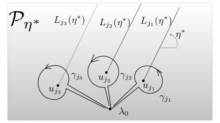
Figure 1: $\mathcal{P}_{\eta^{*}}$, branch-cuts and basic loops.

Remark 3.4.

From $c_{jk}=0$, the monodromy transformations (3.7) make sense also in case of coalescences in $\mathbb{D}=\mathbb{D}(u^{c})$. The base point $\lambda_{0}$ for the loops $\gamma_{j}$ is taken in $\bigcap_{u\in\mathbb{D}}\mathcal{P}_{\eta^{*}}(u)$ as in figure 1. In case of coalescence $u_{j}^{c}=u_{k}^{c}$, the two branch cuts $L_{j}(\eta)$ and $L_{k}(\eta)$ can overlap as $u$ varies in $\mathbb{D}(u^{c})$, but this causes no difficulties because $c_{jk}=0$, so that $\vec{\Psi}_{k}$ has trivial monodromy at $\lambda=u_{j}$.

It is important to notice that the matrix solution

$$\Psi(\lambda,u)=\Bigl{(}\vec{\Psi}_{1}(\lambda,u)~{}\Bigl{|}~{}\vec{\Psi}_{2}(\lambda,u)~{}\Bigr{|}~{}\vec{\Psi}_{3}(\lambda,u)\Bigr{)}$$ (3.8)

of (2.16) has constant monodromy, but it is not necessarily a fundamental matrix. It is fundamental if for example $V$ has no integer eigenvalues. If it happens that $V$ has some integer eigenvalues and $\Psi(\lambda,u)$ is fundamental, then necessarily there is at least one $\theta_{k}\in\mathbb{Z}$. This follows from [3] for the generic case and [39, 43] for the general case.

If $\mathbb{D}$ is as small has we have previously specified, an ordering relation is well defined in $\{1,2,3\}$:

• In case $\mathbb{D}=\mathbb{D}(u^{0})$, the ordering

  $$j\prec k\quad\Longleftrightarrow\quad\Re(e^{i\tau^{(0)}}(u_{j}-u_{k}))<0,\quad j\neq k.$$ (3.9)

  is well defined for all $u\in\mathbb{D}(u^{0})$. It coincides with the ordering defined by $\Re(e^{i\tau^{(0)}}(u_{j}^{0}-u_{k}^{0}))<0$. Equivalently, $j\prec k$ if and only if $L_{j}(\eta^{(0)})$ is to the right of $L_{k}(\eta^{(0)})$ in the $\lambda$-plane, where right or left refer to the orientation in direction $\eta^{(0)}$ towards infinity.

• In case of $\mathbb{D}=\mathbb{D}(u^{c})$, there is no ordering relation for $j,k$ such that $u_{j}^{c}=u_{k}^{c}$, while

  $$j\prec k\quad\Longleftrightarrow\quad\Re(e^{i\tau}(u_{j}-u_{k}))<0,\quad j\neq k\hbox{ and }u_{j}^{c}\neq u_{k}^{c}.$$ (3.10)

  If $\epsilon_{0}$ is as in Remark 3.1, then the partial ordering is well defined for all $u\in\mathbb{D}(u^{c})$. Notice that $j\prec k$ if and only if $L_{j}(\eta)$ is to the right of $L_{k}(\eta)$ in the $\lambda$-plane, or equivalently if $\mathcal{L}_{j}(\eta)$ is to the right of $\mathcal{L}_{k}(\eta)$ (see Remark 3.1).

Following [39, 43], the connection coefficients are related to the entries of the Stokes matrices of system (3.3) by

$$c_{jk}=\left\{\begin{array}[]{cc}\dfrac{e^{2\pi i\theta_{k}}}{\alpha_{k}}(\mathbb{S}_{1})_{jk},&j\prec k,\\ \\ -\dfrac{(\mathbb{S}_{2}^{-1})_{jk}}{e^{2\pi i(\theta_{j}-\theta_{k})}\alpha_{k}},&j\succ k.\end{array}\right.$$ (3.11)

We are ready to state the main result of the section.

Theorem 3.1.

Let $\mathbb{D}$ be $\mathbb{D}(u^{0})$, or $\mathbb{D}(u^{c})$. For every point $u^{\bullet}$ in $\mathbb{D}(u^{0})$, or in $\mathbb{D}(u^{c})\backslash\Delta_{\mathbb{C}^{3}}$, there is a neighborhood $\mathcal{U}$ of $u^{\bullet}$ in $\mathbb{D}$ and a fundamental matrix solution $\Phi_{\rm hol}(\lambda,u)$ of system (2.36), holomorphic of $(\lambda,u)\in\mathcal{P}_{\eta^{*}}(u)\hat{\times}~{}\mathcal{U}$ (here $\eta^{*}=\eta^{(0)}$ or $\eta$), whose monodromy invariants

$$p_{jk}:=\hbox{\rm tr}(\mathcal{M}_{j}(u)\mathcal{M}_{k}(u)),$$

are independent of $u$. Here, $\mathcal{M}_{j}(u)$ is the monodromy matrix at $\lambda=u_{j}$ of $\Phi_{\rm hol}(\lambda,u)$. They are expressed in terms of the Stokes matrices of system (3.3):

$$p_{jk}=\left\{\begin{array}[]{cc}2\cos\pi(\theta_{j}-\theta_{k})-e^{i\pi(\theta_{j}-\theta_{k})}(\mathbb{S}_{1})_{jk}(\mathbb{S}_{2}^{-1})_{kj},&j\prec k,\\ \\ 2\cos\pi(\theta_{j}-\theta_{k})-e^{i\pi(\theta_{k}-\theta_{j})}(\mathbb{S}_{1})_{kj}(\mathbb{S}_{2}^{-1})_{jk},,&j\succ k.\end{array}\right.$$ (3.12)

with ordering (3.9) or (3.10) according to the polydisc being either $\mathbb{D}(u^{0})$ or $\mathbb{D}(u^{c})$. In the latter case,

$$p_{jk}=2\cos\pi(\theta_{j}-\theta_{k})\quad\hbox{ for $j\neq k$ such that $u_{j}^{c}=u_{k}^{c}$}.$$

To appreciate the general validity of (3.12), notice that every fundamental solution $\Phi^{\prime}(\lambda,u)$ of system (2.36), defined at $u^{\bullet}$, is $\Phi^{\prime}(\lambda,u)=\Phi_{\rm hol}(\lambda,u^{\bullet})C^{\prime}(u)$, with $\det C^{\prime}(u)\neq 0$, so that its $\hbox{\rm tr}(\mathcal{M}^{\prime}_{j}\mathcal{M}^{\prime}_{k})$ coincide with $p_{jk}$ in (3.12).

Corollary 3.1.

The results of Theorem 3.1 hold for the monodromy invariants $p_{jk}$ of system (3.13) below, in terms of the Stokes matrices of system (2.10), where $\Omega$ is as in Theorem 2.1.

Proof.

It is elementary to check that the $2\times 2$ Fuchsian system (2.36) is equivalent to

$$\frac{d\widetilde{\Phi}}{d\widetilde{\lambda}}=\left(\frac{\widetilde{\mathcal{A}_{1}}(x)}{\widetilde{\lambda}}+\frac{\widetilde{\mathcal{A}_{2}}(x)}{\widetilde{\lambda}-x}+\frac{\widetilde{\mathcal{A}_{3}}(x)}{\widetilde{\lambda}-1}\right)\widetilde{\Phi},\quad\quad x=\frac{u_{2}-u_{1}}{u_{3}-u_{1}},$$ (3.13)

through the gauge transformation $\widetilde{\Phi}(\widetilde{\lambda},x)=(u_{3}-u_{1})^{\mathcal{A}_{\infty}}\Phi(\lambda,u)$ and change of variables $\widetilde{\lambda}=(\lambda-u_{1})/(u_{3}-u_{1})$. The Schlesinger system (2.43) (equivalent to PVI) expresses isomonodromy of (3.13). Now, we just take $u_{1}=0$, $u_{2}=x$, $u_{3}=1$ in the above discussion. ∎

3.1 Proof of Theorem 3.1

To the selected vector solutions $\vec{\Psi}_{1},\vec{\Psi}_{2},\vec{\Psi}_{3}$, we associate the solutions $\vec{X}_{k}(\lambda,u):=G^{-1}\vec{\Psi}_{k}$, $k=1,2,3$, of system (2.20). They have the same monodromy (3.7). Let

$$X(\lambda,u):=G^{-1}\Psi(\lambda,u)=\Bigl{(}\vec{X}_{1}(\lambda,u)~{}\Bigl{|}~{}\vec{X}_{2}(\lambda,u)~{}\Bigr{|}~{}\vec{X}_{3}(\lambda,u)\Bigr{)}=\begin{pmatrix}X_{1}^{1}&X_{2}^{1}&X_{3}^{1}\\ \vskip 6.0pt plus 2.0pt minus 2.0pt\cr X_{1}^{2}&X_{2}^{2}&X_{3}^{2}\\ \vskip 6.0pt plus 2.0pt minus 2.0pt\cr X_{1}^{3}&X_{2}^{3}&X_{3}^{3}\end{pmatrix}$$ (3.14)

be the matrix solution of system (2.20) corresponding to (3.8). From the entries in the first and third row we extract six matrix solutions (not necessarily fundamental) of the 2-dimensional system (2.26)

$$X^{[jk]}:=\begin{pmatrix}X_{j}^{1}&X_{k}^{1}\\ \vskip 6.0pt plus 2.0pt minus 2.0pt\cr X_{j}^{3}&X_{k}^{3}\end{pmatrix},\quad[jk]=[12],~{}[13],~{}[23],~{}[21],~{}[31],~{}[32].$$

Clearly, they reduce to $X^{[12]}$, $X^{[13]}$, $X^{[23]}$, because $X^{[kj]}=X^{[jk]}P$, $P:=\begin{pmatrix}0&1\\ 1&0\end{pmatrix}$. The column vectors of $X^{[jk]}$ will be written in bold symbol:

$$\boldsymbol{X}_{j}:=\begin{pmatrix}X_{j}^{1}\\ \vskip 6.0pt plus 2.0pt minus 2.0pt\cr X_{j}^{3}\end{pmatrix},\quad\quad\hbox{ so that }\quad X^{[jk]}(\lambda,u)=\Bigl{(}\boldsymbol{X}_{j}(\lambda,u)~{}\Bigr{|}~{}\boldsymbol{X}_{k}(\lambda,u)\Bigr{)}.$$

The monodromy properties (3.7) induce the following transformations:

$$\gamma_{1}:\quad\boldsymbol{X}_{1}\longmapsto e^{2\pi i\theta_{1}}\boldsymbol{X}_{1}, \boldsymbol{X}_{2}\longmapsto\boldsymbol{X}_{2}+\alpha_{1}c_{12}\boldsymbol{X}_{1}, \boldsymbol{X}_{3}\longmapsto\boldsymbol{X}_{3}+\alpha_{1}c_{13}\boldsymbol{X}_{1};$$ (3.15)

$$\gamma_{2}:\quad\boldsymbol{X}_{1}\longmapsto\boldsymbol{X}_{1}+\alpha_{2}c_{21}\boldsymbol{X}_{2}, \boldsymbol{X}_{2}\longmapsto e^{2\pi i\theta_{2}}\boldsymbol{X}_{2}, \boldsymbol{X}_{3}\longmapsto\boldsymbol{X}_{3}+\alpha_{2}c_{23}\boldsymbol{X}_{2};$$ (3.16)

$$\gamma_{3}:\quad\boldsymbol{X}_{1}\longmapsto\boldsymbol{X}_{1}+\alpha_{3}c_{31}\boldsymbol{X}_{3}, \boldsymbol{X}_{2}\longmapsto\boldsymbol{X}_{2}+\alpha_{3}c_{32}\boldsymbol{X}_{3}, \boldsymbol{X}_{3}\longmapsto e^{2\pi i\theta_{3}}\boldsymbol{X}_{3};$$ (3.17)

We distinguish two cases:

• there are two linearly independent $\boldsymbol{X}_{j}$, $\boldsymbol{X}_{k}$, $j\neq k$;

• all the $\boldsymbol{X}_{j}$ are linearly dependent.

We consider the linearly independent case first (it occurs for example if (3.8) is a fundamental matrix solution). Without loss of generality, we assume that $\boldsymbol{X}_{1}$ and $\boldsymbol{X}_{3}$ are linearly independent (otherwise, the analogous discussion holds for an independent pair $\boldsymbol{X}_{j},\boldsymbol{X}_{k}$). For the loops $\gamma_{1},\gamma_{2},\gamma_{3}$ we compute the monodromy matrices $\mathcal{M}_{1},\mathcal{M}_{2},\mathcal{M}_{3}$ of the following fundamental matrix solution of system (2.36)

$$\Phi_{\rm hol}(\lambda,u):=\Phi^{[13]}(\lambda,u)=\prod_{j=1}^{3}(\lambda-u_{j})^{-\theta_{j}/2}X^{[13]}(\lambda,u).$$ (3.18)

From (3.15) and (3.17) we receive

$$\mathcal{M}_{1}=\begin{pmatrix}e^{\pi i\theta_{1}}&e^{-\pi i\theta_{1}}\alpha_{1}c_{13}\\ \vskip 6.0pt plus 2.0pt minus 2.0pt\cr 0&e^{-\pi i\theta_{1}}\end{pmatrix},\quad\quad\mathcal{M}_{3}=\begin{pmatrix}e^{-\pi i\theta_{3}}&0\\ \vskip 6.0pt plus 2.0pt minus 2.0pt\cr e^{-\pi i\theta_{3}}\alpha_{3}c_{31}&e^{\pi i\theta_{3}}\end{pmatrix},$$

so that

$$p_{13}=e^{-i\pi(\theta_{1}+\theta_{3})}\alpha_{1}\alpha_{3}c_{13}c_{31}+2\cos(\pi(\theta_{1}-\theta_{3})).$$

Now, $\boldsymbol{X}_{2}=a\boldsymbol{X}_{1}+b\boldsymbol{X}_{3}$ for some $a,b\in\mathbb{C}$, so that for the loop $\gamma_{2}$ the transformation (3.16) yields

$$\mathcal{M}_{2}=e^{-i\pi\theta_{2}}\begin{pmatrix}1+\alpha_{2}c_{21}a&\alpha_{2}c_{23}a\\ \vskip 6.0pt plus 2.0pt minus 2.0pt\cr\alpha_{2}c_{21}b&1+\alpha_{2}c_{23}b\end{pmatrix}.$$

In order to find $a,b$, we use that trace and determinant, being invariant by conjugation, must be

$$\hbox{\rm Tr}\mathcal{M}_{2}=2\cos\pi\theta_{j},\quad\quad\det\mathcal{M}_{2}=1.$$ (3.19)

Using that $\alpha_{2}=e^{2i\pi\theta_{2}}-1$ for $\theta_{2}\not\in\mathbb{Z}$ and $\alpha_{2}=2\pi i$ for $\theta_{2}\in\mathbb{Z}$, both relations (3.19) turn out to be equivalent to

$$c_{21}a+c_{23}b=\left\{\begin{array}[]{cc}1,&\hbox{ if }\theta_{2}\not\in\mathbb{Z};\\ \vskip 6.0pt plus 2.0pt minus 2.0pt\cr 0,&\hbox{ if }\theta_{2}\in\mathbb{Z}.\end{array}\right.$$ (3.20)

In order to find other consitions on $a$ and $b$, we consider the transformation of $\boldsymbol{X}_{2}$ in (3.15) along the loop $\gamma_{1}$:

$$\boldsymbol{X}_{2} ~{}\longmapsto \boldsymbol{X}_{2}+\alpha_{1}c_{12}\boldsymbol{X}_{1}\equiv a\boldsymbol{X}_{1}+b\boldsymbol{X}_{3}+\alpha_{1}c_{12}\boldsymbol{X}_{1},$$

$$\boldsymbol{X}_{2}=a\boldsymbol{X}_{1}+b\boldsymbol{X}_{3} ~{}\longmapsto ae^{2i\pi\theta_{1}}\boldsymbol{X}_{1}+b(\boldsymbol{X}_{3}+\alpha_{1}c_{13}\boldsymbol{X}_{1}).$$

The above holds if and only if $a(e^{2i\pi\theta_{1}}-1)+\alpha_{1}(bc_{13}-c_{12})=0$. Thus

$$c_{13}b=\left\{\begin{array}[]{cc}c_{12}-a,&\hbox{ if }\theta_{2}\not\in\mathbb{Z};\\ \vskip 6.0pt plus 2.0pt minus 2.0pt\cr c_{12},&\hbox{ if }\theta_{2}\in\mathbb{Z}.\end{array}\right.$$ (3.21)

For the loop $\gamma_{3}$ in (3.17):

$$\boldsymbol{X}_{2} ~{}\longmapsto \boldsymbol{X}_{2}+\alpha_{3}c_{32}\boldsymbol{X}_{3}\equiv a\boldsymbol{X}_{1}+b\boldsymbol{X}_{3}+\alpha_{3}c_{32}\boldsymbol{X}_{3},$$

$$\boldsymbol{X}_{2}=a\boldsymbol{X}_{1}+b\boldsymbol{X}_{3} ~{}\longmapsto a(\boldsymbol{X}_{1}+\alpha_{3}c_{31}\boldsymbol{X}_{3})+be^{2\pi i\theta_{3}}\boldsymbol{X}_{3}.$$

The above is true if and only if $b(e^{2i\pi\theta_{3}}-1)+\alpha_{3}(ac_{31}-c_{32})=0$, namely

$$c_{31}a=\left\{\begin{array}[]{cc}c_{32}-b,&\hbox{ if }\theta_{2}\not\in\mathbb{Z};\\ \vskip 6.0pt plus 2.0pt minus 2.0pt\cr c_{32},&\hbox{ if }\theta_{2}\in\mathbb{Z}.\end{array}\right.$$ (3.22)

For the loop $\gamma_{2}$ in (3.16), the analogous procedure yields again (3.20).

We are ready to compute $\hbox{\rm Tr}(\mathcal{M}_{1}\mathcal{M}_{2})$. In case $\boldsymbol{X}_{1}$ and $\boldsymbol{X}_{2}$ are also independent (i.e. $b\neq 0$), since $\hbox{\rm Tr }(\mathcal{M}_{1}\mathcal{M}_{2})$ is invariant by conjugation, we can compute it using $\boldsymbol{X}_{1}$ and $\boldsymbol{X}_{2}$ as a basis, and this is done as above for the case $\boldsymbol{X}_{1},\boldsymbol{X}_{3}$, yielding

$$p_{12}=e^{-i\pi(\theta_{1}+\theta_{2})}\alpha_{1}\alpha_{2}c_{12}c_{21}+2\cos(\pi(\theta_{1}-\theta_{2})).$$

In case $\boldsymbol{X}_{1}$ and $\boldsymbol{X}_{2}$ are not independent, then $b=0$ and

$$\mathcal{M}_{2}=\begin{pmatrix}e^{-i\pi\theta_{2}}(1+\alpha_{2}c_{21}a)&e^{-i\pi\theta_{2}}\alpha_{2}c_{23}a\\ \vskip 6.0pt plus 2.0pt minus 2.0pt\cr 0&e^{-i\pi\theta_{2}}\end{pmatrix}.$$

From (3.20), (3.21), (3.22) we receive

$$c_{21}a=\left\{\begin{array}[]{cc}1,&\hbox{ if }\theta_{2}\not\in\mathbb{Z},\\ \vskip 6.0pt plus 2.0pt minus 2.0pt\cr 0,&\hbox{ if }\theta_{2}\in\mathbb{Z},\end{array}\right.\quad 0=\left\{\begin{array}[]{cc}c_{12}-a,&\hbox{ if }\theta_{2}\not\in\mathbb{Z},\\ \vskip 6.0pt plus 2.0pt minus 2.0pt\cr c_{12},&\hbox{ if }\theta_{2}\in\mathbb{Z},\end{array}\right.\quad\quad\quad c_{31}a=c_{32}.$$

For $\theta_{2}\not\in\mathbb{Z}$:

$$a=c_{12}=\frac{1}{c_{21}},\quad\quad\hbox{ and }\quad c_{12}c_{21}=1,\quad c_{32}=c_{31}c_{12}.$$

Using $\alpha_{2}=\exp\{2\pi i\theta_{2}\}-1$, we receive

$$\mathcal{M}_{2}=\begin{pmatrix}e^{i\pi\theta_{2}}&2i\sin(\pi\theta_{2})c_{12}c_{23}\\ \vskip 6.0pt plus 2.0pt minus 2.0pt\cr 0&e^{-i\pi\theta_{2}}\end{pmatrix},$$

so that

$$p_{12}=2\cos(\pi(\theta_{1}+\theta_{2}))\underset{c_{12}c_{21}=1}{\equiv}2c_{12}c_{21}(\cos\pi(\theta_{1}+\theta_{2})-\cos\pi(\theta_{1}-\theta_{2}))+2\cos\pi(\theta_{1}-\theta_{2})$$

For $\theta_{2}\in\mathbb{Z}$:

$$ac_{21}=0,\quad c_{12}=0.$$

Recalling that $\alpha_{2}=2\pi i$, we receive

$$\mathcal{M}_{2}=(-1)^{\theta_{2}}\begin{pmatrix}1&2\pi ic_{23}a\\ \vskip 6.0pt plus 2.0pt minus 2.0pt\cr 0&1\end{pmatrix},\quad c_{31}a=c_{32}.$$

Therefore

$$p_{12}=(-1)^{\theta_{2}}2\cos(\pi\theta_{1})\underset{c_{12}=0}{\equiv}2c_{12}c_{21}(\cos\pi(\theta_{1}+\theta_{2})-\cos\pi(\theta_{1}-\theta_{2}))+2\cos\pi(\theta_{1}-\theta_{2}).$$

The computation of $p_{23}=\hbox{\rm Tr}(\mathcal{M}_{2}\mathcal{M}_{3})$ can be done in an analogous way. In conclusion, all the possibilities considered are summarized in the formula

$$p_{jk}=e^{-i\pi(\theta_{j}+\theta_{k})}\alpha_{j}\alpha_{k}c_{jk}c_{kj}+2\cos(\pi(\theta_{j}-\theta_{k})).$$ (3.23)

Finally, we substitute (3.11) and receive (3.12) in full generality.

$\bullet$ We consider the linearly-dependent case. We do a gauge transformation ${}_{\gamma}Y:=z^{-\gamma}Y$, $\gamma\in\mathbb{C}$, which transforms (2.15) into

$$d({}_{\gamma}Y)=\omega(z,u;\gamma)~{}{}_{\gamma}Y,\quad\quad\omega(z,u;\gamma)=\left(U+\frac{\widetilde{V}-\gamma I}{z}\right)dz+\sum_{k=1}^{3}(zE_{k}+V_{k})du_{k},$$

where $\widetilde{V}:=V-I$. This changes $\theta_{k}\mapsto\theta_{k}+\gamma$, while $\theta_{\infty}$ is unchanged, and (2.38) changes to $\mu_{1}[\gamma]=(\theta_{\infty}-\theta_{1}-\theta_{2}-\theta_{3}-3\gamma)/2$, $\mu_{3}[\gamma]=(-\theta_{\infty}-\theta_{1}-\theta_{2}-\theta_{3}-3\gamma)/2$.

There exists $\gamma_{0}>0$ sufficiently small such that $V-\gamma$ and $\widetilde{V}-\gamma$ have non-integer eigenvalues and non-integer diagonal entries for $0<|\gamma|<\gamma_{0}$. Hence, the analogous of the matrix (3.8), here called ${}_{\gamma}\Psi(\lambda,u)=\bigl{(}{}_{\gamma}\vec{\Psi}_{1}(\lambda,u)~{}\bigl{|}~{}{}_{\gamma}\vec{\Psi}_{2}(\lambda,u)~{}\bigr{|}~{}{}_{\gamma}\vec{\Psi}_{3}(\lambda,u)\bigr{)}$, is fundamental. The connection coefficients in (3.7), depending on $\gamma$, will be called $c_{jk}[\gamma]$, with

$$\alpha_{k}[\gamma]=e^{2\pi i(\theta_{k}+\gamma)}-1.$$

Consequently, there are two independent column vectors in the triple ${}_{\gamma}\boldsymbol{X}_{1}(\lambda,u),{}_{\gamma}\boldsymbol{X}_{2}(\lambda,u),{}_{\gamma}\boldsymbol{X}_{3}(\lambda,u)$. The discussion of the independent case can be repeated, with the $c_{jk}[\gamma]$ and $\alpha_{k}[\gamma]$ in the transformations (3.15)-(3.17). We can assume that ${}_{\gamma}\boldsymbol{X}_{1}$ and ${}_{\gamma}\boldsymbol{X}_{3}$ are independent, otherwise the discussion is analogous for another independent pair ${}_{\gamma}\boldsymbol{X}_{j}$, ${}_{\gamma}\boldsymbol{X}_{k}$. After the gauge

$${}_{\gamma}{\Phi}=\prod_{j=1}^{3}(\lambda-u_{j})^{-(\theta_{j}+\gamma)/2}~{}{}_{\gamma}\boldsymbol{X},$$

we obtain the analogous of system (2.36):

$$\frac{d({}_{\gamma}\Phi)}{d\lambda}=\sum_{k=1}^{3}\frac{\mathcal{A}_{k}[\gamma]}{\lambda-u_{k}}~{}{}_{\gamma}\Phi,\quad\quad\mathcal{A}_{k}:=A_{k}[\gamma]-\frac{\theta_{k}+\gamma}{2}.$$ (3.24)

Let

$${}_{\gamma}\Phi^{[1,3]}(\lambda,u)=\prod_{j=1}^{3}(\lambda-u_{j})^{-\theta_{j}/2}\Bigl{(}{}_{\gamma}\boldsymbol{X}_{1}(\lambda,u)~{}\Bigr{|}~{}{}_{\gamma}\boldsymbol{X}_{3}(\lambda,u)\Bigr{)}$$

be the analogous of (3.18), and let $\mathcal{M}_{j}[\gamma]$ be its monodromy matrix at $u_{j}$. The same procedure which has proved (3.23) yields

$$p_{jk}[\gamma] :=\hbox{\rm Tr}(\mathcal{M}_{j}[\gamma]\mathcal{M}_{k}[\gamma])$$ (3.25)

$$=e^{-i\pi(\theta_{j}+\theta_{k}+2\gamma)}\alpha_{j}[\gamma]\alpha_{k}[\gamma]c_{jk}[\gamma]c_{kj}[\gamma]+2\cos(\pi(\theta_{j}-\theta_{k})),\quad j\neq k.$$

In general the $\gamma$-dependent objects $c_{jk}[\gamma]$, ${}_{\gamma}\Psi$, ${}_{\gamma}\boldsymbol{X}_{k}$ and ${}_{\gamma}\Phi^{[1,3]}$ diverge for $\gamma\to 0$. Therefore, the monodromy matrices $\mathcal{M}_{1}[\gamma]$, $\mathcal{M}_{2}[\gamma]$, $\mathcal{M}_{3}[\gamma]$ generate the monodromy group for $0<|\gamma|<\gamma_{0}$, but may be not defined at $\gamma=0$. To overcome the problem, we use a relation proved in full generality in [39], and in [3] in a generic case. In case $\mathbb{D}=\mathbb{D}(u^{0})$, the relation says that at any $u\in\mathbb{D}(u^{0})$

$$\alpha_{k}c_{jk}=\begin{cases}\begin{aligned} e^{-2\pi i\gamma}\alpha_{k}[\gamma]~{}c_{jk}[\gamma],&&\hbox{ if }k\succ j,\\[4.30554pt] \alpha_{k}[\gamma]~{}c_{jk}[\gamma],&&\hbox{ if }k\prec j,\end{aligned}\end{cases}\quad\quad\hbox{for real }0<\gamma<\gamma_{0}.$$ (3.26)

The ordering $k\prec j$ is (3.9), well defined and the same at any $u\in\mathbb{D}(u^{0})$. In case $\mathbb{D}=\mathbb{D}(u^{c})$, the same relation holds at any $u\in\mathbb{D}(u^{c})\backslash\Delta_{\mathbb{C}^{3}}$ for $j\neq k$ such that $u_{j}^{c}\neq u_{k}^{c}$, the ordering relation (3.10) being well defined for every $u\in\mathbb{D}(u^{c})\backslash\Delta_{\mathbb{C}^{3}}$. For $j\neq k$ such that $u_{j}^{c}=u_{k}^{c}$ the ordering relation is not defined, but $c_{jk}=c_{jk}[\gamma]=0$, so that we can state that (3.26) still holds. Using (3.26), (3.25) becomes

$$p_{jk}[\gamma]=e^{i\pi\gamma}~{}e^{-i\pi(\theta_{j}+\theta_{k})}\alpha_{j}\alpha_{k}c_{jk}c_{kj}+2\cos(\pi(\theta_{j}-\theta_{k})),\quad\quad 0<\gamma<\gamma_{0}\hbox{ real},$$ (3.27)

for both $u\in\mathbb{D}(u^{0})$ and $u\in\mathbb{D}(u^{c})\backslash\Delta_{\mathbb{C}^{3}}$ (in the latter case, (3.27) is true also for $j\neq k$ such that $u_{j}^{c}=u_{k}^{c}$, because it just reduces to the identity $2\cos(\pi(\theta_{j}-\theta_{k}))=2\cos(\pi(\theta_{j}-\theta_{k}))$). Since both the $c_{jk}$ and $c_{jk}[\gamma]$ are constant, (3.27) extends analytically at $\Delta_{\mathbb{C}^{3}}$.

The r.h.s. of (3.27) depends holomorphically on $\gamma\in\mathbb{C}$, while the l.h.s. $p_{jk}[\gamma]$ has been computed from ${}_{\gamma}\Phi^{[13]}$, which is not in general defined for $\gamma=0$. We show that $p_{jk}[\gamma]$ can also be obtained from a fundamental matrix solution of (3.24) which is holomorphic of $\gamma$ in a neighbourhood of $\gamma=0$. To do that, we need to recall from [14] that if $\mathbb{D}=\mathbb{D}(u^{c})$, the choice of an admissible direction $\tau$ determines a cell decomposition of $\mathbb{D}(u^{c})$ into topological cells, called $\tau$-cells. They are the connected components of $\mathbb{D}(u^{c})\backslash(\Delta_{\mathbb{C}^{3}}\cup X(\tau))$, where $X(\tau)$ is the locus of points $u=(u_{1},u_{2},u_{3})\in\mathbb{D}(u^{c})$ such that $\Re(e^{i\tau}(u_{j}-u_{k}))=0$.

For $\mathbb{D}=\mathbb{D}(u^{0})$, let $u^{\bullet}\in\mathbb{D}(u^{0})$. For $\mathbb{D}=\mathbb{D}(u^{c})$, let $u^{\bullet}$ belong to a $\tau$-cell of $\mathbb{D}(u^{c})$. Then, there is a sufficiently small neighbourhood $\mathcal{U}$ of $u^{\bullet}$ such that, as $u$ varies in $\mathcal{U}$, then $u_{k}$ represented in the $\lambda$-plane remains inside a closed disc $D_{k}$ centered at $u^{\bullet}_{k}$, with $D_{j}\cap D_{k}=\emptyset$ for $1\leq j\neq k\leq 3$. Consider the simply connected domain

$$\mathcal{B}_{u^{\bullet}}:=\mathcal{P}_{\eta^{*}}(u^{\bullet})\backslash(D_{1}\cup D_{2}\cup D_{3}).$$

Since system (3.24) holomorphically depends on the parameters $(u,\gamma)\in\mathcal{U}\times\{\gamma\in\mathbb{C}\hbox{ s.t. }|\gamma|<\gamma_{0}\}$, according to a general result (see for example [63]) it has a fundamental matrix solution

$$\Phi_{\rm hol}^{(u^{\bullet})}(\lambda,u,\gamma)$$

holomorphic of $(\lambda,u,\gamma)\in\mathcal{B}_{u^{\bullet}}\times\mathcal{U}\times\{\gamma\in\mathbb{C}\hbox{ s.t. }|\gamma|<\gamma_{0}\}$. If $\mathcal{U}$ is sufficiently small, it holomorphically extends to $\bigl{(}\mathcal{P}_{\eta^{*}}(u)\widehat{\times}~{}\mathcal{U}\bigr{)}\times\{\gamma\in\mathbb{C}\hbox{ s.t. }|\gamma|<\gamma_{0}\}$. For some invertible connection matrix $C(u,\gamma)$ we have

$$\Phi_{\rm hol}^{(u^{\bullet})}(\lambda,u,\gamma)={}_{\gamma}\Phi^{[13]}(\lambda,u)\cdot C(u,\gamma),\quad 0<|\gamma|<\gamma_{0}.$$

Now, $C(u,\gamma)$ is holomorphic of $u\in\mathcal{U}$, for any $0<|\gamma|<\gamma_{0}$, but may diverge as $\gamma\to 0$. On the other hand, the monodromy matrix $\mathcal{M}_{k}^{\rm hol}(u,\gamma)$ of $\Phi_{\rm hol}^{(u^{\bullet})}(\lambda,u,\gamma)$ at $\lambda=u_{k}$, is holomorphic of $(u,\gamma)\in\mathcal{U}\times\{\gamma\in\mathbb{C}\hbox{ s.t. }|\gamma|<\gamma_{0}\}$, including $\gamma=0$. Moreover,

$$\mathcal{M}_{k}[\gamma]=C(u,\gamma)\cdot\mathcal{M}_{k}^{\rm hol}(u,\gamma)\cdot C(u,\gamma)^{-1}.$$

Since $\hbox{\rm Tr}(\mathcal{M}_{j}^{\rm hol}(u,\gamma)\mathcal{M}_{k}^{\rm hol}(u,\gamma))=\hbox{\rm Tr}(\mathcal{M}_{j}[\gamma]\mathcal{M}_{k}[\gamma])\equiv p_{jk}[\gamma]$, we see from (3.27) that

$$\hbox{\rm Tr}(\mathcal{M}_{j}^{\rm hol}(u,\gamma)\mathcal{M}_{k}^{\rm hol}(u,\gamma))=e^{i\pi\gamma}~{}e^{-i\pi(\theta_{j}+\theta_{k})}\alpha_{j}\alpha_{k}c_{jk}c_{kj}+2\cos(\pi(\theta_{j}-\theta_{k})),\quad\quad 0<\gamma<\gamma_{0}.$$

Now, both $\hbox{\rm Tr}(\mathcal{M}_{j}^{\rm hol}(u,\gamma)\mathcal{M}_{k}^{\rm hol}(u,\gamma))$ and $p_{jk}[\gamma]$ are continuous of $\gamma$ in a neighbourhood of $\gamma=0$. Therefore we are allowed to take the limit $\gamma\to 0_{+}$ and obtain

$$p_{jk}:=\hbox{\rm Tr}(\mathcal{M}_{j}^{\rm hol}(u,0)\mathcal{M}_{k}^{\rm hol}(u,0))=~{}e^{-i\pi(\theta_{j}+\theta_{k})}\alpha_{j}\alpha_{k}c_{jk}c_{kj}+2\cos(\pi(\theta_{j}-\theta_{k})).$$ (3.28)

In case $\mathbb{D}=\mathbb{D}(u^{c})$, we can repeat the above discussion also for $u^{\bullet}$ on the boundary of one $\tau$-cell (provided that $u^{\bullet}\not\in\Delta_{\mathbb{C}^{3}}$), because $\tau=3\pi/2-\eta$ can be slightly changed without affecting the properties of fundamental solutions.

Now, also at $\gamma=0$ the matrix

$$\Phi_{\rm hol}^{(u^{\bullet})}(\lambda,u,0)$$

is a fundamental solution of system (2.36). Therefore, we have proved that for every $u^{\bullet}\in\mathbb{D}(u^{0})$ or $u^{\bullet}\in\mathbb{D}(u^{c})\backslash\Delta_{\mathbb{C}^{3}}$, we can find a fundamental solution $\Phi_{\rm hol}^{(u^{\bullet})}(\lambda,u,0)$ of system (2.36), holomorphically depending on $(\lambda,u)\in\mathcal{P}_{\eta^{*}}(u)\widehat{\times}~{}\mathcal{U}$, with $\mathcal{U}$ small enough, such that its monodromy invariants are the $p_{jk}$ in (3.28). Thus, we conclude that the formulae (3.12) always hold. $\Box$

Notice that in the linearly dependent case, $\Phi_{\rm hol}(\lambda,u)$ in the statement of the theorem is precisely $\Phi_{\rm hol}^{(u^{\bullet})}(\lambda,u,0)$ above, while in the linearly independent case it is a fundamental matrix like (3.18).

4 Classification of analytic solutions of PVI satisfying theorem 1.1 of [14]. Reduction to special functions

We study system (2.10) whose $\Omega(x)$ is associated, through Theorem 2.1, with PVI transcendents that admit a Taylor expansion near a critical point. By the symmetries of PVI, it suffices to only consider $x=0$. Our first goal is to classify those transcendents with behaviour $y(x)=\sum_{n=0}^{\infty}b_{n}x^{n}$ at $x=0$ such that theorem 1.1 of [14] applies, namely such that $\Omega(x)$ is holomorphic at $x=0$ and

$$\lim_{x\to 0}\Omega_{12}(x)=\lim_{x\to 0}\Omega_{21}(x)=0\quad\hbox{ holomorphically}.$$ (4.1)

As already explained in the Introduction, since Jimbo’s work [53], the strategy to solve the non-linear connection problem for a transcendent $y(x)$ has been to parameterize the integration constants determining the critical behaviour at $x=0,1$ or $\infty$ in terms of $\theta_{1}$, $\theta_{2}$, $\theta_{3}$, $\theta_{\infty}$ and the traces $p_{jk}$ of the $2\times 2$ Fuchsian system (3.13) associated with $y(x)$. Theorem 3.1 and Corollary 3.1 allow us to obtain the $p_{jk}$’s in terms of the Stokes matrices of (2.10) (with $\Omega$ of Theorem 2.1). According to theorem 1.1 of [14], when (4.1) holds all the monodromy data of system (2.10) on a polydisc can be computed from the system at the fixed coalescence point $x=0$:

$$\frac{dY}{dz}=\left(U_{0}+\frac{\Omega_{0}}{z}\right)Y,\quad\quad U_{0}:=\mbox{diag}(0,0,1),\quad\Omega_{0}:=\Omega(0).$$ (4.2)

The latter is simpler than (2.10), because $\Omega_{12}(0)=\Omega_{21}(0)=0$.

The second goal of this section is to show that for the transcendents with Taylor series at $x=0$ such that (4.1) holds, system (4.2) is reduced to the confluent hypergeometric equation (equivalently, a Whittaker equation, and for special cases a Bessel equation) or to the generalized hypergeometric equation of type $(q,p)=(2,2)$. This implies that the Stokes matrices can be computed using classical special functions. Some selected examples of this computation will be the object of Section 5.

The first column of the table below reproduces the table of [37] for transcendents with Taylor series at $x=0$, and corrects minor misprints there. The parameters $\theta_{1},\theta_{2},\theta_{3},\theta_{\infty}$ and the free parameter (the integration constant) $y_{0}$ or $y_{0}^{(|N|)}$ in $y(x)$, if any, must satisfy the conditions in the second column. In the third column, we give our classification according to the fulfilment of the vanishing conditions (4.1) and indicate the classical special functions in terms of which (4.2) can be solved. In the subsequent sub-sections we present the details of this classification. For the classical special functions, we refer to Appendix A. For $N\in\mathbb{Z}\backslash\{0\}$ we also define

$$\mathcal{N}_{N}:=\begin{cases}\{0,2,4,\ldots,|N|-1\}\cup\{-2,-4,\ldots,-(|N|-1)\},&\mbox{if }N\mbox{ is odd}\\ \{1,3,\ldots,|N|-1\}\cup\{-1,-3,\ldots,-(|N|-1)\},&\mbox{if }N\mbox{ is even}.\end{cases}$$ (4.3)

Taylor series	Conditions on parameters	Classical special functions
$\displaystyle{y(x)=y_{0}+\sum_{n\geq 1}b_{n}(y_{0})~{}x^{n}}$	$\displaystyle{y_{0}=\frac{\theta_{\infty}-1+\theta_{3}}{\theta_{\infty}-1}}$ $\theta_{\infty}+\theta_{3}\notin\mathbb{Z}$ $\theta_{\infty}\neq 1$ or $\displaystyle{y_{0}=\frac{\theta_{\infty}-1-\theta_{3}}{\theta_{\infty}}}$ $\theta_{\infty}-\theta_{3}\notin\mathbb{Z}$ $\theta_{\infty}\neq 1$	The vanishing condition (4.1) does not hold
$y(x)=y_{0}+\displaystyle\sum_{n\geq 1}b_{n}(y_{0})~{}x^{n}$	$\theta_{3}=0,\,\theta_{\infty}=1$ $y_{0}$ free parameter
$\displaystyle{y(x)=\sum_{n=0}^{|N|-1}b_{n}x^{n}+\frac{y_{0}^{(|N|)}}{(|N|)!}x^{|N|}}$ $\quad\quad\displaystyle{+\sum_{n\geq|N|+1}b_{n}(y_{0}^{(|N|)})~{}x^{n}}$ (T1)	$\displaystyle{b_{0}=\frac{N}{\theta_{\infty}-1}},~{}\theta_{\infty}\neq 1.$ $y_{0}^{(|N|)}\mbox{ free parameter}.$ $\theta_{\infty}-1+\theta_{3}=N\in\mathbb{Z}\setminus\{0\}$ or $\theta_{\infty}-1-\theta_{3}=N\in\mathbb{Z}\setminus\{0\}$, and $\theta_{1}-\theta_{2}\in\mathcal{N}_{N}$	Confluent hypergeometric
	$\displaystyle{b_{0}=\frac{N}{\theta_{\infty}-1}},~{}\theta_{\infty}\neq 1.$ $y_{0}^{(|N|)}\mbox{ free parameter.}$ $\theta_{\infty}-1+\theta_{3}=N\in\mathbb{Z}\setminus\{0\}$ or $\theta_{\infty}-1-\theta_{3}=N\in\mathbb{Z}\setminus\{0\},$ and either $\theta_{\infty}-1\in\begin{cases}\{-1,\ldots,-|N|+1\}\\ \{1,\ldots,|N|-1\}\end{cases}$ or $\theta_{1}+\theta_{2}\in\mathcal{N}_{N}$	The vanishing condition (4.1) does not hold
$\displaystyle{y(x)=y_{0}^{\prime}x+\sum_{n\geq 2}b_{n}(y_{0}^{\prime})~{}x^{n}}$ (T2)	$\displaystyle{y_{0}^{\prime}=\frac{\theta_{1}}{\theta_{1}-\theta_{2}},\quad\theta_{1}-\theta_{2}\not\in\mathbb{Z}}$	$(2,2)$ - Generalized hypergeometric
	$\displaystyle{y_{0}^{\prime}=\frac{\theta_{1}}{\theta_{1}+\theta_{2}}},\quad\theta_{1}+\theta_{2}\not\in\mathbb{Z}$	For $\theta_{2}=0$ case above Otherwise: the vanishing condition (4.1) does not hold
$\displaystyle{y(x)=y_{0}^{\prime}x+\sum_{n\geq 2}b_{n}(y_{0}^{\prime})~{}x^{n}}$ (T3)	$\theta_{1}=\theta_{2}=0$ $y_{0}^{\prime}$ free parameter	Confluent hypergeometric
$\displaystyle{y(x)=\sum_{n=1}^{|N|}b_{n}x^{n}}$ $\quad\quad\displaystyle{+\frac{y_{0}^{(|N|+1)}}{(|N|+1)!}x^{|N|+1}}$ $\quad\quad\displaystyle{+\sum_{n\geq|N|+2}b_{n}(y_{0}^{(|N|+1)})~{}x^{n}}$ (T4)	$\theta_{1}-\theta_{2}=N\in\mathbb{Z}\setminus\{0\}$ $\theta_{1}\in\begin{cases}\{-1,-2,\ldots,-|N|+1\}\\ \{1,2,\ldots,|N|-1\}\end{cases}$ $y_{0}^{(|N|+1)}$ free parameter	$(2,2)$ - Generalized hypergeometric
	$\theta_{1}-\theta_{2}=N\in\mathbb{Z}\setminus\{0\}$ or $\theta_{1}+\theta_{2}=N\in\mathbb{Z}\setminus\{0\}$ and $\theta_{1}=0,N,$ $y_{0}^{(|N|+1)}$ free parameter	Confluent hypergeometric
	$\theta_{1}-\theta_{2}=N\in\mathbb{Z}\setminus\{0\}$ $\{(\theta_{3}+\theta_{\infty}-1),$ $(-\theta_{3}+\theta_{\infty}-1)\}\cap\mathcal{N}_{N}\neq\emptyset$ $y_{0}^{(|N|+1)}$ free parameter	$(2,2)$ - Generalized hypergeometric
	$\theta_{1}+\theta_{2}=N\in\mathbb{Z}\setminus\{0\}$ $\theta_{1}\in\begin{cases}\{-1,-2,\ldots,-|N|+1\}\\ \{1,2,\ldots,|N|-1\}\end{cases}$ or $\{(\theta_{3}+\theta_{\infty}-1),$ $(-\theta_{3}+\theta_{\infty}-1)\}\cap\mathcal{N}_{N}\neq\emptyset$ $y^{(|N|+1)}_{0}$ free parameter	The vanishing condition (4.1) does not hold

Remark 4.1.

In the table of [37] there is a missprint. Corresponding to the branches (45), the correct condition is $\sqrt{-2\beta}\in\{-1,-2,N+1\}$ for $N<0$, and $\sqrt{-2\beta}\in\{1,2,N-1\}$ for $N>0$. In (61), the correct condition is $\sqrt{2\alpha}\in\{-1,-2,N+1\}$ for $N<0$, and $\sqrt{2\alpha}\in\{1,2,N-1\}$ for $N>0$.

4.1 Transcendents with Taylor expansion $y(x)=y_{0}+O(x)$

We study the behaviour of $\Omega(x)$ as given in Theorem 2.1 when $y(x)=y_{0}+O(x)$, where $O(x)=\sum_{n\geq 1}b_{n}x^{n}$ is a Taylor series in a neighborhood of $x=0$. The functions $k_{1}$, $k_{2}$ can be written as

$$k_{1}(x)=k_{1}^{0}(1+O(x))\frac{\sqrt{y}(x-1)^{(1+\theta_{2})/2}}{\sqrt{y-1}x^{(1+\theta_{2})/2}}x^{(\theta_{1}+\theta_{3}y_{0}/(y_{0}-1))/2},$$

$$k_{2}(x)=k_{2}^{0}(1+O(x))\frac{\sqrt{y-x}(x-1)^{\theta_{2}-\theta_{3}}}{\sqrt{y-1}x^{(1+\theta_{1})/2}}x^{(\theta_{2}+\theta_{3}y_{0}/(y_{0}-1))/2}, k_{1}^{0},k_{2}^{0}\in\mathbb{C}\backslash\{0\}.$$

Hence, the off diagonal elemets of the matrix $\Omega(x)$ have the structure

$$\Omega_{12}(x) =\omega_{12}(x)x^{\theta_{1}-\theta_{2}}, \Omega_{13}(x) =\omega_{13}(x)x^{(\theta_{1}+\theta_{3}y_{0}/(y_{0}-1)-\theta_{2}-1)/2},$$

$$\Omega_{21}(x) =\omega_{21}(x)x^{\theta_{2}-\theta_{1}}, \Omega_{23}(x) =\omega_{23}(x)x^{(\theta_{2}+\theta_{3}y_{0}/(y_{0}-1)-\theta_{1}-1)/2},$$

$$\Omega_{31}(x) =\omega_{31}(x)x^{-(\theta_{1}+\theta_{3}y_{0}/(y_{0}-1)-\theta_{2}-1)/2-1}, \Omega_{32}(x) =\omega_{32}(x)x^{-(\theta_{2}+\theta_{3}y_{0}/(y_{0}-1)-\theta_{1}-1)/2-1},$$

where $\omega_{ij}(x)$ are holomorphic functions at $x=0$, explicitly computed from the formulae of Theorem 2.1.

There are three classes of solutions $y(x)=y_{0}+O(x)$, obtained in [33] and classified in the tables of [37]. The generic one is

$$y(x)=y_{0}(\theta_{\infty},\theta_{3})+\sum_{n=1}^{\infty}b_{n}(\vec{\theta})x^{n},\quad\quad\theta_{\infty}\neq 1,\quad\vec{\theta}=(\theta_{1},\theta_{2},\theta_{3},\theta_{\infty}),$$ (4.4)

with two possibilities

$$y_{0}=\frac{\theta_{\infty}-1+\theta_{3}}{\theta_{\infty}-1},\quad\theta_{\infty}+\theta_{3}\notin\mathbb{Z};\quad\quad\hbox{ or }\quad\quad y_{0}=\frac{\theta_{\infty}-1-\theta_{3}}{\theta_{\infty}-1},\quad\theta_{\infty}-\theta_{3}\notin\mathbb{Z}.$$

The coefficients $\{b_{n}\}_{n\geq 1}$ are uniquely determined when $y_{0}$ is decided between the two possibilities. The other two classes consist of the following one-parameter families of solutions: the family

$$y(x)=y_{0}+\frac{(1-y_{0})(1+\theta_{1}^{2}-\theta_{2}^{2})}{2}x+\sum_{n=2}^{\infty}b_{n}(y_{0},\theta_{1},\theta_{2})x^{n},\quad\theta_{3}=0,\quad\theta_{\infty}=1,$$ (4.5)

where $y_{0}$ is a free parameter, and the family

$$y(x)=\sum_{n=0}^{|N|-1}b_{n}(\vec{\theta})x^{n}+\frac{y_{0}^{(|N|)}}{(|N|)!}x^{|N|}+\sum_{n=|N|+1}^{\infty}b_{n}(y_{0}^{(|N|)},\vec{\theta})x^{n},$$ (4.6)

where $y_{0}^{(|N|)}$ is a free parameter, $N\in\mathbb{Z}\setminus\{0\}$, the leading order coefficient is $b_{0}=N/(\theta_{\infty}-1)$, $\theta_{\infty}\neq 1$, and the conditions

$$\theta_{\infty}-1+\theta_{3}=N\quad\hbox{ or }\quad\theta_{\infty}-1-\theta_{3}=N$$

hold, with either

$$\theta_{\infty}-1\in\begin{cases}\{-1,-2,\ldots,N+1\}&\mbox{if }N<0\\ \{1,2,\ldots,N-1\}&\mbox{if }N>0\end{cases}$$ (4.7)

or (here, $\mathcal{N}_{N}$ is (4.3))

$$\{(\theta_{1}+\theta_{2}),\,(\theta_{1}-\theta_{2})\}\cap\mathcal{N}_{N}\neq\emptyset.$$ (4.8)

4.1.1 Generic case (4.4)

We show that the vanishing condition (4.1) does not hold. Let us consider the solution (4.4) with

$$y_{0}=\frac{\theta_{\infty}-1-\theta_{3}}{\theta_{\infty}-1},\quad\theta_{\infty}-\theta_{3}\notin\mathbb{Z},\quad\theta_{\infty}\neq 1.$$

If $\operatorname{Re}(\theta_{1}-\theta_{2})=0$, then the condition (4.1) is equivalent to $\theta_{1}=\theta_{2}$ and $\theta_{3}=\theta_{\infty}$, so that $\theta_{\infty}-\theta_{3}=0$, which is a contradiction.

If $\operatorname{Re}(\theta_{1}-\theta_{2})>0$, then $\lim_{x\to 0}\Omega_{12}(x)=0$ and for the requirement $\lim_{x\to 0}\Omega_{21}(x)=0$ to be fulfilled it is necessary that $\omega_{21}(0)=0$, that is (from the explicit formulae)

$$\theta_{1}=\theta_{2}+\theta_{3}-\theta_{\infty},$$ (4.9)

implying $\operatorname{Re}(\theta_{3}-\theta_{\infty})>0$. The functions $\Omega_{31}(x)$ and $\Omega_{21}(x)$ are then

$$\Omega_{31}(x)=\left(\frac{\omega^{\prime\prime}_{31}(0)}{2}x^{2}+O(x^{3})\right)x^{-(\theta_{3}-\theta_{\infty}+1)}=x\left(\frac{\omega^{\prime\prime}_{31}(0)}{2}+O(x)\right)x^{-(\theta_{3}-\theta_{\infty})},$$

$$\Omega_{21}(x)=\left(\frac{\omega^{\prime\prime}_{21}(0)}{2}x^{2}+O(x^{3})\right)x^{\theta_{2}-\theta_{1}}=x^{2}\left(\frac{\omega^{\prime\prime}_{21}(0)}{2}+O(x)\right)x^{-(\theta_{3}-\theta_{\infty})}.$$

The entry (3,1)

$$\frac{d\Omega_{31}}{dx}=\frac{\Omega_{32}\Omega_{21}}{x(x-1)},$$ (4.10)

of the isomonodromic deformation equation (2.8) gives

$$\frac{\omega^{\prime\prime}_{31}(0)}{2}(\theta_{\infty}-\theta_{3}+1)+O(x)=0,\quad\hbox{ which implies }\theta_{\infty}=\theta_{3}-1,$$

giving a contradiction.

If $\operatorname{Re}(\theta_{1}-\theta_{2})<0$, than $\lim_{x\to 0}\Omega_{21}(x)=0$ and a necessary condition for $\Omega_{12}(x)$ to vanish as $x\to 0$ is $\omega_{12}(0)=0$, that is (from the explicit formulae)

$$\theta_{1}=\theta_{2}-\theta_{3}+\theta_{\infty},$$ (4.11)

which implies also $\operatorname{Re}(-\theta_{3}+\theta_{\infty})<0$. With condition (4.11) it follows that $\Omega_{32}(x)=\omega_{32}(x)x^{-(\theta_{3}-\theta_{\infty}+1)}$, with $\omega_{32}(0)=\omega^{\prime}_{32}(0)=0$. Hence from the entry $(3,2)$ of the isomonodromic deformation equation (2.8)

$$\frac{d\Omega_{32}}{dx}=(\theta_{3}-\theta_{2})\frac{\Omega_{32}}{x-1}-\frac{\Omega_{12}\Omega_{31}}{x},$$

we receive

$$\frac{\omega^{\prime\prime}_{32}(0)}{2}(1-\theta_{3}+\theta_{\infty})+O(x)=0,\quad\hbox{ which implies }\theta_{\infty}=\theta_{3}-1,$$

obtaining again a contradiction. Analogous results hold for the solution with

$$y_{0}=\frac{\theta_{\infty}-1+\theta_{3}}{\theta_{\infty}-1},\quad\theta_{\infty}+\theta_{3}\notin\mathbb{Z},\quad\theta_{\infty}\neq 1.$$

We conclude that the vanishing condition (4.1) does not hold.

4.1.2 Solutions (4.5)

If $\operatorname{Re}(\theta_{1}-\theta_{2})=0$, then the vanishing condition (4.1) holds if and only $\theta_{1}=\theta_{2}$ and $\omega_{12}(0)=\omega_{21}(0)=0$. From the explicit formulae $\omega_{12}(0)=\omega_{21}(0)=0$ is equivalent to

$$\begin{cases}1-\theta_{1}+\theta_{2}=0\\ -1-\theta_{1}+\theta_{2}=0\end{cases}$$

which is a contraddiction. If $\operatorname{Re}(\theta_{1}-\theta_{2})>0$, the requirement $\lim_{x\to 0}\Omega_{21}(x)=0$ is satisfied only if $\omega_{21}(0)=0$, or equivalently (from the explicit formulae) $\theta_{1}-\theta_{2}=-1$, a contradiction. If $\operatorname{Re}(\theta_{1}-\theta_{2})<0$, the condition $\lim_{x\to 0}\Omega_{12}(x)=0$ is satisfied only if $\omega_{12}(0)=0$, or equivalently $\theta_{1}-\theta_{2}=1$, a contradiction. We conclude that the vanishing condition (4.1) does not hold.

4.1.3 Solutions (4.6) - Case $\theta_{\infty}=\theta_{3}+N+1$

Let us start with the case $\operatorname{Re}(\theta_{1}-\theta_{2})=0$. It is necessary for (4.1) that $\theta_{1}=\theta_{2}$ and $\omega_{12}(0)=\omega_{21}(0)=0$, which from the explicit formulae is equivalent to $\theta_{1}=\theta_{2}+N+1$ and $N=-1$, that is

$$\theta_{1}=\theta_{2}\hbox{ and }\theta_{\infty}=\theta_{3}.$$ (4.12)

With this condition $\Omega(x)$ has holomorphic limit at $x=0$:

$$\Omega_{0}=\begin{pmatrix}-\theta_{2}&0&-\tilde{k}_{1}^{0}\sqrt{\theta_{3}}\\[7.74997pt] 0&-\theta_{2}&\tilde{k}_{2}^{0}\sqrt{\theta_{3}}\\[7.74997pt] \displaystyle{\frac{1}{\tilde{k}_{1}^{0}\sqrt{\theta_{3}}}\left(\frac{\theta_{3}(1-\theta_{2})}{2}+(1-\theta_{3})y^{\prime}_{0}\right)}&\displaystyle{\frac{1}{\tilde{k}_{2}^{0}\sqrt{\theta_{3}}}\left(\frac{\theta_{3}(1+\theta_{2})}{2}+(1-\theta_{3})y^{\prime}_{0}\right)}&-\theta_{3}\end{pmatrix},$$

where

$$\tilde{k}_{1}^{0}=ik_{1}^{0}e^{i\pi\theta_{2}/2}\quad\tilde{k}_{2}^{0}=-k_{2}^{0}e^{i\pi(\theta_{2}-\theta_{3})}.$$ (4.13)

A diagonalizing matrix of $\Omega_{0}$ is

$$G_{0}=\begin{pmatrix}\displaystyle{-\frac{k_{1}}{k_{2}}\frac{\theta_{3}(1+\theta_{2})+2(1-\theta_{3})y^{\prime}_{0}}{\theta_{3}(1-\theta_{2})+2(1-\theta_{3})y^{\prime}_{0}}}&-\displaystyle{\frac{k_{1}\sqrt{\theta_{3}}}{\theta_{2}}}&\displaystyle{\frac{k_{1}}{\sqrt{\theta_{3}}}}\\[7.74997pt] 1&\displaystyle{\frac{k_{2}\sqrt{\theta_{3}}}{\theta_{2}}}&\displaystyle{-\frac{k_{2}}{\sqrt{\theta_{3}}}}\\[7.74997pt] 0&1&1\end{pmatrix},$$ (4.14)

thus system (4.2) for $Y=G_{0}\widetilde{Y}$ is

$$\frac{d\widetilde{Y}}{dz}=\left[\frac{1}{\theta_{2}+\theta_{3}}\begin{pmatrix}0&0&0\\ 0&\theta_{2}&\theta_{2}\\ 0&\theta_{3}&\theta_{3}\end{pmatrix}-\frac{1}{z}\begin{pmatrix}\theta_{2}&0&0\\ 0&0&0\\ 0&0&\theta_{2}+\theta_{3}\end{pmatrix}\right]\widetilde{Y}.$$ (4.15)

If $(\tilde{y}_{1},\tilde{y}_{2},\tilde{y}_{3})^{T}$ is a column of $\widetilde{Y}$, then

$$\begin{cases}\displaystyle{\frac{d\tilde{y}_{1}}{dz}=-\frac{\theta_{2}}{z}\tilde{y}_{1}}\\[7.74997pt] \displaystyle{\frac{d\tilde{y}_{2}}{dz}=\frac{\theta_{2}}{\theta_{2}+\theta_{3}}\left(\tilde{y}_{2}+\tilde{y}_{3}\right)}\\[7.74997pt] \displaystyle{\frac{d\tilde{y}_{3}}{dz}=\frac{\theta_{3}}{\theta_{2}+\theta_{3}}\left(\tilde{y}_{2}+\tilde{y}_{3}\right)-\frac{\theta_{2}+\theta_{3}}{z}\tilde{y}_{3}}.\end{cases}$$

From the first and second equations we obtain

$$\tilde{y}_{1}(z)=Cz^{-\theta_{2}},\quad C\in\mathbb{C},\quad\quad\tilde{y}_{3}=\frac{\theta_{2}+\theta_{3}}{\theta_{2}}\frac{d\tilde{y}_{2}}{dz}-\tilde{y}_{2},$$ (4.16)

and plugging this expression into the third equation we get a confluent hypergeometric equation with parameters $a=\theta_{2}$ and $b=\theta_{2}+\theta_{3}$:

$$z\frac{d^{2}\tilde{y}_{2}}{dz^{2}}+(\theta_{2}+\theta_{3}-z)\frac{d\tilde{y}_{2}}{dz}-\theta_{2}\tilde{y}_{2}=0.$$ (4.17)

If $\operatorname{Re}(\theta_{1}-\theta_{2})>0$, then $\lim_{x\to 0}\Omega_{12}(x)=0$ holomorphically for $\theta_{1}-\theta_{2}$ positive integer, and for the requirement $\lim_{x\to 0}\Omega_{21}(x)=0$ holomorphically to be fulfilled it is necessary that $\omega_{21}(0)=0$, which is equivalent to

$$\theta_{1}=\theta_{2}-N-1,\quad\hbox{ with }N\leq-2.$$

Furthermore, from the explicit formulae, we have

$$\lim_{x\to 0}\Omega_{23}(x)=\omega_{23}(0)=\tilde{k}_{2}^{0}\sqrt{|N|\theta_{3}},\quad\hbox{ and }\quad\omega_{32}(0)=0,\quad\omega_{31}(0)=0.$$

Now $\Omega_{32}=\omega_{32}/x$, and so

$$\lim_{x\to 0}\Omega_{32}(x)=\left.\frac{d}{dx}\omega_{32}(x)\right|_{x=0}=\frac{\theta_{2}}{\tilde{k}_{2}^{0}}\sqrt{\frac{\theta_{3}}{|N|}}$$

The entries $(2,1)$ and $(3,1)$ of the isomonodromic deformation equations (2.8) give

$$\begin{cases}\displaystyle{\frac{d\Omega_{21}}{dx}=(\theta_{2}-\theta_{1})\frac{\Omega_{21}}{x}+\frac{\Omega_{31}\Omega_{23}}{x-1}}\\[8.61108pt] \displaystyle{\frac{d\Omega_{31}}{dx}=\frac{\Omega_{21}\Omega_{32}}{x(x-1)}}\end{cases}\quad\Longrightarrow\quad\begin{cases}\displaystyle{\frac{d\omega_{21}}{dx}=\frac{\omega_{31}\omega_{23}}{x(x-1)}}\\[8.61108pt] \displaystyle{\frac{d\omega_{31}}{dx}}+N\displaystyle{\frac{\omega_{31}}{x}=\frac{\omega_{21}\omega_{32}}{x(x-1)}.}\end{cases}$$ (4.18)

From the second equation we compute $\omega_{31}^{\prime}(0)=\lim_{x\to 0}\omega_{31}(x)/x$ by taking its limit for $x\to 0$:

$$\omega^{\prime}_{31}(0)-|N|\lim_{x\to 0}\frac{\omega_{31}(x)}{x} =\lim_{x\to 0}\frac{\omega_{21}(x)\omega_{32}(x)}{x(x-1)}$$

$$=\lim_{x\to 0}\frac{\left(\omega_{21}^{\prime}(0)x+O(x^{2})\right)\left(\omega_{32}^{\prime}(0)x+O(x^{2})\right)}{x}=0,$$

so that we have (recall that $N\leq-2$)

$$\omega^{\prime}_{31}(0)(1-|N|)=0\quad\Longrightarrow\quad\omega^{\prime}_{31}(0)=0.$$

From the above and first equation we obtain $\omega^{\prime}_{21}(0)=0$, because

$$\omega^{\prime}_{21}(0)=\lim_{x\to 0}\frac{\omega_{31}(x)\omega_{23}(x)}{x(x-1)}=\lim_{x\to 0}\frac{\left(\omega_{31}^{\prime}(0)x+O(x^{2})\right)\left(\omega_{23}(0)+O(x)\right)}{x(x-1)}=-\omega_{31}^{\prime}(0)~{}\tilde{k}_{2}^{0}\sqrt{|N|\theta_{3}}=0.$$

By differentiating $n$ times equations (4.18), it follows that

$$\frac{d^{n+1}}{dx^{n+1}}(\omega_{21})=\sum_{j=0}^{n}\binom{n}{j}\frac{d^{j}}{dx^{j}}\left(\frac{\omega_{31}}{x}\right)\frac{d^{n-j}}{dx^{n-j}}\left(\frac{\omega_{23}(x)}{x-1}\right)$$

and

$$\frac{d^{n+1}}{dx^{n+1}}(\omega_{31})\left(1-\frac{|N|}{n+1}\right)=\sum_{j=0}^{n}\binom{n}{j}\frac{d^{j}}{dx^{j}}(\omega_{21}(x))\frac{d^{n-j}}{dx^{n-j}}\left(\frac{\omega_{32}(x)}{x(x-1)}\right).$$

Thus, taking the limit $x\to 0$, we get

$$\omega_{31}^{(n+1)}(0)\left(1-\frac{|N|}{n+1}\right)=\lim_{x\to 0}\sum_{j=0}^{n}\binom{n}{j}\frac{d^{j}}{dx^{j}}\left(\frac{\omega_{21}(x)}{x}\right)\frac{d^{n-j}}{dx^{n-j}}\left(\frac{\omega_{32}(x)}{x-1}\right),$$

so that we can repeat the computations till $1-|N|/(n+1)=0$, that is up to step $n=|N|-2$ included, and show that all the derivatives of $\omega_{21}(x)$ and $\omega_{31}(x)$ at $x=0$ up to the order $|N|-1$ vanish. In conclusion,

$$\omega_{21}(x)=x^{|N|}\left(\frac{\omega_{21}^{(|N|)}(0)}{(|N|)!}+O(x)\right),\quad\omega_{31}(x)=x^{|N|}\left(\frac{\omega_{31}^{(|N|)}(0)}{(|N|)!}+O(x)\right)$$

and

$$\lim_{x\to 0}\Omega_{21}(x)=0,\quad\lim_{x\to 0}\Omega_{31}(x)=\sqrt{\frac{\theta_{3}}{|N|}}\frac{K(\theta_{2},\theta_{3},N,A)}{\tilde{k}_{1}^{0}}\quad\hbox{ holomorphically},$$

where

$$K(\theta_{2},\theta_{3},N,A)=\left.-\frac{1}{2}\frac{d^{|N|}}{dx^{|N|}}\left[\frac{x(x-1)dy/dx+\theta_{3}y(y-x)}{y-1}\right]\right|_{x=0}+|N|A,\quad\quad A:=\frac{y_{0}^{(|N|)}}{2}.$$

Here $A$ is the free parameter. The matrix $\Omega(x)$ at the coalescence point $x=0$ is then

$$\Omega_{0}=\begin{pmatrix}1-|N|-\theta_{2}&0&0\\[7.74997pt] 0&-\theta_{2}&\tilde{k}_{2}^{0}\sqrt{|N|\theta_{3}}\\[7.74997pt] \displaystyle{\sqrt{\frac{\theta_{3}}{|N|}}\frac{K(\theta_{2},\theta_{3},N,A)}{\tilde{k}_{1}^{0}}}&\displaystyle{\frac{\theta_{2}}{\tilde{k}_{2}^{0}}\sqrt{\frac{\theta_{3}}{|N|}}}&-\theta_{3}\end{pmatrix},$$

where $\tilde{k}_{1}^{0},\tilde{k}_{2}^{0}$ are as in (4.13). A diagonalizing matrix for $\Omega_{0}$ is

$$G_{0}=\begin{pmatrix}\displaystyle{\frac{k_{1}}{K(\theta_{2},\theta_{3},N,A)}\sqrt{\frac{|N|}{\theta_{3}}}\left(\frac{\theta_{2}\theta_{3}}{|N|-1}+\theta_{3}-\theta_{2}-|N|+1\right)}&0&0\\[7.74997pt] \displaystyle{-k_{2}\frac{\sqrt{|N|\theta_{3}}}{|N|-1}}&1&\displaystyle{-k_{2}\sqrt{\frac{|N|}{\theta_{3}}}}\\[7.74997pt] 1&\displaystyle{\frac{\theta_{2}}{k_{2}\sqrt{|N|\theta_{3}}}}&1\end{pmatrix},$$

thus, applying the gauge transformation $Y=G_{0}\widetilde{Y}$ to system (4.2) we get

$$\frac{d\widetilde{Y}}{dz}=\left[\frac{1}{\theta_{2}+\theta_{3}}\begin{pmatrix}0&0&0\\ \tilde{k}_{2}^{0}\sqrt{|N|\theta_{3}}&\theta_{2}&\tilde{k}_{2}^{0}\sqrt{|N|\theta_{3}}\\ \theta_{3}&\displaystyle{\frac{\theta_{2}}{\tilde{k}_{2}^{0}}\sqrt{\frac{\theta_{3}}{|N|}}}&\theta_{3}\end{pmatrix}-\frac{1}{z}\begin{pmatrix}\theta_{2}+|N|-1&0&0\\ 0&0&0\\ 0&0&\theta_{2}+\theta_{3}\end{pmatrix}\right]\widetilde{Y}.$$

Let $(\tilde{y}_{1},\tilde{y}_{2},\tilde{y}_{3})^{T}$ be a column of $\widetilde{Y}$, then

$$\begin{cases}\displaystyle{\frac{d\tilde{y}_{1}}{dz}=-\frac{\theta_{2}+|N|-1}{z}\tilde{y}_{1}}\\[7.74997pt] \displaystyle{\frac{d\tilde{y}_{2}}{dz}=\frac{1}{\theta_{2}+\theta_{3}}\left(\tilde{k}_{2}^{0}\sqrt{|N|\theta_{3}}\tilde{y}_{1}+\theta_{2}\tilde{y}_{2}+\tilde{k}_{2}^{0}\sqrt{|N|\theta_{3}}\tilde{y}_{3}\right)}\\[7.74997pt] \displaystyle{\frac{d\tilde{y}_{3}}{dz}=\frac{1}{\theta_{2}+\theta_{3}}\left(\theta_{3}\tilde{y}_{1}+\frac{\theta_{2}}{\tilde{k}_{2}}\sqrt{\frac{\theta_{3}}{|N|}}\tilde{y}_{2}+\theta_{3}\tilde{y}_{3}\right)-\frac{\theta_{2}+\theta_{3}}{z}\tilde{y}_{3}}.\end{cases}$$

The first and second equations give

$$\tilde{y}_{1}(z)=C\,z^{1-|N|-\theta_{2}},\quad C\in\mathbb{C},\quad\quad\tilde{y}_{3}=\frac{\theta_{2}+\theta_{3}}{\tilde{k}_{2}^{0}\sqrt{|N|\theta_{3}}}\frac{d\tilde{y}_{2}}{dz}-\frac{\theta_{2}}{\tilde{k}_{2}^{0}\sqrt{|N|\theta_{3}}}\tilde{y}_{2}-Cz^{1-|N|-\theta_{2}}$$

and inserting these expressions into the third equation we get

$$z\frac{d^{2}\tilde{y}_{2}}{dz^{2}}+(\theta_{2}+\theta_{3}-z)\frac{d\tilde{y}_{2}}{dz}-\theta_{2}\tilde{y}_{2}-Lz^{1-(|N|+\theta_{2})}=0,\quad\quad L:=C(1-|N|+\theta_{3})\frac{\tilde{k}_{2}^{0}\sqrt{|N|\theta_{3}}}{\theta_{2}+\theta_{3}}.$$

This is an inhomogeneous confluent hypergeometric equation with parameters $a=\theta_{2}$ and $b=\theta_{2}+\theta_{3}$.

If $\operatorname{Re}(\theta_{1}-\theta_{2})<0$, then $\lim_{x\to 0}\Omega_{21}(x)=0$ and for the requirement $\lim_{x\to 0}\Omega_{12}(x)=0$ to be fulfilled it is necessary that $\omega_{12}(0)=0$, which is equivalent to

$$\theta_{1}=\theta_{2}+N+1.$$

With this condition, $\operatorname{Re}(\theta_{1}-\theta_{2})<0$ implies $N\leq-2$ as before, thus

$$\lim_{x\to 0}\Omega_{13}(x)=\omega_{13}(0)=-\tilde{k}_{1}^{0}\sqrt{|N|\theta_{3}}, \lim_{x\to 0}\Omega_{23}(x)=\lim_{x\to 0}\left(\omega_{23}(x)x^{-(N+1)}\right)=0,$$

$$\lim_{x\to 0}\Omega_{31}(x)=\left.\frac{d\omega_{31}}{dx}\right|_{x=0}=-\frac{\theta_{2}-|N|+1}{\tilde{k}_{1}^{0}}\sqrt{\frac{\theta_{3}}{|N|}}$$

and $\omega_{32}(0)=0$. As we did before, from the isomonodromic deformations equations

$${\frac{d\Omega_{12}}{dx}=(\theta_{1}-\theta_{2})\frac{\Omega_{12}}{x}-\frac{\Omega_{13}\Omega_{32}}{x-1}},\quad\quad\displaystyle{\frac{d\Omega_{32}}{dx}=(\theta_{3}-\theta_{2})\frac{\Omega_{32}}{x-1}-\frac{\Omega_{12}\Omega_{31}}{x}},$$

it is possible to show that

$$\left.\frac{d^{n}\omega_{12}}{dx^{n}}\right|_{x=0}=\left.\frac{d^{n}\omega_{32}}{dx^{n}}\right|_{x=0}=0$$

for each $1\leq n\leq|N|-1$, thus

$$\lim_{x\to 0}\Omega_{12}(x)=\lim_{x\to 0}\left(\omega_{12}(x)x^{1-|N|}\right)=0$$

$$\lim_{x\to 0}\Omega_{32}(x)=\lim_{x\to 0}\left(\omega_{32}(x)x^{-|N|}\right)=-\frac{H(\theta_{2},\theta_{3},N,A)}{\tilde{k}_{2}^{0}}\sqrt{\frac{\theta_{3}}{|N|}},$$

where

$$H(\theta_{2},\theta_{3},N,A)=\left.\frac{1}{2}\frac{d^{|N|}}{dx^{|N|}}\left[\frac{x(x-1)dy/dx+\theta_{3}y(y-x)}{y-1}\right]\right|_{x=0}-|N|A,\quad\quad A:=\frac{y_{0}^{(|N|)}}{2}.$$

Here, $A$ is the free parameter. The matrix $\Omega(x)$ at the coalescence point $x=0$ is then

$$\Omega_{0}=\begin{pmatrix}-\theta_{2}+|N|-1&0&-\tilde{k}_{1}^{0}\sqrt{|N|\theta_{3}}\\[7.74997pt] 0&-\theta_{2}&0\\[7.74997pt] -\displaystyle{\sqrt{\frac{\theta_{3}}{|N|}}\frac{\theta_{2}-|N|+1}{\tilde{k}_{1}^{0}}}&-\displaystyle{\sqrt{\frac{\theta_{3}}{|N|}}\frac{H(\theta_{2},\theta_{3},N,A)}{\tilde{k}_{2}^{0}}}&-\theta_{3}\end{pmatrix},$$

where $\tilde{k}_{1}^{0},\tilde{k}_{2}^{0}$ are as in (4.13). A diagonalizing matrix of $\Omega_{0}$ is

$$G_{0}=\begin{pmatrix}\displaystyle{\frac{\tilde{k}_{1}^{0}\sqrt{|N|\theta_{3}}}{|N|-1}}&1&\displaystyle{\tilde{k}_{1}^{0}\sqrt{\frac{|N|}{\theta_{3}}}}\\[7.74997pt] \displaystyle{\frac{\tilde{k}_{2}^{0}\theta_{2}}{H(\theta_{2},\theta_{3},N,A)}\sqrt{\frac{|N|}{\theta_{3}}}\left(1-\frac{\theta_{3}}{|N|-1}\right)}&0&0\\[7.74997pt] 1&\displaystyle{-\frac{\theta_{2}-|N|+1}{\tilde{k}_{1}^{0}\sqrt{|N|\theta_{3}}}}&1\end{pmatrix},$$

hence applying the gauge transformation to system (4.2) we get

$$\frac{d\widetilde{Y}}{dz}=\left[\frac{1}{\theta_{2}+\theta_{3}-|N|+1}\begin{pmatrix}0&0&0\\ -\tilde{k}_{1}^{0}\sqrt{|N|\theta_{3}}&\theta_{2}-|N|+1&-\tilde{k}_{1}^{0}\sqrt{|N|\theta_{3}}\\ \theta_{3}&-\displaystyle{\frac{\theta_{2}-|N|+1}{\tilde{k}_{1}^{0}}\sqrt{\frac{\theta_{3}}{|N|}}}&\theta_{3}\end{pmatrix}-\frac{1}{z}\begin{pmatrix}\displaystyle{\theta_{2}}&0&0\\ 0&0&0\\ 0&0&\displaystyle{\theta_{2}+\theta_{3}-|N|+1}\end{pmatrix}\right]\widetilde{Y}.$$

Let $(\tilde{y}_{1},\tilde{y}_{2},\tilde{y}_{3})^{T}$ be a column of $\widetilde{Y}$, then

$$\begin{cases}\displaystyle{\frac{d\tilde{y}_{1}}{dz}=-\frac{\theta_{2}}{z}\tilde{y}_{1}}\\[7.74997pt] \displaystyle{\frac{d\tilde{y}_{2}}{dz}=\frac{1}{\theta_{2}+\theta_{3}-|N|+1}\left(-\tilde{k}_{1}^{0}\sqrt{|N|\theta_{3}}\tilde{y}_{1}+(\theta_{2}-|N|+1)\tilde{y}_{2}-\tilde{k}_{1}^{0}\sqrt{|N|\theta_{3}}\tilde{y}_{3}\right)}\\[7.74997pt] \displaystyle{\frac{d\tilde{y}_{3}}{dz}=\frac{1}{\theta_{2}+\theta_{3}-|N|+1}\left(\theta_{3}\tilde{y}_{1}-\frac{\theta_{2}-|N|+1}{\tilde{k}_{1}^{0}}\sqrt{\frac{\theta_{3}}{|N|}}\tilde{y_{2}}+\theta_{3}\tilde{y}_{3}\right)-\frac{\theta_{2}+\theta_{3}-|N|+1}{z}\tilde{y}_{3}}.\end{cases}$$

The first and second equations give

$$\tilde{y}_{1}(z)=C\,z^{-\theta_{2}},\quad C\in\mathbb{C},\quad\quad\tilde{y}_{3}=\frac{\theta_{2}-|N|+1}{\tilde{k}_{1}^{0}\sqrt{|N|\theta_{3}}}\tilde{y}_{2}-Cz^{-\theta_{2}}-\frac{\theta_{2}+\theta_{3}-|N|+1}{\tilde{k}_{1}^{0}\sqrt{|N|\theta_{3}}}\frac{d\tilde{y}_{2}}{dz}$$

and the third equation becomes

$$z\frac{d^{2}\tilde{y}_{2}}{dz^{2}}+\left(\theta_{2}+\theta_{3}-|N|+1-z\right)\frac{d\tilde{y}_{2}}{dz}-\left(\theta_{2}-|N|+1\right)\tilde{y}_{2}=-Lz^{-\theta_{2}},\quad L:=\frac{C\tilde{k}_{1}^{0}\sqrt{|N|\theta_{3}}~{}(\theta_{3}-|N|+1)}{\theta_{2}+\theta_{3}-|N|+1}.$$

This is an inhomogeneous confluent hypergeometric equation with parameters $a=\theta_{2}-|N|+1$ and $b=\theta_{2}+\theta_{3}-|N|+1$.

4.1.4 Solutions (4.6) - Case $\theta_{\infty}=-\theta_{3}+N+1$

For this case, the tecniques to find the solutions for which condition (4.1) is satisfied are the same as those used in the previous sections, so we will just report the main results.

For $\operatorname{Re}(\theta_{1}-\theta_{2})=0$, the matrix $\Omega(x)$ holomorphically has limit $\Omega_{0}$ as $x\to 0$ with vanishing $\Omega_{12}(0)=\Omega_{21}(0)=0$ if and only if $\theta_{1}=\theta_{2}+N+1$ and $N=-1$, that is

$$\theta_{1}=\theta_{2},\quad\theta_{\infty}=-\theta_{3}.$$

We have

$${\small\Omega_{0}=\begin{pmatrix}-\theta_{2}&0&\displaystyle{\frac{\tilde{k}_{1}^{0}}{\sqrt{\theta_{3}}}\left(\frac{\theta_{3}(1+\theta_{2})}{2}+(1-\theta_{3})y^{\prime}_{0}\right)}\\[7.74997pt] 0&-\theta_{2}&\displaystyle{\frac{\tilde{k}_{2}^{0}}{\sqrt{\theta_{3}}}\left(\frac{\theta_{3}(1-\theta_{2})}{2}+(1-\theta_{3})y^{\prime}_{0}\right)}\\[7.74997pt] \displaystyle{\frac{\sqrt{\theta_{3}}}{\tilde{k}_{1}}^{0}}&\displaystyle{-\frac{\sqrt{\theta_{3}}}{\tilde{k}_{2}^{0}}}&-\theta_{3}\end{pmatrix},}\quad\begin{array}[]{c}\tilde{k}_{1}^{0}=k_{1}^{0}e^{i\pi\theta_{2}/2},\\ \\ \tilde{k}_{2}^{0}=-ik_{2}^{0}e^{i\pi(\theta_{2}-\theta_{3})}.\end{array}$$ (4.19)

A diagonalizing matrix of $\Omega_{0}$ is

$$G_{0}=\begin{pmatrix}\displaystyle{-\frac{\tilde{k}_{1}^{0}}{\theta_{3}\sqrt{\theta_{3}}}\frac{\theta_{3}(1+\theta_{2})+2(1-\theta_{3})y^{\prime}_{0}}{2}}&\displaystyle{\frac{\tilde{k}_{1}^{0}}{\theta_{2}\sqrt{\theta_{3}}}\frac{\theta_{3}(1+\theta_{2})+2(1-\theta_{3})y^{\prime}_{0}}{2}}&1\\[7.74997pt] \displaystyle{-\frac{\tilde{k}_{2}^{0}}{\theta_{3}\sqrt{\theta_{3}}}\frac{\theta_{3}(1-\theta_{2})+2(1-\theta_{3})y^{\prime}_{0}}{2}}&\displaystyle{\frac{\tilde{k}_{2}^{0}}{\theta_{2}\sqrt{\theta_{3}}}\frac{\theta_{3}(1-\theta_{2})+2(1-\theta_{3})y^{\prime}_{0}}{2}}&\displaystyle{\frac{\tilde{k}_{2}^{0}}{\tilde{k}_{1}^{0}}}\\[7.74997pt] 1&1&0\end{pmatrix}.$$

With the gauge $Y=G_{0}\widetilde{Y}$ system (4.2) reduces to

$$\frac{d\widetilde{Y}}{dz}=\left[\frac{1}{\theta_{2}+\theta_{3}}\begin{pmatrix}\theta_{3}&\theta_{3}&0\\ \theta_{2}&\theta_{2}&0\\ 0&0&0\\ \end{pmatrix}-\frac{1}{z}\begin{pmatrix}\theta_{2}+\theta_{3}&0&0\\ 0&0&0\\ 0&0&\theta_{2}\end{pmatrix}\right]\widetilde{Y},$$ (4.20)

which is again integrable in terms of confluent hypergeometric functions (see (4.15)) with parameters $a=\theta_{2}$ and $b=\theta_{2}+\theta_{3}$.

If $\operatorname{Re}(\theta_{1}-\theta_{2})>0$, condition (4.1) holds if and only if

$$\theta_{1}=\theta_{2}-N-1,\quad N\leq-2,$$

and the matrix $\Omega(x)$ has holomorphic limit

$$\Omega_{0}=\begin{pmatrix}1-|N|-\theta_{2}&0&-\tilde{k}_{1}^{0}\displaystyle{\sqrt{\frac{\theta_{3}}{|N|}}(\theta_{2}+|N|-1)}\\[7.74997pt] 0&-\theta_{2}&-\tilde{k}_{2}^{0}\displaystyle{\sqrt{\frac{|N|}{\theta_{3}}}\widetilde{H}(\theta_{2},\theta_{3},N,A)}\\[7.74997pt] \displaystyle{-\frac{\sqrt{|N|\theta_{3}}}{\tilde{k}_{1}^{0}}}&0&-\theta_{3}\end{pmatrix},$$

where

$$\widetilde{H}(\theta_{2},\theta_{3},N,A)=\frac{1}{2}\left.\frac{d^{|N|}}{dx^{|N|}}\left[\frac{x(x-1)dy/dx-(1-\theta_{2})y(y-1)}{y-x}\right]\right|_{x=0}-(\theta_{2}+\theta_{3}+|N|-1)A,$$

$$A=\frac{y^{(|N|)}_{0}}{2},$$

and $\tilde{k}_{1}^{0},\tilde{k}_{2}^{0}$ are as in (4.19). A diagonalizing matrix of $\Omega_{0}$ is

$$G_{0}=\begin{pmatrix}\displaystyle{\frac{\tilde{k}_{1}^{0}}{\sqrt{|N|\theta_{3}}}(\theta_{2}+|N|-1)}&\displaystyle{-\tilde{k}_{1}^{0}\sqrt{\frac{\theta_{3}}{|N|}}}&0\\[7.74997pt] \displaystyle{\tilde{k}_{2}^{0}\sqrt{\frac{|N|}{\theta_{3}}}\frac{\widetilde{H}(\theta_{2},\theta_{3},N,A)}{\theta_{3}+|N|-1}}&-\displaystyle{\frac{\tilde{k}_{2}^{0}}{\theta_{2}}\sqrt{\frac{|N|}{\theta_{3}}}\widetilde{H}(\theta_{2},\theta_{3},N,A)}&1\\[7.74997pt] 1&1&0\end{pmatrix},$$

thus with the gauge $Y=G_{0}\widetilde{Y}$ system (4.2) reduces to

$$\frac{d\widetilde{Y}}{dz}=\left[\frac{1}{\theta_{2}+\theta_{3}+|N|-1}\begin{pmatrix}\theta_{3}&\theta_{3}&0\\ \theta_{2}+|N|-1&\theta_{2}+|N|-1&0\\ \widehat{H}(\theta_{2},\theta_{3},N,A)&\widehat{H}(\theta_{2},\theta_{3},N,A)&0\\ \end{pmatrix}-\frac{1}{z}\begin{pmatrix}\theta_{2}+\theta_{3}+|N|-1&0&0\\ 0&0&0\\ 0&0&\theta_{2}\end{pmatrix}\right]\widetilde{Y},$$

where

$$\widehat{H}(\theta_{2},\theta_{3},N,A)=-\tilde{k}_{2}^{0}\widetilde{H}(\theta_{2},\theta_{3},N,A)\sqrt{\frac{|N|}{\theta_{3}}}\frac{(1-|N|)(\theta_{2}+\theta_{3}+|N|-1)}{\theta_{2}(\theta_{3}+|N|-1)}.$$

The differential system for a column of $\widetilde{Y}$ is

$$\begin{cases}\displaystyle{\frac{d\tilde{y}_{1}}{dz}=\frac{\theta_{3}}{\theta_{2}+\theta_{3}+|N|-1}(\tilde{y}_{1}+\tilde{y}_{2})-\frac{\theta_{2}+\theta_{3}+|N|-1}{z}\tilde{y}_{1}}\\[7.74997pt] \displaystyle{\frac{d\tilde{y}_{2}}{dz}=\frac{\theta_{2}+|N|-1}{\theta_{2}+\theta_{3}+|N|-1}(\tilde{y}_{1}+\tilde{y}_{2})}\\[7.74997pt] \displaystyle{\frac{d\tilde{y}_{3}}{dz}=\frac{\widehat{H}(\theta_{2},\theta_{3},N,A)}{\theta_{2}+\theta_{3}+|N|-1}(\tilde{y}_{1}+\tilde{y}_{2})-\frac{\theta_{2}}{z}\tilde{y}_{3}}.\end{cases}$$

The first two equations reduce to $\tilde{y}_{1}=\frac{\theta_{2}+\theta_{3}+|N|-1}{\theta_{2}+|N|-1}\frac{d\tilde{y}_{2}}{dz}-\tilde{y}_{2}$ and

$$z\frac{d^{2}\tilde{y}_{2}}{dz^{2}}+(\theta_{2}+\theta_{3}+|N|-1-z)\frac{d\tilde{y}_{2}}{dz}-(\theta_{2}+|N|-1)\tilde{y}_{2}=0,$$

which is a confluent hypergeometric equation with parameters $a=\theta_{2}+|N|-1$ and $b=\theta_{2}+\theta_{3}+|N|-1$. The last equation is integrable by quadratures.

If $\operatorname{Re}(\theta_{1}-\theta_{2})<0$, condition (4.1) holds if and only if

$$\theta_{1}=\theta_{2}+N+1,\quad N\leq-2$$

and we have

$$\Omega_{0}=\begin{pmatrix}-\theta_{2}+|N|-1&0&-\tilde{k}_{1}^{0}\displaystyle{\sqrt{\frac{|N|}{\theta_{3}}}\widetilde{K}(\theta_{2},\theta_{3},N,A)}\\[7.74997pt] 0&-\theta_{2}&\displaystyle{\tilde{k}_{2}^{0}\theta_{2}\sqrt{\frac{\theta_{3}}{|N|}}}\\[7.74997pt] 0&\displaystyle{\frac{\sqrt{|N|\theta_{3}}}{\tilde{k}_{2}^{0}}}&-\theta_{3}\end{pmatrix},$$

where

$$\widetilde{K}(\theta_{2},\theta_{3},N,A)=\left.\frac{1}{2}\frac{d^{|N|}}{dx^{|N|}}\left[\frac{x((x-1)dy/dx+\theta_{2}-|N|+1)}{y}\right]\right|_{x=0}-(\theta_{3}+|N|)A,\quad A=\frac{y_{0}^{(|N|)}}{2},$$

and $\tilde{k}_{1}^{0},\tilde{k}_{2}^{0}$ as in (4.19). A diagonalizing matrix is

$$G_{0}=\begin{pmatrix}\displaystyle{\tilde{k}_{1}^{0}\sqrt{\frac{|N|}{\theta_{3}}}\frac{\widetilde{K}(\theta_{2},\theta_{3},N,A)}{\theta_{3}+|N|-1}}&\displaystyle{-\tilde{k}_{1}^{0}\sqrt{\frac{|N|}{\theta_{3}}}\frac{\widetilde{K}(\theta_{2},\theta_{3},N,A)}{\theta_{2}-|N|+1}}&1\\[7.74997pt] \displaystyle{-\frac{\tilde{k}_{2}^{0}\theta_{2}}{\sqrt{|N|\theta_{3}}}}&\displaystyle{\tilde{k}_{2}^{0}\sqrt{\frac{\theta_{3}}{|N|}}}&0\\[7.74997pt] 1&1&0\end{pmatrix}.$$

Hence, with the gauge transformation $Y=G_{0}\widetilde{Y}$ system (4.2) becomes

$$\frac{d\widetilde{Y}}{dz}=\left[\frac{1}{\theta_{2}+\theta_{3}}\begin{pmatrix}\theta_{3}&\theta_{3}&0\\ \theta_{2}&\theta_{2}&0\\ \widehat{K}(\theta_{2},\theta_{3},N,A)&\widehat{K}(\theta_{2},\theta_{3},N,A)&0\end{pmatrix}-\frac{1}{z}\begin{pmatrix}\theta_{2}+\theta_{3}&0&0\\ 0&0&0\\ 0&0&\theta_{2}-|N|+1\end{pmatrix}\right]\widetilde{Y},$$

where

$$\widehat{K}(\theta_{2},\theta_{3},N,A)=-\tilde{k}_{1}^{0}\widetilde{K}(\theta_{2},\theta_{3},N,A)\sqrt{\frac{\theta_{3}}{|N|}}\frac{(|N|+1)(\theta_{2}+\theta_{3})}{(\theta_{2}-|N|+1)(\theta_{3}+|N|-1)}.$$

Let $(\tilde{y}_{1},\tilde{y}_{2},\tilde{y}_{3})^{T}$ be a column of $\widetilde{Y}$, then

$$\begin{cases}\displaystyle{\frac{d\tilde{y}_{1}}{dz}=\frac{\theta_{3}}{\theta_{2}+\theta_{3}}(\tilde{y}_{1}+\tilde{y}_{2})-\frac{\theta_{2}+\theta_{3}}{z}\tilde{y}_{1}}\\[7.74997pt] \displaystyle{\frac{d\tilde{y}_{2}}{dz}=\frac{\theta_{2}}{\theta_{2}+\theta_{3}}(\tilde{y}_{1}+\tilde{y}_{2})}\\[7.74997pt] \displaystyle{\frac{d\tilde{y}_{3}}{dz}=\frac{\widehat{K}(\theta_{2},\theta_{3},N,A)}{\theta_{2}+\theta_{3}}(\tilde{y}_{1}+\tilde{y}_{2})-\frac{\theta_{2}-|N|+1}{z}\tilde{y}_{3}}.\end{cases}$$

From the second equation we get $\tilde{y}_{1}=\frac{\theta_{2}+\theta_{3}}{\theta_{2}}\frac{d\tilde{y}_{2}}{dz}-\tilde{y}_{2}$, and inserting this expression into the first equation we obtain a confluent hypergeometric equation with parameters $a=\theta_{2}$ and $b=\theta_{2}+\theta_{3}$.

$$\tilde{z}\frac{d^{2}\tilde{y}_{2}}{d\tilde{z}^{2}}+(\theta_{2}+\theta_{3}-\tilde{z})\frac{d\tilde{y}_{2}}{d\tilde{z}}-\theta_{2}\tilde{y}_{2}=0.$$

Remark 4.2.

In this and in the previous section we have not specified from the beginning the conditions on the parameters $\theta$, such as (4.7) or (4.8), but we have just required the vanishing conditions (4.1) to be satisfied. It has turned out that $\theta_{1}-\theta_{2}\in\mathcal{N}_{N}$ is equivalent to the vanishing conditions, and that for conditions (4.7) or $\theta_{1}+\theta_{2}\in\mathcal{N}_{N}$ the limit (4.1) does not hold. In the subsequent sections we will follow another strategy, consisting in the direct substitution into $\Omega(x)$ of the tabulated Taylor expansions, but the same method as above can be equally applied.

4.2 Transcendents with Taylor expansion $y(x)=y^{\prime}_{0}x+O(x^{2})$

The special cases $y^{\prime}_{0}=0,1$ will be dealt with separately in section 4.2.4. If $y_{0}^{\prime}\neq 0,1$, the functions $k_{1},k_{2}$ can be written in a neighborhood of $x=0$ as

$$k_{1}(x)=k_{1}^{0}(1+O(x))\sqrt{-y^{\prime}_{0}+O(x)}(x-1)^{(1+\theta_{2})/2}x^{(\theta_{1}(y^{\prime}_{0}-1)/y^{\prime}_{0}-\theta_{2})/2},$$

$$k_{2}(x)=k_{2}^{0}(1+O(x))\sqrt{1-y^{\prime}_{0}+O(x)}(x-1)^{\theta_{2}-\theta_{3}}x^{(\theta_{2}y^{\prime}_{0}/(y^{\prime}_{0}-1)-\theta_{1})/2}, k_{1}^{0},k_{2}^{0}\in\mathbb{C}\backslash\{0\}.$$

Hence, the structure of the off-diagonal elements of the matrix $\Omega(x)$ is the following:

$$\Omega_{12}(x) =\omega_{12}(x)x^{(2y^{\prime}_{0}-1)(\theta_{1}/y^{\prime}_{0}-\theta_{2}/(y^{\prime}_{0}-1))}, \Omega_{13}(x) =\omega_{13}(x)x^{(\theta_{1}(y^{\prime}_{0}-1)/y^{\prime}_{0}-\theta_{2})/2},$$

$$\Omega_{21}(x) =\omega_{21}(x)x^{-(2y^{\prime}_{0}-1)(\theta_{1}/y^{\prime}_{0}-\theta_{2}/(y^{\prime}_{0}-1))}, \Omega_{23}(x) =\omega_{23}(x)x^{(\theta_{2}y^{\prime}_{0}/(y^{\prime}_{0}-1)-\theta_{1})/2},$$

$$\Omega_{31}(x) =\omega_{31}(x)x^{-(\theta_{1}(y^{\prime}_{0}-1)/y^{\prime}_{0}-\theta_{2})/2}, \Omega_{32}(x) =\omega_{32}(x)x^{-(\theta_{2}y^{\prime}_{0}/(y^{\prime}_{0}-1)-\theta_{1})/2},$$

where $\omega_{ij}(x)$ are holomorphic functions at $x=0$. There are three classes of solutions. The generic one is

$$y(x)=y^{\prime}_{0}(\theta_{1},\theta_{2})x+\sum_{n=2}^{\infty}b_{n}(\vec{\theta})x^{n},\quad\vec{\theta}=(\theta_{1},\theta_{2},\theta_{3},\theta_{\infty}),$$ (4.21)

where

$$y^{\prime}_{0}=\frac{\theta_{1}}{\theta_{1}-\theta_{2}},\quad\theta_{1}-\theta_{2}\neq 0;\quad\quad\hbox{ or }\quad\quad y^{\prime}_{0}=\frac{\theta_{1}}{\theta_{1}+\theta_{2}},\quad\theta_{1}+\theta_{2}\neq 0.$$

The coefficients $\{b_{n}\}_{n\geq 2}$ are uniquely determined. Within this class, if $\theta_{1}=0$ then there is only the singular solution $y(x)\equiv 0$. The other two classes are one-parameter families of solutions. One family is

$$y(x)=y^{\prime}_{0}x+y^{\prime}_{0}(y^{\prime}_{0}-1)\frac{\theta_{3}^{2}-(\theta_{\infty}-1)^{2}-1}{2}x^{2}+\sum_{n=3}^{\infty}b_{n}(y^{\prime}_{0},\theta_{3},\theta_{\infty})x^{n},\quad\theta_{1}=\theta_{2}=0,$$ (4.22)

where $y^{\prime}_{0}$ is a free parameter. The expression (4.22) for $y^{\prime}_{0}=0$ or $y^{\prime}_{0}=1$ is the singular solution $y(x)\equiv 0$ or $y(x)\equiv 1$, respectively. The other family is

$$y(x)=\sum_{n=1}^{|N|}b_{n}(\vec{\theta})x^{n}+\frac{y_{0}^{(|N|+1)}}{(|N|+1)!}x^{|N|+1}+\sum_{n=|N|+2}^{\infty}b_{n}(y_{0}^{(|N|+1)},\vec{\theta})x^{n},\quad b_{1}=\frac{\theta_{1}}{N},$$ (4.23)

where $y_{0}^{(|N|+1)}$ is a free parameter, $N\in\mathbb{Z}\setminus\{0\}$, the relation

$$\theta_{1}-\theta_{2}=N\quad\hbox{ or }\quad\theta_{1}+\theta_{2}=N,$$

holds, and either

$$\theta_{1}\in\begin{cases}\{0,-1,-2,\ldots,N\},&\mbox{if }N<0\\ \{0,1,2,\ldots,N\},&\mbox{if }N>0\end{cases}$$ (4.24)

or ($\mathcal{N}_{N}$ is the set (4.3))

$$\{(\theta_{3}+\theta_{\infty}-1),(-\theta_{3}+\theta_{\infty}-1)\}\cap\mathcal{N}_{N}\neq\emptyset.$$ (4.25)

4.2.1 Generic solution (4.21) - Case $y^{\prime}_{0}=\theta_{1}/(\theta_{1}-\theta_{2})$

The matrix $\Omega(x)$ is holomorphic at $x=0$ with $\Omega_{1}(0)=\Omega_{21}(0)=0$, and we have

$$\Omega_{0}=\begin{pmatrix}-\theta_{1}&0&\displaystyle{\frac{\tilde{k}_{1}^{0}}{2}(\theta_{1}-\theta_{2}-\theta_{3}-\theta_{\infty})}\\[7.74997pt] 0&-\theta_{2}&\displaystyle{-\frac{\tilde{k}_{2}^{0}}{2}(\theta_{1}-\theta_{2}+\theta_{3}+\theta_{\infty})}\\[7.74997pt] \displaystyle{-\frac{1}{2\tilde{k}_{1}^{0}}(\theta_{1}-\theta_{2}-\theta_{3}+\theta_{\infty})\frac{\theta_{1}}{\theta_{1}-\theta_{2}}}&\displaystyle{-\frac{1}{2\tilde{k}_{2}^{0}}(\theta_{1}-\theta_{2}+\theta_{3}-\theta_{\infty})\frac{\theta_{2}}{\theta_{1}-\theta_{2}}}&-\theta_{3}\end{pmatrix},$$

where

$$\tilde{k}_{1}^{0}=k_{1}^{0}\sqrt{\frac{\theta_{1}}{\theta_{1}-\theta_{2}}}e^{i\pi\theta_{2}/2}\quad\mbox{and}\quad\tilde{k}_{2}^{0}=ik_{2}^{0}\sqrt{\frac{\theta_{2}}{\theta_{1}-\theta_{2}}}e^{i\pi(\theta_{2}-\theta_{3})}.$$

Applying the gauge transformation $Y=G_{0}\widetilde{Y}$ to system (4.2), where

$$G_{0}=\begin{pmatrix}\displaystyle{\tilde{k}_{1}^{0}\frac{\theta_{1}-\theta_{2}-\theta_{3}-\theta_{\infty}}{\theta_{1}-\theta_{2}-\theta_{3}+\theta_{\infty}}}&\displaystyle{\tilde{k}_{1}^{0}\frac{\theta_{1}-\theta_{2}-\theta_{3}-\theta_{\infty}}{2\theta_{1}}}&\tilde{k}_{1}^{0}\\[7.74997pt] \displaystyle{\tilde{k}_{2}^{0}\frac{\theta_{1}-\theta_{2}+\theta_{3}+\theta_{\infty}}{\theta_{1}-\theta_{2}+\theta_{3}-\theta_{\infty}}}&\displaystyle{-\tilde{k}_{2}^{0}\frac{\theta_{1}-\theta_{2}+\theta_{3}+\theta_{\infty}}{2\theta_{2}}}&\tilde{k}_{2}^{0}\\[7.74997pt] 1&1&1\end{pmatrix},$$

we can reduce the system for a column $(\tilde{y}_{1},\tilde{y}_{2},\tilde{y}_{3})$ of $\tilde{Y}$ to the generalized hypergeometric equation

$$z^{2}\frac{d^{3}w}{dz^{3}}+z(b_{2}+a_{2}z)\frac{d^{2}w}{dz^{2}}+(b_{1}+a_{1}z)\frac{dw}{dz}+a_{0}w=0,$$

where $w=\tilde{y}_{1}\,z^{(\theta_{1}+\theta_{2}+\theta_{3}-\theta_{\infty})/2}$ and the parameters are

$$a_{0}=\frac{1}{4}(\theta_{1}+\theta_{2}+\theta_{3}-\theta_{\infty})(\theta_{1}+\theta_{2}-\theta_{3}+\theta_{\infty})-\theta_{1}\theta_{2},\quad a_{1}=\theta_{3}-\theta_{\infty}-1,\quad a_{2}=-1,$$

$$b_{1}=-\frac{\theta_{\infty}}{2}(\theta_{1}+\theta_{2}+\theta_{3}-\theta_{\infty}),\quad b_{2}=\frac{2+3\theta_{\infty}-\theta_{1}-\theta_{2}-\theta_{3}}{2}.$$

4.2.2 Generic solution (4.21) - Case $y^{\prime}_{0}=\theta_{1}/(\theta_{1}+\theta_{2})$

We show that for the solution (4.21) with $y^{\prime}_{0}=\theta_{1}/(\theta_{1}+\theta_{2})$ the condition (4.1) does not hold. If $\operatorname{Re}(\theta_{1}-\theta_{2})=0$, then the vanishing (4.1) is equivalent to $\omega_{12}(0)=\omega_{21}(0)=0$, that is $\theta_{1}=0$ and $\theta_{2}=0$, a contradiction. If $\operatorname{Re}(\theta_{1}-\theta_{2})>0$, it is necessary that $\omega_{21}(0)=0$, that is $\theta_{1}=0$. But the only solution within this class under this condition is $y(x)\equiv 0$. If $\operatorname{Re}(\theta_{1}-\theta_{2})<0$, the requirement $\lim_{x\to 0}\Omega_{12}(x)=0$ implies necessarily $\omega_{12}(0)=0$, that is $\theta_{2}=0$. Under this condition, we can refer to the results of the previous case. In conclusion $\Omega(x)$ is not holomorphic at $x=0$. This can also be seen by substituting (4.21) into the explicit formulae of $\Omega$.

4.2.3 Solutions (4.22), with $\theta_{1}=\theta_{2}=0$

In this case $\Omega(x)$ is holomorphic at $x=0$ with $\Omega_{12}(0)=\Omega_{21}(0)=0$, and we have

$${\small\Omega_{0}=\begin{pmatrix}0&0&\displaystyle{\frac{\tilde{k}_{1}^{0}}{2}(\theta_{3}+\theta_{\infty})}\\[7.74997pt] 0&0&\displaystyle{\frac{\tilde{k}_{2}^{0}}{2}(\theta_{3}+\theta_{\infty})}\\ \displaystyle{\frac{1}{2\tilde{k}_{1}^{0}}(\theta_{\infty}-\theta_{3})y^{\prime}_{0}}&\displaystyle{\frac{1}{2\tilde{k}_{2}^{0}}(\theta_{\infty}-\theta_{3})(1-y^{\prime}_{0})}&-\theta_{3}\end{pmatrix}},\quad\quad\begin{array}[]{c}\tilde{k}_{1}^{0}=k_{1}^{0}\sqrt{y^{\prime}_{0}},\\ \\ \tilde{k}_{2}^{0}=-k_{2}^{0}\sqrt{1-y^{\prime}_{0}}e^{-i\pi\theta_{3}}.\end{array}$$ (4.26)

Let $Y=G_{0}\widetilde{Y}$, where

$$G_{0}=\begin{pmatrix}-\tilde{k}_{1}^{0}\displaystyle{\frac{\theta_{3}+\theta_{\infty}}{\theta_{3}-\theta_{\infty}}}&-\displaystyle{\frac{\tilde{k}_{1}^{0}}{\tilde{k}_{2}^{0}}\frac{1-y^{\prime}_{0}}{y^{\prime}_{0}}}&-\tilde{k}_{1}^{0}\\[7.74997pt] -\displaystyle{\tilde{k}_{2}^{0}\frac{\theta_{3}+\theta_{\infty}}{\theta_{3}-\theta_{\infty}}}&1&-\tilde{k}_{2}^{0}\\[7.74997pt] 1&0&1\end{pmatrix},$$ (4.27)

then system (4.2) is

$$\frac{d\widetilde{Y}}{dz}=\left[\frac{1}{2\theta_{\infty}}\begin{pmatrix}-\theta_{3}+\theta_{\infty}&0&-\theta_{3}+\theta_{\infty}\\ 0&0&0\\ \theta_{3}+\theta_{\infty}&0&\theta_{3}+\theta_{\infty}\end{pmatrix}+\frac{1}{2z}\begin{pmatrix}-\theta_{3}+\theta_{\infty}&0&0\\ 0&0&0\\ 0&0&-\theta_{3}-\theta_{\infty}\end{pmatrix}\right]\widetilde{Y}.$$ (4.28)

If $(\tilde{y}_{1},\tilde{y}_{2},\tilde{y}_{3})^{T}$ is a column of $\widetilde{Y}$, then

$$\begin{cases}\displaystyle{\frac{d\tilde{y}_{1}}{dz}=\frac{\theta_{\infty}-\theta_{3}}{2\theta_{\infty}}(\tilde{y}_{1}+\tilde{y}_{3})+\frac{\theta_{\infty}-\theta_{3}}{2z}\tilde{y}_{1}},\\[7.74997pt] \displaystyle{\frac{d\tilde{y}_{2}}{dz}=0},\\[7.74997pt] \displaystyle{\frac{d\tilde{y}_{3}}{dz}=\frac{\theta_{\infty}+\theta_{3}}{2\theta_{\infty}}(\tilde{y}_{1}+\tilde{y}_{3})-\frac{\theta_{\infty}+\theta_{3}}{2z}\tilde{y}_{3}}.\end{cases}$$

Substituting the first equation into the third to eliminate $\tilde{y}_{3}$ and setting $\tilde{y}_{1}=w\,z^{(\theta_{\infty}-\theta_{3})/2}$ we receive

$$z\frac{d^{2}w}{dz^{2}}+(\theta_{\infty}-z)\frac{dw}{dz}-\frac{\theta_{\infty}-\theta_{3}}{2}w=0,$$ (4.29)

which is a confluent hypergeometric equation with parameters $a=(\theta_{\infty}-\theta_{3})/2$ and $b=\theta_{\infty}$.

4.2.4 Solution (4.23) - Case $\theta_{1}-\theta_{2}=N$ with condition (4.24)

Let $\theta_{1}=k$ integer, in the set (4.24), so that $\theta_{2}=k-N$.

If $k\neq 0,N$, then the matrix $\Omega(x)$ is holomorphic at $x=0$, $\Omega_{12}(0)=\Omega_{21}(0)=0$, and

$$\Omega_{0}=\begin{pmatrix}-k&0&\displaystyle{\frac{\tilde{k}_{1}^{0}}{2}(\theta_{3}+\theta_{\infty}-N)}\\[7.74997pt] 0&N-k&\displaystyle{\frac{\tilde{k}_{2}^{0}}{2}(\theta_{3}+\theta_{\infty}+N)}\\[7.74997pt] \displaystyle{\frac{1}{2\tilde{k}_{1}^{0}}\frac{k}{N}(\theta_{\infty}-\theta_{3}+N)}&\displaystyle{\frac{1}{2\tilde{k}_{2}^{0}}\frac{N-k}{N}(\theta_{\infty}-\theta_{3}-N)}&-\theta_{3}\end{pmatrix},\quad\quad\begin{array}[]{c}\tilde{k}_{1}^{0}=k_{1}^{0}\sqrt{\frac{k}{N}}e^{i\pi\theta_{2}/2},\\ \\ \tilde{k}_{2}^{0}=-k_{2}^{0}\sqrt{\frac{N-k}{N}}e^{i\pi(\theta_{2}-\theta_{3})}.\end{array}$$

System (4.2) reduces to the generalized hypergeometric equation

$$z^{2}\frac{d^{3}w}{dz}+z(a_{2}+b_{2}z)\frac{d^{2}w}{dz^{2}}+(a_{1}+b_{1}z)\frac{dw}{dz}+a_{0}w=0$$

with parameters

$$a_{0}=\frac{1}{2}(N^{2}+2k(-2+k-N+\theta_{3}-\theta_{\infty})+N(2-\theta_{3}+\theta_{\infty})),\quad a_{1}=\frac{1}{2}(-4-N+2k+3\theta_{3}-3\theta_{\infty}),\quad a_{2}=-1,$$

$$b_{1}=\frac{1}{2}(2+\theta_{\infty})(2+N-2k-\theta_{3}+\theta_{\infty}),\quad b_{2}=\frac{1}{2}(8+N-2k-\theta_{3}+3\theta_{\infty}).$$

If $k=0$, that is $\theta_{1}=0$ and $\theta_{2}=-N$, then

$$y(x)=Ax^{|N|+1}+O(x^{|N|+2}),\quad\quad A:=\frac{y_{0}^{(|N|+1)}}{(|N|+1)!}\hbox{ free parameter},$$

and

$$k_{1}(x)=k_{1}^{0}(1+O(x))x^{(N+|N|)/2}(x-1)^{(1-N)/2},\quad k_{2}(x)=k_{2}^{0}(1+O(x))(x-1)^{-N-\theta_{3}},\quad k_{1}^{0},k_{2}^{0}\in\mathbb{C}.$$

We need to distinguish the cases with negative and positive $N$. First, let $N\leq-1$, then $\Omega(x)$ is holomorphic at $x=0$ and

$${\small\Omega_{0}=\begin{pmatrix}0&0&-\frac{\tilde{k}_{1}^{0}}{2}(\theta_{3}+\theta_{\infty}+|N|)\\[7.74997pt] 0&-|N|&-\displaystyle{\frac{\tilde{k}_{2}^{0}}{2}(\theta_{3}+\theta_{\infty}-|N|)}\\[7.74997pt] 0&\displaystyle{\frac{1}{2\tilde{k}_{2}^{0}}(\theta_{3}-\theta_{\infty}-|N|)}&-\theta_{3}\end{pmatrix}},\quad\quad\tilde{k}_{1}^{0}=ik_{1}^{0}e^{i\pi|N|/2}\quad\tilde{k}_{2}^{0}=k_{2}^{0}e^{i\pi(|N|-\theta_{3})}.$$ (4.30)

Applying the gauge transformation $Y=G_{0}\widetilde{Y}$, where

$$G_{0}=\begin{pmatrix}\displaystyle{\tilde{k}_{1}^{0}\frac{\theta_{3}+\theta_{\infty}+|N|}{\theta_{3}-\theta_{\infty}+|N|}}&1&\tilde{k}_{1}^{0}\\[8.61108pt] \displaystyle{\tilde{k}_{2}^{0}\frac{\theta_{3}+\theta_{\infty}-|N|}{\theta_{3}-\theta_{\infty}-|N|}}&0&\tilde{k}_{2}^{0}\\[8.61108pt] 1&0&1\end{pmatrix}$$

is a diagonalizing matrix of $\Omega_{0}$, system (4.2) becomes

$$\frac{d\widetilde{Y}}{dz}=\left[\begin{pmatrix}\displaystyle{-\frac{\theta_{3}-\theta_{\infty}-|N|}{2\theta_{\infty}}}&0&\displaystyle{-\frac{\theta_{3}-\theta_{\infty}-|N|}{2\theta_{\infty}}}\\[8.61108pt] \displaystyle{-\frac{2|N|\tilde{k}_{1}^{0}}{\theta_{3}-\theta_{\infty}+|N|}}&0&\displaystyle{-\frac{2|N|\tilde{k}_{1}^{0}}{\theta_{3}-\theta_{\infty}+|N|}}\\[8.61108pt] \displaystyle{\frac{\theta_{3}+\theta_{\infty}-|N|}{2\theta_{\infty}}}&0&\displaystyle{\frac{\theta_{3}+\theta_{\infty}-|N|}{2\theta_{\infty}}}\end{pmatrix}-\frac{1}{2z}\begin{pmatrix}\theta_{3}-\theta_{\infty}+|N|&0&0\\[8.61108pt] 0&0&0\\[8.61108pt] 0&0&\theta_{3}+\theta_{\infty}+|N|\end{pmatrix}\right]\widetilde{Y}.$$

If $(\tilde{y}_{1},\tilde{y}_{2},\tilde{y}_{3})^{T}$ is a column of $\widetilde{Y}$, then

$$\begin{cases}\displaystyle{\frac{d\tilde{y}_{1}}{dz}=-\frac{\theta_{3}-\theta_{\infty}-|N|}{2\theta_{\infty}}(\tilde{y}_{1}+\tilde{y}_{3})-\frac{1}{2z}(\theta_{3}-\theta_{\infty}+|N|)\tilde{y}_{1}}\\[7.74997pt] \displaystyle{\frac{d\tilde{y}_{2}}{dz}=-\frac{2|N|\tilde{k}_{1}}{\theta_{3}-\theta_{\infty}+|N|}(\tilde{y}_{1}+\tilde{y}_{3})}\\[7.74997pt] \displaystyle{\frac{d\tilde{y}_{3}}{dz}=\frac{\theta_{3}+\theta_{\infty}-|N|}{2\theta_{\infty}}(\tilde{y}_{1}+\tilde{y}_{3})-\frac{1}{2z}(\theta_{3}+\theta_{\infty}+|N|)}\tilde{y}_{3}.\end{cases}$$

From the first equation we get

$$\tilde{y}_{3}=-\frac{2\theta_{\infty}}{\theta_{3}-\theta_{\infty}-|N|}\left(\frac{d\tilde{y}_{1}}{dz}+\frac{\theta_{3}-\theta_{\infty}+|N|}{2z}\tilde{y}_{1}\right)-\tilde{y}_{1},$$

Substitution the first equation into the third to eliminate $\tilde{y}_{3}$ and the change $\tilde{y}_{1}=w\,z^{(\theta_{\infty}-\theta_{3}-|N|)/2}$ give

$$z\frac{d^{2}w}{dz^{2}}+(\theta_{\infty}-z)\frac{dw}{dz}-\frac{\theta_{\infty}-\theta_{3}+|N|}{2}w=0,$$

which is a confluent hypergeometric equation with parameters $a=(\theta_{\infty}-\theta_{3}+|N|)/2$ and $b=\theta_{\infty}$.

If $N\geq 1$, then

$${\small\Omega_{0}=\begin{pmatrix}0&0&0\\[7.74997pt] 0&|N|&\displaystyle{-\frac{\tilde{k}_{2}^{0}(\theta_{3}+\theta_{\infty}+|N|)}{2}}\\[7.74997pt] \displaystyle{\frac{A(\theta_{3}-\theta_{\infty}-|N|)}{2\tilde{k}_{1}^{0}}}&\displaystyle{\frac{\theta_{3}-\theta_{\infty}+|N|}{2\tilde{k}_{2}^{0}}}&-\theta_{3}\end{pmatrix}},\quad\quad\begin{array}[]{c}\tilde{k}_{1}^{0}=ik_{1}^{0}e^{-i\pi|N|/2},\\ \\ \tilde{k}_{2}^{0}=k_{2}^{0}e^{i\pi(|N|+\theta_{3})}.\end{array}$$ (4.31)

Let $Y=G_{0}\widetilde{Y}$, with

$$G_{0}=\begin{pmatrix}0&\displaystyle{-\frac{\tilde{k}_{1}^{0}}{2}\frac{\theta_{3}^{2}-\theta_{\infty}^{2}+|N|^{2}}{A|N|(\theta_{3}-\theta_{\infty}-|N|)}}&0\\[7.74997pt] \displaystyle{\tilde{k}_{2}^{0}\frac{\theta_{3}+\theta_{\infty}+|N|}{\theta_{3}-\theta_{\infty}+|N|}}&\displaystyle{\frac{\tilde{k}_{2}^{0}}{2}\frac{\theta_{3}+\theta_{\infty}+|N|}{|N|}}&\tilde{k}_{2}^{0}\\[7.74997pt] 1&1&1\end{pmatrix}.$$

System (4.2) becomes

$$\frac{d\widetilde{Y}}{dz}=\left[\frac{1}{2\theta_{\infty}}\begin{pmatrix}-(\theta_{3}-\theta_{\infty}+|N|)&-(\theta_{3}-\theta_{\infty}+|N|)&-(\theta_{3}-\theta_{\infty}+|N|)\\[7.74997pt] 0&0&0\\[7.74997pt] \theta_{3}+\theta_{\infty}+|N|&\theta_{3}+\theta_{\infty}+|N|&\theta_{3}+\theta_{\infty}+|N|\end{pmatrix}-\frac{1}{2z}\begin{pmatrix}\theta_{3}-\theta_{\infty}-|N|&0&0\\[7.74997pt] 0&0&0\\[7.74997pt] 0&0&\theta_{3}+\theta_{\infty}-|N|\end{pmatrix}\right]\widetilde{Y},$$

which is the following system for a column $(\tilde{y}_{1},\tilde{y}_{2},\tilde{y}_{3})^{T}$:

$$\begin{cases}\displaystyle{\frac{d\tilde{y}_{1}}{dz}=-\frac{\theta_{3}-\theta_{\infty}+|N|}{2\theta_{\infty}}(\tilde{y}_{1}+\tilde{y_{2}}+\tilde{y}_{3})-\frac{\theta_{3}-\theta_{\infty}-|N|}{2z}\tilde{y}_{1}}\\[7.74997pt] \displaystyle{\frac{d\tilde{y}_{2}}{dz}=0}\\[7.74997pt] \displaystyle{\frac{d\tilde{y}_{3}}{dz}=\frac{\theta_{3}+\theta_{\infty}+|N|}{2\theta_{\infty}}(\tilde{y}_{1}+\tilde{y}_{2}+\tilde{y}_{3})-\frac{\theta_{3}+\theta_{\infty}-|N|}{2z}\tilde{y}_{3}}.\end{cases}$$

The second equation implies that $\tilde{y}_{2}$ is a constant $C\in\mathbb{C}$. Computing $\tilde{y}_{3}$ from the first and substituting into the third we receive the inhomogeneous confluent hypergeometric equation

$$z\frac{d^{2}w}{dz^{2}}+(\theta_{\infty}-z)\frac{dw}{dz}-\frac{\theta_{\infty}-\theta_{3}-|N|}{2}w+C\frac{(\theta_{3}+\theta_{\infty}-|N|)(\theta_{3}-\theta_{\infty}+|N|)}{2}=0$$

with parameters $a=(\theta_{\infty}-\theta_{3}-|N|)/2$ and $b=\theta_{\infty}$, where $\tilde{y}_{1}=w\,z^{(\theta_{\infty}-\theta_{3}+|N|)/2}$.

If $k=N$, then

$$y(x)=x+Ax^{|N|+1}+\sum_{n=|N|+2}^{\infty}b_{n}(A,\theta_{3},\theta_{\infty})x^{n},$$

where $A$ is the free parameter of the family of solutions. In this case $k_{1}(x)=k_{1}^{0}(1+O(x))\sqrt{x-1}$ and $k_{2}(x)=k_{2}^{0}(1+O(x))(x-1)^{-\theta_{3}}x^{(|N|-N)/2}$. We have to distinguish between the case with positive $N$ and the case with negative $N$.

If $N\geq 1$, then

$${\small\Omega_{0}=\begin{pmatrix}-|N|&0&\displaystyle{-\frac{\tilde{k}_{1}^{0}(\theta_{3}+\theta_{\infty}-|N|)}{2}}\\[7.74997pt] 0&0&\displaystyle{-\frac{\tilde{k}_{2}^{0}(\theta_{3}+\theta_{\infty}+|N|)}{2}}\\[7.74997pt] \displaystyle{\frac{\theta_{3}-\theta_{\infty}-|N|}{2\tilde{k}_{1}^{0}}}&0&-\theta_{3}\end{pmatrix}},\quad\quad\tilde{k}_{1}^{0}=ik_{1}^{0},\quad\tilde{k}_{2}^{0}=k_{2}^{0}e^{-i\pi\theta_{3}}.$$ (4.32)

We do gauge transformation $\widehat{Y}=PY$ by the permutation matrix $P$ below

$$P=\begin{pmatrix}0&1&0\\ 1&0&0\\ 0&0&1\end{pmatrix}\quad\Longrightarrow\quad P^{-1}U_{0}P=U_{0},\quad P^{-1}\Omega_{0}P={\small\begin{pmatrix}0&0&\displaystyle{-\frac{\tilde{k}_{2}^{0}(\theta_{3}+\theta_{\infty}+|N|)}{2}}\\[7.74997pt] 0&-|N|&\displaystyle{-\frac{\tilde{k}_{1}^{0}(\theta_{3}+\theta_{\infty}-|N|)}{2}}\\[7.74997pt] 0&\displaystyle{\frac{\theta_{3}-\theta_{\infty}-|N|}{2\tilde{k}_{1}^{0}}}&-\theta_{3}\end{pmatrix}}.$$

This transforms system (4.2) with $\Omega_{0}$ in (4.32) into a system with the same structure as that for the previous case $k=0,N\leq-1$, with the replacements $\tilde{k}_{1}^{0}\to\tilde{k}_{2}^{0}$ and $\tilde{k}_{2}^{0}\to\tilde{k}_{1}^{0}$ (see (4.30)). We conclude that also on this case the computation of the fundamental matrix solution is reduced to the confluent hypergeometric equation with parameters $a=(\theta_{\infty}-\theta_{3}+|N|)/2$ and $b=\theta_{\infty}$.

If $N\leq-1$, then

$$\Omega_{0}=\begin{pmatrix}|N|&0&\displaystyle{-\frac{\tilde{k}_{1}^{0}}{2}(\theta_{3}+\theta_{\infty}+|N|)}\\[7.74997pt] 0&0&0\\[7.74997pt] \displaystyle{\frac{1}{2\tilde{k}_{1}^{0}}(\theta_{3}-\theta_{\infty}+|N|)}&\displaystyle{-\frac{A}{2\tilde{k}_{2}^{0}}(\theta_{3}-\theta_{\infty}-|N|)}&-\theta_{3}\end{pmatrix},$$

where $\tilde{k}_{1}^{0},\tilde{k}_{2}^{0}$ are as in (4.32). Again, if $P$ is the same permutation matrix as before, the gauge $\widehat{Y}=PY$ leads to a system with the same form (4.31) of the previous case with $k=0,N\geq 1$, exchanging names of $\tilde{k}_{1}^{0}$ and $\tilde{k}_{2}^{0}$. The computation of the fundamental matrix soution is then reduced to the same inhomogeneous confluent hypergeometric equation.

4.2.5 Solutions (4.23) - Case $\theta_{1}-\theta_{2}=N$ with condition (4.25)

The parameters $\theta_{3},\theta_{\infty}$ satisfy condition (4.25): $\{(\theta_{3}+\theta_{\infty}-1),(-\theta_{3}+\theta_{\infty}-1)\}\cap\mathcal{N}_{N}\neq\emptyset$. We have $\Omega_{ij}(x)=\omega_{ij}(x)$, $i,j=1,2,3$,$i\neq j$, thus the matrix $\Omega(x)$ is holomorphic at $x=0$, $\omega_{12}(0)=\omega_{21}(0)=0$ and

$$\Omega_{0}=\begin{pmatrix}-(N+\theta_{2})&0&\displaystyle{\frac{\tilde{k}_{1}^{0}}{2}(\theta_{3}+\theta_{\infty}-N)}\\ 0&-\theta_{2}&\displaystyle{-\frac{\tilde{k}_{2}^{0}}{2}(\theta_{3}+\theta_{\infty}+N)}\\ \displaystyle{\frac{1}{2\tilde{k}_{1}^{0}}\frac{N+\theta_{2}}{N}(\theta_{\infty}-\theta_{3}+N)}&\displaystyle{\frac{1}{2\tilde{k}_{2}^{0}}\frac{\theta_{2}}{N}(\theta_{\infty}-\theta_{3}-N)}&-\theta_{3}\end{pmatrix},\quad\quad\begin{array}[]{c}\tilde{k}_{1}^{0}=k_{1}^{0}\sqrt{\frac{N+\theta_{2}}{N}}e^{i\pi\theta_{2}/2},\\ \\ \tilde{k}_{2}^{0}=ik_{2}^{0}\sqrt{\frac{\theta_{2}}{N}}e^{i\pi(\theta_{2}-\theta_{3})}.\end{array}$$

A diagonalizing matrix of $\Omega_{0}$ is

$$G_{0}=\begin{pmatrix}\displaystyle{-\tilde{k}_{1}^{0}\frac{\theta_{3}+\theta_{\infty}-N}{\theta_{3}-\theta_{\infty}-N}}&\displaystyle{\frac{\tilde{k}_{1}^{0}}{2}\frac{\theta_{3}+\theta_{\infty}-N}{\theta_{2}+N}}&-\tilde{k}_{1}^{0}\\ \displaystyle{\tilde{k}_{2}^{0}\frac{\theta_{3}+\theta_{\infty}+N}{\theta_{3}-\theta_{\infty}+N}}&\displaystyle{-\frac{\tilde{k}_{2}^{0}}{2}\frac{\theta_{3}+\theta_{\infty}+N}{\theta_{2}}}&\tilde{k}_{2}^{0}\\ 1&1&1\end{pmatrix}.$$

With the gauge $Y=G_{0}\widetilde{Y}$, our system becomes

$$\frac{d\widetilde{Y}}{dz}=\left[\frac{1}{p}\begin{pmatrix}-q&-q&-q\\ 4\theta_{2}(\theta_{2}+N)&4\theta_{2}(\theta_{2}+N)&4\theta_{2}(\theta_{2}+N)\\ p-4\theta_{2}(\theta_{2}+N)+q&p-4\theta_{2}(\theta_{2}+N)+q&p-4\theta_{2}(\theta_{2}+N)+q\end{pmatrix}-\frac{1}{z}\begin{pmatrix}l&0&0\\ 0&0&0\\ 0&0&l+\theta_{\infty}\end{pmatrix}\right]\widetilde{Y},$$

where

$$p =2\theta_{3}(2\theta_{2}+\theta_{3}+N)+4\theta_{2}(\theta_{2}+N)-\theta_{3}^{2}-\theta_{\infty}^{2}+N^{2}, l=\theta_{2}+\frac{\theta_{3}-\theta_{\infty}+N}{2},$$

$$q =\frac{2\theta_{2}+\theta_{3}+\theta_{\infty}+N}{2\theta_{\infty}}(\theta_{3}-\theta_{\infty}-N)(\theta_{3}-\theta_{\infty}+N),$$

If $(\tilde{y}_{1},\tilde{y}_{2},\tilde{y}_{3})^{T}$ is a column of $\widetilde{Y}$, then

$$\begin{cases}\displaystyle{\frac{d\tilde{y}_{1}}{dz}=-\frac{q}{p}(\tilde{y}_{1}+\tilde{y}_{2}+\tilde{y}_{3})-\frac{l}{z}\tilde{y}_{1}}\\[7.74997pt] \displaystyle{\frac{d\tilde{y}_{2}}{dz}=\frac{4\theta_{2}(\theta_{2}+N)}{p}(\tilde{y}_{1}+\tilde{y}_{2}+\tilde{y}_{3})}\\[7.74997pt] \displaystyle{\frac{d\tilde{y}_{3}}{dz}=\frac{p-4\theta_{2}(\theta_{2}+N)+q}{p}(\tilde{y}_{1}+\tilde{y}_{2}+\tilde{y}_{3})-\frac{l+\theta_{\infty}}{z}\tilde{y}_{3}},\end{cases}$$

hence

$$\tilde{y}_{1}=\frac{p}{4\theta_{2}(\theta_{2}+N)}\frac{d\tilde{y}_{2}}{dz}-\tilde{y}_{2}-\tilde{y}_{3}, \tilde{y}_{2}=\frac{1}{l(p-4\theta_{2}(\theta_{2}+N)+q)}\left\{pz\frac{d^{2}\tilde{y}_{3}}{dz^{2}}+\left[(2l+\theta_{\infty})p-pz\right]\frac{d\tilde{y}_{3}}{dz}+\right.$$

$$+\left.\left[-4\theta_{2}\theta_{\infty}(\theta_{2}+N)+\theta_{\infty}-lp+\frac{p(l+\theta_{\infty})(l-1)}{z}\right]\tilde{y}_{3}\right\},$$

and

$$z^{2}\frac{d^{3}\tilde{y}_{3}}{dz^{3}}+z(2l+\theta_{\infty}+1-z)\frac{d^{2}\tilde{y}_{3}}{dz^{2}}+\left[(l+\theta_{\infty})(l-1)+\frac{-4\theta_{2}(\theta_{2}+N)(\theta_{\infty}+l)+\theta_{\infty}q-p(l+1)}{p}z\right]\frac{d\tilde{y}_{3}}{dz}$$

$$-\left[\frac{4l\theta_{2}(\theta_{2}+N)(l+\theta_{\infty})}{p}+\frac{(l+\theta_{\infty})(l-1)}{z}\right]\tilde{y}_{3}=0.$$

Defining the function $w$ by $\tilde{y}_{3}=w\,z^{1-l}$, the last equation becomes

$$z^{2}\frac{d^{3}w}{dz^{3}}+z(4-l+\theta_{\infty}-z)\frac{d^{2}w}{dz^{2}}+\left[(1-l)(2+\theta_{\infty})+\frac{p(l-3)-4\theta_{2}(\theta_{2}+N)(\theta_{\infty}+l)+\theta_{\infty}q}{p}z\right]\frac{dw}{dz}$$ (4.33)

$$+\frac{1}{p}(-4\theta_{2}(\theta_{2}+N)(\theta_{\infty}+l)+(\theta_{\infty}q-pl)(1-l))w=0,$$

which is a generalized hypergeometric equation, whose parameters in terms of $\theta_{2},\theta_{3},\theta_{\infty},N$ are

$$a_{0}=\frac{1}{2}(N^{2}+2\theta_{2}(-2+\theta_{2}+\theta_{3}-\theta_{\infty})+N(-2+2\theta_{2}+\theta_{3}-\theta_{\infty})),\quad a_{1}=\frac{1}{2}(-4+N+2\theta_{2}+3\theta_{3}-3\theta_{\infty}),$$

$$a_{2}=-1,\quad b_{1}=\frac{1}{2}(2+\theta_{\infty})(2-N-2\theta_{2}-\theta_{3}+\theta_{\infty}),\quad b_{2}=\frac{1}{2}(8-N-2\theta_{2}-\theta_{3}+3\theta_{\infty}).$$

4.2.6 Solution (4.23) - Case $\theta_{1}+\theta_{2}=N$

Let us start assuming condition (4.25) for $\theta_{3},\theta_{\infty}$ holds. For this family of solutions, (4.1) does not hold. Indeed, the entries $(1,2)$ and $(2,1)$ of $\Omega(x)$ are

$$\Omega_{12}(x)=\omega_{12}(x)\,x^{2(N-2\theta_{2})}\quad\hbox{ and }\quad\Omega_{21}(x)=\omega_{21}(x)\,x^{-2(N-2\theta_{2})}.$$

If $\operatorname{Re}(\theta_{2})=N/2$, $N\in\mathbb{Z}\backslash\{0\}$, then the conditions $\omega_{12}(0)=\omega_{21}(0)=0$ imply $N=0$ and $\theta_{2}=0$, a contraddiction. If $\operatorname{Re}(\theta_{2})<N/2$, then condition $\omega_{21}(0)=0$ is equivalent to $\theta_{2}=N$, an absurd. If $\operatorname{Re}(\theta_{2})>N/2$, then $\omega_{12}(0)$ imply $\theta_{2}=0$, which is again a contraddiction.

If condition (4.24) hold, by the same arguments, $\Omega(x)$ is not holomorphic at $x=0$ for $k\neq 0,N$, while for $k=0$ or $k=N$ the problem can be traced back to the previous section.

5 Monodromy data - Examples and applications

For a selection of transcendents admitting Taylor expansion at $x=0$ such that $\Omega(x)$ is holomorphic at $x=0$ with vanishing conditions (4.1), we compute the Stokes matrices of system (2.10), and the corresponding monodromy invariants $p_{jk}$ of the $2\times 2$ Fuchsian system (3.13), using formulae (3.12).

The Stokes matrices are defined as in (3.6). Thanks to theorem 1.1 in [14], it suffices to consider the simplified system (4.2) at $x=0$ and its fundamental solutions $Y_{1}(z),Y_{2}(z),Y_{3}(z)$ with canonical asymptotics

$$Y_{j}(z)\sim Y_{F}(z,0),\quad z\to\infty\hbox{ in }\mathcal{S}_{j},\quad j=1,2,3,$$ (5.1)

where $Y_{F}(z,0)$ is the value at $x=0$ of the unique formal solution

$$Y_{F}(z,x)=(I+\sum_{k\geq 1}F_{k}(x)z^{-k})z^{-\Theta}e^{zU(x)},$$

of system (2.10), whose coefficients $F_{k}(x)$ are also holomorphic at $x=0$. Then, the Stokes matrices of (2.10) are just obtained from the relations

$$Y_{2}(z)=Y_{1}(z)\mathbb{S}_{1},\quad\quad Y_{3}(z)=Y_{2}(z)\mathbb{S}_{2}.$$

We will choose the basic Stokes sectors in the universal covering of $\mathbb{C}\backslash\{0\}$ to be

$$\mathcal{S}_{1}:\,-\frac{3\pi}{2}<\arg(z)<\frac{\pi}{2},\quad\quad\mathcal{S}_{2}:\,-\frac{\pi}{2}<\arg(z)<\frac{3\pi}{2},\quad\quad\mathcal{S}_{1}:\,\frac{\pi}{2}<\arg(z)<\frac{5\pi}{2},$$

so that $\mathcal{S}_{1}$ contains the admissible ray in direction $\tau=0$, corresponding to $\eta=3\pi/2$ in the $\lambda$-plane. Compared to (5.1), we will do the gauge transformation $Y_{j}=G_{0}\widetilde{Y}_{j}$, which does not affect the Stokes matrices, so that the canonical asymptotics will be

$$\widetilde{Y}_{j}(z)\sim\widetilde{Y}_{F}(z):=G_{0}^{-1}Y_{F}(z,0),\quad z\to\infty\hbox{ in }\mathcal{S}_{j},\quad j=1,2,3.$$

Remark 5.1.

In the examples we study below, no partial resonance occurs, so that it is not necessary to compute $Y_{F}(z,x)$ and evaluate it at $x=0$, being sufficient to compute directly the formal solution of (4.2), with behaviour $Y_{F}(z)=(I+\sum_{k\geq 1}\mathring{F}_{k}z^{-k})z^{-\Theta}e^{zU(0)}$, which is unique (see Remark 3.2) and automatically coincides with $Y_{F}(z,0)$, that is $\mathring{F}_{k}=F_{k}(0)$.

5.1 Case (T1) of the table with $N=-1$, $\theta_{1}=\theta_{2}$, $\theta_{3}=\theta_{\infty}$

For $\theta_{2}=\theta_{1}$, $\theta_{3}=\theta_{\infty}$, we consider the transcendent in case (T1) of the table

$$y(z)=\frac{1}{1-\theta_{\infty}}+y_{0}^{\prime}x+O(x^{2}),\quad x\to 0,$$ (5.2)

holomorhic at $x=0$. This is the solution appearing in formula (16) of [33], whose monodromy data $\{p_{jk},~{}1\leq j\neq k\leq 3\}$ for the $2\times 2$ Fuchsian system are given in theorem 3 of [33], for $\theta_{1},\theta_{\infty}$ not integers. It also coincides with (63) of [37], with monodromy data given at page 3258, especially in the footnote 4. Here, we compute the Stokes matrices and apply the formulae of Theorem 3.1, so re-obtain and verifying the $p_{jk}$ of [33, 37].

Since $\theta_{1}-\theta_{2}\not\in\mathbb{Z}\backslash\{0\}$, there is no partial resonance, so that the formal solution of (4.15) is unique and computed following [14], Section 4:

$$\widetilde{Y}_{F}(z)= \left(1+O\left(\frac{1}{z}\right)\right)\cdot$$

$$\cdot\begin{pmatrix}\displaystyle{\frac{\tilde{k}_{2}^{0}}{\tilde{k}_{1}^{0}}\frac{2y^{\prime}_{0}(\theta_{\infty}-1)+\theta_{\infty}(\theta_{1}-1)}{2\theta_{1}\theta_{\infty}}z^{-\theta_{1}}}&\displaystyle{\frac{2y^{\prime}_{0}(\theta_{\infty}-1)+\theta_{\infty}(\theta_{1}-1)}{2\theta_{1}\theta_{\infty}}z^{-\theta_{1}}}&0\\[8.61108pt] \displaystyle{-\frac{2y^{\prime}_{0}(\theta_{\infty}-1)+\theta_{\infty}(\theta_{1}-1)}{2\tilde{k}_{1}^{0}\sqrt{\theta_{\infty}}(\theta_{1}+\theta_{\infty})}z^{-\theta_{1}}}&\displaystyle{-\frac{2y^{\prime}_{0}(\theta_{\infty}-1)-\theta_{\infty}(\theta_{1}+1)}{2\tilde{k}_{2}^{0}\sqrt{\theta_{\infty}}(\theta_{1}+\theta_{\infty})}z^{-\theta_{1}}}&\displaystyle{\frac{\theta_{1}}{\theta_{1}+\theta_{\infty}}z^{-\theta_{\infty}}e^{z}}\\[8.61108pt] \displaystyle{\frac{2y^{\prime}_{0}(\theta_{\infty}-1)+\theta_{\infty}(\theta_{1}-1)}{2\tilde{k}_{1}^{0}\sqrt{\theta_{\infty}}(\theta_{1}+\theta_{\infty})}z^{-\theta_{1}}}&\displaystyle{\frac{2y^{\prime}_{0}(\theta_{\infty}-1)-\theta_{\infty}(\theta_{1}+1)}{2\tilde{k}_{2}^{0}\sqrt{\theta_{\infty}}(\theta_{1}+\theta_{\infty})}z^{-\theta_{1}}}&\displaystyle{\frac{\theta_{\infty}}{\theta_{1}+\theta_{\infty}}z^{-\theta_{\infty}}e^{z}}\end{pmatrix},$$

where $\tilde{k}_{1}^{0},\tilde{k}_{2}^{0}$ are given in (4.13).

As in [33], we consider the case $\theta_{1},\theta_{\infty}$ not integers. For the fundamental matrix solutions of (4.15), the general form of the elements of the first row is $\tilde{y}_{1}(z)=Cz^{-\theta_{2}}$ form (4.16), while from (4.17) the general form of the elements of the second row is

$$\tilde{y}_{2}(z;a,b,m,n)=aM(ze^{2\pi im};\theta_{1},\theta_{1}+\theta_{\infty})+bU(ze^{2\pi in};\theta_{1},\theta_{1}+\theta_{\infty}),\quad a,b\in\mathbb{C},n,m\in\mathbb{Z}.$$

For the sake of the computation of the Stokes matrices, it is sufficient to compute the first two rows of the fundamental solutions $\widetilde{Y}_{1},\widetilde{Y}_{2},\widetilde{Y}_{3}$ with asymptotics $\widetilde{Y}_{F}$ in the Stokes sectors $\mathcal{S}_{1},\mathcal{S}_{2},\mathcal{S}_{3}$, respectively. The computation of the first row is immediate, by comparision with the first row of the leading term of $\widetilde{Y}_{F}$. The second row is obtained by comparison of the second row of the leading term of $\widetilde{Y}_{F}$ and the leading coefficients of the asymptotics of the confluent hypergeometric functions $M$ and $U$. For the fundamental solution $\widetilde{Y}_{1}$ we use formulas (A.1) and (A.3) with $\epsilon=-1$:

$$\widetilde{Y}_{1}(z)=\begin{pmatrix}c_{1}\,z^{-\theta_{2}}&c_{2}\,z^{-\theta_{2}}&0\\[4.30554pt] \tilde{y}_{2}(z;0,b_{1},0,0)&\tilde{y}_{2}(z;0,b_{2},0,0)&\tilde{y}_{2}(z;a,b_{3},0,0)\\[4.30554pt] (\widetilde{Y}_{1}(z))_{31}&(\widetilde{Y}_{1}(z))_{32}&(\widetilde{Y}_{1}(z))_{33}\end{pmatrix},$$

where

$$a=\frac{\theta_{1}}{\theta_{1}+\theta_{\infty}}\Gamma(\theta_{1}),$$

$$b_{1}=-\frac{2y^{\prime}_{0}(\theta_{\infty}-1)+\theta_{\infty}(\theta_{1}-1)}{2\tilde{k}_{1}^{0}\sqrt{\theta_{\infty}}(\theta_{1}+\theta_{\infty})},\quad b_{2}=-\frac{2y^{\prime}_{0}(\theta_{\infty}-1)-\theta_{\infty}(\theta_{1}+1)}{2\tilde{k}_{2}^{0}\sqrt{\theta_{\infty}}(\theta_{1}+\theta_{\infty})},\quad b_{3}=-\frac{\theta_{1}}{\theta_{1}+\theta_{\infty}}\frac{\Gamma(\theta_{1})}{\Gamma(\theta_{\infty})}e^{-i\pi\theta_{1}},$$

$$c_{1}=\frac{\tilde{k}_{2}^{0}}{\tilde{k}_{1}^{0}}\frac{2y^{\prime}_{0}(\theta_{\infty}-1)+\theta_{\infty}(\theta_{1}-1)}{2\theta_{1}\theta_{\infty}},\quad c_{2}=\frac{2y^{\prime}_{0}(\theta_{\infty}-1)+\theta_{\infty}(\theta_{1}-1)}{2\theta_{1}\theta_{\infty}}.$$

For the fundamental solution $\widetilde{Y}_{2}$ we use formulas (A.1) and (A.3) with $\epsilon=1$:

$$\widetilde{Y}_{2}(z)=\begin{pmatrix}c_{1}\,z^{-\theta_{2}}&c_{2}\,z^{-\theta_{2}}&0\\[4.30554pt] \tilde{y}_{2}(z;0,b_{1},0,0)&\tilde{y}_{2}(z;0,b_{2},0,0)&\tilde{y}_{2}(z;a,b_{3}e^{2\pi i\theta_{2}},0,0)\\[4.30554pt] (\widetilde{Y}_{1}(z))_{31}&(\widetilde{Y}_{1}(z))_{32}&(\widetilde{Y}_{1}(z))_{33}\end{pmatrix}.$$

For the fundamental solution $\widetilde{Y}_{3}$ we have to use the cyclic relation (A.2) with $n=-1$ and again formulas (A.1) and (A.3) with $\epsilon=-1$ to obtain the asymptotics of the function $U$ in the sector $\mathcal{S}_{3}$:

$$\widetilde{Y}_{3}(z)=\begin{pmatrix}c_{1}\,z^{-\theta_{2}}&c_{2}\,z^{-\theta_{2}}&0\\[4.30554pt] \tilde{y}_{2}(z;0,b_{1}e^{-2\pi i\theta_{2}},0,-1)&\tilde{y}_{2}(z;0,b_{2}e^{-2\pi i\theta_{2}},0,-1)&(\widetilde{Y}_{3}(z))_{23}\\[4.30554pt] (\widetilde{Y}_{3}(z))_{31}&(\widetilde{Y}_{3}(z))_{32}&(\widetilde{Y}_{3}(z))_{33}\end{pmatrix}\quad z\in\mathcal{S}_{3}.$$

The non trivial entries $(\mathbb{S}_{1})_{13}$ and $(\mathbb{S}_{1})_{23}$ can be computed from the entries $(1,3)$ and $(2,3)$ of the equation $\widetilde{Y}_{2}(z)=\widetilde{Y}_{1}(z)\mathbb{S}_{1}$, while the non trivial entries $(\mathbb{S}_{2})_{31}$ and $(\mathbb{S}_{2})_{32}$ can be computed from the entries $(2,1)$ and $(2,2)$ of the equation $\widetilde{Y}_{3}(z)=\widetilde{Y}_{2}(z)\mathbb{S}_{2}$, obtaining

$${\small\mathbb{S}_{1}=\begin{pmatrix}1&0&\displaystyle{2i\tilde{k}_{1}^{0}\frac{\sin(\pi\theta_{1})}{\sqrt{\theta_{\infty}}}\frac{\Gamma(\theta_{1})}{\Gamma(\theta_{\infty})}}\\[7.74997pt] 0&1&\displaystyle{-2i\tilde{k}_{2}^{0}\frac{\sin(\pi\theta_{1})}{\sqrt{\theta_{\infty}}}\frac{\Gamma(\theta_{1})}{\Gamma(\theta_{\infty})}}\\[7.74997pt] 0&0&1\end{pmatrix}}$$ (5.3)

and

$${\small\mathbb{S}_{2}=\begin{pmatrix}1&0&0\\[3.87498pt] 0&1&0\\[7.74997pt] \displaystyle{\frac{i\pi e^{-i\pi(\theta_{1}-\theta_{\infty})}}{\tilde{k}_{1}^{0}\sqrt{\theta_{\infty}}}\frac{2y^{\prime}_{0}(\theta_{\infty}-1)+\theta_{\infty}(\theta_{1}-1)}{\Gamma(1+\theta_{1})\Gamma(1-\theta_{\infty})}}&\displaystyle{\frac{i\pi e^{-i\pi(\theta_{1}-\theta_{\infty})}}{\tilde{k}_{2}^{0}\sqrt{\theta_{\infty}}}\frac{2y^{\prime}_{0}(\theta_{\infty}-1)-\theta_{\infty}(\theta_{1}+1)}{\Gamma(1+\theta_{1})\Gamma(1-\theta_{\infty})}}&1\end{pmatrix}}.$$ (5.4)

We are ready to apply the formulae (3.12). For $\tau=0$ and $\eta=3\pi/2$, the ordering relation is $1\prec 3$ and $2\prec 3$, while there is no ordering $1\leftrightarrow 2$, because $u_{1}-u_{2}\to 0$. So we have $p_{12}=2$ and

$$p_{13}=2\cos\pi(\theta_{1}-\theta_{3})-e^{i\pi(\theta_{1}-\theta_{3})}(\mathbb{S}_{1})_{13}(\mathbb{S}_{2}^{-1})_{31},\quad 1\prec 3,$$

$$p_{23}=2\cos\pi(\theta_{2}-\theta_{3})-e^{i\pi(\theta_{2}-\theta_{3})}(\mathbb{S}_{1})_{23}(\mathbb{S}_{2}^{-1})_{32},\quad 2\prec 3.$$

Substituting the entries of the Stokes matrices, we exactly obtain (and confirm!) the known result of theorem 3 of [33] or formulas in the footnote 4 at page 3258 of [37], namely $p_{12}=2$ and

$$p_{13}=-\frac{4s\sin(\pi\theta_{1})\sin(\pi\theta_{\infty})}{\theta_{1}}+2\cos(\pi(\theta_{1}+\theta_{\infty})),$$ (5.5)

$$p_{23}=\frac{4s\sin(\pi\theta_{1})\sin(\pi\theta_{\infty})}{\theta_{1}}+2\cos(\pi(\theta_{1}-\theta_{\infty})),$$ (5.6)

where the parameter $s$ is equivalent to $y^{\prime}_{0}$ through

$$y_{0}^{\prime}=\frac{\theta_{\infty}(2s+\theta_{1}+1)}{2(\theta_{\infty}-1)}.$$

Notice that we receive (5.5) and (5.6) also if we choose $\tau=\pi$ and $\eta=\pi/2$. In this case, the ordering relation is $3\prec 1$ and $3\prec 2$. Then,

$$p_{13}=2\cos\pi(\theta_{1}-\theta_{3})-e^{i\pi(\theta_{3}-\theta_{1})}(\mathbb{S}_{2})_{31}(\mathbb{S}_{3}^{-1})_{13}\quad 1\succ 3,$$

$$p_{23}=2\cos\pi(\theta_{2}-\theta_{3})-e^{i\pi(\theta_{3}-\theta_{2})}(\mathbb{S}_{2})_{32}(\mathbb{S}_{3}^{-1})_{23}\quad 2\succ 3.$$

We need in this case the Stokes matrices $\mathbb{S}_{2}$ and $\mathbb{S}_{3}$, the latter being obtainable from $\mathbb{S}_{1}$ by the formulae

$$\mathbb{S}_{2\nu+1}=e^{2\pi i\nu\Theta}\mathbb{S}_{1}e^{-2\pi i\nu\Theta},\quad\mathbb{S}_{2\nu}=e^{2\pi i(\nu-1)\Theta}\mathbb{S}_{1}e^{-2\pi i(\nu-1)\Theta},\quad\nu\in\mathbb{Z},$$

where $\Theta:=\operatorname{diag}(\theta_{1},\theta_{2},\theta_{3})\equiv\operatorname{diag}(\theta_{1},\theta_{1},-\theta_{\infty})$.

Remark 5.2.

The Stokes matrices (5.3) and (5.4) are the same as those for case (T1) of the table with $N=-1$, $\theta_{1}=\theta_{2}$, $\theta_{3}=-\theta_{\infty}$, since the system (4.15) that we have considered in this section is gauge equivalent to system (4.20) via the gauge transformation

$$\widetilde{Y}\mapsto P\widetilde{Y},\quad P=\begin{pmatrix}0&0&1\\ 0&1&0\\ 1&0&0\end{pmatrix}.$$

5.2 Case (T3) of the table

We consider the trascendent in case (T3) of the table

$$y(x)=y_{0}^{\prime}+\frac{y_{0}^{\prime}(y_{0}^{\prime}-1)(\theta_{3}^{3}-1-(\theta_{\infty}-1)^{2})}{2}x^{2}+O(x^{3}),\quad\theta_{1}=\theta_{2}=0,$$ (5.7)

with $\theta_{3},\theta_{\infty}$ not integers (the case $\theta_{3}=0$ and $\theta_{\infty}\in\mathbb{Z}\setminus\{0\}$ will be considered in Section 5.3). Since $\theta_{1}-\theta_{2}\not\in\mathbb{Z}\backslash\{0\}$ there is no partial resonance, so that the formal solution of system (4.28) is unique. It is computed following Section 4 of [14], receiving

$$\widetilde{Y}_{F}(z)=\left(I+O\left(\frac{1}{z}\right)\right)\begin{pmatrix}\displaystyle{-y^{\prime}_{0}\frac{\theta_{3}-\theta_{\infty}}{2\tilde{k}_{1}^{0}\theta_{\infty}}}&\displaystyle{-(1-y^{\prime}_{0})\frac{\theta_{3}-\theta_{\infty}}{2\tilde{k}_{2}^{0}\theta_{\infty}}}&\displaystyle{-\frac{\theta_{3}-\theta_{\infty}}{2\theta_{\infty}}z^{-\theta_{3}}e^{z}}\\[8.61108pt] \displaystyle{-y_{0}^{\prime}\frac{\tilde{k}_{2}^{0}}{\tilde{k}_{1}^{0}}}&y^{\prime}_{0}&0\\[8.61108pt] \displaystyle{y^{\prime}_{0}\frac{\theta_{3}-\theta_{\infty}}{2\tilde{k}_{1}^{0}\theta_{\infty}}}&\displaystyle{(1-y^{\prime}_{0})\frac{\theta_{3}-\theta_{\infty}}{2\tilde{k}_{2}^{0}\theta_{\infty}}}&\displaystyle{\frac{\theta_{3}+\theta_{\infty}}{2\theta_{\infty}}z^{-\theta_{3}}e^{z}}\end{pmatrix},$$

where $\tilde{k}_{1}^{0},\tilde{k}_{2}^{0}$ are in (4.26). The elements of the second row of the solutions of (4.28) are constants, while from (4.29) the elements of the first row have the general form

$$\tilde{y}_{1}(z;a,b,m,n)=\left[aM\left(ze^{2m\pi i};\frac{\theta_{\infty}-\theta_{3}}{2},\theta_{\infty}\right)+bU\left(ze^{2n\pi i};\frac{\theta_{\infty}-\theta_{3}}{2},\theta_{\infty}\right)\right]z^{(\theta_{\infty}-\theta_{3})/2},$$

$$a,b\in\mathbb{C},n,m\in\mathbb{Z}.$$

It is sufficient to compute the first two rows of the fundamental solutions $\widetilde{Y}_{1},\widetilde{Y}_{2},\widetilde{Y}_{3}$ with asymptotics $\widetilde{Y}_{F}$ in the Stokes sectors $\mathcal{S}_{1},\mathcal{S}_{2},\mathcal{S}_{3}$, respectively. The computation of the second row is immediate by comparison with the second row of the leading term of $\widetilde{Y}_{F}$. The first row is obtained by comparison of the first row of the leading term of $\widetilde{Y}_{F}$ and the leading coeffincients of the asymptotics of the confluent hypergeometric functions $M$ and $U$. For the fundamental solution $\widetilde{Y}_{1}$ we use formulas (A.1) and (A.3) with $\epsilon=-1$:

$$\widetilde{Y}_{1}(z)=\begin{pmatrix}\tilde{y}_{1}(z;0,b_{1},0,0)&\tilde{y}_{1}(z;0,b_{2},0,0)&\tilde{y}_{1}(z;a_{3},b_{3},0,0)\\[4.30554pt] \displaystyle{-y_{0}^{\prime}\frac{\tilde{k}_{2}^{0}}{\tilde{k}_{1}^{0}}}&y^{\prime}_{0}&0\\[8.61108pt] (\widetilde{Y}_{1})_{31}&(\widetilde{Y}_{1})_{32}&(\widetilde{Y}_{1})_{33}\end{pmatrix},$$

where

$$a_{3}=-\Gamma\left(\frac{\theta_{\infty}-\theta_{3}}{2}\right)\frac{\theta_{3}-\theta_{\infty}}{2\theta_{\infty}},$$

$$b_{1}=-y^{\prime}_{0}\frac{\theta_{3}-\theta_{\infty}}{2\tilde{k}_{1}^{0}\theta_{\infty}},\quad b_{2}=-(1-y^{\prime}_{0})\frac{\theta_{3}-\theta_{\infty}}{2\tilde{k}_{2}^{0}\theta_{\infty}},\quad b_{3}=\frac{\Gamma((\theta_{\infty}-\theta_{3})/2)}{\Gamma((\theta_{\infty}+\theta_{3})/2)}\frac{\theta_{3}-\theta_{\infty}}{2\theta_{\infty}}e^{-i\pi(\theta_{\infty}-\theta_{3})/2}.$$

For the fundamental solution $\widetilde{Y}_{2}$ we use formulas (A.1) and (A.3) with $\epsilon=1$:

$$\widetilde{Y}_{2}(z)=\begin{pmatrix}\tilde{y}_{2}(z;0,b_{1},0,0)&\tilde{y}_{1}(z;0,b_{2},0,0)&\tilde{y}_{1}(z;a,b_{3}e^{i\pi(\theta_{\infty}-\theta_{3})/2},0,0)\\[4.30554pt] \displaystyle{-y_{0}^{\prime}\frac{\tilde{k}_{2}^{0}}{\tilde{k}_{1}^{0}}}&y^{\prime}_{0}&0\\[8.61108pt] (\widetilde{Y}_{2})_{31}&(\widetilde{Y}_{2})_{32}&(\widetilde{Y}_{2})_{33}\end{pmatrix}.$$

For the fundamental solution $\widetilde{Y}_{3}$ we have to use the cyclic relation (A.2) with $n=-1$ and again formulas (A.1) and (A.3) with $\epsilon=-1$ to obtain the asymptotics of the function $U$ in the sector $\mathcal{S}_{3}$:

$$\widetilde{Y}_{3}(z)=\begin{pmatrix}\tilde{y}_{1}(z;a_{1},\tilde{b}_{1},0,0)&\tilde{y}_{1}(z;a_{2},\tilde{b}_{2},0,0)&\tilde{y}_{1}(z;a_{3}e^{-i\pi(\theta_{\infty}+\theta_{3})},\tilde{b}_{3},-1,-1)\\[4.30554pt] \displaystyle{-y_{0}^{\prime}\frac{\tilde{k}_{2}^{0}}{\tilde{k}_{1}^{0}}}&y^{\prime}_{0}&0\\[8.61108pt] (\widetilde{Y}_{3}(z))_{31}&(\widetilde{Y}_{3}(z))_{32}&(\widetilde{Y}_{3}(z))_{33}\end{pmatrix},$$

where

$$a_{1}=2iy^{\prime}_{0}\frac{\theta_{3}-\theta_{\infty}}{2\tilde{k}_{1}^{0}\theta_{\infty}}\Gamma\left(\frac{\theta_{\infty}+\theta_{3}}{2}\right)\sin\left[\frac{\pi}{2}(\theta_{\infty}+\theta_{3})\right]e^{i\pi\theta_{3}},$$

$$a_{2}=2i(1-y^{\prime}_{0})\frac{\theta_{3}-\theta_{\infty}}{2\tilde{k}_{2}^{0}\theta_{\infty}}\Gamma\left(\frac{\theta_{\infty}+\theta_{3}}{2}\right)\sin\left[\frac{\pi}{2}(\theta_{\infty}+\theta_{3})\right]e^{i\pi\theta_{3}},$$

$$\tilde{b}_{1}=b_{1}e^{i\pi(\theta_{\infty}+\theta_{3})},\quad\tilde{b}_{2}=b_{2}e^{i\pi(\theta_{\infty}+\theta_{3})},\quad\tilde{b}_{3}=b_{3}e^{-i\pi(\theta_{\infty}+\theta_{3})}$$

The non trivial entries $(\mathbb{S}_{1})_{13}$ and $(\mathbb{S}_{1})_{23}$ can be computed from the entries $(1,3)$ and $(2,3)$ of the equation $\widetilde{Y}_{2}(z)=\widetilde{Y}_{1}(z)\mathbb{S}_{1}$, while the non trivial entries $(\mathbb{S}_{2})_{31}$ and $(\mathbb{S}_{2})_{32}$ can be computed from the entries $(1,1)$ and $(1,2)$ of the equation $\widetilde{Y}_{3}(z)=\widetilde{Y}_{2}(z)\mathbb{S}_{2}$, obtaining

$${\small\mathbb{S}_{1}=\begin{pmatrix}1&0&\displaystyle{-2i\tilde{k}_{1}^{0}\frac{\Gamma((\theta_{\infty}-\theta_{3})/2)}{\Gamma((\theta_{\infty}+\theta_{3})/2)}\sin\left[\frac{\pi}{2}(\theta_{\infty}-\theta_{3})\right]}\\[7.74997pt] 0&1&\displaystyle{-2i\tilde{k}_{2}^{0}\frac{\Gamma((\theta_{\infty}-\theta_{3})/2)}{\Gamma((\theta_{\infty}+\theta_{3})/2)}\sin\left[\frac{\pi}{2}(\theta_{\infty}-\theta_{3})\right]}\\[7.74997pt] 0&0&1\end{pmatrix}}$$ (5.8)

and

$${\small\mathbb{S}_{2}=\begin{pmatrix}1&0&0\\[7.74997pt] 0&1&0\\[7.74997pt] \displaystyle{-\frac{2i\pi y_{0}^{\prime}e^{i\pi\theta_{3}}}{\tilde{k}_{1}^{0}\Gamma(1-(\theta_{\infty}+\theta_{3})/2)\Gamma((\theta_{\infty}-\theta_{3})/2)}}&\displaystyle{-\frac{2i\pi(1-y_{0}^{\prime})e^{i\pi\theta_{3}}}{\tilde{k}_{2}^{0}\Gamma(1-(\theta_{\infty}+\theta_{3})/2)\Gamma((\theta_{\infty}-\theta_{3})/2)}}&1\end{pmatrix}}.$$ (5.9)

With the choice of the admissible direction $\tau=0$, corresponding to $\eta=3\pi/2$, formulas (3.12) become

$$p_{12}=2, p_{13}=2\cos(\pi\theta_{3})-4y_{0}^{\prime}\sin\left[\frac{\pi}{2}(\theta_{\infty}-\theta_{3})\right]\sin\left[\frac{\pi}{2}(\theta_{\infty}+\theta_{3})\right],$$

$$p_{23}=2\cos(\pi\theta_{3})-4(1-y_{0}^{\prime})\sin\left[\frac{\pi}{2}(\theta_{\infty}-\theta_{3})\right]\sin\left[\frac{\pi}{2}(\theta_{\infty}+\theta_{3})\right],$$

The above expressions confirm the results of [37], page 3260, Case (46).

5.3 Monodromy data of three dimensional semisimple Frobenius manifolds associated to transcendents (T3) of the Table

A semisimple Frobenius manifold $M$ (of dimension $n$) is a complex analytic manifold whose tangent bundle is equipped with a Frobenius algebra structure, semisimple on an open dense subset $M_{ss}\subset M$, and with a $z$-deformed flat connection (see [17, 19, 15, 45] for the details). In suitable coordinates $u=(u^{1},\ldots,u^{n})$, called canonical, the flatness condition is equivalent to the Frobenius integrability of the $n$-dimensional Pfaffian system

$$dY=\omega(z,u)Y,\quad\omega(z,u)=\left(U(u)+\frac{V(u)}{z}\right)dz+\sum_{k=1}^{n}\left(zE_{k}+V_{k}(u)\right)du_{k},$$

where $U(u)=\operatorname{diag}(u^{1},\ldots,u^{n})$, $(E_{k})_{ij}=\delta_{ik}\delta_{jk}$, $V(u)$ is skew-symmetric and

$$V_{k}(u)=\frac{\partial\Psi(u)}{\partial u^{k}}\Psi^{-1}(u),$$

where $\Psi(u)$ diagonalizes holomorphically $V(u)$ on $M_{ss}$. For geometrical reasons, $\Psi^{\rm T}\cdot\Psi$ is constant, satisfying a normalization condition that in dimension 3 is given below in (5.12). The monodromy data of the $z$-component of the above Pfaffian system locally parametrize the manifold, whose structure can be locally reconstructed by solving a Riemann-Hilbert boundary value problem [17, 19]. This holds also at a semisimple coalescence point [15, 66, 16], where $V(u)$ is holomorphic and the condition $V_{ij}(u)\to 0$ for $u_{i}-u_{j}\to 0$ holds.

For three dimensional semisimple Frobenius manifolds the Pfaffian system is a special case of the one we have studied in this paper, with

$$\theta_{1}=\theta_{2}=\theta_{3}=0,\quad\quad\hbox{eigenvalues of }V=\mu,0,-\mu,\quad\quad\mu:=\theta_{\infty}/2.$$

The factorization (2.7) implies

$$V(u)=\Omega(x).$$

Moreover, the choice of Remark 2.3 must be made, so that $V$ is skew-symmetric (see also (5.11) below). As explained in [19] and translated into explicit formulae in [31], the structure of a 3-dimensional Dubrovin-Frobenius manifold is expressed in terms of a PVI transcendent, associated to the equivalent class of the matrix $V=\Omega$, as in our Theorem 2.1. Every branch of the transcendent parameterizes a chamber of the manifold. By the results in [15], this fact extends at semisimple coalescence points.

We consider here a Dubrovin-Frobenius manifold with a local chamber associated with a branch holomorphic at $x=0$, with the Taylor expansion

$$y(x)=y_{0}^{\prime}x+y_{0}^{\prime}(1-y_{0}^{\prime})(2\mu^{2}-2\mu+1)x^{2}+O(x^{3}),\quad\quad y_{0}^{\prime}\neq 0,1.$$ (5.10)

We can compute the monodromy data of the local chamber above, namely the data associated with $y(x)$, using system (4.2). This is possible because $y(x)$ is in the class (T3) of the table (with $\theta_{1}=\theta_{2}=\theta_{3}=0$, $\theta_{\infty}=2\mu$). In [14] an example of this computation is given for $\theta_{\infty}=-1/2$ and $y_{0}^{\prime}=1/2$ (corresponding to a chamber of the Frobenius manifold on the space of orbits of the Coxeter group $A_{3}$), while here we perform the computation for all values of $\theta_{\infty}\neq 0$ and $y_{0}^{\prime}\neq 0$.

The matrix $\Omega(0)=\Omega_{0}$ is (4.26) of Section 4.2.3, skew-symmetric only for (up to the sign)

$$\tilde{k}_{1}^{0}=i\sqrt{y_{0}^{\prime}},\quad\tilde{k}_{2}^{0}=i\sqrt{1-y_{0}^{\prime}},$$ (5.11)

namely

$$\Omega_{0}=\begin{pmatrix}0&0&\Omega_{13}\\[8.61108pt] 0&0&\Omega_{23}\\[8.61108pt] -\Omega_{13}&-\Omega_{23}&0\end{pmatrix}=\begin{pmatrix}0&0&i\mu\sqrt{y_{0}^{\prime}}\\[8.61108pt] 0&0&i\mu\sqrt{1-y_{0}^{\prime}}\\[8.61108pt] -i\mu\sqrt{y_{0}^{\prime}}&-i\mu\sqrt{1-y_{0}^{\prime}}&0\end{pmatrix},$$

The diagonalizing matrix $G_{0}$, given in (4.27), with the parameters $\tilde{k}_{1}^{0},\tilde{k}_{2}^{0}$ fixed above, must be renormalized by

$$G_{0}\longmapsto\Psi:=G_{0}\cdot\hbox{\rm diag}(1/\sqrt{2},\Omega_{13}/(i\mu),1/\sqrt{2})=G_{0}\cdot\hbox{\rm diag}(1/\sqrt{2},\sqrt{y_{0}^{\prime}},1/\sqrt{2}),$$

so that

$$\Psi^{\rm T}\cdot\Psi=\eta:=\begin{pmatrix}0&0&1\\ 0&1&0\\ 1&0&0\end{pmatrix},\quad\quad\Psi^{-1}\Omega_{0}\Psi=\operatorname{diag}(\mu,0,-\mu)=:\hat{\mu},\quad\quad\mu\neq 0.$$ (5.12)

This normalization does not affect the computation of Stokes matrices, but is important in order to compute the central connection matrix, as will be done below, in accordance with [17, 19, 15]. Explicitly, using $(\Omega_{13})^{2}+(\Omega_{23})^{2}=-\mu^{2}$ we obtain

$$\Psi=\begin{pmatrix}\dfrac{\Omega_{13}}{\sqrt{2}\mu}&\dfrac{i\Omega_{23}}{\mu}&-\dfrac{\Omega_{13}}{\sqrt{2}\mu}\\ \vskip 6.0pt plus 2.0pt minus 2.0pt\cr\dfrac{\Omega_{23}}{\sqrt{2}\mu}&-\dfrac{i\Omega_{13}}{\mu}&-\dfrac{\Omega_{23}}{\sqrt{2}\mu}\\ \vskip 6.0pt plus 2.0pt minus 2.0pt\cr\dfrac{1}{\sqrt{2}}&0&\dfrac{1}{\sqrt{2}}\end{pmatrix}=\begin{pmatrix}i\sqrt{y_{0}^{\prime}/2}&-\sqrt{1-y_{0}^{\prime}}&-i\sqrt{y_{0}^{\prime}/2}\\ \vskip 6.0pt plus 2.0pt minus 2.0pt\cr i\sqrt{(1-y_{0}^{\prime})/2}&\sqrt{y_{0}^{\prime}}&-i\sqrt{(1-y_{0}^{\prime})/2}\\ \vskip 6.0pt plus 2.0pt minus 2.0pt\cr 1/\sqrt{2}&0&1/\sqrt{2}\end{pmatrix},$$

$$\Psi^{-1}=\begin{pmatrix}-\dfrac{\Omega_{13}}{\sqrt{2}\mu}&-\dfrac{\Omega_{23}}{\sqrt{2}\mu}&\dfrac{1}{\sqrt{2}}\\ \vskip 6.0pt plus 2.0pt minus 2.0pt\cr\dfrac{i\Omega_{23}}{\mu}&-\dfrac{i\Omega_{13}}{\mu}&0\\ \vskip 6.0pt plus 2.0pt minus 2.0pt\cr\dfrac{\Omega_{13}}{\sqrt{2}\mu}&\dfrac{\Omega_{23}}{\sqrt{2}\mu}&\dfrac{1}{\sqrt{2}}\end{pmatrix}=\begin{pmatrix}-i\sqrt{y_{0}^{\prime}/2}&-i\sqrt{(1-y_{0}^{\prime})/2}&1/\sqrt{2}\\ \vskip 6.0pt plus 2.0pt minus 2.0pt\cr-\sqrt{1-y_{0}^{\prime}}&\sqrt{y_{0}^{\prime}}&0\\ \vskip 6.0pt plus 2.0pt minus 2.0pt\cr i\sqrt{y_{0}^{\prime}/2}&i\sqrt{(1-y_{0}^{\prime})/2}&1/\sqrt{2}\end{pmatrix}.$$

In conclusion, system (4.28) for $Y=\Psi\widetilde{Y}$ becomes

$$\frac{d\widetilde{Y}}{dz}=\left[\mathcal{U}_{0}+\frac{\mu}{z}\begin{pmatrix}1&0&0\\ 0&0&0\\ 0&0&-1\end{pmatrix}\right]\widetilde{Y},\quad\quad\mathcal{U}_{0}:=\frac{1}{2}\begin{pmatrix}1&0&1\\ 0&0&0\\ 1&0&1\end{pmatrix}\mbox{.}$$ (5.13)

5.3.1 Stokes matrices and data $p_{jk}$

Proposition 5.1.

The Stokes matrices for the chamber of a semisimple Dubrovin-Frobenius manifold associated with the branch (5.10), with $\mu\neq 0$, are

$$\mathbb{S}_{1}=\begin{pmatrix}1&0&2\sqrt{y_{0}^{\prime}}\sin(\mu\pi)\\[8.61108pt] 0&1&2\sqrt{1-y_{0}^{\prime}}\sin(\mu\pi)\\[8.61108pt] 0&0&1\end{pmatrix},\quad\mathbb{S}_{2}=\begin{pmatrix}1&0&0\\[8.61108pt] 0&1&0\\[8.61108pt] -2\sqrt{y_{0}^{\prime}}\sin(\mu\pi)&-2\sqrt{1-y_{0}^{\prime}}\sin(\mu\pi)&1\end{pmatrix}.$$ (5.14)

Corresponding to them,

$$p_{12}=2,\quad\quad p_{13}=2-[(\mathbb{S}_{1})_{13}]^{2}=2-4y_{0}^{\prime}\sin^{2}(\pi\mu),\quad\quad p_{23}=2-[(\mathbb{S}_{1})_{23}]^{2}=2-4(1-y_{0}^{\prime})\sin^{2}(\pi\mu).$$

Proof.

If $2\mu\not\in\mathbb{Z}$, this is a particular case of the computations of Section 5.2, with $\theta_{1}=\theta_{2}=\theta_{2}=0$, $\theta_{\infty}=2\mu$ in the Stokes matrices (5.8)-(5.9). If $2\mu\in\mathbb{Z}$, we need two facts. The first is that the symmetries of the Pfaffian system imply [17]

$$\mathbb{S}_{2}=\mathbb{S}_{1}^{-T}.$$ (5.15)

The second fact is that for a Dubrovin-Frobenius manifold, in order to compute $\mathbb{S}_{1}$, it suffices to have $\hat{\mu}$, the nilpotent exponent $R$ (defined below) and the central connection matrix $\mathcal{C}^{(0)}$ (also defined below). Indeed, the following relations hold (see [17, 15])

$$\mathbb{S}_{1}=(\mathcal{C}^{(0)})^{-1}e^{-i\pi R}e^{-i\pi\hat{\mu}}\eta^{-1}(\mathcal{C}^{(0)})^{-\rm{T}},\quad\hbox{ or }\quad\mathbb{S}_{1}^{\rm T}=(\mathcal{C}^{(0)})^{-1}e^{i\pi R}e^{i\pi\hat{\mu}}\eta^{-1}(\mathcal{C}^{(0)})^{-\rm{T}}.$$ (5.16)

We will compute $\mathcal{C}^{(0)}$ for all values of $\mu\neq 0$ in Section 5.3.3 below, so proving that $\mathbb{S}_{1}$ and $\mathbb{S}_{2}$ are as in (5.14) in all cases. The invariant $p_{jk}$ follow from Theorem 3.1. ∎

The invariants $p_{12},p_{13},p_{23}$ in Proposition 5.1 coincide with the data obtained by the direct analysis of the $2\times 2$ Fuchsian system, at the bottom of page 1335 of [32] (see the formulae for $\sigma=0$ there, where there is a misprint, to be corrected by the replacement: $x_{1}^{2}\mapsto x_{1}$, $x_{\infty}^{2}\mapsto x_{\infty}$).

5.3.2 A comment on the transcendent (5.10) with integer $\mu$

If $\mu\in\mathbb{Z}\backslash\{0\}$,

$$\mathbb{S}_{1}=\mathbb{S}_{2}=I,\quad\quad p_{12}=p_{13}=p_{23}=2.$$

The $p_{jk}=2$ correspond to a degenerate case mentioned in the Introduction, when the triple $\mathcal{M}_{1},\mathcal{M}_{2},\mathcal{M}_{3}$ and the the integration constant in the transcendent cannot be parametrized by the $p_{jk}$. For example, if $\mu=1$, the series (5.10) is the Taylor expansion at $x=0$ of the one-parameter family of rational solutions (see [46, 60])

$$y(x)=\frac{ax}{1-(1-a)x},\quad\quad a=y_{0}^{\prime}\in\mathbb{C}\backslash\{0\},\quad\quad\mu=1.$$ (5.17)

The Fuchsian system (2.36) or (3.13) has a fundamental solution with monodromy matrices

$$\mathcal{M}_{1}=\begin{pmatrix}1&-2i\pi a\\ 0&1\end{pmatrix},\quad\mathcal{M}_{2}=\begin{pmatrix}1&2i\pi(a-1)\\ 0&1\end{pmatrix},\quad\mathcal{M}_{2}=\begin{pmatrix}1&2\pi i\\ 0&1\end{pmatrix},$$

generating a reducible monodromy group. Notice that $a$ appears in $y(x)$ and the matrices, but not in the traces $p_{jk}$. For other integer values of $\mu$, we obtain the corresponding solutions with expansion (5.10), applying to (5.17) the symmetry of PVI given in Lemma 1.7 of [21], which transforms $y(x)$ for a PVI with given $\mu$, to a solution $\tilde{y}(x)$ of a PVI with $-\mu$ or equivalently $1+\mu$. In this way, all values $\mu+N$, $N\in\mathbb{Z}$, are obtained. For example, from (5.17), we obtain

$$\tilde{y}(x)=\frac{ax(1+(a-1)x^{2})^{2}}{(1+x(a-1))(1+x(a-1)(ax^{3}-x^{3}+4x^{2}-6x+4))},\quad\quad\mu=-1,2.$$

We also mention that for $\mu$ integer, the system

$$\frac{dY}{dz}=\Bigl{(}\hbox{\rm diag}(0,x,1)+\frac{\Omega(x)}{z}\Bigr{)}Y$$

is solvable in terms of elementary functions and has fundamental matrix solutions without Stokes phenomenon, so that $\mathbb{S}_{1}=\mathbb{S}_{2}=I$. For example, for $\mu=1$, corresponding to the transcendent (5.17), we have $k_{1}(x)=k_{1}^{0}$, $k_{2}(x)=k_{2}^{0}$. For the choice $k_{1}^{0}=i\sqrt{a}$, $k_{2}^{0}=i\sqrt{1-a}$ (the choice is fixed up to signs) we obtain a skew-symmetric

$$\Omega(x)=\frac{1}{1+(a-1)x}\begin{pmatrix}0&-ix\sqrt{a(a-1)}&-i\sqrt{a}\\ ix\sqrt{a(a-1)}&0&(x-1)\sqrt{a-1}\\ i\sqrt{a}&-(x-1)\sqrt{a-1}&0\end{pmatrix}.$$

There is an elementary fundamental matrix solution with canonical behaviour at $z=\infty$ and trivial Stokes matrices:

$$Y(z,x)=\left[I+\frac{1}{(ax-x+1)}\begin{pmatrix}a&-i\sqrt{a(a-1)}&-I\sqrt{a}\\ -i\sqrt{a(a-1)}&1-a&-\sqrt{a-1}\\ -i\sqrt{a}&-\sqrt{a-1}&-1\end{pmatrix}\cdot\frac{1}{z}\right]\begin{pmatrix}1&0&0\\ 0&e^{xz}&0\\ 0&0&e^{z}\end{pmatrix}.$$

Another explanation for $\mathbb{S}_{1}=\mathbb{S}_{2}=I$ is that

$$\lim_{x\to 0}\Omega_{12}(x)=\lim_{x\to 0}\Omega_{21}(x)=0\quad\Longrightarrow\quad(\mathbb{S}_{j})_{12}=(\mathbb{S}_{j})_{21}=0,$$

$$\lim_{x\to 1}\Omega_{23}(x)=\lim_{x\to 1}\Omega_{32}(x)=0\quad\Longrightarrow\quad(\mathbb{S}_{j})_{23}=(\mathbb{S}_{j})_{32}=0,$$

$$\lim_{x\to\infty}\Omega_{13}(x)=\lim_{x\to\infty}\Omega_{31}(x)=0\quad\Longrightarrow\quad(\mathbb{S}_{j})_{13}=(\mathbb{S}_{j})_{31}=0.$$

The implications “$\Longrightarrow$” above follow from theorem 1.1 of [14], described in the Introduction.

5.3.3 Fundametal solution at the Fuchsian singularity $z=0$

From the general theory of Fuchsian singularities, system (5.13) has a fundamental solution at $z=0$ of the form

$$\widetilde{Y}^{(0)}(z)=\Bigl{(}I+\sum_{k=0}^{\infty}G_{k}z^{k}\Bigr{)}z^{\hat{\mu}}z^{R},$$ (5.18)

where the series is convergent and $R$ and the $G_{k}$’s are constructed recursively as follows:

• For $k=1$, if $\mu_{i}-\mu_{j}\neq 1$ then

  $$\begin{cases}\mbox{choose }(R_{1})_{ij}=0\\[4.30554pt] \displaystyle{(G_{1})_{ij}=\frac{(\mathcal{U}_{0})_{ij}}{\mu_{j}-\mu_{i}+1}},\end{cases}$$

  else if $\mu_{i}-\mu_{j}=1$ then

  $$\begin{cases}\mbox{necessarily }(R_{1})_{ij}=(\mathcal{U}_{0})_{ij}\\[4.30554pt] (G_{1})_{ij}\mbox{ is arbitrary};\end{cases}$$

• For $k\geq 2$, if $\mu_{i}-\mu_{j}\neq k$, then

  $$\begin{cases}\mbox{choose }(R_{k})_{ij}=0\\[4.30554pt] \displaystyle{(G_{k})_{ij}=\frac{1}{\mu_{j}-\mu_{i}+k}\left(\mathcal{U}_{0}G_{k-1}-\sum_{p=1}^{k-1}G_{p}R_{k-p}\right)_{ij}},\end{cases}$$

  else if $\mu_{i}-\mu_{j}=k$ then

  $$\begin{cases}\mbox{necessarily }(R_{k})_{ij}=\left(\mathcal{U}_{0}G_{k-1}-\sum_{p=1}^{k-1}G_{p}R_{k-p}\right)_{ij}\\[4.30554pt] (G_{k})_{ij}\mbox{ is arbitrary};\end{cases}$$

here $\mu_{1}=\mu$, $\mu_{2}=0$, $\mu_{3}=-\mu$ are the diagonal elements of $\hat{\mu}$. The nilpotent matrix $R$ is

$$R=\sum_{k=1}^{\infty}R_{k}\quad\hbox{ finite sum}.$$

Proposition 5.2.

If system (5.13) is non-resonant (i.e. $2\mu\not\in\mathbb{Z}\backslash\{0\}$), then it has a fundamental matrix solution at $z=0$ of the form (5.18) with

$$R=0$$ (5.19)

$$(G_{1})_{ij}=\frac{1}{\mu_{j}-\mu_{i}+1}(\mathcal{U}_{0})_{ij},$$ (5.20)

$$(G_{k})_{ij}=\frac{1}{\mu_{j}-\mu_{i}+k}\sum_{l_{k-1},\ldots,l_{1}=1}^{3}\frac{(\mathcal{U}_{0})_{il_{1}}\ldots(\mathcal{U}_{0})_{l_{k-1}j}}{(\mu_{j}-\mu_{l_{1}}+k-1)\ldots(\mu_{j}-\mu_{l_{k-1}}+1)},\quad k\geq 2,$$ (5.21)

where $i,j=1,2,3$ and $\mu_{1}=\mu$, $\mu_{2}=0$, $\mu_{3}=-\mu$.

Proof.

From the general theory sketched above we can choose $R=0$ and $G_{1}$ is (5.20). To prove formula (5.21) we proceed by induction: with the choice $R=0$, the recursive relations for $(G_{k})_{ij}$, $k\geq 2$, reduce to

$$(G_{k})_{ij}=\frac{1}{\mu_{j}-\mu_{i}+k}(\mathcal{U}_{0}G_{k-1})_{ij}\mbox{.}$$

Then, (5.21) is easily verified for $k=2$. Let us suppose (5.21) holds for $k-1$, then

$$(\mathcal{U}_{0}G_{k-1})_{ij} =\sum_{l_{1}=1}^{3}(\mathcal{U}_{0})_{il_{1}}(G_{k-1})_{l_{1}j}$$

$$=\sum_{l_{1}=1}^{3}\frac{(\mathcal{U}_{0})_{il_{1}}}{\mu_{j}-\mu_{l_{1}}+k-1}\sum_{l_{k-1},\ldots,l_{2}=1}^{3}\frac{(\mathcal{U}_{0})_{l_{1}l_{2}}\ldots(\mathcal{U}_{0})_{l_{k-2}j}}{(\mu_{j}-\mu_{l_{2}}+k-2)\ldots(\mu_{j}-\mu_{l_{k-2}}+1)}\mbox{,}$$

proving (5.21). ∎

Remark 5.3.

Due to the particular form of $\mathcal{U}_{0}$, the only non zero entries of $G_{k}$, $k\geq 1$, are those at positions $(1,1)$, $(1,3)$, $(3,1)$ and $(3,3)$.

Consider now the resonant case, $2\mu\in\mathbb{Z}\setminus\{0\}$. For $\mu>0$, the resonance $\mu_{i}-\mu_{j}\in\mathbb{Z}\setminus\{0\}$ occurs only for $i=1$ and $j=3$ at step $2\mu$ of the recursive construction if $\mu$ is half-integer, and also for $i=1$, $j=2$ and $i=2$, $j=3$ at step $\mu$ when $\mu$ is an integer. For $\mu<0$, the above applies with $i,j$ exchanged.

Proposition 5.3.

If system (5.13) with $\mu>0$ is resonant, then it has a fundamental matrix solution at $z=0$ of the form (5.18). For $\mu$ half-integer we can choose the matrix $R$ in such a way that the only (possibly) non zero entry is

$$R_{13} =(\mathcal{U}_{0})_{13},\quad\hbox{ for }\mu=\frac{1}{2},$$ (5.22)

$$R_{13} =\sum_{m=1}^{3}\frac{(\mathcal{U}_{0})_{1m}}{\mu_{3}-\mu_{m}+2\mu-1}\sum_{l_{2\mu-2},\ldots,l_{1}=1}^{3}\frac{(\mathcal{U}_{0})_{ml_{1}}\ldots(\mathcal{U}_{0})_{l_{2\mu-2}3}}{(\mu_{3}-\mu_{l_{1}}+2\mu-2)\ldots(\mu_{3}-\mu_{l_{2\mu-2}}+1)},\quad\mu\geq\frac{3}{2},$$ (5.23)

For $\mu$ positive integer

$$R=0.$$

If $\mu$ is half-integer, the matrix coefficient $G_{2\mu}$ has entries $(1,1)$, $(3,1)$, $(3,3)$ fully determined and the entry $(1,3)$ is an arbitrary parameter; if $\mu$ is an integer the matrix coefficient $G_{\mu}$ has free parameters at entries $(1,2)$ and $(2,3)$ and another free parameter occurs in $G_{2\mu}$ at position $(1,3)$.

For $\mu<0$, the above results apply exchanging the entry $(1,3)$ with the entry $(3,1)$ for $\mu$ half-integer or exchanging the entries $(1,2)$, $(2,3)$, $(1,3)$ with the entries $(2,1)$, $(3,2)$, $(3,1)$, respectively, for $\mu$ integer.

Proof.

From the general theory of Fuchsian singularities, we can choose $R$ such that only $R_{13}$ is possibly non zero. Let us start considering half-integer values of $\mu$. For the case $\mu=1/2$ we have

$$(R_{1})_{ij}=(\mathcal{U}_{0})_{ij}\quad\hbox{ and }\quad(G_{1})_{ij}\mbox{ arbitrary}.$$

Let $\mu\geq 3/2$, then $(R)_{13}=(\mathcal{U}_{0}G_{2\mu-1})_{13}$. Now, for $k=1,\dots,2\mu-1$, formula (5.21) holds, hence we easily obtain the sought expression of $(R)_{13}$. Again, the fact that $(G_{2\mu})_{13}$ is a free parameter is just a consequence of the general theory. Consider now the case of integer $\mu$. For $k=1,\ldots,\mu-1$ formula (5.21) holds and we have $(R_{\mu})_{12}=(\mathcal{U}_{0}G_{\mu-1})_{12}$, but $(\mathcal{U}_{0})_{i2}=(\mathcal{U}_{0})_{2j}=0$, for each $i$, $j=1$, $2$, $3$, hence $(R_{\mu})_{12}=0$. Similarly we get $(R_{\mu})_{23}=0$. From the general theory, $(G_{\mu})_{12}=g_{1}$ and $(G_{\mu})_{23}=g_{2}$ are free parameters. Let us use the inductive definition to compute

$$(G_{\mu+1})_{ij}=\frac{1}{\mu_{j}-\mu_{i}+\mu+1}(\mathcal{U}_{0}G_{\mu})_{ij}\mbox{,}$$

where the product $\mathcal{U}_{0}G_{\mu}$ has structure

$$2\mathcal{U}_{0}G_{\mu}=\begin{pmatrix}B&g_{1}&C\\ 0&0&0\\ B&g_{1}&C\end{pmatrix}\mbox{,}$$

with $B=(G_{\mu})_{11}+(G_{\mu})_{31}$ and $C=(G_{\mu})_{13}+(G_{\mu})_{33}$. Now, from (5.21) we see that $B=C=0$, thus $(\mathcal{U}_{0}G_{k})_{11}=(\mathcal{U}_{0}G_{k})_{31}=(\mathcal{U}_{0}G_{k})_{13}=(\mathcal{U}_{0}G_{k})_{33}=0$ for all $k\geq\mu$ and therefore $(R_{2\mu})_{13}=0$.

The last statement for $\mu<0$ is obvious. ∎

Summing up, for the non-resonant case a fundamental solution at $z=0$ can be written in the form

$$\widetilde{Y}^{(0)}(z)=\mathcal{G}(z)~{}\hbox{\rm diag}(z^{\mu},1,z^{-\mu})\mbox{,}\quad\quad\mathcal{G}(z)=I+\frac{z}{2}\begin{pmatrix}1&0&1/(1-2\mu)\\ 0&0&0\\ 1/(1+2\mu)&0&1\end{pmatrix}+O(z^{2})\mbox{,}$$ (5.24)

while for the resonant case we can write a fundamental solution of the form

$$\widetilde{Y}^{(0)}(z)=\mathcal{G}(z)~{}\hbox{\rm diag}(z^{\mu},1,z^{-\mu})~{}z^{R}\mbox{,}$$

where

$$z^{R}={\small\begin{pmatrix}1&0&R_{13}\log(z)\\ 0&1&0\\ 0&0&1\end{pmatrix}},\quad\mu\geq\frac{1}{2};\quad\quad\quad z^{R}={\small\begin{pmatrix}1&0&0\\ 0&1&0\\ R_{13}\log(z)&0&1\end{pmatrix}},\quad\mu\leq-\frac{1}{2}\mbox{.}$$

We recall that $R_{13}$ and $R_{31}$ depend on $\mu$. If $\mu\neq\pm 1/2,\pm 1$, the expansion of $\mathcal{G}(z)$ up to the first order is the same as in (5.24), whereas if $\mu=\pm 1/2,\pm 1$ then $\mathcal{G}(z)$ has the form

$$\mathcal{G}(z)=I+\frac{z}{2}\begin{pmatrix}1&0&g\\ 0&0&0\\ 1/2&0&1\end{pmatrix}+O(z^{2})\mbox{,}\quad\mu=\frac{1}{2}\mbox{;}\quad\quad\mathcal{G}(z)=I+\frac{z}{2}\begin{pmatrix}1&0&1/2\\ 0&0&0\\ g&0&1\end{pmatrix}+O(z^{2})\mbox{,}\quad\mu=-\frac{1}{2}\mbox{,}$$

$$\mathcal{G}(z)=I+\frac{z}{2}\begin{pmatrix}1&g_{1}&-1\\ 0&0&g_{2}\\ 1/3&0&1\end{pmatrix}+O(z^{2})\mbox{,}\quad\mu=1\mbox{;}\quad\quad\mathcal{G}(z)=I+\frac{z}{2}\begin{pmatrix}1&0&1/3\\ g_{1}&0&0\\ -1&g_{2}&1\end{pmatrix}+O(z^{2})\mbox{,}\quad\mu=-1\mbox{,}$$

being $g,g_{1},g_{2}\in\mathbb{C}$ a free parameter.

5.3.4 Central connection matrix

The full monodromy data of the chamber of the Dubrovin-Frobenius manifold associated to the branch (5.10) include the constant central connection matrix $\mathcal{C}^{(0)}$, defined by

$$\widetilde{Y}_{1}(z)=\widetilde{Y}^{(0)}(z)\mathcal{C}^{(0)}\mbox{,}$$ (5.25)

where $\widetilde{Y}_{1}(z)$ is the fundamental solution in $\mathcal{S}_{1}$, related to the one of Section 5.2 by a change of normalization

$$\widetilde{Y}_{1}(z)=\hbox{\rm diag}\Bigl{(}\sqrt{2},~{}1/\sqrt{y_{0}^{\prime}},~{}\sqrt{2}\Bigr{)}\cdot\widetilde{Y}_{1}(z)^{\rm Sect.~{}\ref{StokesT3}},$$

with $\tilde{k}_{1}^{0}=i\sqrt{y_{0}^{\prime}}$, $\tilde{k}_{2}^{0}=i\sqrt{1-y_{0}^{\prime}}$, corresponding to $\Psi=G_{0}^{\rm Sect.~{}\ref{StokesT3}}\cdot\hbox{\rm diag}(1/\sqrt{2},\sqrt{y_{0}^{\prime}},1/\sqrt{2})$.

The parameters of the confluent hypergeometric functions $U(z;a,b),M(z;a,b)$ are $a=\mu$ and $b=2\mu$, so we can express $\widetilde{Y}_{1}(z)$ in terms of the Hankel functions $H_{\nu}^{(1)}(z),H_{\nu}^{(2)}(z)$, with

$$\nu=\mu-\frac{1}{2}$$

(see Remark A.1 of Appendix A). We notice immediately that the second row of the connection matrix is

$$\mathcal{C}^{(0)}_{21}=\frac{(\Omega_{0})_{13}(\Omega_{0})_{23}}{\mu^{2}\sqrt{y_{0}^{\prime}}}\equiv-\sqrt{1-y^{\prime}_{0}},\quad\mathcal{C}^{(0)}_{22}=-\frac{1}{\sqrt{y_{0}^{\prime}}}\left(\frac{(\Omega_{0})_{13}}{\mu}\right)^{2}\equiv\sqrt{y_{0}^{\prime}},\quad\mathcal{C}^{(0)}_{23}=0\mbox{.}$$

In order to compute the other rows, we have to distinguish again between the non-resonant and resonant cases.

Let us start with the non-resonant case. We need the series expansion of the Hankel functions in a neighborhood of $z=0$ when $\nu\not\in\mathbb{Z}$:

$$H^{(1)}_{\nu}(z)=\sum_{k=0}^{\infty}\left(a_{k}^{(1)}(\nu)\left(\frac{z}{2}\right)^{\nu}-b_{k}^{(1)}(\nu)\left(\frac{z}{2}\right)^{-\nu}\right)z^{2k}\mbox{,}$$ (5.26)

where

$$a_{k}^{(1)}(\nu)=i\csc(\nu\pi)\frac{(-1)^{k}}{4^{k}k!}\frac{e^{-i\nu\pi}}{\Gamma(\nu+k+1)},\quad b_{k}^{(1)}(\nu)=i\csc(\nu\pi)\frac{(-1)^{k}}{4^{k}k!}\frac{1}{\Gamma(-\nu+k+1)}\mbox{,}$$

and

$$H^{(2)}_{\nu}(z)=\sum_{k=0}^{\infty}\left(a_{k}^{(2)}(\nu)\left(\frac{z}{2}\right)^{-\nu}-b_{k}^{(2)}(\nu)\left(\frac{z}{2}\right)^{\nu}\right)z^{2k}\mbox{,}$$ (5.27)

where

$$a_{k}^{(2)}(\nu)=i\csc(\nu\pi)\frac{(-1)^{k}}{4^{k}k!}\frac{1}{\Gamma(-\nu+k+1)},\quad b_{k}^{(2)}(\nu)=i\csc(\nu\pi)\frac{(-1)^{k}}{4^{k}k!}\frac{e^{i\nu\pi}}{\Gamma(\nu+k+1)}\mbox{.}$$

Let us consider the entry $(1,1)$ of (5.25):

$$\frac{-i\sqrt{\pi}(\Omega_{0})_{13}e^{i\nu\pi/2}}{\mu}\left[\frac{i^{\nu}a_{0}^{(1)}(\nu)}{2^{\nu+\mu+1}}z^{\mu}-\frac{i^{-\nu}b_{0}^{(1)}(\nu)}{2^{-\nu-\mu+1}}\frac{z}{2}z^{-\mu}\right](1+O(z))=\left(\left(1+\frac{z}{2}\right)z^{\mu}\mathcal{C}^{(0)}_{11}+\frac{z^{-\mu}}{1-2\mu}\frac{z}{2}\mathcal{C}^{(0)}_{31}\right)(1+O(z^{2}))$$

thus we can read the entries $(1,1)$ and $(3,1)$ of the connection matrix:

$$\mathcal{C}^{(0)}_{11}=\displaystyle{-i\frac{\sqrt{2\pi y^{\prime}_{0}}}{2^{1+2\mu}}\frac{\sec(\mu\pi)}{\Gamma(1/2+\mu)}},\quad\mathcal{C}^{(0)}_{31}=\displaystyle{i(1-2\mu)\frac{\sqrt{2\pi y^{\prime}_{0}}}{2^{2(1-\mu)}}\frac{\sec(\mu\pi)}{\Gamma(3/2-\mu)}}\mbox{.}$$

The entries $(1,2)$ and $(3,2)$ have the same form with the substitution $y^{\prime}_{0}\to 1-y^{\prime}_{0}$:

$$\mathcal{C}^{(0)}_{12}=-i\frac{\sqrt{2\pi(1-y^{\prime}_{0})}}{2^{1+2\mu}}\frac{\sec(\mu\pi)}{\Gamma(1/2+\mu)},\quad\mathcal{C}^{(0)}_{32}=i(1-2\mu)\frac{\sqrt{2\pi(1-y^{\prime}_{0})}}{2^{2(1-\mu)}}\frac{\sec(\mu\pi)}{\Gamma(3/2-\mu)}\mbox{.}$$

The computation of the entries $(1,3)$ and $(3,3)$ is carried out with the same procedure using the expansion of $H_{\nu}^{(2)}(z)$. We obtain

$$\mathcal{C}^{(0)}_{13}=\displaystyle{\frac{\sqrt{2\pi}}{2^{1+2\mu}}\frac{\sec(\mu\pi)}{\Gamma(1/2+\mu)}e^{i\mu\pi}},\quad\mathcal{C}^{(0)}_{33}=\displaystyle{(1-2\mu)\frac{\sqrt{2\pi}}{2^{2(1-\mu)}}\frac{\sec(\mu\pi)}{\Gamma(3/2-\mu)}e^{-i\mu\pi}}\mbox{.}$$

The above $\mathcal{C}^{(0)}$, through the the relations (5.16) with $R=0$, yields the Stokes matrices (5.14).

Next, we consider the resonant case $2\mu\in\mathbb{Z}\backslash\{0\}$.

For integer $\mu$ the computations are the same as those of the previous non-resonant case. Through the the relations (5.16) with $R=0$, we obtain the Stokes matrices (5.14), and more specifically $\mathbb{S}_{1}=\mathbb{S}_{2}=I$.

We consider then half-integer values of $\mu$. In this case

$$\nu=\mu-1/2=n\in\mathbb{Z},$$

hence the local representations of the Hankel functions in a neighborhood of $z=0$ are different for the ones used in the precending section:

$$H_{n}^{(1)}(z)=\left(\frac{z}{2}\right)^{n}\sum_{k=0}^{\infty}f^{(1)}_{k}(z)\left(\frac{z}{2}\right)^{2k}-\frac{i}{\pi}\left(\frac{z}{2}\right)^{-n}\sum_{k=0}^{n-1}\frac{(n-k-1)!}{k!}\left(\frac{z}{2}\right)^{2k}\mbox{,}$$ (5.28)

where

$$f^{(1)}_{k}(z)=\frac{(-1)^{k}}{k!}\left[\frac{1+(2i/\pi)\log(z/2)}{\Gamma(n+k+1)}-\frac{i}{\pi}\frac{\psi(k+1)+\psi(n+k+1)}{(n+k)!}\right]\mbox{,}$$

being $\psi(x)=\Gamma^{\prime}(x)/\Gamma(x)$. For the second Hankel function we have:

$$H_{n}^{(2)}(z)=\left(\frac{z}{2}\right)^{n}\sum_{k=0}^{\infty}f^{(2)}_{k}(z)\left(\frac{z}{2}\right)^{2k}+\frac{i}{\pi}\left(\frac{z}{2}\right)^{-n}\sum_{k=0}^{n-1}\frac{(n-k-1)!}{k!}\left(\frac{z}{2}\right)^{2k}\mbox{,}$$ (5.29)

where

$$f^{(2)}_{k}(z)=\frac{(-1)^{k}}{k!}\left[\frac{1-(2i/\pi)\log(z/2)}{\Gamma(n+k+1)}+\frac{i}{\pi}\frac{\psi(k+1)+\psi(n+k+1)}{(n+k)!}\right]\mbox{.}$$

Formulae (5.28) and (5.29) are valid for $n\in\mathbb{N}$. Nevertheless, we can use them also for negative integer $n$ recalling that

$$H_{-n}^{(1)}(z)=(-1)^{n}H_{n}^{(1)}(z),\quad H_{-n}^{(2)}(z)=(-1)^{n}H_{n}^{(2)}(z),\quad\quad n\in\mathbb{N}.$$

For brevity, we restrict to the case when $\mu>0$, being the case of negative $\mu$ analogous. In this case $R_{13}\neq 0$. We start studying the entry $(1,1)$ of (5.25): the left hand side is

$$\frac{i\sqrt{\pi}(\Omega_{0})_{13}}{\mu}\frac{e^{in\pi}}{2^{2\mu+1/2}(\mu-1/2)!}\left(2\log 2+\frac{i}{\pi}\left(\psi\left(\mu+1/2\right)-\gamma\right)\right)(1+O(z))z^{\mu}+$$

$$\frac{\sqrt{\pi}(\Omega_{0})_{13}}{\mu}\frac{e^{in\pi}}{2^{2\mu-1/2}\pi(\mu-1/2)!}(1+O(z))z^{\mu}\log z+O(z^{2})(1+O(\log z))z^{\mu}+O(z)z^{-\mu}\mbox{,}$$

while the right hand side is

$$(1+O(z))(\mathcal{C}^{(0)})_{11}z^{\mu}+(\mathcal{C}^{(0)})_{31}(R)_{13}z^{\mu}\log z\mbox{.}$$

Equating the two last relations and exploiting the dependence on $\mu$ and $y^{\prime}_{0}$ we receive

$$\mathcal{C}^{(0)}_{11}=-\frac{e^{i\pi\mu}\sqrt{2y_{0}^{\prime}}}{2^{2\mu+1}\sqrt{\pi}(\mu-1/2)!}\left(4\log 2+\psi(\mu+1/2)-\gamma\right),\quad\mathcal{C}^{(0)}_{31}=\frac{e^{i\pi\mu}\sqrt{2y_{0}^{\prime}}}{2^{2\mu}(R)_{13}\sqrt{\pi}(\mu-1/2)!}\mbox{.}$$

Similarly, we compute

$$\mathcal{C}^{(0)}_{12}=-\frac{e^{i\pi\mu}\sqrt{2(1-y_{0}^{\prime})}}{2^{2\mu+1}\sqrt{\pi}(\mu-1/2)!}\left(4\log 2+\psi(\mu+1/2)-\gamma\right),\quad\mathcal{C}^{(0)}_{32}=\frac{e^{i\pi\mu}\sqrt{2(1-y_{0}^{\prime})}}{2^{2\mu}(R)_{13}\sqrt{\pi}(\mu-1/2)!}\mbox{.}$$

The entries $(1,3)$ and $(3,3)$ are computed in a similar way:

$$\mathcal{C}^{(0)}_{13}=\frac{\sqrt{2\pi}}{2^{2\mu}(\mu-1/2)!}+\frac{i\sqrt{2}}{2^{2\mu+1}\sqrt{\pi}(\mu-1/2)!}(4\log 2+\psi(\mu+1/2)-\gamma),\quad\mathcal{C}^{(0)}_{33}=-\frac{i\sqrt{2}}{2^{2\mu}(R)_{13}\sqrt{\pi}(\mu-1/2)!}$$

Substituting the above $\mathcal{C}^{(0)}$ into the r.h.s. of (5.16), and also using (5.15), we receive the Stokes matrices and prove that the expressions (5.14) hold also for half-integer $\mu$. Notice that for this computation, one also has to use the explicit value of $R_{13}$ as in Proposition 5.3.

Appendix A Appendix

It is an exercise to prove the following

Lemma A.1.

Any solution of the system of PDEs

$$\sum_{k=1}^{3}\frac{\partial f}{\partial u_{k}}=0,\quad\quad\sum_{k=1}^{3}u_{k}\frac{\partial f}{\partial u_{k}}=\alpha f,\quad\quad\alpha\in\mathbb{C},$$

has structure

$$f=(u_{2}-u_{1})^{\alpha}\mathcal{F}\left(\frac{u_{2}-u_{1}}{u_{3}-u_{1}}\right),\quad\hbox{ or }\quad f=(u_{3}-u_{1})^{\alpha}\mathcal{G}\left(\frac{u_{2}-u_{1}}{u_{3}-u_{1}}\right),$$

where $\mathcal{F}$ and $\mathcal{G}$ are some functions of their argument.

A.1 Confluent hypergeometric functions

The confluent hypergeometric equation is

$$zw^{\prime\prime}+(b-z)w^{\prime}+aw=0,\quad a,b\in\mathbb{C}.$$

Two linearly independent solutions are

$$M(z;a,b):=\sum_{s=0}^{\infty}\frac{(a)_{s}}{s!\Gamma(b+s)}z^{s},$$

where $(a)_{s}$ denotes the Pochhammer symbol, and the function $U(z;a,b)$, which is uniquely determined by the asymptotic condition

$$U(z;a,b)\sim z^{-a},\quad z\to\infty,\quad-\frac{3}{2}\pi<\arg(z)<\frac{3}{2}\pi.$$ (A.1)

The function $M(z;a,b)$ is an entire functions of $z,a,b$, while $U(z;a,b)$ has a branch point at $z=0$, all its braches being entire in $a,b$. The analytic continuation of $U(z;a,b)$ is given by the cyclic relation

$$U(ze^{2\pi in})=\frac{2\pi ie^{-\pi ibn}\sin(\pi bn)}{\Gamma(1+a-b)\sin(\pi b)}M(z;a,b)+e^{-2\pi ibn}U(z;a,b),\quad-\pi<\arg(z)<\pi,\quad n\in\mathbb{Z}.$$ (A.2)

The function $M(z;a,b)$ admits an asymptotic expansion as $z\to\infty$, $-\pi/2<\epsilon\arg(z)<3\pi/2$ given by

$$M(z;a,b)\sim\frac{e^{z}z^{a-b}}{\Gamma(a)}\sum_{s=0}^{\infty}\frac{(1-a)_{s}(b-a)_{s}}{s!}z^{-s}+\frac{e^{\epsilon\pi ia}z^{-a}}{\Gamma(b-a)}\sum_{s=0}^{\infty}\frac{(a)_{s}(a-b+1)_{s}}{s!}(-z)^{-s},$$ (A.3)

where $\epsilon=-1,1$ and $a,b-a$ are not zero or a negative integer.

Remark A.1.

If $b=2a$, we can write the general solution of the hypergeometric equatio in terms of the Hankel functions $H_{\nu}^{(1)}(z),H_{\nu}^{(2)}(z)$, with $\nu=(b-1)/2$, through the following relations:

$$U\left(-2iz;\nu+\frac{1}{2},2\nu+1\right)=\frac{i\sqrt{\pi}}{2}e^{i\pi\nu}(2z)^{-\nu}e^{-iz}H_{\nu}^{(1)}(z),$$

$$U\left(2iz;\nu+\frac{1}{2},2\nu+1\right)=-\frac{i\sqrt{\pi}}{2}e^{-i\pi\nu}(2z)^{-\nu}e^{iz}H_{\nu}^{(2)}(z).$$

The Hankel functions have the asymptotics

$$H^{(1)}_{\nu}(z)\sim\sqrt{\frac{2}{\pi z}}e^{i\left(z-\nu\pi/2-\pi/4\right)}\mbox{,}\quad z\to\infty\mbox{,}\quad-\pi<\arg(z)<2\pi\mbox{,}$$

$$H^{(2)}_{\nu}(z)\sim\sqrt{\frac{2}{\pi z}}e^{-i\left(z-\nu\pi/2-\pi/4\right)}\mbox{,}\quad z\to\infty\mbox{,}\quad-2\pi<\arg(z)<\pi\mbox{.}$$

A.2 $(2,2)$ - Generalized hypergeometric functions

The generalized hypergeometric equation of kind $(2,2)$ is

$$z^{2}w^{\prime\prime\prime}+z(b_{2}+a_{2}z)w^{\prime\prime}+(b_{1}+a_{1}z)w+a_{0}w=0.$$

If $b_{1},b_{2}$ are not negative integers and $b_{1}-b_{2}$ is not an integer, then a fundamental set of solutions is

$$w_{0}(z;\mathbf{a},\mathbf{b})={}_{2}F_{2}\left(\left.\begin{matrix}a_{1},\,a_{2}\\ b_{1},\,b_{2}\end{matrix}\right|z\right), w_{1}(z;\mathbf{a},\mathbf{b})=z^{1-b_{1}}{}_{2}F_{2}\left(\left.\begin{matrix}1+a_{1}-b_{1},\,1+a_{2}-b_{1}\\ 2-b_{1},\,1+b_{2}-b_{1}\end{matrix}\right|z\right),$$

$$w_{2}(z;\mathbf{a},\mathbf{b})=z^{1-b_{2}}{}_{2}F_{2}\left(\left.\begin{matrix}1+a_{1}-b_{2},\,1+a_{2}-b_{2}\\ 1+b_{1}-b_{2},\,2-b_{2}\end{matrix}\right|z\right),$$

where

$${}_{2}F_{2}\left(\left.\begin{matrix}a_{1},\,a_{2}\\ b_{1},\,b_{2}\end{matrix}\right|z\right)=\sum_{k=0}^{\infty}\frac{(a_{1})_{k}(a_{2})_{k}}{\Gamma(b_{1}+k)\Gamma(b_{2}+k)}\frac{z^{k}}{k!}$$

is an entire function of $z$ and of the parameters $a_{1},a_{2},b_{1},b_{2}$. The following asymptotics hold:

$${}_{2}F_{2}\left(\left.\begin{matrix}a_{1},\,a_{2}\\ b_{1},\,b_{2}\end{matrix}\right|z\right)\sim\frac{1}{\Gamma(a_{1})\Gamma(a_{2})}\left[K_{2,2}(z)+L_{2,2}(ze^{i\epsilon\pi})\right],\quad z\to\infty,\quad-(2+\epsilon)\frac{\pi}{2}<\arg(z)<(2-\epsilon)\frac{\pi}{2},$$

where $\epsilon=-1,1$,

$$K_{2,2}(z)=e^{z}z^{\gamma}\sum_{k=0}^{\infty}d_{k}z^{-k},\quad d_{0}=1,\quad\gamma=\sum_{h=1,2}(a_{h}-b_{h})$$

(the recursive formulas for $d_{k}$, $k\geq 1$ can be found in [64], formula (6) of section 5.11.3) and

$$L_{2,2}(z)=\sum_{m=1,2}z^{-a_{m}}\sum_{k=0}^{\infty}c_{m,k}\frac{(-1)^{k}z^{-k}}{k!},\quad c_{m,k}=\Gamma(a_{m}+k)\frac{\Gamma(a_{l}-a_{m}-k)}{\prod_{n=1,2}\Gamma(b_{n}-a_{m}-k)},\,l\neq m.$$

Acknowledgements. We thank M. Bertola, P. Boalch and M. Mazzocco for drawing our attention to some references. D. Guzzetti is a member of the European Union’s H2020 research and innovation programme under the Marie Skłlodowska-Curie grant No. 778010 IPaDEGAN.

References

- [1] Adams, M. R.; Harnad, J.; Previato, E.: Isospectral Hamiltonian flows in finite and infinite dimensions. I. Generalized Moser systems and moment maps into loop algebras, Comm. Math. Phys. 117 (1988), 451-500.
- [2] Adams, M. R.; Harnad, J.; Hurtubise, J.: Dual moment maps into loop algebras. Lett. Math. Phys. 20 (1990), no. 4, 299-308.
- [3] Balser W., Jurkat W.B., Lutz D.A.: On the Reduction of Connection Problems for Differential Equations with Irregular Singular Points to ones with only Regular Singularities, I, SIAM J. Math Anal., Vol 12, No. 5, (1981), 691-721.
- [4] Balser W., Jurkat W.B., Lutz D.A.: On the reduction of connection problems for differential equations with an irregular singular point to ones with only regular singularities. II. SIAM J. Math. Anal. 19 (1988), 398-443.
- [5] Boalch, P.: From Klein to Painlevé via Fourier, Laplace and Jimbo. Proc. London Math. Soc. (3) 90 (2005), 167-208.
- [6] Boalch, P.: Towards a non-linear Schwarz’s list. In: The many facets of geometry, 210-236, Oxford Univ. Press, Oxford, (2010).
- [7] Bolibruch A. A. : On Isomonodromic Deformations of Fuchsian Systems, Journ. of Dynamical and Control Systems, 3, (1997), 589-604.
- [8] A.D. Bruno: Power Geometry in Algebraic and Differential Equations. Nauka, Moskow, 1979; English transl., North-Holland, Amsterdam, 2000. MR1773512 (2002c:37071)
- [9] A.D. Bruno: Asymptotic behaviour and expansion of a solution of an ordinary differential equation. Russian Math. Surveys 59, (2004), 429-480.
- [10] A.D.Bruno, I.V. Goryuchkina: Asymptotic Expansions of Solutions of the Sixth Painlevé Equation. Moscow Math. Soc., S0077-1554(2010)00186-0, (2010), 1-104.
- [11] Calligaris, P.; Mazzocco, M.: Finite orbits of the pure braid group on the monodromy of the 2-variable Garnier system, Journal of Integrable Systems, 3, (2018), 1-35. arXiv:1705.03295 (2017)
- [12] Cotti G., Guzzetti D., Results on the Extension of Isomonodromy Deformations to the case of a Resonant Irregular Singularity, Random Matrices Theory Appl., 7 (2018) 1840003, 27 pp.
- [13] Cotti G., Guzzetti D., Analytic Geometry of semisimple coalescent Frobenius Structures, Random Matrices Theory Appl. 6 (2017), 1740004, 36 pp.
- [14] Cotti G., Dubrovin B., Guzzetti D., Isomonodromy Deformations at an Irregular Singularity with Coalescing Eigenvalues, Duke Math. J, (2019), arXiv:1706.04808 (2017).
- [15] Cotti G., Dubrovin B., Guzzetti D., Local Moduli of Semisimple Frobenius Coalescent Structures, SIGMA 16 (2020), 040, 105 pages.
- [16] Cotti G., Degenerate Riemann-Hilbert-Birkhoff problems, semisimplicity, and convergence of WDVV-potentials, to appear in LMP (2021), arXiv:2011.04498 (2020).
- [17] Dubrovin B., Geometry of 2D topological field theories, Lecture Notes in Math, 1620, (1996), 120-348.
- [18] Dubrovin B., Geometry and Analytic Theory of Frobenius Manifolds, In Proceedings of the International Congress of Mathematicians, Vol. II (Berlin, 1998), number Extra Vol. II, pages 315?326, (1998). arXiv:math/9807034
- [19] Dubrovin B., Painlevé trascendents in two-dimensional topological field theory, in “The Painlevé Property, One Century later” edited by R.Conte, Springer (1999).
- [20] Dubrovin B.: On almost duality for Frobenius manifolds. Geometry, topology, and mathematical physics, 75-132, Amer. Math. Soc. Transl. Ser. 2, 212, Adv. Math. Sci., 55, (2004).
- [21] Dubrovin B., Mazzocco M., Monodromy of certain Painlevé VI transcendents and reflection groups, Invent. math. 141, (2000), 55-147.
- [22] Dubrovin B., Mazzocco M., Canonical Structure and Symmetries of the Schlesinger Equations, Commun. Math. Phys. 271, (2007), 289-373.
- [23] Fuchs R., Über lineare homogene Differentialgleichungen zweiter Ordnung mit drei im Endlichen gelegenen wesentlich singulären Stellen, Math. Ann. 63, (1907) 301-321
- [24] Gavrylenko, P.; Lisovyy, O.: Fredholm determinant and Nekrasov sum representations of isomonodromic tau functions. Comm. Math. Phys. 363 (2018), no. 1, 1-58.
- [25] Gontsov, R. R.; Goryuchkina, I. V.: On the convergence of generalized power series satisfying an algebraic ODE. Asymptot. Anal. 93 (2015), no. 4, 311-325.
- [26] Gontsov, R. R.; Goryuchkina, I. V.: An analytic proof of the Malgrange theorem on the convergence of formal solutions of an ODE. J. Dyn. Control Syst. 22 (2016), no. 1, 91-100.
- [27] Gontsov, R. R.; Goryuchkina, I. V.: Towards the convergence of generalized power series solutions of algebraic ODEs. Analytic, algebraic and geometric aspects of differential equations, 325-335, Trends Math., Birkhäuser/Springer, Cham, 2017.
- [28] Gontsov, R. R.; Goryuchkina, I. V.: A note on the convergence of multivariate formal power series solutions of meromorphic Pfaffian systems. J. Dyn. Control Syst. 26 (2020), no. 1, 149-158.
- [29] Gontsov, R. R.; Goryuchkina, I. V.: On the convergence of formal exotic series solutions of an ODE. Comput. Methods Funct. Theory 20 (2020), no. 2, 279-295.
- [30] Guzzetti, D.: On the critical behavior, the connection problem and the elliptic representation of a Painlevé VI equation. Math. Phys. Anal. Geom. 4 (2001), no. 4, 293-377
- [31] Guzzetti, D.: Inverse problem and monodromy data for three-dimensional Frobenius manifolds. Math. Phys. Anal. Geom. 4 (2001), no. 3, 245-291.
- [32] Guzzetti, D.: The elliptic representation of the general Painlevé VI equation. Comm. Pure Appl. Math. 55 (2002), no. 10, 1280-1363.
- [33] Guzzetti, D.: Matching procedure for the sixth Painlevé equation, J. Phys. A: Math. Gen. 39 (2006), 11973-12031.
- [34] Guzzetti, D.: The logarithmic asymptotics of the sixth Painlevé equation. J. Phys. A 41 (2008), no. 20, 205201, 46 pp.
- [35] Guzzetti, D.: An asymptotic reduction of a Painlevé VI equation to a Painlevé III. J. Phys. A 44 (2011), no. 21, 215203, 12 pp.
- [36] Guzzetti, D.: Solving the sixth Painlevé equation: towards the classification of all the critical behaviors and the connection formulae. Int. Math. Res. Not. IMRN (2012), no. 6, 1352-1413
- [37] Guzzetti, D.: Tabulation of Painlevé 6 transcendents, Nonlinearity 25 (2012), 3235-3276.
- [38] Guzzetti, D.: A review of the sixth Painlevé equation. Constr. Approx. 41 (2015), no. 3, 495-527.
- [39] Guzzetti, D.: On Stokes matrices in terms of Connection Coefficients. Funkcial. Ekvac. 59 (2016), no. 3, 383-433.
- [40] Guzzetti D.: Notes on Non-Generic Isomonodromy Deformations, SIGMA 14 (2018), 087, 34 pages
- [41] Guzzetti D.: Deformations with a resonant irregular singularity, in Formal and analytic solutions of diff. equations, Springer Proc. Math. Stat., 256, (2018), 239-250.
- [42] Guzzetti D.: Isomonodromy deformations with coalescing eigenvalues and applications, in Complex Differential and Difference Equations, De Gruyter Proceedings in Mathematics (2020), 313-325.
- [43] Guzzetti, D.: Isomonodromic Laplace Transform with Coalescing Eigenvalues and Confluence of Fuchsian Singularities, Letters in Mathematical Physics (2021) 111:80, https://doi.org/10.1007/s11005-021-01423-z, arXiv:2101.03397.
- [44] Harnad, J.: Dual isomonodromic deformations and moment maps to loop algebras. Comm. Math. Phys. 166 (1994), 337-365.
- [45] Hertling, C.: Frobenius Manifolds and Moduli Spaces for Singularities, Cambridge University Press (2002)
- [46] Hitchin, N.: Hypercomplex Manifolds and the Space of Framings, The Geometric Universe, Oxford Univ. Press, Oxford, 1998, 9-30.
- [47] Iorgov, N.; Lisovyy, O.; Tykhyy, Yu.: Painlevé VI connection problem and monodromy of conformal blocks. J. High Energy Phys. 2013, no. 12, 029, front matter+26 pp.
- [48] Iorgov, N.; Lisovyy, O.; Teschner, J.: Isomonodromic tau-functions from Liouville conformal blocks. Comm. Math. Phys. 336 (2015), no. 2, 671-694.
- [49] Iorgov, N.; Lisovyy, O.; Shchechkin, A.; Tykhyy, Y.: Painlevé functions and conformal blocks. Constr. Approx. 39 (2014), no. 1, 255-272.
- [50] Its, A. R.; Lisovyy, O.; Prokhorov, A.: Monodromy dependence and connection formulae for isomonodromic tau functions. Duke Math. J. 167 (2018), no. 7, 1347-1432.
- [51] Loday-Richaud M., Remy P., Resurgence, Stokes phenomenon and alien derivatives for level-one linear differential systems. J. Differential Equations 250, (2011), 1591-1630.
- [52] Iwasaki, K.: An Area-Preserving Action of the Modular Group on Cubic Surfaces and the Painlevé VI Equation, Commun. Math. Phys, 242, (2003), 185-219.
- [53] Jimbo, M.: Monodromy Problem and the Boundary Condition for Some Painlevé Trascendents. Publ. RIMS, Kyoto Univ.,18 (1982), 1137-1161.
- [54] Jimbo M., Miwa T., Ueno K., Monodromy Preserving Deformations of Linear Ordinary Differential Equations with Rational Coefficients (I), Physica, D2, (1981), 306.
- [55] Jimbo M., Miwa T. Monodromy Preserving Deformations of Linear Ordinary Differential Equations with Rational Coefficients (II), Physica, D2, (1981), 407-448.
- [56] Jimbo, M.; Miwa, T.; Mori, Y.; Sato, M.:Density matrix of an impenetrable Bose gas and the fifth Painlevé transcendent. Phys. D 1 (1980), no. 1, 80-158.
- [57] Kaneko, K.: Painlevé VI transcendents which are meromorphic at a fixed singularity. Proceedings of the Japan Academy, Vol 82, Ser. A, No. 5 (2006), 71-76 .
- [58] Kaneko, K.: Linear monodromy of the sixth Painlevé transcendents which are meromorphic around a fixed singularity. Algebraic, analytic and geometric aspects of complex differential equations and their deformations. Painlevé hierarchies, 89-97, RIMS Kokyuroku Bessatsu, B2, Res. Inst. Math. Sci. (RIMS), Kyoto, 2007.
- [59] Kaneko, K.: Local expansion of Painlevé VI transcendents around a fixed singularity. J. Math. Phys. 50 (2009), no. 1, 013531, 24 pp.
- [60] Mazzocco, M.: Rational solutions of the Painlevé VI equation. J. Phys. A 34 (2001), no. 11, 2281-2294.
- [61] Mazzocco, M.: Painlevé sixth equation as isomonodromic deformations equation of an irregular system, CRM Proc. Lecture Notes, 32, Amer. Math. Soc. 219-238, (2002).
- [62] Okamoto, K.: Studies on the Painlevé equations. I. Sixth Painlevé equation PVI. Ann. Mat. Pura Appl. (4) 146 (1987), 337-381.
- [63] Wasow W., Asymptotic Expansions for Ordinary Differential Equations, Dover (1965).
- [64] Luke Y. L., The special functions and their approximations, Volume I, Academic Press (1969).
- [65] P. Remy: Matrices de Stokes-Ramis et constantes de connexion pour les systèmes différentiels linéaires de niveau unique . Ann. Fac. Sci. Toulouse Math. (6) 21 (2012), no. 1, 93-150.
- [66] Sabbah C., Integrable deformations and degenerations of some irregular singularities, Publ. RIMS Kyoto Univ. 57, n. 3-4, (2021) to appear. arXiv:1804.00426 (2017)
- [67] R. Schäfke: The connection problem for two neighboring regular singular points of general complex ordinary differential equations. SIAM J. Math. Anal. 11 (1980), 863-875.
- [68] R. Schäfke: A connection problem for a regular and an irregular singular point of complex ordinary differential equations. SIAM J. Math. Anal. 15 (1984), 253-271.
- [69] R. Schäfke: Über das globale analytische Verhalten der Normallosungen von und zweier Arten von assoziierten Funktionen. Math. Nachr. 121 (1985), 123-145
- [70] R. Schäfke: Confluence of several regular singular points into an irregular singular one, J. Dyn. Control Syst. 4 (1998), 401-424.
- [71] Shimomura, S.: Painlevé Trascendents in the Neighbourhood of Fixed Singular Points. Funkcial.Ekvac., 25, (1982), 163-184.
- [72] Shimomura, S.: Series Expansions of Painlevé Trascendents in the Neighbourhood of a Fixed Singular Point. Funkcial.Ekvac.,25, (1982), 185-197.
- [73] Shimomura, S.: Supplement to “Series Expansions of Painlevé Trascendents in the Neighbourhood of a Fixed Singular Point”, Funkcial. Ekvac., 25, (1982), 363-371.
- [74] Shimomura, S.: A Family of Solutions of a Nonlinear Ordinary Differntial Equation and its Application to Painlevé Equations (III), (V), (VI). J.Math. Soc. Japan, 39, (1987), 649-662.
- [75] Shimomura, S.: The sixth Painlevé transcendents and the associated Schlesinger equation. Publ. Res. Inst. Math. Sci. 51 (2015), no. 3, 417-463.
- [76] Schlesinger L., Über eine Klasse von Differentialsystemen beliebiger Ordnung mit festen kritischen Punkten, J. Reine u. Angew. Math. 141, (1912), 96-145.
- [77] Ugaglia M., On a Poisson structure on the space of stokes matrices, International Mathematics Research Notices, Volume 1999, Issue 9, (1999), Pages 473-493.
- [78] H. Umemura: On the irreducibility of Painlevé differential equations. (Japanese) Translated in Sugaku Expositions 2 (1989), no. 2, 231-252. Sgaku 40 (1988), no. 1, 47-61.
- [79] H. Umemura: On the irreducibility of the first differential equation of Painlevé. Algebraic geometry and commutative algebra, Vol. II, 771-789, Kinokuniya, Tokyo, (1988).
- [80] H. Umemura: Second proof of the irreducibility of the first differential equation of Painlevé. Nagoya Math. J. 117 (1990), 125-171.
- [81] H. Watanabe: Birational canonical transformations and classical solutions of the sixth Painlevé equation. Ann. Scuola Norm. Sup. Pisa Cl. Sci. (4) 27 (1998), no. 3-4, 379-425 (1999)