A diffusion-map-based algorithm for gradient computation on manifolds and applications

Abstract

We present a technique to estimate the Riemannian gradient of a given function defined on interior points of a Riemannian submanifold in the Euclidean space based on a sample of function evaluations at points in the submanifold. This approach is based on the estimates of the Laplace-Beltrami operator proposed in the diffusion-map theory. Analytical convergence results of the Riemannian gradient expansion are proved. The methodology provides a new algorithm to compute the gradient in cases where classical methods for numerical derivatives fail. For instance, in classification problems, and in cases where the information is provided in an unknown nonlinear lower-dimensional submanifold lying in high-dimensional spaces. The results obtained in this article connect the theory of diffusion maps with the theory of learning gradients on manifolds. We apply the Riemannian gradient estimate in a gradient-based algorithm providing a derivative-free optimization method. We test and validate several applications, including tomographic reconstruction from an unknown random angle distribution, and the sphere packing problem in dimensions 2 and 3.

Keywords Diffusion-Maps; Dimensionality reduction; Gradient operator; Gradient descent; Gradient flow; Machine learning; Tomographic reconstruction; Sphere packing
Mathematics Subject Classification: Primary: 49N45, 65K05, 90C53, 65J22; Secondary: 94A08, 68T01, 68T20.

1 Introduction

A vast number of iterative minimization algorithms rely on the fact that the negative gradient determines the steepest descent direction. The applications in science, in general, and inverse problems, in particular, abound [12, 22, 6]. Some examples of these algorithms are the Gradient Descent and Newton’s method [8] which have deep theoretical aspects [45, 44, 9, 25]. Although most of the focus in applications concern Euclidean spaces, these methods are also important in the context of Riemannian geometry. See [2, 1, 26, 46, 7] and references therein.

In this article, we address an important task in the aforementioned methods, namely to compute the Riemannian gradient from data or from inexactly computed function values. In many cases such gradient is not easily computable due to the complexity of the function’s local behavior. Problems also arise whenever the available information consists of high-dimensional unsorted sample points lying in an unknown nonlinear lower-dimensional submanifold [38]. The latter issue does not allow the tangent space to be efficiently and economically computed from noisy sample points. Thus, one of the purposes of this article is to confront such difficulties. We emphasize that we focus on giving Riemannian gradient estimates instead of proposing an optimization method. In other words, we compute approximations of the Riemannian gradient of a function using sample points. An important feature of our approximations is that it does not depend on differential conditions of the function. The main tool to compute these estimates is the diffusion-map theory. The latter is a dimensionality reduction methodology that is based on the diffusion process in a manifold. See Refs. [19, 18, 20] for more details.

An important feature of the theory of diffusion maps is that it recovers the Laplace-Beltrami operator when the dataset approximates a Riemannian submanifold of $\mathbb{R}^{n}$. The diffusion-map theory is based on a symmetric kernel defined on the dataset. The symmetric kernel measures the connectivity between two points. Our approach is based on implementing this theory in the recently developed case of asymmetric kernels [3]. Compared to symmetric kernels, asymmetric kernels provide more details on how the information is distributed in each direction. This characteristic allows us to know the path with the greatest variations.

In comparison with classical methods where the gradient is numerically computed using the knowledge of the differential structure of the manifold, our approach focuses on cases where the available information consists only of sample points lying in an unknown manifold. In a certain sense, we follow the paradigm of a data driven computation to solve the problem in the spirit of [28].

The problem we consider here appears, for instance, in the context of the Learning Gradient Theory [37]. In this framework, one computes the gradient of a function defined on a submanifold and apply it to supervised learning, in algorithms for classification, and dimensionality reduction .

However, the estimates in the Learning Gradient Theory are based on the representation theorem for Reproducing Kernel Hilbert Space (RKHS), which requires solving an optimization problem to compute the coefficients in the representation. This, in turn, might be computationally expensive when the sample size is large enough. In the present work, we use the diffusion-map theory and the family of associated kernels to give a closed form for the gradient approximation, thus, improving the computational complexity. As an application of our methodology, we use our approach as the main direction in a gradient-based algorithm. See Ref. [1]. The main advantage of using this operator is that it does not depend on some a priori knowledge of the Riemannian gradient of the function. Furthermore, since the operator is defined as an integral, then it is robust to noise in the data.

We test our proposed gradient-based algorithm in two applications. Firstly, we apply it to the sphere packing problem in dimensions $2$ and $3$. This problem was addressed numerically, in Ref. [13, Chapter 2]. Here, an optimization algorithm using the gradient descent technique is proposed to tackle the sphere packing problem on a Grassmannian manifold, in this case, there is a closed form to compute the gradient of the function. In contradistinction, in the present article, as an experiment, we consider the sphere packing in the Euclidean space. This is more difficult because there is no closed form for the gradient of the objective function due to the singularities in the ambient space. In fact, the objective function is not differentiable. In our approach, we reformulate the sphere packing problem as an optimization problem over the special linear group, and we use the proposed methodology to find a computational solution. To analyze the performance of the methodology, we test and compare the proposed algorithm with the derivative-free solvers (PSO and Nelder-Mead) implemented in the Manopt toolbox, described in Refs. [11, 10].

Secondly, we apply the proposed methodology to the tomographic reconstruction problem from samples of unknown angles. This post-processing algorithm is parallelizable. It also has a similar flavor to the algorithm developed in Refs. [34, 35] since we are trying to solve a high dimensional optimization problem with a swarm of computed auxiliary data. In the latter case, this is done with the approximation to the roots of a high-degree polynomial. Our reconstruction method is based on using the diffusion maps for a partition of the dataset, instead of considering the complete database as proposed in Ref. [17]. We remark that we reconstruct the image except for a possible rotation and reflection. Compared to traditional reconstruction methods Refs. [17, 4], our method does not assume the hypothesis that the distribution of the angles is previously known, which makes it a more general and practical method for numerical implementations. In addition, our method runs faster and more efficiently than the method proposed in Ref. [17]. In fact, if the number of sample points is $us+r$ with $r<s<u$, then the complexity of the algorithm proposed in Ref. [17] is $O(u^{3}\,s^{3})$, while our algorithm runs with complexity $O(u\,s^{3})$. On the other hand, the numerical implementation described in Ref. [36] of the methodology proposed in Ref. [4], uses brute force which is not suitable when the number of sample points is large.

This paper is organized as follows, in Section 2, we give a brief exposition of the classical representation theory for diffusion distances proposed in Refs. [19, 18, 20], and we state our main result in Theorem 2.1. In Section 3, we review facts about flows defined over manifolds, and we show how to use the flow generated by the approximations to find minimizers. In Section 4, we show some experiments related to the sphere packing problem, and we also show the effectiveness of our tomographic reconstruction method when the angles are unknown. Finally, in Appendices B and C, we cover the technical details of the proof of the main result.

2 Diffusion-Maps

In this section, we review some facts on diffusion-map theory. We refer the reader to Refs. [19, 18, 20] for more details. Diffusion-maps is a nonlinear dimensionality reduction method that is based on the diffusion process over datasets. In diffusion-map theory, we assume that our dataset $X=\{{x_{i}}\}_{i=1}^{k}$ satisfies $X\subset\mathcal{M}\subset\mathbb{R}^{n}$, where $\mathcal{M}$ is a $d-dimensional$ Riemannian submanifold of the ambient space $\mathbb{R}^{n}$. In this case the dimension $d$ of $\mathcal{M}$ is assumed to be much smaller than $n$. In our approach, we use asymmetric vector-valued kernels as in Ref. [3]. The main advantage of using these kernels is that we have a more specific description of the distribution of the dataset in certain directions. Based on the expansion for the Laplace-Beltrami operator proposed in Ref. [19] we recover the Riemannian gradient. Firstly, we consider the vector-valued kernel

$$\overline{K}_{t}:\mathcal{M}\times\mathcal{M}\to\mathbb{R}^{n},$$

defined as

$$\overline{K}_{t}(x,y)=(y-x)e^{\frac{-\|y-x\|^{2}}{2t^{2}}}.$$

We fix the exponent $\delta\in(1/2,1)$, and let $d_{t}(x)$ be defined by

$$d_{t}(x)=\int_{U(x,t^{\delta})}e^{\frac{-\|y-x\|^{2}}{2t^{2}}}dy,$$

where

$$U(x,t)=\{y\in\mathcal{M}|\|y-x\|\leq t\}.$$ (2.1)

Here, the parameter $\delta$ has to be in $(1/2,1)$ to guarantee convergence of the estimates as shown in Lemma C.1. We consider the Markov normalized kernel given by

$$\rho_{t}(x,y)=\frac{\overline{K}_{t}(x,y)}{d_{t}(x)}.$$

For a function $f$, we define the operator

$$\overline{P}_{t}f(x)=\int_{U(x,t^{\delta})}\rho_{t}(x,y)(f(y)-f(x))dy.$$ (2.2)

We now show that this operator approximates the Riemannian gradient of a given function on some Riemannian submanifold. The technical details of the proof are given in Appendices B and C.

Theorem 2.1.

Let $\mathcal{M}$ be a Riemannian submanifold of $\mathbb{R}^{n}$ and assume that the function $f$ is smooth, and $x$ is an interior point of $\mathcal{M}$. Then, the following estimate holds

$$\overline{P}_{t}f(x)=\nabla f(x)\,t^{2}+O(t^{4\delta}),$$ (2.3)

where $\nabla f$ is the Riemannian gradient of $f$. In particular, we have that

$$\lim_{t\to 0}\frac{\overline{P}_{t}f(x)}{t^{2}}=\nabla f(x).$$ (2.4)

Note that the operator $\overline{P}_{t}$ does not depend on differentiability conditions. Furthermore, since the operator is defined as an integral one, then it is robust to noise perturbation. Considering these characteristics, we use this operator as a substitute for the Riemannian gradient as the main direction of a gradient-based algorithm on manifolds detailed in Ref. [1, 42].

3 Flows and optimization methods on submanifolds

In this section, we review some facts about flows defined on submanifolds and we show how the flow generated by the vector field $\overline{P}_{t}f(\cdot)$ can be used in optimization methods.

Assume that $h:\mathcal{M}\to\mathbb{R}^{n}$ is a continuous function defined on the submanifold $\mathcal{M}\subset\mathbb{R}^{n}$. We say that a curve $b$ starts at $x_{0}$, if $b(0)=x_{0}$. The Peano existence theorem guarantees that for all $x_{0}\in\mathcal{M}$, there exists a smooth curve $c_{h,x_{0}}:(-\varepsilon,\varepsilon)\to\mathcal{M}$ starting at $x_{0}$, which is solution of

$$c_{h,x_{0}}^{\prime}(s) =-h(c_{h,x_{0}}(s)).$$ (3.1)

We refer the reader to Ref. [47] for a complete background about ordinary differential equations. We observe that assuming only the continuity condition, the uniqueness of the curve is not guaranteed. Since the solution of Eq. (3.1) may not be unique, we can concatenate solutions as follows. Let $c_{h,x_{0}}$ be a solution of Eq. (3.1) starting at the point $x_{0}$. For a fix $s_{1}$ in the domain of $c_{h,x_{0}}$, we define $x_{1}=c_{h,x_{0}}(s_{1})$. If $c_{h,x_{1}}$ is a solution of Eq. (3.1) starting in $x_{1}$, we define a new curve $c_{h,x_{0},x_{1}}$ as

$$c_{h,x_{0},x_{1}}(s)=\left\{\begin{array}[]{lr}c_{h,x_{0}}(s),&\text{for }s\leq s_{1}\\ c_{h,x_{1}}(s-s_{1}),&\text{for }s_{1}<s\\ \end{array}\right.\mbox{. }$$

Proceeding recursively, we obtain a piecewise differentiable curve $c_{h,x_{0},x_{1},x_{2}\cdots}(s)$ starting at $x_{0}$, and satisfying Eq. (3.1) (except in a discrete set). See Figure 3.1 for a graphic description. In this case, we say that the curve $c_{h,x_{0},x_{1},x_{2}\cdots}(s)$ is a piecewise solution of Eq. (3.1). We focus on curves which are solutions (except in a discrete set) of Eq. (3.1), because these curves allow updating the direction in which we look for stationary points.

Figure 3.1: Piecewise curve obtained by concatenating four curves.

Suppose that $f:\mathcal{M}\to\mathbb{R}$ defines a smooth function. In this case we consider the vector field $h=\nabla f$. If $c_{h,x_{0},x_{1},x_{2}\cdots}$ is a piecewise solution of Eq. (3.1) starting at $x_{0}$, then, for all $t$ (except in a discrete set), we have that

$$\|c_{h,x_{0}}^{\prime}(s)\|^{2}=-\frac{d}{ds}f(c_{h,x_{0}}(s)).$$ (3.2)

Therefore, the function $f(c_{h,x_{0}}(\cdot))$ is decreasing. Thus, we can use use the flow $c$ to find a local minimum for the function $f$ .

3.1 Lipschitz functions

We recall that $f$ is a locally Lipschitz function if for all $x\in\mathcal{M}$ there exists a neighborhood $x\in U\subset\mathcal{M}$ and a positive constant $C$, such that for all $y\in U$ it holds that

$$|f(x)-f(y)|\leq C\|x-y\|_{L^{2}}.$$

We also recall that the Sobolev space $H^{1}(0,T,\mathcal{M})$ is defined as the set of all square integrable functions from $[0,T]$ to $\mathcal{M}$ whose weak derivative has also finite $L^{2}$ norm.

Our goal is to use the gradient approximation in Theorem 2.1 to find minimal points of locally Lipschitz functions. Recall that Rademacher’s theorem states that for a locally Lipschitz function $f$, the gradient operator $\nabla f$ exists almost everywhere. See Ref. [27] for more details. However, for a locally Lipschitz function $f$, the gradient $\nabla f$ may not exist for all points. In this case, it is not possible to define the gradient flow.

To address this problem, we propose to use the flow generated with ${\overline{P}_{t}f(x)}$ defined in Eq. (2.2) instead of the gradient. The operator $\overline{P}_{t}f$ is defined as an integral, and thus it is continuous. This fact guarantees the existence of a flow associated with $\frac{\overline{P}_{t}f(x)}{t^{2}}$ for arbitrarily small positive $t$.

Now we show that at the points where the function is smooth, this flow approximates a curve for which the function decreases with time. To do that, we first prove a technical result.

Proposition 3.1.

Suppose that $f$ is continuously differentiable in an open neighborhood of $x_{0}$. We define the function $J:[0,T]\times\overline{B(x_{0},R)\cap\mathcal{M}}\to\mathbb{R}^{n}$ as

$$J(t,x)=\left\{\begin{array}[]{lr}\frac{{P}_{t}f(x)}{t^{2}},&\text{for }t>0\\ \nabla f(x),&\text{for }t=0\\ \end{array}\right.\mbox{, }$$

where $B(x_{0},R)$ is the ball in $\mathbb{R}^{n}$ with center $x_{0}$ and radius $R$. Then, for small enough numbers $T$ and $R$, the function $J$ is uniformly continuous. In particular, there exists a positive constant $M$ such that for all $(t,x)\in(0,T]\times\overline{B(x_{0},R)\cap\mathcal{M}}$ the following estimate holds.

$$\frac{{P}_{t}f(x)}{t^{2}}\leq M.$$ (3.3)

Proof.

Since the set $[0,T]\times\overline{B(x_{0},R)\cap\mathcal{M}}$ is compact, it is enough to show that $J$ is continuous. Firstly, we show that $J$ is continuous on $(0,T]\times\overline{B(x_{0},R)\cap\mathcal{M}}$. For that, we claim that for a continuous vector-valued function $\omega:(0,T]\times\overline{B(x_{0},R)\cap\mathcal{M}}\times\overline{B(x_{0},R)\cap\mathcal{M}}\to\mathbb{R}^{m}$, the operator

$$\Omega(t,x)=\int_{U(x,t^{\delta})}\omega(t,x,y)\,dy,$$

is continuous. In fact, we observe that

$$\Omega(t,x)-\Omega(t_{1},x_{1})=\int_{U(x,t^{\delta})}\omega(t,x,y)-\omega(t_{1},x_{2},y)\,dy+\int_{G(t,t_{1},x,x_{1})}\omega(t_{1},x_{2},y)dy,$$ (3.4)

where

$$G(t,t_{1},x,x_{1})=U(x_{1},t_{1}^{\delta})\setminus U(x,t^{\delta})\cup U(x,t^{\delta})\setminus U(x_{1},t_{1}^{\delta}).$$

On the other hand, a straightforward computation shows that

$$\lim_{(t_{1},x_{1})\to(t,x)}1_{G(t,t_{1},x,x_{1})}=0,$$

where the convergence is pointwise almost everywhere, therefore

$$\lim_{(t_{1},x_{1})\to(t,x)}\int_{G(t,t_{1},x,x_{1})}\omega(t_{1},x_{2},y)dy=0.$$ (3.5)

In addition, since the function $\omega$ is continuous, then

$$\lim_{(t_{1},x_{1})\to(t,x)}\int_{U(x,t^{\delta})}\omega(t,x,y)-\omega(t_{1},x_{2},y)\,dy=0.$$ (3.6)

Using Eqs. (3.5) and (3.6) in Eq. (3.4), we conclude that $\Omega$ is a continuous function. We apply the previous result to the function $w_{1}(t,x,y)=e^{\frac{-\|y-x\|^{2}}{2t^{2}}}$ to obtain that $\Omega_{1}(t,x)=d_{t}(x)$ is a continuous function. This implies that the function

$$w_{2}(t,x,y)=\frac{\rho_{t}(x,y)(f(y)-f(x))}{t^{2}},$$

is continuous on $(0,T]\times\overline{B(x_{0},R)\cap\mathcal{M}}$. Again, we apply the same result to the function

$$w_{2}(t,x,y),$$

to conclude that $J(t,x)$ is a continuous function on $(0,T]\times\overline{B(x_{0},R)\cap\mathcal{M}}$.

Moreover, using Estimate (C.2) of the proof of Theorem 2.4 and Lemma C.2, we conclude that the function $J$ is continuous for all points of the form $(0,x)$. This proves our result. ∎

The estimate of Proposition 3.1 states that for a fixed $x_{0}$, and small $T$, the family of curves $\{c_{h(t_{n}),x_{0}}\}_{t_{n}}$ is uniformly bounded on the Sobolev space $H^{1}(0,T,\mathcal{M})$. Thus, the Rellich-Kondrachov theorem states that for any sequence $t_{n}\to 0$, there exists a subsequence $t_{n_{k}}\to 0$ such that $c_{h(t_{n_{k}}),x_{0}}$ converges to some curve $c$ in the $L^{2}$-norm. Observe that by the Arzela-Ascoli theorem, we can also suppose that the sequence $c_{h(t_{n}),x_{0}}$ converges uniformly to $c$. Finally we prove the main result in this section.

Proposition 3.2.

Assume the same assumptions and notations of Proposition 3.1. Then, for $t_{1}<t_{2}$ we have that

$$f(c(t_{1}))\geq f(c(t_{2})).$$

Proof.

We claim that $\frac{\overline{P}_{t}f(c_{h(t_{n}),x_{0}}(\cdot))}{t^{2}}$ converges pointwise to $\nabla f(c(\cdot))$, where $c$ is the curve previously described. In fact, for all $s,$ we have by Proposition 3.1 that

$$\lim_{n\to\infty}\frac{\overline{P}_{t}f(c_{h(t_{n}),x_{0}}(s))}{t^{2}}-\nabla f(c_{h(t_{n}),x_{0}}(s))=0.$$

The continuity of the gradient guarantees that

$$\lim_{n\to\infty}\nabla f(c_{h(t_{n}),x_{0}}(s))=\nabla f(c(s)).$$

The above estimates prove our claim. Using inequality (3.3) together with the dominated convergence theorem, we obtain that

$$\lim_{n\to\infty}\int_{0}^{T}\left\|\frac{\overline{P}_{t}f(c_{h(t_{n}),x_{0}}(s))}{t^{2}}-\nabla f(c(s))\right\|^{2}ds=0.$$ (3.7)

On the other hand, since $c_{h(t_{n}),x_{0}}(I)$ is solution of Eq. (3.1), then

$$\begin{array}[]{rcl}0&\geq&\langle\frac{\overline{P}_{t}f(c_{h(t_{n}),x_{0}}(s))}{t^{2}},c_{h(t_{n}),x_{0}}^{\prime}(s)\rangle\\ &\geq&\,\langle\frac{\overline{P}_{t}f(c_{h(t_{n}),x_{0}}(s))}{t^{2}}-\nabla f(c(s)),c_{h(t_{n}),x_{0}}^{\prime}(s)\rangle+\langle\nabla f(c(s)),c_{h(t_{n}),x_{0}}^{\prime}(s)-c^{\prime}(s)\rangle\\ &+&\langle\nabla f(c(s)),c^{\prime}(s)\rangle.\end{array}$$

Using the weak convergence assumption, together with Eq. (3.7), we conclude that for all points $t_{1}<t_{2}$, the following inequality holds

$$0\geq\int_{t_{1}}^{t_{2}}\langle\nabla f(c(s)),c^{\prime}(s)\rangle ds=f(c(t_{2}))-f(c(t_{1})).$$

∎

The previous result establishes that the flow generated by $\frac{\overline{P}_{t}f(x)}{t^{2}}$ approximates a curve $c$ for which the function $f$ is decreasing.

4 Algorithm Development

In this section we propose a computational algorithm to approximate the Riemannian gradient of a function defined on a Riemannian submanifold of the Euclidean space using a set of sample points. We use these approximations as principal directions in gradient-based algorithms as described in Ref. [1]. If the function is not differentiable at a point $x$, we say that $x$ is a singularity. Here, we assume that the singularity points form a discrete set.

Theorem 2.1 states that the operator $\overline{P}_{t}f(x)$ can be used to approximate the Riemannian gradient. An important task is to compute the integrals involving the operator $\overline{P}_{t}$, defined in Eq. (2.2). In practical applications, we only have access to a finite sample points $x_{1},x_{2},x_{3},\cdots,x_{m}$ on $U(x,t^{\delta})$, which are the realizations of i.i.d random variables with probability density function (PDF) $q$. However, the integral in Eq. $\eqref{kerneloperator}$ does not depend on the (PDF) $q$. To address this issue, for a fixed $x$, we consider the normalized points

$$(x_{i}-x)(f(x_{i})-f(x))\,\,e^{\frac{-\|x_{i}-x\|^{2}}{2t^{2}}}\,\,/q(x_{i}),$$

($i=1,\cdots,m$) which are realizations of i.i.d random variables regarding the PDF $q(x)$. In that case, the Law of Large Numbers LLN guarantees that

$${\overline{P}_{t}f(x)}=\lim_{m\to\infty}\frac{1}{m\,\,d_{t}(x)}\sum_{i=1}^{m}(x_{i}-x)\,\,(f(x_{i})-f(x))\,\,e^{\frac{-\|x_{i}-x\|^{2}}{2t^{2}}}\,\,/q(x_{i}),$$

where $d_{t}(x)$ can be computed similarly using the LLN

$$d_{t}(x)=\lim_{m\to\infty}\frac{1}{m}\sum_{i=1}^{m}e^{\frac{-\|x_{i}-x\|^{2}}{2t^{2}}}\,\,/q(x_{i}).$$

The following result establishes a connection between the tolerance of the approximation involving the finite sums and the parameters $\delta$, $t$ and $m$.

Proposition 4.1.

Let $x$ be a fixed point in $\mathcal{M}$, and $t$ a positive number. Assume that $q(x)$ is a PDF on $U(x,t^{\delta})$, and $X_{1},X_{2},X_{3},\cdots,X_{m}$ are i.i.d multivariate random variables regarding $q$, and that there exists a positive constant $M$ such that

$$q(X_{i})>M,$$

for $1\leq i\leq m$. Define

$$S^{1}_{m,t}=\frac{1}{m}\sum_{i=1}^{m}(X_{i}-x)\,\,(f(X_{i})-f(x))\,\,e^{\frac{-\|X_{i}-x\|^{2}}{2t^{2}}}/q(X_{i}),$$

and

$$S^{2}_{m,t}=\frac{1}{m}\sum_{i=1}^{m}e^{\frac{-\|x_{i}-x\|^{2}}{2t^{2}}}\,\,/q(X_{i}).$$

For a positive constant $C_{1}$ and $2<u<4\delta$, we define the set

$$A_{t,n}(C_{1})=\{\|S^{1}_{m,t}/(t^{2}S^{2}_{m,t})-\nabla f(x)\|\leq C_{1}t^{u}\},$$

where $n$ and $t$ are the approximation parameters. Thus, there exist positive constants $C_{1}$ and $C_{2}$ such that the probability of the set $A_{t,n}(C_{1})$ is bounded below by

$$\mathbb{P}(A_{t,n}(C_{1}))\geq 1-\frac{W_{4}}{(me^{-t^{2(\delta-1)}/2}t^{2+d+u})^{2}}.$$ (4.1)

Proof.

Observe that

$$\begin{array}[]{rcl}\|S^{1}_{m,t}/(t^{2}S^{2}_{m,t})-\nabla f(x)\|&\leq&\|S^{1}_{m,t}/(t^{2}S^{2}_{m,t})-{\overline{P}_{t}f(x)}/{t^{2}}\|+\\ &&\,\|{\overline{P}_{t}f(x)}/{t^{2}}-\nabla f(x)\|.\end{array}$$ (4.2)

Since $\|x_{i}-x\|<t^{\delta}$, we obtain that

$$\|S^{2}_{m,t}d_{t}(x)\|>W_{1}e^{-t^{2(\delta-1)}/2},$$

where $W_{1}$ is a positive constant which does not depend on $t$. In addition, by Eq. (C.1) we have that

$$\|d_{t}(x)\|>W_{2}t^{d},$$

where $W_{2}$ is a positive constant. If we define

$$I_{t}=\int_{U(x,t^{\delta})}(y-x)(f(y)-f(x))\,e^{\frac{-\|y-x\|^{2}}{2t^{2}}}\,dy,$$

there exists a positive upper bound $W_{3}$ satisfying $\|I_{t}\|\leq W_{3}$ for all $t$ small enough. On the other hand,

$$\begin{array}[]{rcl}\|S^{1}_{m,t}/(t^{2}S^{2}_{m,t})-{\overline{P}_{t}f(x)}/{t^{2}}\|\leq\frac{1}{t^{2}}(\|S^{1}_{m,t}-I_{1}\|/(W_{1}e^{-t^{2(\delta-1)}/2})+\\ \|I_{1}\|\|d_{t}(x)-S^{2}_{m,t}\|/(W_{2}W_{1}t^{d}e^{-2t^{(\delta-1)}}).\end{array}$$ (4.3)

We define the sets

$$B^{1}_{t,m}(W_{1})=\{\|S^{1}_{m,t}-I_{1}\|\geq(W_{1}e^{-t^{2(\delta-1)}/2})t^{2+u}\},$$

and

$$B^{2}_{t,m}(W_{2})=\{\|d_{t}(x)-S^{2}_{m,t}\|\geq(W_{2}W_{1}t^{d}e^{-t^{2(\delta-1)}/2})t^{2+u}\}.$$

The Chebyshev’s inequality guarantees that

$$\mathbb{P}(B^{1}_{t,m}(W_{1}))\leq\frac{\sigma_{1}^{2}}{m(W_{1}e^{-t^{2(\delta-1)}/2}t^{2+u})^{2}},$$

and

$$\mathbb{P}(B^{2}_{t,m}(W_{2}))\leq\frac{\sigma_{2}^{2}}{m(W_{2}W_{1}t^{d}e^{-t^{2(\delta-1)}/2}t^{2+u})^{2}},$$

where $\sigma_{1}^{2}$ and $\sigma_{1}^{2}$ are the respective variance in each case. Therefore,

$$\mathbb{P}(B^{1}_{t,m}(W_{1})^{\complement}\cap B^{2}_{t,m}(W_{2})^{\complement})\geq 1-\frac{W_{4}}{(me^{-t^{2(\delta-1)}/2}t^{2+d+u})^{2}},$$ (4.4)

for a proper positive constant $W_{4}$. By Theorem 2.1 and Inequalities (4.2) and (4.3), we have that the following inequality holds

$$\|S^{1}_{m,t}/(t^{2}S^{2}_{m,t})-\nabla f(x)\|\leq W_{5}t^{u},$$

in the set $B^{1}_{t,m}(W_{1})^{\complement}\cap B^{2}_{t,m}(W_{2})^{\complement}$, where $W_{5}$ is a proper positive constant. The proof is concluded using the previous inequality together with Estimate (4.4). ∎

As a consequence of the fast decay of the exponential function, we obtain the following result:

Corollary 4.1.

Under the same assumptions of Proposition 4.1, we have the inequality

$$\mathbb{P}(A_{t,n}(C_{1}))\geq 1-W_{4}\frac{e^{t^{\delta-1}}}{m^{2}}.$$ (4.5)

Thus, the convergence rate does not depend on the dimension of the submanifold or the dimension of the ambient space. In this case, convergence is controlled by parameters $t$ and $m$, where $t$ is the approximation parameter and $m$ is the number of sample points.

In particular, when the PDF is the function

$$\,\,q(y)=e^{\frac{-\|y-x\|^{2}}{2t^{2}}}\,\,/d_{t}(x),$$ (4.6)

we can approximate $\overline{P}_{t}f(x)$ using $\mathcal{V}$, where

$$\mathcal{V}=\frac{1}{m}\sum_{i=1}^{m}(x_{i}-x)\,\,(f(x_{i})-f(x)).$$ (4.7)

This vector is analogous to the weighted gradient operator defined for graphs. See Ref. [5] for more details.

Proposition 4.1 states that once we have chosen the parameters $\delta$ and $t$, the value of $m$ must be greater than $(e^{-t^{2(\delta-1)}/2}t^{2+d+l})^{2}$ to guarantee a proper control in Inequality (4.1). The parameter $t$ controls how much we approximate the true gradient. Needless to say, a choice of an extremely small $t$ would lead to numerical instabilities, and thus $t$ in a certain sense would work as a regularization parameter. In such a scenario, we consider taking the parameter $\delta$ close to $1$ and $t$ moderately small to avoid instabilities generated by selecting the parameter $m$. We shall call $t$ the gradient approximation parameter and it will be provided as an input to the Algorithm 1.

input Sample points $x_{1},x_{2},x_{3}\cdots x_{m}$ on $U(x,t^{\delta})$ with PDF $q$, and gradient approximation parameter $t$.

1. for $i=1$ to $m$ do

   • $c_{i}\leftarrow e^{\frac{-\|x_{i}-x\|^{2}}{2t^{2}}}\,\,/q(x_{i})$

2. end for

3. $d_{t}\leftarrow\sum_{i=1}^{m}c_{i}$

4. $\mathcal{V}\leftarrow\frac{1}{d_{t}}\sum_{i=1}^{m}(x_{i}-x)\,\,(f(x_{i})-f(x))\,\,c_{i}$

return $\mathcal{V}/t^{2}$ which is an approximation for the gradient $\nabla f(x)$

Algorithm 1 Approximate Gradient Sampling Algorithm

In Appendix A, we explore the numerical consistency of Proposition 4.1, and we also compare the result with the learning gradient approach [38].

We apply Algorithm 1 in a gradient-based optimization method. Intuitively, Proposition 3.2 says that the energy associated with the gradient decreases along the curve $c$. Therefore, we can use this curve to find a better approximation for local minimizers, ultimately leading to a derivative-free optimization method. The proposed algorithm is useful in situations where it is not straightforward to compute the gradient of a function.

Using Proposition 3.2, we have that the flow generated by

$$Dir(x)=\frac{\overline{P}_{t}f(x)}{t^{2}},$$ (4.8)

approximates a curve along which the function $f$ decreases. Thus, suggesting that if we use the direction $Dir(x)$ defined in Eq. (4.8) as the main direction in a gradient-based algorithm, then in a certain way we are approximating the gradient descent method. The gradient-based optimization method generated by the direction $Dir(x)$ is described by

$$x_{k+1}=\beta_{x_{k}}(x_{k}-\lambda Dir(x)),$$

where $\lambda$ is some relaxation parameter which defines the step size and $\beta_{x}$ is a local retraction of $\mathcal{M}$ around the point $x$.

We recall that a local retraction $\beta_{x}$ consists of a locally defined smooth map from a local neighbourhood around $x$ onto the manifold $\mathcal{M}$, such that it coincides with the identity when restricted to $\mathcal{M}$. In other words, $\beta_{X}\circ\iota=I_{A}$, where $A$ is an open neighbourhood of the point $x$ in the topology induced by $\mathcal{M}$, and $\iota$ is the inclusion map from $A$ into the ambient space .

The parameter $\lambda$ must be regularly reduced to avoid instabilities in our iteration. We propose to reduce the relaxation parameter $\lambda$ by a step-scale factor $s_{f}$ after $l$ consecutive numerical iterations. This procedure is similar to Armijo point rule described in Ref. [1] . We shall call $l$ the sub-iteration control number.

We update the size $\lambda$ of the step such that after a certain number of iterations, it decreases to a pre-conditioned proportion. We do this since the interval for which the curve is defined can be limited, and iterating with a fixed size would generate instabilities in the algorithm. Therefore, if we take smaller step sizes as the number of iterations increases, we obtain better estimates for the minimizer. As the iteration numbers increases, we get closer to a local minimum. For this reason, our stopping criteria is achieved when

$$|f(x_{k})-f(x_{k+1})|\leq\epsilon,$$

for a certain tolerance $\epsilon$. The latter will be called the termination tolerance on the function value and will be provided as an input parameter. Results on the convergence of this algorithm, as well as stopping criteria are described in Ref. [1].

We summarize the above discussion in Algorithm 2.

input Initial guess $x_{0}$, gradient approximation parameter $t$, relaxation parameter $\lambda$, sub-iteration control number $l$, termination tolerance $\epsilon$, and step-scale factor $s_{f}$.

initialization
$k\leftarrow 0$
$counter\leftarrow 0$
$x_{min}\leftarrow x_{0}$

$x_{-1}\leftarrow x_{0}$

while  $|f(x_{k-1})-f(x_{k})|\geq\epsilon$ or $k=0$

1. $x_{k+1}\leftarrow\beta_{x_{k}}(x_{k}-\lambda\frac{\overline{P}_{t}f(x_{k})}{t^{2}})$

2. if $f(x_{k+1})<f(x_{min})$ do

   • $x_{min}\leftarrow x_{k+1}$

3. end if

4. $k\leftarrow k+1$

5. if $l<counter$ do

   • $counter\leftarrow 0$

   • $x_{k}\leftarrow x_{min}$

   • $\lambda\leftarrow\lambda/s_{f}$

6. end if

7. $counter\leftarrow counter+1$

end while
return $x_{min}$

Algorithm 2 Diffusion-map-based optimization

4.1 High-dimensional datasets

In many optimization problems, the dataset consists of sample points lying in an unknown lower-dimensional submanifold embedded in a high-dimensional space. We propose to use the dimensional reduction method and then, Algorithm 2 to solve the optimization problem in the embedded space. This will be done without directly involving the a priori knowledge of the manifold.

To be more specific, we assume that the optimization problem under consideration consists on minimizing the cost function $f$ over the dataset $X=\{{x_{i}}\}_{i=1}^{k}$. Regarding the dataset, we suppose that $X\subset\mathcal{M}\subset\mathbb{R}^{n}$, where $n$ is a large number, and $\mathcal{M}$ is a lower-dimensional Riemannian submanifold. Since the information contains a large number of irrelevant data that make the computing process inefficient, we use the diffusion-maps approach to embed our dataset in a lower-dimensional space. This embedding process allows us to work only with the most important features, and thus, we obtain a better computational performance of the optimization algorithm. We denote the embedded points by

$$y_{i}=\psi_{m}^{t}(x_{i}),$$ (4.9)

where $\psi_{m}^{t}$ is the diffusion-map. We apply Algorithm 2 to the dataset $Y=\{{y_{i}}\}_{i=1}^{k}$, and the function $\tilde{f}$. Here, the function $\tilde{f}$ is defined as $\tilde{f}(y_{i})=f(x_{i}),$ for all $x_{i}\in X$, and $y_{i}$ the associated point (4.9). In this case, we use the retraction $\beta_{x}$, defined as the projection on $Y$, that is,

$$\beta_{x}(z)=\underset{y_{i}\,\,\in Y}{\arg\min}\,\,\|z-y_{i}\|.$$

5 Numerical Experiments and Applications

The following experiments were implemented in Matlab software, using a desktop computer with the following configuration: Intel i5 9400 4.1 GHz processor, and 16 GB RAM.

5.1 Sphere packing problem in dimensions 2 and 3

The sphere packing problem in the Euclidean space poses the following question: How to arrange non-overlapping congruent balls as densely as possible. This problem has exact solution in dimensions $1,2,3,8$, and $24$. See Refs. [48, 16]. The one-dimensional sphere packing problem is the interval packing problem on the line, which is trivial. The two and three-dimensional cases are far from trivial. In the two-dimensional case the hexagonal packing gives the largest density; see Figure 5.3. The three-dimensional case of packing spheres in $\mathbb{R}^{3}$ was solved by Hales in $2005$ and he gave a complex proof, which makes intensive use of computers [30]. In this case, the pyramid arrangement of equally sized spheres filling space is the optimal solution; see Figure 5.4. In 2017, Viazovska solved the problem in dimensions eight and twenty-four with coworkers in the latter. See Refs. [48, 16].

In this experiment, we reformulate the sphere packing problem as an optimization problem over a manifold, and we use the proposed methodology to find a computational solution.

We now discuss the problem in more detail. We denote $Vol$ the volume form associated with the Lebesgue measure, and for $x\in\mathbb{R}^{n}$ and $r$ a positive real number, we denote by $B(x,r)$ the ball in $\mathbb{R}^{n}$ with center $x$ and radius $r$.

How do we define a sphere packing in the $n$ dimensional space? To this end, we assume that $C\subset\mathbb{R}^{n}$ be a discrete set of points such that $2r\leq\|x-y\|$, for any two distinct $x,y\in C$, where $r$ is a positive real number. Then, the union

$$S=\bigcup_{x\in C}B(x,r),$$

is a sphere packing, and its density $\Delta_{S}$ is defined as

$$\Delta_{S}=\limsup_{r\to\infty}\frac{Vol(S\cap B(0,r))}{Vol\,(B(0,r))}.$$

Intuitively, the density of a sphere packing is the fraction of space covered by the spheres of the packing. The sphere packing problem consists in knowing what is the supremum $\Delta_{n}$ over all possible packing densities in $\mathbb{R}^{n}$. The number $\Delta_{n}$ is called the $n$ dimensional sphere packing constant.

One important way to create a sphere packing is to start with a lattice $\Lambda\subset\mathbb{R}^{n}$, and center the spheres at the points of $\Lambda$, with radius half the length of the shortest non-zero vectors in $\Lambda$. Such packing is called lattice packing. A more general notion than lattice packing is periodic packing. In periodic packings, the spheres are centered on the points in the union of finitely many translates of a lattice $\Lambda$. Not every sphere packing is a lattice packing, and, in all sufficiently large dimensions, there are packings denser than every lattice packing. In contrast, it is proved in Ref. [29] that periodic packings get arbitrarily close to the greatest packing density. Moreover, in Ref. [29] it is shown that for every periodic packing $P$ of the form

$$P=\bigcup_{i=1}^{k}\bigcup_{x\in\Lambda}(x_{i}+B(x,r)),$$

where $\Lambda$ is a lattice, its density is given by

$$\Delta_{P}=k\frac{Vol\,(B(0,r))}{Vol\,(\Lambda)},$$

where $r=\min_{x,y\in P}\|x-y\|$.

Observe that the density packing is invariant under scaling, that is, for a lattice $\Lambda$ and a positive constant $\alpha$ we have $\Delta_{\alpha\Lambda}=\Delta_{\Lambda}$. Thus, without loss of generality and normalizing if necessary, we can assume that the volume of the lattice is $Vol\,(\Lambda)=1$. If $b_{1},\cdots b_{n}$ is a basis for $\Lambda$, then our problem can be reformulated as

$$\!\max_{b_{1},\cdots b_{n}} Vol\,(B(0,1))\,(\frac{g(b_{1},\cdots b_{n})}{2})^{n}$$ (5.1)

subject to $$det\,(b_{1},\cdots,b_{n})=1.$$

where $det(\cdot)$ is the determinant function, and the function $g(b_{1},\cdots b_{n})$ is defined as the minimum value of $\|z_{1}\,b_{1}+\cdots+z_{n}b_{n}\|_{2}$ over all possible $(z_{1},\cdots z_{n})\in\mathbb{Z}^{n}\setminus{0}$.

Since the function $g$ is defined as a minimum, then this function is non-differentiable at least in the set of orthonormal matrices. In fact, if we consider an orthonormal set $b_{1},\cdots,b_{n}$, then $g(b_{1},\cdots,b_{n})=1$. In that case, the smooth curve defined as

$$c(t)=(tb_{1},\frac{1}{t}b_{2},b_{3},\cdots,b_{n}),$$

for $t>0$, satisfies

$$g(c(t))=\left\{\begin{array}[]{lr}\frac{1}{t},&\text{for }t\geq 1\\ t&\text{for }t<1\\ \end{array}\right.\mbox{. }$$

Since $g(c(t))$ is non-differentiable, then $g$ is not differentiable in $(b_{1},\cdots,b_{n})$.

To apply our approach, we first prove that the function $g$ is locally Lipschitz. We write the matrices $A$ and $B$ as the column form $A=[a_{1},\cdots a_{n}]$ and $B=[b_{1},\cdots b_{n}]$, and the special linear group as $SL(n)=\{A\,|\,det(A)=1\}$. Since the inverse of a matrix is a continuous function on $SL(n)$, then for $A\in SL(n)$, there exists an open set $U\ni A$ and a positive constant $D$ such that for all $B\in U$

$$\|B^{-1}\|_{2}\leq D.$$

Assume that $g(a_{1},\cdots,a_{n})=\|A\,\vec{z}\|_{2}$ and $g(b_{1},\cdots,b_{n})=\|B\,\vec{z_{2}}\|_{2}$ for $\vec{z},\vec{z_{2}}\in\mathbb{Z}^{n}\setminus{0}$. In this case $g(b_{1},\cdots,b_{n})\leq\|B\,\vec{z}\|_{2}$. Then, we have that

$$g(b_{1},\cdots,b_{n})-g(a_{1},\cdots,a_{n}) \leq\|(A-B)\|_{2}\,\|\vec{z}\|_{2}$$

$$\leq\|A^{-1}\|_{2}\|A-B\|_{2}\|A\,\vec{z}\|_{2}.$$

Minkowski’s theorem for convex sets [40] guarantees that for any matrix $A$ with $det(A)=1,$ the estimate $g(A)\leq\sqrt{n}$ is satisfied. Thus, we obtain that

$$g(b_{1},\cdots,b_{n})-g(a_{1},\cdots,a_{n})\leq\sqrt{n}D\|A-B\|_{2}.$$

By symmetry, the above inequality is still valid if we change the order of $A$ and $B$. This proves that $g$ is locally Lipschitz.

In dimensions $2$ and $3$ the solutions of the problem in Eq.  (5.1) are $\Delta_{2}=\frac{\pi}{2\sqrt{3}}$ and $\Delta_{3}=\frac{\pi}{3\sqrt{2}}$, respectively. In these dimensions the maximizers are the hexagonal lattice, Figure 5.3, and the pyramid lattice packing, Figure 5.4.

Observe that the problem in Eq. (5.1) can be considered as an optimization problem on the manifold $SL(n)$. We use our approach to find the maximizers in dimensions $2$ and $3$. Since maximizing the function $g$ is equivalent to minimizing $-g$, then we apply our approach to the function $-g$. We use Algorithm 2 to minimize the function $-g$, and thus Algorithm 1 to compute $\overline{P}_{t}f(x)$. In this experiment, we use the PDF function $q$ defined as in Eq (4.6) to compute the gradient. In this case, the approximation is given by Eq. (4.7). We generate a total of $m=20$ sample points from the normal distribution for the parameter $\delta=0.99$ using the Matlab function normrnd, and then projected to the manifold $SL(n)$ using the retraction given by

$$\beta_{A}(b_{1},\cdots,b_{n})=\frac{\left(\mathrm{sign}(\det(B)\right)b_{1},b_{2},\cdots,b_{n})}{|\det(B)|^{\frac{1}{n}}}.$$ (5.2)

Since $\Delta_{n}\leq 1$, then, we take a small initial step size to get a better performance of our methodology. Our initial guess $x_{0}$, is the identity matrix and initial parameters $t=10^{-5},\,\,\lambda=0.1,\,\,l=10,\,\,\epsilon=10^{-10},\,\,s_{f}=1.1$. We note that these are the parameters for which we obtain better results.

We use the Exhaustive Enumeration Algorithm proposed in Ref. [43] to compute the function $g$. The implementation of this algorithm is provided in the GitHub repository [14] using Matlab. In Figures 5.3 and 5.4, we plot the final step of each execution of the proposed algorithm in dimensions $2$ and $3$. Observe that in all executions, the final step approximates the optimal sphere packing illustrated in Figures 5.3 and 5.4 in each dimension (to rotations). This fact was verified by calculating the error as shown in Figure 5.2.

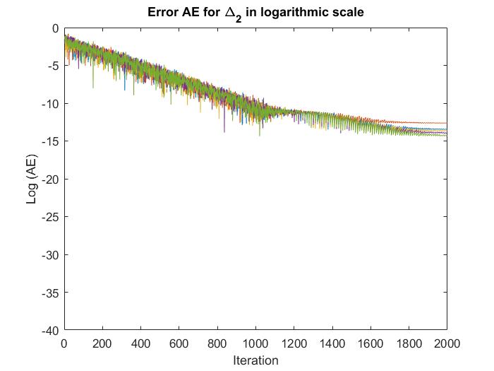
(a) Approximation error for $\Delta_{2}$ using Algorithm 2

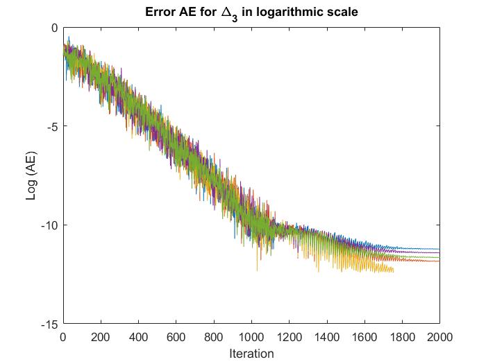
(b) Approximation error for $\Delta_{3}$ using Algorithm 2

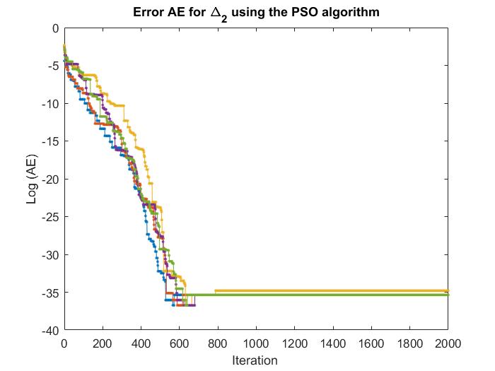
(c) Approximation error for $\Delta_{2}$ using PSO

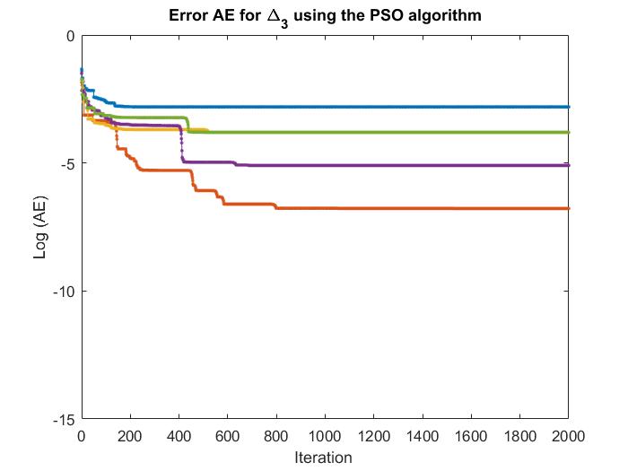
(d) Approximation error for $\Delta_{3}$ using PSO

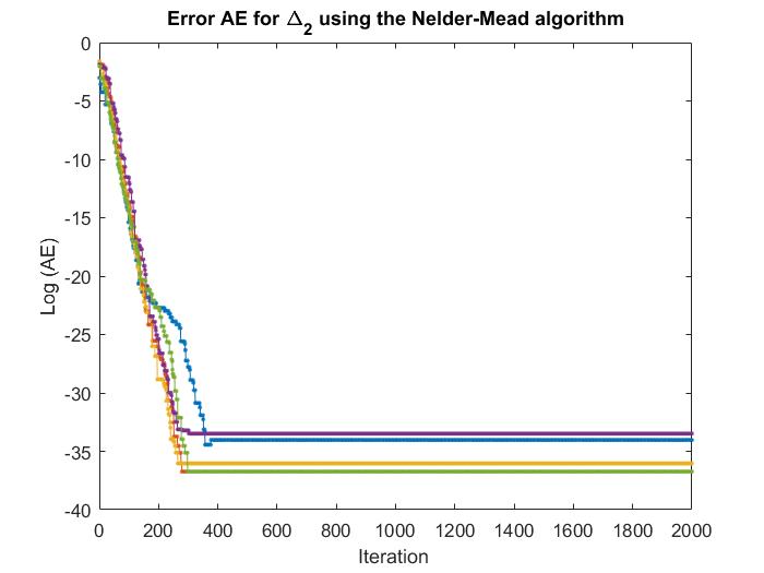
(e) Approximation error for $\Delta_{2}$ using Nelder-Mead

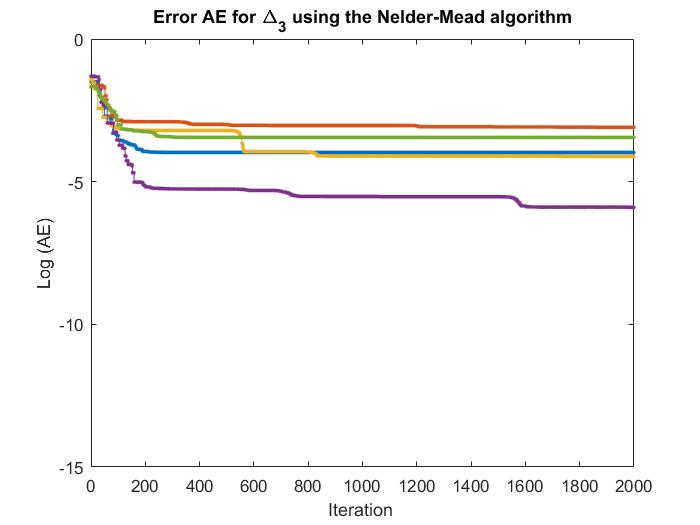
(f) Approximation error for $\Delta_{3}$ using Nelder-Mead

Figure 5.1: Plot of the absolute error ($AE$) generated by five executions using Algorithm 2, PSO and Nelder-Mead. Here, we use the logarithmic scale.

We now compare the proposed algorithm with the PSO and Nelder-Mead, for that, we run five different executions for the different algorithms. In Figure 5.2, we plot the absolute error $(AE)$ of approximating $\Delta_{2}$ and $\Delta_{3}$ for the iteration value $x_{n}$. Each color represents a different execution. The PSO and Nelder-Mead algorithms are implemented in the Manopt toolbox using default parameters. We implement the PSO algorithm with $40$ particles.
In addition, we test the proposed method to compute an approximation for the densities $\Delta_{4}$ and $\Delta_{5}$ using the previous setting. Although the problem remains unsolved in these dimensions, the best packing densities in the literature [21, 15] are $0.6168502750680849\cdots$ for $n=4$ and $0.4652576133092586…$ for $n=5$. Through the execution of the different algorithms, for both cases, the best packing density is obtained using the proposed methodology. In fact, the Algorithm 2 for the case $n=4$, gives an optimal packing density equal to $0.616825892885318$ and for $n=5$, gives $0.465218060094373$. Thus, as evidence, we observe that the proposed methodology outperforms the $PSO$ and $Nelder-Mead$ free derivative algorithms, for dimensions greater than $2$. We emphasize that the proposed methodology focuses on cases where in each iteration the only information available is a set of sample points lying in an unknown manifold. In such case, the solvers PSO and Nelder-Mead cannot be executed.

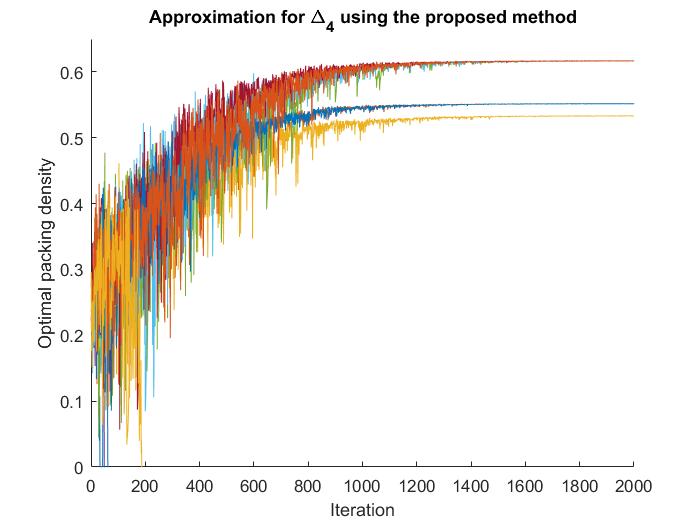
(a) Optimal packing density $\Delta_{4}$ using Algorithm 2

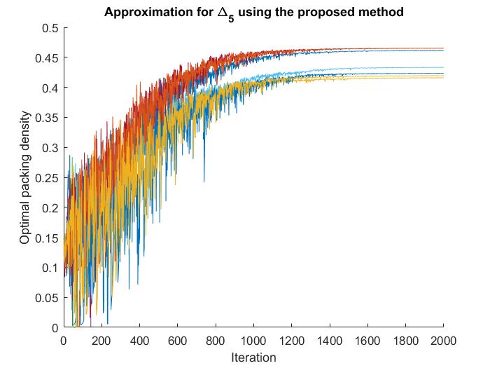
(b) Optimal packing density $\Delta_{5}$ using Algorithm 2

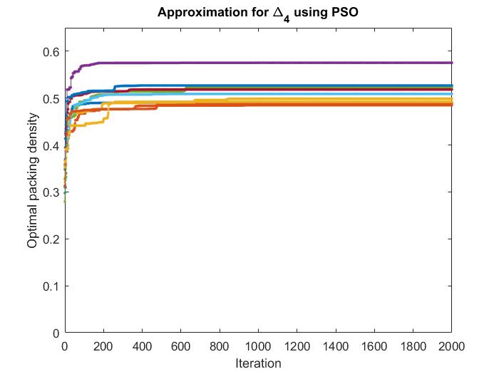
(c) Optimal packing density $\Delta_{4}$ using PSO

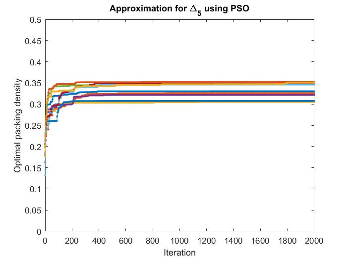
(d) Optimal packing density $\Delta_{5}$ using PSO

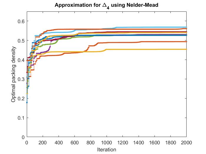
(e) Optimal packing density $\Delta_{4}$ using Nelder-Mead

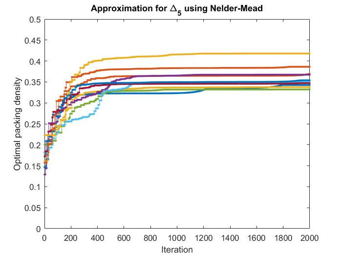
(f) Optimal packing density $\Delta_{5}$ using Nelder-Mead

Figure 5.2: Plot of the best packing density generated by ten executions using Algorithm 2, PSO, and Nelder-Mead.

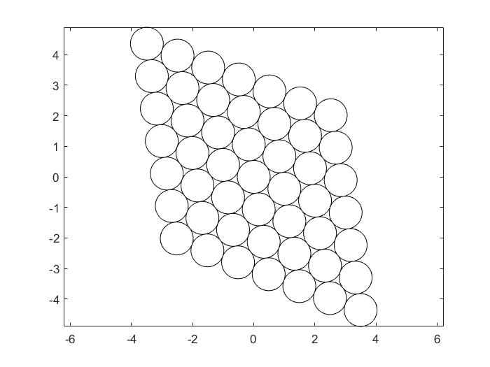
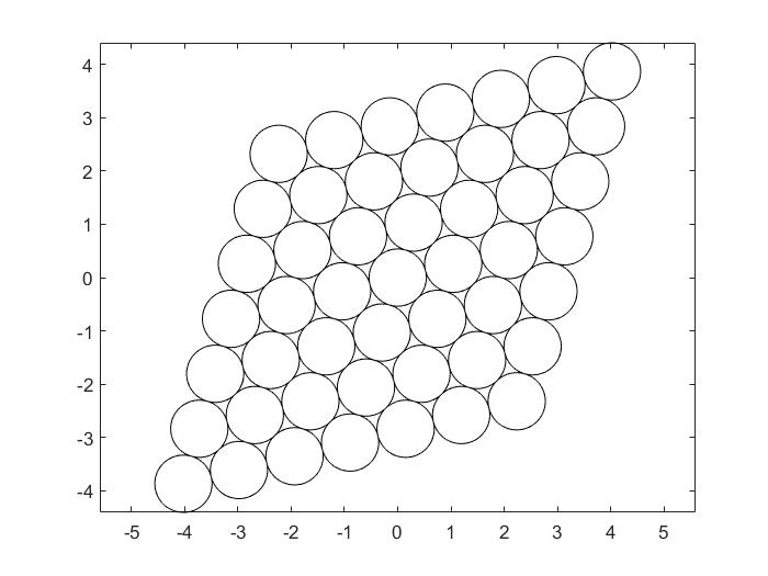
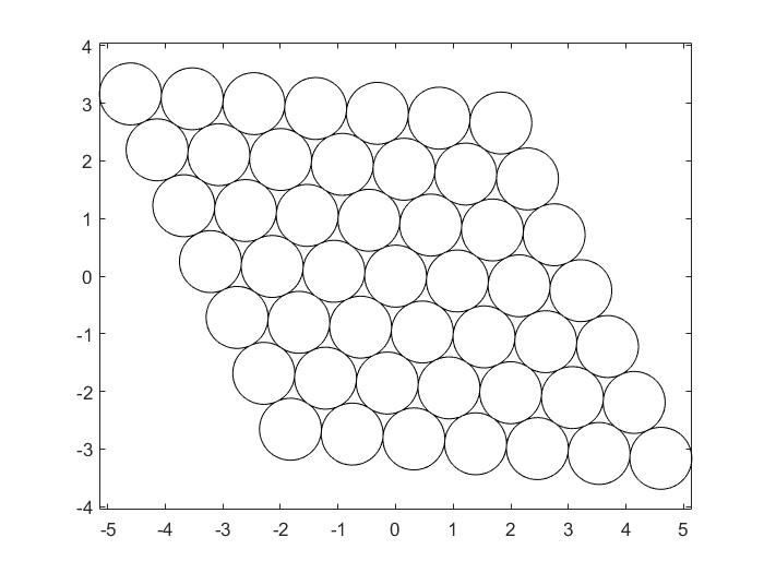
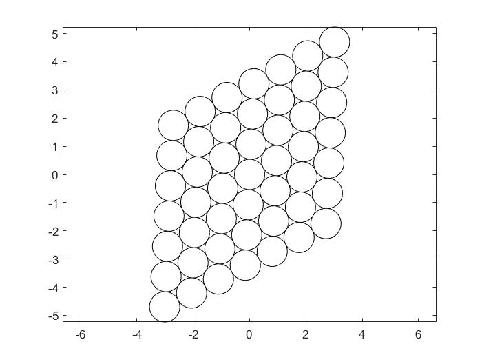
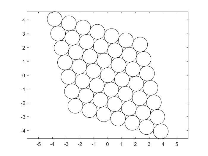
Figure 5.3: Plot of final lattice packing step of five executions to approximate the density $\Delta_{2}$.

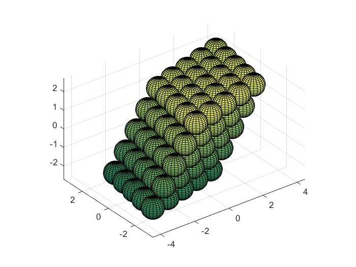
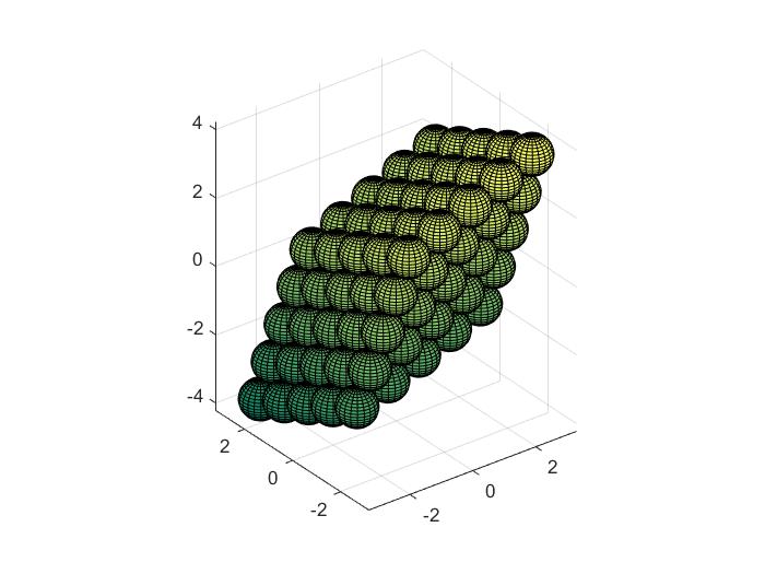
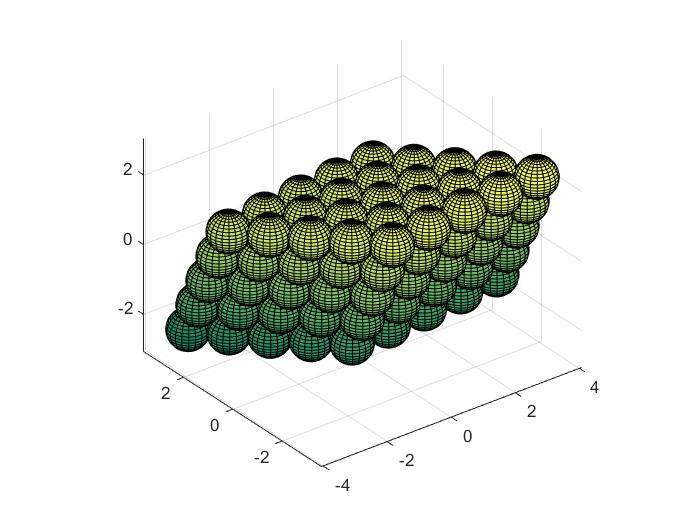
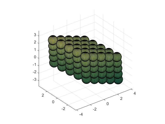
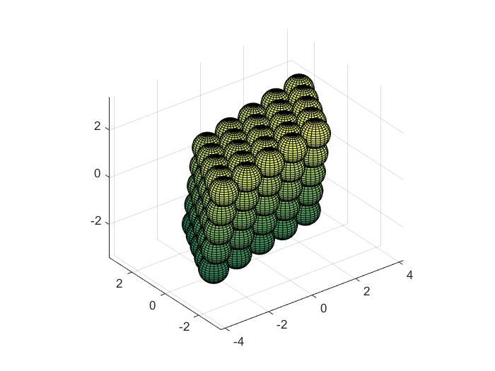
Figure 5.4: Plot of final lattice packing step of five executions to approximate the density $\Delta_{3}.$

5.2 Tomographic reconstruction from unknown random angles

Tomographic reconstruction is a widely studied problem in the field of inverse problems. Its goal is to reconstruct an object from its angular projections. This problem has many applications in medicine, optics and other areas. We refer the reader to Refs. [31, 23, 33, 39] for more details .

Classical reconstruction methods are based on the fact that the angular position is known. See Ref. [31]. In contrast, there are many cases for which the angles of the projections are not available, for instance, when the object is moving. The latter is a nonlinear inverse problem, which can be more difficult when compared to the classical linear inverse problem.

Now, we explain the problem in more details. Suppose that $f:\mathbb{R}^{2}\to\mathbb{R}_{\geq 0}$ describes the density of an object, and let $\theta$ be an angle. We define the one-dimensional tomographic projection over the angle $\theta$ as

$$\mathbb{P}_{\theta}f(x)=\int f(R_{\theta}(x,y))\,dy,$$

where $R_{\theta}(x,y)$ is the counterclockwise rotation of the two-dimensional vector $(x,y)$ with respect to the angle $\theta$. Since

$$\int|\mathbb{P}_{\theta_{i}}f(x)|\,dx=\int f(x,y)\,dydx,$$

thus, normalizing if necessary, we also assume that $\|\mathbb{P}_{\theta_{i}}f\|_{L^{1}}=1$. The problem under consideration consists in reconstructing the density $f$ with the knowledge of projections $\mathbb{P}_{\theta_{1}}f,\mathbb{P}_{\theta_{2}}f,\cdots\mathbb{P}_{\theta_{k}}f$, where the angles $\theta_{1},\theta_{2},\cdots\theta_{k}$ are unknown. If through some method the rotations are known, then we can obtain the density function $f$ using classical reconstruction methods.

In Ref. [17] an approach using the graph Laplacian is proposed to deal with this problem. However, the difficulty in using the previous approach is that it assumes a priori the knowledge of the distribution of the angles $\{\theta_{i}\}_{i=1}^{k}$. That is, it is necessary to assume the Euclidean distance between two consecutive angles. We use our methodology to tackle the latter problem, the road-map of our approach is established in Algorithm 3. Let $DS$ be the dataset defined as the set of all tomographic projections

$$DS=\{\mathbb{P}_{\theta_{i}}f\}_{i=1}^{k}.$$ (5.3)

If we assume that the density function $f$ has compact support, then a straightforward computation gives

$$\int\mathbb{P}_{\theta_{i}}f(x)\,x\,dx =\int\int\langle(x,y),(f(R_{\theta}(x,y),0))\rangle dxdy$$

$$=\int\int\langle(x,y),R_{\theta}(f(x,y),0))\rangle dxdy$$

$$=\langle\tilde{V},R_{\theta_{i}}\,(1,0)\rangle,$$ (5.4)

where $\tilde{V}$ is the two-dimensional vector

$$\tilde{V}=(\int\int xf(x,y)\,dxdy,\int\int yf(x,y)\,dxdy).$$

For practical purposes, we consider the discretization of the projection $\mathbb{P}_{\theta_{i}}f$ as the multidimensional vector given by

$$\overline{\mathbb{P}_{\theta_{i}}}f=(\mathbb{P}_{\theta_{i}}f(x_{1}),\mathbb{P}_{\theta_{i}}f(x_{2}),\cdots,\mathbb{P}_{\theta_{i}}f(x_{l})),$$

where $x_{1}<x_{2}<\cdots<x_{l}$ are equally spaced fixed points on the $x$ axis that describe the projection onto the angle $\theta_{i}$. See Figure 5.5.

Figure 5.5: Tomography of an object.

Let $X$ be the multidimensional vector

$$X=(x_{1},x_{2},\cdots,x_{l}).$$

The discretization of the integrals in Eq. (5.4) gives

$$\frac{1}{h}\,\langle\,\overline{\mathbb{P}_{\theta_{i}}}f,X\rangle\approx\langle\tilde{V},R_{\theta_{i}}\,(1,0)\rangle,$$ (5.5)

where $h$ is the distance between two consecutive points. Equation (5.5) allows to estimate, except for a possible sign and translation, the angle $\theta_{i}$. Namely, if the two-dimensional vector $\tilde{V}$ has angle $\tilde{\theta}$, then, we recover $\theta_{i}$ using the expression

$$\cos\,(\theta_{i}-\tilde{\theta})\approx\frac{1}{h\,\,\|\tilde{V}\|_{2}}\langle\overline{\mathbb{P}_{\theta_{i}}}f,X\rangle.$$ (5.6)

In this case, we use Eq. (5.5) to compute the value $\|\tilde{V}\|$ as

$$\|\tilde{V}\|_{2}\approx\max_{\theta_{i}}\left|\frac{1}{h}\langle\overline{\mathbb{P}_{\theta_{i}}}f,X\rangle\right|.$$ (5.7)

We remark that in this approach we do not compute the two-dimensional vector $\tilde{V}$, instead, we compute the norm $\|\tilde{V}\|$ using Eq. (5.7). Observe that to solve the optimization Problem in Eq.  (5.7) it is sufficient to assume that ${\theta_{i}}\in[0,\pi]$.

Once we solve the previous optimization problem, we use Eq. (5.5) to calculate the angle $\theta_{i}-\tilde{\theta}$. Observe that if we do not determine the sign of the $\theta_{i}-\tilde{\theta}$, then a flipping effect appears on the reconstructed object, resulting in an image with many artifacts. We apply our gradient estimates to determine the sign of the angle. For that, we assume that the angles are distributed on the interval $I=[0,\pi]$, and consider the numbers

$$m_{1}=\min_{i}|\theta_{i}-\tilde{\theta}|\quad\quad and\quad\quad M_{1}=\max_{i}|\theta_{i}-\tilde{\theta}|.$$ (5.8)

Since the maximum of the optimization problem in Eq. (5.7) is reached for some $\theta_{i}$, then $m_{1}=0$ or $M_{1}=\pi$. Without loss of generality, it is enough to consider the case $m_{1}=0$. In fact, if $M_{1}=\pi$, then we reflect the angles over the $y$-axis. Furthermore, changing the order if necessary we assume that

$$0=|\theta_{1}-\tilde{\theta}|<|\theta_{2}-\tilde{\theta}|<\cdots<|\theta_{k}-\tilde{\theta}|.$$ (5.9)

We observe that our dataset $(DS)$ defined as in Eq. (5.3) lies in the curve $c(I)$, which is parameterized by

$$c(\theta)=\mathbb{P}_{\theta}f,$$

and in our case this parametrization is unknown. The main idea in our algorithm is to use the gradient flow of the function $g$ on the manifold $c(I)$, where $g:c(I)\to\mathbb{R}$ is defined as

$$g(Y)=\frac{1}{h}\langle Y,X\rangle.$$ (5.10)

The importance of the gradient flow in our method lies in the fact that in a local neighborhood of the vector associated with the angle $0$, the gradient flow divides the dataset into two different clusters that determine the sign of the associated angles. This fact is proved using the approximation (5.6) and the fact that the derivative of $\it{cosine}$ is an odd function on the real line.

Before initializing our algorithm we divide the indices $\tilde{A}=\{i\}_{i=1}^{k}$ as follows. We select a fixed number $s$, which represents the size of the partition, and we consider the decomposition $k=us+r$, where $u$ and $r$ are non-negative integers with $r<s$. Then, we define the sets

$$\tilde{A}_{i}=\{is+1,is+2,\cdots,(i+1)s\},$$ (5.11)

for $i\in\{0,1,2,\cdots,q-1\}$, and

$$\tilde{A}_{q}=\tilde{A}\,\,\setminus\bigcup_{i=0}^{u-1}\tilde{A}_{i}.$$ (5.12)

We use the partition $\{\tilde{A}_{i}\}_{i=1}^{q}$ to represent the local geometry of the dataset. For that, we consider the subset $DS_{i}$ of $DS$, defined as

$$DS_{i}=\{\mathbb{P}_{\theta_{j}}f\,|j\in A_{i}\}.$$ (5.13)

The first step in our algorithm is to determine the sign of angles in a local neighborhood of $0$, for that, we use the diffusion-map algorithm to embed the dataset $\overline{DS}_{1}=DS_{1}\cup DS_{2}\cup DS_{3}$ into the two-dimensional space $\mathbb{R}^{2}$. We endow this embedded dataset with the counting measure. Once the dataset is embedded, we proceed to compute the approximation for $\overline{P}_{1}\tilde{g}$ as described in Algorithm 1. Here, we select the points $x_{1},x_{2},x_{3}\cdots x_{m}$ as the $m$ closest points to $x$. Since we only are interested in the direction induced by the gradient, then we propose to reduce the computational cost of the execution using the approximation

$$\overline{\mathcal{V}}=\sum_{i=1}^{m}(x_{i}-x)\,\,(\tilde{g}(x_{i})-\tilde{g}(x))\,\,e^{\frac{-\|x_{i}-x\|^{2}}{2}},$$ (5.14)

where, the function $\tilde{g}$ is such that for each two-dimensional embedded point $y\in\mathbb{R}^{2}$ associated with vector $Y\in DS$, the value of $\tilde{g}(x)$ is defined as

$$\tilde{g}(y)=g(Y).$$ (5.15)

The two-dimensional representation of the dataset allows determining the sign of the angles $\theta_{i}-\tilde{\theta}$ regarding the orientation of the flow generated by the function $\tilde{g}(y)$. This is done by observing that locally the set of gradient vectors associated with positive angles and the set of gradient vectors associated with negative angles are separated by a hyperplane. Since $\theta_{2}-\tilde{\theta}$ is the smallest nonzero angle, then we use its gradient to define a hyperplane that separates the sets mentioned above. To be more specific, we separate the sets according to the sign of the inner product of its gradient with the gradient associated with $\theta_{2}-\tilde{\theta}$. We remark that in the first step we only classify the sign of angles associated with points lying in $DS_{1}\cup DS_{2}$, to avoid instabilities generated by computing the gradient of the boundary points lying in $DS_{3}$.

The second step is to proceed inductively to determine the sign of the remaining angles as follows. Assume that for $2\leq i$ the sign of the angles associated with points lying in the set $DS_{i}$ is determined, and consider the dataset $\overline{DS}_{i}=DS_{i}\cup DS_{i+1}$. As in the first step, we use diffusion-maps to embed this dataset into $\mathbb{R}^{2}$. Observe that the function $g$ has not critical points on $\overline{DS}_{i}$. Then, the two-dimensional representation is divided at most into two clusters, for which each cluster represents the set of points with the same sign. We determine the sign of each cluster according to the sign of angles associated with points in $DS_{i}$ lying in the corresponding cluster. For practical purposes, we define the sign of each angle $\theta_{i}-\tilde{\theta}$ as the sign of the angle previously determined with the closest two-dimensional representation. We run this step until all the signs are determined. We summarize this reconstruction method in Algorithm 3. We remark that the choice of parameters $s$ and $m$ have to be modestly small to avoid instabilities in our algorithm.

input Tomographic projections $DS=\{Y_{i}\}_{i=1}^{k}$, where $Y_{i}=\mathbb{P}_{\theta_{i}}f$, size of the partition $s$.

1. Normalize the dataset $DS$ such that $\|\mathbb{P}_{\theta_{i}}f\|_{L^{1}}=1$ for all $i$.

2. Compute $\|\tilde{V}\|_{2}$ solving the optimization problem 5.7.

3. Determine the angles $\theta_{i}-\tilde{\theta}$ using Eq. (5.6).

4. Compute $M_{1}$ as in Eq. (5.8).

5. If $M_{1}=\pi$, then we proceed to reflect the angles $\tilde{\theta_{i}}$ over the $y$-axis.

6. Construct $DS_{i}$ following Eqs (5.11), (5.12), and (5.13).

7. Use the diffusion-map approach to embed the dataset $DS_{1}\cup DS_{2}\cup DS_{3}$ into $\mathbb{R}^{2}$.

8. Compute $\overline{P}_{1}\tilde{g}$ using the approximation (5.14), where $\tilde{g}$ is defined in Eqs. (5.10) and (5.15).

9. Determine the sign of the angles $\tilde{\theta_{i}}$ associated with points in $DS_{1}\cup DS_{2}$, according to the sign of the inner product of the associated gradient with the gradient associated with $\theta_{2}$.

10. for $j=2$ to $s$ do

    • Use the diffusion-map approach to embed the dataset $DS_{j}\cup DS_{j+1}$ into $\mathbb{R}^{2}$.

    • Determine the sign of each angle $\tilde{\theta_{i}}$ in $DS_{j+1}$ as the sign of angle previously determined with the closest two-dimensional representation.

11. end for

12. Reconstruct the signed angles.

Algorithm 3 Tomographic reconstruction from unknown random angles

The computational complexity of all the embeddings is $O(us^{3})$, which corresponds to the complexity of the eigenvalue decomposition. On the other hand, the complexity of all gradient computations is $O(s)$, and the computational complexity of the other procedures described in Algorithm 3 is $O(s)$. Thus, Algorithm 3 runs with a $O(us^{3})$ complexity which improves the $O(u^{3}s^{3})$ complexity of the algorithm proposed in Ref. [17].

We test our algorithm on the tomographic reconstruction of two objects. The first is the Shepp–Logan phantom, and the second is a computed tomography of a knee taken from Ref. [32]. See Figure 5.6. In this experiment, we generate $k=2\times 10^{3}$ random points uniformly distributed in $[0,\pi]$. The parameters used in Algorithm 3 are $s=20$, and $m=10$. The tomographic projections $\mathbb{P}_{\theta_{1}}f,\mathbb{P}_{\theta_{2}}f,\cdots\mathbb{P}_{\theta_{k}}f$ are computed using Matlab ‘s radon function. We add random noise to these projections, for that, we consider the dataset of the form

$$\mathbb{P}_{R_{i}}^{\varepsilon}f=\mathbb{P}_{R_{i}}f+\eta W,$$ (5.16)

where $W$ is a white noise. Our purpose is to recover the density $f$, using only the measurements $\mathbb{P}_{R_{i}}^{\varepsilon}f$, regardless of their respective angles.

To illustrate how Algorithm 3 works, we plot the two essential steps in the method. In Figure 5.7, we plot the first two-dimensional embedding and their respective gradient approximation defined in Eq. (5.14). Points with blue color are associated with positive angles and those with red color with negative angles. Furthermore, in Figure 5.8 , we plot the second two-dimensional embedding of our method. We observe that our method performs effectively in dividing the dataset into two different clusters according to the sign of the corresponding angle.

In Figures 5.9 and 5.10, we plot the reconstructed images of the Shepp–Logan phantom and the knee tomography, respectively. Here, the samples of the angles are uniformly distributed over $[0,\pi]$. We consider different levels of additive order error $\eta$ as represented in Eq. (5.16). We remark that we obtained similar results to those shown using multiple executions of our method. To measure the effectiveness of our method, we compare the $L^{2}$ error generated when our algorithm is implemented. The computed $L^{2}$ error is shown in Tables 1 and 2. Observing the computational error and image quality, we conclude that our reconstruction algorithm works efficiently with relatively low computational cost.

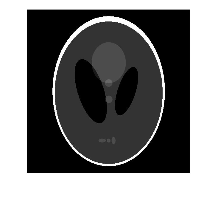
(a) Shepp–Logan phantom

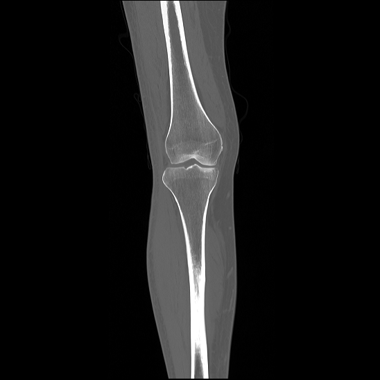
(b) Sample image of a knee

Figure 5.6: Picture of the Shepp–Logan phantom (a), and a knee sample image (b). Source for the latter Ref. [32].

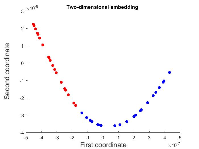
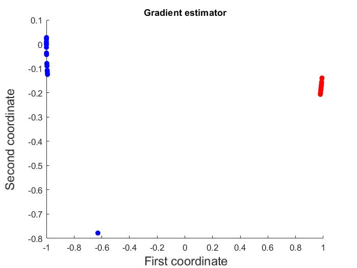
(a) Shepp–Logan phantom

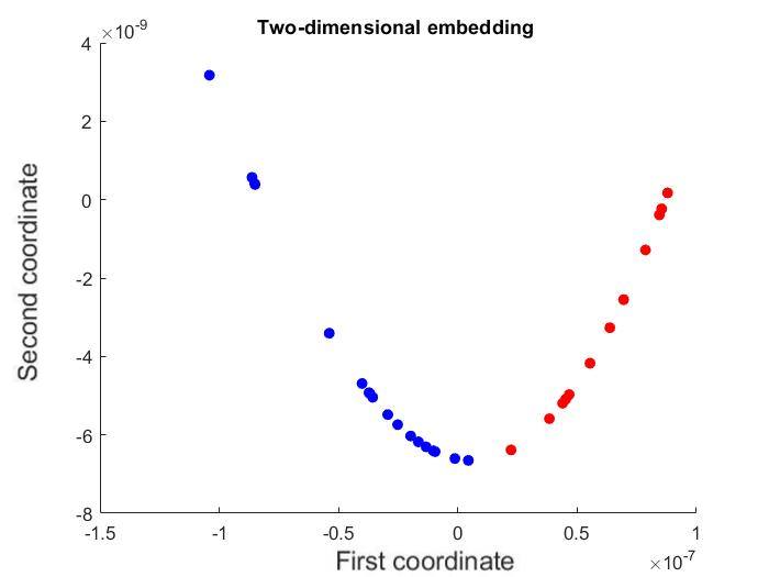
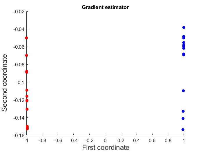
(b) Sample image of the knee

Figure 5.7: Plot of the first two-dimensional embedding (left), and their associated gradient approximation (right). In this experiment, the angle sample is uniformly distributed on $[0,\pi]$. Each color represents a different sign. Figure (a) corresponds to the Shepp–Logan phantom, and Figure (b) to the image of the knee.

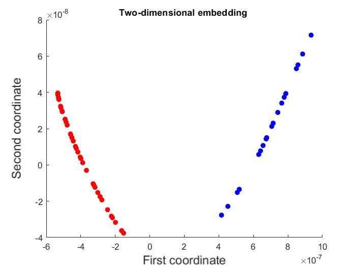
(a) Shepp–Logan phantom

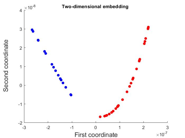
(b) Shepp–Logan phantom

Figure 5.8: Plot of the second two-dimensional embedding (left). Figure (a) corresponds to the Shepp–Logan phantom, and Figure (b) to the image of the knee.

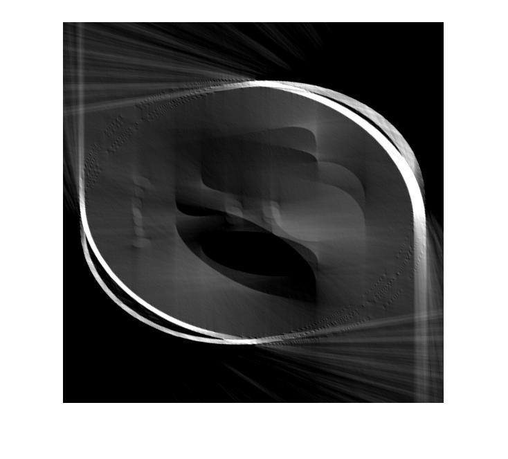
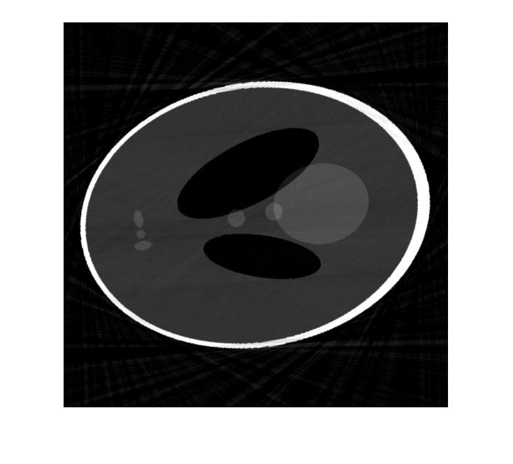
(a) $\eta=0$

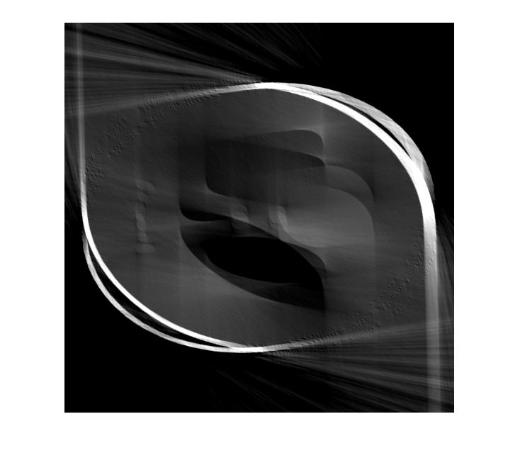
(b) $\eta=0.05$

(c) $\eta=0.1$

Figure 5.9: Reconstructed Shepp–Logan phantom for several additive errors $\eta$ as in Eq. (5.16). The images on the left are obtained without determining the sign of each angle, and the images on the right are obtained by implementing our algorithm.

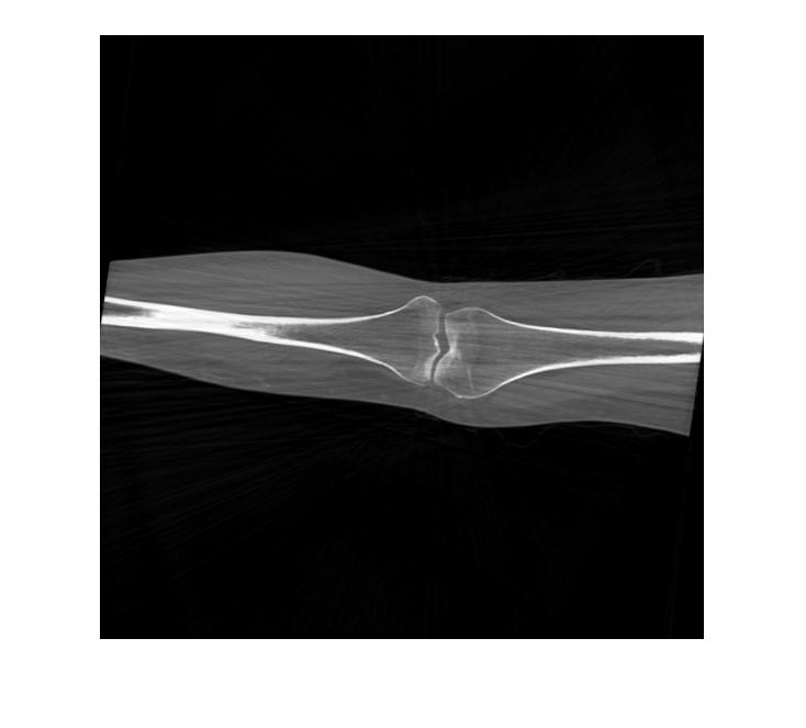
(a) $\eta=0$

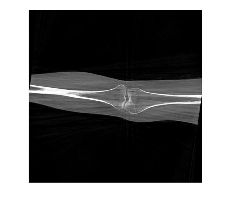
(b) $\eta=0.05$

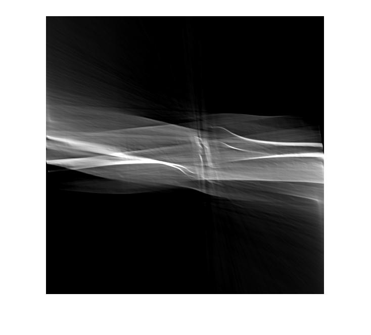
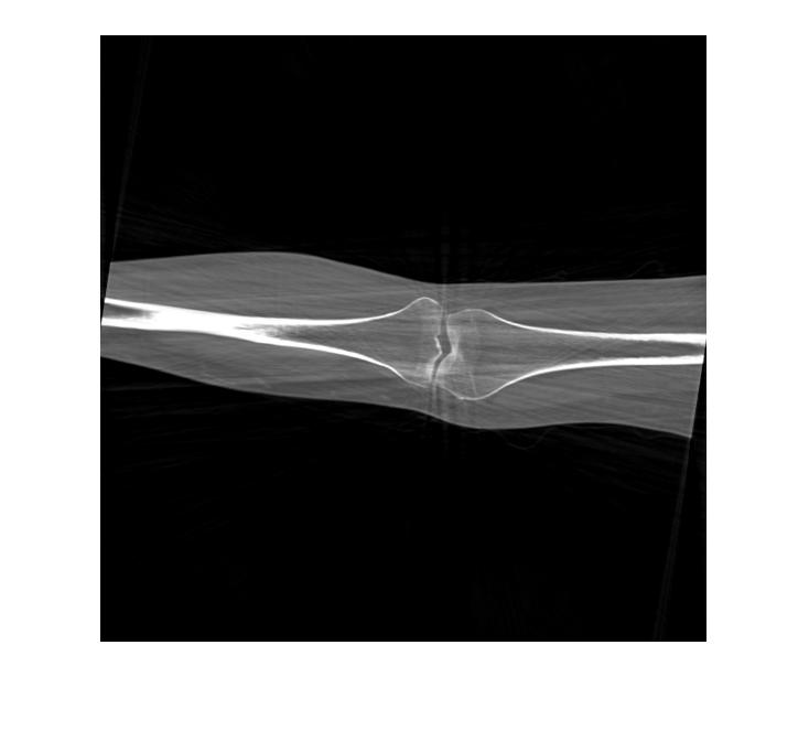
(c) $\eta=0.1$

Figure 5.10: Reconstructed knee tomography for several additive errors $\eta$ as in Eq. (5.16). The images on the left are obtained without determining the sign of each angle, and the images on the right are obtained by implementing our algorithm.

6 Conclusions

In this work, we recover the gradient operator defined on Riemannian submanifolds of the Euclidean space from random samples in a neighborhood of the point of interest. Our methodology is based on the estimates of the Laplace-Beltrami operator proposed in the diffusion maps approach. The estimates do not depend on the intrinsic parametrization of the submanifold. This feature is useful in cases where it is not feasible to identify the submanifold in which the dataset is lying. The proposed method gives a closed form of the gradient representation in the learning gradient theory. This improves the numerical implementation and the accuracy of the approximations. A natural continuation of the present work would be to incorporate information of the cotangent bundle and deal with a duality version of our results, in this case, the aforementioned approach would be very handy.

Value of $\eta$	With determination of the sign	Without determination of the sign
0	0.0814	0.2087
0.05	0.0816	0.2101
0.1	0.0824	0.2129

Table 1: Error of the reconstructed Shepp–Logan phantom. We use the $L^{2}$ norm to compute the errors. Here, the sample angles are uniformly distributed over $[0,\pi]$.

Value of $\eta$	With determination of the sign	Without determination of the sign
0	0.1001	0.1411
0.05	0.1053	0.1425
0.1	0.1114	0.1445

Table 2: Error of the reconstructed knee tomography . We use the $L^{2}$ norm to compute the errors. Here, the sample angles are uniformly distributed over $[0,\pi]$.

Furthermore, this circle of ideas could be conjoined with the techniques proposed in Ref. [41].

We conclude that the operator $\overline{P}_{t}f(x)$ locally approximates a smoothness version of the gradient of $f$. In fact, integrating by parts gives

$$\overline{P}_{t}f(x)=\frac{2t^{2}}{d_{t}(x)}\left(\int_{U(x,t^{\delta})}\nabla f(y)e^{\frac{-\|y-x\|^{2}}{2t^{2}}}dy+O(t^{\delta(d-1)})\right).$$

The question of whether $\overline{P}_{t}f(x)$ is a global approximation of some smoothness gradient remains open and it could be investigated in future work.

We apply our methodology in a step size algorithm as an optimization method on manifolds. This optimization method is effective in cases where it is difficult to compute the gradient of a function. As an application, we used our method to find an approximation to the sphere packing problem in dimensions 2 and 3, for the lattice packing case. Moreover, we use our approach to reconstruct tomographic images where the projected angles are unknown. The latter does not depend on a priory knowledge of the distribution of the angles, and its execution is computationally feasible.

A natural follow-up is to apply this methodology to the dimension reduction of high-dimensional datasets.

Due to the promising results obtained, another natural follow-up would be to implement our algorithm in the case of periodic lattice packing to obtain computational estimates for the sphere packing constant in several dimensions.

In addition, we plan to implement the gradient estimates in the reinforcement learning methodology, as well as implement the proposed method for other image reconstruction problems as well as integrate with other processing techniques such as the one described in Ref. [49].

Appendix A Numerical comparison with learning gradients

In this section, we verify the consistency of Proposition 4.1 and also compare the proposed algorithm with the learning gradient approximation [38]. We recall that given a sample set $\{x_{i}\}_{i}$ and a function $f$ in the manifold $\mathcal{M}$, the learning gradient method computes an approximation $\vec{f}$ for the gradient using the sample points $x_{i}$ as

$$\vec{f}=\sum_{i}C_{i}K_{t}(\cdot,x_{i}),$$ (A.1)

where $K$ is the Gaussian kernel $K_{t}(x,y)=e^{-\|x-y\|^{2}/2t^{2}}$, and the coefficients $C_{i}$ are determine by solving the optimal problem

$$\arg\max\sum_{i,j}w_{i,j}\left(f(x_{j})-f(x_{i})-\vec{f}(x_{i})\cdot(x_{j}-x_{i})\right)^{2}+\lambda\|\vec{f}\|_{L_{2}}^{2}$$ (A.2)

where $w_{i,j}=K(x_{i},x_{j})$. According to the theoretical results [38], to guarantee the convergence of the approximation the value for $\lambda$ is given by $\lambda=t^{d+3}$, where $d$ is the dimension of the manifold $\mathcal{M}$. The implementation of the difference between the Learning gradient and the proposed methodology lies in the fact that we compute a close form for the coefficients in the representation form (A.1) using the Markov normalization associated with Gaussian kernels. Thus, we avoid the costly time computation of solving the optimization problem (A.2). We test the learning gradient and the proposed methodology to compute the gradient of the function $f:M\to\mathbb{R}$ defined as

$$f(x)=<x,AA^{T}x>,$$

where $A$ is a squared matrix with random entries, and $<\cdot,\cdot>$ is the dot product in the Euclidean space. Here, the manifold $M$ is the curve $(c(t),c(t),c(t))\in\mathbb{R}^{9}$ parameterized by

$$c(t)=(\cos{2\pi t},\sin{2\pi t},\cos{4\pi t})\in\mathbb{R}^{3},$$

where $t\in[0,1]$ In this example, we consider random points on $t_{i}$ on $[0,1]$ and the set of sample points for which we compute the gradient approximation is defined as

$$x_{i}=(c(t_{i}),c(t_{i}),c(t_{i})).$$

We test both algorithms for different sample sizes $m$ and approximation parameters $t$. In Table 3, we compute the mean squared error (MSE) of each approximation method in a logarithmic scale. We remark that since this result is probabilistic, several executions were carried out to obtain similar results without altering the conclusions concerning the tolerance of the approximation involving the several parameters. In this experiment, we use $\delta=0.9$ and the parameter $t$ modestly small. Observe that for a fixed $t$, the MSE error decreases when the number of sample points $m$ increases, which is consistent with the result of Proposition 4.1. In addition, observe that the proposed methodology gives a less MSE error than the learning gradient method. This fact shows the consistency of the method with the theoretical development in this article.

$t$	$m$	Proposed methodology	Learning gradient
1	100	4.13	4.8
1	200	4.04	5.27
1	300	3.8	5.63
1	400	3.99	5.07
0.5	100	3.23	5.51
0.5	200	3.69	5.72
0.5	300	3.25	5.4
0.5	400	3.41	5.68
0.1	100	2.45	5.41
0.1	200	2.98	6.38
0.1	300	2.66	5.95
0.1	400	2.28	6.02
0.05	100	3.11	4.93
0.05	200	3.28	5.91
0.05	300	2.4	5.1
0.05	400	2.14	5.94

Table 3: Mean squared error of the gradient approximation for the proposed method and the learning gradient in a logarithm scale. Here, $m$ is the number of sample points, $t$ is the approximation parameter

Appendix B Review of differential geometry

We review some facts of differential geometry. We refer the reader to Ref. [24] for a more detailed description. Given an interior point $x\in\mathcal{M}$, there exists a positive real number $\varepsilon$ such that the map $\psi=\exp_{x}\circ\,T:B(0,\varepsilon)\subset\mathbb{R}^{d}\to\mathcal{M}$ is a local chart. Here, $\exp_{x}$ is the exponential map at the point $x$, and $T:\mathbb{R}^{d}\to T_{x}\mathcal{M}$ is a rotation from $\mathbb{R}^{d}$ onto $T_{x}\mathcal{M}$, both sets considered subsets of $\mathbb{R}^{n}$. The chart $\psi$ defines the normal coordinates at point $x$.

Given a smooth function $f\in C^{\infty}(\mathcal{M})$, the gradient operator $\nabla f(x)\in T_{x}\mathcal{M}$ is given in normal coordinates by

$$\nabla f(x)=\sum_{i=1}^{d}\frac{\partial f}{\partial x_{i}}T(e_{i}).$$

Here, $e_{i}$ is the standard basis in $\mathbb{R}^{d}$. Now, we recall some estimates that use normal coordinates that are useful when estimating approximations for differential operators. The Taylor series of $\psi$ around the point $0$ is given by

$$\psi(v)=x+T(v)+\frac{1}{2}D^{2}\psi_{0}(v,v)+O(\|v\|^{3}).$$ (B.1)

Let $v\in B(0,\varepsilon)\subset\mathbb{R}^{d}$, and consider the geodesic $\gamma_{T(v)}$, with initial tangent vector $T(v)\in T_{x}\mathcal{M}$, then using Estimate (B.1) we obtain

$$\gamma_{T(v)}(t)=x+T(v)\,t+\frac{1}{2}D^{2}\psi_{0}\,(v,v)t^{2}+O(\|v\|^{3})t^{3}.$$

Since the covariant derivative of a geodesic vanishes, then $\gamma^{\prime\prime}_{{T(v)}}$ is orthogonal to $T_{x}\mathcal{M}$. Thus, we have the following estimates

$$\|\psi(v)-x\|^{2}=\|T(v)\|^{2}+O(\|v\|^{4}),$$ (B.2)

and

$$\mathcal{P}_{x}(\psi(v)-x)=T(v)+O(\|v\|^{3}),$$ (B.3)

where $\mathcal{P}_{x}$ is the orthogonal projection on $T_{x}\mathcal{M}$. Using the Estimates (B.2) and (B.3), we obtain that there exist positive constants $M_{1}$ and $M_{2}$ such that for $\|v\|$ small

$$\|v\|-M_{2}\|v\|^{3}\leq\|\psi(v)-x\|\leq M_{1}\|v\|.$$

Thus, if $\|v\|^{2}\leq\frac{1}{2M2}$ we have

$$\frac{1}{2}\|v\|\leq\|\psi(v)-x\|\leq M_{1}\|v\|.$$

This says that for $t$ small

$$B(0,t/{M_{1}})\subseteq\psi^{-1}(U(x,t^{\delta}))\subseteq B(0,2t).$$ (B.4)

Appendix C Expansion of the gradient operator

Here, we show the technical details of the proof of Theorem 2.1. The main idea is to use the Taylor expansion of the function $f$ around the point $x$.

Lemma C.1.

Assume that $\frac{1}{2}<\delta<1$, and let $K:\mathcal{M}\times\mathcal{M}\to\mathbb{R}^{m}$ be a vector value kernel. Define

$$P_{t}(x)=\int_{U(x,t^{\delta})}K(x,y)\,e^{\frac{-\|y-x\|^{2}}{2t^{2}}}dy,$$

where $U(x,t^{\delta})$ is defined as in Eq. (2.1). Assume that for $t$ small, the function $\psi:B(0,2t^{\delta})\to\mathcal{M}$ defines normal coordinates in a neighborhood of $x$, and let $S$ be a vector value function defined in $\mathbb{R}^{d}$ such that

$$K(x,\psi(v))-S(v)=O(\|v\|^{r}),$$

and

$$K(x,y)=O(\|x-y\|^{s}).$$

Then, we have

$$P_{t}(x)=O((e^{C_{2}t^{4\delta-2}}-1)t^{s+d}+t^{r+d})+\int_{\psi^{-1}(U(x,t^{\delta}))}S(v)\,e^{\frac{-\|T(v)\|^{2}}{2t^{2}}}dv.$$

Proof.

Using Eq. (B.4), we assume that for $t$ small, the set $U(x,t^{\delta})$ lies in the image of a normal chart $\psi:B(0,2t^{\delta})\to\mathcal{M}$ centered in $x$. Thus,

$$\begin{array}[]{rcl}\int_{U(x,t^{\delta})}K(x,y)\,e^{\frac{-\|y-x\|^{2}}{2t^{2}}}dy&=&\int_{\psi^{-1}(U(x,t^{\delta}))}K(x,\psi(v))e^{\frac{-\|\psi(v)-x\|^{2}}{2t^{2}}}dv\\ &=&\int_{\psi^{-1}(U(x,t^{\delta}))}K(x,\psi(v))(e^{\frac{-\|\psi(v)-x\|^{2}}{2t^{2}}}-e^{\frac{-\|T(v)\|^{2}}{2t^{2}}})dv\\ &+&\int_{\psi^{-1}(U(x,t^{\delta}))}(K(x,\psi(v))-S(v))e^{\frac{-\|T(v)\|^{2}}{2t^{2}}}dv\\ &+&\int_{\psi^{-1}(U(x,t^{\delta}))}S(v)\,e^{\frac{-\|\mathbb{T}(v)\|^{2}}{2t^{2}}}dv.\end{array}$$

We now estimate

$$A=\int_{\psi^{-1}(U(x,t^{\delta}))}K(x,\psi(v))(e^{\frac{-\|\psi(v)-x\|^{2}}{2t^{2}}}-e^{\frac{-\|T(v)\|^{2}}{2t^{2}}})dv.$$

Using Eq. (B.2), and the inequality $|e^{x}-1|\leq e^{|x|}-1$ we obtain

$$\begin{array}[]{rcl}|e^{\frac{-\|\psi(v)-x\|^{2}}{2t^{2}}}-e^{\frac{-\|T(v)\|^{2}}{2t^{2}}}|&=&e^{\frac{-\|T(v)\|^{2}}{2t^{2}}}|e^{\frac{O(\|v\|^{4})}{2t^{2}}}-1|\\ &\leq&e^{\frac{-\|T(v)\|^{2}}{2t^{2}}}(e^{\frac{C_{1}\|v\|^{4}}{2t^{2}}}-1).\end{array}$$

Therefore, by Equation (B.4) we obtain

$$\begin{array}[]{rcl}\|A\|&\leq&C_{3}\,\,t^{s}(e^{C_{2}t^{4\delta-2}}-1)t^{d}\int_{\mathbb{R}^{d}}\|v\|^{s}e^{-\|v\|^{2}/2}dv\\ &=&O((e^{C_{2}t^{4\delta-2}}-1)t^{s+d}).\end{array}$$

On the other hand, by assumption we have

$$\int_{\psi^{-1}(U(x,t^{\delta}))}(K(x,\psi(v))-S(v))e^{\frac{-\|T(v)\|^{2}}{2t^{2}}}dv=O(t^{r+d}\,).$$

∎

Lemma C.2.

Under the same assumptions of Lemma C.1, we define

$$E=\int_{\psi^{-1}(U(x,t^{\delta}))}Q(v)e^{\frac{-\|T(v)\|^{2}}{2t^{2}}}g(v)dv,$$

where $g$ is a smooth function and $Q$ is a homogeneous polynomial of degree $l$. Then, we have

$$E=\int_{\mathbb{R}^{d}}Q(v)e^{\frac{-\|T(v)\|^{2}}{2t^{2}}}(g(0)+\sum\frac{\partial g}{\partial v_{i}}(0)v_{i})dv\,+O(t^{d+l}e^{-M_{2}t^{2(\delta-1)}}+t^{d+2+l}).$$

Proof.

Using the Taylor expansion of $g$ around $0$ we have

$$E=\int_{\psi^{-1}(U(x,t^{\delta}))}Q(v)e^{\frac{-\|T(v)\|^{2}}{2t^{2}}}(g(0)+\sum\frac{\partial g}{\partial v_{i}}(0)\,v_{i}+O(\|v\|^{2}))dv.$$

Let $B$ be defined as

$$B=\|\int_{\mathbb{R}^{d}\setminus\psi^{-1}(U(x,t^{\delta}))}Q(v)e^{\frac{-\|T(v)\|^{2}}{2t^{2}}}(g(0)+\sum\frac{\partial g}{\partial v_{i}}(0)\,v_{i})dv\|.$$

Using Eq. (B.4) and the fast decay of the exponential function, we obtain that

$$B\leq C_{4}t^{d+l}e^{-M_{2}t^{2(\delta-1)}}\int_{\mathbb{R}^{d}\setminus B(0,t^{\delta-1}/M_{1})}P(\|v\|)e^{\frac{-\|T(v)\|^{2}}{4}}dv.$$

for a certain polynomial $P$. Therefore, we have

$$B=O(t^{d+l}e^{-M_{2}t^{2(\delta-1)}}),$$

for a proper constant $M_{2}$. Finally, we observe that

$$\int_{\psi^{-1}(U(x,t^{\delta}))}Q(v)e^{\frac{-\|T(v)\|^{2}}{2t^{2}}}O(\|v\|^{2})dv=O(t^{d+2+l}).$$

∎

We recall the following computations related to the moments of the normal distribution that are useful in proving Theorem 2.1. For all index $i$

$$\int_{\mathbb{R}^{d}}v_{i}e^{\frac{-\|T(v)\|^{2}}{2t^{2}}}dv=0,$$

and

$$\int_{\mathbb{R}^{d}}v_{i}^{2}e^{\frac{-\|T(v)\|^{2}}{2t^{2}}}dv=(2\pi)^{\frac{d}{2}}\,t^{d+2},$$

moreover, if $i\neq j$ then

$$\int_{\mathbb{R}^{d}}v_{i}\,v_{j}e^{\frac{-\|T(v)\|^{2}}{2t^{2}}}dv=0.$$

Lemma C.3.

Under the same assumptions of Lemmas C.1 and C.2 we have

$$d_{t}(x)=(2\pi)^{\frac{d}{2}}t^{d}+O(t^{d+4\delta-2}).$$ (C.1)

Proof.

We apply Lemmas C.1 and C.2 to the functions $K(x,y)=1$, $S(v)=1$, $Q(v)=1$, and $g(x)=1$. We use the parameters $r=2$, $s=0$ and $l=0$. Using the exponential decay we obtain the following estimate

$$d_{t}(x)=(2\pi)^{\frac{d}{2}}t^{d}+O(t^{d+4\delta-2}).$$

∎

Proof of Theorem 2.1.

We apply Lemmas C.1 and C.2 to the functions $K(x,y)=(y-x)(f(y)-f(x))$, $S(v)=T(v)(f(\psi(v))-f(x))=\sum v_{i}(f(\psi(v))-f(x))T(e_{i})$ , $Q(v)=v_{i}$ and $g(v)=(f(\psi(v))-f(x))$. Since $\psi(v)-x-T(v)=O(\|v\|^{2})$ and $f(\psi(v))-f(x)=O(\|v\|^{1})$, then the parameters that we use are $r=3$, $s=2$ and $l=1$. Again, using the exponential decay we have that

$$\int_{U(x,t^{\delta})}\overline{K}(x,y)\,e^{\frac{-\|y-x\|^{2}}{2t^{2}}}dy=(2\pi)^{\frac{d}{2}}\,t^{d+2}\sum\frac{\partial f}{\partial v_{i}}(0)\,T(e_{i})+O(t^{d+4\delta}).$$ (C.2)

Finally we use Eq. (C.1) of Lemma C.3 to conclude the result. ∎

Received xxxx 20xx; revised xxxx 20xx.

E-mail address, Alvaro Almeida Gomez: alvaro.gomez@ku.ac.ae

E-mail address, Antônio J. Silva Neto: ajsneto@iprj.uerj.br

E-mail address, Jorge P. Zubelli: zubelli@gmail.com

References

- [1] P. Absil, R. Mahony, and R. Sepulchre, Optimization Algorithms on Matrix Manifolds, vol. 78, Princenton University Press, 2008.
- [2] R. L. Adler, J. Dedieu, J. Y. Margulies, M. Martens, and M. Shub, Newton’s method on riemannian manifolds and a geometric model for the human spine, Ima Journal of Numerical Analysis, (2002).
- [3] A. Almeida Gomez, A. Silva Neto, and J. Zubelli, Diffusion representation for asymmetric kernels, Applied Numerical Mathematics, 166 (2021), pp. 208–226.
- [4] S. Basu and Y. Bresler, Feasibility of tomography with unknown view angles, in Proceedings 1998 International Conference on Image Processing. ICIP98, 1998, pp. 15–19 vol.2.
- [5] A. Bensoussan and J. Menaldi, Difference equations on weighted graphs, Journal of Convex Analysis, 12 (2003).
- [6] A. Berahas, L. Cao, K. Choromanski, and K. Scheinberg, A theoretical and empirical comparison of gradient approximations in derivative-free optimization, Foundations of Computational Mathematics, (2021).
- [7] A. Bloch, Hamiltonian and gradient flows, algorithms and control, vol. 3, American Mathematical Soc., 1994.
- [8] J. Bonnans, J. Gilbert, C. Lemaréchal, and C. Sagastizabal, Numerical Optimization – Theoretical and Practical Aspects, Springer, 01 2006.
- [9] M. A. A. Bortoloti, T. A. Fernandes, O. P. Ferreira, and J. Yuan, Damped newton’s method on riemannian manifolds, Journal of Global Optimization, 77 (2020).
- [10] N. Boumal and B. Mishra, Manopt Toolbox, Sep. 5, 2021. https://github.com/NicolasBoumal/manopt.
- [11] N. Boumal, B. Mishra, P.-A. Absil, and R. Sepulchre, Manopt, a matlab toolbox for optimization on manifolds, Journal of Machine Learning Research, 15 (2014), pp. 1455–1459.
- [12] X. Bresson and T. Chan, Fast dual minimization of the vectorial total variation norm and applications to color image processing, Inverse Problems and Imaging, 2 (2008), pp. 455–484.
- [13] F. Bullo and K. Fujimoto, Lagrangian and Hamiltonian Methods For Nonlinear Control 2006: Proceedings from the 3rd IFAC Workshop, Nagoya, Japan, July 2006, Lecture Notes in Control and Information Sciences, Springer Berlin Heidelberg, 2007.
- [14] C. Chapman, Implementation of shortest vector of a lattice using exhaustive enumeration, 2018 (accessed December 1, 2021). https://github.com/enthdegree/lenum.m.
- [15] H. Cohn, D. de Laat, and A. Salmon, Three-point bounds for sphere packing, 2022.
- [16] H. Cohn, A. Kumar, S. Miller, D. Radchenko, and M. Viazovska, The sphere packing problem in dimension 24, Annals of Mathematics, 185 (2016).
- [17] R. Coifman, Y. Shkolnisky, F. Sigworth, and A. Singer, Graph laplacian tomography from unknown random projections, IEEE Transactions on Image Processing, 17 (2008), pp. 1891–1899.
- [18] R. R. Coifman and M. J. Hirn, Diffusion maps for changing data, Applied and Computational Harmonic Analysis, 36 (2014), pp. 79 – 107.
- [19] R. R. Coifman and S. Lafon, Diffusion maps, Applied and Computational Harmonic Analysis, 21 (2006), pp. 5 – 30. Special Issue: Diffusion Maps and Wavelets.
- [20] R. R. Coifman, S. Lafon, A. B. Lee, M. Maggioni, B. Nadler, F. Warner, and S. W. Zucker, Geometric diffusions as a tool for harmonic analysis and structure definition of data: Diffusion maps, Proceedings of the National Academy of Sciences, 102 (2005), pp. 7426–7431.
- [21] J. H. Conway, S. N. J. A., and E. Bannai, Sphere packings, lattices and groups, Springer-Verlag, 1993.
- [22] I. Daubechies, G. Teschke, and L. Vese, Iteratively solving linear inverse problems under general convex constraints, Inverse Problems and Imaging, 1 (2007), pp. 29–46.
- [23] S. Deans, The Radon Transform and Some of Its Applications, A Wiley-Interscience publication, Wiley, 1983.
- [24] M. do Carmo, Riemannian Geometry, Mathematics (Boston, Mass.), Birkhäuser, 1992.
- [25] L. M. G. Drummond and B. F. Svaiter, A steepest descent method for vector optimization, Journal of Computational and Applied Mathematics, 175 (2005), pp. 395–414.
- [26] A. Edelman, T. A. Arias, and S. Smith, The geometry of algorithms with orthogonality constraints, SIAM J. Matrix Anal. Appl., 20 (1998), pp. 303–353.
- [27] L. Evans, Partial differential equations, American Mathematical Society, Providence, R.I., 2010.
- [28] E. Gobet, G. Liu, and J. P. Zubelli, A nonintrusive stratified resampler for regression Monte Carlo: application to solving nonlinear equations, SIAM J. Numer. Anal., 56 (2018), pp. 50–77.
- [29] H. Groemer, Existenzsätze für lagerungen in metrischen räumen, Monatshefte Fur Mathematik, 72 (1968), pp. 325–334.
- [30] T. Hales, A proof of the kepler conjecture, Annals of Mathematics, 162 (2005), pp. 1065–1185.
- [31] G. Herman, Fundamentals of Computerized Tomography: Image Reconstruction from Projections, Advances in Computer Vision and Pattern Recognition, Springer London, 2009.
- [32] J.Cheng, Tomographic image of a knee. https://radiopaedia.org/cases/normal-ct-knee-1. Accessed: 2021-11-01.
- [33] A. Kak and M. Slaney, Principles of Computerized Tomographic Imaging, Society for Industrial and Applied Mathematics, 2001.
- [34] G. Malajovich and J. P. Zubelli, On the geometry of graeffe iteration, Journal of Complexity, 17 (2001), pp. 541–573.
- [35] , Tangent graeffe iteration., Numerische Mathematik, 89 (2001), pp. 749–782.
- [36] E. Malhotra and A. Rajwade, Tomographic reconstruction from projections with unknown view angles exploiting moment-based relationships, in 2016 IEEE International Conference on Image Processing (ICIP), 2016, pp. 1759–1763.
- [37] S. Mukherjee and Q. Wu, Estimation of gradients and coordinate covariation in classification, Journal of Machine Learning Research, 7 (2006), pp. 2481–2514.
- [38] S. Mukherjee, Q. Wu, and D.-X. Zhou, Learning gradients on manifolds, Bernoulli, 16 (2010).
- [39] F. Natterer, The Mathematics of Computerized Tomography, Society for Industrial and Applied Mathematics, 2001.
- [40] C. Olds, A. Lax, G. Davidoff, and G. Davidoff, The Geometry of Numbers, Mathematical Association of America, 2000.
- [41] D. Pozharskiy, N. Wichrowski, A. B. Duncan, G. A. Pavliotis, and I. G. Kevrekidis, Manifold learning for accelerating coarse-grained optimization, Journal of Computational Dynamics, 7 (2020), pp. 511–536.
- [42] H. Sato, Riemannian Optimization and Its Applications, Springer, 2021.
- [43] C. Schnorr and M. Euchner, Lattice basis reduction: Improved practical algorithms and solving subset sum problems, Mathematical programming, 66 (1994), pp. 181–199.
- [44] M. Shub and S. Smale, Complexity of bézout’s theorem. i. geometric aspects, Journal of the American Mathematical Society, (1993).
- [45] S. Smale, Newton’s method estimates from data at one point, in The Merging of Disciplines: New Directions in Pure, Applied, and Computational Mathematics, Springer New York, 1986.
- [46] S. Smith, Optimization techniques on riemannian manifolds, ArXiv, abs/1407.5965 (2014).
- [47] G. Teschl, Ordinary differential equations and dynamical systems, American Mathematical Society, (2008).
- [48] M. Viazovska, The sphere packing problem in dimension 8, Annals of Mathematics, 185 (2016).
- [49] J. P. Zubelli, R. Marabini, C. O. S. Sorzano, and G. T. Herman, Three-dimensional reconstruction by Chahine’s method from electron microscopic projections corrupted by instrumental aberrations, Inverse Problems, 19 (2003), pp. 933–949.