Population properties of neutron stars in the coalescing compact binaries

Abstract

We perform a hierarchical Bayesian inference to investigate the population properties of the coalescing compact binaries involving at least one neutron star (NS). With the current gravitational wave (GW) observation data, we can rule out none of the Double Gaussian, Single Gaussian, and Uniform NS mass distribution models, though a specific Double Gaussian model inferred from the Galactic NSs is found to be slightly more preferred. The mass distribution of black holes (BHs) in the neutron star-black hole (NSBH) population is found to be similar to that in the Galactic X-ray binaries. Additionally, the ratio of the merger rate densities between NSBHs and BNSs is estimated to be $\sim 3:7$. The spin properties of the binaries, though constrained relatively poorly, play nontrivial role in reconstructing the mass distribution of NSs and BHs. We find that a perfectly aligned spin distribution can be ruled out, while a purely isotropic distribution of spin orientation is still allowed. To evaluate the feasibility of reliably determining the population properties of NSs in the coalescing compact binaries with upcoming GW observations, we perform simulations with a mock population. We find that with 100 detections (including BNSs and NSBHs) the mass distribution of NSs can be well determined, and the fraction of BNSs can also be accurately estimated.

1 Introduction

Recently, the observations of gravitational wave (GW) signals from two neutron star-black hole (NSBH) coalescences, i.e., GW200105 and GW200115, have been reported by LIGO/Virgo/KAGRA Collaboration (LVKC; Abbott et al., 2021a). These two events are also the first confident observations of NSBH binaries in the Universe, although previously the modeling of the kilonova emission of hybrid GRB 060614 was also strongly in favor of an NSBH merger origin (Yang et al., 2015; Jin et al., 2015). Since the first successful detection of GW (Abbott et al., 2016) in 2015, about $\sim 50$ compact binary coalescences (CBCs) have been formally reported (Abbott et al., 2021b), including $\sim 45$ events from binary black hole (BBH) coalescences and several mergers involving at least one neutron star (e.g., Abbott et al., 2017, 2020a, 2020b, 2020c). Very recently, The LIGO Scientific Collaboration et al. (2021) releases a deep extended catalog, which reports another 8 new events. With a rapidly increasing sample of GW events, our understanding of the population properties of the stellar BHs in the Universe has been advanced (e.g., Talbot & Thrane, 2017; Abbott et al., 2019a; Fishbach & Holz, 2020; Abbott et al., 2021c; Wang et al., 2021b; Li et al., 2021; Kimball et al., 2021; Tiwari & Fairhurst, 2021; Kimball et al., 2021; Galaudage et al., 2021b), and some formation/evolution processes of the compact binaries are being revealed (e.g., Kimball et al., 2020, 2021; Safarzadeh & Wysocki, 2021; Baxter et al., 2021; Tang et al., 2021b; Mapelli et al., 2021; Wang et al., 2021a). However, due to the limited observation of NSBH and BNS mergers up to now, the population properties of these kinds of coalescence systems are hard to probe. Moreover, Tang et al. (2020) found that the misclassification of BBH into NSBH makes it more challenging to reconstruct the mass function of the BHs.

Thanks to the observation of Galactic radio pulsars, a large number of NS masses have been measured (Valentim et al., 2011; Antoniadis et al., 2016; Özel & Freire, 2016; Alsing et al., 2018; Farrow et al., 2019; Rocha et al., 2019; Shao et al., 2020a; Galaudage et al., 2021a; Farr & Chatziioannou, 2020). The mass distribution of these Galactic NSs has been investigated and a double gaussian model with two peaks at $\sim 1.35M_{\odot}$ and $\sim 1.9M_{\odot}$ are found to be able to well reproduce the data (Alsing et al., 2018; Shao et al., 2020a). Nevertheless, it is very interesting to investigate the mass distribution of NSs in the Universe, and the GW observations provide the unprecedented valuable chance. Recently, Landry & Read (2021) tried to reconstruct the mass distribution of this extragalactic population of NSs and found that the mass function seems to be more consistent with a uniform distribution than the bimodal Galactic population. In their hierarchical inferences, only the masses of compact objects have been taken into account, and the spin information of the compact binaries has not been included. However, as found in the literatures (e.g. Baird et al., 2013; Creswell et al., 2018; Pratten et al., 2020), for the GW events involving at least one BH, there is mass-spin degeneracy. Additionally, the measurements of both the component masses and misaligned spins are of prime importance in understanding the origin and evolution of astrophysical compact binaries (Rodriguez et al., 2016; Qin et al., 2018, 2019). Binaries born in isolated evolution are expected to form with nearly aligned spins (Kalogera, 2000), and after considering the supernova kicks, the compact object binaries tend to still have small misalignments (Rodriguez et al., 2016; Gerosa et al., 2018; Wysocki et al., 2018). On the contrary, binaries originating from dynamical capture are expected to have isotropic distribution for their spin orientations (Vitale et al., 2017; Rodriguez et al., 2016). By surveying the spin properties of the BBH population, Abbott et al. (2021c) find that the current BBH merger events likely originate from both formation channels (see also Wong et al., 2021; Zevin et al., 2021).

In this work, we perform a hierarchical Bayesian inference to investigate the population properties of NSs detected by LIGO and Virgo with the information of their masses and spins. In Sec. 2, we introduce the data and the models used for inference, and in Sec. 3 we present the results. In Sec. 4, we carry out simulations with a mock population and evaluate the feasibility for reconstruction of the NS mass distribution with one hundred of BNSs/NSBHs detected in the design sensitivity run of Advanced LIGO/Virgo, and Sec. 5 is our conclusion and discussion.

2 Method

2.1 Selected events

Our hierarchical analysis is based on the GW events involving at least one NS, which consist of four published confident events, including GW170817, GW190425, GW200105 and GW200115 (Abbott et al., 2017, 2020a, 2021a), and one marginal event, GW190426_152155. Though the nature of GW190425 and GW190426_152155 are not fully solved yet (Han et al., 2020; Li et al., 2020), the former (latter) is more likely a BNS (NSBH) (Abbott et al., 2020a, 2021b). We do not include GW190814 in our analysis, because the NS nature of the secondary object in GW190814 is inconsistent with either the maximum mass of nonrotating NS (Nathanail et al., 2021; Tang et al., 2021a), determined by the multi-messenger analyses of GW170817/GRB 170817A/AT2017gfo (Ruiz et al., 2018; Rezzolla et al., 2018; Shibata et al., 2019; Shao et al., 2020b; Fan et al., 2020) or the constraints obtained from energetic heavy-ion collisions (Fattoyev et al., 2020). Though a rapidly rotating NS may be allowed to have the mass of the secondary object in GW190814, it will coalesce to a BH before merger due to the rotational instabilities (Shao et al., 2020b; Biswas et al., 2021). Therefore, our data set includes two BNS events and three NSBH events (or candidate), and the parameter estimation results for each event are adopted from Abbott et al. (2019b, 2021b) . Since we need the spin information (including spin magnitude and orientation) for each compact object, all the posterior samples should be estimated by the precession waveforms. So in this work we adopt the “IMRPhenomPv2NRT_lowSpin_posterior”, “PhenomPNRT-LS”, “C01:PhenomXPHM_low_spin”, “C01:PhenomXPHM_low_spin”, and “PrecessingSpinIMRHM” posterior samples for GW170817, GW190425, GW200105, GW200115, and GW190426_152155, respectively.

2.2 Models

For the hierarchical population inference, here we consider three typical models for NS mass distribution and two for BH mass distribution. The first NS mass function model is the Double Gaussian scenario,

$$\pi(m_{\rm NS}|m_{\rm min},m_{\rm max},\mu_{1},\sigma_{1},\mu_{2},\sigma_{2},r_{1})=r_{1}\mathcal{N}_{1}(m_{\rm NS}|\mu_{1},\sigma_{1})/\Phi_{1}+(1-r_{1})\mathcal{N}_{2}(m_{\rm NS}|\mu_{2},\sigma_{2})/\Phi_{2},~{}\text{for}~{}m_{\rm NS}\in{(m_{\rm min},m_{\rm max})}.$$ (1)

The second is the Single Gaussian model,

$$\pi(m_{\rm NS}|m_{\rm min},m_{\rm max},\mu,\sigma)=\mathcal{N}(m_{\rm NS}|\mu,\sigma)/\Phi,~{}\text{for}~{}m_{\rm NS}\in{(m_{\rm min},m_{\rm max})}.$$ (2)

And the third is the Uniform scenario,

$$\pi(m_{\rm NS}|m_{\rm min},m_{\rm max})=1/(m_{\rm max}-m_{\rm min}),~{}\text{for}~{}m_{\rm NS}\in{(m_{\rm min},m_{\rm max})}.$$ (3)

Motivated by Özel et al. (2010) and Abbott et al. (2021c), we introduce a Truncated Gaussian and a Truncated Power Law for the mass distribution of BHs,

$$\pi(m_{\rm BH}|m_{\rm low},m_{\rm up},\mu,\sigma)=\mathcal{N}(m_{\rm BH}|\mu,\sigma)/\Phi^{\prime},~{}\text{for}~{}m_{\rm BH}\in{(m_{\rm low},m_{\rm up})}.$$ (4)

$$\pi(m_{\rm BH}|m_{\rm low},m_{\rm up},\alpha)=\frac{m_{\rm BH}^{-\alpha}}{\int_{m_{\rm low}}^{m_{\rm up}}{m^{-\alpha}dm}},~{}\text{for}~{}m_{\rm BH}\in{(m_{\rm low},m_{\rm up})}.$$ (5)

In the above equations, $m_{\rm NS}$ and $m_{\rm BH}$ are the mass of NS and BH, while $\Phi_{1}$, $\Phi_{2}$, $\Phi$, and $\Phi^{\prime}$ are the normalization constants, and other parameters are described in Table 1.

The parameterization for the component (BH or NS) spin magnitudes and tilts is similar to the Default model in Abbott et al. (2021c). The spin tilt of each component in a binary is assumed to be independently drawn from the same underlying distribution, see Eq. (6) below. For simplicity, we use two truncated gaussians to fit the dimensionless spin magnitudes of BHs and NSs (i.e., $a_{\rm BH}$ and $a_{\rm NS}$ ), respectively. Therefore, the model of spin reads

$$\pi(z|\zeta,\sigma_{\rm t})=\zeta\mathcal{N}(z|1,\sigma_{\rm t})/\Phi_{\rm z}+(1-\zeta)/2,~{}\text{for}~{}z\in{(-1,1)},$$ (6)

$$\pi(a_{\rm BH}|\mu_{\rm a}^{\rm BH},\sigma_{\rm a}^{\rm BH})=\mathcal{N}(a_{\rm BH}|\mu_{\rm a}^{\rm BH},\sigma_{\rm a}^{\rm BH})/\Phi_{\rm a}^{\rm BH},~{}\text{for}~{}a_{\rm BH}\in{(0,1)},$$ (7)

$$\pi(a_{\rm NS}|\mu_{\rm a}^{\rm NS},\sigma_{\rm a}^{\rm NS})=\mathcal{N}(a_{\rm NS}|\mu_{\rm a}^{\rm NS},\sigma_{\rm a}^{\rm NS})/\Phi_{\rm a}^{\rm NS},~{}\text{for}~{}a_{\rm NS}\in{(0,a_{\rm max}^{\rm NS})},$$ (8)

where $z=\cos{\theta_{1,2}}$ ($\theta_{1,2}$ is the tilt angle between component spin and binary’s orbital angular momentum), $\Phi_{\rm z}$, $\Phi_{\rm a}^{\rm BH}$, and $\Phi_{\rm a}^{\rm NS}$ are the normalization constants. The second term of Eq. (6) represents the probability density of systems that have an isotropic spin distribution, and $\zeta$ represents the mixing fraction of the field mergers. Note that, NSs are able to achieve larger spin tilts since they are lower mass and the orbital plane of the binary can theoretically be tilted a larger degree due to the impact of the supernova (Rodriguez et al., 2016). For simplicity, we assume the same tilt angle distribution for both BHs and NSs, since the currently limited data are not able to recognize such difference between BHs and NSs. The highest dimensionless NS spin implied by pulsar-timing observations of binaries that merge within a Hubble time is ∼0.04 (Stovall et al., 2018; Zhu et al., 2018), therefore, it’s reasonable to set $a_{\rm max}^{\rm NS}=0.05$. All the description of the parameters and the priors of each model are summarized in Table 1

Combining the mass and spin models, we get the synthesis models for NSs and BHs,

$$\pi(m_{\rm NS},a_{\rm NS},z|\boldsymbol{\Lambda_{\rm NS}})=\pi(m_{\rm NS}|\boldsymbol{\Lambda_{\rm NS}^{\rm m}})\pi(a_{\rm NS}|\boldsymbol{\Lambda_{\rm NS}^{\rm a}})\pi(z|\boldsymbol{\Lambda_{\rm z}}),$$ (9)

$$\pi(m_{\rm BH},a_{\rm BH},z|\boldsymbol{\Lambda_{\rm BH}})=\pi(m_{\rm BH}|\boldsymbol{\Lambda_{\rm BH}^{\rm m}})\pi(a_{\rm BH}|\boldsymbol{\Lambda_{\rm BH}^{\rm a}})\pi(z|\boldsymbol{\Lambda_{\rm z}}),$$ (10)

where $\boldsymbol{\Lambda_{\rm NS}^{\rm m}}$ ($\boldsymbol{\Lambda_{\rm BH}^{\rm m}}$), $\boldsymbol{\Lambda_{\rm NS}^{\rm a}}$ ($\boldsymbol{\Lambda_{\rm BH}^{\rm a}}$), and $\boldsymbol{\Lambda_{\rm z}}$ are the population parameters for mass distribution of NS (BH), spin magnitude of NS (BH), and spin orientations, respectively. And $\boldsymbol{\Lambda_{\rm NS}}=\boldsymbol{\Lambda_{\rm NS}^{\rm m}}\cup\boldsymbol{\Lambda_{\rm NS}^{\rm a}}\cup\boldsymbol{\Lambda_{\rm z}}$, $\boldsymbol{\Lambda_{\rm BH}}=\boldsymbol{\Lambda_{\rm BH}^{\rm m}}\cup\boldsymbol{\Lambda_{\rm BH}^{\rm a}}\cup\boldsymbol{\Lambda_{\rm z}}$. Since the secondary objects of all the binaries are NSs, the model for them is

$$\pi(m_{\rm 2},a_{\rm 2},z_{2}|\boldsymbol{\Lambda_{\rm 2}})=\pi(m_{\rm NS},a_{\rm NS},z_{2}|\boldsymbol{\Lambda_{\rm NS}}).$$ (11)

While the primary objects can be NSs or BHs, we define $r_{\rm BNS}$ as the fraction of BNS populations, then the model for primary objects becomes

$$\pi(m_{\rm 1},a_{\rm 1},z_{1}|\boldsymbol{\Lambda_{\rm 1}})=r_{\rm BNS}\pi(m_{\rm NS},a_{\rm NS},z_{1}|\boldsymbol{\Lambda_{\rm NS}})+(1-r_{\rm BNS})\pi(m_{\rm BH},a_{\rm BH},z_{1}|\boldsymbol{\Lambda_{\rm BH}}).$$ (12)

So the synthesis models for the NSBH and BNS binaries are represented by

$$\pi(\theta|\boldsymbol{\Lambda})=\pi(m_{\rm 2},a_{\rm 2},z_{2},m_{\rm 1},a_{\rm 1},z_{1}|\boldsymbol{\Lambda})=\pi(m_{\rm 2},a_{\rm 2},z_{2}|\boldsymbol{\Lambda_{\rm 2}})\pi(m_{\rm 1},a_{\rm 1},z_{1}|\boldsymbol{\Lambda_{\rm 1}}),$$ (13)

where $\theta$ is the source parameters for each event, and $\boldsymbol{\Lambda}=\boldsymbol{\Lambda_{\rm 1}}\cup\boldsymbol{\Lambda_{\rm 2}}=\boldsymbol{\Lambda_{\rm NS}}\cup\boldsymbol{\Lambda_{\rm BH}}\cup\{r_{\rm BNS}\}$ is the population parameters for synthesis models. Additionally, in order to test whether the distribution of NSs observed via GW is consistent with that observed electromagnetically in the Galaxy, we fix the parameters of Double Gaussian for NSs as $m_{\rm min}=1M_{\odot},~{}m_{\rm max}=2.25M_{\odot},~{}\mu_{1}=1.36M_{\odot},~{}\sigma_{1}=0.09M_{\odot},~{}\mu_{2}=1.9M_{\odot},~{}\sigma_{2}=0.5M_{\odot},~{}{\rm and}~{}r_{1}=0.65$ (i.e., the median values of the parameters taken from Shao et al. (2020a), where the NS mass distribution was obtained based on the observed systems involving at least one NS in the Galaxy). Thus, there are 4 NS mass distribution models (i.e., Double Gaussian, Single Gaussian, Uniform, and Galactic distribution) $\times$ 2 BH mass distribution models (i.e., Truncated Power Law and Truncated Gaussian) $\times$ 1 spin model. In other words we have 8 synthesis models.

Table 1: Distribution of the priors for hierarchical Bayesian inference.

Description	Parameters	NS mass distribution priors
		Double Gaussian	Single Gaussian	Uniform
minimum mass of NSs	$m_{\rm min}[M_{\odot}]$	U(0.9,1.3)	U(0.9,1.3)	U(0.9,1.3)
maximum mass of NSs	$m_{\rm max}[M_{\odot}]$	U(1.7,2.9)	U(1.7,2.9)	U(1.7,2.9)
mean of first Gaussian	$\mu_{1}[M_{\odot}]$	U(1, 2.2)	-	-
mean of second Gaussian	$\mu_{2}[M_{\odot}]$	U($1,2.2$)	-	-
standard deviation of first Gaussian	$\sigma_{1}[M_{\odot}]$	U($0.01,1$)	-	-
standard deviation of second Gaussian	$\sigma_{2}[M_{\odot}]$	U($0.01,1$)	-	-
fraction of first Gaussian	$r_{1}$	U($0,1$)	-	-
mean of single Gaussian	$\mu[M_{\odot}]$	-	U(1, 2.2)	-
standard deviation of single Gaussian	$\sigma[M_{\odot}]$	-	U($0.01,1$)	-
fraction of BNS population	$r_{\rm BNS}$	U($0,1$)	U($0,1$)	U($0,1$)
Constraint	-	$m_{\rm min}<\mu_{1}<\mu_{2}<m_{\rm max}$	$m_{\rm min}<\mu<m_{\rm max}$	-
	-	$\sigma_{1}<\sigma_{2}$	$-$	-
		BH mass distribution priors
		Truncated Power Law		Truncated Gaussian
low boundary of BH mass distribution	$m_{\rm low}[M_{\odot}]$	U(3,7)		U(3,7)
high boundary of BH mass distribution	$m_{\rm up}[M_{\odot}]$	U(8,30)		U(8,30)
negative spectral index of Power law	$\alpha$	U($-4,12$)		-
mean of Gaussian for BH	$\mu_{\rm BH}[M_{\odot}]$	-		U($5,15$)
standard deviation of Gaussian for BH	$\sigma_{\rm BH}[M_{\odot}]$	-		U($0.5,10$)
Constraint	-	-		$m_{\rm low}<\mu_{\rm BH}<m_{\rm up}$
		spin priors
mean of spin for NS	$\mu_{\rm a}^{\rm NS}$		U($0,0.05$)
standard deviation of spin for NS	$\sigma_{\rm a}^{\rm NS}$		U($0.001,0.05$)
mean of spin for BH	$\mu_{\rm a}^{\rm BH}$		U($0,0.99$)
standard deviation of spin for BH	$\sigma_{\rm a}^{\rm BH}$		U($0.01,0.25$)
width of spin misalignment for field mergers	$\sigma_{\rm t}$		U($0.01,4.$)
fraction of field mergers	$\zeta$		U($0,1$)

2.3 Hierarchical likelihood

With the data of the observed events $\{d\}$ that described in Sec. 2.1, and the population models described in Sec. 2.2, we perform a hierarchical Bayesian inference following Abbott et al. (2021c) and Thrane & Talbot (2019). For the given data $\{d\}$ from $N_{\rm det}$ GW detections, the likelihood of $\boldsymbol{\Lambda}$ can be expressed as

$$\mathcal{L}(\{d\}|\boldsymbol{\Lambda})\propto\prod_{i=1}^{N_{\rm det}}\frac{\int{\mathcal{L}(d_{i}|\theta_{i})\pi(\theta_{i}|\boldsymbol{\Lambda})d\theta_{i}}}{\xi_{i}(\boldsymbol{\Lambda})},$$ (14)

where $\xi_{i}(\boldsymbol{\Lambda})$ means the detection fraction, and the single-event likelihood $\mathcal{L}(d_{i}|\theta_{i})$ can be estimated using the posterior samples described in Sec. 2.1 (see Abbott et al. (2021c) for detail), then the Eq. (14) takes the form of

$$\mathcal{L}(\{d\}|\boldsymbol{\Lambda})\propto\prod_{i=1}^{N_{\rm det}}\frac{1}{\xi_{i}(\boldsymbol{\Lambda})}\frac{1}{n_{i}}\sum_{k}^{n_{i}}{\frac{\pi(\theta_{i}^{k}|\boldsymbol{\Lambda})}{\pi_{\phi}(\theta_{i}^{k})}},$$ (15)

where $\pi_{\phi}(\theta_{i}^{k})$ is the default prior used for parameter estimation of each individual event, and $n_{i}$ is the size of posterior samples. For the estimation of $\xi_{i}(\boldsymbol{\Lambda})$, we use a Monte Carlo integral over detected injections as introduced in Abbott et al. (2021c) and Tiwari (2018). And the injection campaigns are made by injecting simulated signal to the LIGO-Virgo detectors with noise curves. We define the threshold of the injected signal being detected as the network signal-to-noise ratio greater than 12. For the hierarchical Bayesian inference, we use the Bilby package (Ashton et al., 2019) and Dynesty sampler (Speagle, 2020).

3 Results

In this section we report the results obtained by the hierarchical inference using synthesis models described in Sec. 2. We calculate the Bayes factor for each model ($M_{a}$) relative to the model of Double Gaussian + Truncated Gaussian ($M_{b}$) as $\mathcal{B}^{a}_{b}={Z_{a}}/{Z_{b}}$, where $Z_{a}$ and $Z_{b}$ are the evidences for the model a and b. Formally, the correct metric to compare two models is the odds ratio $\mathcal{O}^{a}_{b}=(Z_{a}/Z_{b})\cdot(\pi_{a}/\pi_{b})$, we assume the prior odds $\pi_{a}$ and $\pi_{b}$ for the models are equal, so that $\mathcal{O}^{a}_{b}=\mathcal{B}^{a}_{b}$. With the logarithm Bayes factors summarized in Table 2, we can conclude that all three NS mass function models are comparable to fit the data. Nevertheless, it is interesting to see that the Galactic model (i.e., the fixed Double Gaussian model) is slightly preferred than the others. It is certainly too early to conclude that the mass distribution of NSs with GW is the same as that of the Galactic NSs, and much more data are needed to draw a robust conclusion. As for BH mass distribution, we find that the Truncated Power Law model has a preference over the Truncated Gaussian by $\ln\mathcal{B}=\sim 0.5-1.5$.

Table 2: Logarithm Bayes factors of the NS and BH mass distribution models.

$\ln{\mathcal{B}}$	NS mass distribution models
BH mass distribution models	Double Gaussian	Single Gaussian	Uniform	Galactic
Truncated Gaussian	0	0.21	-0.15	1.37
Truncated Power Law	0.78	0.63	0.82	2.68

The inferred population parameters for NS and BH mass distribution models are presented in Table 3. The results for NS mass distribution are inferred by the Double Gaussian, Single Gaussian, and Uniform models, assuming a BH mass distribution model of Truncated Power Law, and the results for BH mass distribution are obtained using Truncated Power Law and Truncated Gaussian models, assuming a NS mass distribution model of Double Gaussian. Actually, the results assuming other BH mass distribution model/ NS mass distribution models are rather similar. In order to build more intuition, we plot the mass distributions of BHs/NSs as shown in Fig. 1. For the Double Gaussian model of NS mass distribution, it is clear that there is a peak around $1.35M_{\odot}$, which is consistent with the first peak found in the mass distribution of Galactic NSs, but there is no peak in the higher mass range (around $1.9M_{\odot}$, for example). As for the Single Gaussian model, there is no significant peak. In comparison to the Uniform model, there is a moderate bulge in the low mass range (i.e., $\sim 1.2M_{\odot}-1.6M_{\odot}$). The low mass cutoff of the BHs is constrained to $5.55^{+0.96}_{-1.52}M_{\odot}$ ($4.61^{+1.32}_{-1.37}M_{\odot}$) by the Truncated Power Law (Truncated Gaussian) model, however the high mass cutoff of BHs in NSBHs is constrained poorly by either model (i.e., $17.41^{+11.00}_{-7.89}M_{\odot}$ and $14.26^{+13.59}_{-5.21}M_{\odot}$ for Truncated Power Law and Truncated Gaussian models). The spectrum index of Truncated Power Law is $5.95^{+4.70}_{-4.97}$, which is consistent with the constraints of the Abbott et al. (2021c), while the posterior support pushes to higher values. Interestingly, the mass distribution of BHs obtained by the Truncated Gaussian, i.e., $\mu_{\rm BH}=6.97^{+2.92}_{-1.66}M_{\odot}$ and $\sigma_{\rm BH}=3.47^{+5.39}_{-2.30}M_{\odot}$ is consistent with that constrained by the observations of X-ray binaries in the Galaxy (Özel et al., 2010). The fraction of BNS mergers in the NSBH and BNS population is $0.68^{+0.20}_{-0.31}$ (assuming Truncated Power Law + Double Gaussian model), and it is rather similar in all the synthesis models. This estimated fraction $r_{\rm BNS}$ is consistent with the merger rate densities of BNS (i.e., $320^{+490}_{-240}\rm{Gpc^{-3}yr^{-1}}$ obtained by Abbott et al. (2021b)) and NSBH (i.e., $130^{+142}_{-69}\rm{Gpc^{-3}yr^{-1}}$ obtained by Abbott et al. (2021a); see also Li et al. (2017) for a NSBH merger rate $\geq 100~{}{\rm Gpc^{-3}yr^{-1}}$ based on the kilonova modeling).

Table 3: Inferred population parameters of the NS and BH mass distribution models.

Parameters	NS mass distribution models assuming Truncated Power Law BH mass distribution model
	Double Gaussian	Single Gaussian	Uniform
$m_{\rm min}[M_{\odot}]$	$1.12^{+0.15}_{-0.18}$	$1.12^{+0.14}_{-0.18}$	$1.16^{+0.12}_{-0.19}$
$m_{\rm max}[M_{\odot}]$	$2.13^{+0.67}_{-0.29}$	$2.10^{+0.71}_{-0.28}$	$1.94^{+0.25}_{-0.16}$
$\mu_{1}$($\mu$)$[M_{\odot}]$	$1.35^{+0.25}_{-0.22}$	$1.42^{+0.36}_{-0.26}$	-
$\mu_{2}[M_{\odot}]$	$1.68^{+0.36}_{-0.33}$	-	-
$\sigma_{1}$($\sigma$)$[M_{\odot}]$	$0.28^{+0.40}_{-0.23}$	$0.47^{+0.42}_{-0.25}$	-
$\sigma_{2}[M_{\odot}]$	$0.67^{+0.29}_{-0.39}$	-	-
$r_{1}$	$0.58^{+0.37}_{-0.46}$	-	-
$r_{\rm BNS}$	$0.68^{+0.20}_{-0.31}$	$0.67^{+0.20}_{-0.30}$	$0.67^{+0.21}_{-0.31}$
	BH mass distribution models assuming NS mass distribution model of Double Gaussian
	Truncated Power Law		Truncated Gaussian
$m_{\rm low}[M_{\odot}]$	$5.55^{+0.96}_{-1.52}$		$4.61^{+1.32}_{-1.37}$
$m_{\rm up}[M_{\odot}]$	$17.41^{+11.00}_{-7.89}$		$14.26^{+13.59}_{-5.21}$
$\alpha$	$5.95^{+4.70}_{-4.97}$		-
$\mu_{\rm BH}[M_{\odot}]$	-		$6.97^{+2.92}_{-1.66}$
$\sigma_{\rm BH}[M_{\odot}]$	-		$3.47^{+5.39}_{-2.30}$

Figure 1: Mass distributions of NSs and BHs. The left column are the BH mass distributions obtained by Truncated Gaussian and Truncated Power Law, assuming the NS mass distribution model of Double Gaussian. The right column are the NS mass distributions obtained by Double Gaussian, Single Gaussian, and Uniform models, respectively, and their partner model for BH mass is the Truncated Power Law. The purple shaded region represents the mass distribution of the Galactic NSs as obtained by Shao et al. (2020a). In each panel, the shaded region represents the 90% credible interval.

As for the spin properties of the binaries, the posterior distribution obtained by the Truncated Power Law + the Double Gaussian model is shown in Fig. 2, and the results from other models are similar. Though the distribution of misalignment is not well constrained, it is quite clear that a perfectly aligned spin distribution ($\sigma_{t}=0$, $\zeta=1$) has been ruled out (see also Abbott et al. (2021c) for the same conclusion for BBHs), while a purely isotropic distribution of spin orientation ($\sigma_{t}>2$) is still allowed by the current data. The distribution of BHs’ dimensionless spin magnitudes is constrained to $\mu_{\rm a}^{\rm BH}=0.12^{+0.18}_{-0.10}$ and $\sigma_{\rm a}^{\rm BH}=0.11^{+0.11}_{-0.08}$, but the distribution for NSs is poorly constrained. We do not expect to determine the population properties of spins of these kinds of binaries with currently limited observations, while the correlation between the spin parameters and the component masses of the compact binaries will influence the inference of the NS mass distribution with the GW data (Baird et al., 2013; Creswell et al., 2018; Pratten et al., 2020), so it is helpful to incorporate the spin information into our population inference.

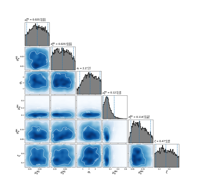
Figure 2: Posterior distribution for the spin model described in Sec. 2.2, assuming the Truncated Power Law BH mass function model and Double Gaussian NS mass distribution model. The contours represent 50% and 90% credible bounds, respectively.

4 simulation

We expect to have dozens of BNS/NSBH detections by the end of the fourth observing run of LIGO/Virgo/KAGRA network, and the number of events may reach one hundred within the duration of their fifth observing run (Abbott et al., 2018). Thus it is interesting to investigate whether we can determine the mass distribution of the NS via GWs in the next few years. In this section, we perform our analysis on mock GW detections generated from a prespecified underlying population. We assume the underlying NS mass distribution as that of the Galactic distribution, i.e., the Double Gaussian model (see Eq. (1)) with $m_{\rm min}=1M_{\odot}$, $m_{\rm max}=2.25$, $\mu_{1}=1.36M_{\odot}$, $\sigma_{1}=0.09M_{\odot}$, $\mu_{2}=1.9M_{\odot}$, $\sigma_{2}=0.5M_{\odot}$, and $r=0.65$. The BH mass distribution is described by the Truncated Power Law model (see Eq. (4)) with $m_{\rm low}=5M_{\odot}$, $m_{\rm up}=10M{\odot}$, and $\alpha=3$. The underlying spin distribution of binaries is described by Eq. (6), Eq. (7), and Eq. (8), with $\zeta=0.8$, $\sigma_{\rm t}=0.2$, $\mu_{\rm a}^{\rm BH}=0.1$, $\sigma_{\rm a}^{\rm BH}=0.1$, $\mu_{\rm a}^{\rm NS}=0.005$, and $\sigma_{\rm a}^{\rm NS}=0.01$. Additionally, the fraction of BNSs in the surveyed population (including both BNSs and NSBHs) is assumed to 0.7. In generating mock detections, we assume that the underlying population follows a uniform in comoving volume and source frame time merger rate, with isotropic sky positions and inclinations. The true values of ($m_{1}$, $m_{2}$, $a_{1}$, $a_{2}$, $z_{1}$, $z_{2}$) are drawn from the given distribution as described above. Additionally, $\phi_{\rm 12}$ and $\phi_{\rm jl}$ (i.e., azimuthal angle between the spins of the two components, azimuthal angle between the total binary angular momentum and the orbital angular momentum) are set to be uniform in (0, $2\pi$). The IMRPhenomXPHM waveform (London et al., 2018; Chatziioannou et al., 2017; Khan et al., 2019; García-Quirós et al., 2021) is used for generating simulated signals, and the identification of a GW signal is based on a network signal-to-noise ratio threshold $\rho_{th}=12$ and the design sensitivity noise curves (Abbott et al., 2018).

To obtain the posteriors for each ‘detected’ event, we apply the user-friendly software Bilby (Ashton et al., 2019) with sampler Pymultinest (Buchner, 2016) for parameter estimation. The sampling priors for single event parameter estimation are set as following: detector frame component masses are uniform in $(0.9,30)M_{\odot}$, spin magnitudes are uniform in (0, 1)/(0, 0.05) for BHs/NSs, the spin orientations are isotropic, the priors of distance and inclination angle are set assuming the binaries are uniform in comoving volume, source frame time, and with isotropic directions. In order to accelerate the inference, we fix the other extrinsic parameters (i.e., the sky coordinate, the polarization angle, the coalescing phase, and the coalescing time) as their injected values.

We find with 100 ‘detected’ events generated from the simulated population, we can rule out the Uniform distribution for NS mass by $\ln{\mathcal{B}}\sim 39$ (compared with the Double Gaussian model), and the Double gaussian model is more favored than the Single Gaussian model by $\ln{\mathcal{B}}\sim 19$ . The posteriors of hyperparameters for the Double Gaussian model are presented in Fig. 3, it is clear that the first peak of the NS mass distribution is well determined, while the second peak is ambiguous. The minimum and maximum masses of NS are both well constrained, additionally, the BNS fraction is constrained within uncertainty of 0.13 at 90% credible level. The distributions of NS mass modeled by the Double Gaussian and the Single Gaussian are shown in Fig. 4 (left). We can see that for the Double Gaussian model, the first peak is fairly significant, while the second peak is not obvious and it looks like a tail of the first peak. As for the Single Gaussian model, it fails to figure out the features of the injected population as is indicated by the Bayes factor mentioned above. The BH mass distribution is reconstructed by the Truncated Power Law, and all the hyperparameters are constrained well as presented in Fig. 4 (right). However, the spin properties of binaries are not well constrained, where $\mu^{\rm NS}_{a}=0.02^{+0.003}_{-0.004}$, $\sigma^{\rm NS}_{a}=0.004^{+0.003}_{-0.002}$, $\mu^{\rm BH}_{a}=0.168^{+0.019}_{-0.022}$, $\sigma^{\rm BH}_{a}=0.071^{+0.024}_{-0.016}$, $\sigma_{t}=0.87^{+0.20}_{-0.14}$, and $\zeta=0.93^{+0.06}_{-0.19}$.

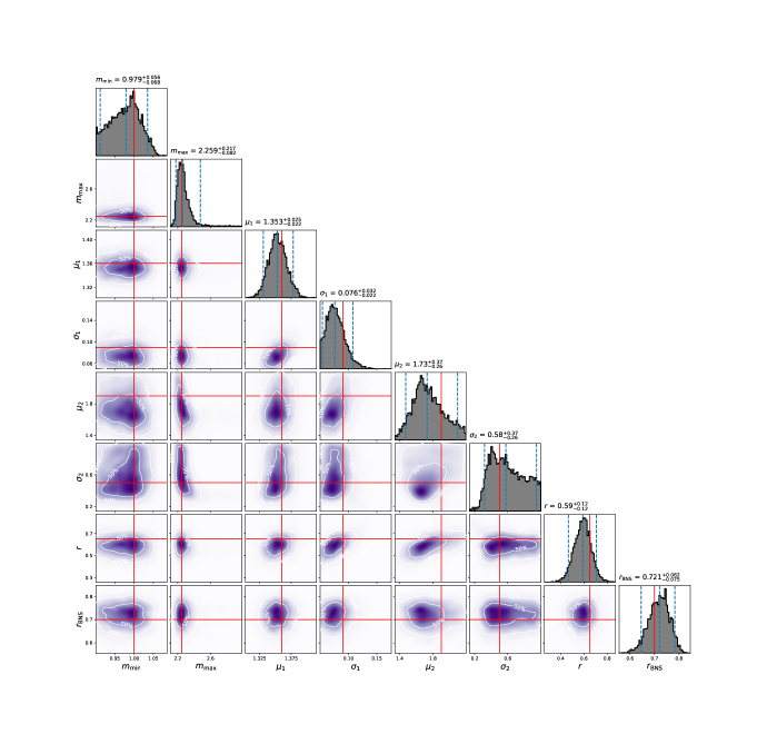
Figure 3: Posterior distribution for the NS mass hyperparameters inferred from 100 mock events. The contours represent 50% and 90% credible bounds, respectively, and the solid lines stand for the injected hyperparameters.

Figure 4: Left: Mass distributions of NSs inferred from the mock GW data with the Double Gaussian and Single Gaussian models. The black curves are the mass distribution of the injected population, and the shaded region represents the 90% credible interval. Right: Posterior distribution for the BH hyperparameter parameters inferred from the mock GW data. The contours represent 50% and 90% credible bounds, respectively, and the solid lines stand for the injected hyperparameter values.

5 Conclusion and Discussion

We perform hierarchical population inferences for the GW binaries involving at least one NS, and construct several synthesis models that include both the component masses and spin properties of the BNS and NSBH binaries, since there is a correlation between the component masses and the spin properties of compact binaries (Baird et al., 2013; Pratten et al., 2020; Abbott et al., 2021a). We have also performed inferences without spin information for comparison, and find that the corresponding evidence is slightly smaller than the inferences with spin information, e.g., $\ln{\mathcal{B}}=\ln{Z}_{\rm with~{}spin}-\ln{Z}_{\rm no~{}spin}=0.5$ for Double Gaussian NS mass distribution model + Truncated Power Law BH mass distribution model . The results are similar to those reported in Table 2, but the peak of Double Gaussian model in the spin-uninformative case is not as significant as that in the spin-informative case. Therefore, it is worthwhile to take the spin information into consideration when inferring the mass distribution of the compact binaries, though we do not aim to determine the spin properties of these kinds of binaries by currently limited observations.

Our main conclusion is that the three NS mass distribution models (i.e., Double Gaussian, Single Gaussian, and Uniform) can not be reliably distinguished by the current GW data. Our result is similar to Landry & Read (2021), where it is found that the Flat (in this work we call the Uniform) and Bimodal (i.e., the Double Gaussian in this work) models are equally preferred using the Akaike information criterion (Akaike, 1981). Nevertheless, there is a significant peak in the mass distribution obtained in our Double Gaussian model, and the location of the peak resembles that of Galactic NSs (Shao et al., 2020a). We further find that the mass distribution of Galactic NSs (Shao et al., 2020a) is slightly more preferred than the other models (by $\ln\mathcal{B}\sim 1.9$), which indicates that the NSs observed via GW signals may have the similar mass distribution as the NSs identified by electromagnetic observation in the Galaxy. This conclusion is different from Landry & Read (2021), where the authors find that the mass distribution of the NSs observed via GWs is unimodal, predicting far fewer low-mass and moderately more high-mass NSs in the population. This difference may be caused by the inclusion of the spin information of compact binaries into our hierarchical population inference. Another reason is that Landry & Read (2021) use a uniform distribution for BH masses with a pairing function $p(q)\propto q^{\beta_{q}}$ for NSBHs, while we use the models for BH masses as indicated by Özel et al. (2010).

Both the BH mass distribution models indicate a narrow distribution located in $\sim 5-10M_{\odot}$, which is consistent with the BHs in the Galactic X-ray binaries (Özel et al., 2010). As for the population of the compact binaries involving at least one NS, a fraction of $\sim 70\%$ is BNSs, and this result agrees with the merger rate densities of BNS and NSBH estimated by Abbott et al. (2021b) and Abbott et al. (2021a). Due to the currently limited sample and the measurement uncertainties of NS spins, the distribution of NS spin magnitudes is not well constrained. From the inferred result of spin orientations, we conclude that a perfectly aligned spin distribution can be ruled out, but a purely isotropic distribution of spin orientation is still allowed by the GW data.

Encouragingly, LIGO/Virgo/KAGRA will start their O4 and O5 observing runs in the next few years, at that time the sensitivities of GW detectors will be significantly improved (Abbott et al., 2018), and the detection number of such binaries like NSBHs and BNSs will exceed one dozen in the duration of O4 and may reach one hundred by the end of O5. By performing simulations, we find that the mass distribution of NS can be well determined with a total number of 100 events (including NSBHs and BNSs) via GW observations. We do not characterize the mass ratios of the binaries in our models currently, which may be a potential improvement in determining population properties of NSs. For instance, very recently, Tang et al. (2021b) find that there is a mild evidence for a mass correlation among the two components of the low mass ratio binaries. Therefore, if such a feature exists, the population properties of NSs in the coalescing compact binaries can be characterized more accurately. With the observation of NSs in binary systems via GW, we can study the properties of NSs in their final moments, while the radio pulsar observations of Galactic NSs enable us to study the properties of NSs in their midlife. Combining measurements from GW and radio, provides us with a more complete understanding of compact binaries (involving at least one NS) from formation to merger (Galaudage et al., 2021a). Additionally, the population difference between the extragalactic NSs and the galactic NSs may have an impact on the determination of the origin of the heavy elements (Wang et al., 2017; Chen et al., 2021). What’s more, the reliable measurement of NS mass distribution, enables us to better understand the equation of state of dense matter (Chatziioannou & Farr, 2020; Wysocki et al., 2020).

References

- Abbott et al. (2016) Abbott, B. P., Abbott, R., Abbott, T. D., et al. 2016, Phys. Rev. Lett., 116, 061102, doi: 10.1103/PhysRevLett.116.061102
- Abbott et al. (2017) —. 2017, Phys. Rev. Lett., 119, 161101, doi: 10.1103/PhysRevLett.119.161101
- Abbott et al. (2018) —. 2018, Living Reviews in Relativity, 21, 3, doi: 10.1007/s41114-018-0012-9
- Abbott et al. (2019a) —. 2019a, ApJ, 882, L24, doi: 10.3847/2041-8213/ab3800
- Abbott et al. (2019b) —. 2019b, Physical Review X, 9, 031040, doi: 10.1103/PhysRevX.9.031040
- Abbott et al. (2020a) —. 2020a, ApJ, 892, L3, doi: 10.3847/2041-8213/ab75f5
- Abbott et al. (2020b) Abbott, R., Abbott, T. D., Abraham, S., et al. 2020b, ApJ, 896, L44, doi: 10.3847/2041-8213/ab960f
- Abbott et al. (2020c) —. 2020c, Phys. Rev. Lett., 125, 101102, doi: 10.1103/PhysRevLett.125.101102
- Abbott et al. (2021a) —. 2021a, ApJ, 915, L5, doi: 10.3847/2041-8213/ac082e
- Abbott et al. (2021b) —. 2021b, Physical Review X, 11, 021053, doi: 10.1103/PhysRevX.11.021053
- Abbott et al. (2021c) —. 2021c, ApJ, 913, L7, doi: 10.3847/2041-8213/abe949
- Akaike (1981) Akaike, H. 1981, Journal of Econometrics, 16, 3, doi: https://doi.org/10.1016/0304-4076(81)90071-3
- Alsing et al. (2018) Alsing, J., Silva, H. O., & Berti, E. 2018, MNRAS, 478, 1377, doi: 10.1093/mnras/sty1065
- Antoniadis et al. (2016) Antoniadis, J., Tauris, T. M., Ozel, F., et al. 2016, arXiv e-prints, arXiv:1605.01665. https://arxiv.org/abs/1605.01665
- Ashton et al. (2019) Ashton, G., Hübner, M., Lasky, P. D., et al. 2019, Bilby: Bayesian inference library. http://ascl.net/1901.011
- Baird et al. (2013) Baird, E., Fairhurst, S., Hannam, M., & Murphy, P. 2013, Phys. Rev. D, 87, 024035, doi: 10.1103/PhysRevD.87.024035
- Baxter et al. (2021) Baxter, E. J., Croon, D., McDermott, S. D., & Sakstein, J. 2021, ApJ, 916, L16, doi: 10.3847/2041-8213/ac11fc
- Biswas et al. (2021) Biswas, B., Nandi, R., Char, P., Bose, S., & Stergioulas, N. 2021, MNRAS, 505, 1600, doi: 10.1093/mnras/stab1383
- Biwer et al. (2019) Biwer, C. M., Capano, C. D., De, S., et al. 2019, PASP, 131, 024503, doi: 10.1088/1538-3873/aaef0b
- Buchner (2016) Buchner, J. 2016, PyMultiNest: Python interface for MultiNest. http://ascl.net/1606.005
- Chatziioannou & Farr (2020) Chatziioannou, K., & Farr, W. M. 2020, Phys. Rev. D, 102, 064063, doi: 10.1103/PhysRevD.102.064063
- Chatziioannou et al. (2017) Chatziioannou, K., Klein, A., Yunes, N., & Cornish, N. 2017, Phys. Rev. D, 95, 104004, doi: 10.1103/PhysRevD.95.104004
- Chen et al. (2021) Chen, H.-Y., Vitale, S., & Foucart, F. 2021, arXiv e-prints, arXiv:2107.02714. https://arxiv.org/abs/2107.02714
- Creswell et al. (2018) Creswell, J., Liu, H., Jackson, A. D., von Hausegger, S., & Naselsky, P. 2018, J. Cosmology Astropart. Phys, 2018, 007, doi: 10.1088/1475-7516/2018/03/007
- Fan et al. (2020) Fan, Y.-Z., Jiang, J.-L., Tang, S.-P., Jin, Z.-P., & Wei, D.-M. 2020, ApJ, 904, 119, doi: 10.3847/1538-4357/abbf4e
- Farr & Chatziioannou (2020) Farr, W. M., & Chatziioannou, K. 2020, Research Notes of the American Astronomical Society, 4, 65, doi: 10.3847/2515-5172/ab9088
- Farrow et al. (2019) Farrow, N., Zhu, X.-J., & Thrane, E. 2019, ApJ, 876, 18, doi: 10.3847/1538-4357/ab12e3
- Fattoyev et al. (2020) Fattoyev, F. J., Horowitz, C. J., Piekarewicz, J., & Reed, B. 2020, Phys. Rev. C, 102, 065805, doi: 10.1103/PhysRevC.102.065805
- Fishbach & Holz (2020) Fishbach, M., & Holz, D. E. 2020, ApJ, 891, L27, doi: 10.3847/2041-8213/ab7247
- Galaudage et al. (2021a) Galaudage, S., Adamcewicz, C., Zhu, X.-J., Stevenson, S., & Thrane, E. 2021a, ApJ, 909, L19, doi: 10.3847/2041-8213/abe7f6
- Galaudage et al. (2021b) Galaudage, S., Talbot, C., Nagar, T., et al. 2021b, arXiv e-prints, arXiv:2109.02424. https://arxiv.org/abs/2109.02424
- García-Quirós et al. (2021) García-Quirós, C., Husa, S., Mateu-Lucena, M., & Borchers, A. 2021, Classical and Quantum Gravity, 38, 015006, doi: 10.1088/1361-6382/abc36e
- Gerosa et al. (2018) Gerosa, D., Berti, E., O’Shaughnessy, R., et al. 2018, Phys. Rev. D, 98, 084036, doi: 10.1103/PhysRevD.98.084036
- Han et al. (2020) Han, M.-Z., Tang, S.-P., Hu, Y.-M., et al. 2020, ApJ, 891, L5, doi: 10.3847/2041-8213/ab745a
- Jin et al. (2015) Jin, Z.-P., Li, X., Cano, Z., et al. 2015, ApJ, 811, L22, doi: 10.1088/2041-8205/811/2/L22
- Kalogera (2000) Kalogera, V. 2000, ApJ, 541, 319, doi: 10.1086/309400
- Khan et al. (2019) Khan, S., Chatziioannou, K., Hannam, M., & Ohme, F. 2019, Phys. Rev. D, 100, 024059, doi: 10.1103/PhysRevD.100.024059
- Kimball et al. (2020) Kimball, C., Talbot, C., Berry, C. P. L., et al. 2020, ApJ, 900, 177, doi: 10.3847/1538-4357/aba518
- Kimball et al. (2021) —. 2021, ApJ, 915, L35, doi: 10.3847/2041-8213/ac0aef
- Landry & Read (2021) Landry, P., & Read, J. S. 2021, arXiv e-prints, arXiv:2107.04559. https://arxiv.org/abs/2107.04559
- Li et al. (2017) Li, X., Hu, Y.-M., Jin, Z.-P., Fan, Y.-Z., & Wei, D.-M. 2017, ApJ, 844, L22, doi: 10.3847/2041-8213/aa7fb2
- Li et al. (2020) Li, Y.-J., Han, M.-Z., Tang, S.-P., et al. 2020, arXiv e-prints, arXiv:2012.04978. https://arxiv.org/abs/2012.04978
- Li et al. (2021) Li, Y.-J., Wang, Y.-Z., Han, M.-Z., et al. 2021, The Astrophysical Journal, 917, 33, doi: 10.3847/1538-4357/ac0971
- London et al. (2018) London, L., Khan, S., Fauchon-Jones, E., et al. 2018, Phys. Rev. Lett., 120, 161102, doi: 10.1103/PhysRevLett.120.161102
- Mapelli et al. (2021) Mapelli, M., Bouffanais, Y., Santoliquido, F., Arca Sedda, M., & Artale, M. C. 2021, arXiv e-prints, arXiv:2109.06222. https://arxiv.org/abs/2109.06222
- Nathanail et al. (2021) Nathanail, A., Most, E. R., & Rezzolla, L. 2021, ApJ, 908, L28, doi: 10.3847/2041-8213/abdfc6
- Nitz et al. (2021) Nitz, A., Harry, I., Brown, D., et al. 2021, gwastro/pycbc:, v1.16.14, Zenodo, doi: 10.5281/zenodo.5347736. https://doi.org/10.5281/zenodo.5347736
- Özel & Freire (2016) Özel, F., & Freire, P. 2016, ARA&A, 54, 401, doi: 10.1146/annurev-astro-081915-023322
- Özel et al. (2010) Özel, F., Psaltis, D., Narayan, R., & McClintock, J. E. 2010, ApJ, 725, 1918, doi: 10.1088/0004-637X/725/2/1918
- Pratten et al. (2020) Pratten, G., Schmidt, P., Buscicchio, R., & Thomas, L. M. 2020, Physical Review Research, 2, 043096, doi: 10.1103/PhysRevResearch.2.043096
- Qin et al. (2018) Qin, Y., Fragos, T., Meynet, G., et al. 2018, A&A, 616, A28, doi: 10.1051/0004-6361/201832839
- Qin et al. (2019) Qin, Y., Marchant, P., Fragos, T., Meynet, G., & Kalogera, V. 2019, ApJ, 870, L18, doi: 10.3847/2041-8213/aaf97b
- Rezzolla et al. (2018) Rezzolla, L., Most, E. R., & Weih, L. R. 2018, ApJ, 852, L25, doi: 10.3847/2041-8213/aaa401
- Rocha et al. (2019) Rocha, L. S., Bernardo, A., Horvath, J. E., Valentim, R., & de Avellar, M. G. B. 2019, Astronomische Nachrichten, 340, 957, doi: 10.1002/asna.201913743
- Rodriguez et al. (2016) Rodriguez, C. L., Zevin, M., Pankow, C., Kalogera, V., & Rasio, F. A. 2016, ApJ, 832, L2, doi: 10.3847/2041-8205/832/1/L2
- Ruiz et al. (2018) Ruiz, M., Shapiro, S. L., & Tsokaros, A. 2018, Phys. Rev. D, 97, 021501, doi: 10.1103/PhysRevD.97.021501
- Safarzadeh & Wysocki (2021) Safarzadeh, M., & Wysocki, D. 2021, ApJ, 907, L24, doi: 10.3847/2041-8213/abd8c7
- Shao et al. (2020a) Shao, D.-S., Tang, S.-P., Jiang, J.-L., & Fan, Y.-Z. 2020a, Phys. Rev. D, 102, 063006, doi: 10.1103/PhysRevD.102.063006
- Shao et al. (2020b) Shao, D.-S., Tang, S.-P., Sheng, X., et al. 2020b, Phys. Rev. D, 101, 063029, doi: 10.1103/PhysRevD.101.063029
- Shibata et al. (2019) Shibata, M., Zhou, E., Kiuchi, K., & Fujibayashi, S. 2019, Phys. Rev. D, 100, 023015, doi: 10.1103/PhysRevD.100.023015
- Speagle (2020) Speagle, J. S. 2020, MNRAS, 493, 3132, doi: 10.1093/mnras/staa278
- Stovall et al. (2018) Stovall, K., Freire, P. C. C., Chatterjee, S., et al. 2018, ApJ, 854, L22, doi: 10.3847/2041-8213/aaad06
- Talbot & Thrane (2017) Talbot, C., & Thrane, E. 2017, Phys. Rev. D, 96, 023012, doi: 10.1103/PhysRevD.96.023012
- Tang et al. (2021a) Tang, S.-P., Jiang, J.-L., Han, M.-Z., Fan, Y.-Z., & Wei, D.-M. 2021a, Phys. Rev. D, 104, 063032, doi: 10.1103/PhysRevD.104.063032
- Tang et al. (2021b) Tang, S.-P., Li, Y.-J., Wang, Y.-Z., Fan, Y.-Z., & Wei, D.-M. 2021b, arXiv e-prints, arXiv:2107.08811. https://arxiv.org/abs/2107.08811
- Tang et al. (2020) Tang, S.-P., Wang, H., Wang, Y.-Z., et al. 2020, ApJ, 892, 56, doi: 10.3847/1538-4357/ab77bf
- The LIGO Scientific Collaboration et al. (2021) The LIGO Scientific Collaboration, the Virgo Collaboration, Abbott, R., et al. 2021, arXiv e-prints, arXiv:2108.01045. https://arxiv.org/abs/2108.01045
- Thrane & Talbot (2019) Thrane, E., & Talbot, C. 2019, PASA, 36, e010, doi: 10.1017/pasa.2019.2
- Tiwari (2018) Tiwari, V. 2018, Classical and Quantum Gravity, 35, 145009, doi: 10.1088/1361-6382/aac89d
- Tiwari & Fairhurst (2021) Tiwari, V., & Fairhurst, S. 2021, ApJ, 913, L19, doi: 10.3847/2041-8213/abfbe7
- Valentim et al. (2011) Valentim, R., Rangel, E., & Horvath, J. E. 2011, MNRAS, 414, 1427, doi: 10.1111/j.1365-2966.2011.18477.x
- Vitale et al. (2017) Vitale, S., Lynch, R., Sturani, R., & Graff, P. 2017, Classical and Quantum Gravity, 34, 03LT01, doi: 10.1088/1361-6382/aa552e
- Wang et al. (2017) Wang, H., Zhang, F.-W., Wang, Y.-Z., et al. 2017, ApJ, 851, L18, doi: 10.3847/2041-8213/aa9e08
- Wang et al. (2021a) Wang, Y.-Z., Fan, Y.-Z., Tang, S.-P., Qin, Y., & Wei, D.-M. 2021a, arXiv e-prints, arXiv:2110.10838. https://arxiv.org/abs/2110.10838
- Wang et al. (2021b) Wang, Y.-Z., Tang, S.-P., Liang, Y.-F., et al. 2021b, ApJ, 913, 42, doi: 10.3847/1538-4357/abf5df
- Wong et al. (2021) Wong, K. W. K., Breivik, K., Kremer, K., & Callister, T. 2021, Phys. Rev. D, 103, 083021, doi: 10.1103/PhysRevD.103.083021
- Wysocki et al. (2018) Wysocki, D., Gerosa, D., O’Shaughnessy, R., et al. 2018, Phys. Rev. D, 97, 043014, doi: 10.1103/PhysRevD.97.043014
- Wysocki et al. (2020) Wysocki, D., O’Shaughnessy, R., Wade, L., & Lange, J. 2020, arXiv e-prints, arXiv:2001.01747. https://arxiv.org/abs/2001.01747
- Yang et al. (2015) Yang, B., Jin, Z.-P., Li, X., et al. 2015, Nature Communications, 6, 7323, doi: 10.1038/ncomms8323
- Zevin et al. (2021) Zevin, M., Bavera, S. S., Berry, C. P. L., et al. 2021, ApJ, 910, 152, doi: 10.3847/1538-4357/abe40e
- Zhu et al. (2018) Zhu, X., Thrane, E., Osłowski, S., Levin, Y., & Lasky, P. D. 2018, Phys. Rev. D, 98, 043002, doi: 10.1103/PhysRevD.98.043002