Analyzing Item Popularity Bias of Music Recommender Systems: Are Different Genders Equally Affected?

Abstract.

Several studies have identified discrepancies between the popularity of items in user profiles and the corresponding recommendation lists. Such behavior, which concerns a variety of recommendation algorithms, is referred to as popularity bias. Existing work predominantly adopts simple statistical measures, such as the difference of mean or median popularity, to quantify popularity bias. Moreover, it does so irrespective of user characteristics other than the inclination to popular content. In this work, in contrast, we propose to investigate popularity differences (between the user profile and recommendation list) in terms of median, a variety of statistical moments, as well as similarity measures that consider the entire popularity distributions (Kullback-Leibler divergence and Kendall’s $\tau$ rank-order correlation). This results in a more detailed picture of the characteristics of popularity bias. Furthermore, we investigate whether such algorithmic popularity bias affects users of different genders in the same way. We focus on music recommendation and conduct experiments on the recently released standardized LFM-2b dataset, containing listening profiles of Last.fm users. We investigate the algorithmic popularity bias of seven common recommendation algorithms (five collaborative filtering and two baselines). Our experiments show that (1) the studied metrics provide novel insights into popularity bias in comparison with only using average differences, (2) algorithms less inclined towards popularity bias amplification do not necessarily perform worse in terms of utility (NDCG), (3) the majority of the investigated recommenders intensify the popularity bias of the female users.

1. Introduction

Popularity bias in recommender systems refers to a disparity of item popularities in the recommendation lists. Most commonly, this means that a disproportionally higher number of popular items than less popular ones are recommended (Ekstrand et al., 2018). The existence of such a popularity bias has been evidenced in different domains already, e.g., movies (Abdollahpouri et al., 2019b), music (Kowald et al., 2020), or product reviews (Abdollahpouri et al., 2017). Collaborative filtering recommenders are particularly prone to popularity biases because the data they are trained on already exhibit an imbalance towards popular items, i.e., more user–item interactions are available for popular items than less popular ones (Abdollahpouri et al., 2019a).

The distribution of item popularities in most domains, in particular in the music domain, which we target in this work, shows a long-tail characteristic (Celma, 2010). A recommendation algorithm introduces no further algorithmic bias when the distribution of popularity values of recommended items (tracks) exactly matches the distribution of popularity values of already consumed items (listening history) for each user.

We identify two shortcomings of existing studies of popularity bias: First, popularity bias is commonly quantified using simple statistical aggregation metrics, predominantly comparing arithmetic means computed on some count of the user–item interactions (Abdollahpouri et al., 2019b; Kowald et al., 2020). These are not robust against outliers often present in music listening data. Second, popularity bias is typically studied irrespective of user characteristics. Therefore, the extent to which users of different groups (e.g., age, gender, or cultural background) are affected remains unclear. We set out to approach these shortcomings in the music domain by posing the following research questions:

• RQ1: Which novel insights into popularity bias can be obtained by quantifying algorithmic popularity bias based on the median, a variety of statistical moments, and similarity measures between popularity distributions?

• RQ2: Do algorithmic popularity biases affect users of different genders in the same way?

We find that users of different genders are affected by algorithm-inflected bias differently, such that the majority of the models expose female users to more biased results. Also, algorithms less inclined towards popularity bias amplification do not necessarily perform worse in terms of utility (NDCG). Finally, the studied metrics provide novel insights into popularity bias in comparison with only using average differences.

2. Related Work

We focuse on popularity bias, a well-studied form of bias in recommender systems research. This form of bias refers to the underrepresentation of less popular items in the produced recommendations and can lead to a significantly worse recommendation quality for consumers of long tail or niche items (Kowald et al., 2020; Lex et al., 2020; Abdollahpouri et al., 2019b; Jannach et al., 2015). Abdollahpouri et al. (2019b) show that state-of-the-art movie recommendation algorithms suffer from popularity bias, and introduce the delta-GAP metric to quantify the level of underrepresentation. As shown in Kowald et al. (2020), in particular users interested in niche, unpopular items suffer from a worse recommendation quality. The authors use the delta-GAP metric in the domain of music recommendations, and find that the delta-GAP metric does not show a difference between “niche” and “mainstream” users. The reason for this could be that a group-based metric is not suitable for the complexity of music styles, as user groups can be quite diverse within themselves (Kowald et al., 2021). Zhu et al. (2020) address a related problem of item under-recommendation bias, expressing it with ranking-based statistical parity and ranking-based equal opportunity metrics. Boratto et al. (2021) propose metrics quantifying the degree to which a recommender equally treats items along the popularity tail.

In contrast to these works, we study differences between popularity distributions of consumed and recommended items for each user. We express them in terms of the median as well as several statistical moments and similarity measures. In addition, we combine research strands on popularity bias and gender bias by analyzing how female and male listeners are affected by popularity bias.

3. Measuring Popularity Bias

We introduce ways to express popularity bias as quantified dissimilarity between popularity distributions of recommended and consumed items for each user.

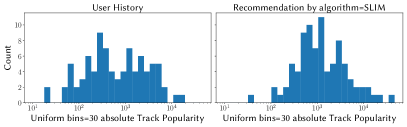
(a)

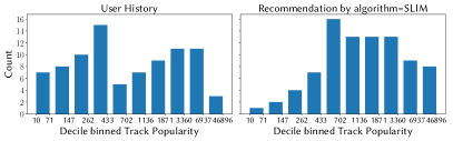
(b)

Figure 1. (a) shows equally binned (for visualization purposes only) distributions of popularity over the listening history (left) and the recommendation list (right) for the same user. On $x$-axis evenly binned popularity, on $y$-axis number of tracks in the distribution, falling into each bin. (b) demonstrates the same distributions binned with respect to the popularity distribution in the whole collection. This binning is employed for $KL$ and Kendall’s $\tau$ calculations.

3.1. Track Popularity Distributions

We define $P(t)$ popularity of a track $t$ as the sum of its play counts over all users $u_{i}\in U$ in the dataset, namely $P(t)=\sum_{u_{i}\in U}{PC(t,u_{i})}$. We then use these popularity estimates to derive the popularity distribution over each user’s listening history and recommendation list. In order to make the popularity distribution $H_{u_{i}}(t)$ over a user’s listening history $T_{hist}(u_{i})$ comparable to the respective distribution $R_{u_{i}}(t)$ over the recommendation lists, we consider only the top of the recommendation list $T_{top\_rec}(u_{i})$ so that its length (number of tracks) matches the length of the user’s listening history $|T_{top\_rec}(u_{i})|=|T_{hist}(u_{i})|$. Therefore, we define the popularity distribution over the listening history and the recommendation list of user $u_{i}$ as follows:

(1) $$H_{u_{i}}(t)=\begin{cases}P(t)|t\in T_{hist}(u_{i})\\ 0|t\notin T_{hist}(u_{i})\\ \end{cases} R_{u_{i}}(t)=\begin{cases}P(t)|t\in T_{top\_rec}(u_{i})\\ 0|t\notin T_{top\_rec}(u_{i})\\ \end{cases}$$

To gain a better understanding of these distributions, Figure 1(a) shows an example of popularity distributions over a user’s listening history $T_{hist}(u_{i})$ and the corresponding recommendation list $T_{top\_rec}(u_{i})$ produced by the SLIM recommender algorithm.

3.2. Metrics

3.2.1. Delta Metrics of Popularity Bias

In order to measure the differences between these distributions, we first introduce a series of delta metrics to calculate the discrepancies between the listening history and recommendation list popularity distributions of each user, and then aggregate them to achieve per-system results. We study five $\%\Delta\mathcal{M}$ (percent delta) metrics where the metric $\mathcal{M}$ is one of the following: $Mean$, $Median$, $Variance$, $Skew$, $Kurtosis$. If $\mathcal{M}(H_{u_{i}}(t))$ and $\mathcal{M}(R_{u_{i}}(t))$ are the results of application of the same metric $\mathcal{M}$ to the two respective distributions, the respective $\%\Delta\mathcal{M}$ for the user $u_{i}$ is calculated as: $\%\Delta\mathcal{M}_{u_{i}}=\frac{\mathcal{M}(R_{u_{i}}(t))-\mathcal{M}(H_{u_{i}}(t))}{\mathcal{M}(H_{u_{i}}(t))}\cdot 100$

Positive $\%\Delta Mean$ and $\%\Delta Median$ indicate that overall more popular tracks are recommended to the user. Since $Mean$ is sensitive to outliers, the interplay between these metrics provides additional information about the changes in popularity. Positive $\%\Delta Variance$ means that the list of recommended items is more diverse in terms of different popularity values than the user’s history. This can also mean an increase in bias towards more popular items, as the most popular items are sparsely distributed across the popularity range. Positive $\%\Delta Skew$ denotes that the right tail of the recommendation list distribution is heavier (with respect to the left tails) than the one belonging to the user-history distribution. A positive value therefore means that more items tend to have lower popularity from the range of the distribution. Finally, positive $\%\Delta Kurtosis$ shows that the tails of the recommended tracks’ popularity distribution are heavier than of its counterpart, and the distribution itself is in a way closer to uniform distribution.

Finally, the discussed metrics describe the difference between the distributions for a particular user. In order to represent the change across all users, we take the median of the per-user values.

3.2.2. Kullback–Leibler Divergence and Kendall’s $\tau$ as Measures for Popularity Bias

In order to compare the entire popularity distributions, we utilize Kullback–Leibler Divergence ($KL$) and Kendall’s $\tau$ ($KT$). For each user, we apply these metrics to the corresponding $H_{u_{i}}(t)$ and $R_{u_{i}}(t)$ decile-binned with respect to the popularity distribution over the whole collection ($P(t)$). The bins are chosen in such a way that the cumulative popularity of all tracks of the collection belonging into one bin constitutes approximately $10\%$ of the total popularity of all tracks of the whole collection. Figure 1(b) shows the distributions from Figure 1(a) binned this way. In our dataset, the bin corresponding to the most popular tracks is constituted by only $161$ items whose popularity ranges from about 7k to 47k total play counts. Each bin covers items that are roughly half as popular as the next decile bin and two times as popular as the previous decile bin. Such binning allows the two metrics to be less sensitive to minor differences between the distributions and concentrate on the shifts between different popularity categories.

$KL$ estimates the dissimilarity of two distributions, in our case, between the user’s listening history and recommendation list popularity distributions. It is defined as

(2) $$KL_{u_{i}}(\hat{H}_{u_{i}}(b)|\hat{R}_{u_{i}}(b))=\sum_{b_{j}\in B}{\hat{H}_{u_{i}}(b_{j})\log{\frac{\hat{H}_{u_{i}}(b_{j})}{\hat{R}_{u_{i}}(b_{j})}}}\vspace{-0.2cm}$$

where $\hat{H}_{u_{i}}(b)$ and $\hat{R}_{u_{i}}(b)$ are decile-binned and normalized versions of the distributions and $b_{j}\in B$ represent the ten bins. $KL$ compares the two distributions and increases with every mismatch in the item counts. It is particularly sensitive to the case when for a bin the user gets recommended fewer tracks than they have in their listening history.

While $KL$ Divergence is sensitive to actual count changes, Kendall’s $\tau$ metric reflects whether the order of bins is the same for the two distributions when ranked according to the respective counts. Kendall’s $\tau$ is calculated as $KT_{u_{i}}(\hat{H}_{u_{i}}(b),\hat{R}_{u_{i}}(b))=\frac{C-D}{C+D}$, where $C$ represents the number of pairs of bins that have the same respective ranking in both distributions (concordant pairs) and $D$ the number of pairs of bins that have the different respective ranking in the two distribution (discordant pairs). For example, looking at Figure 1(b), the first two bins are concordant ($\in C$) as in both cases, more items fall into the second bin. While the first and the last bins are discordant ($\in D$) as in the listening history distribution, the first bin has more items. However, the recommended distribution shows the opposite. This way, $KT$ shows whether there are common patterns (correlations) in the two distributions, and it reaches its maximum value of $1$ when the two distributions are identical from the bin-ranking point of view. Similar to $\%\Delta\mathcal{M}$ metrics, we use the median of the per-user values to measure the differences across all users for $KL$ and $KT$.

Table 1. Statistics of the dataset. Number of Users, Tracks and listening events (LEs) are reported across F(emale) and M(ale) separately and also together (All). Mean and standard deviation (indicated after $\pm$) of the interactions of users with tracks and LEs are indicated in the last three columns, respectively.

Gender	Users	Tracks	LEs	Tracks/User	LEs/User
All	$19,972$	$99,831$	$19,906,272$	$142\pm 172$	$997\pm 1,571$
F	$4,415$	$70,980$	$3,397,310$	$101\pm 121$	$769\pm 1,158$
M	$15,557$	$99,810$	$16,508,962$	$153\pm 182$	$1,061\pm 1,664$

4. Experiment Setup

4.1. Recommendation Algorithms

To study algorithmic popularity biases, we examine different commonly used collaborative filtering algorithms (i.e., heuristic, neighborhood based, matrix factorization, and autoencoders) (Dacrema et al., 2019; Melchiorre et al., 2021):

• Random Item (RAND): A baseline algorithm that recommends for each user random items. It avoids recommending already consumed items.

• Most Popular Items (POP): A baseline that implements a heuristic-based algorithm that recommends the same set of overall most popular items to each user.

• Item k-Nearest Neighbors (ItemKNN) (Deshpande and Karypis, 2004): A neighborhood-based algorithm that recommends items based on item-to-item similarity. Specifically, an item is recommended to a user if the item is similar to the items previously selected by the user. ItemKNN uses statistical measures to compute the item-to-item similarities.

• Sparse Linear Method (SLIM) (Ning and Karypis, 2011): Also a neighborhood-based algorithm, but instead of using predefined similarity metrics, the item-to-item similarity is learned directly from the data with a regression model.

• Alternating Least Squares (ALS) (Hu et al., 2008): A matrix factorization approach that learns user and item embeddings such that the dot product of these two approximates the original user-item interaction matrix.

• Matrix factorization with Bayesian Personalized Ranking (BPR) (Rendle et al., 2012): Learns user and item embeddings, however, with an optimization function that aims to rank the items consumed by the users according to their preferences (hence, personalized ranking) instead of predicting the rating for a specific pair of user and item.

• Variational Autoencoder (VAE) (Liang et al., 2018): An autoencoder-based algorithm that, given the user’s interaction vector, estimates a probability distribution over all the items using a variational autoencoder architecture.

For training the models, we use the same hyperparameter settings as provided by Melchiorre et al. (2021).

Table 2. Results of algorithm-inflected popularity bias evaluation in terms of the seven introduced metrics and NDCG@10. Each model is represented by three rows. The row $All$ gives the results on the whole dataset. The rows $\Delta Female$ and $\Delta Male$ describe the difference in the result between the user group and the whole population in the dataset. For example, the $\%\Delta Variance$ for algorithm SLIM for $All$ of $56.0$ denotes a median increase in popularity variance (between listening history and recommended list) of $56\%$ over all users. The corresponding $\Delta Female$ value of $-17.4$ means that the variance increase for this group is $56.0-17.4=38.6\%$.

Alg.	Users	$\%\Delta Mean$	$\%\Delta Median$	$\%\Delta Var.$	$\%\Delta Skew$	$\%\Delta Kurtosis$	$KL$	Kendall’s $\tau$	NDCG@10
	$All$	$-91.8$	$-87.2$	$-99.5$	$11.5$	$15.3$	$3.904$	$0.165$	$0.000$
2-10 RAND	$\Delta Female$	$-1.8$	$-3.5$	$-0.2$	$+0.0$	$-3.5$	$+0.976$	$-0.189$	$-0.000$
	$\Delta Male$	$+0.5$	$+1.1$	$+0.1$	$-0.0$	$+1.3$	$-0.281$	$+0.053$	$+0.000$
	$All$	$432.5$	$975.2$	$487.0$	$-58.0$	$-87.0$	$6.023$	$0.057$	$0.045$
2-10 POP	$\Delta Female$	$+11.0$	$+282.1$	$-172.2$	$-2.1$	$-1.9$	$+1.626$	$-0.033$	$+0.003$
	$\Delta Male$	$-2.8$	$-115.8$	$+55.9$	$+0.5$	$+0.5$	$-0.380$	$+0.016$	$-0.001$
	$All$	$121.8$	$316.6$	$72.6$	$-25.2$	$-43.9$	$4.368$	$0.046$	$0.184$
2-10 ALS	$\Delta Female$	$+9.9$	$+27.4$	$-7.1$	$-3.2$	$-5.4$	$+0.467$	$+0.110$	$-0.017$
	$\Delta Male$	$-2.7$	$-6.6$	$+1.6$	$+0.8$	$+1.5$	$-0.121$	$-0.023$	$+0.005$
	$All$	$-49.0$	$-3.7$	$-87.4$	$-14.8$	$-29.4$	$1.202$	$0.268$	$0.129$
2-10 BPR	$\Delta Female$	$+5.2$	$+7.7$	$+2.1$	$-1.4$	$-3.9$	$+0.476$	$-0.043$	$-0.011$
	$\Delta Male$	$-1.1$	$-1.9$	$-0.6$	$+0.4$	$+1.1$	$-0.110$	$+0.010$	$+0.003$
	$All$	$9.6$	$4.6$	$5.7$	$-14.3$	$-29.0$	$0.175$	$0.423$	$0.301$
2-10 ItemKNN	$\Delta Female$	$+2.0$	$+5.8$	$-2.6$	$-2.1$	$-3.2$	$+0.128$	$-0.037$	$-0.042$
	$\Delta Male$	$-0.5$	$-1.3$	$+0.9$	$+0.8$	$+0.9$	$-0.020$	$+0.008$	$+0.012$
	$All$	$49.8$	$99.8$	$56.0$	$-12.5$	$-26.0$	$0.424$	$0.189$	$0.365$
2-10 SLIM	$\Delta Female$	$-6.4$	$-13.1$	$-17.4$	$-1.7$	$-4.6$	$+0.217$	$+0.052$	$-0.048$
	$\Delta Male$	$+1.9$	$+3.9$	$+5.6$	$+0.6$	$+1.1$	$-0.029$	$-0.012$	$+0.014$
	$All$	$303.9$	$736.3$	$351.0$	$-45.2$	$-70.1$	$4.823$	$-0.028$	$0.191$
2-10 VAE	$\Delta Female$	$+10.1$	$+56.4$	$-69.3$	$-6.2$	$-6.6$	$+0.633$	$+0.146$	$-0.020$
	$\Delta Male$	$-2.3$	$-20.4$	$+17.3$	$+1.8$	$+2.1$	$-0.161$	$-0.042$	$+0.006$

4.2. Dataset and Evaluation Protocol

We perform experiments on LFM-2b-DemoBias (Melchiorre et al., 2021), a subset of the LFM-2b dataset. As in (Melchiorre et al., 2021), we only consider user-track interactions with a playcount (PC) ¿ 1, possibly avoiding using spurious interactions likely introduced by noise. Furthermore, we only consider tracks listened to by at least 5 different users and, likewise, only users who listened to at least 5 different tracks. Moreover, we only consider listening events within the last 5 years, letting us focus more on possible popularity biases in the recent years. Lastly, we consider binary user-track interactions, i.e., 1 if the user has listened to the track at least once, 0 otherwise.

The procedure described above results in a subset of 23k users over 1.6 million items. We finalize data preparation by sampling 100k tracks uniformly-at-random, which ensures that tracks of different popularity levels are equally likely to be included in the final dataset. The statistics of the final dataset are reported in Table 1. We find that males represent the majority group in the dataset and that they create $\sim 80\%$ of all listening events.

As evaluation protocol, we employ a user-based split strategy (Liang et al., 2018; Marlin, 2004), i.e., we split the 19,972 users in the dataset into train, validation, and test user groups via a 60-20-20 ratio split. We carry out 5-fold cross validation and change these user groups in a round-robin fashion. The users in the training set and all their interactions are used to train the recommendation algorithms. For testing and validation, we follow standard setups (Liang et al., 2018; Steck, 2019) and randomly sample 80% of the users’ items as input for the recommendation models and use the remaining 20% to calculate the evaluation metric.

5. Results and Discussion

The results are shown in Table 2. Each value in the All rows, regarding the popularity bias metrics, shows the median value of the distribution of a given metric over all users. For instance, $\%\Delta Var.$ of 72.6% for ALS denotes that the median increase in popularity variance is 72.6 percent between user’s listening history and items recommended to each user across all users. SLIM $KL$ 1.66 expresses that the median difference between user history popularity distributions and the corresponding recommended tracks popularity distributions is 1.66 in terms of $KL$ Divergence. The reported results regarding the genders indicate the changes in values in respect to the All values.

Both baseline algorithms (RAND and POP) show poor results on accuracy metrics. Notably, on the $\%\Delta$ popularity bias metrics, they show divergent behavior. Decreasing of $\%\Delta$ metrics of $Mean$, $Median$, $Variance$ and increasing of $Skew$ and $Kurtosis$ indicate that RAND provides a list of tracks whose popularity distribution is closer to uniform than those from users’ listening histories. POP has an opposite trend, as the recommended tracks’ popularity distribution has a more pronounced peak, is skewed, and shifted towards more popular items. It also shows a substantial median increase of variance in popularity, which can be explained by the fact that in our dataset, the most popular tracks are sparsely distributed across a wide range of popularity values ($161$ track in the popularity range between 7k and 47k of total play counts). Thus, recommending tracks from this category leads to a high variance. High values for $KL$ for both baselines also indicate that the overall popularity distributions of the recommended items are highly different from those of the users’ listening histories. The random recommender demonstrates a higher median Kendall’s $\tau$, which means that its output better correlates with users’ histories in terms of popularity distribution. Both neighborhood-based models (i.e., ItemKNN and SLIM) show a high performance in terms of NDCG and a moderate popularity bias in their recommendations according to the $\%\Delta$ metrics, which is lower compared to VAE and ALS. In particular, SLIM shows higher value in $\%\Delta$ $Mean$ and $Median$ compared to ItemKNN, suggesting that the item-to-item similarities learned by SLIM favors more popular items in the recommendations. ItemKNN displays lower $KL$ and higher Kendall’s $\tau$ than SLIM, which means that its results better approximate users’ listening histories (we attribute this to ItemKNN being less sensitive to bias in the data as it does not require trainable parameters). These observations regarding the performance of the models indicate that a decrease in popularity bias does not necessarily lead to a significant performance drop. Comparing ALS with BPR, we can observe an opposite behavior. While providing less biased results, BPR shows the poorest performance among all non-baseline algorithms. While VAE is similarly biased in terms of all metrics as POP, it achieves a higher performance according to NDCG.

Comparing metrics between the two gender groups, we note that $\%\Delta$ $Mean$ and $Median$ is higher for female users. That means that their recommendations contain more popular items and/or items of higher popularity than the ones they usually listen to, and for this user group, that effect is more pronounced (hence larger values). Considering that $\%\Delta Variance$ is lower for the female users, we conclude that their recommendations are less diverse in terms of track popularity while consisting of more popular items. Judging by $\%\Delta$ $Skew$, $Kurtosis$ as well as Kendall’s $\tau$, we can suggest that most recommender algorithms provide recommendations with comparable popularity distributions to both male and female users. At the same time, a slightly larger $KL$ may mean a larger shift towards popular items for female users. ItemKNN is the least biased algorithm in our study. It features low absolute values of $\%\Delta$ $Mean$, $Median$ and $Variance$, meaning that its recommendations consist of tracks comparable to the user’s listening history in terms of average popularity and variety. High Kendall’s $\tau$ means that the shape of the popularity distribution of the recommendations best matches the user’s history among all tested algorithms. Still, it is slightly biased towards more popular items, as shown by negative $\%\Delta$ $Skew$ and $KL$ (which combined with high Kendall’s $\tau$ signalizes about a shift of the distribution).

6. Conclusions and Future Direction

In this paper, we examine to what extent various music recommender systems amplify item popularity bias. We study seven metrics of popularity bias deviation and analyze the results of seven recommender algorithms for users of different genders and for the overall population in the dataset. Addressing RQ1, we observe that the studied metrics capture considerably different aspects of difference between popularity distributions of consumed and recommended items. While $\%\Delta Mean$ and $\%\Delta Median$ tell us about overall trends (are recommended tracks more or less popular than consumed ones), $\%\Delta Variance$ expresses the change in the diversity between listening histories and recommendation lists, and $\%\Delta Skew$ and $\%\Delta Kurtosis$ hint on the difference of shapes between the two distributions. Finally, $KL$ Divergence and Kendall’s $\tau$ allow insight into how well the distributions match on a more granular level. With regard to RQ2, we found that while the investigated algorithms display various levels of popularity bias, the majority of them (VAE, ItemKNN, BPR, ALS) expose the female users to more popularity biased results. In the future, we will approach mitigating model-imposed popularity bias, e.g., through adversarial training or incorporating bias into the loss function of the recommenders, as well as finding more expressive metrics describing differences in the popularity distributions. Additionally, we plan to split our users into groups according to mainstreaminess as in (Kowald et al., 2020) to compare our metrics with the group-based delta-GAP metric used in that work.

- (1)
- Abdollahpouri et al. (2017) Himan Abdollahpouri, Robin Burke, and Bamshad Mobasher. 2017. Controlling popularity bias in learning-to-rank recommendation. In Proceedings of the eleventh ACM conference on recommender systems. 42–46.
- Abdollahpouri et al. (2019a) Himan Abdollahpouri, Robin Burke, and Bamshad Mobasher. 2019a. Managing popularity bias in recommender systems with personalized re-ranking. In The thirty-second international flairs conference.
- Abdollahpouri et al. (2019b) Himan Abdollahpouri, Masoud Mansoury, Robin Burke, and Bamshad Mobasher. 2019b. The Unfairness of Popularity Bias in Recommendation. In Proceedings of the Workshop on Recommendation in Multi-stakeholder Environments co-located with the 13th ACM Conference on Recommender Systems (RecSys 2019), Copenhagen, Denmark, September 20, 2019 (CEUR Workshop Proceedings, Vol. 2440). CEUR-WS.org. http://ceur-ws.org/Vol-2440/paper4.pdf
- Boratto et al. (2021) Ludovico Boratto, Gianni Fenu, and Mirko Marras. 2021. Connecting user and item perspectives in popularity debiasing for collaborative recommendation. Information Processing & Management 58, 1 (Jan 2021), 102387. https://doi.org/10.1016/j.ipm.2020.102387
- Celma (2010) Òscar Celma. 2010. Music Recommendation and Discovery - The Long Tail, Long Fail, and Long Play in the Digital Music Space. Springer. https://doi.org/10.1007/978-3-642-13287-2
- Dacrema et al. (2019) Maurizio Ferrari Dacrema, Paolo Cremonesi, and Dietmar Jannach. 2019. Are we really making much progress? A worrying analysis of recent neural recommendation approaches. In Proceedings of the 13th ACM Conference on Recommender Systems. 101–109.
- Deshpande and Karypis (2004) Mukund Deshpande and George Karypis. 2004. Item-based top-n recommendation algorithms. ACM Transactions on Information Systems (TOIS) 22, 1 (2004), 143–177.
- Ekstrand et al. (2018) Michael D Ekstrand, Mucun Tian, Ion Madrazo Azpiazu, Jennifer D Ekstrand, Oghenemaro Anuyah, David McNeill, and Maria Soledad Pera. 2018. All the cool kids, how do they fit in?: Popularity and demographic biases in recommender evaluation and effectiveness. In Conference on Fairness, Accountability and Transparency. 172–186.
- Hu et al. (2008) Yifan Hu, Yehuda Koren, and Chris Volinsky. 2008. Collaborative filtering for implicit feedback datasets. In 2008 Eighth IEEE International Conference on Data Mining. Ieee, 263–272.
- Jannach et al. (2015) Dietmar Jannach, Lukas Lerche, and Iman Kamehkhosh. 2015. Beyond ”Hitting the Hits”: Generating Coherent Music Playlist Continuations with the Right Tracks. In Proceedings of the 9th ACM Conference on Recommender Systems (Vienna, Austria) (RecSys ’15). ACM, New York, NY, USA, 187–194. https://doi.org/10.1145/2792838.2800182
- Kowald et al. (2021) Dominik Kowald, Peter Muellner, Eva Zangerle, Christine Bauer, Markus Schedl, and Elisabeth Lex. 2021. Support the underground: characteristics of beyond-mainstream music listeners. EPJ Data Science 10, 1 (2021), 1–26.
- Kowald et al. (2020) Dominik Kowald, Markus Schedl, and Elisabeth Lex. 2020. The Unfairness of Popularity Bias in Music Recommendation: A Reproducibility Study. In Advances in Information Retrieval - 42nd European Conference on IR Research, ECIR 2020, Lisbon, Portugal, April 14-17, 2020, Proceedings, Part II (Lecture Notes in Computer Science, Vol. 12036). Springer, 35–42. https://doi.org/10.1007/978-3-030-45442-5_5
- Lex et al. (2020) Elisabeth Lex, Dominik Kowald, and Markus Schedl. 2020. Modeling popularity and temporal drift of music genre preferences. Transactions of the International Society for Music Information Retrieval 3, 1 (2020).
- Liang et al. (2018) Dawen Liang, Rahul G Krishnan, Matthew D Hoffman, and Tony Jebara. 2018. Variational autoencoders for collaborative filtering. In Proceedings of the 2018 world wide web conference. 689–698.
- Marlin (2004) Benjamin Marlin. 2004. Collaborative filtering: A machine learning perspective. University of Toronto Toronto.
- Melchiorre et al. (2021) Alessandro B. Melchiorre, Navid Rekabsaz, Emilia Parada-Cabaleiro, Stefan Brandl, Oleg Lesota, and Markus Schedl. 2021. Investigating gender fairness of recommendation algorithms in the music domain. Information Processing & Management 58, 5 (2021), 102666. https://doi.org/10.1016/j.ipm.2021.102666
- Ning and Karypis (2011) Xia Ning and George Karypis. 2011. Slim: Sparse linear methods for top-n recommender systems. In 2011 IEEE 11th International Conference on Data Mining. IEEE, 497–506.
- Rendle et al. (2012) Steffen Rendle, Christoph Freudenthaler, Zeno Gantner, and Lars Schmidt-Thieme. 2012. BPR: Bayesian personalized ranking from implicit feedback. arXiv preprint arXiv:1205.2618 (2012).
- Steck (2019) Harald Steck. 2019. Embarrassingly Shallow Autoencoders for Sparse Data. In The World Wide Web Conference, WWW 2019, San Francisco, CA, USA, May 13-17, 2019, Ling Liu, Ryen W. White, Amin Mantrach, Fabrizio Silvestri, Julian J. McAuley, Ricardo Baeza-Yates, and Leila Zia (Eds.). ACM, 3251–3257. https://doi.org/10.1145/3308558.3313710
- Zhu et al. (2020) Ziwei Zhu, Jianling Wang, and James Caverlee. 2020. Measuring and Mitigating Item Under-Recommendation Bias in Personalized Ranking Systems. Association for Computing Machinery, New York, NY, USA, 449–458. https://doi.org/10.1145/3397271.3401177