Uniform Function Estimators in Reproducing Kernel Hilbert Spaces

Abstract

This paper addresses the problem of regression to reconstruct functions, which are observed with superimposed errors at random locations. We address the problem in reproducing kernel Hilbert spaces. It is demonstrated that the estimator, which is often derived by employing Gaussian random fields, converges in the mean norm of the reproducing kernel Hilbert space to the conditional expectation and this implies local and uniform convergence of this function estimator. By preselecting the kernel, the problem does not suffer from the curse of dimensionality.

The paper analyzes the statistical properties of the estimator. We derive convergence properties and provide a conservative rate of convergence for increasing sample sizes.

Keywords: Reproducing kernel Hilbert spaces • positive definite functions • Gramian matrix • Mercer kernels • Statistical learning theory

Classification: 62G05, 62G08, 62G20

1 Introduction

This paper addresses the problem of regression and approximation, nowadays occasionally often associated with the term statistical learning. The specific estimator we consider is based on kernel functions. We investigate the estimator’s convergence properties in the the genuine and most natural norm, the norm induced by the kernel function itself.

The estimator is often derived by involving Gaussian random fields and is central in support vector machines as well, an additional motivational point to investigate its specific properties. Here, the estimator is often inferred with least squares errors and by involving a regularization term based on a reproducing kernel Hilbert space. The literature frequently employs loss and risk functionals, and involves an $L^{2}$-error to investigate this estimator. Our results complement these research directions by adding the natural, genuine norm. They enable us to establish uniform convergence of the estimator by moderately regularizing the objectives. This uniform convergence is indeed essential and crucial for applications in stochastic optimization.

Explicit convergence rates are presented for increasing sample sizes. The results and convergence rates correspond to other rates known from non-parametric statistics, particularly to density estimation when employing the mean (integrated) squared error. Starting with a fixed kernel, the results presented here do not depend on the dimension of the design space, so they do not suffer from what is occasionally addressed by the catchphrase curse of dimensionality.

Cucker and Zhou [5] provide an introduction to approximation theory in a random framework. The excellent book Bishop [3, Section 2.3] gives very concrete applications in statistical learning theory, while Wendland [22] provide the mathematical foundations for approximations in reproducing kernel Hilbert spaces. The monograph Steinwart and Christmann [20] introduces to support vector machines, which employ kernel functions similarly to our approach presented below. A study, comparably to ours but employing a simpler norm, is Zhang et al. [23]. Caponnetto and De Vito [4] provide the state of the art for an analysis in $L^{2}$ involving the kernel operator, see also Györfi et al. [7].

Outline of the paper.

The following Section 2 repeats elements from reproducing kernel Hilbert spaces, which are of importance throughout this paper. Section 3 introduces the elementary estimator, which is employed in statistical learning. Sample average approximation (Section 3.2) address this estimator with random samples from both dimensions and Section 5.15 reveals related statistical results. The Sections 5 and 6 derive our main results, which is, for short, convergence of the sample average optimizer in mean norm and weak consistency (Section 6.3) of this estimator. Section 7 concludes with a summary.

2 Regularization with reference to reproducing kernel Hilbert spaces

Throughout we shall expose the problem on the design space $\mathcal{X}$, an arbitrary set for which we require more structure later; most typically, $\mathcal{X}$ is a subset of $\mathbb{R}^{d}$. Let $(X_{i},f_{i})$, $i=1,\dots,n$, be independent, identically distributed observations in $\mathcal{X}\times\mathbb{R}$ with joint probability measure $\mathcal{\rho}$. For a kernel function $k\colon\mathcal{X}\times\mathcal{X}\to\mathbb{R}$ we consider the estimator

$$\hat{f}_{n}(\cdot)=\frac{1}{n}\sum_{i=1}^{n}k(\cdot,X_{i})\,\hat{w}_{i},$$ (2.1)

where the weights $\hat{w}_{i}$ satisfy the system of linear equations

$$\lambda_{n}\,\hat{w}_{i}+\frac{1}{n}\sum_{j=1}^{n}k(X_{i},X_{j})\,\hat{w}_{j}=f_{i},\qquad i=1,\dots,n,$$ (2.2)

for some parameter $\lambda_{n}$. In what follows we derive this estimator first by employing Gaussian random fields and kernel ridge regression from support vector machines and then investigate and expose its convergence properties. Specifically, we identify and characterize the function $f$ so that

$$\operatorname{{\mathds{E}}}\|\hat{f}_{n}(\cdot)-f(\cdot)\|^{2}\to 0$$ (2.3)

as $n\to\infty$, where $\|\cdot\|$ is a norm and $\lambda_{n}$ is chosen adequately; above all, we derive results for the norm of the reproducing kernel Hilbert space associated with the kernel function. We will also infer convergence results for $L^{2}$ and—most importantly—for uniform function approximations, as point evaluations are continuous in the kernel norm.

2.1 Gaussian random fields

As an initial motivation for the estimator (2.1) consider a zero mean Gaussian random field $f$ on $\mathcal{X}$ with covariance function $k\colon\mathcal{X}\times\mathcal{X}\to\mathbb{R}$, that is, $k(x,y)=\operatorname{cov}\big{(}f(x),f(y)\big{)}$. For a signal plus noise model with observations

$$f_{i}=f(x_{i})+\varepsilon_{i},$$

the joint distribution, including $x$ to the observation points $X=(x_{1},\dots,x_{n})$, is

$$\begin{pmatrix}f(x)\\ f\end{pmatrix}\sim\mathcal{N}\left(\begin{pmatrix}0\\ 0\end{pmatrix},\ \begin{pmatrix}k(x,x)&k(x,X)\\ k(X,x)&k(X,X)+\lambda\end{pmatrix}\right),$$

where $\varepsilon\sim\mathcal{N}(0,\lambda)$ is the independent error and where we use the compact vector notation $f\coloneqq(f_{1},\dots,f_{n})^{\top}$ and $k(x,X)\coloneqq\big{(}k(x,x_{1}),\dots,k(x,x_{n})\big{)}$ for the entry of the covariance matrix; the other entries are defined analogously. With this, the conditional distribution is

$$f(x)\mid\big{(}f(X)=f\big{)}\sim\mathcal{N}\big{(}\hat{\mu}(x),\,\hat{K}(x)\big{)},$$

where

$$\hat{\mu}(x)\coloneqq k(x,X)\big{(}k(X,X)+\lambda\big{)}^{-1}f(X)$$ (2.4)

is the mean and the variance is

$$\hat{K}(x)\coloneqq k(x,x)-k(x,X)\big{(}k(X,X)+\lambda\big{)}^{-1}k(X,x),$$ (2.5)

see Shiryaev [19, Theorem 13.1] or Bishop [3, Section 2.3]. Expanding (2.4) and setting $\hat{f}_{n}(x)\coloneqq\hat{\mu}(x)$ reveals the initial estimator (2.1) for variance $\lambda$ rescaled. Figure 1a displays an example of the estimator $\hat{f}_{n}(\cdot)$ together with the range $\pm\sqrt{\hat{K}(\cdot)}$ from (2.5).

2.2 Reproducing kernel Hilbert space

Every estimator $\hat{f}_{n}(\cdot)$ in (2.1) is an element in the reproducing kernel Hilbert space spanned by the functions $k(\cdot,y)$, $y\in\mathcal{X}$. While introducing the notation for reproducing kernel Hilbert spaces here we briefly recall major properties, which are essential in our following exposition. For a general discussion on reproducing kernel Hilbert spaces we may refer to Mandrekar and Gawarecki [11, Chapter 1].

Definition 2.1.

The kernel is a symmetric and positive definite function $k\colon\mathcal{X}\times\mathcal{X}\to\mathbb{R}$. On the linear span $\{k(\cdot,x)\colon\mathcal{X}\to\mathbb{R}\mid x\in\mathcal{X}\}$ of functions on $\mathcal{X}$, the inner product is defined by

$$\bigl{\langle}k(\cdot,x)\mid k(\cdot,y)\bigr{\rangle}_{k}\coloneqq k(x,y).$$ (2.6)

The reproducing kernel Hilbert space, denoted $\big{(}\mathcal{H}_{k},\|\cdot\|_{k}\big{)}$, is the completion with respect to the norm $\|f\|_{k}^{2}\coloneqq\left\langle f\mid f\right\rangle_{k}$ induced by the inner product (2.6).

Most importantly, point evaluations are continuous linear functions in reproducing kernel Hilbert spaces. Indeed, finite linear combinations $f(\cdot)=\sum_{i=1}^{n}k(\cdot,x_{i})\,w_{i}$ are dense in $\mathcal{H}_{k}$ and it follows from (2.6) that

$$\bigl{\langle}k(\cdot,x)\big{|}\,f\bigr{\rangle}_{k}=\sum_{i=1}^{n}w_{i}\,\bigl{\langle}k(\cdot,x)\big{|}\,k(\cdot,x_{i})\bigr{\rangle}_{k}=\sum_{i=1}^{n}w_{i}\,k(x,x_{i})=f(x).$$ (2.7)

Although more general settings are easily possible, in what follows we convene to address only continuous and uniformly bounded kernel functions $k$. We associate the following Hilbert–Schmidt integral operator $K$ with a kernel $k$.

Definition 2.2 (Design measure).

Let $\mathcal{X}$ be a measure space. The marginal measure $P(\cdot)\coloneqq\rho(\cdot\times\mathbb{R})$ is the design measure.

Definition 2.3.

Let $k$ be a kernel. The operator $K\colon L^{2}(\mathcal{X})\to L^{2}(\mathcal{X})$ is

$$K\,w(x)\coloneqq\int_{\mathcal{X}}k(x,y)\,w(y)\,P(dy),$$ (2.8)

where $w\in L^{2}(\mathcal{X})$.

Proposition.

The operator $K$ is self-adjoint and positive definite with respect to the standard inner product

$$\left\langle f\mid g\right\rangle\coloneqq\int_{\mathcal{X}}f(z)\cdot g(z)\,P(dz)$$

on $\big{(}L^{2},\|\cdot\|_{2}\big{)}$. The operator is positive definite and bounded with norm

$$\|K\colon L^{2}\to L^{2}\|^{2}\leq\iint_{\mathcal{X}^{2}}k(x,y)^{2}\,P(dx)P(dy).$$

Proof.

The assertion is a consequence of the Cauchy–Schwarz inequality. ∎

Proposition 2.4.

It holds that $\|k(\cdot,x)\|_{k}^{2}=k(x,x)$,

$$\left\langle Kw\mid f\right\rangle_{k}=\left\langle w\mid f\right\rangle\quad\text{and}\quad\left\|Kw\right\|_{k}^{2}=\left\langle w\mid Kw\right\rangle.$$ (2.9)

Proof.

The functions $f(\cdot)=\sum_{i=1}^{n}w_{i}^{\prime}\,k(\cdot,x_{i})$ are dense in $\mathcal{H}_{k}$. By linearity,

$$\left\langle Kw\mid f\right\rangle_{k} =\sum_{i=1}^{n}\,w_{i}^{\prime}\int_{\mathcal{X}}\big{<}k(\cdot,y)\mid k(\cdot,x_{i})\big{>}_{k}w(y)\,P(dy)$$

$$=\int_{\mathcal{X}}\sum_{i=1}^{n}\,w_{i}^{\prime}\,k(y,x_{i})\,w(y)\,P(dy)$$

$$=\int_{\mathcal{X}}f(y)\,w(y)\,P(dy)$$

$$=\left\langle w\mid f\right\rangle.$$

The other assertions are immediate. ∎

Remark 2.5 (Mercer and the kernel trick).

The operator $K$ is compact with $k(x,y)=\sum_{\ell=1}^{\infty}\sigma_{\ell}^{2}\,\phi_{\ell}(x)\,\phi_{\ell}(y)$, where $\sigma_{\ell}^{2}$ is the eigenvalue corresponding to the eigenfunction $\phi_{\ell}(\cdot)$. In this setting, the operator $K^{\nicefrac{{1}}{{2}}}$ is $K^{\nicefrac{{1}}{{2}}}f=\sum_{\ell=1}^{\infty}\sigma_{\ell}\,\phi_{\ell}\left\langle\phi_{\ell}\mid f\right\rangle$ (with $\sigma_{\ell}\geq 0$), see Reed and Simon [13, Theorem VI.23].

Proposition 2.6 ($K^{\nicefrac{{1}}{{2}}}\colon L^{2}\to\mathcal{H}_{k}$ is an isometry).

It holds that $\|K^{\nicefrac{{1}}{{2}}}f\|_{k}=\|f\|_{2}$ and $\|f\|_{2}\leq\|K\|^{\nicefrac{{1}}{{2}}}\cdot\|f\|_{k}$.

Proof.

The assertion is a consequence of Mercer’s theorem, cf. König [10] and Hein and Bousquet [8, Corollary 4]. However, for $f=K^{\nicefrac{{1}}{{2}}}w$ it follows from the preceding proposition that

$$\|K^{\nicefrac{{1}}{{2}}}f\|_{k}^{2}=\|Kw\|_{k}^{2}=\left\langle w\mid Kw\right\rangle=\left\langle K^{\nicefrac{{1}}{{2}}}w\mid K^{\nicefrac{{1}}{{2}}}w\right\rangle=\|f\|_{2}^{2}.$$

With (2.9) we have further that

$$\|f\|_{2}^{2}=\big{<}K^{\nicefrac{{1}}{{2}}}w\mid K^{\nicefrac{{1}}{{2}}}w\big{>}=\bigl{\langle}w\mid Kw\bigr{\rangle}\leq\|K\|\,\|w\|_{2}^{2}=\|K\|\,\|K^{\nicefrac{{1}}{{2}}}w\|_{k}^{2}=\|K\|\,\|f\|_{k}^{2},$$

as $K$ is self-adjoint. Hence the assertion. ∎

Theorem 2.7 (Continuity of the operator $K$).

It holds that $\|K\colon\mathcal{H}_{k}\to\mathcal{H}_{k}\|\leq\|K\colon L_{2}\to L_{2}\|$.

Proof.

With (2.9) and Proposition 2.6, $\|Kf\|_{k}^{2}=\left\langle f\mid Kf\right\rangle\leq\|K\|\,\|f\|_{2}^{2}\leq\|K\|^{2}\|f\|_{k}^{2}$ and hence the assertion. ∎

We have seen in (2.7) that point evaluations are linear functionals. We shall conclude here by relating these norms to uniform convergence.

Proposition 2.8.

The point evaluation is continuous; indeed, $|f(x)|\leq\sqrt{k(x,x)}\,\|f\|_{k}$ for all $x\in\mathcal{X}$ and $f\in\mathcal{H}_{k}$. Further,

$$\|f\|_{\infty}\leq\|f\|_{k}\cdot\sup_{x\in\operatorname{supp}P}\sqrt{k(x,x)},$$ (2.10)

where $\|f\|_{\infty}\coloneqq\sup_{x\in\operatorname{supp}P}|f(x)|$.

Proof.

The statement is immediate from (2.7), as

$$|f(x)|=\big{|}\big{<}k(\cdot,x)\big{|}\,f\big{>}_{k}\big{|}\leq\|k(\cdot,x)\|_{k}\,\|f\|_{k}=\sqrt{k(x,x)}\,\|f\|_{k}$$

by the Cauchy–Schwartz inequality and Proposition 2.4. ∎

3 The genuine approximation problem

In what follows we characterize the estimator (2.1) by involving a stochastic optimization problem. We consider the problem first in its continuous form and relate it to the data subsequently.

By the disintegration theorem (see Dellacherie and Meyer [6] or Ambrosio et al. [1]) there is a family of measures $\rho(\cdot\mid x)\colon\mathcal{B}(\mathcal{X})\to[0,1]$, $x\in\mathcal{X}$, on the Borel sets $\mathcal{B}(\mathcal{X})$ so that

$$\rho(A\times B)=\int_{A}\rho(B|\,x)\,P(dx),\quad A\subset\mathcal{X},B\subset\mathbb{R}\text{ measurable},$$

where $P(\cdot)=\rho(\cdot\times\mathbb{R})$ is the design measure, see Definition 2.2. For a random variable $(X,f)$ with law $\rho$ we recall the notational variants

$$\operatorname{{\mathds{E}}}g(X,f)=\iint_{\mathcal{X}\times\mathbb{R}}g(x,f)\,\rho(dx,df)=\int_{\mathcal{X}}g(x,f)\,\rho(df|\,x)\,P(dx)=\operatorname{{\mathds{E}}}\operatorname{{\mathds{E}}}\big{(}g(X,f)|\,X\big{)},$$

where $g$ is measurable and

$$\operatorname{{\mathds{E}}}\big{(}g(x,f)|\,x\big{)}=\int_{\mathcal{X}}g(x,f)\,\rho(df|\,x),\qquad x\in\mathcal{X},$$

is the conditional expectation.

3.1 The continuous problem

For the random variable $(X,f)$ with values in $\mathcal{X}\times\mathbb{R}$, law $\rho$ and $f\in L^{2}$ consider the optimization problem

$$\min_{f_{\lambda}(\cdot)\in\mathcal{H}_{k}}\operatorname{{\mathds{E}}}\big{(}f-f_{\lambda}(X)\big{)}^{2}+\lambda\left\|f_{\lambda}\right\|_{k}^{2},$$ (3.1)

where $\lambda>0$ is a fixed regression parameter. The objective (3.1) is strictly convex in $\|\cdot\|_{k}$, so that convergence can be established for both, the optimal value and its optimizer, provided that $\lambda>0$ is fixed.

The random variable $f_{\lambda}(X)$ is measurable with respect to $\sigma(X)$, the $\sigma$-algebra generated by $X$, and the random variable $\operatorname{{\mathds{E}}}(f\mid X)$ is the projection of $f$ onto the closed subspace $L^{2}\big{(}\sigma(X)\big{)}$, see Kallenberg [9]. By the Pythagorean theorem, the objective in the preceding problem thus is equivalently

$$\min_{f_{\lambda}(\cdot)}\operatorname{{\mathds{E}}}\big{(}f-\operatorname{{\mathds{E}}}(f\mid X)\big{)}^{2}+\operatorname{{\mathds{E}}}\big{(}\operatorname{{\mathds{E}}}(f\mid X)-f_{\lambda}(X)\big{)}^{2}+\lambda\left\|f_{\lambda}\right\|_{k}^{2}.$$

It follows from the Doob–Dynkin lemma that there is a Borel function $f_{0}\colon\mathcal{X}\to\mathbb{R}$ so that $\operatorname{{\mathds{E}}}(f\mid X)=f_{0}(X)$. We follow the convention and denote this function also as

$$f_{0}(x)=\operatorname{{\mathds{E}}}(f\mid X=x).$$ (3.2)

The orthogonality relation characterizing $f_{0}$ is

$$\operatorname{{\mathds{E}}}\big{(}f-f_{0}(X)\big{)}g(X)=0,$$ (3.3)

where $g\colon\mathcal{X}\to\mathbb{R}$ is any measurable test function. The objective of the optimization problem (3.1) thus is

$$\vartheta^{*}\coloneqq\operatorname{{\mathds{E}}}\big{(}f-f_{0}(X)\big{)}^{2}+\min_{f_{\lambda}(\cdot)}\operatorname{{\mathds{E}}}\big{(}f_{0}(X)-f_{\lambda}(X)\big{)}^{2}+\lambda\left\|f_{\lambda}\right\|_{k}^{2},$$ (3.4)

where the quantity $\operatorname{{\mathds{E}}}\big{(}f-f_{0}(X)\big{)}^{2}$ is the irreducible error.

Remark 3.1.

We note that $f_{0}\in L^{2}\big{(}\sigma(X)\big{)}$, but $f_{0}$ is not necessarily in $\mathcal{H}_{k}$.

Theorem 3.2.

The solution of the optimization problem (3.1) is

$$f_{\lambda}=Kw_{\lambda},$$ (3.5)

where $(\lambda+K)w_{\lambda}=f_{0}$; the objective is

$$\vartheta^{*} =\left\|f-f_{0}\right\|^{2}+\left\|f_{0}-f_{\lambda}\right\|^{2}+\lambda\left\|f_{\lambda}\right\|_{k}^{2}$$

$$=\left\|f-f_{0}\right\|^{2}+\lambda\left\langle w_{\lambda}\mid Kw_{\lambda}\right\rangle+\lambda^{2}\left\|w_{\lambda}\right\|^{2}.$$ (3.6)

Proof.

With (2.9) we may rewrite the objective in (3.4) by $g(w_{\lambda})\coloneqq\left\|f_{0}-Kw_{\lambda}\right\|^{2}+\lambda\left\langle w_{\lambda}\mid Kw_{\lambda}\right\rangle$. Now note that

$$g(w_{\lambda}+h)-g(w_{\lambda}) =\left\langle f_{0}-Kw_{\lambda}-Kh)\mid f_{0}-Kw_{\lambda}-Kh\right\rangle+\lambda\left\langle w_{\lambda}+h\mid K(w_{\lambda}+h)\right\rangle$$

$$\qquad-\left\langle f_{0}-Kw_{\lambda}\mid f_{0}-Kw_{\lambda}\right\rangle-\lambda\left\langle w_{\lambda}\mid Kw_{\lambda}\right\rangle$$

$$=-\left\langle Kh\mid f_{0}-Kw_{\lambda}\right\rangle-\left\langle f_{0}-Kw_{\lambda}\mid Kh\right\rangle+\left\langle Kh\mid Kh\right\rangle$$

$$\qquad+\lambda\left\langle h\mid Kw_{\lambda}\right\rangle+\lambda\left\langle h\mid Kw_{\lambda}\right\rangle+\lambda\left\langle h\mid Kh\right\rangle$$

$$=-2\left\langle Kh\mid f_{0}-Kw_{\lambda}-\lambda w_{\lambda}\right\rangle+\left\langle Kh\mid Kh\right\rangle+\lambda\left\langle h\mid Kh\right\rangle$$

as $K$ is self-adjoint. The first, linear term vanishes if $(\lambda+K)w_{\lambda}=f_{0}$, and the second is quadratic in $h$ – hence the infimum and the first assertion. For the objective (3.6) note that $f_{0}-f_{\lambda}=\lambda\,w_{\lambda}$, see also (3.9) below. ∎

Corollary 3.3 (Characterization of the coefficient function).

Suppose that

$$(\lambda+K)w_{\lambda}=f_{0},$$ (3.7)

then

$$f_{\lambda}\coloneqq Kw_{\lambda}=(\lambda+K)^{-1}Kf_{0}$$ (3.8)

solves the Fredholm equation of the second kind $(\lambda+K)f_{\lambda}=Kf_{0}$ and it holds that

$$f_{0}-f_{\lambda}=\lambda\,w_{\lambda}.$$ (3.9)

Proof.

Apply $K$ to (3.7) to get $\lambda Kw_{\lambda}+KKw_{\lambda}=Kf_{0}$, that is, $(\lambda+K)f_{\lambda}=Kf_{0}$. ∎

Remark 3.4.

It follows from (3.8) that $f_{\lambda}\in\mathcal{H}_{k}$, even more, $f_{\lambda}$ is in the image of $K$, although $f_{0}$ is not necessarily in $\mathcal{H}_{k}$ (cf. Remark 3.1).

The distance of the solution $f_{\lambda}$ to the function $f_{0}$ will be of importance in what follows. We have the following general result.

Proposition 3.5.

Suppose that $f_{0}$ is in the range of $K$. Then there is a constant $C_{0}>0$ so that

$$\|f_{0}-f_{\lambda}\|_{k}\leq C_{0}\,\lambda.$$

Proof.

As $f_{0}$ is in the range of $K$ there is some $w_{0}\in\mathcal{H}_{k}$ so that $f_{0}=K\,w_{0}$. For $w_{0}\in\mathcal{H}_{k}$ there is further $w\in L^{2}$ so that $w_{0}=K^{\nicefrac{{1}}{{2}}}w$ by Proposition 2.6. With (3.7) it holds that

$$w_{\lambda}=(\lambda+K)^{-1}f_{0}=(\lambda+K)^{-1}Kw_{0}=K^{\nicefrac{{1}}{{2}}}(\lambda+K)^{-1}Kw$$

and thus, with Proposition 2.6 again,

$$\|w_{\lambda}\|_{k}=\|(\lambda+K)^{-1}Kw\|_{2}\leq\|w\|_{2},$$

as $(\lambda+K)^{-1}K\leq{\mathds{1}}$ in Loewner order. With (3.9) it follows that $\|f_{0}-f_{\lambda}\|_{k}=\lambda\|w_{\lambda}\|_{k}\leq\lambda\|w\|_{2}$ and thus the assertion with the constant $C_{0}\coloneqq\|w\|_{2}=\|w_{0}\|_{k}$. ∎

The following corollary to Corollary 3.3 provides the weight functions with respect to the usual Lebesgue measure. We provide this statement as it particularly useful to solving the Fredholm integral equation (3.7) numerically (by employing the Nystrï¿œm method, for example, cf. Bach [2]) to make the function $f_{\lambda}$ available for computational purposes.

Corollary 3.6 (Coefficient function for measures with a density).

Suppose that $P$ has a density $p(\cdot)$ with respect to the Lebesgue measure, $P(dx)=p(x)dx$, and the coefficient function $\tilde{w}_{\lambda}(\cdot)$ satisfies

$$\lambda\,\tilde{w}_{\lambda}(x)+p(x)\cdot\int_{\mathcal{X}}k(x,y)\,\tilde{w}_{\lambda}(y)\,dy=p(x)\cdot g_{0}(x).$$ (3.10)

Then the function $g_{\lambda}(\cdot)\coloneqq\int_{\mathcal{X}}k(\cdot,x)\,\tilde{w}_{\lambda}(x)\,dx$ solves the integral equation

$$(\lambda+K)g_{\lambda}=Kg_{0}.$$

Proof.

Multiply equation (3.10) by $k(y,x)$ and integrate with respect to $dx$ to get

$$\lambda\int_{\mathcal{X}}k(y,x)\,\tilde{w}_{\lambda}(x)\,dx+\int_{\mathcal{X}}k(y,x)\cdot\int_{\mathcal{X}}k(x,z)\,\tilde{w}_{\lambda}(z)\,dz\,p(x)dx=\int_{\mathcal{X}}k(y,x)\,g_{0}(x)\,p(x)dx.$$

This is

$$\lambda\,g_{\lambda}(y)+\int_{\mathcal{X}}k(y,x)\,g_{\lambda}(x)\,P(dx)=\int_{\mathcal{X}}k(y,x)\,g_{0}(x)\,P(dx),$$

or $(\lambda+K)g_{\lambda}=Kg_{0}$, the assertion.

∎

3.2 The discrete problem and ridge regression

We now switch from the continuous problem (3.1) to learning from data. This alternative viewpoint highlights and justifies the genuine estimator (2.1) from an additional perspective.

Substituting the average for the expectation in (3.1) we consider the slightly more general objective

$$\frac{1}{n}\sum_{i,j=1}^{n}\big{(}f_{i}-f(x_{i})\big{)}\Lambda_{ij}^{-1}\big{(}f_{j}-f(x_{j})\big{)}+\left\|f\right\|_{k}^{2},$$ (3.11)

where $\Lambda$ is a symmetric and invertible regularization matrix. We use lowercase letters $x_{i}\in\mathcal{X}$ and $f_{i}\in\mathbb{R}$ to emphasize that these quantities are deterministic.

Proposition 3.7.

The function $f\in\mathcal{H}_{k}$ minimizing (3.11) is

$$f(\cdot)=\frac{1}{n}\sum_{s=1}^{n}w_{i}\cdot k(\cdot,x_{i}),$$ (3.12)

where the weights are

$$w=n\big{(}K^{\top}\Lambda^{-1}K+n\,K\big{)}^{-1}K^{\top}\Lambda^{-1}f.$$ (3.13)

Proof.

Assuming that the optimal function is of the form (3.12), the objective (3.11) is

$$\frac{1}{n}(f-\frac{1}{n}Kw)^{\top}\Lambda^{-1}\big{(}f-\frac{1}{n}Kw\big{)}+\frac{1}{n^{2}}w^{\top}Kw.$$

Differentiating with respect to $w$ gives the first order conditions

$$0=-\frac{1}{n^{2}}\left(K^{\top}\Lambda^{-1}\big{(}f-\frac{1}{n}Kw\big{)}\right)^{\top}-\frac{1}{n^{2}}\big{(}f-\frac{1}{n}Kw\big{)}^{\top}\Lambda^{-1}K+\frac{1}{n^{2}}(Kw)^{\top}+\frac{1}{n^{2}}w^{\top}K,$$

i.e.,

$$\frac{1}{n^{2}}\left(\frac{1}{n}K^{\top}\left(\Lambda^{-1}+\Lambda^{-\top}\right)K+K+K^{\top}\right)w=\frac{1}{n^{2}}K^{\top}\left(\Lambda^{-1}+\Lambda^{-\top}\right)f.$$

The assertion follows, as $\Lambda^{-1}$ and $K$ are both symmetric.

It remains to demonstrate that the optimal function is indeed of the form (3.12), i.e., the optimal function $f\in\mathcal{H}_{k}$ is located exactly on the supporting points $x_{1},\dots,x_{n}$. This, however, follows from the representer theorem, which Schölkopf et al. [16] prove in the most general form. ∎

Corollary 3.8.

The function $f\in\mathcal{H}_{k}$ minimizing the objective

$$\frac{1}{n}\sum_{i=1}^{n}\big{(}f_{i}-f(x_{i})\big{)}^{2}+\lambda\left\|f\right\|_{k}^{2}$$ (3.14)

is $f(\cdot)\coloneqq\frac{1}{n}\sum_{j=1}^{n}w_{j}\,k(\cdot,x_{j})$ with weights $w=\bigl{(}\lambda+\frac{1}{n}K\bigr{)}^{-1}f$.

Proof.

The assertion is immediate with $\Lambda=\lambda\cdot I$, the diagonal matrix with entries $\lambda$ on its diagonal. ∎

4 Elementary statistical properties

As above, let $(X_{i},f_{i})$, $i=1,\dots,n$, be independent samples from a joint measure $\rho$. We note that $X_{i}\sim P$ and the integral operator $K$ in (2.8) can be restated as

$$Kw(x)=\operatorname{{\mathds{E}}}k(x,X_{i})\,w(X_{i})=\operatorname{{\mathds{E}}}\big{(}k(X_{i},X_{j})\,w(X_{j})\mid X_{i}=x\big{)};$$

we shall make frequent use of the latter relation.

Definition 4.1.

For $(X_{i},f_{i})$, $i=1,\dots,n$, independent samples from a joint distribution $\rho$ define the estimator

$$\hat{\vartheta}_{n}\coloneqq\min_{\hat{f}_{n}(\cdot)}\frac{1}{n}\sum_{i=1}^{n}\big{(}f_{i}-\hat{f}_{n}(X_{i})\big{)}^{2}+\lambda\left\|\hat{f}_{n}\right\|_{k}^{2}.$$ (4.1)

It is evident that $\hat{\vartheta}_{n}$ is an $\mathbb{R}$-valued random variable, dependent on the samples $(X_{i},f_{i})$. Further, the optimizer

$$\hat{f}_{n}(\cdot)\coloneqq\frac{1}{n}\sum_{i=1}^{n}k(\cdot,X_{i})\,\hat{w}_{i}$$ (4.2)

of (4.1) (cf. Corollary 3.8) is a random function, as it is supported by the samples $X_{i}$, $i=1,\dots,n$, and the weights

$$\hat{w}=\Big{(}\lambda+\frac{1}{n}K\Big{)}^{-1}f$$ (4.3)

depend on all $(X_{i},f_{i})$, $i=1,\dots,n$. Relating to the term sample average approximation (SAA) in stochastic optimization we shall refer to the estimators $\hat{\vartheta}_{n}$ and $\hat{f}_{n}(\cdot)$ as the SAA estimators.

Example 4.2.

A simple example is given by employing the trivial design measure $P=\delta_{x_{0}}$, where $x_{0}\in\mathcal{X}$ is a fixed point and $\delta_{x_{0}}(A)\coloneqq\begin{cases}1&\text{if }x_{0}\in A,\\ 0&\text{else}\end{cases}$ is the Dirac–measure. It is easily seen that the estimator (4.2) is the function $\hat{f}_{n}(\cdot)=\frac{k(\cdot,x_{0})}{\lambda+k(x_{0},x_{0})}\cdot\frac{1}{n}\sum_{i=1}^{n}f_{i}$. It is thus clear that the estimator $f_{n}(\cdot)$ is biased and all results necessarily depend on $\lambda$.

Lemma 4.3.

The estimator $\hat{\vartheta}_{n}$ and its optimizer $\hat{f}_{n}$ are bounded with probability $1$. More explicitly, for $\varepsilon>0$, it holds that $0\leq\hat{\vartheta}_{n}\leq\|f\|_{2}^{2}+\varepsilon$ for $n$ large enough a.s. and the optimizer $\hat{f}_{\lambda,n}$ in (4.1) satisfies

$$\|\hat{f}_{\lambda,n}\|_{k}\leq\frac{\|f\|_{2}+\varepsilon}{\sqrt{\lambda}}$$ (4.4)

for $n$ large enough almost surely.

Proof.

Choose $\hat{f}_{\lambda}(\cdot)=0$ in (4.1) to see that $0\leq\hat{\vartheta}_{n}\leq\frac{1}{n}\sum_{i=1}^{n}f_{i}^{2}$. By the strong law of large numbers there is $N(\omega,\varepsilon)$ so that $0\leq\hat{\vartheta}_{n}\leq\frac{1}{n}\sum_{i=1}^{n}f_{i}^{2}\leq\|f\|_{2}^{2}+\varepsilon$ for every $n\geq N(\omega,\varepsilon)$. Further, $\lambda\|\hat{g}_{n}\|_{k}^{2}\leq\|f\|_{2}^{2}+\varepsilon$ a.s. for every reasonable and feasible estimator $\tilde{g}_{n}$ in (4.1) and hence the assertion. ∎

The following consistency result is originally demonstrated in Norkin et al. [12, Lemma 4.1] in a different context.

Theorem 4.4 (Cf. Norkin et al. [12, Lemma 4.1] and Shapiro et al. [17, Proposition 5.6]).

The estimator $\hat{\vartheta}_{n}$ is downwards biased and monotone in expectation for increasing sample sizes; more precisely, it holds that

$$0\leq\operatorname{{\mathds{E}}}\hat{\vartheta}_{n}\leq\operatorname{{\mathds{E}}}\hat{\vartheta}_{n+1}\leq\vartheta^{*},$$

where $\vartheta^{*}=\operatorname{{\mathds{E}}}\big{(}f-f_{\lambda}(X)\big{)}^{2}+\lambda\left\|f_{\lambda}\right\|_{k}^{2}$ with $f_{\lambda}(\cdot)$ given in (3.5) is the objective of the contiuous problem (3.1) (see also (3.4)).

Proof.

It holds that

$$\operatorname{{\mathds{E}}}\hat{\vartheta}_{n+1} =\operatorname{{\mathds{E}}}\min_{\hat{f}_{n+1}(\cdot)}\frac{1}{n+1}\sum_{i=1}^{n+1}\big{(}f_{i}-\hat{f}_{n+1}(X_{i})\big{)}^{2}+\lambda\left\|\hat{f}_{n+1}\right\|_{k}^{2}$$

$$=\operatorname{{\mathds{E}}}\min_{\hat{f}_{n+1}(\cdot)}\frac{1}{n+1}\sum_{i=1}^{n+1}\frac{1}{n}\sum_{j\not=i}\big{(}f_{j}-\hat{f}_{n+1}(X_{j})\big{)}^{2}+\lambda\left\|\hat{f}_{n+1}\right\|_{k}^{2}$$

$$\geq\operatorname{{\mathds{E}}}\frac{1}{n+1}\sum_{i=1}^{n+1}\min_{\hat{f}_{i}(\cdot)}\frac{1}{n}\sum_{j\not=i}\big{(}f_{j}-\hat{f}_{i}(X_{j})\big{)}^{2}+\lambda\left\|\hat{f}_{i}\right\|_{k}^{2}$$

$$=\frac{1}{n+1}\sum_{i=1}^{n+1}\operatorname{{\mathds{E}}}\hat{\vartheta}_{n}=\operatorname{{\mathds{E}}}\hat{\vartheta}_{n}.$$

Further, the optimal value of (3.1) is given by $f_{\lambda}$ (cf. (3.5) in Theorem 3.2).

Finally we have that

$$\min_{\hat{f}_{n}(\cdot)}\frac{1}{n}\sum_{i=1}^{n}\big{(}f_{i}-\hat{f}_{n}(X_{i})\big{)}^{2}+\lambda\left\|\hat{f}_{n}\right\|\leq\frac{1}{n}\sum_{i=1}^{n}\big{(}f_{i}-\hat{f}_{n}(X_{i})\big{)}^{2}+\lambda\left\|\hat{f}_{n}\right\|.$$

By taking expectations and the infimum afterwards we conclude that $\operatorname{{\mathds{E}}}\hat{\vartheta}_{n}\leq\vartheta^{*}$, the remaining inequality. ∎

5 Approximation in norm

Recall that the optimal solution of the continuous problem (3.1) is the function $f_{\lambda}(\cdot)\in\mathcal{H}_{k}$, while the optimal solution of the discrete analogue (4.1) is the random variable (4.2). In what follows we shall establish convergence of $\hat{f}_{n}(\cdot)$ towards $f_{\lambda}(\cdot)$ for increasing sample size $n$.

To establish convergence in norm we relate the problems first to the following auxiliary problem involving an auxiliary estimator $\tilde{f}$. Its residual constitutes an important relation between $f_{\lambda}$ and $\hat{f}_{n}$, but is unbiased itself. The auxiliary estimator $\tilde{f}$ removes the bias and allows denoising the genuine problem. The Subsection 5.3 below will reconnect the estimators $\tilde{f}$ and $\hat{f}$.

5.1 Denoising and local bias adjustment

The following estimator $\tilde{f}_{n}$ turns out to capture and remove the noise in problem (4.1).

Definition 5.1.

Define the function

$$\tilde{f}_{n}(\cdot) \coloneqq\frac{1}{n}\sum_{j=1}^{n}\tilde{w}_{j}\,k(\cdot,X_{j}),\quad\text{where }\tilde{w}_{j}\coloneqq\frac{f_{j}-f_{\lambda}(X_{j})}{\lambda},$$

the residual function

$$\tilde{r}_{n}(\cdot) \coloneqq f_{\lambda}(\cdot)-\tilde{f}_{n}(\cdot)=f_{\lambda}(\cdot)-\frac{1}{n}\sum_{j=1}^{n}k(\cdot,X_{j})\,\tilde{w}_{j}$$ (5.1)

and the vector of residuals with entries $\tilde{r}_{i}\coloneqq f_{i}-\lambda\,\tilde{w}_{i}-\frac{1}{n}\sum_{j=1}^{n}k(X_{i},X_{j})\,\tilde{w}_{j}$, $i=1,\dots,n$.

Remark 5.2.

The weights $\hat{w}_{i}$ and the function values $f_{i}$ are connected via the linear system of equations (2.5). The visualization in Figure 1b indicates that $f_{i}$ and the weights $\lambda\,\hat{w}_{i}$ are strongly correlated with a gap approximately $f_{\lambda}(X_{i})$. The definition of the auxiliary estimator $\tilde{f}_{n}(\cdot)$ in the preceding definition anticipates and explores this observation.

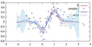
(a) Gaussian field regression $\hat{f}_{n}(\cdot)$ with range $\pm\sqrt{\hat{K}(\cdot)}$ given by (2.5)

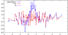
(b) The random weights $\lambda\,\hat{w}_{i}$ and the adapted noise $f_{i}-f_{\lambda}(X_{i})$ are almost comonotonic.

Figure 1: Approximation of functions for a sample of size $n=100$

Lemma 5.3.

The residuals are $\tilde{r}_{i}=\tilde{r}_{n}(X_{i})$.

Proof.

Indeed,

$$\tilde{r}_{i}=f_{i}-\lambda\,\frac{f_{i}-f_{\lambda}(X_{i})}{\lambda}-\frac{1}{n}\sum_{j=1}^{n}k(X_{i},X_{j})\,\tilde{w}_{j}=f_{\lambda}(X_{i})-\frac{1}{n}\sum_{j=1}^{n}k(X_{i},X_{j})\,\tilde{w}_{j}=\tilde{r}_{n}(X_{i}),$$

the assertion. ∎

We shall establish the relation between $\tilde{f}_{n}(\cdot)$ and $f_{\lambda}(\cdot)$ first. To this end recall that $\tilde{f}_{n}(\cdot)$ is random, while $f_{\lambda}(\cdot)$ is deterministic. The function $\tilde{f}_{n}(\cdot)$ recovers the function $f_{\lambda}(\cdot)$ on average and enjoys the following statistical properties.

Proposition 5.4 ($\tilde{f}_{n}$ is $f_{\lambda}$ on average).

It holds that

$$f_{\lambda}(x)=\operatorname{{\mathds{E}}}\tilde{f}_{n}(x),\qquad x\in\mathcal{X}.$$

Equivalently, the residual $\tilde{r}(\cdot)$ is locally unbiased, i.e.,

$$\operatorname{{\mathds{E}}}\tilde{r}_{n}(x)=0$$

for every $x\in\mathcal{X}$.

Proof.

Observe first with (3.2) and (3.9) that

$$\operatorname{{\mathds{E}}}\left(\left.\tilde{w}_{j}\right|X_{j}=x\right)=\operatorname{{\mathds{E}}}\left(\left.\frac{f_{j}-f_{\lambda}(X_{j})}{\lambda}\right|X_{j}=x\right)=\frac{f_{0}(x)-f_{\lambda}(x)}{\lambda}=w_{\lambda}(x)$$ (5.2)

as both, $f_{j}$ and $f_{\lambda}(X_{j})$ are in $L^{2}$. By the tower property of the expectation, by taking out what is known and (3.8),

$$\operatorname{{\mathds{E}}}k(x,X_{j})\,\tilde{w}_{j}=\operatorname{{\mathds{E}}}\left(k(x,X_{j})\operatorname{{\mathds{E}}}(\tilde{w}_{j}|\,X_{j})\right)=\operatorname{{\mathds{E}}}k(x,X_{j})\,w_{\lambda}(X_{j})=f_{\lambda}(x)$$ (5.3)

for every $j=1,\dots,n$. With this, the assertion is immediate and the expected value of the residual follows together with its definition in (5.1). ∎

The preceding relation reveals the expectation of $\tilde{f}_{n}$ locally. The next proposition demonstrates local convergence for increasing sample size $n$.

Proposition 5.5 (Local approximation quality).

For every $x\in\mathcal{X}$ there is a constant $C(x)>0$ so that

$$\operatorname{var}\tilde{f}_{n}(x)=\frac{C(x)}{n}.$$

Proof.

Employing Proposition 5.4 we have that

$$\operatorname{var}\tilde{f}_{n}(x) =\operatorname{{\mathds{E}}}\Big{(}f_{\lambda}(x)-\frac{1}{n}\sum_{j=1}^{n}\tilde{w_{j}}\,k(x,X_{j})\Big{)}^{2}$$

$$=f_{\lambda}(x)^{2}-2f_{\lambda}(x)^{2}+\frac{1}{n^{2}}\sum_{i,j=1}^{n}\operatorname{{\mathds{E}}}\tilde{w}_{i}\,\tilde{w}_{j}\,k(x,X_{i})\,k(x,X_{j})$$

$$=f_{\lambda}(x)^{2}-2f_{\lambda}(x)^{2}+\frac{n^{2}-n}{n^{2}}f_{\lambda}(x)^{2}+\frac{n}{n^{2}}\sum_{i=1}^{n}\operatorname{{\mathds{E}}}\Big{(}\frac{f_{i}-f_{\lambda}(X_{i})}{\lambda}\Big{)}^{2}k(x,X_{i})^{2}$$

as $X_{i}$ and $X_{j}$ are independent for $i\not=j$. It follows that $\operatorname{var}\tilde{f}_{n}(x)=-\frac{1}{n}f_{\lambda}(x)^{2}+\frac{1}{n\,\lambda^{2}}C^{\prime}(x)$, where $C^{\prime}(x)=\operatorname{{\mathds{E}}}\big{(}f-f_{\lambda}(X)\big{)}^{2}\,k(x,X)^{2}$ is finite. ∎

5.2 Uniform approximation properties of the auxiliary estimator $\tilde{f}_{n}$

The following theorem reveals the precise approximation quality of the estimator with weights $\tilde{w}$.

Theorem 5.6 (Approximation in norm).

It holds that

$$\operatorname{{\mathds{E}}}\|f_{\lambda}-\tilde{f}_{n}\|_{k}^{2}=\frac{C_{1}}{\lambda^{2}\,n},$$

where $C_{1}>0$ is a constant independent on $\lambda$ and $n$. More explicitly,

$$\operatorname{{\mathds{E}}}\left\|\tilde{r}_{n}\right\|_{k}^{2}=\frac{1}{\lambda^{2}\,n}\int_{\mathcal{X}}\Big{(}\operatorname{var}(f|\,x)+\big{(}f_{0}(x)-f_{\lambda}(x)\big{)}^{2}\Big{)}k(x,x)P(dx)-\frac{1}{n}\left\|f_{\lambda}\right\|_{k}^{2},$$

where $\operatorname{var}\big{(}f|\,x\big{)}=\operatorname{{\mathds{E}}}\Big{(}\big{(}f-f_{0}(X)\big{)}^{2}\big{|}\,X=x\Big{)}$ is the variance of the random data at $x$ (see (3.2)), the local irreducible error.

Remark 5.7.

The conditional variance term $\operatorname{var}(f|\,x)$ points to the fact that convergence actually differs for homoscedastic and heteroscedastic random observations $(X_{i},f_{i})$, $i=1,\dots,n$.

Proof.

With $f_{\lambda}=Kw_{\lambda}$ (cf. (3.8)) we have that

$$\operatorname{{\mathds{E}}}\biggl{\|}f_{\lambda}(\cdot)-\frac{1}{n}\sum_{j=1}^{n}k(\cdot,X_{j})\,\tilde{w}_{j}\biggr{\|}_{k}^{2}$$

$$=\operatorname{{\mathds{E}}}\left\|f_{\lambda}\right\|_{k}^{2}-2\biggl{\langle}f_{\lambda}\biggl{|}\,\frac{1}{n}\sum_{j=1}^{n}k(\cdot,X_{j})\,\tilde{w}_{j}\biggr{\rangle}_{k}+\biggl{\|}\frac{1}{n}\sum_{j=1}^{n}k(\cdot,X_{j})\,\tilde{w}_{j}\biggr{\|}_{k}^{2}$$

$$=\left\|f_{\lambda}\right\|_{k}^{2}$$

$$\qquad-2\operatorname{{\mathds{E}}}\frac{1}{n}\sum_{j=1}^{n}\int_{\mathcal{X}}w_{\lambda}(y)\,k(y,X_{j})\,\tilde{w}_{j}\,P(dy)$$ (5.4)

$$\qquad+\frac{1}{n^{2}}\sum_{i,j=1}^{n}\operatorname{{\mathds{E}}}\tilde{w}_{i}\,k(X_{i},X_{j})\,\tilde{w}_{j}.$$ (5.5)

With (5.3) and (2.9), the term (5.4) is

$$\operatorname{{\mathds{E}}}\frac{2}{n}\sum_{i=1}^{n}\int_{\mathcal{X}}w_{\lambda}(y)\,k(y,X_{j})\,\tilde{w}_{j}P(dy)=2\int_{\mathcal{X}}w_{\lambda}(y)\,f_{\lambda}(y)\,P(dy)=2\left\|f_{\lambda}\right\|_{k}^{2}.$$

For the remaining term (5.5) involving all combinations and by separating all combinations with $j=i$ from those with $j\not=i$ we find

$$\frac{1}{n^{2}}\sum_{i,j=1}^{n}\operatorname{{\mathds{E}}}\tilde{w}_{i}\,k(X_{i},X_{j})\,\tilde{w}_{j}=$$

$$=\frac{1}{n^{2}}\sum_{i=1}^{n}\operatorname{{\mathds{E}}}\operatorname{{\mathds{E}}}\Big{(}\Big{(}\frac{f_{i}-f_{\lambda}(X_{i})}{\lambda}\bigg{)}^{2}k(X_{i},X_{i})\biggr{|}X_{i}\bigg{)}+\frac{1}{n}\sum_{i=1}^{n}\frac{1}{n}\operatorname{{\mathds{E}}}\operatorname{{\mathds{E}}}\bigg{(}\tilde{w}_{i}\sum_{j\not=i}k(X_{i},X_{j})\,\tilde{w}_{j}\biggr{|}X_{i}\bigg{)}$$

$$=\frac{1}{n^{2}\lambda^{2}}\sum_{i=1}^{n}\operatorname{{\mathds{E}}}\operatorname{{\mathds{E}}}\Big{(}\big{(}f_{i}-f_{0}(X_{i})\big{)}^{2}+\big{(}f_{0}(X_{i})-f_{\lambda}(X_{i})\big{)}^{2}\biggr{|}X_{i}\bigg{)}\,k(X_{i},X_{i})$$

$$\qquad+\frac{1}{n}\sum_{i=1}^{n}\frac{1}{n}\operatorname{{\mathds{E}}}\operatorname{{\mathds{E}}}\bigg{(}\left(\frac{f_{i}-f_{0}(X_{i})}{\lambda}+\frac{f_{0}(X_{i})-f_{\lambda}(X_{i})}{\lambda}\right)\sum_{j\not=i}k(X_{i},X_{j})\,\tilde{w}_{j}\biggr{|}X_{i}\bigg{)},$$

as $2\operatorname{{\mathds{E}}}\Big{(}\big{(}f_{i}-f_{0}(X_{i})\big{)}\big{(}f_{0}(X_{i})-f_{\lambda}(X_{i})\big{)}\biggr{|}X_{i}\bigg{)}=0$ by the orthogonality relation (3.3).

With the kernel trick (see Mercer’s theorem in Remark 2.5), and independence of $(X_{i},f_{i})$ from $(X_{j},f_{j})$ for $j\not=i$ we have that

$$\operatorname{{\mathds{E}}}\operatorname{{\mathds{E}}}\bigg{(}\frac{f_{i}-f_{0}(X_{i})}{\lambda}k(X_{i},X_{j})\,\tilde{w}_{j}\biggr{|}X_{i}\bigg{)} =\sum_{\ell=1}^{\infty}\operatorname{{\mathds{E}}}\bigg{(}\frac{f_{i}-f_{0}(X_{i})}{\lambda}\sigma_{\ell}^{2}\phi_{\ell}(X_{i})\phi_{\ell}(X_{j})\,\tilde{w}_{j}\bigg{)}$$

$$=\sum_{\ell=1}^{\infty}\sigma_{\ell}^{2}\operatorname{{\mathds{E}}}\bigg{(}\frac{f_{i}-f_{0}(X_{i})}{\lambda}\phi_{\ell}(X_{i})\bigg{)}\operatorname{{\mathds{E}}}\bigg{(}\phi_{\ell}(X_{j})\,\tilde{w}_{j}\bigg{)}.$$

Again, by the orthogonality relation (2.5) we concluded that $\operatorname{{\mathds{E}}}\Big{(}\frac{f_{i}-f_{0}(X_{i})}{\lambda}\phi_{\ell}(X_{i})\Big{)}=0$. Summing up we have

$$\frac{1}{n^{2}}\sum_{i,j=1}^{n}\operatorname{{\mathds{E}}}\tilde{w}_{i}\,k(X_{i},X_{j})\,\tilde{w}_{j}=$$

$$=\frac{1}{n^{2}\lambda^{2}}\sum_{i=1}^{n}\operatorname{{\mathds{E}}}\operatorname{{\mathds{E}}}\Big{(}\big{(}f_{i}-f_{0}(X_{i})\big{)}^{2}+\big{(}f_{0}(X_{i})-f_{\lambda}(X_{i})\big{)}^{2}\biggr{|}X_{i}\bigg{)}\,k(X_{i},X_{i})$$

$$\qquad+\frac{1}{n}\sum_{i=1}^{n}\frac{1}{n}\operatorname{{\mathds{E}}}\frac{f_{0}(X_{i})-f_{\lambda}(X_{i})}{\lambda}\sum_{j\not=i}\operatorname{{\mathds{E}}}\bigg{(}k(X_{i},X_{j})\,\tilde{w}_{j}\biggr{|}X_{i}\bigg{)}$$

$$=\frac{1}{n^{2}\lambda^{2}}\sum_{i=1}^{n}\operatorname{{\mathds{E}}}\Big{(}\operatorname{var}(f\mid X_{i})+\big{(}f_{0}(X_{i})-f_{\lambda}(X_{i})\big{)}^{2}\bigg{)}k(X_{i},X_{i})$$

$$\qquad+\frac{1}{n}\sum_{i=1}^{n}\frac{1}{n}\sum_{j\not=i}\operatorname{{\mathds{E}}}w_{\lambda}(X_{i})\,f_{\lambda}(X_{i}),$$

where we have employed (5.3) again. As above, we have again that

$$\operatorname{{\mathds{E}}}w_{\lambda}(X_{i})f_{\lambda}(X_{i})=\left\|f_{\lambda}\right\|_{k}^{2}.$$

Collecting terms we find that

$$\operatorname{{\mathds{E}}}\biggl{\|}f_{\lambda}(\cdot)-\frac{1}{n}\sum_{j=1}^{n}k(\cdot,X_{j})\,\tilde{w}_{j}\biggr{\|}_{k}^{2}=\left\|f_{\lambda}\right\|_{k}^{2}-2\left\|f_{\lambda}\right\|_{k}^{2}$$

$$+\frac{n-1}{n}\left\|f_{\lambda}\right\|_{k}^{2}+\frac{1}{\lambda^{2}n}\int_{\mathcal{X}}\Big{(}\operatorname{var}(f|\,x)+\big{(}f_{0}(x)-f_{\lambda}(x)\big{)}^{2}\Big{)}k(x,x)P(dx)$$

and thus the assertion. ∎

Remark 5.8 (Local correlation).

The coefficients $\tilde{w}_{i}$ depend explicitly on $f_{i}$. This explicit relation will actually allow us to dampen, even to remove the noise from the estimators. Indeed, the noise $f_{i}$ and the coefficients $\tilde{w}_{i}$ are utmost correlated, it holds that

$$\operatorname{corr}(f_{i},\tilde{w}_{i}\mid X_{i}=x)=1.$$ (5.6)

To accept this strong correlation property recall the relation $\tilde{w}_{i}=\frac{1}{\lambda}f_{i}+\frac{1}{\lambda}f_{\lambda}(X_{i})$, which exhibits—provided that $X_{i}=x$ is kept fixed—an affine relation between $\tilde{w}_{i}$ and $f_{i}$ and thus (5.6).

5.3 The relation of the SAA estimator $\hat{f}_{n}$ and $\tilde{f}_{n}$

The unbiased estimator $\tilde{f}_{n}$ and the estimator of interest $\hat{f}_{n}$ are connected explicitly in the following way.

Lemma 5.9.

It holds that

$$\hat{f}_{n}(\cdot)-\tilde{f}_{n}(\cdot)=\frac{1}{n}\sum_{j=1}^{n}\tilde{r}_{n}^{\top}\Big{(}\lambda+\frac{1}{n}K\Big{)}_{j}^{-1}\,k(\cdot,X_{j})$$

and

$$\|\hat{f}_{n}-\tilde{f}_{n}\|_{k}^{2}=\frac{1}{n}\tilde{r}^{\top}\Big{(}\lambda+\frac{1}{n}K\Big{)}^{-1}\,\frac{1}{n}K\,\Big{(}\lambda+\frac{1}{n}K\Big{)}^{-1}\tilde{r};$$ (5.7)

here, $K$ is the random Gramian matrix with entries $K_{ij}=k(X_{i},X_{j})$.

Proof.

By the definition of $\tilde{r}_{i}$ and (4.3),

$$\tilde{r}_{i} =f_{i}-\lambda\,\tilde{w}_{i}-\frac{1}{n}\sum_{j=1}^{n}k(X_{i},X_{j})\,\tilde{w}_{j}$$

$$=\lambda\,\hat{w}_{i}+\frac{1}{n}\sum_{j=1}^{n}k(X_{i},X_{j})\hat{w}_{j}-\lambda\,\tilde{w}_{i}-\frac{1}{n}\sum_{j=1}^{n}k(X_{i},X_{j})\,\tilde{w}_{j}$$

$$=\Big{(}\lambda+\frac{1}{n}K\Big{)}_{i}(\hat{w}-\tilde{w})$$

and thus

$$\hat{w}-\tilde{w}=\Big{(}\lambda+\frac{1}{n}K\Big{)}^{-1}\tilde{r}.$$

Now recall that $\hat{f}_{n}(\cdot)-\tilde{f}_{n}(\cdot)=\frac{1}{n}\sum_{j=1}^{n}(\hat{w}_{j}-\tilde{w}_{j})\,k(\cdot,X_{j})$ and the definition of the inner product $\left\langle\cdot\mid\cdot\right\rangle_{k}$ to accept the remaining assertion. ∎

In what follows we provide the relation between the estimator of interest $\hat{f}$ and the auxiliary estimator $\tilde{f}$. The following Lemma is essential, it allows to get rid of the random matrix $K$ and its inverse in (5.7).

Lemma 5.10.

For any nonnegative definite matrix $K$ (i.e., $K\geq 0$) it holds that

$$\big{(}\lambda+K\big{)}^{-1}K\big{(}\lambda+K\big{)}^{-1}\leq\frac{1}{4\lambda}$$ (5.8)

in Loewner order.

Proof.

It holds that $0\leq(\lambda-K)^{2}=\lambda^{2}-2\lambda K+K^{2}$ and thus $4\lambda K\leq\lambda^{2}+2\lambda K+K^{2}=(\lambda+K)^{2}$. The assertion follows after multiplying with the corresponding inverse from left and right. ∎

Proposition 5.11.

It holds that

$$\operatorname{{\mathds{E}}}\|\hat{f}_{n}-\tilde{f}_{n}\|_{k}^{2}\leq\frac{C_{2}}{4\lambda^{3}n}$$ (5.9)

for a constant $C_{2}>0$ independent of $\lambda$ and $n$.

Proof.

From (5.7) and Lemma 5.10, applied to the matrix $\frac{1}{n}K$, we conclude that

$$\|\hat{f}_{n}-\tilde{f}_{n}\|_{k}^{2}=\frac{1}{n}\tilde{r}^{\top}\Big{(}\lambda+\frac{1}{n}K\Big{)}^{-1}\frac{1}{n}K\Big{(}\lambda+\frac{1}{n}K\Big{)}^{-1}\tilde{r}\leq\frac{1}{4\lambda}\cdot\frac{1}{n}\tilde{r}^{\top}\tilde{r}.$$ (5.10)

With Lemma 5.3 it follows that

$$\operatorname{{\mathds{E}}}\|\hat{f}_{n}-\tilde{f}_{n}\|_{k}^{2}\leq\frac{1}{4\lambda}\cdot\frac{1}{n}\sum_{i=1}^{n}\operatorname{{\mathds{E}}}\tilde{r}_{n}(X_{i})^{2}=\frac{1}{4\lambda}\cdot\operatorname{{\mathds{E}}}\tilde{r}_{n}(X_{i})^{2}$$

for any $i=1,\dots,n$. Employing the definition of $\tilde{r}_{n}(\cdot)$ (cf. (5.1)) the right hand side expression expands as

$$\operatorname{{\mathds{E}}}\tilde{r}_{n}(X_{i})^{2} =\operatorname{{\mathds{E}}}\left(f_{\lambda}(X_{i})-\frac{1}{n}\sum_{j=1}^{n}k(X_{i},X_{j})\frac{f_{j}-f_{\lambda}(X_{j})}{\lambda}\right)^{2}$$

$$=\operatorname{{\mathds{E}}}f_{\lambda}(X_{i})^{2}$$

$$\qquad-\frac{2}{n}\sum_{j=1}^{n}\operatorname{{\mathds{E}}}f_{\lambda}(X_{i})\cdot k(X_{i},X_{j})\frac{f_{j}-f_{\lambda}(X_{j})}{\lambda}$$ (5.11)

$$\qquad+\frac{1}{n^{2}}\sum_{j,\ell=1}^{n}\operatorname{{\mathds{E}}}k(X_{i},X_{j})\frac{f_{j}-f_{\lambda}(X_{j})}{\lambda}k(X_{i},X_{\ell})\frac{f_{\ell}-f_{\lambda}(X_{\ell})}{\lambda}.$$ (5.12)

We now treat (5.11) and (5.12) separately. As for the first term we have for $j\not=i$ that

$$\operatorname{{\mathds{E}}}f_{\lambda}(X_{i})\cdot k(X_{i},X_{j})\frac{f_{j}-f_{\lambda}(X_{j})}{\lambda}$$

$$=\operatorname{{\mathds{E}}}f_{\lambda}(X_{i})\operatorname{{\mathds{E}}}\bigg{(}\left.k(X_{i},X_{j})\frac{f_{j}-f_{\lambda}(X_{j})}{\lambda}\right|X_{i},X_{j}\bigg{)}$$

$$=\operatorname{{\mathds{E}}}f_{\lambda}(X_{i})\operatorname{{\mathds{E}}}\bigg{(}\left.k(X_{i},X_{j})\frac{f_{0}(X_{j})-f_{\lambda}(X_{j})}{\lambda}\right|X_{i}\bigg{)}$$

$$=\operatorname{{\mathds{E}}}f_{\lambda}(X_{i})\cdot\operatorname{{\mathds{E}}}\bigg{(}\left.k(X_{i},X_{j})\,w_{\lambda}(X_{j})\right|X_{i}\bigg{)}$$

$$=\operatorname{{\mathds{E}}}f_{\lambda}(X_{i})\cdot f_{\lambda}(X_{i})$$

$$=\operatorname{{\mathds{E}}}f_{\lambda}(X_{i})^{2},$$

where we have used (3.9). For $j=i$, the term (5.11) is

$$\operatorname{{\mathds{E}}}f_{\lambda}(X_{i})k(X_{i},X_{i})\frac{f_{0}(X_{i})-f_{\lambda}(X_{i})}{\lambda}=\operatorname{{\mathds{E}}}f_{\lambda}(X_{i})k(X_{i},X_{i})w_{\lambda}(X_{i}).$$

For the remaining term (5.12) and $i$, $j$ and $\ell$ all distinct we find that

$$\operatorname{{\mathds{E}}}\operatorname{{\mathds{E}}}\bigg{(}\left.k(X_{i},X_{j})\frac{f_{j}-f_{\lambda}(X_{j})}{\lambda}k(X_{i},X_{\ell})\frac{f_{\ell}-f_{\lambda}(X_{\ell})}{\lambda}\right|X_{i}\bigg{)}$$

$$=\operatorname{{\mathds{E}}}\operatorname{{\mathds{E}}}\bigg{(}\left.k(X_{i},X_{j})\frac{f_{0}(X_{j})-f_{\lambda}(X_{j})}{\lambda}\right|X_{i}\bigg{)}\operatorname{{\mathds{E}}}\bigg{(}\left.k(X_{i},X_{\ell})\frac{f_{0}(X_{\ell})-f_{\lambda}(X_{\ell})}{\lambda}\right|X_{i}\bigg{)}$$

$$=\operatorname{{\mathds{E}}}\operatorname{{\mathds{E}}}\bigg{(}\left.k(X_{i},X_{j})w_{\lambda}(X_{j})\right|X_{i}\bigg{)}\operatorname{{\mathds{E}}}\bigg{(}\left.k(X_{i},X_{\ell})w_{\lambda}(X_{\ell})\right|X_{i}\bigg{)}$$

$$=\operatorname{{\mathds{E}}}f_{\lambda}(X_{i})^{2},$$

as $X_{j}$ and $X_{\ell}$ are independent.

There are $2n-1$ out of $n^{2}$ combinations when not all $i$, $j$ and $\ell$ are distinct, in which case the expression (5.12) is finite with factor $\frac{1}{\lambda^{2}}$ only if $j=\ell$. Collecting now all terms and connecting with (5.10) reveals the assertion (5.9) of the theorem. ∎

The elementary relation in Lemma 5.10 is of crucial importance in the preceding proof, as it allows to get rid of the random matrices $\lambda+\frac{1}{n}K$ and, even more importantly, its inverse. We discuss some situations, where the bound can be improved.

Remark 5.12.

Suppose the kernel function is uniformly bounded from below,

$$k(\cdot,:)\geq k_{\mathit{min}}>0$$ (5.13)

$P^{2}$-almost everywhere on $\mathcal{X}\times\mathcal{X}$. Then the assertion of Proposition 5.11 is

$$\operatorname{{\mathds{E}}}\|\hat{f}_{n}-\tilde{f}_{0}\|_{k}\leq\frac{C_{2}}{k_{\mathit{min}}\,\lambda^{2}\,n}.$$

Indeed, observe first that $k_{\mathit{min}}\,K\leq K^{2}\leq(\lambda+K)(\lambda+K)$ so that

$$\big{(}\lambda+K\big{)}^{-1}K\big{(}\lambda+K\big{)}^{-1}\leq\frac{1}{k_{\mathit{min}}}.$$ (5.14)

The same proof as Proposition 5.11 applies (with (5.8) replaced by (5.14)) and we conclude with

$$\operatorname{{\mathds{E}}}\|\hat{f}_{n}-\tilde{f}_{n}\|_{k}^{2}\leq\frac{1}{k_{\mathit{min}}\,\lambda^{2}n}.$$ (5.15)

Note that the assumption particularly implies that the support $\operatorname{supp}P$ is compact in $\mathcal{X}$ (see Footnote 3 on page 3). But kernel functions $k$, which are not compactly supported, enjoy the property (5.13) on compact subsets of $\mathcal{X}$ so that this assumption is not unusual in applications.

Remark 5.13.

The inequality (5.8) is crucial in the analysis above as it allows to get rid of the inverse of a matrix with random coefficients. We assume that a better estimate at this point will likely improve the quality of the approximation as in (5.15); perhaps the estimates on eigenvalues presented by Shawe-Taylor et al. [18] can be of help to improve the inequality.

6 Convergence in norm and consistency

We can now connect the auxiliary and partial results of the preceding sections to present our main results. They identify the limit in the initial problem (2.3) and describe convergence of the estimator $\hat{f}_{n}$ towards $f_{\lambda}$ and towards $f_{0}$, as well as consistency of the estimators.

6.1 Convergence in norm

The estimator $\hat{f}_{n}$ converges to $f_{\lambda}$ in expected norm, as the sample size increases.

Theorem 6.1.

For the estimator $\hat{f}_{n}(\cdot)$ it holds that $\operatorname{{\mathds{E}}}\|\hat{f}_{n}-f_{\lambda}\|_{k}^{2}\leq\frac{2C_{1}}{\lambda^{2}\,n}+\frac{C_{2}}{\lambda^{3}\,n}$, where $C_{1}$ and $C_{2}>0$ are constants independent of $\lambda$ and $n$.

Proof.

By the triangle inequality, Theorem 5.6 and Proposition 5.11 we find that

$$\operatorname{{\mathds{E}}}\|\hat{f}_{n}-f_{\lambda}\|_{k}^{2} \leq\operatorname{{\mathds{E}}}\big{(}\|f_{\lambda}-\tilde{f}_{n}\|_{k}+\|\tilde{f}_{n}-\hat{f}_{n}\|_{k}\big{)}^{2}$$

$$\leq 2\operatorname{{\mathds{E}}}\|f_{\lambda}-\tilde{f}_{n}\|_{k}^{2}+2\operatorname{{\mathds{E}}}\|\tilde{f}_{n}-\hat{f}_{n}\|_{k}^{2}$$

$$\leq\frac{2C_{1}}{\lambda^{2}\,n}+\frac{C_{2}}{2\lambda^{3}\,n},$$

the assertion. ∎

Corollary 6.2 (Convergence in $L^{2}$).

It holds that $\operatorname{{\mathds{E}}}\|\hat{f}_{n}-f_{\lambda}\|_{2}^{2}\leq\frac{2C_{1}}{\lambda^{2}\,n}+\frac{C_{2}}{\lambda^{3}\,n}$, where $C_{1}$ and $C_{2}>0$ are constants independent of $\lambda$ and $n$.

Proof.

The assertion is immediate with Proposition 2.6. ∎

Theorem 6.3.

Suppose that $f_{0}=Kw_{0}$ with $w_{0}\in\mathcal{H}_{k}$ so that $f_{0}$ is in the Hilbert space $\mathcal{H}_{k}$ as well. Then there are constants $C_{0}$, $C_{1}$ and $C_{2}$, all independent of $n$ and $\lambda$, so that

$$\operatorname{{\mathds{E}}}\|f_{0}-\hat{f}_{n}\|_{k}^{2}\leq 2C_{0}\lambda^{2}+\frac{4C_{1}}{\lambda^{2}\,n}+\frac{C_{2}}{\lambda^{3}\,n}.$$ (6.1)

Proof.

By involving Proposition 3.5 in combination with Theorem 6.1 we have that

$$\operatorname{{\mathds{E}}}\|f_{0}-\hat{f}_{n}\|_{k}^{2} \leq\operatorname{{\mathds{E}}}\big{(}\|f_{0}-f_{\lambda}\|_{k}+\|\hat{f}_{n}-f_{\lambda}\|_{k}\big{)}^{2}$$

$$\leq 2\|f_{0}-f_{\lambda}\|_{k}^{2}+2\operatorname{{\mathds{E}}}\|\hat{f}_{n}-f_{\lambda}\|_{k}^{2}$$

$$\leq 2\lambda^{2}\|w_{0}\|_{k}^{2}+\frac{4C_{1}}{\lambda^{2}\,n}+\frac{C_{2}}{\lambda^{3}\,n}$$

and hence the assertion with $C_{0}\coloneqq\|w_{0}\|_{k}^{2}$. ∎

As above, we have the following corollary.

Corollary 6.4 (Convergence in $L^{2}$).

For $f_{0}=Kw_{0}\in\mathcal{H}_{k}$ there are constants $C_{0}$, $C_{1}$ and $C_{2}$, all independent of $n$ and $\lambda$, so that that

$$\operatorname{{\mathds{E}}}\|f_{0}-\hat{f}_{n}\|_{2}^{2}\leq C_{0}\,\lambda^{2}+\frac{4C_{1}}{\lambda^{2}\,n}+\frac{C_{2}}{\lambda^{3}\,n}.$$

Proof.

Just recall that the norm in $L^{2}$ is $\|f\|_{2}^{2}=\operatorname{{\mathds{E}}}|f|^{2}$. ∎

6.2 Asymptotically optimal convergence rates and uniform approximation

The results in the preceding section exhibit the typical bias variance problem: the parameter $\lambda$ in (6.1), for example, should be small to increase the approximation quality of $f_{\lambda}$ for $f_{0}$; on the other side, $\lambda$ should be large to improve the approximation of $f_{\lambda}$ and the estimator $\hat{f}_{n}$. The following statements reveal the best approximation rates asymptotically.

Theorem 6.5.

For $f_{0}$ in the range of $K$ and $\lambda_{n}=C\cdot n^{-\nicefrac{{1}}{{5}}}$ it holds that

$$\operatorname{{\mathds{E}}}\|f_{0}-\hat{f}_{n}\|_{k}^{2}\leq\frac{C}{n^{\nicefrac{{2}}{{5}}}}.$$

Proof.

The assertion derives from (6.1). ∎

The following corollary is again immediate with Proposition 2.6.

Corollary 6.6 (Convergence in $L^{2}$).

For $f_{0}=Kw_{0}$ it holds that

$$\operatorname{{\mathds{E}}}\|f_{0}-\hat{f}_{n}\|_{2}^{2}\leq\mathcal{O}\big{(}n^{-\nicefrac{{2}}{{5}}}\big{)},$$

provided that $\lambda_{n}=\mathcal{O}\big{(}n^{-\nicefrac{{1}}{{5}}}\big{)}$.

Remark 6.7.

Assuming (5.13) we found the slower rate (5.15). With that, the leading term is $\frac{C}{\lambda^{2}n}$ instead of $\frac{C}{\lambda^{2}n}$ in (6.1) and the optimal rate is

$$\operatorname{{\mathds{E}}}\|f_{0}-\hat{f}_{n}\|_{k}^{2}\leq\frac{C}{n^{\nicefrac{{1}}{{2}}}}$$

and by Jensen’s inequality and (2.10) thus

$$C_{k}^{-1}\|f_{0}-\hat{f}_{n}\|_{\infty}\leq\operatorname{{\mathds{E}}}\|f_{0}-\hat{f}_{n}\|_{k}\leq\frac{C}{n^{\nicefrac{{1}}{{4}}}}$$

for $\lambda=\mathcal{O}\big{(}n^{-\nicefrac{{1}}{{2}}}\big{)}$, where $C_{k}\coloneqq\sup_{x\in\operatorname{supp}P}\sqrt{k(x,x)}$.

6.3 Weak consistency

We have seen in Theorem 4.4 that the estimator $\hat{\vartheta}_{n}$ of the objective is downwards biased. However, weak consistency of the estimator $\hat{\vartheta}_{n}$ is immediate as the optimizers converge.

Theorem 6.8.

Given the conditions of Theorem 6.3 it holds that $\hat{f}_{n}$ converges to $f_{0}$ in probability. Further, for every $x\in\mathcal{X}$, $\hat{f}_{n}(x)\to f_{0}(x)$, as $n\to\infty$, in probability.

Proof.

Indeed, by Markov’s inequality,

$$P\big{(}\|f_{0}-\hat{f}_{n}\|_{k}\geq\varepsilon\big{)}\leq\frac{1}{\varepsilon^{2}}\operatorname{{\mathds{E}}}\|f_{0}-\hat{f}_{n}\|_{k}^{2}\to 0,$$

as $n\to\infty$ and thus the assertion is immediate. ∎

Theorem 6.9.

The estimators $\hat{\vartheta}_{n}$ are $L^{2}$-consistent.

Proof.

The assertion is immediate by Theorem 2.6 and the fact that $\hat{f}_{n}$ is optimal for $\hat{\vartheta}_{n}$ in (4.1). ∎

7 Discussion and summary

This paper addresses the regression problem to learn or reconstruct a function, the conditional expectation function, from data observed with noise. The method investigates an unbiased functional estimator, which reconstructs the desired function under general preconditions. This estimator is closely related to a popular estimator employed in machine learning, for which we develop a tight relation. We provide results for convergence in the norm of the genuine space, the norm associated with the reproducing kernel Hilbert space.

The norm of the reproducing kernel Hilbert space is stronger than uniform convergence. For this reason, the results allow to estimate functions and establish their uniform convergence. With that, the results are just appropriate for applications in stochastic optimization, a subject with many intersections with neural networks and deep learning.

The convergence rates presented here are in line with other results in nonparametric statistics. However, we believe to have evidence from numerical computations that convergence rates can be improved and this is subject to forthcoming research. A further topic, which this paper does not touch, is the selection of the bandwidth. As well it would be interesting to find and characterize the limiting distribution.

Some of the results can be compared with the Nadaraya–Watson estimator (see Tsybakov [21] on kernel density estimation), which builds on kernels as well to estimator the conditional expectation. This method from nonparametric statistics has similar convergence properties and requires an oracle on the density function to find optimal convergence rates.

Finally we want to mention that we have an implementation available at github,

https://github.com/aloispichler/reproducing-kernel-Hilbert-space,

which allows assessing the theoretical results of the paper numerically.

8 Acknowledgment

We wish to thank Prof. Alexander Shapiro, Georgia Tech, and Prof. Tino Ullrich, TU Chemnitz, for discussion on a draft version of the manuscript.

References

- Ambrosio et al. [2005] L. Ambrosio, N. Gigli, and G. Savaré. Gradient Flows in Metric Spaces and in the Space of Probability Measures. Birkhäuser Verlag, Basel, Switzerland, 2 edition, 2005. doi:10.1007/978-3-7643-8722-8.
- Bach [2013] F. Bach. Sharp analysis of low-rank kernel matrix approximations. In S. Shalev-Shwartz and I. Steinwart, editors, Proceedings of the 26th Annual Conference on Learning Theory, volume 30 of Proceedings of Machine Learning Research, pages 185–209, Princeton, NJ, USA, 2013. PMLR. URL http://proceedings.mlr.press/v30/Bach13.html.
- Bishop [2006] C. M. Bishop. Pattern Recognition and Machine Learning. Springer-Verlag New York Inc., 2006. ISBN 0387310738. URL https://www.springer.com/de/book/9780387310732.
- Caponnetto and De Vito [2006] A. Caponnetto and E. De Vito. Optimal rates for the regularized least-squares algorithm. Foundations of Computational Mathematics, 7(3):331–368, 2006. doi:10.1007/s10208-006-0196-8.
- Cucker and Zhou [2015] F. Cucker and D.-X. Zhou. Learning Theory: An Approximation Theory Viewpoint. Cambridge University Press, 2015. ISBN 0511274076. doi:10.1017/CBO9780511618796.
- Dellacherie and Meyer [1988] C. Dellacherie and P.-A. Meyer. Probabilities and Potential. North-Holland Publishing Co., Amsterdam, The Netherlands., 1988. URL https://projecteuclid.org/euclid.bams/1183546371.
- Györfi et al. [2002] L. Györfi, M. Kohler, A. Krzyżak, and H. Walk. A Distribution-Free Theory of Nonparametric Regression. Springer New York, 2002. doi:10.1007/b97848.
- Hein and Bousquet [2004] M. Hein and O. Bousquet. Kernels, associated structures and generalizations. Technical Report 127, Max Planck Institute for Biological Cybernetics, Tübingen, Germany, 2004. URL http://is.tuebingen.mpg.de/fileadmin/user_upload/files/publications/pdf2816.pdf.
- Kallenberg [2002] O. Kallenberg. Foundations of Modern Probability. Springer, New York, 2002. doi:10.1007/b98838.
- König [1986] H. König. Eigenvalue Distribution of Compact Operators. Birkhäuser Basel, 1986. doi:10.1007/978-3-0348-6278-3.
- Mandrekar and Gawarecki [2015] V. S. Mandrekar and L. Gawarecki. Stochastic Analysis for Gaussian Random Processes and Fields. CRC Press, 2015. ISBN 9781498707817. doi:10.1201/b18622.
- Norkin et al. [1998] V. I. Norkin, G. Ch. Pflug, and A. Ruszczyński. A branch and bound method for stochastic global optimization. Mathematical Programming, 83(1-3):425–450, 1998. doi:10.1007/BF02680569.
- Reed and Simon [1980] M. Reed and B. Simon. Methods of modern mathematical physics. Academic Press, 1980. ISBN 0125850506.
- Rüschendorf [2014] L. Rüschendorf. Mathematische Statistik. Springer Berlin Heidelberg, 2014. doi:10.1007/978-3-642-41997-3.
- Schmidt [1907] E. Schmidt. Zur Theorie der linearen und nichtlinearen Integralgleichungen. 63:433–476, 1907. doi:10.1007/BF01449770.
- Schölkopf et al. [2001] B. Schölkopf, R. Herbrich, and A. J. Smola. A generalized representer theorem. In Lecture Notes in Computer Science, pages 416–426. Springer Berlin Heidelberg, 2001. doi:10.1007/3-540-44581-1_27.
- Shapiro et al. [2014] A. Shapiro, D. Dentcheva, and A. Ruszczyński. Lectures on Stochastic Programming. MOS-SIAM Series on Optimization. SIAM, second edition, 2014. doi:10.1137/1.9780898718751.
- Shawe-Taylor et al. [2005] J. Shawe-Taylor, C. K. I. Williams, N. Cristianini, and J. Kandola. On the eigenspectrum of the gram matrix and the generalization error of kernel-PCA. 51(7):2510–2522, 2005. doi:10.1109/tit.2005.850052.
- Shiryaev [1996] A. N. Shiryaev. Probability. Springer, New York, 1996. doi:10.1007/978-1-4757-2539-1.
- Steinwart and Christmann [2008] I. Steinwart and A. Christmann. Support Vector Machines. Springer New York, 2008. doi:10.1007/978-0-387-77242-4.
- Tsybakov [2008] A. B. Tsybakov. Introduction to Nonparametric Estimation. Springer, New York, 2008. doi:10.1007/b13794.
- Wendland [2004] H. Wendland. Scattered Data Approximation. Cambridge University Press, 2004. doi:10.1017/cbo9780511617539.
- Zhang et al. [2013] Y. Zhang, J. Duchi, and M. Wainwright. Divide and conquer kernel ridge regression. In S. Shalev-Shwartz and I. Steinwart, editors, Proceedings of the 26th Annual Conference on Learning Theory, volume 30 of Proceedings of Machine Learning Research, pages 592–617, Princeton, NJ, USA, 2013. PMLR. URL http://proceedings.mlr.press/v30/Zhang13.html.