Flexible Principal Component Analysis for Exponential Family Distributions

Abstract

Traditional principal component analysis (PCA) is well known in high-dimensional data analysis, but it requires to express data by a matrix with observations to be continuous. To overcome the limitations, a new method called flexible PCA (FPCA) for exponential family distributions is proposed. The goal is to ensure that it can be implemented to arbitrary shaped region for either count or continuous observations. The methodology of FPCA is developed under the framework of generalized linear models. It provides statistical models for FPCA not limited to matrix expressions of the data. A maximum likelihood approach is proposed to derive the decomposition when the number of principal components (PCs) is known. This naturally induces a penalized likelihood approach to determine the number of PCs when it is unknown. By modifying it for missing data problems, the proposed method is compared with previous PCA methods for missing data. The simulation study shows that the performance of FPCA is always better than its competitors. The application uses the proposed method to reduce the dimensionality of arbitrary shaped sub-regions of images and the global spread patterns of COVID-19 under normal and Poisson distributions, respectively.

AMS 2000 Subject Classification: 62H25; 62H35, 62J05

Key Words: COVID-19; Dimension Reduction; Exponential Family Distributions; Image Analysis; Maximum Likelihood; Flexible Principal Component Analysis.

1 Introduction

Principal component analysis (PCA) is a well known dimension reduction technique in high-dimensional data analysis if continuous observations can be expressed by a data matrix. Previous PCA methods rely on a matrix technique called singular value decomposition (SVD). SVD decomposes the data matrix into the product of a left matrix for the left singular vectors, a diagonal matrix for singular values, and a right matrix for the right singular vectors. By removing small singular values with corresponding singular vectors from the output, a low-rank approximation of the input matrix, called traditional PCA, is derived. We have identified at least two limitations in this method. The first is that traditional PCA cannot be used if observations cannot be expressed by a data matrix. The second is that traditional PCA cannot be used even if observations can expressed by a data matrix but all of the observations are count. The goal of the research is to develop a new method, called flexible PCA (FPCA), to overcome the two limitations.

We emphasize the contribution of our method by Figure 1. If an image data has been loaded by a computer and the observations have been expressed by a matrix (Figure 1(a)), then traditional PCA can be implemented to the data. This is a widely used approach in image analysis because any black-and-white image can be treated as a matrix and any color image can be treated as a combination of three matrices for RGB channels, respectively. However, if the interest is not the entire image but only a specific region contained by the image, then it is inappropriate to use traditional PCA because irrelevant information contained by pixels outside the region is involved. To overcome the difficulty, dimension reduction for arbitrary shaped regions is needed (Figure 1(b)). In addition, if all of the entries of the matrix are count, then it is inappropriate to use traditional PCA in the case displayed by Figure 1(a) either. Therefore, we need to address two challenges. The first is to ensure that FPCA can be implemented to arbitrary shaped regions. The second is to ensure that it can be implemented to count data.

Figure 1: Shapes of regions can only be considered by traditional PCA for matrices (the left), but our proposed FPCA can consider arbitrary shaped regions (the right).

We avoid SVD in our method. Instead, we use the maximum likelihood approach, where we need a statistical model. The model is obtained by extensions of previous PCA models for matrices. Three PCA models have been proposed in the literature. The first is the low-rank mean model [1, P. 146]. The second is the latent factor model [28, 36]. The third is the spiked covariance model [23]. We devise our model by an extension of the low-rank mean model because the latent factor and the spiked covariance models contain matrix transformations, not easy to interpret for arbitrary shaped regions. In addition, the low-rank mean model has been extended to count matrices by the generalized linear models (GLMs) [7], leading to a method called generalized PCA [27]. Based on the maximum likelihood approach in the low-rank mean model for arbitrary shaped regions, we are able to address the two challenges that we have mentioned in the previous paragraph.

Our method is fundamentally different from previous PCA methods for missing values [13, 24], including generalized PCA [27]. We purposely discard observations outside of the region of interest even though they are available. Therefore, it is not a missing data problem. The previous methods assume that data are given by matrix forms. Missing values appear if some entries of the matrix are not available. Imputations for missing values are needed because they use SVD for the completed data to derive the decomposition. This often involves the mechanisms for generating missing data in the evaluation of their theoretical properties. However, missing data mechanism is not an issue and SVD is purposely avoided in our method.

In the literature, PCA [22] is a widely used dimension reduction technique for matrices data. Besides PCA, another often used technique is sufficient dimension reduction [9, 29]. The difference is that PCA does not need a response variable, but this is required in sufficient dimension reduction. Thus, PCA is an unsupervised learning method, but sufficient dimension reduction is not. Based on SVD for an input matrix, PCA can reduce the dimensionality of high-dimensional vector-valued variables of interest and simultaneously preserves their relationship [8, 30]. In the past a few decades, statistical approaches to dimension reduction have gained considerable attention due to rapid increases of data volume and dimension [10, 29, 38]. The implementation of dimension reduction techniques, including PCA, becomes popular in high-dimensional data analysis. Examples include dimension reduction in linear models [34], generalized linear models (GLMs) [32], discriminant analysis [6, 44], cluster analysis [18], image analysis [4, 21, 39], and big data [40, 41]. All of these methods assume that observations can be expressed by a matrix. PCA is an approximate method. It provides the best approximation based on the measure given by the Frobenius norm loss between the input matrix and the decomposition. This property naturally provides a regression model to interpret PCA. In FPCA, we use the maximum likelihood approach, including the least squares for the regression model, in the derivation. Therefore, our method is more flexible than previous PCA methods based on SVD.

Our method also includes the penalized likelihood approach for the determination of numbers of principal components (PCs). It recommends using the maximum likelihood approach to estimate the decomposition if the number of PCs is known. If the number of PCs is unknown, then we use the penalized likelihood approach. The development of the penalized likelihood approach is straightforward because the likelihood function is provided in each candidate models. In the literature, the determination of the number of PCs is considered as one of the most important problems in traditional PCA for matrices. This problem can be assessed by the penalized likelihood approach. By studying a few well known options of the tuning parameter in the penalized likelihood approach for variable selection, we conclude that the number of PCs can be determined by BIC but not AIC. This is consistent with a previous finding for the same problem when data can be expressed by a matrix [2]. Our research indicates that BIC can also be used to determine the number of PCs even if data cannot be expressed by a matrix.

The article is organized as follows. In Section 2, we introduce our method. In Section 3, by treating FPCA as a method for missing data, we compare our method with our competitors by simulations. The simulation results show that the performance of our method is always better than our competitors. In Section 4, we implement our method to three real world examples. Two are image analysis problems. One is an infectious disease problem. It is dimension reduction for the outbreak of COVID-19 in the world. In Section 5, we provide a discussion.

2 Method

We propose statistical models for FPCA in Section 2.1. We propose maximum likelihood estimation to derive the FPCA decomposition based on a selected number of PCs in Section 2.2. Because the determination of the number of PCs is important in PCA even for matrices, we propose a penalized likelihood approach to estimate the number of PCs in Section 2.3. Although our method is not proposed for missing data problem, it can be modified for such a problem. This is introduced in Section 2.4.

2.1 Statistical Model for FPCA

We propose our statistical model for FPCA by modifications of previous models for matrices. In the literature, three PCA models have been proposed for matrices. All of them assume that the number of PCs, denoted by $k$, is known. The first is the low-rank mean model [1]. It assumes that the data matrix is equal to the sum of the low-rank matrix and a white noise error matrix. The second is the latent factor model [28, 36]. It assumes that the data matrix is derived by a common transformation on a number of iid multivariate normal latent random factors. The third is the spiked covariance model [23]. It assumes that singulars values contained by the PCA expression are higher than those not contained. The singular values are assumed to be constants in the low-rank mean and the latent factor models but not in the spiked covariance model.

We propose our FPCA model by a modification of the low-rank mean model. The low-rank mean model is proposed for normally distributed $x_{ij}$ expressed by an $n\times p$ matrix with $i=1,\dots,n$ and $j=1,\dots,p$, such that

$$x_{ij}=\sum_{r=1}^{k}d_{r}u_{ir}v_{jr}+\epsilon_{ij},\epsilon_{ij}\sim^{iid}{\cal N}(0,\sigma^{2}),$$ (1)

where $d_{r}$, $u_{ir}$, and $u_{jr}$ for $r=1,\dots,k$ are parameters. To be consistent with the format of traditional PCA, singular values $d_{1},\dots,d_{k}$ are assumed to be positive and given by decreasing orders, ${\bm{u}}_{1},\dots,{\bm{u}}_{k}\in\mathbb{R}^{n}$ are unit orthogonal vectors, and ${\bm{v}}_{1},\dots,{\bm{v}}_{k}\in\mathbb{R}^{p}$ are also unit orthogonal vectors, where ${\bm{u}}_{r}=(u_{1r},\dots,u_{nr})^{\top}$ and ${\bm{v}}_{r}=(v_{1r},\dots,v_{pr})^{\top}$ represent the $r$th left and right singular vectors, respectively.

Our interest is not the decomposition of the entire matrix but only the decomposition of those $x_{ij}\in{\cal S}$, where ${\cal S}$ is a subset of the matrix. We assume that the distribution of $x_{ij}$ follows an exponential family distribution with its probability density function (PDF) or probability mass function (PMF) as

$$f(x_{ij})=\exp\left[{x_{ij}\omega_{ij}-b(\omega_{ij})\over a(\phi_{ij})}+c(x_{ij},\phi_{ij})\right],$$ (2)

where $\omega_{ij}$ is the canonical parameter and $\phi_{ij}$ is the dispersion parameter. Then, we have $\mu_{ij}={\rm E}(x_{ij})=b^{\prime}(\omega_{ij})$ and ${\rm var}(x_{ij})=a(\phi_{ij})b^{\prime\prime}(\omega_{ij})$. The exponential family distribution given by (2) includes the normal, binomial, and Poisson distributions as its special cases. The dispersion parameter $\phi_{ij}$ is present in normal distributions but not in binomial or Poisson distributions. We assume that the dispersion parameter depends on $(i,j)$ because we want to use it to define correlation and covariance FPCA in our method.

Based on the template of the low-rank mean model, we propose the general form of our FPCA model as

$$g[b^{\prime}(\omega_{ij})]=g(\mu_{ij})=\gamma_{ij}+\sum_{r=1}^{k}\alpha_{ir}\beta_{ir},(i,j)\in{\cal S},$$ (3)

where $\gamma_{ij}$ will be further specified according to the specific FPCA models. In the simplest case, we assume that $\gamma_{ij}$ is absent, leading to a model with the second term on the right-hand side of (3) only. In addition, we may choose $\gamma_{ij}=\gamma_{j}$ with either $\phi_{ij}=\phi_{j}$ or $\phi_{ij}=\phi$ in (2), leading to the correlation FPCA or the covariance FPCA models. This is not involved in (1) if $x_{ij}$ is not standardized. We discuss this issue in Section 2.2.

Although the second term on the right-hand side of (3) is different from the first term on the right-hand side of (1), they are equivalent in the formulations of decomposition. This has been previously proven by many authors for matrices [7, 25, e.g.]. The conclusion can be easily extended to any shaped ${\cal S}$. If ${\cal S}$ is the entire matrix, then $d_{r}$, $u_{ir}$ and $v_{jr}$ are unique in (1), implying that they are identifiable. This conclusion is violated if ${\cal S}$ is not the entire matrix [13]. In (3), $\alpha_{ir}$ and $\beta_{jr}$ cannot be uniquely defined even if ${\cal S}$ is the entire matrix. Therefore, we need to evalaute the impact of the identifiability in both (1) and (3). This can be addressed by model predictions. We use this idea to develop the maximum likelihood approach for (3) in Section 2.2.

2.2 Maximum Likelihood Estimation

We use maximum likelihood estimation to compute the decomposition given by (3) with a selected $k$. Let ${\bm{\alpha}}$ be the parameter vector composed by $\alpha_{ir}$, ${\bm{\beta}}$ be that composed by $\beta_{jr}$, and ${\bm{\gamma}}$ and ${\bm{\phi}}$ be those composed by $\phi_{ij}$ and $\gamma_{ij}$ for all $(i,j)\in{\cal S}$ and $r=1,\dots,k$, respectively. The loglikelihood function of the model jointly defined by (2) and (3) is

$$\ell_{k}({\bm{\theta}},{\bm{\phi}})=\sum_{(i,j)\in{\cal S}}\left\{{x_{ij}h(\gamma_{ij}+\sum_{r=1}^{k}\alpha_{ir}\beta_{jr})-b[h(\gamma_{ij}+\sum_{r=1}^{k}\alpha_{ir}\beta_{jr})]\over a(\phi_{ij})}+c(x_{ij},\phi_{ij})\right\},$$ (4)

where ${\bm{\theta}}=({\bm{\alpha}}^{\top},{\bm{\beta}}^{\top},{\bm{\gamma}}^{\top})^{\top}$ and $h(\cdot)$ is the inverse function of (3) defined by $\omega_{ij}=h(\gamma_{ij}+\sum_{r=1}^{k}\alpha_{ir}\beta_{jr})$. The MLE of ${\bm{\theta}}$ and ${\bm{\phi}}$ given $k$, denoted by $\hat{\bm{\theta}}_{k}$ and $\hat{\bm{\phi}}_{k}$, respectively, is

$$(\hat{\bm{\theta}}_{k}^{\top},\hat{\bm{\phi}}_{k}^{\top})^{\top}=(\hat{\bm{\alpha}}_{k}^{\top},\hat{\bm{\beta}}_{k}^{\top},\hat{\bm{\gamma}}_{k}^{\top},\hat{\bm{\phi}}_{k}^{\top})^{\top}=\mathop{\arg\!\min}_{\bm{\theta}}\ell_{k}({\bm{\theta}},{\bm{\phi}}).$$ (5)

The loglikelihood function given by (4) is too general. In practice, we recommend using its three special cases. The first assumes that $\gamma_{ij}$ is absent in (3) and $\phi_{ij}=\phi$ are all the same in (2), leading to the first modification of (4) as

$$\ell_{1,k}({\bm{\theta}},\phi)=\sum_{(i,j)\in{\cal S}}\left\{{x_{ij}h(\sum_{r=1}^{k}\alpha_{ir}\beta_{jr})-b[h(\sum_{r=1}^{k}\alpha_{ir}\beta_{jr})]\over a(\phi)}+c(x_{ij},\phi)\right\}.$$ (6)

In this case, we denote the solution of (5) as $\hat{\bm{\theta}}_{1,k}=(\hat{\bm{\alpha}}_{1,k}^{\top},\hat{\bm{\beta}}_{1,k}^{\top},\hat{\bm{\gamma}}_{1,k}^{\top})^{\top}$ for $\hat{\bm{\theta}}_{k}$ and $\hat{\phi}_{1,k}$ for $\hat{\bm{\phi}}_{k}$. The second assumes that $\gamma_{ij}=\gamma_{j}$ only depends on $j$ and $\phi_{ij}=\phi$ are all the same, leading to the second modification of (4) as

$$\ell_{2,k}({\bm{\theta}},\phi)=\sum_{(i,j)\in{\cal S}}\left\{{x_{ij}h(\gamma_{j}+\sum_{r=1}^{k}\alpha_{ir}\beta_{jr})-b[h(\gamma_{j}+\sum_{r=1}^{k}\alpha_{ir}\beta_{jr})]\over a(\phi)}+c(x_{ij},\phi)\right\}.$$ (7)

In this case, we denote the solution of (5) as $\hat{\bm{\theta}}_{2,k}=(\hat{\bm{\alpha}}_{2,k}^{\top},\hat{\bm{\beta}}_{2,k}^{\top},\hat{\bm{\gamma}}_{2,k}^{\top})^{\top}$ for $\hat{\bm{\theta}}$ and $\hat{\phi}_{2,k}$ for $\hat{\bm{\phi}}_{k}$. The third assumes that $\gamma_{ij}=\gamma_{j}$ and $\phi_{ij}=\phi_{j}$ depend on $j$ only, leading to the third modification of (4) as

$$\ell_{3,k}({\bm{\theta}},{\bm{\phi}})=\sum_{(i,j)\in{\cal S}}\left\{{x_{ij}h(\gamma_{j}+\sum_{r=1}^{k}\alpha_{ir}\beta_{jr})-b[h(\gamma_{j}+\sum_{r=1}^{k}\alpha_{ir}\beta_{jr})]\over a(\phi_{j})}+c(x_{ij},\phi_{j})\right\},$$ (8)

where ${\bm{\phi}}=(\phi_{1},\dots,\phi_{p})^{\top}$. In this case, we denote the solution of (5) as $\hat{\bm{\theta}}_{3,k}=(\hat{\bm{\alpha}}_{3,k}^{\top},\hat{\bm{\beta}}_{3,k}^{\top},\hat{\bm{\gamma}}_{3,k}^{\top})^{\top}$ for $\hat{\bm{\theta}}_{k}$ and $\hat{\bm{\phi}}_{3,k}$ for $\hat{\bm{\phi}}_{k}$. Then, we have the following theorems.

Lemma 1

If $f(x_{ij})$ given by (2) is normal PDF and ${\cal S}$ is the entire matrix, then the method for $\hat{\bm{\theta}}_{2,k}$ and $\hat{\phi}_{2,k}$ is equivalent to covariance PCA, and the method for $\hat{\bm{\theta}}_{3,k}$ and $\hat{\bm{\phi}}_{3,k}$ is equivalent to correlation PCA.

Proof. The proof is straightforward. We simply compare (7) and (8) with the objective functions in covariance and correlation PCA, respectively. We find that the objective functions equivalent, respectively. We draw the conclusion. $\diamondsuit$

Definition 1

The PCA model jointly defined by (1) and (3) with $\gamma_{ij}=0$ and $\phi_{ij}=\phi$ is called the simple FPCA model. The PCA model jointly defined by (1) and (3) with $\gamma_{ij}=\gamma_{j}$ and $\phi_{ij}=\phi$ is called the covariance FPCA model. The PCA model jointly defined by (1) and (3) with $\gamma_{ij}=\gamma_{j}$ and $\phi_{ij}=\phi_{j}$ is called the correlation FPCA model.

Corollary 1

For any ${\cal S}$ and $k$, the solution of the simple FPCA model is $\hat{\bm{\theta}}_{1,k}$ and $\hat{\phi}_{1,k}$, the solution of the covariance FPCA model is $\hat{\bm{\theta}}_{2,k}$ and $\hat{\phi}_{2,k}$, and the solution of the correlation FPCA model is $\hat{\bm{\theta}}_{3,k}$ and $\hat{\bm{\phi}}_{3,k}$, derived by maximizing (6), (7) and (8), respectively.

Proof. The conclusion is directly implied by Definition 1. $\diamondsuit$

We next provide a numerical algorithm to compute $(\hat{\bm{\theta}}_{1,k}^{\top},\hat{\phi}_{1,k})^{\top}$, $(\hat{\bm{\theta}}_{2,k}^{\top},\hat{\phi}_{2,k}^{\top})$, and $(\hat{\bm{\theta}}_{3,k}^{\top},\hat{\bm{\phi}}_{3,k}^{\top})^{\top}$ in the simple, covariance, and correlation FPCA models, respectively. We cannot directly use the numerical algorithm for GLMs because the second term on the right-hand side of (3) is not a linear function of unknown parameters. We examine our model and find that it is connected with a previous method called generalized bilinear regression [17]. Then, we decide to use the generalized bilinear regression approach to fit our models. The main algorithm in generalized bilinear regression is the alternating GLM (AGLM). AGLM is an iterative algorithm. It provides the MLEs of generalized bilinear models for exponential family distributions. It becomes the alternating least squares (ALS) if the distribution is normal. As a special case, ALS is one of the most important algorithms in matrix and tensor decomposition problems [26, 31]. Examples include the CP-decomposition [3] and the Tucker decomposition [37] for tensors.

Our AGLM is composed by numerical algorithms for two working GLMs. The first working GLM treats ${\bm{\beta}}$ as constants, leading to a GLM for the rest parameters contained in ${\bm{\theta}}$ (i.e., but not ${\bm{\beta}}$) and ${\bm{\phi}}$. The second working GLM treats ${\bm{\alpha}}$ as constants, lead to a GLM for the rest parameters contained in ${\bm{\theta}}$ (i.e., but not ${\bm{\alpha}}$) and ${\bm{\phi}}$. Both can be fitted by the usual algorothms for GLMs. To start our AGLM, we need to initialize ${\bm{\beta}}$. To be consistent with the traditional ALS for tensor decomposition, we generate $\beta_{ij}^{(0)}$ independently from ${\cal N}(0,1)$. It provides the initial guess of $\hat{\bm{\beta}}_{k}$, denoted by ${\bm{\beta}}^{(0)}$. We do not need an initial guess of $\hat{\bm{\alpha}}_{k}$. Then, we have Algorithm 1.

Algorithm 1 AGLM for $\hat{\bm{\theta}}_{k}$ and $\hat{\bm{\phi}}_{k}$ based on a given $k$

1:Input: $x_{ij}$ for all $(i,j)\in{\cal S}$

2:Output: $\hat{\bm{\theta}}_{1,k}$ and $\hat{\phi}_{1,k}$, $\hat{\bm{\theta}}_{2,k}$ and $\hat{\phi}_{2,k}$, or $\hat{\bm{\theta}}_{3,k}$ and $\hat{\bm{\phi}}_{3,k}$,depending on whether it is the simple, covariance, or correlation FPCA model

3:Initialization

4:Independently generate $\beta_{jr}^{(0)}$ for $j=1,\dots,p$ and $r=1,\dots,k$ by ${\cal N}(0,1)$ and denote it as ${\bm{\beta}}^{(0)}$

5:Begin Iteration

6:${\bm{\beta}}\leftarrow{\bm{\beta}}^{(t-1)}$

7:Treat ${\bm{\beta}}$ as constants. Use the usual GLM algorithm to compute the MLE of all the rest parameters contained in ${\bm{\theta}}$ and ${\bm{\phi}}$. Obtain ${\bm{\alpha}}^{(t)}$, the $t$th iterated vector of $\hat{\bm{\alpha}}_{k}$.

8:${\bm{\alpha}}\leftarrow{\bm{\alpha}}^{(t)}$

9:Treat ${\bm{\alpha}}$ as constants. Use the same idea to derive ${\bm{\beta}}^{(t)}$, the $t$th iterated vector of $\hat{\bm{\beta}}_{k}$.

10:Repeat Steps 2-5 until convergence

11:End Iteration

12:Output

Because only the usual GLM algorithm is needed in the iterations, Algorithm 1 is efficient. It can be implemented even if $|{\cal S}|$ is extremely large. Although the final solution given by Algorithm 1 may not be the global maxmizer, we guarantee that it is one of the local maximizers. We state it as a theorem.

Theorem 1

The final solution given by Algorithm 1 is a local maximizer. If there is only one local maximizer, then it is the global maximizer.

Proof. Because the derivation of ${\bm{\alpha}}^{(t)}$ and ${\bm{\beta}}^{(t)}$ always makes the loglikelihood function higher, the final solution given by Algorithm 1 cannot be a local minimizer or saddle point. It must be a local maximizer. $\diamondsuit$

Although the final solution given by Algorithm 1 may not be the global maximizer, we can still use it to derive the global solution in the case when multiple local maximizers are present. The idea is to use multiple choices of ${\bm{\beta}}^{(0)}$. This is applicable because ${\bm{\beta}}^{(0)}$ is chosen by random. For all of those choices of ${\bm{\beta}}^{(0)}$, we calculate the corresponding values of the loglikelihood function. We report the one with the largest value as the final solution. We evaluated this approach by Monte Carlo simulations. We found that we were always able to obtain the global solution if five randomly generated ${\bm{\beta}}^{(0)}$ were used. Therefore, we are able to assume that the true $\hat{\bm{\theta}}_{k}$ and $\hat{\bm{\phi}}_{k}$ can always be obtained by Algorithm 1.

2.3 Penalized Likelihood for Number of PCs

We devise a penalized likelihood approach to estimate $k$ if it is unknown. This is called the determination of the number of CPs in traditional PCA for matrices. It is important in the implementation of the method to real world data. We show that the problem can be addressed by the penalized likelihood approach. Penalized likelihood is a well accepted approach in variable selection. It has also been used in the determination of number of PCs in traditional PCA for matrices [2]. Here, we adopt the well known GIC approach [43] to construct our objective function with the best $k$ obtained by optimizing it.

We devise our penalized likelihood approach according to two scenarios. In the first, we assume that $\phi_{ij}$ is not present in (1). We can straightforwardly define the objective function in our GIC without any difficulty. This is applied to the case when $x_{ij}$ are binomial or Poisson random variables. In the second, we assume that $\phi_{ij}$ is present in (1). We need to provide an appropriate estimate of $\phi_{ij}$ suitable for all of the candidates of $k$. The common approach is to use a sufficiently large $k$ to derive the estimates and then fix them for all of the candidates of $k$ [14]. This is applied to the case when $x_{ij}$ are normal random variables. If $x_{ij}$ are binomial or Poisson random variables but overdispersion is present, then we also use the second scenario because we need $\phi_{ij}$ to interpret the overdispersion effect.

To be consistent with the format of the objective functions in the traditional penalized likelihood approach for variable selection, we incorporate a tuning parameter, denoted by $\kappa$, in our method. For any candidate $k$, the maximizer of $\ell_{k}({\bm{\theta}},{\bm{\phi}})$ is achieved by $\ell_{k}(\hat{\bm{\theta}}_{k},\hat{\bm{\phi}})$, where $\hat{\bm{\phi}}$ is the common estimator of ${\bm{\phi}}$ used for all candidates of $k$. Following [43], we define our GIC as

$${\rm GIC}_{\kappa}(k)=-2\ell_{k}(\hat{\bm{\theta}}_{k},\hat{\bm{\phi}})+\kappa df_{k},$$ (9)

where $\kappa$ is the tuning parameter that controls the properties of GIC and $df_{k}=k(n+p-k)$ is the degrees of freedom of the model. The best $k$ is solved by

$$\hat{k}_{\kappa}=\mathop{\arg\!\min}_{k}\{{\rm GIC}_{\kappa}(k)\}.$$ (10)

The GIC given by (9) includes AIC if $\kappa=2$ or BIC if $\kappa=\log|{\cal S}|$. If they are adopted, then the solutions given by (10) are denoted by $\hat{k}_{AIC}$ and $\hat{k}_{BIC}$, respectively. Because AIC is inconsistent in estimating $k$ in traditional PCA for matrices [2], we discard $\hat{k}_{AIC}$ and focus on $\hat{k}_{BIC}$ in our method. We show that $\hat{k}_{BIC}$ is a consistent estimator of $k$ under $|{\cal S}|\rightarrow\infty$.

Theorem 2

Let $k_{0}$ be the true value of $k$. Assume that (i) $\ell_{k}({\bm{\theta}},{\bm{\phi}})$ given by (4) is specified to $\ell_{1,k}({\bm{\theta}},\phi)$, $\ell_{2,k}({\bm{\theta}},\phi)$, and $\ell_{1,k}({\bm{\theta}},{\bm{\phi}})$, given by (6), (7), or (8), (ii) $\hat{\bm{\phi}}$ is a consistent estimator of ${\bm{\phi}}$, (iii) $n,p\rightarrow\infty$, $\kappa/\sqrt{2\log|{\cal S|}}\rightarrow\infty$, $\kappa/\min\{n,p\}\rightarrow 0$, and $k_{0}/\min\{n,p\}\rightarrow 0$ as $|{\cal S}|\rightarrow\infty$, and (iv) $\mathop{\lim\!\inf}_{|{\cal S}|\rightarrow\infty}|{\cal S}|^{-1}\min\{d_{1},\dots,d_{k_{0}}\}>0$ and $\mathop{\lim\!\inf}_{|{\cal S}|\rightarrow\infty}|{\cal S}|/(np)>0$. Then $\hat{k}_{\kappa}-k_{0}\stackrel{{\scriptstyle P}}{{\rightarrow}}0$ as $|{\cal S}|\rightarrow\infty$.

Proof. Let ${\bm{\phi}}_{0}$ and ${\bm{\theta}}_{0}$ be the true ${\bm{\phi}}$ and ${\bm{\theta}}$, respectively. Then, $\hat{\bm{\phi}}-{\bm{\phi}}_{0}\stackrel{{\scriptstyle P}}{{\rightarrow}}0$ by (ii). Following the standard proof for consistency of GIC estimators [43], we replace $\hat{\bm{\phi}}$ by ${\bm{\phi}}_{0}$ in (9). We want to show that the resulting estimator is consistent. If $\hat{k}_{\kappa}<k_{0}$, then there exists at least one of $r\in\{1,\dots,k_{0}\}$ such that the estimators of ${\bm{\alpha}}_{r}=(\alpha_{1r},\dots,\alpha_{nr})^{\top}$ and ${\bm{\beta}}_{r}=(\beta_{1r},\dots,\beta_{pr})^{\top}$ are not included in the final result of $\hat{\bm{\theta}}_{k}$. If $|{\cal S}|$ is sufficiently large, then $2[\ell_{k}(\hat{\bm{\theta}}_{k},\sigma_{0}^{2})-\ell_{k}({\bm{\theta}}_{0},\sigma_{0}^{2})]$ approximately follows a non-central $\chi^{2}$-distribution with the magnitude of the non-centrality at least $[\min(n,p)\min\{d_{1},\dots,d_{k_{0}}\}]^{2}$. The non-centrality disappears when $\hat{k}_{\kappa}$ reaches $k_{0}$. For any $k<k_{0}-1$, if we increase $k$ by $1$, then the change of the first term on the right-hand side of (9) dominates that of the second, because $\kappa/\min\{n,p\}\rightarrow 0$. Then, we have $P(\hat{k}_{\kappa}<k_{0})\rightarrow 0$. If $\hat{k}_{\kappa}>k_{0}$, then the second term on the right-hand side of (3) contains the true values of ${\bm{\alpha}}$ and ${\bm{\beta}}$. By the standard theory of the likelihood ratio test [16, Chapter 22], we conclude that $2[\ell_{k}(\hat{\bm{\theta}}_{k},{\bm{\phi}}_{0})-\ell_{k}({\bm{\theta}}_{0},{\bm{\phi}}_{0})]$ approximately follows $\chi_{|{\cal S}|-df_{k}}^{2}$ when $|{\cal S}|$ is sufficiently large. For any $k>k_{0}+1$, if we decrease $k$ by $1$, then the change of the second term on the right-hand side of (9) dominates that of the first, because $\kappa\rightarrow\infty$. As multiple candidates of $k$ are investigated, we need to adjust our condition by multiple testing problems. This can be addressed by the Higher Criticism approach [12], which needs a stronger condition as $\kappa/\sqrt{2\log|{\cal S}|}\rightarrow\infty$ for $\kappa$. It is contained by (ii). Thus, we have $P(\hat{k}_{\kappa}>k_{0})\rightarrow 0$ as $|{\cal S}|\rightarrow\infty$. We replace ${\bm{\phi}}_{0}$ by $\hat{\bm{\phi}}$ in the expression of $\hat{k}_{\kappa}$ and obtain the final conclusion. $\diamondsuit$

Corollary 2

If all of the assumptions of Theorem (2) hold, then $\hat{k}_{BIC}-k_{0}\stackrel{{\scriptstyle P}}{{\rightarrow}}0.$

Proof. In BIC, we choose $\kappa=\log|{\cal S}|$. It satisfies assumption (iii) of Theorem 2. $\diamondsuit$

We cannot conclude consistency of $\hat{k}_{AIC}$ because it violates assumption (iii) of Theorem 2. Therefore, we do not recommend using $\hat{k}_{AIC}$ in the determination of the number of PCs. We recommend using $\hat{k}_{BIC}$ by Corollary 2. BIC is not available in previous PCA methods for missing values because they also use the penalized likelihood to compute their PCA decomposition when $k$ is given. To compare our method with the previous methods, we need to devise a cross-validation approach to select the best $k$. This means that we need to modify our method for missing data problems.

2.4 Modification for PCA with Missing Data

Our method is different from previous PCA methods for missing values. To compare, we need to modify our method for missing values. The modification is straightforward. We assume that ${\cal S}$ is not fixed but random. It is composed by randomly selected entries of the data matrix, such that $x_{ij}$ for $(i,j)\in{\cal S}$ are observed and $x_{ij}$ for $(i,j)\not\in{\cal S}$ are missing. This is consistent with the settings of previous PCA methods for missing values as they are developed under a few well accepted missing data mechanisms [33], such as missing completely at random (MCAR) or missing at random (MAR). The missing data mechanisms are violated in the problems studied by Figure 1. Therefore, our method is fundamentally different from previous PCA methods for missing data. We can only compare the modification of our method with the previous methods.

The maximum likelihood approach introduced in Section 2.2 and the penalized likelihood approach introduced in Section 2.3 can be used even if ${\cal S}$ is random. Therefore, we can use BIC to estimate $k$ with the FPCA decomposition given by $\hat{\bm{\alpha}}_{k}$ and $\hat{\bm{\beta}}_{k}$. The implementation of our method does not need SVD in the computation of $\hat{\bm{\theta}}_{k}$, which can refer to $\hat{\bm{\theta}}_{1,k}$, $\hat{\bm{\theta}}_{2,k}$, or $\hat{\bm{\theta}}_{3,k}$. This is different from previous methods for PCA with missing values, as they either contain SVD for the completed data set derived by imputing the missing values [24] or a penalty term to control orthogonality of the estimators of the factor matrices [27]. The previous methods propose their objective functions based on a weighted least squares criterion, where the weight is one if the value of the entry is observed or zero otherwise. The derivation of the decomposition relies on an algorithm called iterative PCA or EM-PCA, where the EM algorithm is used to impute missing values and SVD is used to construct PCA. These methods cannot be combined with the penalized likelihood approach for the determination of $k$. Instead, they use the cross-validation approach to estimate $k$. To compare, we also propose a cross validation approach to estimate $k$ in our method.

Because the computation of the leave-one-out cross-validation is time-consuming, we devise the training-testing cross-validation. We randomly partition ${\cal S}$ into a training data set ${\cal S}_{train}$ and a testing data set ${\cal S}_{test}$ with $P\{(i,j)\in{\cal S}_{train}\}=1-q$ and $P\{(i,j)\in{\cal S}_{test}\}=q$ for some $q\in(0,1)$. For each candidate $k$, we fit our PCA model defined by (2) and (3) using observations in ${\cal S}_{train}$. We predict the values of $x_{ij}$, denoted by $\hat{x}_{ij}$, for all $(i,j)\in{\cal S}_{test}$. We calculate the difference between $x_{ij}$ and $\hat{x}_{ij}$ by the deviance $G_{{\cal S}_{test}}^{2}$ for the prediction. We choose $G_{{\cal S}_{test}}^{2}=\sum_{(i,j)\in{\cal S}_{test}}(x_{ij}-\hat{x}_{ij})^{2}$ if $f(x_{ij})$ given by (2) is a normal PDF or $G_{{\cal S}_{test}}^{2}$ as the usual deviance goodness-of-fit statistic if $f(x_{ij})$ is the binomial or Poisson PDF. We report $\hat{k}$, the estimate of $k$, by the lowest $G_{{\cal S}_{test}}^{2}$ value. An advantage is that the cross-validation approach does not contain a tuning parameter to be determined. An disadvantage is that the computation is usually time-consuming because the procedure for the partition of ${\cal S}$ into a training data set and a testing data set should be carried out multiple times to stabilize the results. This is a concern when $|{\cal S}|$ is large. In this case, we recommend using the penalized likelihood approach.

3 Simulation

We compared our method with two previous PCA methods for missing data by simulations. The first was PCA for missing values [24] carried out by missMDA package of R. The second was generalized PCA for exponential family distributions [27] carried out by generalizedPCA package of R. If ${\cal S}$ is not a matrix, then missMDA and generalizedPCA treat it as a missing data problem but we treat it as an arbitrary shaped region problem. Therefore, we adopted the modification of our method for missing data developed Section 2.4 in the comparison. To be consistent with assumptions of missMDA and generalizedPCA, we generated data from our covariance FPCA model as

$$x_{ij}=\mu_{j}+\sum_{r=1}^{k}\alpha_{ir}\beta_{jr}+\epsilon_{ij},\epsilon_{ij}\sim^{iid}{\cal N}(0,0.1^{2}),$$ (11)

for all $i=1,\dots,n$ and $j=1,\dots,p$. We chose $n=p=30,60$ and $k=2,3,4$. We independently generated $\mu_{j}$ from ${\cal N}(0.5,4)$. For each $k$, we generated $\alpha_{ir}$ and $\beta_{jr}$ independently from ${\cal N}(0,1)$. After all $x_{ij}$ were derived, we generated iid $Bernoulli(\tau)$ for each $x_{ij}$. We changed $x_{ij}$ to NA if the Bernoulli random value was $1$. Thus, the missing probability was $\tau$.

Table 1: Percentage of correct estimates of $k$ by $\hat{k}_{AIC}$ and $\hat{k}_{BIC}$ in our FPCA based on simulations with $1000$ replications when data are generated from (11).

		$k=2$		$k=3$		$k=4$
$\tau$	$n$	AIC	BIC	AIC	BIC	AIC	BIC
$0.1$	$30$	$3.2$	$100.0$	$15.4$	$100.0$	$31.3$	$100.0$
	$60$	$14.6$	$100.0$	$12.7$	$100.0$	$26.3$	$100.0$
$0.2$	$30$	$0.0$	$100.0$	$5.4$	$100.0$	$27.1$	$100.0$
	$60$	$6.7$	$100.0$	$27.7$	$100.0$	$20.5$	$100.0$
$0.5$	$30$	$0.0$	$100.0$	$0.4$	$99.7$	$18.7$	$98.3$
	$60$	$0.0$	$100.0$	$1.9$	$100.0$	$19.6$	$100.0$

We assumed that $k$ was unknown. We estimated $k$ by our $\hat{k}_{AIC}$ and $\hat{k}_{BIC}$ in our method. We found that $k$ was able to be estimated by $\hat{k}_{BIC}$ but not $\hat{k}_{AIC}$ (Table 1). To compare, we also estimated $k$ by the training-testing cross-validation. To implement the training-testing cross-validation, we randomly partitioned observations into a training data set ${\cal S}_{train}$ and a test data set ${\cal S}_{test}$ with $80\%$ for an observation to be in the training data set, implying that $q=P\{(i,j)\in{\cal S}_{test}\}=0.2$. We used $x_{ij}$ in ${\cal S}_{train}$ to compute $\hat{\bm{\theta}}_{2,k}$. We then used $\hat{\bm{\theta}}_{2,k}$ to predict $x_{ij}$ for $(i,j)\in{\cal S}_{test}$. The value of the training-testing cross-validation was $G_{{\cal S}_{test}}^{2}=\sum_{(i,j)\in{\cal S}_{test}}(x_{ij}-\hat{x}_{ij})^{2}$. We called it the mean squares of errors of prediction (MSEP). For each generated data set, we randomly partitioned ${\cal S}$ into ${\cal S}_{train}$ and ${\cal S}_{test}$ ten times. We used the average of these MSEP values as the estimate of the MSEP value. We derived the estimate of the MSEP value for each candidate $k$. The best $k$ was reported by one with the lowest estimate of the MSEP value. We found that both our proposed and the generalizedPCA methods were able to identify $k$ with almost $100\%$ corrections. The percentages of corrections reported by missMDA were low (Table 2). Based on the estimate of $k$, we compared the root MSEP (RMSEP) values among the three methods (Table 3). Our results showed that the RMSEP values given by our method were always lower than those given by our competitors, indicating that the performance of our method was consistently better than our competitors in both estimation of $k$ and predictions of the missing values.

Table 2: Percentage of correct estimates of $k$ given by training-testing cross-validation in FPCA, missMDA, and generalizedPCA methods based on simulations with $1000$ replications when data are generated from (11).

		$k$ for FPCA			$k$ for missMDA			$k$ for generalizedPCA
$\tau$	$n$	$2$	$3$	$4$	$2$	$3$	$4$	$2$	$3$	$4$
$0.1$	$30$	$100.0$	$100.0$	$100.0$	$61.0$	$74.1$	$82.6$	$100.0$	$99.7$	$97.2$
	$60$	$100.0$	$100.0$	$100.0$	$79.0$	$85.9$	$91.0$	$100.0$	$100.0$	$100.0$
$0.2$	$30$	$99.9$	$99.9$	$100.0$	$62.3$	$76.5$	$87.8$	$99.9$	$98.5$	$92.7$
	$60$	$100.0$	$100.0$	$100.0$	$76.9$	$85.4$	$92.1$	$100.0$	$100.0$	$100.0$
$0.5$	$30$	$98.0$	$86.7$	$47.1$	$76.7$	$93.4$	$95.3$	$92.8$	$68.6$	$45.3$
	$60$	$100.0$	$100.0$	$100.0$	$67.5$	$89.6$	$96.1$	$99.9$	$99.5$	$99.0$

Table 3: Estimates of root means squares of errors of prediction (RMSEP) given by $\hat{k}_{BIC}$ and cross-validation in our FPCA and cross-validation only in missMDA and generalizedPCA methods from simulations with $1000$ replications when data are generated from (11).

		BIC for FPCA			CV for FPCA			CV for missMDA			CV for generalizedPCA
$\tau$	$n$	$2$	$3$	$4$	$2$	$3$	$4$	$2$	$3$	$4$	$2$	$3$	$4$
$0.1$	$30$	$0.273$	$0.262$	$0.250$	$0.273$	$0.262$	$0.250$	$0.291$	$0.277$	$0.264$	$0.607$	$0.730$	$0.864$
	$60$	$0.286$	$0.281$	$0.275$	$0.286$	$0.281$	$0.275$	$0.299$	$0.291$	$0.284$	$0.574$	$0.686$	$0.790$
$0.1$	$30$	$0.180$	$0.171$	$0.162$	$0.180$	$0.171$	$0.162$	$0.193$	$0.182$	$0.173$	$0.617$	$0.757$	$0.883$
	$60$	$0.190$	$0.186$	$0.181$	$0.190$	$0.186$	$0.181$	$0.199$	$0.193$	$0.188$	$0.613$	$0.741$	$0.853$
$0.1$	$30$	$0.083$	$0.075$	$0.067$	$0.082$	$0.163$	$0.468$	$0.097$	$0.086$	$0.078$	$0.612$	$0.755$	$0.888$
	$60$	$0.092$	$0.088$	$0.084$	$0.092$	$0.088$	$0.084$	$0.099$	$0.094$	$0.090$	$0.667$	$0.795$	$0.898$

We have developed two approaches to estimate $k$ in our method. To examine which one is better, we compared time taken in the computations. We fount that BIC was more computationally efficient than the training-testing cross-validation. This is because the partition in training-testing cross-validations needs to repeat multiple times to stabilize the results. If the leave-one-out cross-validation were used, then the derivation would be even longer, especially when the size of the data was large. Therefore, we recommend using $\hat{k}_{BIC}$ but not the cross-validation to estimate $k$ in practice.

4 Application

We apply our method to three real world examples. The first and the second examples are image analysis problems, where we assume that $x_{ij}$ are normally random variables. The third example is count data problem, where we assume that $x_{ij}$ are Poisson random variables. Because all of them belong to exponential family distributions, our method can be applied.

4.1 Ordinary Image

We applied our method to dimension reduction for ordinary images. Ordinary images are real life images that can be easily obtained by digital cameras or smart phones. Examples include images for street or city views, indoor or outdoor activities, sports, shows, and landscapes. Ordinary images usually contain objects to be recognized. Significance differences can be found by comparing the pixels inside and outside the objects nearby. If traditional PCA is used, then we can only reduce dimensionality of rectangular regions, which cannot avoid the influence of specific objects in the results. This difficulty can be easily addressed by our method.

(a) Original Image

(b) Irregular Shaped Region

(c) Prediction

(d) Difference

Figure 2: Simple FPCA analysis for an irregular shaped portion with the prediction and the absolute difference for the whole rectangular region spanned by the irregular region.

We illustrated our method by its implementation to a street view image after snow at night (Figure 2(a)). We used two rectangular windows to scan the image. The larger rectangular window selected pixels to be included. The smaller rectangular window removed pixels selected by the larger window. Therefore, the selected region was irregular. Our method was identical to traditional PCA without the usage of the smaller rectangular window. Traditional PCA could not be applied to the irregular shaped region selected by the two windows. We varied the sizes and centers of the two rectangular windows to select the region. We obtained a number of irregular shaped regions. We applied our method to the regions composed by the pixels inside the larger window but outside the smaller window. We implemented our simple FPCA model developed by (6) to RGB channels individually. We assumed that the distribution given by (2) was normal.

To implement our method, we first used the penalized likelihood approach to compute $\hat{k}_{BIC}$ and then use $k=\hat{k}_{BIC}$ to compute the decomposition. We studied many cases in the choices of the windows. To illustrate our method, it was enough to display our result based on the case displayed by Fgure 2(b). In this case, we had $\hat{k}_{BIC}=4$ for all RGB channels. We used those to derive the final decomposition. The final decomposition was used to recover RGB values for all of the pixels contained by the larger window, including those contained by the smaller window (Figure 2(c)). We looked the absolute difference between the observed and predicted RGB values. It contained the person in smaller window (Figure 2(d)). To compare, we also implemented missMDA and generalizedPCA by treating pixels inside the smaller window as missing values. We obtained similar results (not shown).

4.2 Medical Image

We applied our method to chest X-ray images for lung regions. Chest X-ray images are primarily used by doctors to detect lung diseases, including acute respiratory distress syndrome, pneumonia, tuberculosis, emphysema, and lung cancers. Therefore, the primary interest of chest X-ray images is the lungs. We implemented our method to many chest X-ray images that we have collected. Because their implementations were just replications, it was enough to display the detail of our result based on one of the images. It was the one displayed by Figure 3, which represented normal lungs.

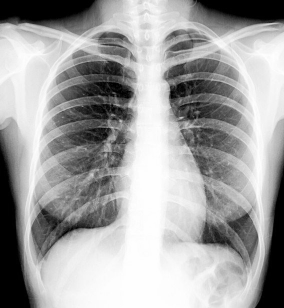
(a) Chest X-Ray

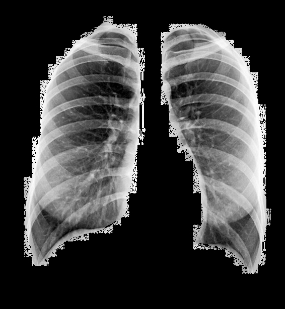
(b) Portion for Lungs

(c) Prediction

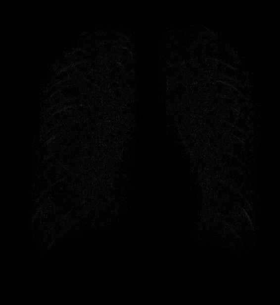
(d) Difference

Figure 3: Simple FPCA analysis with the prediction and the difference between the observed and predicted values for the lung region.

Our purpose was to reduce the dimensionality of the arbitrary shaped region composed by pixels of lungs. Because the original image did not contain any missing values, it was not a missing data problem. It was inappropriate to include any pixels outside the lungs in dimension reduction because they did not belong to our interest. We removed these pixels from the chest X-ray image and obtained an image for the lungs only (Fgure 3(b)). Because the RGB values were all identical, it was enough to analyze the information contained by one of the channels. The size of the chest X-ray image was $615\times 556$. The number of the pixels contained by the lungs was $154,\!835$, about $44.5\%$ of the total number of pixels. We assumed that the distribution given by (2) was normal. We implemented the simple FPCA model with the loglikelihood function given by (6) to the lung region. We used BIC to estimate $k$ and obtained $\hat{k}_{BIC}=38$. We then used $k=38$ to derive the final decomposition. It was used to to recover the image for the lung region only (Figure 3(c)). We found that it was close to the original image. We confirmed the conclusion by looking at the absolute difference between the recovered image and the original image for the lung region. The result is displayed in Figure 3(d).

To compare, we also tried missMDA and generalizedPCA. Their implementations were terminated by error messages without any outputs. The reason probably was that the two methods were designed for missing data, but the study was not a missing data problem. Only our proposed method could be used to this case. It successfully reduced the dimensionality for the irregular shaped region composed by the lungs only.

4.3 Dimension Reduction for Count

We applied our method to the country-level daily confirmed COVID-19 data set. The COVID-19 data are reported by the World Health Organized (WHO) from the beginning of the outbreak of COVID-19 (i.e., January 22, 2020) to now (i.e., August 2 2021). The data set contains the numbers of daily new confirmed cases, deaths, and recoveries, given by countries. Because all of the variables are count, a count data set is composed by using the numbers of daily new confirmed cases, deaths or recoveries. Because our interest was the confirmed cases, we excluded deaths and recoveries in the analysis.

Note that FPCA can be implemented to any kinds of exponential family distributions beyond normal. All $x_{ij}$ were count in this implementation and the distribution given by (2) represented PMFs for count random variables. We were not able to use traditional PCA or missMDA because they are developed for normally distributed random variables. Therefore, we only need to compare our method with generalizedPCA.

It is well known that the outbreak of COVID-19 has become a worldwide ongoing pandemic since March 2020. The first patient of COVID-19 appeared in Wuhan, China, on December 1 2019. In late December, a cluster of pneumonia cases of unknown cause was reported by local health authorities in Wuhan with clinical presentations greatly resembling viral pneumonia [5, 35]. Deep sequencing analysis from lower respiratory tract samples indicated a novel coronavirus [15, 20]. The virus of COVID-19 primarily spreads between people via respiratory droplets from breathing, coughing, and sneezing, which can cause cluster infections in society. To avoid cluster infections, many countries have imposed travel restrictions in Spring 2020 [42]. According to the website of WHO, until August 2 2021, the outbreak has affected over 200 countries and territories with more than $200$ million confirmed cases and $4$ million deaths in the entire world. The most serious country is the United States. It has over $36$ million confirmed cases and $632$ thousand deaths.

Figure 4: PCs in simple FPCA model by assuming that observations follows the quasi-Poisson distribution.

We naturally constructed a matrix for count by taking $x_{ij}$ as the number of new confirmed cases with $i$ representing for countries and $j$ for dates. To account for overdispersion, we assumed that $x_{ij}$ followed the quasi-Poisson distribution with dispersion parameter $\phi$. In particular, we assumed that $x_{ij}|\xi_{ij}\sim{\cal P}(\mu_{ij}\xi_{ij})$, where $\xi_{ij}\sim\Gamma(\mu_{ij}/(\phi-1),\mu_{ij}/(\phi-1))$ were independent random effects, such that we had ${\rm E}(x_{ij})=\mu_{ij}$ and ${\rm V}(x_{ij})=\phi\mu_{ij}$. We modeled $\mu_{ij}$ by (3) with $\gamma_{ij}=0$ for all $i$ and $j$, implying that it was the simple FPCA model.

The data were sparse at the beginning of the outbreak. Many low populated countries reported zeros in many days during the outbreak period. We removed these countries in our analysis. Because China was special, we did not put it in the data. The final data set had $110$ countries and $459$ days. We coded the countries by the decreasing order based on numbers of country-level cumulative confirmed cases until August 2 2021. It covered the period from May 1 2020 to August 2 2021 with many high populated countries, such as the United States (the first country), India (the second country), Brazil (the third country), and etc. The data set contained over $99\%$ of the total number of confirmed cases in the period with more than $90\%$ of the total population in the world (not including China). We estimated $k$ by BIC in the quasi-Poisson model and obtained $\hat{k}_{BIC}=9$. According to the deviance goodness-of-fit statistic measure ($G^{2}$), the model accounted for over $98.5\%$ of the total $G^{2}$ values. We used $k=9$ in (6) and obtained the simple FPCA decomposition. We used it to derive the PCs (Figure 4) and the loadings (Figure 5).

Figure 5: Loadings in simple FPCA model by assuming that observations follows the quasi-Poisson distribution.

Our result indicated that the first PC accounted for $82.2\%$ total $G^{2}$ values. It reflected the overall temporal trend of the entire world. It showed that the total number of confirmed cases would increased fast in Fall 2021. Based on the first loading, we claimed that this would occur in the United States, India, and many European countries. The second PC accounted for $7.85\%$ total $G^{2}$ values. It contained a decreasing trend in Spring 2020 and 2021 and an increasing trend in Fall 2020. Starting from July 1 2021, the trend became increased with a higher rate than that in Fall 2020, indicating that the outbreak would be more serious in Fall 2021. This trend was also confirmed by the third PCs which account for $3.68\%$ total $G^{2}$ values. The findings based on the first three PCs were consistent. Based on the trends in Fall 2020, we predicted that the number of daily new confirmed cases would be kept at higher level until the end of 2021. The situation would not change until the beginning of 2022.

We interpreted the first loading by the overall severity of the countries. The pattern was consistent with the over severity of the countries. The vague patterns appeared from the second to the ninth loadings indicated that the infections in different countries were highly correlated with each other. The infections are word-wide. It is impossible to terminate the spread of COVID-19 by countries individually.

To compare, we also implemented generalizedPCA to the data. Based on the predicted values, we computed its $G^{2}$ values. Our result showed that generalizedPCA interpreted less $G^{2}$ values than our method. For instance, if $k=2$, then generalizedPCA interpreted about $80\%$ but our simple FPCA interpreted about $90\%$. If $k=9$, then generalizedPCA interpreted about $93.4\%$ but our simple FPCA about $98.8\%$. Therefore, our method better interpreted the overall trends in the numbers of new confirmed cases of COVID-19 than generalizedPCA.

5 Discussion

In this article, we propose a new dimension reduction method called flexible PCA (FPCA) by extensions of previous PCA models for matrices. An obvious advantage is that our method can be implemented to exponential family distributions in arbitrary shaped regions but traditional PCA can only be implemented to normal distributions in matrices. The research problem investigated by our method is different from that investigated by previous PCA methods for missing values, because we purposely remove observations outside of the region of interest in the analysis even though they are observed. Therefore, missing data mechanism is not an issue in FPCA, but it is an issue in previous PCA methods for missing data. As SVD is a matrix technique, any PCA methods with SVD cannot be implemented to the problem studied by the article. To overcome the difficulty, we propose statistical models with the maximum likelihood approach in the derivation.

The finding of the article indicates that the usage of statistical models is important in extending matrix-based statistical and machine learning techniques, not limited to traditional PCA for matrices. Matrix data are well-structured and well-organized. Due to rapid development of computer technologies, unstructured or unorganized data are often collected in routine date collection procedures, leading to an important task to extend previous methods, such that they can be used to analyze this kind of data. Our research indicates that statistical models are important in the extensions. Therefore, the impact of the research is not limited to PCA. We believe our idea can also be migrated to other well-known matrix-based methods, such as canonical correlation analysis and factor analysis. This is left to future research.

References

- [1] Anderson, T. (2003). An Introduction to Multivariate Statistical Analysis. Wiley, New York, USA.
- [2] Bai, Z., Chio, K.P., and Fujikoshi, Y. (2018). Consistency of AIC and BIC in estimating the number of significant components in high-dimensional principal component analysis. Annals of Statistics, 46, 1050-1076.
- [3] Carroll, J.D. and Chang, J.J. (1970). Analysis of individual differences in multidimensional scaling via an N-way generalization of “Eckart-Young” decomposition. Psychometrika, 35 283-319.
- [4] Celik, T. (2009). Unsupervised change detection in satellite images using principal component analysis and -means clustering. IEEE Geoscience and Remote Sensing Letters, 6, Article 4.
- [5] Chen, N., Zhou, M., Dong, X., Qu, J., Gong, F., Han, Y., Qiu, Y., Wang, J., Liu, Y., Wei, Y., Xia, J., Yu, T., Zhang, X., and Zhang, L. (2020). Epidemiological and clinical characteristics of 99 cases of 2019 novel coronavirus pneumonia in Wuhan, China: a descriptive study. The Lancet, 395, 507-513.
- [6] Choi, S.W., Park, J.H., Lee, I.B. (2004). Process monitoring using a Gaussian mixture model via principal component analysis and discriminant analysis. Computer and Chemical Engineering, 28, 1377-1387.
- [7] Collins, M., DasGupta, S., and Schapire, R.E. (2001). A generalization of principal component analysis to the exponential family. In Advances in Neural Information Processing Systems, 14, eds. Dieterich, T., Becker, S., and Ghahramani, Z., Cambridge, MA: MIT PRess, pp: 617-624.
- [8] Cook, R.D., and Nachtsheim, C.J. (1994). Re-weighting to archive elliptically contoured covariates in regression. Journal of the American Statistical Association, 89, 592-599.
- [9] Cook, D. and Ni, L. (2005). Sufficient dimension reduction via inverse regression: a minimum discrepancy approach. Journal of the American Statistical Association, 100, 410-428.
- [10] Cook, D. (2007). Fisher Lecture: dimension reduction in regression. Statistical Science, 22, 1-26.
- [11] Demsar, U., P. Harris, C. Brunsdon, A. S. Fotheringham, and S. McLoone. (2013). Principal components analysis on spatial data: an Overview. Annals of the Association of American Geographers 103, 106-128.
- [12] Donoho, D., and Jin, J. (2004). Higher criticism for detecting sparse heterogeneous mixtures. Annals of Statistics, 32, 962-994.
- [13] Dray, S., and Josse, J. (2015). Principal component analysis with missing values: a comparative survey of methods. Plant Ecology, 216, 657-667.
- [14] Fan, J., Guo, S., and Hao, N. (2012). Variance estimation using refitted cross-validation in ultrahigh dimensional regression. Journal of Royal Statistical Society Series B, 74, 37-55.
- [15] Feng, Z. (2020). Urgent research agenda for the novel coronavirus epidemic: transmission and non-pharmaceutical mitigation strategies. Chinese Journal of Epidemiology, 41, 135-138.
- [16] Ferguson, T.S. (1996). A Course in Large Sample Theory, Chapman & Hall/CRC Press, Boca Raton, Florida.
- [17] Gabriel, K.R. (1998). Generalised bilinear regression. Biometrika, 85, 689-700.
- [18] Gardner, J.W. (1991). Detection of vapours and odours from a multisensor array using pattern recognition Part I. principal component and cluster analysis. Sensors and actuators B, 4, 109-11.
- [19] Hoff, P.D. (2005). Bilinear mixed-effects models for dyadic data. Journal of the American Statistical Association, 100, 286-295.
- [20] Huang, C., Wang, Y., Li, X., Ren, L., Zhao, J., Hu., Y., Zhang, L., Fan, G., Xu, J., Gu., X., Cheng, Z., Yu, T., Xia, J., Wei, Y., Wu., W., Xie, X., Yin, W., Li, H., Liu, M., Xiao, Y., Gao, H., Guo, L., Xie, J., Wang, G., Jiang, R., Gao, Z., Jin, Q., Wang, J., Cao, B. (2020). Clinical features of patients infected with 2019 novel coronavirus in Wuhan, China. The Lancet, 395, 497-506.
- [21] Huang, H., Liu, X., Zhang, T., and Yang, B. (2020). Regression PCA for moving objects separation. Proceeding of 2020 IEEE Global Communications Conference (GLOBECOM2020, doi: 10.1109/GLOBECOM42002.2020.9322471.
- [22] Jolliffe, I. (2002). Principal Component Analysis, 2nd Edition. New York: Springer-Verlag.
- [23] Johnstone, I.M. (2001). On the distribution of the largest eigenvalue in principal components analysis. Annals of Statistics, 29, 295-327.
- [24] Josse, J., and Husson, F. (2016). missMDA: a package for handling missing values in multivariate data analysis. Journal of Statistical Software, 17, doi:10.18637/jss.v070.i01.
- [25] Kiers, H. (1997). Weighted least squares fitting using ordinary least squares algorothms. Psychometrika, 62, 251-266.
- [26] Kolda, T.G. and Bader, B.W. (2009). Tensor decompositions and applications. SIAM Reviews, 51, 455-500.
- [27] Landgraf, A.J., and Lee, Y. (2020). Generalized principal component analysis: projection of saturated model parameters. Technometrics, 62, 459-472.
- [28] Lawrence, N. (2005). Probabilistic non-linear principal component analysis with Gaussian process latent variable models. Journal of Machine Learning Research, 6, 1783-1816.
- [29] Li, B. and Wang, S. (2007). On directional regression for dimension reduction. Journal of American Statistical Association, 102, 997-1008.
- [30] Li, K.C., and Duan, N. (1989). Regression analysis under link violation. The Annals of Statistics, 17, 1009-1052.
- [31] Liu, X., Huang, H., Tang, W., Zhang, T., and Yang, B. (2020). Low-rank sparse tensor approximations for large high-resolution videos. 2020 19th IEEE International Conference on Machine Learning and Applications (ICMLA), 65-74, DOI: 10.1109/ICMLA51294.2020.00020
- [32] Marx, B., Smith, E.P. (1990). Principal component estimation for generalized linear regression. Biometrika, 77, 23-31.
- [33] Rubin, D. (1976). Inference and missing data. Biometrika, 63, 581-592.
- [34] Sousa, S.I.V., Matins, F.G., Alvim-Ferraz, M.C.M., Pereira, M.C. (2007). Multiple linear regression and artificial neural networks based on principal components to predict ozone concentrations. Environmental Modelling & Software, 22, 97-103.
- [35] Sun, K., Chen, J., and Viboud, C. (2020). Early epidemiological analysis of the coronavirus disease 2019 outbreak based on crowdsourced data: a population-level observational study. The Lancet Digital Health.
- [36] Tipping, M.E. and Bishop, C.M. (1999). Probabilistic principal component analysis. Journal of Royal Statistical Society Series B, 61, 611-622.
- [37] Tucker, L.R. (1966). Some mathematical notes on three-mode factor analysis. Psychometrika, 31, 279-311.
- [38] Xia, Y., Tong, H., Li, W.K., and Zhu, L.X. (2002). An adaptive estimation of dimension reduction space. Journal of Royal Statistical Society, 64, 363-410.
- [39] Zhang, L., Dong, W., Zhang, D., and Shi, G. (2010). Two-stage image denoising by principal component analysis with local pixel grouping. Pattern Recognition, 43, 1531-1549.
- [40] Zhang, T. and Yang, B. (2016). Big data dimension reduction using PCA. Proceeding of IEEE Smartcloud, article 82, DOI: 10.1109/SmartCloud.2016.33
- [41] Zhang, T. and Yang, B. (2018). Dimension reduction for big data. Statistics and Its Interface, 11, 295-306.
- [42] Zhang, T., and Lin, G. (2021). Generalized -means in GLMs with applications to the outbreak of COVID-19 in the United States. Computational Statistics and Data Analysis, 159, 107217, DOI: 10.1016/j.csda.2021.107217.
- [43] Zhang, Y., Li, R., and Tsai,, C. (2010). Regularization parameter selections via generalized information criterion. Journal of the American Statistical Association, 105, 312-323.
- [44] Zhao, G. and Mactean, A.L. (2000). A comparison of canonical discriminant analysis and principal component analysis for spectral transformation. Photogrammetric engineering & Remote Sensing, 66, 841-847.