Gravitational waves in higher-order $R^{2}$ gravity

Abstract

We perform a comprehensive study of gravitational waves in the context of the higher-order quadratic scalar curvature gravity, which encompasses the ordinary Einstein-Hilbert term in the action plus an $R^{2}$ contribution and a term of the type $R\square R$. The main focus is on gravitational waves emitted by binary systems such as binary black holes and binary pulsars in the approximation of circular orbits and nonrelativistic motion. The waveform of higher-order gravitational waves from binary black holes is constructed and compared with the waveform predicted by standard general relativity; we conclude that the merger occurs earlier in our model than what would be expected from GR. The decreasing rate of the orbital period in binary pulsars is used to constrain the coupling parameters of our higher-order $R^{2}$ gravity; this is done with Hulse-Taylor binary pulsar data leading to $\kappa_{0}^{-1}\lesssim 1.1\times 10^{16}\,\text{m}^{2}$ , where $\kappa_{0}^{-1}$ is the coupling constant for the $R^{2}$ contribution.

I INTRODUCTION

It is hardly necessary to motivate the appropriateness of studying gravitational waves (GWs) in the light of LIGO-VIRGO Collaboration observations, from the discovery event Abbott2016 , to the neutron-star merger detection Abbott2017 inaugurating the multimessenger astronomy, up to the most recent observational results Abbott2019 ; Abbott2021 .

As a matter of fact, the direct detection of GW events confirmed the indirect predictions stemming from the Hulse and Taylor binary pulsar Hulse1975 ; Taylor1982 ; Weisberg2004 : The emission of gravitational waves carries energy and momentum away from the parent binary system, which in turn reduces its orbital period and mass separation, leading to an inspiral motion ending with a coalescence. The importance of the papers mentioned above includes the confirmations of all the predictions of general relativity (GR) on this regard. On the one hand, this fact is rather satisfying for Einstein’s theory of gravity; on the other hand, it imposes serious constraints onto modified theories for gravitational interaction—so much so, that modified gravity frameworks that predict propagation velocities for detectable spin-2 gravitational waves different from the speed of light in vacuum are in difficulty Abbott2019 ; Kase2018 .

Even though gravitational wave observations definitely favor GR as the correct theory of gravity, the physics community knows it cannot be the final theory. The reason for this consensus comes from high-energy regimes, where quantization is specially required. In effect, theoretical contributions going back to the works, e.g., by Stelle Stelle1977 ; Stelle1978 propose the modification of the Einstein-Hilbert action by the inclusion of terms like the square of the curvature scalar, $R^{2}$, and other invariants built from the curvature scalar and its derivatives LeeWick1970 ; Donoghue2019 . In a similar direction, the Starobinsky inflation model uses the $R^{2}$ term Starobinsky1979 ; Gurovich1979 ; Starobinsky1980 to produce one of the strongest realizations of inflationary scenarios—in fact, it predicts a tensor-to-scalar ratio $r$ per scalar tilt $n_{s}$ deep within the confidence contours produced with Plack satellite observations PlanckCollab2018 and BICEP2/Keck plus BAO data BICEP2Collab2018 .

That GR is not the ultimate theory for gravitational interaction is also hinted at from the infrared regime in cosmology. The description of late-time Universe dynamics hinges on the ubiquitous dark energy Huterer2017 ; Motta2021 ; Slozar2019 . It is well known that the simple cosmological constant could serve as a good candidate for describing dark energy and the present-day acceleration of the cosmos. But then again, the very concept of a cosmological constant faces problems, either regarding its physical interpretation Weinberg1989 ; Carroll2001 or related to the challenges against the concordance $\Lambda$CDM model Skara2021 . Indeed, the $H_{0}$ tension, the $\sigma_{8}$ problem and the lensing amplitude $A_{L}$ anomaly Verde2019 ; Valentino2021 ; Efstathiou2021 ; Handley2021 ; Valentino2019 ; Valentino2017 ; Gannouji2018 ; Vagnozzi2019 ; Vagnozzi2021a ; Vagnozzi2021b have galvanized the ongoing “cosmology crisis.” This makes room for alternative theories of gravity Saridakis2021 .

One of the possible avenues of research in the context of modified gravity is to consider higher-order quadratic-curvature scalar models. By higher-order quadratic-curvature scalar gravity, we mean models containing the $R^{2}$ term in the action and also invariants built from derivatives of the curvature scalar, viz. $R\square R$. In actuality, some papers from the 1990s explored such terms Wands1994 in the inflationary context Berkin1990 ; Gottlober1990 ; Gottlober1991 ; Amendola1993 . References JCAP2019 ; Castellanos2018 ; Iihoshi2011 explore an equivalent inflationary model on a deeper level and constrain the coupling constant associated with the higher-order contribution via observational data. Higher-order gravity models of the type $f\left(R,\nabla R,\dots,\nabla^{n}R\right)$ may be cast in their scalar-multitensor equivalent form with some interesting consequences PRD2016 ; PRD2019 .

Usually, the business of constraining modified gravity models is done in the realm of cosmological data Sotiriou2010 ; DeFelice2010 ; Nojiri2011 ; Nojiri2017 ; GERG2015 ; Capozziello2017 , but gravitational wave observations could also contribute to the task on a different scale Berti2015 ; Naf2011 ; DeLaurentis2013 ; Capozziello2009 ; Kuntz2017 . It is with this in mind that we seek to investigate the GW predicted for binary inspirals in the context of a higher-order quadratic-curvature scalar model. Our model contains the terms $R^{2}$ and $R\square R$ alongside the Einstein-Hilbert term in the action integral of the model. We will show that this model, when linearized on a flat background, gives rise to a spin-2 mode of the gravitational waves (consonant to the $h_{\mu\nu}$ predicted within GR) plus two spin-0 modes, $\Phi_{-}$ and $\Phi_{+}$. These two scalar modes are coupled in a nontrivial way, one serving as source for the other. The scalar mode $\Phi_{+}$ associated with the $R\square R$ contribution is treated perturbatively.

Great care is devoted to building the solutions to the linearized field equations in a self-contained way. Accordingly, our paper shows explicitly how to apply the Green’s method to solve the differential equations for the modified gravity model, and how the functional forms of $\Phi_{-}$ in terms of integrals involving Bessel functions are born. In the same spirit, we detail the calculation of the energy-momentum pseudotensor in the higher-order $R^{2}$ model, which involves many more terms than the treatment given by GR. This is potentially useful for other works dealing with models containing higher-order derivatives of the curvature-based scalars. We should point out that other works have approached gravitational waves for models involving the $R^{2}$ term—see, e.g., Refs. Cano2019 ; Berry2011 ; Naf2010 ; Capozziello2011 ; Aguiar2003 . Our contribution is the thorough step-by-step derivation of the results, from the linearized field equation until the final constraining of the associated coupling, besides the inclusion of the term $R\square R$ and the detailed study of its corrections to gravitational wave physics.

Our modified gravitational wave solutions are specified for binary systems, aiming for contact with observations later in the paper. We take the approximation of the nonrelativistic motion of the pair of astrophysical objects in the binary system; a circular orbit is also assumed. The spin-0 mode $\Phi_{-}$ related to the $R^{2}$ contribution is carefully computed in this context; it exhibits two different regimes according to a well-defined scale. In fact, there is a propagating oscillatory regime for $\Phi_{-}$ and a damped regime.

The modified GWs emitted by binary black holes are calculated. Their waveform is compared to the one predicted by GR. It is shown that the rise in the amplitude and frequency of the strain before the chirp is more pronounced in our higher-order model than in GR, although the difference is subtle. This result is qualitatively interesting, but the real constraint to our model comes from its application to the description of gravitational waves emitted by binary pulsars. Incidentally, there is a difference in the treatment of black-hole binaries with respect to neutron-star binaries in our higher-order quadratic-curvature scalar model: the orbital dynamics of the binary system is different in each instance. In any case, we use the binary pulsar investigated by Hulse, Taylor, and Weisberg Hulse1975 ; Taylor1982 ; Weisberg2004 to constrain the coupling constants $\kappa_{0}$ and $\beta_{0}$ associated with the extra terms $R^{2}$ and $R\square R$ in the action. These constraints contribute to the existing ones in the literature Berry2011 ; Naf2011 .

Our conventions follow the ones in Ref. Carroll2004 : i.e., the Minkowski metric is written as $\left(\eta_{\mu\nu}\right)=\text{diag}\left(-1,+1,+1,+1\right)$ in Cartesian coordinates; the Riemann tensor is defined as $R_{\,\sigma\mu\nu}^{\rho}=\partial_{\mu}\Gamma_{\,\nu\sigma}^{\rho}-\partial_{\nu}\Gamma_{\,\mu\sigma}^{\rho}+\Gamma_{\,\mu\lambda}^{\rho}\Gamma_{\,\nu\sigma}^{\lambda}-\Gamma_{\,\nu\lambda}^{\rho}\Gamma_{\,\mu\sigma}^{\lambda}$ ; and, the Ricci tensor is given by the contraction $R_{\mu\nu}=R_{\,\mu\rho\nu}^{\rho}$.

The structure of the paper is as follows: In Sec. II, the action integral for the higher-order $R^{2}$ model is presented, the equations of motion are written, and the weak-field regime of those equations is carried out. Even in the linearized form, the field equations are complex enough to demand a method of order deduction for enabling their solution; this method is laid down in Sec. III and is based on a scalar-tensor decomposition of the metric tensor. Section IV presents the solutions to the field equations and their multipole expansion; the expressions are given in terms of the energy-momentum tensor of the source. In Sec. V, the form of the energy-momentum tensor is particularized to the case of a binary system, the closed functional forms for the gravitational waves are determined, and the expression for the power radiated in the form of GWs is computed under the assumption of a circular orbit approximation. Section VI is devoted to the study of binary black holes: the focus is to determine how the additional terms in our modified gravity model alter the waveform of the gravitational wave. Binary pulsar inspirals are studied in Sec. VII, where the main objective is to constrain the extra couplings of our higher-order quadratic-curvature scalar model through the observational data coming from the Hulse-Taylor binary pulsar. Our final comments are given in Sec. VIII.

II HIGHER-ORDER $R^{2}$ GRAVITY IN THE WEAK-FIELD REGIME

We begin by stating the action of our model:

$$S=\frac{1}{c}\frac{1}{2\chi}\int d^{4}x\sqrt{-g}\left[R+\frac{1}{2\kappa_{0}}R^{2}-\frac{\beta_{0}}{2\kappa_{0}^{2}}R\square R+\mathcal{L}_{m}\right]\qquad\left(\chi=\frac{8\pi G}{c^{4}}=\frac{1}{M_{P}^{2}}\right)\,.$$ (1)

We call quadratic-curvature scalar the contribution from the term scaling with $R^{2}$. The higher-order contribution corresponds to the $R\square R$ term. (The D’Alembertian operator $\square\equiv g^{\mu\nu}\nabla_{\mu}\nabla_{\nu}$ is given in terms of the covariant derivative $\nabla_{\mu}$ contraction.) The coupling constant of the higher-order term is written as $\left(\beta_{0}/2\kappa_{0}^{2}\right)$ so that $\beta_{0}$ is a dimensionless constant. The coupling $\kappa_{0}$ has the dimension of $\left(\text{length}\right){}^{-2}$. Notice that the Einstein-Hilbert action is recovered in the limit of a large $\kappa_{0}$ and a small $\beta_{0}$.

The equation of motion is obtained from Eq. (1) by varying with respect to $g^{\mu\nu}$:

$$G_{\mu\nu}+\frac{1}{2\kappa_{0}}H_{\mu\nu}+\frac{\beta_{0}}{2\kappa_{0}^{2}}I_{\mu\nu}=\chi T_{\mu\nu}\,,$$ (2)

where

$$G_{\mu\nu}=R_{\mu\nu}-\frac{1}{2}g_{\mu\nu}R$$ (3)

is the standard Einstein tensor Aguiar2003 ,

$$H_{\mu\nu}\equiv R\left(R_{\mu\nu}+G_{\mu\nu}\right)-2\left(\nabla_{\nu}\nabla_{\mu}R-g_{\mu\nu}\square R\right)$$ (4)

is the contribution coming from the $R^{2}$ term, and AstroSpScien2011

$$I_{\mu\nu}\equiv\nabla_{\mu}R\nabla_{\nu}R-2R_{\mu\nu}\square R-\frac{1}{2}g_{\mu\nu}\nabla_{\rho}R\nabla^{\rho}R+2\left(\nabla_{\nu}\nabla_{\mu}\square R-2g_{\mu\nu}\square^{2}R\right)$$ (5)

stems from the higher-order term.

In the following, we work out the weak-field approximation of the above field equation in a Minkowski background. The metric tensor will be written as

$$g_{\mu\nu}=\eta_{\mu\nu}+h_{\mu\nu}\,,$$ (6)

with $\left|h_{\mu\nu}\right|\ll 1$ so that the linear approximations hold. Then, $g^{\mu\nu}=\eta^{\mu\nu}-h^{\mu\nu}$ and $h=\eta^{\mu\nu}h_{\mu\nu}$. It pays off to introduce the definition of the the trace-reverse tensor:

$$\bar{h}_{\mu\nu}=h_{\mu\nu}-\frac{1}{2}\eta_{\mu\nu}h\,,$$ (7)

in terms of which Eq. (3) reads

$$G_{\mu\nu}=-\frac{1}{2}\left\{\eta^{\rho\sigma}\partial_{\rho}\partial_{\sigma}\bar{h}_{\mu\nu}+\left[\eta_{\mu\nu}\partial_{\rho}\left(\partial_{\sigma}\bar{h}^{\rho\sigma}\right)-\partial_{\mu}\left(\partial^{\rho}\bar{h}_{\nu\rho}\right)-\partial_{\nu}\left(\partial^{\rho}\bar{h}_{\mu\rho}\right)\right]\right\}\,.$$ (8)

The $R^{2}$-term contribution $H_{\mu\nu}$ in the weak-field regime is

$$H_{\mu\nu}=-2\left[\partial_{\nu}\partial_{\mu}-\eta_{\mu\nu}\eta^{\rho\sigma}\partial_{\rho}\partial_{\sigma}\right]R\,,$$ (9)

where $R$ is now expressed in terms of the trace-reverse tensor:

$$R=\partial_{\alpha}\partial_{\beta}\bar{h}^{\alpha\beta}+\frac{1}{2}\eta^{\alpha\beta}\partial_{\alpha}\partial_{\beta}\bar{h}\,.$$ (10)

This quantity also appears in the contribution $I_{\mu\nu}$ from the $R\square R$ term in the weak-field regime:

$$I_{\mu\nu}=2\left[\partial_{\nu}\partial_{\mu}-2\eta_{\mu\nu}\left(\eta^{\lambda\tau}\partial_{\lambda}\partial_{\tau}\right)\right]\left(\eta^{\rho\sigma}\partial_{\rho}\partial_{\sigma}R\right)\,.$$ (11)

We are now in a position to write down the entire field equation (2) in the weak-field approximation by using the results (8), (9), and (11) for $G_{\mu\nu}$, $H_{\mu\nu}$, and $I_{\mu\nu}$, respectively. In fact,

$$\square\bar{h}_{\mu\nu}+\left[\eta_{\mu\nu}\partial_{\rho}\partial_{\sigma}\bar{h}^{\rho\sigma}-\partial_{\mu}\partial^{\rho}\bar{h}_{\nu\rho}-\partial_{\nu}\partial^{\rho}\bar{h}_{\mu\rho}\right]$$

$$+\frac{2}{\kappa_{0}}\left(\partial_{\mu}\partial_{\nu}-\eta_{\mu\nu}\square\right)\left[\partial^{\rho}\partial^{\sigma}\left(\bar{h}_{\rho\sigma}+\frac{1}{2}\eta_{\rho\sigma}\bar{h}\right)\right]$$

$$-\frac{2\beta_{0}}{\kappa_{0}^{2}}\left(\partial_{\mu}\partial_{\nu}-\eta_{\mu\nu}\square\right)\left[\square\partial^{\rho}\partial^{\sigma}\left(\bar{h}_{\rho\sigma}+\frac{1}{2}\eta_{\rho\sigma}\bar{h}\right)\right] =-2\chi T_{\mu\nu}\,,$$ (12)

where the first and second terms on the lhs are those obtained in standard GR, the third term comes from the $R^{2}$ contribution to the action, and the fourth term is born from the higher-order term $R\square R$. (In the weak-field regime, it turns out that $\square=\eta^{\rho\sigma}\partial_{\rho}\partial_{\sigma}$.)

The field equation in the weak-field approximation is considerably simplified in GR when one uses the harmonic gauge fixing condition, $\partial_{\nu}\bar{h}^{\mu\nu}=0$. This is very satisfying, because it eliminates the last three terms in the first line of the field equation (12), and we are left with $\boxempty\bar{h}_{\mu\nu}=-2\chi T_{\mu\nu}$. However, the harmonic gauge on $\bar{h}^{\mu\nu}$ might not be useful or even attainable in higher-order gravity Berry2011 . So, we should study the gauge fixing in higher-order gravity with greater care. This will be dealt with in the next section.

For the time being, we take the trace of the linearized field equation:

$$\square\bar{h}+2\partial^{\nu}\partial^{\rho}\bar{h}_{\nu\rho}-\frac{6}{\kappa_{0}}\square\left[\partial^{\rho}\partial^{\sigma}\left(\bar{h}_{\rho\sigma}+\frac{1}{2}\eta_{\rho\sigma}\bar{h}\right)\right]+\frac{6\beta_{0}}{\kappa_{0}^{2}}\square\left[\square\partial^{\rho}\partial^{\sigma}\left(\bar{h}_{\rho\sigma}+\frac{1}{2}\eta_{\rho\sigma}\bar{h}\right)\right]=-2\chi T\,.$$ (13)

The solutions to the sixth-order differential equation (12) will be found after decomposing the trace-reverse tensor $\bar{h}_{\mu\nu}$ into a scalar part and a tensorial sector.

III SCALAR-TENSOR DECOMPOSITION IN THE WEAK-FIELD REGIME AND THE MODIFIED HARMONIC GAUGE

We define a new dimensionless scalar field $\Phi$ proportional to the curvature scalar $R$:

$$\kappa_{0}\Phi\equiv R=\partial^{\mu}\partial^{\nu}\left(\bar{h}_{\mu\nu}+\frac{1}{2}\eta_{\mu\nu}\bar{h}\right)\,,$$ (14)

and we decompose the linearized metric into a form depending on both $\Phi$ and $\square\Phi$:

$$\bar{h}_{\mu\nu}=\tilde{h}_{\mu\nu}+\eta_{\mu\nu}\left(\Phi-\frac{\beta_{0}}{\kappa_{0}}\square\Phi\right)\,,$$ (15)

so that the trace is

$$\bar{h}=\tilde{h}+4\left(\Phi-\frac{\beta_{0}}{\kappa_{0}}\square\Phi\right)\,.$$ (16)

Our trace-reverse tensor decomposition proposal [Eq. (15)] was inspired by the content in Ref. Accioly2016 .

We choose a gauge condition such that

$$\partial_{\mu}\bar{h}^{\mu\nu}=\partial^{\nu}\left(\Phi-\frac{\beta_{0}}{\kappa_{0}}\square\Phi\right)\,,$$

which leads to the harmonic gauge on $\tilde{h}^{\mu\nu}$:

$$\partial_{\mu}\tilde{h}^{\mu\nu}=0\qquad\left(\text{harmonic gauge}\right)\,.$$ (17)

Using Eqs. (15), (16), and (17), the linearized field equation (12) reads

$$\square\tilde{h}_{\mu\nu}=-2\chi T_{\mu\nu},$$ (18)

and the trace of the linearized field equation (13) reduces to

$$\frac{\beta_{0}}{\kappa_{0}^{2}}\square^{2}\Phi-\frac{1}{\kappa_{0}}\square\Phi+\frac{1}{3}\Phi=-\frac{\chi}{3\kappa_{0}}T\,.$$ (19)

This is a fourth-order differential equation and, as such, is a delicate matter to deal with. We will reduce its order below.

We claim that Eq. (19) can the cast into the form

$$\left(\frac{\square}{\kappa_{0}}-K_{-}\right)\left(\beta_{0}\frac{\square}{\kappa_{0}}-K_{+}\right)\Phi=-\frac{\chi}{3\kappa_{0}}T\,.$$ (20)

In order to determine the constants $K_{\pm}$ that allow for this possibility, we open up the above expression and compare with Eq. (19). The result is

$$K_{-} =\frac{1}{2\beta_{0}}\left[1-\sqrt{1-\frac{4}{3}\beta_{0}}\right]\,,$$ (21)

$$K_{+} =\frac{1}{2}\left[1+\sqrt{1-\frac{4}{3}\beta_{0}}\right].$$ (22)

Let us further define

$$\Phi\equiv\Phi_{+}\,,$$ (23)

and, motivated by a sector on the lhs of Eq. (20), the new field

$$\left(\beta_{0}\frac{\square}{\kappa_{0}}-K_{+}\right)\Phi_{+}\equiv\Phi_{-}\,.$$ (24)

Equation (20) is then written as

$$\left(\frac{\square}{\kappa_{0}}-K_{-}\right)\Phi_{-}=-\frac{\chi}{3\kappa_{0}}T\,.$$ (25)

Now, Eqs. (24), and (25) may be written in a more compelling form:

$$\left(\square-m_{+}^{2}\right)\Phi_{+}=\frac{\kappa_{0}}{\beta_{0}}\Phi_{-}\,,$$ (26)

and

$$\left(\square-m_{-}^{2}\right)\Phi_{-}=-\frac{\chi}{3}T\,,$$ (27)

where

$$m_{\pm}^{2}=\frac{\kappa_{0}}{2\beta_{0}}\left[1\pm\sqrt{1-\frac{4}{3}\beta_{0}}\right].$$ (28)

Notice that $\left[m_{\pm}^{2}\right]=\left(\text{length}\right)^{-2}$; these parameters could be interpreted as masses of the fields $\Phi_{\pm}$. The original differential equation (19) was thus reduced from a fourth-order equation to a pair of second-order differential equations, viz. Equations (26) and (27).

By using the definitions of the new scalar fields $\Phi_{\pm}$ in Eq. (15) for $\bar{h}_{\mu\nu}$, we conclude that the spacetime wiggles are given by

$$\bar{h}_{\mu\nu}=\tilde{h}_{\mu\nu}+\eta_{\mu\nu}\left[\frac{\beta_{0}}{\kappa_{0}}m_{-}^{2}\Phi_{+}-\Phi_{-}\right]\,.$$ (29)

This is the scalar-tensor decomposition of the gravitational waves in our higher-order $R^{2}$ gravity.

The script to determine the scalar degree of freedom $\Phi$ in our model—see Eq. (14)—is the following: Given the source type characterized by $T$, the first step is to integrate Eq. (27) and find $\Phi_{-}$. The next step is to use $\Phi_{-}$ as the source of $\Phi_{+}$, which is computed through Eq. (26). The field $\Phi_{-}$ is determined univocally given the adequate boundary conditions (such as the requirement for a radiative solution); $\Phi_{+}$ is then also determined univocally in terms of $\Phi_{-}$, as will be explicitly shown in Sec. IV.2. The conclusion is that there is a single scalar degree of freedom corresponding to $\Phi$; the higher-order quadratic scalar curvature model exhibits three degrees of freedom total: two encapsulated in $\tilde{h}_{\mu\nu}$, and one embodied by $\Phi$.

Remark: $R^{2}$ gravity limit.—If $\beta_{0}\ll 1$, the mass parameters $m_{\pm}$ in Eq. (28) reduce to

$$m_{+}^{2}\approx\frac{\kappa_{0}}{\beta_{0}}\left(1-\frac{1}{3}\beta_{0}\right)\text{ \ and \ }m_{-}^{2}\approx\frac{\kappa_{0}}{3}\left(1+\frac{1}{3}\beta_{0}\right)\,.$$ (30)

Therefore, in the limit as $\beta_{0}\rightarrow 0$, the decomposed field equations (24) and (27) simplify to

$$\left(\square-\frac{\kappa_{0}}{3}\right)\Phi_{-}=-\frac{\chi}{3}T\text{ \ and \ }\left(\frac{\beta_{0}}{\kappa_{0}}\square-1\right)\Phi_{+}=\Phi_{-}\Rightarrow\Phi=\Phi_{+}\simeq-\Phi_{-}\,.$$

This leads to the structure

$$\left(\square-\frac{\kappa_{0}}{3}\right)\Phi=\frac{\chi}{3}T\text{ }\,,$$

which is typical of a pure $R^{2}$-gravity model Berry2011 . $\blacksquare$

In the next section, we work on determining solutions to the field equations (18), (26), and (27) in order to characterize the gravitational waves $\bar{h}_{\mu\nu}$.

IV SOLUTIONS TO THE LINEARIZED FIELD EQUATIONS

IV.1 The sourceless equations

The sourceless version of Eq. (18) is solved by $\tilde{h}_{\mu\nu}=\epsilon_{\mu\nu}e^{iq_{\rho}x^{\rho}}+\epsilon_{\mu\nu}^{*}e^{-iq_{\rho}x^{\rho}}$. This is the plane wave solution, $\tilde{h}_{\mu\nu}$ is a massless spin-2 field, and the dispersion relation is

$$\left|\mathbf{q}\right|=\frac{\omega}{c}\,,$$ (31)

where $q^{0}=\omega/c$ and $\mathbf{q}=\left(q^{i}\right)$.

By setting $T=0$ in Eq. (27), we get a differential equation whose solution is $\Phi_{-}=\phi_{-}e^{ik_{\mu}x^{\mu}}+\phi_{-}^{*}e^{-ik_{\mu}x^{\mu}}$, where

$$\left|\mathbf{k}\right|=\sqrt{\frac{\omega^{2}}{c^{2}}-m_{-}^{2}}\,,$$ (32)

with $k^{0}=\omega/c$ and $\mathbf{k}=\left(k^{i}\right)$. Then, we are faced with two different possibilities:

• $\omega\geqslant m_{-}c$. In this case, $\mathbf{k}$ is a real number, the arguments of the exponentials in $\Phi_{-}$ are complex, and the solution is oscillatory.

• $\omega<m_{-}c$. Here, $\mathbf{k}$ is a complex number, the arguments of the exponentials in $\Phi_{-}$ are real, and the solution is either decreasing (damped) or increasing with $x^{\mu}$. The increasing solution blows up as $x\rightarrow\infty$ and should be neglected as unphysical.

The $\Phi_{+}$ field equation does not have a sourceless version: $\Phi_{-}$ is the very source of $\Phi_{+}$, as indicated by Eq. (26).

IV.2 The complete field equations

In the presence of a source, Eq. (18) is solved by

$$\tilde{h}_{\mu\nu}=\frac{4G}{c^{4}}\int d^{3}x^{\prime}\frac{1}{\left|\mathbf{x}-\mathbf{x}^{\prime}\right|}T_{\mu\nu}\left(t_{r},\mathbf{x}^{\prime}\right)\,,$$ (33)

where $t_{r}=t-\left|\mathbf{x}-\mathbf{x}^{\prime}\right|/c$ is the retarded time, and the vector $\mathbf{x}$ (the vector $\mathbf{x}^{\prime}$) points from the origin of the coordinate system to the observer (to the source). Equation (33) is obtained through the retarded Green’s function. This is standard in GR Sabbata1985 ; Carroll2004 , except that in our case, $\tilde{h}_{\mu\nu}$ appears instead of $\bar{h}_{\mu\nu}$.

The formal solution of Eq. (27) for $\Phi_{-}$ is in terms of the Green’s function $G_{\Phi}\left(x^{\mu};x^{\prime\mu}\right)$:

$$\Phi_{-}\left(x^{\mu}\right)=-\frac{\chi}{3}\int G_{\Phi}\left(x^{\mu};x^{\prime\mu}\right)T\left(x^{\prime\mu}\right)d^{4}x^{\prime}\,.$$ (34)

Following the detailed procedure in Appendix A, the explicit form of the retarded Green’s function is [see Eq. (152)]

$$G_{\Phi}\left(x^{\nu};x^{\prime\nu}\right)=-\frac{1}{4\pi}\frac{1}{c}\frac{1}{s}\delta\left(\tau-\frac{s}{c}\right)+\frac{1}{4\pi}\Theta\left(\tau-\frac{s}{c}\right)\frac{1}{c}\frac{m_{-}}{\sqrt{\tau^{2}-\left(\frac{s}{c}\right)^{2}}}J_{1}\left(m_{-}c\sqrt{\tau^{2}-\left(\frac{s}{c}\right)^{2}}\right)\,,$$ (35)

where $\Theta\left(\xi\right)$ is the Heaviside step function, $\tau=\left(t-t^{\prime}\right)$, and $s=\left|\mathbf{s}\right|=\left|\mathbf{x}-\mathbf{x}^{\prime}\right|$. $J_{1}$ is the Bessel function of the first kind. Plugging Eq. (35) into Eq. (34) and manipulating with respect to $t^{\prime}$ leads to Naf2011

$$\Phi_{-}\left(\mathbf{x},t\right)=\frac{2}{3}\frac{G}{c^{4}}\int\frac{1}{s}T\left(\mathbf{x}^{\prime},t_{r}\right)d^{3}\mathbf{x}^{\prime}-m_{-}\frac{2}{3}\frac{G}{c^{4}}\int d^{3}\mathbf{x}^{\prime}\int_{\frac{s}{c}}^{\infty}\frac{J_{1}\left(m_{-}c\sqrt{\tau^{2}-\left(\frac{s}{c}\right)^{2}}\right)}{\sqrt{\tau^{2}-\left(\frac{s}{c}\right)^{2}}}T\left(\mathbf{x}^{\prime},t-\tau\right)d\tau\,.$$ (36)

This equation appears in Ref. Cano2019 in the limit of great distances from the source, where $s\simeq\left|\mathbf{x}\right|$.

Remark: The limits $m_{-}\rightarrow\infty$ and $m_{-}\rightarrow 0$.— Let us comment on the form of Eq. (36) in relation to the possible limits of the mass parameter $m_{-}$. For that, we note that the change of variable $\xi=m_{-}c\sqrt{2\frac{s}{c}\left(\tau-\frac{s}{c}\right)}$ recasts $\Phi_{-}$ into the form

$$\Phi_{-}\left(\mathbf{x},t\right)= \frac{2}{3}\frac{G}{c^{4}}\int\frac{1}{s}T\left(\mathbf{x}^{\prime},t_{r}\right)d^{3}\mathbf{x}^{\prime}$$

$$-\frac{2}{3}\frac{G}{c^{4}}\int d^{3}\mathbf{x}^{\prime}\int_{0}^{\infty}\frac{J_{1}\left(\xi\sqrt{1+\left(\frac{\xi}{2m_{-}s}\right)^{2}}\right)}{s\sqrt{1+\left(\frac{\xi}{2m_{-}s}\right)^{2}}}T\left(\mathbf{x}^{\prime},t_{r}-2\frac{s}{c}\left(\frac{\xi}{2m_{-}s}\right)^{2}\right)d\xi\,.$$

In the limit $m_{-}\rightarrow\infty$, this reduces to

$$\Phi_{-}\left(\mathbf{x},t\right)\approx\frac{2}{3}\frac{G}{c^{4}}\int\frac{1}{s}T\left(\mathbf{x}^{\prime},t_{r}\right)d^{3}\mathbf{x}^{\prime}-\frac{2}{3}\frac{G}{c^{4}}\int\frac{1}{s}T\left(\mathbf{x}^{\prime},t_{r}\right)d^{3}\mathbf{x}^{\prime}\int_{0}^{\infty}J_{1}\left(\xi\right)d\xi=0\qquad\left(m_{-}\rightarrow\infty\right)\,,$$ (37)

because $\int_{0}^{\infty}J_{1}\left(\xi\right)d\xi=1$. This was expected: $m_{-}\rightarrow\infty$ amounts to taking $\kappa_{0}\rightarrow\infty$. This means that the quadratic-curvature scalar term $\propto\kappa_{0}^{-1}R^{2}$ vanishes from the action, and we are left with the standard GR case. This is the same as stating that the scalar mode vanishes.

On the other hand, for $m_{-}=0$, Eq. (36) reduces to

$$\Phi_{-}\left(\mathbf{x},t\right)=\frac{2}{3}\frac{G}{c^{4}}\int\frac{1}{\left|\mathbf{x}-\mathbf{x}^{\prime}\right|}T\left(\mathbf{x}^{\prime},t_{r}\right)d^{3}\mathbf{x}^{\prime}\qquad\left(m_{-}=0\right)\,.$$ (38)

In this way, we see that the scalar mode loses its contribution from the mass and exhibits a similar behavior to the massless spin-2 mode of GR. $\blacksquare$

The form of the differential equation for $\Phi_{+}$ [Eq. (26)] is the same as the one for $\Phi_{-}$ [Eq. (27)]: it suffices to perform the mapping $\Phi_{-}\mapsto\Phi_{+}$, $m_{-}\mapsto m_{+}$, and $\left(-\chi/3\right)T\mapsto\left(\kappa_{0}/\beta_{0}\right)\Phi_{-}$ to obtain the former from the later. Therefore, the solution to Eq. (26) should be formally the same as the solution to Eq. (27). In fact,

$$\Phi_{+}\left(\mathbf{r},t\right)= -\frac{1}{4\pi}\frac{\kappa_{0}}{\beta_{0}}\int\frac{1}{s}\Phi_{-}\left(\mathbf{x}^{\prime},t_{r}\right)d^{3}\mathbf{x}^{\prime}$$

$$+\frac{m_{+}}{4\pi}\frac{\kappa_{0}}{\beta_{0}}\int d^{3}\mathbf{x}^{\prime}\int_{\frac{s}{c}}^{\infty}\frac{J_{1}\left(m_{+}c\sqrt{\tau^{2}-\left(\frac{s}{c}\right)^{2}}\right)}{\sqrt{\tau^{2}-\left(\frac{s}{c}\right)^{2}}}\Phi_{-}\left(\mathbf{x}^{\prime},t-\tau\right)d\tau\,.$$ (39)

As a consistency check, it pays to consider the limit $\beta_{0}\rightarrow 0$: This corresponds to the vanishing of the higher-order contribution $R\square R$ in the action integral [Eq. (1)]. According to Eq. (30), $\beta_{0}\rightarrow 0$ leads to $m_{+}\rightarrow\infty$. Then, $\Phi_{+}\rightarrow 0$ by the same token below Eq. (36).

Equation (36) for $\Phi_{-}\left(\mathbf{x},t\right)$ is relatively easy to solve for pointlike sources, because the energy-momentum tensor and its trace are given in terms of a Dirac delta. This shall be done in a subsequent section. Notice that $\Phi_{-}$ thus calculated is a source term for $\Phi_{+}$ in Eq. (39). This introduces nonlocality in the computation of $\Phi_{+}$, since $\Phi_{-}$ is spread throughout the spacetime. Nonlocality is a subtle feature to handle. However, we can bypass this difficulty by considering the special case where $\beta_{0}\ll 1$, which corresponds to regarding the $R\square R$ contribution as a small perturbation when compared to the $R+R^{2}$ part of the model. In this case, we invoke Eq. (30) to write Eq. (26) as

$$\Phi_{+}\simeq-\Phi_{-}+\frac{\beta_{0}}{\kappa_{0}}\left(\square+\frac{\kappa_{0}}{3}\right)\Phi_{+}\qquad\left(\beta_{0}\ll 1\right)\,.$$

As long as $\beta_{0}$ is small, $\Phi_{+}=-\Phi_{-}+\left(\text{correction of order }\beta_{0}\right)$. In this case, the higher-order terms are subdominant with respect to the $R^{2}$ contribution. Therefore, we are allowed to replace $\Phi_{+}=-\Phi_{-}$ in the last term of the above equation as a first approximation:

$$\Phi_{+}\simeq-\Phi_{-}-\frac{\beta_{0}}{\kappa_{0}}\left(\square+\frac{\kappa_{0}}{3}\right)\Phi_{-}\qquad\left(\beta_{0}\ll 1\right)\,.$$ (40)

Now, the term $\square\Phi_{-}$ can be eliminated by utilizing the field equation for $\Phi_{-}$, [Eq. (27)] and the approximation for $m_{\pm}$ [Eq. (30)]. Indeed,

$$\square\Phi_{-}\simeq-\frac{\chi}{3}T+\frac{\kappa_{0}}{3}\Phi_{-}\qquad\left(\beta_{0}\ll 1\right)\,,$$

so that (40) reads

$$\Phi_{+}\simeq-\left(1+\frac{2}{3}\beta_{0}\right)\Phi_{-}+\frac{\beta_{0}}{\kappa_{0}}\frac{\chi}{3}T\qquad\left(\beta_{0}\ll 1\right)\,.$$ (41)

We then see that $\Phi_{+}$ can be written in terms of $\Phi_{-}$ and $T$. Consequently, we can account for the higher-order contribution as a small correction to $R^{2}$ gravity thus avoiding the problem of nonlocality.

IV.3 Multipole expansion of the scalar field

The multipole expansion for the spin-2 mode $\bar{h}_{\mu\nu}$—in our case, $\tilde{h}_{\mu\nu}$—is a standard procedure readily found in textbooks Maggiore2007 as part of the itinerary to describe gravitational waves. Below, we will develop the multipole expansion for the spin-0 mode $\Phi_{-}$, Eq. (36). This will automatically apply to the mode $\Phi_{+}$, since it can be written in terms of $\Phi_{-}$ under the conditions presented at the end of the previous section.

We use the large-distances approximation:

$$\frac{s}{c}=\frac{\left|\mathbf{x}-\mathbf{x}^{\prime}\right|}{c}\simeq\frac{r}{c}-\frac{1}{c}\left(\hat{\mathbf{n}}\cdot\mathbf{x}^{\prime}\right)\,,$$ (42)

where $r=\left|\mathbf{x}\right|$, and $\hat{\mathbf{n}}$ is the unit vector pointing along the direction of $\mathbf{x}$. Moreover, we perform the following change of variables:

$$\tau_{r}=\tau-\frac{s}{c}\simeq\tau-\frac{r}{c}+\frac{1}{c}\left(\hat{\mathbf{n}}\cdot\mathbf{x}^{\prime}\right)\,.$$ (43)

Hence, the integral with respect to $\tau$ in Eq. (36) reads:

$$I_{\tau}=\int_{0}^{\infty}F\left(\tau_{r}\right)T\left(\mathbf{x}^{\prime},\left(t-\frac{r}{c}\right)-\tau_{r}+\frac{1}{c}\left(\hat{\mathbf{n}}\cdot\mathbf{x}^{\prime}\right)\right)d\tau_{r}\,,$$ (44)

with

$$F\left(\tau_{r}\right)=\frac{J_{1}\left(m_{-}c\sqrt{2\tau_{r}}\sqrt{\frac{\tau_{r}}{2}+\frac{r}{c}}\right)}{\sqrt{2\tau_{r}}\sqrt{\frac{\tau_{r}}{2}+\frac{r}{c}}}\,.$$ (45)

We have neglected the term $-\frac{1}{c}\left(\hat{\mathbf{n}}\cdot\mathbf{x}^{\prime}\right)$ in $F\left(\tau_{r}\right)$ due to the long-distance approximation. The next step is to expand the trace of the energy-momentum tensor in Eq. (44) about

$$\zeta\equiv\left(t-\frac{r}{c}\right)-\tau_{r}=t_{r}-\tau_{r}\,.$$ (46)

We have

$$T\left(\mathbf{x}^{\prime},\zeta+\frac{1}{c}\left(\hat{\mathbf{n}}\cdot\mathbf{x}^{\prime}\right)\right)\simeq T\left(\mathbf{x}^{\prime},\zeta\right)+\frac{x^{\prime i}n^{i}}{c}\left.\frac{\partial T}{\partial t}\right|_{\zeta}+\frac{1}{2c^{2}}x^{\prime i}x^{\prime j}n^{i}n^{j}\left.\frac{\partial^{2}T}{\partial t^{2}}\right|_{\zeta}+\cdots\,.$$ (47)

There is a $T\left(\mathbf{x}^{\prime},t_{r}\right)$ in the first term of $\Phi_{-}$, cf. Eq. (36). It should be expanded, too:

$$T\left(\mathbf{x}^{\prime},t_{r}\right) \simeq T\left(\mathbf{x}^{\prime},t_{r}\right)+\frac{x^{\prime i}n^{i}}{c}\left.\frac{\partial T}{\partial t}\right|_{t_{r}}+\frac{1}{2c^{2}}x^{\prime i}x^{\prime j}n^{i}n^{j}\left.\frac{\partial^{2}T}{\partial t^{2}}\right|_{t_{r}}+\cdots$$ (48)

The two expansions above can be substituted into Eq. (36) for $\Phi_{-}$. The result is

$$\Phi_{-}\left(\mathbf{x},t\right)=\Phi_{-}^{M}\left(\mathbf{x},t\right)+\Phi_{-}^{D}\left(\mathbf{x},t\right)+\Phi_{-}^{Q}\left(\mathbf{x},t\right)+\cdots\,,$$ (49)

where

$$\Phi_{-}^{M}\left(\mathbf{x},t\right) =\frac{2}{3}\frac{G}{c^{4}}\left\{\frac{1}{r}\left[c^{2}\mathcal{M}\left(t_{r}\right)\right]-m_{-}\int_{0}^{\infty}d\tau_{r}F\left(\tau_{r}\right)\left[c^{2}\mathcal{M}\left(\zeta\right)\right]\right\}\,,$$ (50)

$$\Phi_{-}^{D}\left(\mathbf{x},t\right) =\frac{2}{3}\frac{G}{c^{4}}\left\{\frac{1}{r}\left[cn^{i}\left.\frac{\partial\mathcal{M}^{i}}{\partial t}\right|_{t_{r}}\right]-m_{-}\int_{0}^{\infty}d\tau_{r}F\left(\tau_{r}\right)\left[cn^{i}\left.\frac{\partial\mathcal{M}^{i}}{\partial t}\right|_{\zeta}\right]\right\}\,,$$ (51)

$$\Phi_{-}^{Q}\left(\mathbf{x},t\right) =\frac{2}{3}\frac{G}{c^{4}}\left\{\frac{1}{r}\left[\frac{1}{2}n^{i}n^{j}\left.\frac{\partial^{2}\mathcal{M}^{ij}}{\partial t^{2}}\right|_{t_{r}}\right]-m_{-}\int_{0}^{\infty}d\tau_{r}F\left(\tau_{r}\right)\left[\frac{1}{2}n^{i}n^{j}\left.\frac{\partial^{2}\mathcal{M}^{ij}}{\partial t^{2}}\right|_{\zeta}\right]\right\}\,,$$ (52)

and $\mathcal{M}^{ijk\dots}$ are the mass moments built with the trace of the energy-momentum tensor:

$$\begin{cases}\mathcal{M}\left(t\right)=\frac{1}{c^{2}}\int d^{3}\mathbf{x}^{\prime}T\left(\mathbf{x}^{\prime},t\right)\\ \mathcal{M}^{i}\left(t\right)=\frac{1}{c^{2}}\int d^{3}\mathbf{x}^{\prime}T\left(\mathbf{x}^{\prime},t\right)x^{\prime i}\\ \mathcal{M}^{ij}\left(t\right)=\frac{1}{c^{2}}\int d^{3}\mathbf{x}^{\prime}T\left(\mathbf{x}^{\prime},t\right)x^{\prime i}x^{\prime j}\end{cases}\,.$$ (53)

Equation (49) is the multipole expansion for the scalar mode $\Phi_{-}$. Therein, $\Phi_{-}^{M}$ is the monopole term, $\Phi_{-}^{D}$ is the dipole contribution, and $\Phi_{-}^{Q}$ is the quadrupole moment. Equation (49) will be used to estimate the energy carried away by GW via the scalar modes.

Let us remark that the coordinate transformations—such as Eq. (46)—and the multipole expansion of the form (49) are analogous to those in Ref. Naf2011 .

The fundamental equations for the quantities entering the spacetime wiggles in our modified gravity model are now laid down. In order to proceed any further, we should specify the matter-energy content functioning as the source of gravitational waves. Our choice is to approach binary systems of astrophysical compact objects.

V GW EMITTED BY A BINARY SYSTEM IN HIGHER-ORDER $R^{2}$ GRAVITY

Our goal is to describe the dominant-order effects of the modified gravity with respect to the standard case of GR. Accordingly, we will consider the first terms of the multipole expansion of the previous section.

V.1 Energy-momentum tensor and the multipole moments

We begin by writing the energy-momentum tensor for a (relativistic) binary system in the center-of-mass frame Weinberg1972 :

$$T^{\mu\nu}\left(t,\mathbf{x}\right)=\sum_{A}\frac{p_{A}^{\mu}p_{A}^{\nu}}{\gamma_{A}m_{A}}\delta^{\left(3\right)}\left(\mathbf{x}-\mathbf{x}_{A}\left(t\right)\right)$$ (54)

where $A=1,2$ once the two masses are considered as pointlike particles. In this notation, $\mathbf{x}_{A}\left(t\right)$ is the vector representing the trajectory of particle $A$. In the nonrelativistic case, $\gamma_{A}=1$ and $\left|p_{A}^{0}\right|\gg\left|p_{A}^{i}\right|$. Then Kim2019 ,

$$T^{\mu\nu}\left(t,\mathbf{x}\right)\simeq\sum_{A}m_{A}c^{2}\delta_{0}^{\mu}\delta_{0}^{\nu}\delta^{\left(3\right)}\left(\mathbf{x}-\mathbf{x}_{A}\left(t\right)\right)\,,$$

whose trace is

$$T\left(t,\mathbf{x}\right)=\eta_{\mu\nu}T^{\mu\nu}\left(t,\mathbf{x}\right)\simeq-\sum_{A}m_{A}c^{2}\delta^{\left(3\right)}\left(\mathbf{x}-\mathbf{x}_{A}\left(t\right)\right)\,.$$ (55)

We are now interested in building the mass moments $\mathcal{M}$, $\mathcal{M}^{i}$ and $\mathcal{M}^{ij}$. The spin-2 contributions are well known from the literature Maggiore2007 , and we shall not repeat their calculation here. In the following, we will only be concerned with the mass multipoles for the spin-0 mode. Substituting Eq. (55) into Eq. (53) results in

$$\mathcal{M}\left(t\right)=-\left(m_{1}+m_{2}\right)\equiv-m\,.$$ (56)

Therein, $m$ is the total mass of the binary system. Also,

$$\mathcal{M}^{i}\left(t\right)=-\left(m_{1}x_{1}^{i}+m_{2}x_{2}^{i}\right)\,,$$ (57)

where $x_{1}^{i}=x_{1}^{i}\left(t\right)$ is the $i$ component of $\mathbf{x}_{1}$. Additionally,

$$\mathcal{M}^{ij}\left(t\right)=-\left(m_{1}x_{1}^{i}x_{1}^{j}+m_{2}x_{2}^{i}x_{2}^{j}\right)\,.$$ (58)

Next, we define the reduced mass $\mu=m_{1}m_{2}/m$, the center-of-mass coordinate $m\mathbf{x}_{\text{CM}}=m_{1}\mathbf{x}_{1}+m_{2}\mathbf{x}_{2}$, and the relative coordinate $\mathbf{x}_{0}=\mathbf{x}_{1}-\mathbf{x}_{2}$. Thus, in the center-of-mass coordinate system, Eqs. (56)–(58) read

$$\begin{cases}\mathcal{M}\left(t\right)=-m\\ \mathcal{M}^{i}\left(t\right)=-mx_{\text{CM}}^{i}=0\\ \mathcal{M}^{ij}\left(t\right)=-mx_{\text{CM}}^{i}x_{\text{CM}}^{j}-\mu x_{0}^{i}x_{0}^{j}=-\mu x_{0}^{i}x_{0}^{j}\end{cases}\,.$$ (59)

The last step in above equation considers a reference frame fixed at the center of mass: $\mathbf{x}_{\text{CM}}=0$. With that, the binary system is described as a single particle of mass $\mu$ moving around the center-of-mass point. The trajectory of this particle is given by $\mathbf{x}_{0}\left(t\right)$.

These results will used to calculate the fields produced by the binary system in the case of circular orbits. Before that, we close this section with a few comments. We know from GR that the first contribution of the spin-2 mode is quadrupolar in nature. In principle, the scalar mode could be different in this regard—i.e., the monopole and dipole moments could contribute to the radiated energy. However, Eq. (59) shows that the monopole moment is constant and that the dipole moment is null. Thus, the temporal derivatives of these quantities vanish, and the conclusion is that the first contribution coming from the scalar mode is also quadrupolar in nature. This is an expected result: it follows as a consequence of the mass conservation and the linear momentum conservation of the nonrelativistic binary system Shao2020 . We note that the vanishing of both the monopole and dipole contributions is due to the nonrelativistic approximation leading to a Newtonian limit. Dipole emissions are present in the approach by Ref. Kim2019 , where PN corrections to the $R^{2}$ model are accounted for.

V.2 The gravitational wave solution

The trajectory $\mathbf{x}_{0}\left(t\right)$ of the reduced mass $\mu$ representing the binary system is ultimately determined as the solution of the central force problem within the gravitational potential resulting from the weak-field limit of our modified gravity model Medeiros2020 . The general trajectory may be very complicated, but we adopt the approach in which the modifications lead to small corrections to the nonrelativistic predictions. Accordingly, the trajectories could be approximated as ellipses or, in an even more simplistic standpoint, circles. In this paper, we choose to work with the circular orbit approximation.

We fix the coordinate system at the center of mass, the circular orbit lying in the $\left(x,y\right)$ plane. Then, the coordinates of the reduced mass particle are

$$x_{0}^{i}\left(t\right)=\left(R\cos\left(\omega_{s}t+\frac{\pi}{2}\right),R\sin\left(\omega_{s}t+\frac{\pi}{2}\right),0\right)$$ (60)

where $\pi/2$ is a convenient phase, $R$ is the orbital radius, and $\omega_{s}$ is the angular frequency of the orbit. This equation is necessary to evaluate the mass moments $\mathcal{M}$, $\mathcal{M}^{i}$, $\mathcal{M}^{ij}$ appearing in Eqs. (50)–(52). The multipole decomposition of the GW tensor and scalar modes depends on those quantities, and it also depends on $\hat{\mathbf{n}}$—see Eq. (42).

We can decompose the unit vector $n_{i}$ in terms of the polar angle $\theta$ and azimuth angle $\phi$:

$$n_{i}=\left(\sin\theta\sin\phi,\sin\theta\cos\phi,\cos\theta\right)$$ (61)

The angle $\phi$ is a phase. We recall that $n^{i}$ points out orthogonally from the plane of the orbit and forms a angle $\theta$ with the line of sight.

Substituting Eq. (54) into Eq. (33) and considering circular orbits, one gets the two polarizations $\tilde{h}_{+}$ and $\tilde{h}_{\times}$ of the spin-2 mode that are typical of the transverse-traceless gauge Maggiore2007 :

$$\tilde{h}_{+}\left(\mathbf{x},t\right)=\frac{1}{r}\frac{4G}{c^{4}}\mu\omega_{s}^{2}R^{2}\left(\frac{1+\cos^{2}\theta}{2}\right)\cos\left[2\omega_{s}\left(t-\frac{r}{c}\right)+2\phi\right]$$ (62)

and

$$\tilde{h}_{\times}\left(\mathbf{x},t\right)=\frac{1}{r}\frac{4G}{c^{4}}\mu\omega_{s}^{2}R^{2}\cos\theta\sin\left[2\omega_{s}\left(t-\frac{r}{c}\right)+2\phi\right]\,.$$ (63)

The frequency of the gravitational wave is $\omega_{\text{gw}}=2\omega_{s}$ and $r$ is the distance from the source’s center of mass to the observer.

The solution to the spin-0 mode is obtained by substituting (60) and (61) into (59) and (52). After a long calculation (covered in Appendix B), we get

$$\Phi_{-}\left(\mathbf{x},t\right)=\begin{cases}\frac{1}{6}\frac{1}{r}\frac{4G}{c^{4}}\mu\omega_{s}^{2}R^{2}\sin^{2}\theta\cos\left(2\omega_{s}t+2\phi\right)\left[\exp\left(-m_{-}r\sqrt{1-\left(\frac{2\omega_{s}}{m_{-}c}\right)^{2}}\right)\right]\,,&\left(2\omega_{s}<m_{-}c\right)\\ \frac{1}{6}\frac{1}{r}\frac{4G}{c^{4}}\mu\omega_{s}^{2}R^{2}\sin^{2}\theta\cos\left[2\omega_{s}\left(t-\frac{r}{c}\sqrt{1-\left(\frac{m_{-}c}{2\omega_{s}}\right)^{2}}\right)+2\phi\right]\,,&\left(2\omega_{s}>m_{-}c\right)\end{cases}$$ (64)

Equations (62), (63), and (64) contain the complete information needed to specify the form of gravitational waves emitted by binary systems in circular orbits within the context of higher-order $R^{2}$ gravity.

We emphasize that $\Phi_{-}\left(\mathbf{x},t\right)=\Phi_{-}^{Q}\left(\mathbf{x},t\right)$—i.e., the monopole and dipole moments do not radiate. It is clear that the scalar mode displays a damping regime—the first line in Eq. (64)—and an oscillatory regime—the second line in Eq. (64). This feature was already anticipated in Sec. IV.1; here we present the full functional form of $\Phi_{-}$, taking into account the binary system as a source of the gravitational field. The damping mode of $\Phi_{-}$ is a time-dependent metric deformation featuring an exponential decay, and, for this reason, it is only effective closer to the source; the oscillatory regime of $\Phi_{-}$ constitutes the gravitational wave carrying the energy away from the binary system.

By comparing Eqs. (62), (63) and the second line of Eq. (64), one concludes that the differences between the tensor mode and the scalar oscillatory mode occur in the amplitude, in the function of the angle $\theta$ related to the line of sight, and in the wave number.

The amplitude of $\Phi_{-}$ is one sixth of the magnitude of both $\tilde{h}_{+}$ and $\tilde{h}_{\times}$ (disregarding the $\theta$ dependence).

As for the angle $\theta$, at the value $\theta=0$, the tensor modes are maximized and the scalar mode vanishes altogether; the scalar mode is maximized at $\theta=\pi/2$, while $\tilde{h}_{\times}$ vanishes at this value of $\theta$, and $\tilde{h}_{+}$ reduces its amplitude by half.

The nature of the difference between the tensor mode and the scalar oscillatory mode regarding the wave number is more complex; it depends on the ratio of the mass parameter $m_{-}c$ to the frequency $2\omega_{s}$. In terms of the wavelength $\lambda$,

$$\lambda_{\tilde{h}_{+,\times}}=\frac{\pi c}{\omega_{s}}\qquad\text{and}\qquad\lambda_{\Phi_{-}}=\frac{\pi c}{\omega_{s}}\frac{1}{\sqrt{1-\left(\frac{m_{-}c}{2\omega_{s}}\right)^{2}}}\,.$$

The argument of the square root is less than 1, leading to $\lambda_{\tilde{h}_{+,\times}}<\lambda_{\Phi_{-}}$. Moreover, an increase of the mass parameter $m_{-}c$ (for a fixed value of the frequency) implies an increase of the wavelength $\lambda_{\Phi_{-}}$; in the limit $m_{-}c\rightarrow 2\omega_{s}$ we ultimately get $\lambda_{\Phi_{-}}\rightarrow\infty$. In this limit, the scalar mode of the gravitational wave ceases to exist and $\Phi_{-}$ transits from the oscillatory regime to the damping regime.

There are further differences between the tensor mode and the scalar oscillatory mode besides those mentioned above. In effect, the scalar mode displays two distinctive features: it bears a longitudinal polarization component, and its propagation velocity depends on the wave frequency. For more details on this regard, we refer the reader to Refs. Corda2008 ; Corda2007 .

Our next task will be to determine the power radiated by the binary system in the form of the GW described by Eqs. (62)–(64).

V.3 The power radiated

The energy per unit time per unit area emitted by the gravitational source is given in terms of the energy-momentum pseudotensor $t_{\mu\nu}$ Landau1975 . It encompasses the energy stored in the gravitational field solely, while the energy-momentum tensor $T_{\mu\nu}$ accounts for the energy within the source of gravity. The energy-momentum tensor $T_{\mu\nu}$ is only covariantly conserved, while the sum $\left(T_{\mu\nu}+t_{\mu\nu}\right)$ is strictly conserved Sabbata1985 in the sense that $\partial_{\nu}\left(T^{\mu\nu}+t^{\mu\nu}\right)=0$. The energy-momentum pseudotensor $t_{\mu\nu}$ is the gravitational analogue of the Poynting vector in electrodynamics; as such, the determination of $t_{\mu\nu}$ for our modified gravity model is key to the study of the associated radiation theory.

We refer to the classic papers by Isaacson Isaacson1968a ; Isaacson1968b for a treatment of $t_{\mu\nu}$ in the context of GR. The energy-momentum pseudotensor in our higher-order $R^{2}$ gravity is calculated in Appendix C in great detail. For quadratic scalar curvature gravity $\propto\left(R+R^{2}\right)$ with small higher-order corrections (of the type $\propto R\square R$), it is

$$t_{\mu\nu}=-\frac{1}{\chi}\left\langle\mathcal{G}_{\mu\nu}^{\left(2\right)}\right\rangle=-\frac{c^{4}}{8\pi G}\left\langle\mathcal{G}_{\mu\nu}^{\left(2\right)}\right\rangle\,,$$ (65)

where

$$\left\langle\mathcal{G}_{\mu\nu}^{\left(2\right)}\right\rangle\approx-\frac{1}{4}\left\langle\partial_{\mu}\tilde{h}_{\alpha\beta}\partial_{\nu}\tilde{h}^{\alpha\beta}\right\rangle-\frac{3}{2}\left(1+\frac{\beta_{0}}{3}\right)\left\langle\partial_{\mu}\Phi_{-}\partial_{\nu}\Phi_{-}\right\rangle+\frac{2\chi}{3}\frac{\beta_{0}}{\kappa_{0}}\left\langle\partial_{\mu}\Phi_{-}\partial_{\nu}T\right\rangle\qquad\left(\beta_{0}\ll 1\right)\,.$$ (66)

The brackets denote a spacetime average over several periods.

The GW power per unit solid angle $dP/d\Omega$ radiated by the source is Maggiore2007

$$\frac{dP}{d\Omega}=cr^{2}t^{01}\,,$$ (67)

where

$$t^{01}=-\frac{c^{4}}{16\pi G}\left[\left\langle\partial_{0}\tilde{h}_{+}\partial_{1}\tilde{h}_{+}\right\rangle+\left\langle\partial_{0}\tilde{h}_{\times}\partial_{1}\tilde{h}_{\times}\right\rangle\right]-\frac{3c^{4}}{16\pi G}\left(1+\frac{\beta_{0}}{3}\right)\left\langle\partial_{0}\Phi_{-}\partial_{1}\Phi_{-}\right\rangle+\frac{2}{3}\frac{\beta_{0}}{\kappa_{0}}\left\langle\partial_{0}\Phi_{-}\partial_{1}T\right\rangle\,.$$ (68)

Due to the functional forms of $\tilde{h}_{+}$ and $\tilde{h}_{\times}$ in Eqs. (62) and (63), their radial derivatives $\partial_{1}$ can be switched to time derivatives $\partial_{0}$ up to order $\left(1/r\right)$:

$$\partial_{1}\tilde{h}_{+,\times}=-\partial_{0}\tilde{h}_{+,\times}+\mathcal{O}\left(1/r^{2}\right)\,.$$ (69)

Analogously, for the spin-0 field $\Phi_{-}\left(\mathbf{x},t\right)$,

$$\partial_{1}\Phi_{-}\left(\mathbf{x},t\right)=\begin{cases}\sqrt{\left(\frac{m_{-}c}{2\omega_{s}}\right)^{2}-1}\cot\left(2\omega_{s}t+2\phi\right)\partial_{0}\Phi_{-}\left(\mathbf{x},t\right)+\mathcal{O}\left(1/r^{2}\right)\,,&\left(2\omega_{s}<m_{-}c\right)\\ -\sqrt{1-\left(\frac{m_{-}c}{2\omega_{s}}\right)^{2}}\partial_{0}\Phi_{-}\left(\mathbf{x},t\right)+\mathcal{O}\left(1/r^{2}\right)\,,&\left(2\omega_{s}>m_{-}c\right)\end{cases}\,,$$ (70)

cf. Eq. (64).

By utilizing (68), (69) and (70), Eq. (67) reads

$$\frac{dP}{d\Omega}=\frac{r^{2}c^{3}}{16\pi G}\left[\left\langle\left(\partial_{t}\tilde{h}_{+}\right)^{2}\right\rangle+\left\langle\left(\partial_{t}\tilde{h}_{\times}\right)^{2}\right\rangle\right]+\frac{3r^{2}c^{3}}{16\pi G}\left(1+\frac{\beta_{0}}{3}\right)\left\langle\mathcal{F}\left(\mathbf{x},t\right)\right\rangle+\frac{2r^{2}c}{3}\frac{\beta_{0}}{\kappa_{0}}\left\langle\partial_{0}\Phi_{-}\partial_{1}T\right\rangle$$ (71)

with the definition

$$\mathcal{F}\left(\mathbf{x},t\right)\equiv\begin{cases}-\sqrt{\left(\frac{m_{-}c}{2\omega_{s}}\right)^{2}-1}\left(\partial_{t}\Phi_{-}\right)^{2}\cot\left(2\omega_{s}t+2\phi\right)\,,&\left(2\omega_{s}<m_{-}c\right)\\ \sqrt{1-\left(\frac{m_{-}c}{2\omega_{s}}\right)^{2}}\left(\partial_{t}\Phi_{-}\right)^{2}\,,&\left(2\omega_{s}>m_{-}c\right)\end{cases}\,.$$ (72)

The first three terms in Eq. (71) are calculated via Eqs. (62), (63), and (64):

$$\left\langle\left(\partial_{t}\tilde{h}_{+}\right)^{2}\right\rangle=\frac{1}{2}\left(2\omega_{s}\right)^{2}\left[\frac{1}{r}\frac{4G}{c^{4}}\mu\omega_{s}^{2}R^{2}\left(\frac{1+\cos^{2}\theta}{2}\right)\right]^{2}\,,$$ (73)

$$\left\langle\left(\partial_{t}\tilde{h}_{\times}\right)^{2}\right\rangle=\frac{1}{2}\left(2\omega_{s}\right)^{2}\left[\frac{1}{r}\frac{4G}{c^{4}}\mu\omega_{s}^{2}R^{2}\cos\theta\right]^{2}\,,$$ (74)

$$\left\langle\left(\partial_{t}\Phi_{-}\right)^{2}\cot\left(2\omega_{s}t+2\phi\right)\right\rangle=0\qquad\left(2\omega_{s}<m_{-}c\right)\,,$$ (75)

$$\left\langle\left(\partial_{t}\Phi_{-}\right)^{2}\right\rangle=\frac{1}{2}\left(2\omega_{s}\right)^{2}\left[\frac{1}{r}\frac{2G}{3c^{4}}\mu\omega_{s}^{2}R^{2}\sin^{2}\theta\right]^{2}\qquad\left(2\omega_{s}>m_{-}c\right)\,.$$ (76)

We have used $\left\langle\cos^{2}\xi\right\rangle=\left\langle\sin^{2}\xi\right\rangle=1/2$ and $\left\langle\sin\xi\cos\xi\right\rangle=0$. The fourth term on the right-hand side of (71) is not so trivial. Appendix D shows that it vanishes altogether:

$$\left\langle\partial_{0}\Phi_{-}\partial_{1}T\right\rangle=0\,.$$ (77)

All the above amounts to the conclusion that the power radiated per unit solid angle is

$$\frac{dP}{d\Omega}= \frac{2G\mu^{2}R^{4}\omega_{s}^{6}}{\pi c^{5}}\left\{\left[\left(\frac{1+\cos^{2}\theta}{2}\right)^{2}+\cos^{2}\theta\right]\right.$$

$$\left.+\Theta\left(2\omega_{s}-m_{-}c\right)\sqrt{1-\left(\frac{m_{-}c}{2\omega_{s}}\right)^{2}}\left(1+\frac{\beta_{0}}{3}\right)\left(\frac{1}{12}\sin^{4}\theta\right)\right\}\,.$$ (78)

The first term recovers the result from GR.

One additional integration gives the expression for the total power radiated:

$$P=2\pi{\displaystyle\int\limits_{0}^{\pi}}\frac{dP}{d\Omega}\sin\theta d\theta=\frac{32}{5}\frac{G\mu^{2}}{c^{5}}R^{4}\omega_{s}^{6}\left\{1+\frac{\Theta\left(2\omega_{s}-m_{-}c\right)}{18}\sqrt{1-\left(\frac{m_{-}c}{2\omega_{s}}\right)^{2}}\left(1+\frac{\beta_{0}}{3}\right)\right\}.$$ (79)

This completes our investigation of the power radiated by a generic circular orbit binary system in the context of the higher-order $R^{2}$ model. In the following sections, we will select two specific types of binary systems, each of which presents its own features and links to observations. Black-hole binaries are addressed in the next section. Then, in Sec. VII, we study binary pulsars.

VI INSPIRAL PHASE OF BINARY BLACK HOLES

In this section, we study the peculiarities of the radiation emitted by black-hole binaries. Our main goal is to highlight the changes in the gravitational waveforms coming from our modified gravity model. Specifically, we wish to check in which way the GW pattern is affected by the presence of the spin-0 mode alongside the regular tensorial modes. Accordingly, we shall perform a comparison of the modified GW strain from our higher-order quadratic-curvature scalar model with the GW strain from GR.

We start by considering the black-hole binaries for simplicity reasons. In fact, this type of source does not alter the orbital behavior expected from the Newtonian limit of GR, even in the context of our modified gravity Medeiros2020 . Binary black holes respect Kepler’s third law as it is known from classical mechanics, without changes. This is not the case when the binary system is composed of two neutron stars, for instance—see Sec. VII.

The emission of gravitational radiation by the black-hole binary equals the loss of mechanical energy by the system. This is expressed as an equation of energy balance. The power loss ultimately leads to a reduction of the orbital radius; the orbital frequency increases, and so does the gravitational wave frequency. This modifies the argument of the functions $\tilde{h}_{+}$, $\tilde{h}_{\times}$, and $\Phi_{-}$. The resulting modified strain can be compared to the one predicted by GR. This is the general road map to what is done in this section.

VI.1 Gravitational potential, Kepler’s third law, and balance equation

In order to determine the gravitational potential to which the binary system will be subjected, we need to distinguish between the possible types of sources for the gravitational field. One possibility is a binary system composed of pulsars; this case will be explored in Sec. VII. In the present section we address the possibility of a binary system constituted by two black holes. In this case, the classical interpretation is that the masses are pointlike and there are event horizons associated with them. As pointed out in Ref. Medeiros2020 , this fact indicates that the solution describing a static black hole in the modified gravity context is still Schwarzschild-like. In this situation, the gravitational potential reduces to the Newtonian potential in the weak-field regime:

$$V\left(r\right)=-\frac{Gm}{r}\,.$$ (80)

(Here, $r$ is the distance from the source to the point of where the potential is evaluated.) Even though the binary system may start off in a highly elliptical orbit, the gravitational wave emission rapidly circularizes it Maggiore2007 . In the circular orbit phase, the orbital angular frequency $\omega_{s}$ is related to the orbital radius $r=R$ by Kepler’s law:

$$\omega_{s}^{2}=\frac{Gm}{R^{3}}$$ (81)

In the case of binary pulsars, both the potential and the angular frequency are changed due to the higher-order terms in our modified gravity model.

Our objective is to determine the gravitational waveform in the nonrelativistic limit of our model. For that, it is necessary to write the balance equation by equating the power radiated in the form of gravitational waves $P$ to (minus) the time variation of the orbital energy Maggiore2007 ; Sabbata1985 ,

$$\frac{d}{dt}E_{\text{orbit}}=\frac{Gm\mu}{2R^{2}}\dot{R}\,.$$ (82)

Notice that $\dot{R}=dR/dt$ assumes that the orbital radius varies over time. In fact, its reduction corresponds to the inspiral phase of the orbital motion leading to the coalescence.

From Eqs. (79), (81), and (82), $P=-dE_{\text{orbit}}/dt$ leads to

$$\dot{\omega}_{s}=\frac{96}{5}\left(\frac{GM_{c}}{c^{3}}\right)^{5/3}\omega_{s}^{11/3}\left\{1+\frac{\Theta\left(2\omega_{s}-m_{-}c\right)}{18}\sqrt{1-\left(\frac{m_{-}c}{2\omega_{s}}\right)^{2}}\left(1+\frac{\beta_{0}}{3}\right)\right\}\,,$$ (83)

where $M_{c}=m^{2/5}\mu^{3/5}$ is the chirp mass. Equation (83) is a differential equation for the orbital frequency as a function of time. The term within curly brackets is the additional contribution coming from the scalar mode. It will only be effective when $\Theta\left(2\omega_{s}-m_{-}c\right)=1$—i.e., for the oscillatory mode of the spin-0 contribution. In the damping regime, $2\omega_{s}<m_{-}c$, the curly brackets reduces to 1, and we recover the GR prediction.

The next natural step is to solve Eq. (83) for both the oscillatory and the damping regimes. First, we address the oscillatory case, for which $2\omega_{s}>m_{-}c$. By changing the variables to

$$u=\left(\frac{m_{-}c}{2\omega_{s}}\right)^{8/3}\qquad\text{and}\qquad\tau=\left(t_{\text{coal}}-t\right)\,,$$ (84)

where $t_{\text{coal}}$ is the coalescence time value, it follows that

$$\frac{du}{d\tau}=a\left\{1+\frac{1}{18}\sqrt{1-u^{3/4}}\left(1+\frac{\beta_{0}}{3}\right)\right\}\,,$$ (85)

with

$$a\equiv\frac{1}{5}\left(\frac{GM_{c}}{c^{3}}\right)^{5/3}\left(4m_{-}c\right)^{8/3}\,.$$ (86)

The second term in the curly brackets of Eq. (85) is a small correction and can be treated perturbatively. Thus,

$$u=u^{(0)}+u^{(1)}\,,$$ (87)

so that

$$\frac{du^{(0)}}{d\tau}=a\Rightarrow u^{(0)}=a\tau\,,$$ (88)

and

$$\frac{du^{(1)}}{d\left(a\tau\right)}=\frac{1}{18}\sqrt{1-\left(a\tau\right)^{3/4}}\left(1+\frac{\beta_{0}}{3}\right)\Rightarrow u^{(1)}\simeq\frac{1}{18}\left(1+\frac{\beta_{0}}{3}\right)\left[a\tau-\frac{2}{7}\left(a\tau\right)^{7/4}+...\right]\,,$$ (89)

since $a\tau<1$. The initial condition $u^{\left(0\right)}\left(0\right)=0$ and $u^{\left(1\right)}\left(0\right)=0$ is assumed. Returning to the variable $\omega_{s}$ via Eq. (84) leads to

$$\omega_{s}\left(\tau\right)\simeq\left(\frac{5}{256}\frac{1}{\tau}\right)^{3/8}\left(\frac{GM_{c}}{c^{3}}\right)^{-5/8}\left\{1-\frac{1}{48}\left(1+\frac{\beta_{0}}{3}\right)\left[1-\frac{2}{7}\left(a\tau\right)^{3/4}\right]\right\}\qquad\left(a\tau<1\right)\,,$$ (90)

where we have kept only the first two terms of the series in the square brackets of Eq. (89).

Notice that Eq. (90) leads to a divergent $\omega_{s}$ as $\tau$ approaches zero. This is the coalescence event taken as initial condition in the solution of the differential equation (85). As $\tau$ increases, we are further away from the coalescence—see Eq. (84). The variable $\tau$ may increase up to values $\sim\left(1/a\right)$; above this value, the oscillatory regime transits to a damping mode and the validity condition for the above solution breaks down.

Close to $\tau\sim 0$, the binary system leaves the nonrelativistic regime, and our above estimate for $\omega_{s}\left(\tau\right)$ fails; however, the functional behavior of $\omega_{s}\left(\tau\right)$ should serve as a semiquantitative description of the system dynamics. This is analogous to the standard treatment of the inspiral phase of binaries in the context of GR.

The damping regime is characterized by $2\omega_{s}<m_{-}c$. In this case, Eq. (83) reduces to

$$\dot{\omega}_{s}=\frac{96}{5}\left(\frac{GM_{c}}{c^{3}}\right)^{5/3}\omega_{s}^{11/3}\,,$$

whose solution is

$$\omega_{s}=\left(\frac{5}{256}\frac{1}{\left(K-t\right)}\right)^{3/8}\left(\frac{GM_{c}}{c^{3}}\right)^{-5/8}\,.$$ (91)

The integration constant $K$ is set by demanding continuity with the oscillatory case at $a\tau=1$. Therefore, equating (90) and (91) at $\tau=\left(1/a\right)$, we have

$$K=t_{\text{coal}}-\frac{1}{a}\left\{1-\left[1-\frac{1}{48}\left(1+\frac{\beta_{0}}{3}\right)\frac{5}{7}\right]^{-8/3}\right\}\,,$$

leading to

$$\omega_{s}=\left(\frac{5}{256}\right)^{3/8}\left(\frac{GM_{c}}{c^{3}}\right)^{-5/8}\frac{1}{\left(\tau-\frac{1}{a}\left\{1-\left[1-\frac{1}{48}\left(1+\frac{\beta_{0}}{3}\right)\frac{5}{7}\right]^{-8/3}\right\}\right)^{3/8}}\qquad\left(a\tau>1\right)\,.$$ (92)

Gathering (90) and (92),

$$\omega_{s}\left(\tau\right)\simeq\frac{5^{3/8}}{2^{3}}\left(\frac{GM_{c}}{c^{3}}\right)^{-5/8}\times\begin{cases}\left(\tau-\frac{1}{a}\left\{1-\left[1-\frac{1}{48}\left(1+\frac{\beta_{0}}{3}\right)\frac{5}{7}\right]^{-8/3}\right\}\right)^{-3/8}\,,&a\tau>1\\ \tau^{-3/8}\left\{1-\frac{1}{48}\left(1+\frac{\beta_{0}}{3}\right)\left[1-\frac{2}{7}\left(a\tau\right)^{3/4}\right]\right\}\,,&a\tau<1\end{cases}\,.$$ (93)

This expression is useful for determining the waveform of the gravitational wave in the binary inspiral phase.

VI.2 Gravitational waveform

The fact that $\omega_{s}$ is now a function of time, as per Eq. (93), modifies the waveform of both the tensor modes $\left(\tilde{h}_{+},\tilde{h}_{\times}\right)$ and the scalar mode $\Phi_{-}$. In this section, we will investigate how that happens.

In the quasicircular motion, the time variation of the orbital radius $\left|\dot{R}\right|$ should be much smaller than the tangential velocity $\omega_{s}R$—i.e., $\dot{R}/\left(\omega_{s}R\right)\ll 1$. This requirement is mapped to $\dot{\omega}_{s}/\omega_{s}^{2}\ll 1$ due to Kepler’s law [Eq. (81)]. Under these circumstances, we are allowed to write the waveforms (62), (63), and (64) as

$$\tilde{h}_{+}\left(\mathbf{x},t\right)=\mathcal{A}\left(r\right)\left(\frac{1+\cos^{2}\theta}{2}\right)\,\left[\omega_{s}\left(t\right)\right]^{2/3}\cos\left(2\int\omega_{s}\left(t\right)dt\right)\,,$$ (94)

$$\tilde{h}_{\times}\left(\mathbf{x},t\right)=\mathcal{A}\left(r\right)\cos\theta\,\left[\omega_{s}\left(t\right)\right]^{2/3}\cos\left(2\int\omega_{s}\left(t\right)dt-\frac{\pi}{2}\right)\,,$$ (95)

$$\Phi_{-}\left(\mathbf{x},t\right)=\begin{cases}\frac{1}{6}\mathcal{A}(r)\sin^{2}\theta\left[\omega_{s}\left(t\right)\right]^{2/3}\cos\left(2\int\omega_{s}\left(t\right)dt+\mathcal{B}\right)\exp\left(-\frac{r}{r_{d}}\right)\,,&a\tau>1\\ \frac{1}{6}\mathcal{A}(r)\sin^{2}\theta\left[\omega_{s}\left(t\right)\right]^{2/3}\cos\left(2\int\omega_{s}\left(t\right)dt+\mathcal{C}\right)\,,&a\tau<1\end{cases}\,,$$ (96)

where

$$\mathcal{A}\left(r\right)\equiv\frac{1}{r}\frac{4\left(GM_{c}\right)^{5/3}}{c^{4}}\,,$$ (97)

the quantities $\mathcal{B}$ and $\mathcal{C}$ represent constant phases, and $r_{d}$ is a constant distance scale associated with the damping regime. The integral in Eqs. (94)–(96) is solved by using Eq. (93). Notice that there are two different regimes for the function $\omega_{s}\left(t\right)$; this fact leads to

$$\int\omega_{s}\left(t\right)dt=-\left(\frac{5GM_{c}}{c^{3}}\right)^{-5/8}\times\begin{cases}\left[\tau-\frac{1}{a}\left\{1-\left[1-\frac{1}{48}\left(1+\frac{\beta_{0}}{3}\right)\frac{5}{7}\right]^{-8/3}\right\}\right]^{5/8}-\mathcal{K}\,,&a\tau>1\\ \tau^{5/8}\left\{1-\frac{1}{48}\left(1+\frac{\beta_{0}}{3}\right)\left[1-\frac{10}{77}\left(a\tau\right)^{3/4}\right]\right\}\,,&a\tau<1\end{cases}\,.$$ (98)

We determine the integration constant $\mathcal{K}$ by equating both regimes of Eq. (98) at $\tau=1/a$:

$$\mathcal{K}=\left[1-\frac{1}{48}\left(1+\frac{\beta_{0}}{3}\right)\frac{5}{7}\right]^{-5/3}-\left[1-\frac{1}{48}\left(1+\frac{\beta_{0}}{3}\right)\left(1-\frac{10}{77}\right)\right]\,.$$ (99)

The waveform time dependences of the modes $\tilde{h}_{+}$, $\tilde{h}_{\times}$, and $\Phi_{-}$ are the same up to a constant phase factor. However, these modes differ from their GR counterparts. This is illustrated in Fig. 1, where the wave profile of the modified gravity spin-2 mode $\tilde{h}_{+}$ is superimposed on GR’s spin-2 mode $\bar{h}_{+}$.

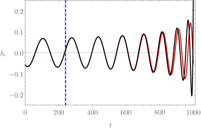
Figure 1: Gravitational waveforms for the spin-2 mode emitted by a BH binary inspiral. The $x$ axis gives the time $t$ (in arbitrary units); the $y$ axis measures the strain $h_{+}$ in units of $\mathcal{A}(r)\left(1+\cos^{2}\theta\right)/2$. The red curve corresponds to the prediction coming from GR. The black curve shows the spin-2 mode wave pattern for our higher-order gravity. The initial condition is such that the two strain curves coincide at $t=0$. The vertical dashed line marks the transition from the damping regime (on the left) to the oscillating regime, and the scalar mode is emitted from that point on. The transition depends on the factor $m_{-}c=3.43\times 10^{-2}$ corresponding to the time $t=240$. In our units, $\left(GM_{c}/c^{3}\right)=1$; for simplicity, we have set $\beta_{0}=0$.

The curve for the strain in our modified gravity model coincides with the curve for the strain from GR in the region to the left of the vertical dashed line of Fig. 1; in this region, the binary system does not emit the scalar-mode radiation. To the right of the vertical dashed line, the system gives off the extra scalar polarization; in this circumstance, the frequency of the strain in our modified gravity increases more rapidly than the frequency of the strain in GR. This increase is subtle, and it is noticeable only after a few oscillation periods (Fig. 1). The larger frequency increase leads to an earlier coalescence in our modified gravity.

We emphasize that the more the binary system approaches the merger, the weaker are the hypotheses used in our modelling, namely pointlike masses and nonrelativistic dynamics. In this sense, the region of the plot in Fig. 1 close to the merger should be taken as a qualitative description.

VII INSPIRAL PHASE OF BINARY PULSARS

The previous section dealt with black-hole binaries. The second possibility that we are going to contemplate here is a binary system composed of a pair of pulsars. Our focus is to constrain the coupling constants of our higher-order $R^{2}$ model utilizing observational data. In particular, we draw information from the observations of the Hulse-Taylor binary pulsar Hulse1975 ; Taylor1982 ; Weisberg2004 .

The motivation to treat binary pulsars in a separate section stems from the fact that their orbital dynamics is distinct from the one followed by binary black holes. In effect, the gravitational potential determining the orbits of the pair of neutron stars in the modified gravity context is not the Newtonian potential alone, as in Eq. (80), it but carries Yukawa-type terms, as we will see in Eq. (100) below.

We shall study two regimes: (i) the regime where the scalar mode propagates and the orbital dynamics modifications with respect to GR are maximum, and (ii) the regime where the scalar mode dies off and the spin-2 mode alone propagates; in this regime, we approach only small corrections to the ordinary gravitational potential. It is this second regime that allows us to observationally constrain the parameters in our modified gravity model.

VII.1 Gravitational potential and modified Kepler’s law

The complete relativistic solution in the context of modified gravity describing an extended static spherically symmetric mass has not been determined analytically yet. However, the gravitational potential for this type of source in the weak-field regime far from the source is already known: it bears corrections of the Yukawa type besides the conventional $\left(1/r\right)$ term. Accordingly, the modified potential of higher-order $R^{2}$ gravity in the nonrelativistic regime is Medeiros2020 :

$$V\left(r\right)=-\frac{Gm}{r}\left(1+a_{+}e^{-m_{-}r}+a_{-}e^{-m_{+}r}\right)\,,$$ (100)

where the parameters $m_{\pm}$ are given by Eq. (28) and

$$a_{\pm}=\pm\frac{1}{6}\left(\frac{1\pm\sqrt{1-\frac{4\beta_{0}}{3}}}{\sqrt{1-\frac{4\beta_{0}}{3}}}\right)\,.$$ (101)

In this paper, we will consider small corrections to the predictions by $R^{2}$ gravity coming from our higher-order $R^{2}$ gravity; this means that we will be taking $\beta_{0}\ll 1$ to achieve our main results. Within this condition, the masses $m_{\pm}$ are given by Eq. (30) and

$$a_{+}\simeq\frac{1}{3}\left(1+\frac{\beta_{0}}{3}\right)\qquad\text{and}\qquad a_{-}\simeq-\frac{\beta_{0}}{9}\qquad\left(\beta_{0}\ll 1\right)\,.$$ (102)

The potential (100) can be used to build the nonrelativistic equation of motion for the binary system. Assuming a circular orbit, where $r=R=\text{constant}$, this procedure leads to

$$\omega_{s}^{2}=\frac{Gm}{R^{3}}\left[1+a_{+}\left(1+m_{-}R\right)e^{-m_{-}R}+a_{-}\left(1+m_{+}R\right)e^{-m_{+}R}\right]\,,$$ (103)

which is an extended version of Kepler’s third law.

Equations (30) and (102) are then used in (103) to write down Kepler’s law in terms of the coupling constants $\kappa_{0}$ and $\beta_{0}$:

$$\omega_{s}^{2} \simeq\frac{Gm}{R^{3}}\left[1+\frac{1}{3}\left(1+\frac{\beta_{0}}{3}+\left(1+\frac{\beta_{0}}{2}\right)\Delta\right)\left(1-\frac{\beta_{0}}{6}\right)^{\Delta}e^{-\Delta}\right.$$

$$\left.-\frac{1}{3}\left(\frac{\beta_{0}}{3}+\sqrt{\frac{\beta_{0}}{3}}\left(1-\frac{\beta_{0}}{6}\right)\Delta\right)\left(1-\frac{\beta_{0}}{6}\right)^{-\sqrt{\frac{3}{\beta_{0}}}\Delta}e^{-\sqrt{\frac{3}{\beta_{0}}}\Delta}\right]\qquad\left(\beta_{0}\ll 1\right)\,,$$ (104)

where

$$\Delta\equiv\sqrt{\frac{\kappa_{0}}{3}}R\,.$$ (105)

The dimensionless quantity $\Delta$ is a measure of the importance of $R^{2}$ term relative to the Einstein-Hilbert term on an orbital scale. The greater (smaller) the $\Delta$, the smaller (greater) the influence of the modified gravity term at this scale.

Remark: The $R^{2}$-limit.— If $\beta_{0}\rightarrow 0$, Eq. (104) reads

$$\omega_{s}^{2}\simeq\frac{Gm}{R^{3}}\left[1+\frac{1}{3}\left(1+\Delta\right)e^{-\Delta}\right]\,.$$ (106)

This result is consistent with Eq. (40) in Ref. Naf2011 . $\blacksquare$

VII.1.1 The oscillatory limit

Let us study the limit of the generalized Kepler law [Eq. (104)] as $\Delta\ll 1$. This is interesting because we have seen in Sec. V.2 that the $\Phi_{-}$ solution displays two distinct regimes: the damped regime and the oscillatory regime. To select the oscillatory solution for $\Phi_{-}$ ultimately corresponds to taking $\Delta\ll 1$. In fact, the oscillatory regime occurs as

$$\frac{2\omega_{s}}{m_{-}c}>1\Rightarrow\frac{2\omega_{s}}{c}>\sqrt{\frac{\kappa_{0}}{3}}\left(1+\frac{\beta_{0}}{3}\right)^{1/2}\,,$$

where $2\omega_{s}$ is the frequency of the gravitational wave. For a binary system in a circular orbit, the tangential scalar velocity is $v=\omega_{s}R$. Then, the condition above is the same as

$$\frac{2}{R}\frac{v}{c}\gtrsim\sqrt{\frac{\kappa_{0}}{3}}\left(1+\frac{\beta_{0}}{6}\right)\overset{\frac{v}{c}\ll 1}{\Rightarrow}\Delta\left(1+\frac{\beta_{0}}{6}\right)\simeq\Delta\ll 1\,,$$ (107)

since $\beta_{0}\ll 1$.

In the case where $\Delta\ll 1$, we also have $e^{-\Delta}\simeq 1-\Delta\approx 1$, and terms scaling as $\beta_{0}\Delta$ may be neglected, since both $\beta_{0}$ and $\Delta$ are small. Hence, Eq. (104) reduces to

$$\omega_{s}^{2}\simeq\frac{Gm}{R^{3}}\left[\frac{4}{3}+\frac{\beta_{0}}{9}\epsilon\left(\Delta,\beta_{0}\right)\right]\,,$$

where

$$\epsilon\left(\Delta,\beta_{0}\right)\equiv\left[1-\left(1+\sqrt{\frac{3}{\beta_{0}}}\Delta\right)\left[\left(1-\frac{\beta_{0}}{6}\right)e\right]^{-\sqrt{\frac{3}{\beta_{0}}}\Delta}\right]\,.$$

A numerical analysis reveals that $0<\epsilon\left(\Delta,\beta_{0}\right)\leqslant 1$ by keeping in mind that $\beta_{0}\ll 1$. At most,

$$\omega_{s}^{2}\simeq\frac{Gm}{R^{3}}\left(\frac{4}{3}+\frac{\beta_{0}}{9}\right)\qquad\left(\Delta\ll 1\right)\,.$$ (108)

This expression is troublesome, since the factor $\left(4/3\right)$ enhances the orbital frequency in Kepler’s law in a way that should have been detected in orbital dynamics observations. This modification is significant enough to render our prediction incompatible with observations. This implies that our model in unphysical in the oscillatory regime for binary pulsars. The regime $\Delta\ll 1$ corresponds to the dominance of the $R^{2}$ term over the Einstein-Hilbert term in the action [Eq. (1)]. Reference Pechlaner1966 has shown a long time ago that this regime leads to the appearance of the factor 4/3 as a correction to the gravitational potential and Kepler’s third law. Moreover, the same reference proves that the weak-field regime of a theory built exclusively from the term $R^{2}$ is inconsistent. These arguments indicate that the physical regime is the one for $\Delta\gg 1$, which will be studied next.

VII.1.2 The damping limit

Now, the case $\Delta\gg 1$ will be considered. Because $\beta_{0}\ll 1$, we have $\Delta/\sqrt{\beta_{0}}\gg 1$, and Eq. (104) reduces to

$$\omega_{s}^{2}\simeq\frac{Gm}{R^{3}}\left[1+\frac{1}{3}\Delta e^{-\Delta}\left(1+\frac{\beta_{0}}{2}\right)\left(1-\frac{\beta_{0}}{6}\right)^{\Delta}\right]\qquad\left(\Delta\gg 1\right)\,,$$ (109)

which is very close to the Newtonian dynamics. This is the regime that will lead to constraints upon the additional coupling constants of our modified gravity model.

VII.2 The balance equation in the damping regime

We have already mentioned that the energy balance expression equates the power radiated to the time derivative of the orbital energy of the system. The power equation for a generic binary system in our modified gravity model was deduced in Sec. V.3. Here we begin by constructing the orbital energy $E_{\text{orbit}}=E_{\text{kin}}+\mu V\left(r\right)$ of the binary system in the context of our modified gravity. From Eqs. (100), (102), and (105),

$$E_{\text{orbit}} =\frac{1}{2}\mu\omega_{s}^{2}R^{2}$$

$$-\frac{Gm\mu}{R}\left\{1+\frac{1}{3}\left(1+\frac{\beta_{0}}{3}\right)\exp\left[-\left(1+\frac{\beta_{0}}{6}\right)\Delta\right]-\frac{\beta_{0}}{9}\exp\left[-\sqrt{\frac{3}{\beta_{0}}}\left(1-\frac{\beta_{0}}{6}\right)\Delta\right]\right\}\,.$$ (110)

Equation (110) assumes a circular orbit.

Using the modified Kepler law (104), the above equation turns to

$$E_{\text{orbit}} =-\frac{1}{2}\frac{Gm\mu}{R}\left\{1+\frac{1}{3}\left[\left(1+\frac{\beta_{0}}{3}\right)-\left(1+\frac{\beta_{0}}{2}\right)\Delta\right]e^{-\Delta\left(1+\frac{\beta_{0}}{6}\right)}\right.$$

$$\left.-\frac{\beta_{0}}{9}\left[1-\left(1-\frac{\beta_{0}}{6}\right)\sqrt{\frac{3}{\beta_{0}}}\Delta\right]e^{-\sqrt{\frac{3}{\beta_{0}}}\Delta\left(1-\frac{\beta_{0}}{6}\right)}\right\}\,,$$ (111)

where we have utilized the approximation

$$\left(1-\frac{\beta_{0}}{6}\right)^{\Delta}=e^{\Delta\ln\left(1-\frac{\beta_{0}}{6}\right)}\simeq e^{\Delta\left(-\frac{\beta_{0}}{6}\right)}\,.$$ (112)

We notice that $\dot{\Delta}=\Delta\left(\dot{R}/R\right)$ and obtain the time derivative of the orbital energy as

$$\frac{d}{dt}E_{\text{orbit}} =\frac{Gm\mu}{2R^{2}}\dot{R}\left\{1+\frac{1}{3}\left[\left(1+\frac{\beta_{0}}{3}\right)+\left(1+\frac{\beta_{0}}{2}\right)\Delta-\left(1+2\frac{\beta_{0}}{3}\right)\Delta^{2}\right]e^{-\Delta\left(1+\frac{\beta_{0}}{6}\right)}\right.$$

$$\left.-\frac{\beta_{0}}{9}\left[1+\left(1-\frac{\beta_{0}}{6}\right)\sqrt{\frac{3}{\beta_{0}}}\Delta-\left(1-\frac{\beta_{0}}{3}\right)\left(\sqrt{\frac{3}{\beta_{0}}}\Delta\right)^{2}\right]e^{-\sqrt{\frac{3}{\beta_{0}}}\Delta\left(1-\frac{\beta_{0}}{6}\right)}\right\}\,.$$ (113)

We equate Eq. (113) to Eq. (79), to get

$$\frac{64}{5}\frac{\mu}{m}\frac{\left(\omega_{s}R\right)^{6}}{c^{5}}\left\{1+\frac{\Theta\left(2\omega_{s}-m_{-}c\right)}{18}\sqrt{1-\left(\frac{m_{-}c}{2\omega_{s}}\right)^{2}}\left(1+\frac{\beta_{0}}{3}\right)\right\}=$$

$$=-\dot{R}\left\{1+\frac{1}{3}\left[\left(1+\frac{\beta_{0}}{3}\right)+\left(1+\frac{\beta_{0}}{2}\right)\Delta-\left(1+2\frac{\beta_{0}}{3}\right)\Delta^{2}\right]e^{-\Delta\left(1+\frac{\beta_{0}}{6}\right)}\right.$$

$$\left.-\frac{\beta_{0}}{9}\left[1+\left(1-\frac{\beta_{0}}{6}\right)\sqrt{\frac{3}{\beta_{0}}}\Delta-\left(1-\frac{\beta_{0}}{3}\right)\left(\sqrt{\frac{3}{\beta_{0}}}\Delta\right)^{2}\right]e^{-\sqrt{\frac{3}{\beta_{0}}}\Delta\left(1-\frac{\beta_{0}}{6}\right)}\right\}\,,$$ (114)

where $\omega_{s}=\omega_{s}\left(\Delta\right)$ is obtained via Eq. (104). Equation (114) expresses the energy balance in the regime of small higher-order corrections: $\beta_{0}\ll 1$. The left-hand side of this equation contains the spin-2 contribution (first term) and the contribution from the spin-0 mode (carrying the Heaviside function). The right-hand side of the equation accounts for the orbital energy loss, and the associated orbital radius decreasing, in the context of our higher-order $R^{2}$ model.

In principle, Eq. (114) could be explored in both the oscillatory regime and the damping regime. However, we have seen above that the oscillatory regime is unphysical for binary pulsars. Consequently, our focus will be on the damping regime for which $2\omega_{s}<m_{-}c\Rightarrow\Theta\left(2\omega_{s}-m_{-}c\right)=0$.

VII.2.1 Corrections to the time variation of the orbital period due to $R^{2}$ gravity

For the sake of simplicity, we shall consider the pure $R^{2}$-gravity case first. This is done by taking $\beta_{0}\rightarrow 0$ in Eqs. (114) and (104). Later on, we shall reintroduce the contribution of the higher-order terms through a small $\beta_{0}$. Accordingly, the energy balance equation reduces to

$$\frac{64}{5}\frac{\mu}{m}\frac{\left(R\omega_{s}\right)^{6}}{c^{5}}=-\dot{R}\left\{1+\frac{1}{3}\left[1+\Delta\left(1-\Delta\right)\right]e^{-\Delta}\right\}\,,$$ (115)

with

$$\omega_{s}^{2} \simeq\frac{Gm}{R^{3}}\left[1+\frac{1}{3}\left(1+\Delta\right)e^{-\Delta}\right]\,,$$ (116)

where the frequency $\omega_{s}$ can be expressed in terms of the orbital period $T$ as $\omega_{s}=2\pi/T$. By taking the time derivative of Eq. (116) and recalling Eq. (105), we get

$$\frac{2}{3}\frac{\dot{T}}{T}=\frac{\dot{R}}{R}\left\{1+\frac{1}{3}\frac{\Delta^{2}}{\left(1+\Delta\right)}\left[1-\left(\frac{T}{2\pi}\right)^{2}\frac{Gm}{R^{3}}\right]\right\}\,.$$ (117)

In GR, we miss the second term in the curly brackets. Our next step is to use Eq. (115) to replace $\dot{R}$ in Eq. (117); the result is

$$\dot{T}=-\frac{192\pi}{5}\left(\frac{GM_{c}}{c^{3}}\right)^{5/3}\left(\frac{T}{2\pi}\right)^{-5/3}g\left(\Delta\right)$$ (118)

where

$$g\left(\Delta\right)=\frac{\left\{1+\frac{1}{3}\left[1+\Delta+\frac{1}{3}\Delta^{2}\right]e^{-\Delta}\right\}}{\left\{1+\frac{1}{3}\left[1+\Delta-\Delta^{2}\right]e^{-\Delta}\right\}}\left[1+\frac{1}{3}\left(1+\Delta\right)e^{-\Delta}\right]^{2/3}\,.$$ (119)

Equation (119) is obtained after we make use of the modified Kepler’s law [Eq. (116)] multiple times. All changes to GR predictions due to our model are encapsulated in the function $g\left(\Delta\right)$. In fact, the $R^{2}$-gravity model tends to GR in the limit as $\kappa_{0}\rightarrow\infty$, thus $\Delta\rightarrow\infty$ and $\lim_{\Delta\rightarrow\infty}g\left(\Delta\right)=1$. Figure 2 shows the plot of $g=g\left(\Delta\right)$. The same figure displays the $g\left(\Delta\right)$ curve in the regime of large values of the argument, in which case Eq. (119) reduces to

$$g\left(\Delta\right)\approx 1+\frac{2}{9}\left(1+\Delta+2\Delta^{2}\right)e^{-\Delta}\,,\qquad\left(\Delta\gg 1\right)\,.$$ (120)

It is clear from Fig. 2 that the smaller the value of $\Delta$, the larger the differences with respect to GR. The parameter $\Delta$ can be estimated by using Eq. (118) and observational data. Our goal will be to determine the smallest value of $\Delta$ admissible by observations.

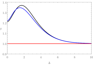
Figure 2: Plot of the function $g\left(\Delta\right)$ (black line) and its approximation for large values of $\Delta$ (blue line). The red line marks the result expected from GR: $g\left(\Delta\right)=1$.

In order to use Eq. (118) for comparison with observations, we need to account for the eccentricity of the binary system. For this reason, we will introduce (in a nonrigorous way) the eccentricity factor Weisberg2004 ; Maggiore2007 ; Peters1963

$$f\left(e\right)=\frac{1}{\left(1-e^{2}\right)^{7/2}}\left(1+\frac{73}{24}e^{2}+\frac{37}{96}e^{4}\right)$$ (121)

as a multiplicative term in the expression for the time variation of the orbital period [Eq. (118)]:

$$\dot{P}_{b,R^{2}\text{-gravity}}=\dot{T}\times f\left(e\right)\,.$$ (122)

Our idea is to constrain parameter $\Delta$ from the Hulse and Taylor binary pulsar PSR B1913+16 Hulse1975 ; Taylor1982 studied in detail in Ref. Weisberg2004 . The latter reference provides the parameter values in Table 1.

Parameter	Value
$e$	$0.6171338(4)$
$P_{b}\left(\text{days}\right)$	$0.322997448930(4)$
$m_{1}\left(M_{\astrosun}\right)$	$1.4414\pm 0.0002$
$m_{2}\left(M_{\astrosun}\right)$	$1.3867\pm 0.0002$
$\dot{P}_{b,\text{corrected}}\left(\text{s/s}\right)$	$-\left(2.4056\pm 0.0051\right)\times 10^{-12}$

Table 1: Parameters for the binary pulsar PSR B1913+16 as given by Weisberg2004 . The quantity $\dot{P}_{b,\text{corrected}}$ takes into account corrections to the observed period variation $\dot{P}_{b}$ due to the relative acceleration between the solar system and the binary pulsar.

There are four parameters in Table 1 affecting the evaluation of $\dot{P}_{b,R^{2}\text{-gravity}}$: namely, $e$, $P_{b}$, $m_{1}$, and $m_{2}$. When the uncertainties of these parameters are accounted for via error propagation, one concludes that the uncertainty in $\left(\dot{P}_{b,R^{2}\text{-gravity}}\times 10^{-12}\right)$ is of order $10^{-5}$. On the other hand, the uncertainty in $\left(\dot{P}_{b,\text{corrected}}\times 10^{-12}\right)$ is of order $10^{-3}$. Hence, we conclude that $\dot{P}_{b,\text{corrected}}$ dominates the uncertainties, the others being negligible by comparison. We will constrain the parameter $\Delta$ by considering that $\dot{P}_{b,R^{2}\text{-gravity}}$ should be within the interval

$$\dot{P}_{b,\text{min}}<\dot{P}_{b,R^{2}\text{-gravity}}<\dot{P}_{b,\text{max}}\,,$$

where

$$\dot{P}_{b,\text{min}}=\dot{P}_{b,\text{corrected}}-3\sigma=-2.42\times 10^{-12}\,\text{s/s}$$

and

$$\dot{P}_{b,\text{max}}=\dot{P}_{b,\text{corrected}}+3\sigma=-2.39\times 10^{-12}\,\text{s/s}\,.$$

The plot of $\dot{P}_{b,R^{2}\text{-gravity}}\left(\Delta\right)$ in Fig. 3 intercepts the horizontal line $\dot{P}_{b,\text{min}}$ at $\Delta_{\text{min}}=8.3$. The conclusion is that $\Delta$ should be greater than $8.3$ in order for $\dot{P}_{b,R^{2}\text{-gravity}}$ to be compatible with the observed time variation of the period within the $3\sigma$ uncertainty interval.

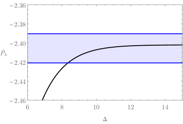
Figure 3: Plot of the predicted $\dot{P}_{b,R^{2}\text{-gravity}}$ as a function of $\Delta$. The lower (upper) straight line corresponds to $\dot{P}_{b,\text{min}}$ ($\dot{P}_{b,\text{max}}$). The region between the straight lines containing the curve $\dot{P}_{b,R^{2}\text{-gravity}}\left(\Delta\right)$ determines the domain of possible values for $\Delta$, the minimum of which corresponds to the intersection of the lower straight line with the curve $\dot{P}_{b,R^{2}\text{-gravity}}\left(\Delta\right)$ at $\Delta_{\text{min}}=8.3$.

In the following, we shall estimate the observational constraint upon $\kappa_{0}=3\left(\Delta/R\right)^{2}$ and check if the damping condition $2\omega_{s}<m_{-}c$ is satisfied. In order to do that, we have to estimate the orbital distance $R$. This value will lie in the interval set by the semimajor axis $a$ and the semiminor axis $b$ of the elliptical orbit of the Hulse-Taylor binary pulsar—see Ref. Taylor1982 . According to this reference, $R_{\text{max}}\equiv a=1.9490\times 10^{9}\,\text{m}$, and $R_{\text{min}}\equiv b=\sqrt{1-e^{2}}a=1.5336\times 10^{9}$, where we have used the eccentricity value in Table 1.

We know from Fig. 3 that $\Delta\geqslant 8.3$. Then, $\Delta_{\text{min}}=8.3$, and the more restrictive estimate upon $R^{2}$-term coupling is achieved by taking $R=R_{\text{min}}$:

$$\kappa_{0}>3\left(\frac{\Delta_{\text{min}}}{R_{\text{min}}}\right)^{2}\simeq 8.8\times 10^{-17}\,\text{m}^{-2}\qquad\text{or}\qquad\frac{1}{\kappa_{0}}\lesssim 1.1\times 10^{16}\,\text{m}^{2}\,.$$ (123)

It is interesting to compare this constraint to other results available in the literature. The estimates related to GW are $a_{2}<1.2\times 10^{18}\,\text{m}^{2}$ in Ref. Berry2011 and $a<1.7\times 10^{17}\,\text{m}^{2}$ in Ref. Naf2011 , with the notational correspondences $\left(1/\kappa_{0}\right)\leftrightarrow a_{2}\leftrightarrow a$, respectively. Notice that we obtain an order-of-magnitude improvement in the constraint of $\left(1/\kappa_{0}\right)$; however, this should be taken with a grain of salt, since we have introduced the eccentricity factor in an ad hoc fashion. In a future work, we intend to refine this estimate by computing the effect of eccentricity in a deductive, rigorous way in our analysis.

Now, we will check if the damping constraint ($2\omega_{s}<m_{-}c$) is satisfied by our estimate of $\kappa_{0}$. First, we use the lowest value of $\kappa_{0}$ in Eq. (123) to obtain

$$m_{-}=\sqrt{\frac{\kappa_{0}}{3}}\Rightarrow m_{-}c>1.6\,\text{s}^{-1}\,.$$ (124)

On the other hand, utilizing the observed period in Table 1,

$$\omega_{s}=\frac{2\pi}{T}\Rightarrow 2\omega_{s}=\frac{4\pi}{P_{b}\left(\text{s}\right)}=4.5\times 10^{-4}\,\text{s}^{-1}\,.$$ (125)

By comparing Eqs. (124) and (125), we conclude that $2\omega_{s}<m_{-}c$, consequently checking the validity of our analysis.

VII.2.2 Corrections to the time variation of the orbital period due to higher-order $R^{2}$ gravity

The development above on the pure quadratic-curvature scalar case shows that $\Delta\gtrsim 8$. This will also be true when one adds to the $R^{2}$-gravity model the higher-order contributions carrying the coupling constant $\beta_{0}$. In fact, the terms scaling with $\beta_{0}$ in the action of our higher-order quadratic-curvature scalar model are considered as a small correction to those accompanied by $R^{2}$-gravity coupling $\kappa_{0}$. Accordingly, by considering $\beta_{0}\ll 1$ and $\Delta\gtrsim 8$ in Eqs. (114) and (104), and following a procedure similar to the one in the previous subsection, we get

$$\dot{T}\simeq -\frac{192\pi}{5}\left(\frac{GM_{c}}{c^{3}}\right)^{5/3}\left(\frac{T}{2\pi}\right)^{-5/3}$$

$$\times\left\{1+\frac{2}{9}\left[\left(1+\frac{\beta_{0}}{3}\right)+\left(1+\frac{\beta_{0}}{2}\right)\Delta+2\left(1+2\frac{\beta_{0}}{3}\right)\Delta^{2}\right]e^{-\Delta\left(1+\frac{\beta_{0}}{6}\right)}\right\}\,.$$ (126)

Note that Eq. (126) obediently reduces to Eq. (118), with $g\left(\Delta\right)$ given by Eq. (120) in the limit as $\beta_{0}\rightarrow 0$.

The interval of values assumed by the pair $\left(\beta_{0},\Delta\right)$ can be estimated by using Eq. (126) and observational data in much the same way as is done in the case of pure $R^{2}$-type corrections to GR (Sec. VII.2.1). We allow $\beta_{0}$ to vary in the interval $\left[0,3/4\right]$ and estimate the values admitted by $\Delta$ that satisfy $\dot{P}_{b,\text{min}}<\dot{P}_{b,\text{higher-order}}<\dot{P}_{b,\text{max}}$, where $\dot{P}_{b,\text{higher-order}}=\dot{T}\times f\left(e\right)$. Thereafter, we can transfer the constraint upon $\Delta$ onto the coupling $\kappa_{0}$. This is done by estimating $R=R_{\text{min}}$ and using $\kappa_{0}=3\left(\Delta_{\text{min}}/R_{\text{min}}\right)^{2}$, with the understanding that now $\Delta_{\text{min}}=\Delta_{\text{min}}\left(\beta_{0}\right)$. The plot of $\left(1/\kappa_{0}\right)$ as a function of $\beta_{0}$ is shown in Fig. 4.

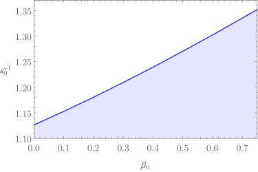
Figure 4: Plot of $\beta_{0}\times\kappa_{0}^{-1}$. The $y$ axis contains the values of $\kappa_{0}^{-1}$ in units of $\left(10^{16}\,\text{m}^{2}\right)$. The allowed region for the parameter space is the shadowed region below the curve.

Even though $\beta_{0}$ can take values in the interval $\left[0,3/4\right]$, we have assumed a small $\beta_{0}$ in our approximations along the computations. For this reason, the most reliable region of the parameter space in Fig. 4 is close to the origin.

VIII FINAL COMMENTS

In this paper, we have studied the gravitational waves emitted by binary systems in the context of the higher-order quadratic-curvature scalar model built from an action integral involving the Einstein-Hilbert term plus $R^{2}$ and $R\square R$ contributions. We have assumed nonrelativistic motion of the pair of point particles in the binary system and a circular orbit.

The gravitational wave solution was computed by considering the dominant terms in the multipole expansion. It exhibits two modes, $\Phi_{-}$ and $\Phi_{+}$, for the decomposed massive scalar field $\Phi$ in addition to the expected spin-2 mode $\tilde{h}_{\mu\nu}$. The spin-0 modes feature two different behaviors: the oscillatory regime, which plays the actual GW part, and the damped regime, which is exponentially suppressed.

In order to study the power radiated in the form of gravitational waves, it was necessary to build the higher-order energy-momentum pseudotensor, after which we established the balance equation.

We have determined the wave pattern given off by black-hole binaries during the inspiral phase. The strain displays an increase in amplitude and frequency that is a bit more pronounced than in the relativistic case; the chirp occurs before the ordinary GR prediction. This effect is a result of the extra channeling through the scalar mode: besides the power radiated by $\tilde{h}_{\mu\nu}$-type emission, there is the energy loss via the radiation of the spin-0 field $\Phi$.

Our modification in the description of gravity also affects the orbital dynamics of a binary pulsar system. The change in the orbital dynamics alters the balance equation and, as a consequence, the differential equation of the orbital period. The time variation in the orbital period of the Hulse-Taylor binary pulsar was used to constrain the coupling constants $\kappa_{0}$ and $\beta_{0}$ related to the $R^{2}$ and $R\square R$ terms.

In fact, the coupling constant $\left(1/\kappa_{0}\right)$ of the $R^{2}$ term was restricted to $\kappa_{0}^{-1}\lesssim 1.1\times 10^{16}\,\text{m}^{2}$. This constraint is several orders of magnitude less restrictive than the one offered by the Eöt-Wash torsion balance experiment Kapner2007 , namely $a\lesssim{10}^{-9}\,\text{m}^{2}$. This estimation is based on the result $\sqrt{3a}=\lambda\gtrsim 56\,\mu\text{m}$ is excluded within 95 % confidence level according to Ref. Kapner2007 . The difference is rooted in the fact that the data related to GW are astrophysical in nature, while torsion balance experiments probe earthly gravity effects. Even though our constraint is much less restrictive, it is of fundamental importance to test alternative models of gravity in as many different scales as possible. This is a sensitive aspect indeed, given that our model (or extensions of it) might feature a screening mechanism Jana2019 ; Khoury2004 ; this possibility remains to be checked and explored in a future work. In any case, our constraint on $\kappa_{0}^{-1}$ is about 1 order of magnitude better than the ones given in Refs. Berry2011 ; Naf2011 , which use similar approaches to ours.

In this work, we assume that the contribution of the term $R\square R$ to the modified gravity model is incremental. Accordingly, the associated coupling constant $\beta_{0}$ should be small. We have shown that the small-valued $\beta_{0}$ modifies very little the results obtained in the analysis of the gravitational waves in the pure $\left(R+R^{2}\right)$ case.

It should be mentioned that the constraint over $\kappa_{0}$ lacks rigor, given the fact that we have introduced the eccentricity function $f\left(e\right)$ in an ad hoc fashion. This weak point in our treatment automatically motivates a future work in which the noncircular orbits of the pair of astrophysical bodies in the binary system are considered from the start. It is well known from the standard GR treatment that taking into account elliptical orbits leads to the emission of GW with a multitude of frequencies. As a result of considering eccentric orbits in our modified gravity model, we might conclude that the gravitational waves present a spin-0 oscillatory mode with frequencies high enough to meaningfully contribute to the power radiated within the observational bounds. This remains to be checked.

Appendix A RESOLVING $\Phi_{-}$ FIELD EQUATION

Let us consider the scalar equation for $\Phi_{-}$, Eq. (27) from Sec. III:

$$\left(\square-m_{-}^{2}\right)\Phi_{-}=Q\,,$$ (127)

where $Q\equiv-\frac{\chi}{3}T$. The solution is of the form

$$\Phi_{-}\left(x^{\mu}\right)=\int G_{\Phi}\left(x^{\mu};x^{\prime\mu}\right)Q\left(x^{\prime\mu}\right)d^{4}x^{\prime}\,,$$ (128)

where the differential equation for the Green’s function $G_{\Phi}\left(x^{\mu};x^{\prime\mu}\right)$,

$$\left(\square-m_{-}^{2}\right)G_{\Phi}\left(x^{\nu};x^{\prime\nu}\right)=\delta^{4}\left(x^{\nu}-x^{\prime\nu}\right)\,,$$ (129)

is solved via the Fourier transform

$$G_{\Phi}\left(x^{\nu};x^{\prime\nu}\right)=\frac{1}{\left(2\pi\right)^{2}}\int e^{iq_{\mu}\left(x^{\mu}-x^{\prime\mu}\right)}g_{\Phi}\left(q_{\nu}\right)d^{4}q\,.$$ (130)

Plugging Eq. (130) into Eq. (129) and utilizing the integral form of the delta function, we obtain

$$g_{\Phi}\left(q_{\nu}\right)=\frac{1}{\left(2\pi\right)^{2}\left[-q_{\mu}q^{\mu}-m_{-}^{2}\right]}\,.$$ (131)

Substituting Eq. (131) into Eq. (130), we find

$$G_{\Phi}\left(x^{\nu};x^{\prime\nu}\right)=\frac{1}{\left(2\pi\right)^{4}}\int d^{3}\mathbf{q}e^{i\mathbf{q}.\left(\mathbf{x}-\mathbf{x}^{\prime}\right)}\left\{\int dq_{0}e^{iq_{0}\left(x^{0}-x^{\prime 0}\right)}\frac{1}{\left[\left(q_{0}\right)^{2}-\mathbf{q}^{2}-m_{-}^{2}\right]}\right\}\,,$$ (132)

which depends on the integral

$$I_{0}=\int_{-\infty}^{+\infty}dq_{0}e^{iq_{0}\left(x^{0}-x^{\prime 0}\right)}\frac{1}{\left[\left(q_{0}\right)^{2}-p^{2}\right]}\,,$$ (133)

where

$$p^{2}\equiv\mathbf{q}^{2}+m_{-}^{2}\,.$$ (134)

The integral $I_{0}$ is solved by analytical extension and the use of the Cauchy integral formula—see Ref. Jackson1999 . Physical arguments lead us to choose the retarded Green’s function, and to the result

$$I_{0}=\begin{cases}0\,,&x^{0}<x^{\prime 0}\\ -\frac{2\pi}{p}\sin\left[p\left(x^{0}-x^{\prime 0}\right)\right]\,,&x^{0}>x^{\prime 0}\end{cases}\,.$$ (135)

Inserting Eq. (135) into the expression (132) for $G_{\Phi}\left(x^{\nu};x^{\prime\nu}\right)$ gives

$$G_{\Phi}\left(x^{\nu};x^{\prime\nu}\right)=-\frac{1}{\left(2\pi\right)^{3}}\int q^{2}\sin\theta dqd\theta d\phi\frac{e^{iqs\cos\theta}}{\sqrt{\mathbf{q}^{2}+m_{-}^{2}}}\sin\left[\sqrt{\mathbf{q}^{2}+m_{-}^{2}}c\tau\right]\,,$$ (136)

where

$$c\tau\equiv\left(x^{0}-x^{\prime 0}\right)=\left(ct-ct^{\prime}\right)\,,$$ (137)

$$s=\left|\mathbf{s}\right|=\left|\mathbf{x}-\mathbf{x}^{\prime}\right|\,,$$ (138)

and we take $\mathbf{q}$ in spherical coordinates. Moreover, we have set the $z$ axis in the direction of vector $\mathbf{s}$, such that $\mathbf{q}\cdot\left(\mathbf{x}-\mathbf{x}^{\prime}\right)\equiv\mathbf{q}\cdot\mathbf{s}=qs\cos\theta$.

By integrating over the angular coordinates, Eq. (136) takes on the form

$$G_{\Phi}\left(x^{\nu};x^{\prime\nu}\right)=-\frac{2}{\left(2\pi\right)^{2}}\frac{1}{s}\int_{0}^{\infty}qdq\sin\left(qs\right)\frac{\sin\left(E_{q}c\tau\right)}{E_{q}}\,,$$ (139)

where

$$E_{q}\equiv\sqrt{q^{2}+m_{-}^{2}}\,.$$ (140)

The massless case, $m_{-}=0$, is well known from the literature. The result consistent with $x^{0}>x^{\prime 0}$ is

$$G_{\Phi}\left(x^{\nu};x^{\prime\nu}\right)=-\frac{1}{4\pi}\frac{1}{s}\delta\left(s-c\tau\right)\,,\qquad\left(m_{-}=0\right)\,.$$ (141)

For the complete massive case, it is useful to write the sines in Eq. (139) in terms of exponentials and use the identity

$$\int_{-\infty}^{\infty}\frac{q}{E_{q}}dq\exp\left[-i\left(E_{q}c\tau-qs\right)\right]=-i\frac{\partial}{\partial s}\int_{-\infty}^{\infty}dq\frac{\exp\left[-i\left(E_{q}c\tau-qs\right)\right]}{E_{q}}$$

to write

$$G_{\Phi}\left(x^{\nu};x^{\prime\nu}\right)=\frac{i}{8\pi^{2}}\frac{1}{s}\frac{\partial}{\partial s}\left[\int_{-\infty}^{\infty}dq\frac{\exp\left[-i\left(E_{q}c\tau-qs\right)\right]}{E_{q}}-\int_{-\infty}^{\infty}dq\frac{\exp\left[i\left(E_{q}c\tau-qs\right)\right]}{E_{q}}\right]\,.$$ (142)

The change of variables Greiner2009

$$E_{q}=m_{-}\cosh\eta\,,\qquad\text{and}\qquad q=m_{-}\sinh\eta$$ (143)

is suggestive, once it respects $E_{q}^{2}-q^{2}=m_{-}^{2}$ , cf. Eq. (140). Then,

$$G_{\Phi}\left(x^{\nu};x^{\prime\nu}\right) =\frac{i}{8\pi^{2}}\frac{1}{s}\frac{\partial}{\partial s}\left[\int_{-\infty}^{\infty}d\eta\exp\left[-im_{-}\left(c\tau\cosh\eta-s\sinh\eta\right)\right]\right.$$

$$\left.-\int_{-\infty}^{\infty}d\eta\exp\left[im_{-}\left(c\tau\cosh\eta-s\sinh\eta\right)\right]\right]\,.$$ (144)

We should have $\tau>0$; otherwise, the Green’s function is null.

There are three possible cases:

1. Timelike separation: $c\tau>s$. In this case, it is always true that $\tau>0$, because $s=\left|\mathbf{x}-\mathbf{x}^{\prime}\right|>0$. It is convenient to define the variable $\theta$ such that

   $$c\tau=\sqrt{\left(c\tau\right)^{2}-s^{2}}\cosh\theta\,,\qquad\text{and}\qquad s=\sqrt{\left(c\tau\right)^{2}-s^{2}}\sinh\theta\,.$$ (145)

   Hence, $\left(c\tau\cosh\eta-s\sinh\eta\right)=\sqrt{\left(c\tau\right)^{2}-s^{2}}\cosh\left(\eta-\theta\right)$. Furthermore, by defining

   $$u=\left(\eta-\theta\right)\,,$$ (146)

   we cast Eq. (144) into the form

   $$G_{\Phi}\left(x^{\nu};x^{\prime\nu}\right)=\frac{1}{4\pi^{2}}\frac{1}{s}\frac{\partial}{\partial s}\int_{-\infty}^{\infty}du\sin\left[m_{-}\sqrt{\left(c\tau\right)^{2}-s^{2}}\cosh u\right]\,.$$ (147)

   Using the integral representation of the Bessel function Gradshteyn2007 ,

   $$J_{0}\left(z\right)=\frac{1}{\pi}\int_{-\infty}^{\infty}\sin\left(z\cosh u\right)du\qquad\left(\text{Re}[z]>0\right)\,,$$

   and the recurrency relation,

   $$\frac{dJ_{0}\left(z\right)}{dz}=-J_{1}\left(z\right)\,,$$

   in Eq. (147), we finally obtain

   $$G_{\Phi}\left(x^{\nu};x^{\prime\nu}\right)=\frac{1}{4\pi}\frac{m_{-}}{\sqrt{\left(c\tau\right)^{2}-s^{2}}}J_{1}\left(m_{-}\sqrt{\left(c\tau\right)^{2}-s^{2}}\right)\qquad\left(c\tau>s\right)\,.$$ (148)

2. Spacelike separation: $c\tau<s$. In this case, the convenient change of variables is

   $$c\tau=\sqrt{s^{2}-\left(c\tau\right)^{2}}\sinh\theta\,\qquad\text{and}\qquad s=\sqrt{s^{2}-\left(c\tau\right)^{2}}\cosh\theta\,.$$ (149)

   Following an analogous reasoning to the previous case, we have

   $$G_{\Phi}\left(x^{\nu};x^{\prime\nu}\right)=-\frac{1}{4\pi^{2}}\frac{1}{s}\frac{\partial}{\partial s}\left\{\int_{-\infty}^{\infty}du\sin\left[m_{-}\sqrt{s^{2}-\left(c\tau\right)^{2}}\sinh u\right]\right\}=0\qquad\left(0<c\tau<s\right)\,,$$ (150)

   where $u$ is defined in Eq. (146).

3. Lightlike case: $c\tau=s$. The lightlike case corresponds to a massless particle moving on the light cone. This case was previously treated; the corresponding Green’s function is Eq. (141).

All the possibilities can be unified by utilizing the Heaviside step function

$$\Theta\left(\xi\right)=\begin{cases}0,&\xi<0\\ 1,&\xi>0\end{cases}\,.$$ (151)

Therefore,

$$G_{\Phi}\left(x^{\nu};x^{\prime\nu}\right)=-\frac{1}{4\pi}\frac{1}{c}\frac{1}{s}\delta\left(\tau-\frac{s}{c}\right)+\frac{1}{4\pi}\Theta\left(\tau-\frac{s}{c}\right)\frac{1}{c}\frac{m_{-}}{\sqrt{\tau^{2}-\left(\frac{s}{c}\right)^{2}}}J_{1}\left(m_{-}c\sqrt{\tau^{2}-\left(\frac{s}{c}\right)^{2}}\right)\,.$$ (152)

This is the complete Green’s function that solves Eqs. (127) through (128).

Appendix B THE SPIN-0 FIELD $\Phi_{-}$

In Eq. (49) of Sec. IV.3, we have written $\Phi_{-}$ as a multipole decomposition $\Phi_{-}=\Phi_{-}^{M}+\Phi_{-}^{D}+\Phi_{-}^{Q}+\cdots$. It can be concluded from Eqs. (50), (51), and (59) that the monopole term $\Phi_{-}^{M}$ and dipole mode $\Phi_{-}^{D}$ do not contribute to the gravitational wave emitted by a binary system in the center-of-mass reference frame: $\Phi_{-}^{M}$ does not radiate, and $\Phi_{-}^{D}$ is zero.

The quadrupole mode will be the dominant contribution for the scalar mode of the gravitational radiation,

$$\Phi_{-}\left(\mathbf{x},t\right)=\Phi_{-}^{Q}\left(\mathbf{x},t\right)\equiv\Phi_{-}^{Q_{1}}\left(\mathbf{x},t\right)+\Phi_{-}^{Q_{2}}\left(\mathbf{x},t\right),$$ (153)

where

$$\Phi_{-}^{Q_{1}}\left(\mathbf{x},t\right)=\frac{2}{3}\frac{G}{c^{4}}\frac{1}{r}\left[\frac{1}{2}n^{i}n^{j}\left.\frac{\partial^{2}\mathcal{M}^{ij}}{\partial t^{2}}\right|_{t_{r}}\right]$$ (154)

and

$$\Phi_{-}^{Q_{2}}\left(\mathbf{x},t\right)=-m_{-}\frac{2}{3}\frac{G}{c^{4}}\int_{0}^{\infty}d\tau_{r}F\left(\tau_{r}\right)\left[\frac{1}{2}n^{i}n^{j}\left.\frac{\partial^{2}\mathcal{M}^{ij}}{\partial t^{2}}\right|_{\zeta}\right]\,,$$ (155)

as per Eqs. (45) and (52). We recall that $\zeta=\left(t-\frac{r}{c}\right)-\tau_{r}$. The unit vector $n_{i}$ points out orthogonally from the plane of the orbit, forming an angle $\theta$ with the line of sight, cf. Eq. (61). From Eqs. (60) and (59), we calculate the time derivatives of $\mathcal{M}^{ij}$:

$$\ddot{\mathcal{M}}^{11}\left(t\right)=-2\mu R^{2}\omega_{s}^{2}\cos\left(2\omega_{s}t\right)=-\ddot{\mathcal{M}}^{22}\,,\qquad\ddot{\mathcal{M}}^{12}\left(t\right)=-2\mu R^{2}\omega_{s}^{2}\sin\left(2\omega_{s}t\right)\,.$$ (156)

Therefore,

$$\left[\frac{1}{2}n^{i}n^{j}\left.\frac{\partial^{2}\mathcal{M}^{ij}}{\partial t^{2}}\right|_{\xi}\right]=\left[\mu R^{2}\omega_{s}^{2}\sin^{2}\theta\cos\left(2\omega_{s}\xi+2\phi\right)\right]\,.$$ (157)

From Eq. (157), we immediately obtain

$$\Phi_{-}^{Q_{1}}\left(\mathbf{x},t\right)=\frac{2\mu R^{2}\omega_{s}^{2}}{3}\frac{G}{c^{4}}\frac{1}{r}\sin^{2}\theta\cos\left(2\omega_{s}t_{r}+2\phi\right)$$ (158)

and

$$\Phi_{-}^{Q_{2}}\left(\mathbf{x},t\right) =-m_{-}\frac{2}{3}\frac{G}{c^{4}}\mu R^{2}\omega_{s}^{2}\sin^{2}\theta$$

$$\times\int_{0}^{\infty}d\tau_{r}\frac{J_{1}\left(m_{-}c\sqrt{2\tau_{r}}\sqrt{\frac{\tau_{r}}{2}+\frac{r}{c}}\right)}{\sqrt{2\tau_{r}}\sqrt{\frac{\tau_{r}}{2}+\frac{r}{c}}}\cos\left(-2\omega_{s}\left[\tau_{r}-\left(t-\frac{r}{c}\right)\right]+2\phi\right)\,.$$ (159)

Hereafter, we will deal with Eq. (159). The integration variable can be changed to

$$\tau_{r}=\frac{x}{m_{-}c}-\frac{r}{c}\,,$$ (160)

so that

$$\Phi_{-}^{Q_{2}}\left(\mathbf{x},t\right)=-m_{-}\frac{2}{3}\frac{G}{c^{4}}\mu R^{2}\omega_{s}^{2}\sin^{2}\theta\left\{\cos\left[2\omega_{s}t+2\phi\right]I_{1}\left(r\right)+\sin\left[2\omega_{s}t+2\phi\right]I_{2}\left(r\right)\right\}\,,$$ (161)

where we denote

$$I_{1}\left(r\right)=I_{1}\left(a,b\right)\equiv\int_{a}^{\infty}dx\frac{J_{1}\left(\sqrt{x^{2}-a^{2}}\right)}{\sqrt{x^{2}-a^{2}}}\cos\left(bx\right)$$ (162)

and

$$I_{2}\left(r\right)=I_{2}\left(a,b\right)\equiv\int_{a}^{\infty}dx\frac{J_{1}\left(\sqrt{x^{2}-a^{2}}\right)}{\sqrt{x^{2}-a^{2}}}\sin\left(bx\right)\,,$$ (163)

with the definitions

$$a\equiv m_{-}r\,,\quad\text{and}\quad b\equiv\frac{2\omega_{s}}{m_{-}c}\,.$$ (164)

In order to solve $I_{1}\left(a,b\right)$ and $I_{2}\left(a,b\right)$, consider the following integrals in Ref. Gradshteyn2007 :

$$H_{1}\left(a,b\right)=b\int_{a}^{\infty}dxJ_{0}\left(\sqrt{x^{2}-a^{2}}\right)\cos\left(bx\right)=\begin{cases}\frac{b}{\sqrt{1-b^{2}}}\exp\left[-a\sqrt{1-b^{2}}\right]\,,&0<b<1\\ -b\frac{\sin\left(a\sqrt{b^{2}-1}\right)}{\sqrt{b^{2}-1}}\,,&b>1\end{cases}$$ (165)

and

$$H_{2}\left(a,b\right)=b\int_{a}^{\infty}dxJ_{0}\left(\sqrt{x^{2}-a^{2}}\right)\sin\left(bx\right)=\begin{cases}0\,,&0<b<1\\ b\frac{\cos\left(a\sqrt{b^{2}-1}\right)}{\sqrt{b^{2}-1}}\,,&b>1\end{cases}\,.$$ (166)

Our strategy will be to solve $I_{1}\left(a,b\right)$ first by utilizing Eq. (165). Accordingly, let us work out the integral in

$$H_{1}\left(a,b\right)=b\int_{a}^{\infty}J_{0}\left(\sqrt{x^{2}-a^{2}}\right)\cos\left(bx\right)dx\,.$$

We perform an integration by parts, recalling the following properties of the Bessel function:

$$\frac{d}{dz}J_{0}\left(z\right)=-J_{1}\left(z\right)\,,\quad J_{0}\left(0\right)=1\quad\text{and}\quad\lim_{x\rightarrow\infty}J_{0}\left(x\right)=0\,.$$

The result is

$$H_{1}\left(a,b\right)=-\sin\left(ab\right)+\int_{a}^{\infty}\frac{x}{\sqrt{x^{2}-a^{2}}}J_{1}\left(\sqrt{x^{2}-a^{2}}\right)\sin\left(bx\right)dx\,.$$

We will recognize $I_{1}\left(a,b\right)$ in the expression above after we integrate it with respect to $b$:

$$\int H_{1}db=\frac{1}{a}\cos\left(ab\right)-\int_{a}^{\infty}\frac{J_{1}\left(\sqrt{x^{2}-a^{2}}\right)}{\sqrt{x^{2}-a^{2}}}\cos\left(bx\right)dx\,,$$

or, due to Eq. (162),

$$I_{1}\left(a,b\right)=-\int H_{1}db+\frac{1}{a}\cos\left(ab\right)\,.$$ (167)

The integral $\int H_{1}db$ appearing in Eq. (167) is evaluated with the help of the results on the right-hand side of Eq. (165):

$$\int H_{1}db=\begin{cases}\frac{1}{a}\exp\left[-a\sqrt{1-b^{2}}\right]+K_{1}\,,&0<b<1\\ \frac{1}{a}\cos\left[a\sqrt{b^{2}-1}\right]+C_{1}\,,&b>1\end{cases}\,,$$

where $K_{1}$ and $C_{1}$ are integration constants. Plugging back in the definitions of $a$ and $b$ in terms of parameters of our model—Eq. (164)—leads to

$$I_{1}\left(r\right)=\begin{cases}-\frac{1}{m_{-}r}\left[\exp\left(-m_{-}r\sqrt{1-\left(\frac{2\omega_{s}}{m_{-}c}\right)^{2}}\right)-\cos\left(\frac{2\omega_{s}r}{c}\right)\right]-K_{1}\,,&2\omega_{s}<m_{-}c\\ -\frac{1}{m_{-}r}\left[\cos\left(m_{-}r\sqrt{\left(\frac{2\omega_{s}}{m_{-}c}\right)^{2}-1}\right)-\cos\left(\frac{2\omega_{s}r}{c}\right)\right]-C_{1}\,,&2\omega_{s}>m_{-}c\end{cases}\,.$$ (168)

The integral $I_{2}\left(r\right)$ in Eq. (163) is solved by using Eq. (166) for $H_{2}\left(a,b\right)$. In a procedure completely analogous to what we have done above for $I_{1}\left(r\right)$, we compute

$$I_{2}\left(r\right)\begin{cases}\frac{1}{m_{-}r}\sin\left(\frac{2\omega_{s}r}{c}\right)-K_{2}\,,&2\omega_{s}<m_{-}c\\ -\frac{1}{m_{-}r}\left[\sin\left(m_{-}r\sqrt{\left(\frac{2\omega_{s}}{m_{-}c}\right)^{2}-1}\right)-\sin\left(\frac{2\omega_{s}r}{c}\right)\right]-C_{2}\,,&2\omega_{s}>m_{-}c\end{cases}\,,$$ (169)

with $K_{2}$ and $C_{2}$ being integration constants.

Now, we plug Eqs. (168) and (169) into Eq. (161) for $\Phi_{-}^{Q_{2}}$ and separate the result into two regimes:

• For $m_{-}c>2\omega_{s}$,

  $$\Phi_{-}^{Q_{2}}\left(\mathbf{x},t\right) =m_{-}\frac{2}{3}\frac{G}{c^{4}}\mu R^{2}\omega_{s}^{2}\sin^{2}\theta\cos\left[2\omega_{s}t+2\phi\right]$$

  $$\times\left\{\frac{1}{m_{-}r}\left[\exp\left(-m_{-}r\sqrt{1-\left(\frac{2\omega_{s}}{m_{-}c}\right)^{2}}\right)-\cos\left(\frac{2\omega_{s}r}{c}\right)\right]+K_{1}\right\}$$

  $$+m_{-}\frac{2}{3}\frac{G}{c^{4}}\mu R^{2}\omega_{s}^{2}\sin^{2}\theta\sin\left[2\omega_{s}t+2\phi\right]\left\{-\frac{1}{m_{-}r}\sin\left(\frac{2\omega_{s}r}{c}\right)+K_{2}\right\}\,.$$ (170)

• For $m_{-}c<$ $2\omega_{s}$,

  $$\Phi_{-}^{Q_{2}}\left(\mathbf{x},t\right) =m_{-}\frac{2}{3}\frac{G}{c^{4}}\mu R^{2}\omega_{s}^{2}\sin^{2}\theta\cos\left[2\omega_{s}t+2\phi\right]$$

  $$\times\left\{\frac{1}{m_{-}r}\left[\cos\left(m_{-}r\sqrt{\left(\frac{2\omega_{s}}{m_{-}c}\right)^{2}-1}\right)-\cos\left(\frac{2\omega_{s}r}{c}\right)\right]+C_{1}\right\}$$

  $$+m_{-}\frac{2}{3}\frac{G}{c^{4}}\mu R^{2}\omega_{s}^{2}\sin^{2}\theta\sin\left[2\omega_{s}t+2\phi\right]$$

  $$\times\left\{\frac{1}{m_{-}r}\left[\sin\left(m_{-}r\sqrt{\left(\frac{2\omega_{s}}{m_{-}c}\right)^{2}-1}\right)-\sin\left(\frac{2\omega_{s}r}{c}\right)\right]+C_{2}\right\}\,.$$ (171)

At this point, it is necessary to set the constants $K_{1,2}$ to recover the suitable limits. As $m_{-}\rightarrow\infty\Rightarrow\kappa_{0}\rightarrow\infty$, we must recover the GR results, which means that

$$\lim_{m_{-}\rightarrow\infty}\left(\Phi_{-}^{Q_{1}}+\Phi_{-}^{Q_{2}}\right)=0\Rightarrow\lim_{m_{-}\rightarrow\infty}\Phi_{-}^{Q_{2}}=-\lim_{m_{-}\rightarrow\infty}\Phi_{-}^{Q_{1}}$$

This can be achieved if $K_{1}=K_{2}=0$. Moreover, by imposing continuity of Eqs. (171) and (170) at $m_{-}c=2\omega_{s}$, we conclude that $C_{1}=C_{2}=0$. Under these choices, and substituting Eqs. (158), (171), and (170) into Eq. (153), it follows that

$$\Phi_{-}\left(\mathbf{x},t\right)=\begin{cases}\frac{1}{6}\frac{1}{r}\frac{4G}{c^{4}}\mu\omega_{s}^{2}R^{2}\sin^{2}\theta\cos\left(2\omega_{s}t+2\phi\right)\left[\exp\left(-m_{-}r\sqrt{1-\left(\frac{2\omega_{s}}{m_{-}c}\right)^{2}}\right)\right]\,,&\left(2\omega_{s}<m_{-}c\right)\\ \frac{1}{6}\frac{1}{r}\frac{4G}{c^{4}}\mu\omega_{s}^{2}R^{2}\sin^{2}\theta\cos\left[2\omega_{s}\left(t-\frac{r}{c}\sqrt{1-\left(\frac{m_{-}c}{2\omega_{s}}\right)^{2}}\right)+2\phi\right]\,,&\left(2\omega_{s}>m_{-}c\right)\end{cases}\,.$$ (172)

This is precisely Eq. (64) in the main text.

Appendix C THE ENERGY-MOMENTUM PSEUDOTENSOR

The energy effectively carried out by the gravitational wave depends on the energy-momentum pseudotensor $t_{\mu\nu}$. It is given by Sabbata1985

$$t_{\mu\nu}=-\frac{c^{4}}{8\pi G}\left\langle\mathcal{G}_{\mu\nu}^{\left(2\right)}\right\rangle\,,$$ (173)

where $\mathcal{G}_{\mu\nu}^{\left(2\right)}$ is the geometry sector (left-hand side) of the gravitational field equations. The label ⁽²⁾ in Eq. (173) means that $\mathcal{G}_{\mu\nu}^{\left(2\right)}$ contains only terms of quadratic order in $h_{\mu\nu}$. Therefore, we move on to the task of calculating $\mathcal{G}_{\mu\nu}^{\left(2\right)}$ in our modified theory of gravity from Eqs. (2), (4), and (5):

$$\mathcal{G}_{\mu\nu}=G_{\mu\nu}+\frac{1}{2\kappa_{0}}H_{\mu\nu}+\frac{\beta_{0}}{2\kappa_{0}^{2}}I_{\mu\nu}\,.$$ (174)

We will decompose this object in orders of contributions involving the metric tensor. According to the weak-field decomposition discussed in Sec. II, the metric reads $g_{\mu\nu}=g_{\mu\nu}^{\left(0\right)}+g_{\mu\nu}^{\left(1\right)}$, where $g_{\mu\nu}^{\left(0\right)}=\eta_{\mu\nu}$ and $g_{\mu\nu}^{\left(1\right)}=h_{\mu\nu}$. Then,

$$\mathcal{G}_{\mu\nu}=\mathcal{G}_{\mu\nu}^{(0)}+\mathcal{G}_{\mu\nu}^{(1)}+\mathcal{G}_{\mu\nu}^{(2)}\,.$$ (175)

The superscript ⁽⁰⁾ indicates quantities dependent on the background; the label ⁽¹⁾ denotes objects that depend linearly on $h_{\mu\nu}$; and, we repeat, quantities with the label ⁽²⁾ depend quadratically on $h_{\mu\nu}$.

The zeroth-order contribution is built with the flat background metric $\eta_{\mu\nu}$, so: $R_{\mu\nu}^{(0)}=0\Rightarrow\mathcal{G}_{\mu\nu}^{(0)}=0$.

The first-order objects $G_{\mu\nu}^{(1)}$, $H_{\mu\nu}^{(1)}$, and $I_{\mu\nu}^{(1)}$ are used to build the object $\mathcal{G}_{\mu\nu}^{(1)}$ according to Eq. (174).

The second-order term of $\mathcal{G}_{\mu\nu}$ assumes the form

$$\mathcal{G}_{\mu\nu}^{\left(2\right)} =G_{\mu\nu}^{\left(2\right)}+\frac{1}{2\kappa_{0}}H_{\mu\nu}^{\left(2\right)}+\frac{\beta_{0}}{2\kappa_{0}^{2}}I_{\mu\nu}^{\left(2\right)}$$ (176)

where

$$G_{\mu\nu}^{\left(2\right)}=R_{\mu\nu}^{\left(2\right)}-\frac{1}{2}g_{\mu\nu}^{\left(1\right)}R^{\left(1\right)}-\frac{1}{2}g_{\mu\nu}^{\left(0\right)}R^{\left(2\right)}\,,$$ (177)

$$H_{\mu\nu}^{\left(2\right)} =2R_{\mu\nu}^{(1)}R^{(1)}-\frac{1}{2}g_{\mu\nu}^{\left(0\right)}\left[R^{\left(1\right)}\right]^{2}-2\partial_{\nu}\left[\partial_{\mu}R^{\left(2\right)}\right]+2\left.\Gamma^{\left(1\right)}\right._{\nu\mu}^{\lambda}\left[\partial_{\lambda}R^{\left(1\right)}\right]$$

$$+2\left[g_{\mu\nu}^{\left(1\right)}\partial_{\alpha}\partial^{\alpha}R^{\left(1\right)}+g_{\mu\nu}^{\left(0\right)}\partial_{\alpha}\partial^{\alpha}R^{\left(2\right)}+g_{\mu\nu}^{\left(0\right)}\left.\Gamma^{\left(1\right)}\right._{\alpha\beta}^{\alpha}\partial^{\beta}R^{\left(1\right)}\right]\,,$$ (178)

and

$$I_{\mu\nu}^{\left(2\right)} =\partial_{\mu}R^{\left(1\right)}\partial_{\nu}R^{\left(1\right)}-2R_{\mu\nu}^{\left(1\right)}\partial_{\alpha}\partial^{\alpha}R^{\left(1\right)}-\frac{1}{2}g_{\mu\nu}^{\left(0\right)}\partial_{\rho}R^{\left(1\right)}\partial^{\rho}R^{\left(1\right)}$$

$$+2\partial_{\nu}\partial_{\mu}\left[\partial_{\alpha}\partial^{\alpha}R^{\left(2\right)}+\left.\Gamma^{\left(1\right)}\right._{\alpha\lambda}^{\alpha}\partial^{\lambda}R^{\left(1\right)}\right]-2\left.\Gamma^{\left(1\right)}\right._{\nu\mu}^{\beta}\partial_{\beta}\left[\partial_{\alpha}\partial^{\alpha}R^{\left(1\right)}\right]$$

$$-2g_{\mu\nu}^{\left(1\right)}\partial_{\beta}\partial^{\beta}\partial_{\alpha}\partial^{\alpha}R^{\left(1\right)}-2g_{\mu\nu}^{\left(0\right)}\partial_{\beta}\partial^{\beta}\partial_{\alpha}\partial^{\alpha}R^{\left(2\right)}-2g_{\mu\nu}^{\left(0\right)}\partial_{\beta}\partial^{\beta}\left(\left.\Gamma^{\left(1\right)}\right._{\alpha\lambda}^{\alpha}\partial^{\lambda}R^{\left(1\right)}\right)$$

$$-2g_{\mu\nu}^{\left(0\right)}\left.\Gamma^{\left(1\right)}\right._{\alpha\beta}^{\alpha}\partial^{\beta}\partial_{\rho}\partial^{\rho}R^{\left(1\right)}\,.$$ (179)

The objects $G_{\mu\nu}^{(2)}$, $H_{\mu\nu}^{(2)}$, and $I_{\mu\nu}^{(2)}$ in Eqs. (177), (178), and (179) depend on $g_{\mu\nu}^{\left(0\right)}$, $g_{\mu\nu}^{\left(1\right)}$, $\left.\Gamma^{\left(1\right)}\right._{\nu\mu}^{\lambda}$, $R_{\mu\nu}^{\left(1\right)}$, $R^{(1)}$, $R_{\mu\nu}^{\left(2\right)}$, and $R^{(2)}$.

We know that $g_{\mu\nu}^{\left(0\right)}=\eta_{\mu\nu}$. Now, we will be concerned with $g_{\mu\nu}^{\left(1\right)}$. Equations (7) and (29) allow us to cast $g_{\mu\nu}^{\left(1\right)}$ into the form

$$g_{\mu\nu}^{\left(1\right)}=h_{\mu\nu}=\tilde{h}_{\mu\nu}+\eta_{\mu\nu}\tilde{\Phi}\,,$$ (180)

where

$$\tilde{\Phi}\equiv-\left[\frac{\beta_{0}}{\kappa_{0}}m_{-}^{2}\Phi_{+}-\Phi_{-}\right]\,.$$ (181)

Moreover, from the field equations (18), (26), and (27) in vacuum, it follows that

$$\square\tilde{h}_{\mu\nu}=0\qquad\text{and}\qquad\Box\tilde{\Phi}=-\frac{\kappa_{0}}{3}\Phi_{+}$$ (182)

[where we have used the definitions in Eq. (28) of $m_{\pm}$].

Using Eqs. (180), (182), and the transverse-traceless character of $\tilde{h}_{\mu\nu}$, i.e., $\partial^{\nu}\tilde{h}_{\mu\nu}=\tilde{h}=0$, the first-order quantities $\left.\Gamma^{\left(1\right)}\right._{\,\mu\nu}^{\sigma}$, $R_{\mu\nu}^{\left(1\right)}$, and $R^{(1)}$ can be expressed as

$$\left.\Gamma^{\left(1\right)}\right._{\,\mu\nu}^{\sigma} =\frac{1}{2}\eta^{\sigma\rho}\left(\partial_{\mu}h_{\nu\rho}+\partial_{\nu}h_{\rho\mu}-\partial_{\rho}h_{\mu\nu}\right)$$

$$=\frac{1}{2}\left[\partial_{\mu}\tilde{h}_{\nu}^{\,\sigma}+\delta_{\nu}^{\,\sigma}\partial_{\mu}\tilde{\Phi}+\partial_{\nu}\tilde{h}_{\,\mu}^{\sigma}+\delta_{\mu}^{\,\sigma}\partial_{\nu}\tilde{\Phi}-\partial^{\sigma}\tilde{h}_{\mu\nu}-\eta_{\mu\nu}\partial^{\sigma}\tilde{\Phi}\right]\,,$$ (183)

$$R_{\mu\nu}^{(1)}=\frac{1}{2}\left[\partial_{\sigma}\partial_{\mu}h_{\nu}^{\,\sigma}-\eta^{\rho\sigma}\partial_{\rho}\partial_{\sigma}h_{\mu\nu}-\partial_{\mu}\partial_{\nu}h+\partial_{\nu}\partial_{\rho}h_{\mu}^{\,\rho}\right]=\frac{1}{2}\left[-2\partial_{\nu}\partial_{\mu}\tilde{\Phi}-\eta_{\mu\nu}\Box\tilde{\Phi}\right]\,,$$ (184)

and

$$R^{\left(1\right)}=\partial_{\mu}\partial_{\nu}h^{\mu\nu}-\eta^{\mu\nu}\partial_{\mu}\partial_{\nu}h=-3\Box\tilde{\Phi}\,.$$ (185)

The second-order objects $R_{\mu\nu}^{\left(2\right)}$ and $R^{(2)}$ in terms of $h_{\mu\nu}$ are Maggiore2007

$$2R_{\mu\nu}^{\left(2\right)} =\frac{1}{2}\partial_{\mu}h_{\alpha\beta}\partial_{\nu}h^{\alpha\beta}+h^{\alpha\beta}\partial_{\mu}\partial_{\nu}h_{\alpha\beta}-h^{\alpha\beta}\partial_{\nu}\partial_{\beta}h_{\alpha\mu}-h^{\alpha\beta}\partial_{\mu}\partial_{\beta}h_{\alpha\nu}+$$

$$+h^{\alpha\beta}\partial_{\alpha}\partial_{\beta}h_{\mu\nu}+\partial^{\beta}h_{\nu}^{\alpha}\partial_{\beta}h_{\alpha\mu}-\partial^{\beta}h_{\nu}^{\alpha}\partial_{\alpha}h_{\beta\mu}-\partial_{\beta}h^{\alpha\beta}\partial_{\nu}h_{\alpha\mu}$$

$$+\partial_{\beta}h^{\alpha\beta}\partial_{\alpha}h_{\mu\nu}-\partial_{\beta}h^{\alpha\beta}\partial_{\mu}h_{\alpha\nu}-\frac{1}{2}\partial^{\alpha}h\partial_{\alpha}h_{\mu\nu}+\frac{1}{2}\partial^{\alpha}h\partial_{\nu}h_{\alpha\mu}+\frac{1}{2}\partial^{\alpha}h\partial_{\mu}h_{\alpha\nu}$$ (186)

and

$$R^{\left(2\right)}=-h^{\mu\nu}R_{\mu\nu}^{\left(1\right)}+\eta^{\mu\nu}R_{\mu\nu}^{\left(2\right)}\,.$$ (187)

Equations (186) and (187) can be written in terms of $\tilde{h}_{\mu\nu}$ and $\tilde{\Phi}$ via the replacement $h_{\mu\nu}=\tilde{h}_{\mu\nu}+\eta_{\mu\nu}\tilde{\Phi}$.

There is a further possible simplification in the above expressions. The energy-momentum pseudotensor in Eq. (173) depends on the average of $\mathcal{G}_{\mu\nu}^{\left(2\right)}$. The averaging process will affect each term in the sum (176), which ultimately acts upon the several terms of Eqs. (177)–(179) and, consequently, upon those terms in Eqs. (183)–(187).

The argument of wavelike solutions is of the D’Alembert type, which means that we can interchange time derivatives by space derivatives and conversely (up to a global sign), e.g., $\partial_{x}f\left(x-ct\right)=-c^{-1}\partial_{t}f\left(x-ct\right)$. This enables us to perform integration by parts in the averaging process and transfer any type of derivative from one term to the other (up to irrelevant surface terms), as in the example below:

$$\left\langle h^{\alpha\beta}\partial_{\alpha}\partial_{\beta}h_{\mu\nu}\right\rangle =\left\langle\tilde{h}^{\alpha\beta}\partial_{\alpha}\partial_{\beta}h_{\mu\nu}\right\rangle+\left\langle\eta^{\alpha\beta}\tilde{\Phi}\partial_{\alpha}\partial_{\beta}h_{\mu\nu}\right\rangle$$

$$=\left\langle\partial_{\beta}\left(\tilde{h}^{\alpha\beta}\partial_{\alpha}h_{\mu\nu}\right)\right\rangle-\left\langle\partial_{\beta}\tilde{h}^{\alpha\beta}\partial_{\alpha}h_{\mu\nu}\right\rangle+\left\langle\tilde{\Phi}\square h_{\mu\nu}\right\rangle$$

$$=\left(\text{surface term}\right)-\left\langle\left(\partial_{\beta}\tilde{h}^{\alpha\beta}\right)\partial_{\alpha}h_{\mu\nu}\right\rangle+\left\langle\tilde{\Phi}\square\tilde{h}_{\mu\nu}\right\rangle+\left\langle\eta_{\mu\nu}\tilde{\Phi}\square\tilde{\Phi}\right\rangle=\left\langle\eta_{\mu\nu}\tilde{\Phi}\square\tilde{\Phi}\right\rangle\,,$$

where we have neglected the surface term in the last step, used the harmonic gauge $\partial_{\beta}\tilde{h}^{\alpha\beta}=0$ and invoked the vacuum field equation $\square\tilde{h}_{\mu\nu}=0$.

By proceeding as described above, we are led to

$$2\left\langle G_{\mu\nu}^{\left(2\right)}\right\rangle=-\frac{1}{2}\left\langle\partial_{\mu}\tilde{h}_{\alpha\beta}\partial_{\nu}\tilde{h}^{\alpha\beta}\right\rangle+\left\langle\partial_{\nu}\tilde{\Phi}\partial_{\mu}\tilde{\Phi}\right\rangle-\frac{1}{2}\eta_{\mu\nu}\left\langle\tilde{\Phi}\square\tilde{\Phi}\right\rangle\,;$$ (188)

$$\left\langle H_{\mu\nu}^{\left(2\right)}\right\rangle =12\left\langle\left(\partial_{\mu}\partial_{\nu}\tilde{\Phi}\right)\left(\square\tilde{\Phi}\right)\right\rangle+\frac{3}{2}\eta_{\mu\nu}\left\langle\left(\square\tilde{\Phi}\right)^{2}\right\rangle\,,$$ (189)

and

$$\left\langle I_{\mu\nu}^{\left(2\right)}\right\rangle=21\left\langle\left(\partial_{\mu}\square\tilde{\Phi}\right)\left(\partial_{\nu}\square\tilde{\Phi}\right)\right\rangle-\frac{3}{2}\eta_{\mu\nu}\left\langle\tilde{\Phi}\square^{3}\tilde{\Phi}\right\rangle\,.$$ (190)

Finally, we substitute Eqs. (188), (189), and (190) into Eq. (176) to obtain the expression of $\left\langle\mathcal{G}_{\mu\nu}^{\left(2\right)}\right\rangle$ in terms of $\tilde{h}_{\alpha\beta}$ and $\tilde{\Phi}$. Alternatively, we can write $\left\langle\mathcal{G}_{\mu\nu}^{\left(2\right)}\right\rangle$ in terms of $\tilde{h}_{\alpha\beta}$, $\Phi_{+}$, and $\Phi_{-}$ by utilizing the definition of $\tilde{\Phi}$ in Eq. (181), the $\Phi_{+}$ and $\Phi_{-}$ field equations (26) and (27), the definition [Eq. (28)] of $m_{\pm}$, and some integration by parts:

$$\left\langle\mathcal{G}_{\mu\nu}^{\left(2\right)}\right\rangle =-\frac{1}{4}\left\langle\partial_{\mu}\tilde{h}_{\alpha\beta}\partial_{\nu}\tilde{h}^{\alpha\beta}\right\rangle+\frac{3}{4}\sqrt{1-\frac{4}{3}\beta_{0}}\left[1-\sqrt{1-\frac{4}{3}\beta_{0}}\right]\left\langle\partial_{\mu}\Phi_{+}\partial_{\nu}\Phi_{+}\right\rangle$$

$$+\left\{-\frac{1}{2}\left[1-\sqrt{1-\frac{4}{3}\beta_{0}}\right]+2\right\}\left\langle\partial_{\mu}\Phi_{-}\partial_{\nu}\Phi_{+}\right\rangle+\frac{1}{2}\left\langle\partial_{\nu}\Phi_{-}\partial_{\mu}\Phi_{-}\right\rangle\,.$$ (191)

We emphasize that the term with $\left\langle\partial_{\mu}\Phi_{-}\partial_{\nu}\Phi_{+}\right\rangle$ is symmetric. This is true within the averaging processes.

Equation (191) determines the energy-momentum pseudotensor. Its 00 component corresponds to the energy density of the gravitational wave. This energy density, as given by the above expression, is not necessarily positive-definite. In fact, while the first term—the massless spin-2 contribution—is indeed positive for $\mu=\nu=0$, the analogous terms related to $\Phi_{-}$ and $\Phi_{+}$ are not. This so happens due to the fact that the $R\square R$ term in the action [Eq. (1)] introduces ghosts in the scalar sector of our model. We will see below that this potential conumdrum is avoided if we treat the higher-order term as a small correction to the $R^{2}$ term.

Remark: Higher-order term as a small correction to $R^{2}$ case.—Let us consider the expression for $\mathcal{G}_{\mu\nu}^{\left(2\right)}$, Eq. (191), in the case $\beta_{0}\ll 1$. In this context,

$$\sqrt{1-\frac{4}{3}\beta_{0}}\simeq\left(1-\frac{2}{3}\beta_{0}\right)\,,$$

and Eq. (191) reduces to

$$\left\langle\mathcal{G}_{\mu\nu}^{\left(2\right)}\right\rangle =-\frac{1}{4}\left\langle\partial_{\mu}\tilde{h}_{\alpha\beta}\partial_{\nu}\tilde{h}^{\alpha\beta}\right\rangle+2\left\langle\partial_{\mu}\Phi_{-}\partial_{\nu}\Phi_{+}\right\rangle+\frac{1}{2}\left\langle\partial_{\nu}\Phi_{-}\partial_{\mu}\Phi_{-}\right\rangle$$

$$+\frac{1}{2}\beta_{0}\left(\left\langle\partial_{\mu}\Phi_{+}\partial_{\nu}\Phi_{+}\right\rangle-\frac{2}{3}\left\langle\partial_{\mu}\Phi_{-}\partial_{\nu}\Phi_{+}\right\rangle\right)\,.$$ (192)

Furthermore, Eq. (41) can be used to eliminate $\Phi_{+}$ of Eq. (192) in favor of $\Phi_{-}$ and $T$:

$$\left\langle\mathcal{G}_{\mu\nu}^{\left(2\right)}\right\rangle\approx-\frac{1}{4}\left\langle\partial_{\mu}\tilde{h}_{\alpha\beta}\partial_{\nu}\tilde{h}^{\alpha\beta}\right\rangle-\frac{3}{2}\left(1+\frac{\beta_{0}}{3}\right)\left\langle\partial_{\mu}\Phi_{-}\partial_{\nu}\Phi_{-}\right\rangle+\frac{2\chi}{3}\frac{\beta_{0}}{\kappa_{0}}\left\langle\partial_{\mu}\Phi_{-}\partial_{\nu}T\right\rangle\,.$$ (193)

This is precisely Eq. (66) in the main text.

Equation (193) reduces to the corresponding result in Ref. Berry2011 when $\beta_{0}=0$ under the identification $\Phi_{-}\rightarrow-a_{2}R^{\left(1\right)}$.

We shall see in Appendix D that the last term of Eq. (193) vanishes. Consequently, $\left\langle\mathcal{G}_{00}^{\left(2\right)}\right\rangle$ represents a positive energy density for $\beta_{0}\ll 1$, which guarantees a consistent physical interpretation to the emitted gravitational waves predicted within our model. $\blacksquare$

Appendix D THE VANISHING OF $\left\langle\partial_{0}\Phi_{-}\partial_{1}T\right\rangle$ FOR THE BINARY SYSTEM

In this appendix, we would like to calculate the quantity $\left\langle\partial_{0}\Phi_{-}\partial_{1}T\right\rangle$ in the last term in Eq. (71) expressing the power radiate per unit solid angle by the binary system. It reads

$$\left\langle\partial_{0}\Phi_{-}\partial_{1}T\right\rangle=\frac{1}{V}\intop_{0}^{V}\left[\frac{1}{\mathcal{T}}\intop_{0}^{\mathcal{T}}\partial_{0}\Phi_{-}\partial_{1}Tdt\right]d^{3}x=\frac{1}{c}\frac{1}{V}\frac{1}{\mathcal{T}}\intop_{0}^{V}\intop_{0}^{\mathcal{T}}\left[\partial_{r}\left[\left(\partial_{t}\Phi_{-}\right)T\right]-\left(\partial_{r}\partial_{t}\Phi_{-}\right)T\right]dtd^{3}x\,,$$ (194)

where $\mathcal{T}$ is a timescale encompassing a multitude of periods $2\pi/\left(2\omega_{s}\right)$; analogously, $V$ is a region several times larger than the characteristic length $\left(2\pi c\right)/\left(2\omega_{s}\right)$. The first term in the last step can be cast in the form of a surface term. The surface integral then vanishes because it is taken outside the source.

The remaining term is $\intop_{0}^{V}\left(\partial_{r}\partial_{t}\Phi_{-}^{Q}\right)Td^{3}x$. In order to calculate this term, let us compute $\left(\partial_{r}\partial_{t}\Phi_{-}^{Q}\right)$ first. For the oscillatory mode—see the second line in Eq. (64)—

$$\left(\partial_{r}\partial_{t}\Phi_{-}^{Q}\right)\simeq\mathcal{O}\left(1/r^{2}\right)+\mathcal{J}\left(\theta\right)\frac{1}{r}\cos\left[2\omega_{s}\left(t-\frac{r}{c}\sqrt{1-\left(\frac{m_{-}c}{2\omega_{s}}\right)^{2}}\right)+2\phi\right]\,,$$ (195)

where

$$\mathcal{J}\left(\theta\right)\equiv\left(2\omega_{s}\right)^{2}\frac{2\mu R^{2}\omega_{s}^{2}}{3}\frac{G}{c^{5}}\sqrt{1-\left(\frac{m_{-}c}{2\omega_{s}}\right)^{2}}\sin^{2}\theta\,.$$ (196)

Now,

$$\intop_{0}^{V}\left(\partial_{r}\partial_{t}\Phi_{-}^{Q}\right)Td^{3}x=\intop_{0}^{V}\mathcal{J}\left(\theta\right)\frac{1}{r}\cos\left[2\omega_{s}\left(t-\frac{r}{c}\sqrt{1-\left(\frac{m_{-}c}{2\omega_{s}}\right)^{2}}\right)+2\phi\right]Td^{3}x\,.$$ (197)

The trace of the energy-momentum tensor $T$ of a binary system of nonrelativistic point particles is

$$T\left(t,\mathbf{x}\right)=-m_{1}c^{2}\delta^{\left(3\right)}\left(\mathbf{x}-\mathbf{x}_{1}\left(t\right)\right)-m_{2}c^{2}\delta^{\left(3\right)}\left(\mathbf{x}-\mathbf{x}_{2}\left(t\right)\right)\,.$$ (198)

For more details on $T$, we refer the reader to Sec. V.1. In the reference frame at the center of mass, $\mathbf{x}_{\text{CM}}=0$, and the position vectors of the point particles are simplified to $\mathbf{x}_{1,2}=\left(m_{2,1}/m\right)\mathbf{x}_{0}$, with the relative position vector given by $\mathbf{x}_{0}=\left(R\cos\left(\omega_{s}t+\frac{\pi}{2}\right),R\sin\left(\omega_{s}t+\frac{\pi}{2}\right),0\right)$. Then,

$$T\left(t,\mathbf{x}\right)=-\sum_{A=1,2}m_{A}c^{2}\delta^{\left(3\right)}\left(\mathbf{x}-\frac{m-m_{A}}{m}\mathbf{x}_{0}\right)\,.$$ (199)

In spherical coordinates,

$$\delta^{\left(3\right)}\left(\mathbf{x}-\frac{m-m_{A}}{m}\mathbf{x}_{0}\right)=\frac{1}{\left(\frac{m-m_{A}}{m}R\right)^{2}}\delta\left(r-\frac{m-m_{A}}{m}R\right)\delta\left(\phi-\left(\omega_{s}t-\frac{\pi}{2}\right)\right)\delta\left(\theta-\frac{\pi}{2}\right)\,.$$ (200)

Plugging Eqs. (199) and (200) into Eq. (197),

$$\intop_{0}^{V}\left(\partial_{r}\partial_{t}\Phi_{-}^{Q}\right)Td^{3}x=\sum_{A}\frac{m_{A}c^{2}}{\left(\frac{m-m_{A}}{m}R\right)}\mathcal{J}\left(\frac{\pi}{2}\right)\cos\left[2\omega_{s}\left(2t-\frac{m-m_{A}}{m}\frac{R}{c}\sqrt{1-\left(\frac{m_{-}c}{2\omega_{s}}\right)^{2}}\right)\right]\,.$$ (201)

The integral above appears in Eq. (194):

$$\left\langle\partial_{0}\Phi_{-}\partial_{1}T\right\rangle=-\frac{1}{c}\frac{1}{V}\frac{1}{\mathcal{T}}\intop_{0}^{\mathcal{T}}\left[\intop_{0}^{V}\left(\partial_{r}\partial_{t}\Phi_{-}^{Q}\right)Td^{3}x\right]dt\,,$$ (202)

which then reads

$$\left\langle\partial_{0}\Phi_{-}\partial_{1}T\right\rangle =-\frac{1}{c}\frac{1}{V}\frac{1}{\mathcal{T}}\sum_{A}\frac{m_{A}c^{2}}{\left(\frac{m-m_{A}}{m}R\right)}\mathcal{J}\left(\frac{\pi}{2}\right)$$

$$\times\intop_{0}^{\mathcal{T}}\cos\left[2\omega_{s}\left(2t-\frac{m-m_{A}}{m}\frac{R}{c}\sqrt{1-\left(\frac{m_{-}c}{2\omega_{s}}\right)^{2}}\right)\right]dt=0\,,$$ (203)

because we are integrating the cosine over one period.

The study of the term $\left\langle\partial_{0}\Phi_{-}\partial_{1}T\right\rangle$ for the damping mode is entirely analogous to the above case and leads to the same result: $\left\langle\partial_{0}\Phi_{-}\partial_{1}T\right\rangle=0$.

References

- (1) B. P. Abbott et al., Observation of Gravitational Waves from a Binary Black Hole Merger, Phys. Rev. Lett. 116, 061102 (2016).
- (2) B. P. Abbott et al., GW170817: Observation of Gravitational Waves from a Binary Neutron Star Inspiral, Phys. Rev. Lett. 119, 161101 (2017).
- (3) B. P. Abbott et al., Tests of General Relativity with GW170817, Phys. Rev. Lett. 123, 011102 (2019).
- (4) R. Abbott et al., Observation of gravitational waves from two neutron star-black hole coalescences, Astrophys. J. Lett. 915, L5 (2021).
- (5) R. A. Hulse, J. H. Taylor, Discovery of a pulsar in a binary system, Astrophys. J. 195, L51 (1975).
- (6) J. H. Taylor, J. M. Weisberg, A new test of general relativity: Gravitational radiation and the binary pulsar PSR 1913+16, Astrophys. J. 253, 908 (1982).
- (7) J. M. Weisberg, J. H. Taylor, Relativistic binary pulsar B1913+16: Thirty years of observations and analysis, Binary Radio Pulsars, ASP Conf. Ser. 328, 25 (2005).
- (8) R. Kase, S. Tsujikawa, Dark energy in Horndeski theories after GW170817: A review, Int. J. Mod. Phys. D 28, 1942005 (2019).
- (9) K. S. Stelle, Renormalization of higher-derivative quantum gravity, Phys. Rev. D 16, 953 (1977).
- (10) K. S. Stelle, Classical gravity with higher derivatives, Gen. Relat. Grav. 9, 353 (1978).
- (11) T. D. Lee and G. C. Wick, Finite Theory of Quantum Electrodynamics, Phys. Rev. D 2, 1033 (1970).
- (12) J. F. Donoghue and G. Menezes, Unitarity, stability and loops of unstable ghosts, Phys. Rev. D 100, 105006 (2019).
- (13) A. A. Starobinsky, Spectrum of relict gravitational radiation and the early state of the universe, JETP Lett. 30, 682 (1979).
- (14) V. T. Gurovich and A. A. Starobinsky, Quantum effects and regular cosmological models, JETP 50, 844 (1979).
- (15) A. A. Starobinsky, A new type of isotropic cosmological models without singularity, Phys. Lett. 91B, 99 (1980).
- (16) N. Aghanim et al., Planck 2018 results. VI. Cosmological parameters, Astron. Astrophys. 641, A6 (2020).
- (17) P. A. R. Ade et al., BICEP2/Keck Array X: Constraints on Primordial Gravitational Waves using Planck, WMAP, and New BICEP2/Keck Observations through the 2015 Season, Phys. Rev. Lett. 121, 221301 (2018).
- (18) D. Huterer, D. L. Shafer, Dark energy two decades after: Observables, probes, consistency tests, Rep. Prog. Phys. 81, 016901 (2018).
- (19) V. Motta, M. A. García-Aspeitia, A. Hernández-Almada, J. Magaña, and T. Verdugo, Taxonomy of dark energy models, Universe 7, 163 (2021).
- (20) A. Slosar et al., Dark energy and modified gravity, arXiv:1903.12016.
- (21) S. Weinberg, The cosmological constant problem, Rev. Mod. Phys. 61, 1 (1989).
- (22) S.M. Carroll, The cosmological constant, Living Rev. Relativity 4, 1 (2001).
- (23) L. Perivolaropoulos, F. Skara, Challenges for CDM: An update, arXiv:2105.05208.
- (24) L. Verde, T. Treu, A. G. Riess, Tensions between the early and the late universe, Nat. Astron. 3, 891 (2019).
- (25) E. Di Valentino, O. Mena, S. Pan, L. Visinelli, W. Yang, A. Melchiorri, D. F. Mota, A. G. Riess, and J. Silk, In the Realm of the Hubble tension—A Review of Solutions, Classical Quantum Gravity 38, 153001 (2021).
- (26) G. Efstathiou, To or not to ?, Mon. Not. R. Astron. Soc. 505, 3866 (2021).
- (27) W. Handley, Curvature tension: Evidence for a closed universe, Phys. Rev. D 103, 041301 (2021).
- (28) E. Di Valentino, A. Melchiorri, J. Silk, Planck evidence for a closed Universe and a possible crisis for cosmology, Nat. Astron. 4, 196 (2020).
- (29) E. Di Valentino, A. Melchiorri, O. Mena, Can interacting dark energy solve the tension?, Phys. Rev. D 96, 043503 (2017).
- (30) R. Gannouji, L. Kazantzidis, L. Perivolaropoulos, D. Polarski, Consistency of modified gravity with a decreasing in a CDM background, Phys. Rev. D 98, 104044 (2018).
- (31) S. Vagnozzi, New physics in light of the tension: An alternative view, Phys. Rev. D 102, 023518 (2020).
- (32) S. Vagnozzi, E. Di Valentino, S. Gariazzo, A. Melchiorri, O. Mena, J. Silk, The galaxy power spectrum take on spatial curvature and cosmic concordance, Phys. Dark Universe 33, 100851 (2021).
- (33) S. Vagnozzi, A. Loeb, M. Moresco, Eppur è piatto? The cosmic chronometer take on spatial curvature and cosmic concordance, Astrophys. J. 908, 84 (2021).
- (34) W. L. Freedman, Measurements of the Hubble constant: Tensions in perspective, arXiv:2106.15656.
- (35) R. C. Nunes, S. Vagnozzi, Arbitrating the discrepancy with growth rate measurements from Redshift-Space Distortions, Mon. Not. R. Astron. Soc. 505, 5427 (2021).
- (36) E.N. Saridakis et al., Modified Gravity and Cosmology: An Update by the CANTATA Network, arXiv:2105.12582.
- (37) A. Edery, Y. Nakayama, Palatini formulation of pure gravity yields Einstein gravity with no massless scalar, Phys. Rev. D 99, 124018 (2019).
- (38) D. Wands, Extended Gravity Theories and the Einstein-Hilbert Action, Classical Quantum Gravity 11, 269 (1994).
- (39) A. L. Berkin and K.-I. Maeda, Effects of and terms on inflation, Phys. Lett. B 245, 348 (1990).
- (40) S. Gottlöber, H.-J. Schmidt and A. A. Starobinsky, Sixth order gravity and conformal transformations, Class. Quant. Grav. 7, 893 (1990).
- (41) S. Gottlöber, V. Müller and H.-J. Schmidt, Generalized inflation from and terms, Astron. Nachr. 312, 291 (1991).
- (42) L. Amendola, A. B. Mayer, S. Capozziello, S. Gottlober, V. Muller, F. Occhionero, and H.-J. Schmidt, Generalized sixth order gravity and inflation, Class. Quant. Grav. 10, L43 (1993).
- (43) R. R. Cuzinatto, L. G. Medeiros, P. J. Pompeia, Higher-order modified Starobinsky inflation, J. Cosmol. Astropart. Phys. 02 (2019) 055.
- (44) A. R. R Castellanos, F. Sobreira, I. L. Shapiro, A. A. Starobinsky, On higher derivative corrections to the inflationary model, J. Cosmol. Astropart. Phys. 12 (2018) 007.
- (45) M. Iihoshi, Mutated hybrid inflation in -gravity, J. Cosmol. Astropart. Phys. 02 (2011) 022.
- (46) R. R. Cuzinatto, C. A. M. de Melo, L. G. Medeiros, P. J. Pompeia, Scalar–multi-tensorial equivalence for higher order theories of gravity, Phys. Rev. D 93, 124034 (2016).
- (47) R. R. Cuzinatto, C. A. M. de Melo, L. G. Medeiros, P. J. Pompeia, theories of gravity in Einstein frame: A higher order modified Starobinsky inflation model in the Palatini approach, Phys. Rev. D 99, 084053 (2019).
- (48) T. P. Sotiriou, V. Faraoni, Theories Of Gravity, Rev. Mod. Phys. 82, 451 (2010).
- (49) A. De Felice, S. Tsujikawa, theories, Living Rev. Rel. 13, 3 (2010).
- (50) S. Nojiri, S. D. Odintsov, Unified cosmic history in modified gravity: from theory to Lorentz non-invariant models, Phys. Rept. 505, 59 (2011).
- (51) S. Nojiri, S. D. Odintsov, V. K. Oikonomou, Modified Gravity Theories on a Nutshell: Inflation, Bounce and Late-time Evolution, Phys. Rept. 692, 1 (2017).
- (52) R. R. Cuzinatto, C. A. M. de Melo, L. G. Medeiros, P. J. Pompeia, Observational constraints to a phenomenological -model, Gen. Relat. Grav. 47, 29 (2015).
- (53) S. Capozziello, M. De Laurentis, S. Nojiri, S. D. Odintsov, The evolution of gravitons in accelerating cosmologies: the case of extended gravity, Phys. Rev. D 95, 083524 (2017).
- (54) E. Berti et al., Testing General Relativity with Present and Future Astrophysical Observations, Class. Quantum Grav. 32, 243001 (2015).
- (55) J. Näf, P. Jetzer, On Gravitational Radiation in Quadratic Gravity, Phys. Rev. D 84, 024027 (2011).
- (56) M. De Laurentis, I. De Martino, Testing -theories using the first time derivative of the orbital period of the binary pulsars, Mon. Not. R. Astron. Soc. 431, 741 (2013).
- (57) S. Capozziello, M. De Laurentis, S. Nojiri, S.D. Odintsov, gravity constrained by PPN parameters and stochastic background of gravitational waves, Gen. Relativ. Gravit. 41, 2313 (2009).
- (58) I. Kuntz, Quantum Corrections to the Gravitational Backreaction, Eur. Phys. J. C 78, 3 (2018).
- (59) P.A. Cano, Higher-Curvature Gravity, Black Holes and Holography, PhD thesis (Instituto de Física Teórica, Universidad Autónoma de Madrid, Madrid, 2019); arXiv: 1912.07035.
- (60) C. P. L. Berry, J. R. Gair, Linearized Gravity: Gravitational Radiation & Solar System Tests, Phys. Rev. D 83, 104022 (2011).
- (61) J. Näf, P. Jetzer, On the Expansion of Gravity, Phys. Rev. D 81, 104003 (2010).
- (62) M. De Laurentis, S. Capozziello, Quadrupolar gravitational radiation as a test-bed for -gravity, Astropart. Phys. 35, 257 (2011).
- (63) E. C. de Rey Neto, O. D. Aguiar, J. C. N. de Araujo, A perturbative solution for gravitational waves in quadratic gravity, Class. Quant. Grav. 20, 2025 (2003).
- (64) S.M. Carroll, Spacetime and Geometry (Pearson Addison Wesley, San Francisco, 2004).
- (65) R. R. Cuzinatto, C. A. M. de Melo, L. G. Medeiros, P. J. Pompeia, Cosmic acceleration from second order gauge gravity, Astrophys. Space Sci. 332, 201 (2011).
- (66) A. Accioly, B. L. Giacchini, I. L. Shapiro, Low-energy effects in a higher-derivative gravity model with real and complex massive poles, Phys. Rev. D 96, 104004 (2017).
- (67) V. De Sabbata, M. Gasperini, Introduction to Gravitation (World Scientific, Singapore, 1985).
- (68) M. Maggiore, Gravitational Waves: Volume 1: Theory and Experiments (Oxford University Press, Oxford, 2007).
- (69) S. Weinberg, Gravitation and Cosmology (John Wiley & Sons, 1972).
- (70) Y. Kim, A. Kobakhidze, Z.S.C. Picker, Probing Quadratic Gravity with Binary Inspirals, Eur. Phys. J. C 81, 362 (2021).
- (71) L. Shao, N. Wex, S.-Y. Zhou, New graviton mass bound from binary pulsars, Phys. Rev. D 102, 024069 (2020).
- (72) G. Rodrigues-da-Silva, L. G. Medeiros, Spherically symmetric solutions in higher-derivative theories of gravity, Phys. Rev. D 101, 124061 (2020).
- (73) C. Corda, Massive gravitational waves from the theory of gravity: production and response of interferometers, Int. J. Mod. Phys. A 23, 1521 (2008).
- (74) C. Corda, The production of matter from curvature in a particular linearized high order theory of gravity and the longitudinal response function of interferometers, J. Cosmol. Astropart. Phys. 04 (2007) 009.
- (75) L. D. Landau, E.M. Lifshitz, The Classical Theory of Fields, 4th revised English ed. (Butterworth-Heinemann, Oxford, 1975).
- (76) R. A. Isaacson, Gravitational Radiation in the Limit of High Frequency. I. The Linear Approximation and Geometrical Optics, Phys. Rev. 166, 1263 (1968).
- (77) R. A. Isaacson, Gravitational Radiation in the Limit of High Frequency. II. Nonlinear Terms and the Effective Stress Tensor, Phys. Rev. 166, 1272 (1968).
- (78) W. Nelson, Static solutions for 4th order gravity, Phys. Rev. D 82, 104026 (2010).
- (79) H. Lu, A. Perkins, C.N. Pope, K.S. Stelle, Black Holes in Higher-Derivative Gravity, Phys. Rev. Lett. 114, 171601 (2015).
- (80) E. Pechlaner and R. Sexl, On Quadratic Lagrangians in General Relativity, Commun. Math. Phys. 2, 165 (1966).
- (81) P. C. Peters and J. Mathews, Gravitational Radiation from Point Masses in a Keplerian Orbit, Phys. Rev. 131, 435 (1963).
- (82) D. J. Kapner, T. S. Cook, E. G. Adelberger, J. H. Gundlach, B. R. Heckel, C. D. Hoyle, and H. E. Swanson, Tests of the Gravitational Inverse-Square Law below the Dark-Energy Length Scale, Phys. Rev. Lett. 98, 021101 (2007).
- (83) S. Jana, S. Mohanty, Constraints on theories of gravity from GW170817, Phys. Rev. D 99, 044056 (2019).
- (84) J. Khoury and A. Weltman, Chameleon Cosmology, Phys. Rev. D 69, 044026 (2004).
- (85) J.D. Jackson, Classical Electrodynamics, 3rd ed. (John Wiley & Sons, New York, 1999).
- (86) W. Greiner, J. Reinhardt, Quantum Electrodynamics, 4th ed. (Springer-Verlag, Berlin, 2009).
- (87) I. S. Gradshteyn and I.M. Ryzhik, Table of Integrals, Series, and Products, 7th ed. (Academic Press, San Diego, 2007).