No-Reference Image Quality Assessment via Transformers, Relative Ranking, and Self-Consistency

Abstract

The goal of No-Reference Image Quality Assessment (NR-IQA) is to estimate the perceptual image quality in accordance with subjective evaluations, it is a complex and unsolved problem due to the absence of the pristine reference image. In this paper, we propose a novel model to address the NR-IQA task by leveraging a hybrid approach that benefits from Convolutional Neural Networks (CNNs) and self-attention mechanism in Transformers to extract both local and non-local features from the input image. We capture local structure information of the image via CNNs, then to circumvent the locality bias among the extracted CNNs features and obtain a non-local representation of the image, we utilize Transformers on the extracted features where we model them as a sequential input to the Transformer model. Furthermore, to improve the monotonicity correlation between the subjective and objective scores, we utilize the relative distance information among the images within each batch and enforce the relative ranking among them. Last but not least, we observe that the performance of NR-IQA models degrades when we apply equivariant transformations (e.g. horizontal flipping) to the inputs. Therefore, we propose a method that leverages self-consistency as a source of self-supervision to improve the robustness of NR-IQA models. Specifically, we enforce self-consistency between the outputs of our quality assessment model for each image and its transformation (horizontally flipped) to utilize the rich self-supervisory information and reduce the uncertainty of the model. To demonstrate the effectiveness of our work, we evaluate it on seven standard IQA datasets (both synthetic and authentic) and show that our model achieves state-of-the-art results on various datasets.

1 Introduction

Being able to predict the perceptual image quality robustly and accurately without having access to the reference image is crucial for different computer vision applications as well as social and streaming media industries. On a routine day, on average several billion photos are uploaded and shared on social media platforms such as Facebook, Instagram, Google, Flicker, etc; low-quality images can serve as irritants when they convey a negative impression to the viewing audiences. On the other hand, at one extreme, not being able to assess the image quality accurately can be life-threatening (e.g., when low-quality images impede the ability of autonomous vehicles [1, 2] and traffic controllers [3] to safely navigate environments).

Objective image quality assessment (IQA) attempts to use computational models to predict the image quality in a manner that is consistent with quality ratings provided by human subjects. Objective quality metrics can be divided into full-reference (reference available or FR), reduced-reference (RR), and no-reference (reference not available or NR) methods based on the availability of a reference image [4]. The goal of the no-reference image quality assessment (NR-IQA) or blind image quality assessment (BIQA) methods is to provide a solution when the reference image is not available [5, 6, 7, 8].

NR-IQA mainly divides into two groups, distortion-based and general-purpose methods. A distortion-based approach aims to predict the quality score for a specific type of distortion (e.g., blocking, blurring). Distortion-based approaches have limited applications in real-world scenarios since we cannot always specify distortion types. Thus, a general-purpose approach is designed to evaluate image quality without being limited to distortion types. General-Purpose methods make use of extracted features that are informative for various types of distortions. Therefore, their performances highly depend on designing elaborate features.

Traditionally, general-based NR-IQA methods focused on quality assessment for synthetically distorted images (e.g., Blur, JPEG, Gaussian Noise). However, the main challenges along with existing synthetically distorted datasets are 1) they contain limited content and distortion diversity, and 2) they do not capture complex mixtures of distortions that often occur in real-world images. Recently, by introducing more in-the-wild datasets such as CLIVE [9], KonIQ-10K [10], and LIVEFB [11] we can have a better understanding of complex distortions (e.g., poor lighting conditions, sensor limitations, lens imperfections, amateur manipulations) that often occur in real-world images. In contrast to synthetic distortions in which degradation processes are precisely specified and can be simulated in laboratory environments, authentic distortions are more complicated because there is no reference-image available, and it is unclear how the human visual system (HVS) distinguishes between the picture quality and picture authenticity. For instance, while distortion can detract from aesthetics, it can also contribute to it, as when intentionally adding blur (bokeh) to achieve photographic effects. Moreover, HVS perceives image quality differently among various image contents and quantifies image quality differently for images with different contents with the same level and type of distortion [12, 13, 14, 15].

Existing deep learning-based IQA methods mainly rely only on the subjective human scores (MOS/DMOS) and modeling the quality prediction task mainly as a regression or classification task. This causes the models not to be able to leverage the relative ranking between the images explicitly. We propose to take into account the relative distance information between the images within each batch and enforce our model to learn the relative ranking between the images with the highest and lowest quality scores in addition to the quality assessment task.

Moreover, as shown in Fig. 1, despite using common augmentation techniques during the training, the performance of IQA methods degrade when we apply a simple equivariant transformation (e.g., horizontal filliping) to the input image. This contradicts the way that humans perceive the quality of images. In other words, subjective perceptual quality scores remain the same for specific equivariant transformations that can appear very often during real-life applications. To alleviate this issue we propose a self-consistency approach that enforces our model to have consistent predictions for an image and its transformed version. The contributions of this work are summarized as follows:

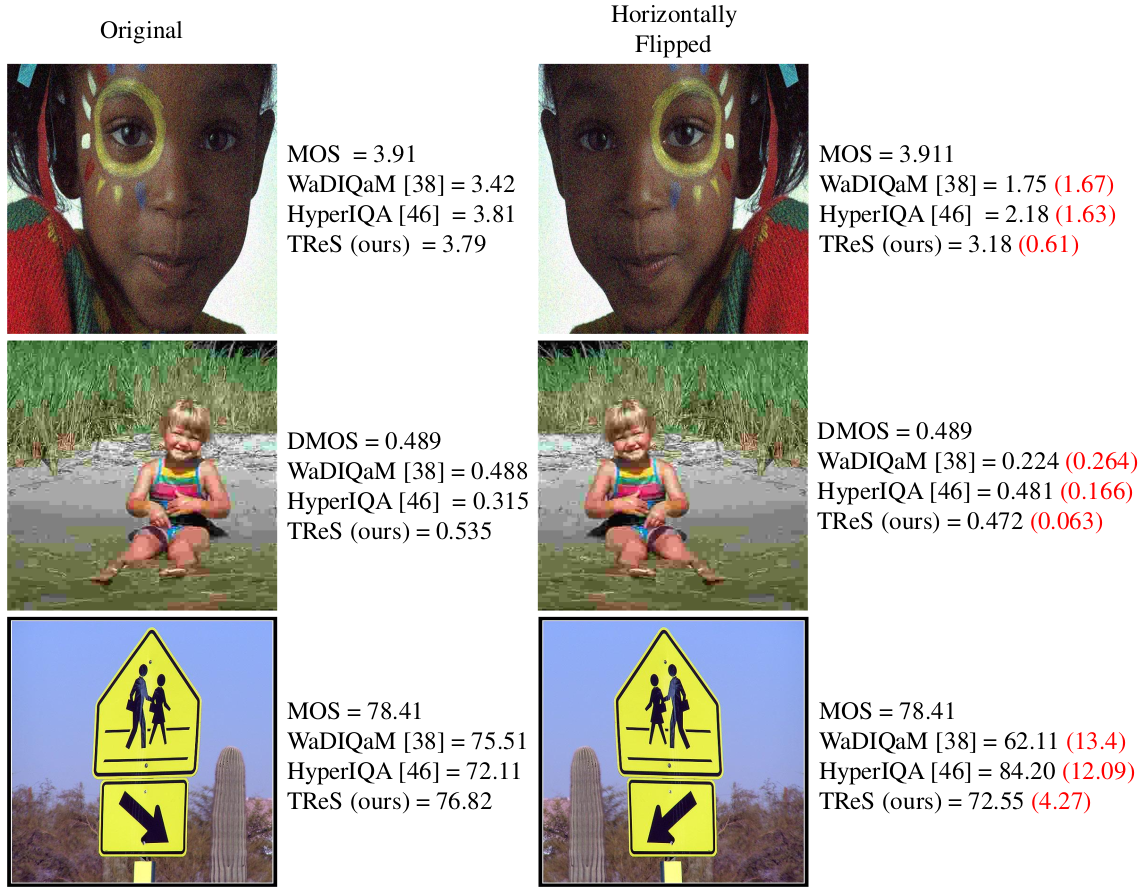
Figure 1: Illustration of the sensitivity of NR-IQA models to horizontal flipping. On the right side of each image, we provide the subjective quality score (MOS/DMOS) and the predicted quality score; the red numbers in the parentheses show the absolute difference between the predictions when the image is flipped.

• We introduce an end-to-end deep learning approach for NR-IQA. Our proposed model utilizes local and non-local information of an image by leveraging CNNs and self-attention mechanism of Transformers. Particularly, in addition to local features that are generated via CNNs, we take advantage of the sequence modeling and self-attention mechanism of Transformers to learn a non-local representation of the image from the multi-scale features that are extracted from different layers of CNNs. The non-local features are then fused with the local features to predict the final image quality score (Sec. 3.1, 3.2, and 3.3).

• We propose a relative ranking loss that explicitly enforces the relative ranking among the samples. We propose to use a triplet loss with an adaptive margin based on the human subjective scores to make the distance between the image with the highest (lowest) quality score closer to the one with the second-highest (second-lowest) quality score and further away from the image with the lowest (highest) score (Sec. 3.4).

• Lastly, we propose to use an equivariant transformation of the input image as a source of self-supervisory to improve the robustness of our proposed model. During the training, we use self-consistency between the output for each image and its transformation to utilize the rich self-supervisory information and reduce the sensitivity of the network (Sec. 3.5).

• Extensive experiments on seven benchmark datasets (for both authentic and synthetic distortions) confirm that our proposed method performs well across different datasets.

2 Related Work

Before the raise of deep learning, early version of general-purpose NR-IQA methods mainly divide into natural scene statistics (NSS) based metrics [16, 17, 6, 5, 18, 19, 8, 20, 21] and learning-based metrics [22, 23, 24, 25, 26, 27]. The underlying assumption for hand-crafted feature-based approaches is that the natural scene statistics (NSS) extracted from natural images are highly regular [28] and different distortions will break such statistical regularities. Variations of NSS features in different domains such as spatial [6, 18, 8], gradient [8], discrete cosine transform (DCT) [5], and wavelet [17], showed impressive performances for synthetically distorted images. Learning-based approaches utilize machine learning techniques such as dictionary learning to map the learned features to the human subjective scores. Ye et al. [23] used a dictionary learning method to encode the raw image patches to features and to predict subjective quality scores by support vector regression (SVR) model. Zhang et al. [26] combined the semantic-level features with local features for quality estimation. Although early versions of hand-crafted and feature learning methods perform well on small synthetically distorted datasets, they suffer from not being able to model real-world distortions.

Deep learning for NR-IQA. By success of deep learning [29, 30] in many computer vision tasks, different approaches utilize deep learning for NR-IQA [31, 32, 33, 34, 35, 36, 37, 38, 39, 36, 40, 41, 42, 43, 10, 44]. Early version of deep learning NR-IQA methods [31, 45, 46, 34, 46, 35] leveraged deep features from CNNs [29, 30] while pretrained on large classification dataset ImageNet [47]. [48, 49] addressed NR-IQA in a multi-task manner where they leverage subjective quality score as well as distortion type simultaneously during the training. Ma et al. [38] proposed a multi-task network where two sub-networks train in two stages for distortion identification and quality prediction. [50, 51, 52, 36] used some sort of the reference images during their training to predicted the quality score in a blind manner. Hallucinated-IQA [36] proposed an NR-IQA method based on generative adversarial models, where they first generated a hallucinated reference image to compensate for the absence of the true reference and then paired the information of hallucinated reference with the distorted image to estimate the quality score. Talebi et al. [37] proposed a CNN-based model to predict the perceptual distribution of subjective quality scores (instead of the mean value). Zhu et al. [43] proposed a model to leverage meta-learning to learn the prior knowledge that is shared among different distortion types. Su et al. [42] proposed a model that extracts content features from the deep model in different scales and pools them to predict image quality.

Transformers for NR-IQA. Currently, CNNs are the main backbone for features extraction among the state-of-the-art NR-IQA models. Although CNNs capture the local structure of the image, they are well known for missing to capture non-local information and having strong locality bias. Furthermore, CNNs demonstrated a bias towards spatial invariance through shared weights across all positions which makes them ineffective if a more complex combination of features is needed. Since IQA highly depends on both local and non-local features, we propose to use Transformers and CNNs together. Inspired by NLP which widely employs Transformers block to model long-range dependencies in language sequence, we utilize a Transformer-based network to compute the dependencies among the CNN extracted features from multi-scales and model the non-local dependency among the extracted features.

Transformers were introduced by Vaswani et al. [53] as a new attention-based building block for machine translation. Attention mechanisms [54] are neural network layers that aggregate information from the entire input sequence. Due to the success of Transformer-based models in the NLP field, we start to see different attempts to explore the benefits of Transformer for computer vision tasks [55, 56, 56, 57, 58, 59]. The application of Transformer for NR-IQA is not explored yet. Concurrently with our work, [60] used Transformers for NR-IQA, where the features from the last layer of CNNs were sent to Transformers for the quality prediction task. Different from [60] that use Transformers as an additional feature extraction block at the end of CNNs, we use it to model the non-local dependency between the extracted multi-scale features. Notably, we leverage the temporal sequence modeling properties of Transformers to compute a non-local representation of the image from the multi-scale features (Sec. 3.2).

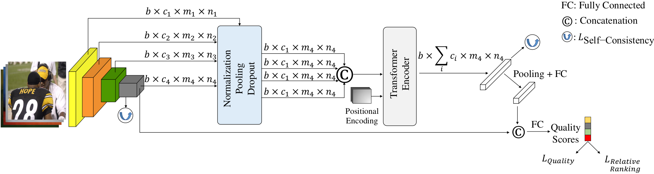
Figure 2: Flowchart of our proposed NR-IQA algorithm.

Learning to rank for NR-IQA. These approaches [61, 62, 38, 39] address NR-IQA as a learning-to-rank problem, where the relative ranking information is used during the training. Zhang et al. [39] leveraged discrete ranking information from images of the same content and distortion but at different levels (degree of distortion) for quality prediction. [63] used continuous ranking information from MOSs and variances between the subjective scores. [38, 64] extracted binary ranking information via FR-IQA methods during the training. However, due to the use of reference images, their method is only applicable to synthetic distortions. Existing ranking-based algorithms use a fixed margin (which is selected empirically) to minimize their losses. Also, most of the aforementioned approaches (except [63]) fails to perform well on the authentic datasets mainly due to the requirement of using referee images during the training stage. In our proposed method, we also leverage the MOS/DMOS information for relative ranking. However, in contrast to the existing methods, we propose to minimize the relative distance among the samples via a triplet loss with an adaptive margin which does not need the empirical margin selection.

Poor generalization in deep neural networks is a well-known problem and an active area of research. In IQA tasks poor generalization is mostly considered as when the model performs well on the dataset that it is trained on but poorly on another dataset with the same type of artifacts. Reasons such as various contents, domain shift, or scale shift in the subjective scores mainly cause the poor generalization of IQA models. In our experiments, in addition to cross dataset evaluation, we also notice that the performance of deep-learning based IQA models degrades when we apply horizontal flipping or rotation to the inputs. Common approaches such as dropout [65], ensembling [66], cross-task consistency [67], and augmentation proposed to increase the generalization in deep models. However, making predictions using a whole ensemble of models is cumbersome and too computationally expensive due to large models’ sizes. Data augmentation has been successful in increasing the generalization of CNNs. However, as shown in Fig. 1, a model can still suffer from poor generalization for a simple transformation. [68, 69] show that although using different augmentation methods improve the generalization of CNNs, they are still sensitive to equivariant perturbations in data.

As shown in Fig. 1, NR-IQA models that used image flipping as an augmentation during training still fail to have a robust quality prediction for an image and its flipped version. This kind of high variance in the quality prediction can affect the robustness of computer vision applications directly. In this work, we improve the consistency of our model via the simple observation that the results of the NR-IQA model should not change under transformations such as horizontal flipping.

3 Proposed Method

In this section, we detail our proposed model, which is an NR-IQA method based on Transformers, Relative ranking, and Self consistency, namely TReS. Fig. 2 shows an overview of our proposed method.

3.1 Feature Extraction

Given an input image $I\in\mathbb{R}^{3\times m\times n}$, where $m$ and $n$ denote width and height, our goal is to estimate its perceptual quality score ($q$). Let $f_{\phi}$ represent a CNN with learnable parameters $\phi$, and $F_{i}\in\mathbb{R}^{b\times c_{i}\times m_{i}\times n_{i}}$ denotes the features from the $i^{th}$ block of CNN, where $i\in\{1,2,3,4\}$, $b$ denotes the batch size, and $c_{i},m_{i}$, and $n_{i}$ denote the channel size, width, and height of the $i^{th}$ feature, respectively. Let $F_{4}\in\mathbb{R}^{b\times c_{4}\times m_{4}\times n_{4}}$ represent the high-level semantic features from the last layer in the $4^{th}$ block of CNN. We use the last layers of each block to extract the multi-scale features from the input image. Since the extracted features from different layers have different ranges, statistics, and dimensions, we first send them to normalization, pooling, and dropout layers. For normalization and pooling we use Euclidean norm which is defined by $F_{i}=\frac{F_{i}}{\max(\left\|F_{i}\right\|_{2},\epsilon)}$ followed by a $\mathit{l}_{2}$ pooling layer [70, 71] which has been used to demonstrate the behavior of complex cells in primary visual cortex [72, 73]. The $\mathit{l}_{2}$ pooling layer defines by:

$$P(x)=\sqrt{g\ast(x\odot x)},$$ (1)

where $\odot$ denotes point-wise product, and the blurring kernel $g(.)$ is implemented via a Hamming window that approximately applies the Nyquist criterion [71]. Let $\bar{F}_{i}\in\mathbb{R}^{b\times c_{i}\times m_{4}\times n_{4}}$ denote the output feature after sending $F_{i}$ to the normalization, pooling, and dropout layers. Next, we concatenate $\bar{F}_{i}$, where $i\in\{1,2,3,4\}$, and denote the output by $\tilde{F}\in\mathbb{R}^{b\times\sum_{i}c_{i}\times m_{4}\times n_{4}}$.

3.2 Attention-Based Feature Computation

CNNs exploit the structure of images via local interactions through convolution with small kernel sizes. Different layers of a network can have different semantic information that is captured through the local interactions, and as we move from lower layers to the higher layers, the computed features carry more semantic about the content of the image [74]. IQA depends on both low- and high-level features. A model that does not take into account both low- and high-level features can mistake a plain sky as a low-quality image [15]. Moreover, due to the architecture of CNNs they mainly capture the local spatial structure of the image and are unable to model the relation among the non-local features.

Transformers have shown impressive results in modeling the dependencies among the sequential data. Therefore, we use the encoder part of the Transformer, which is composed of a multi-head self-attention layer and a feed-forward neural network [75, 53, 59] to perform attention operations over the multi-scale extracted features from different layers and model the dependencies among them. We follow the encoder architecture of [59] (see Fig. 3). We model the features from different layers of CNN as a sequence of information ($\tilde{F}$) and send them to the Transformer encoder. Since the self-attention mechanism is a non-local operation, we use it to compute a non-local representation of the image. In other words, we use Transformers to compute information for each element of extracted features with respect to the others (not only the local neighbor features). Transformer architecture contains no built-in inductive prior to the locality of interactions and, is free to learn complex relationships across the features. We also add positional encoding (in a similar way as [76, 77]) to the input of the attention layers to deal with the permutation-invariant property of Transformers. The positional encoding will also let our model be aware of the position of the features that contribute the most to the IQA task.

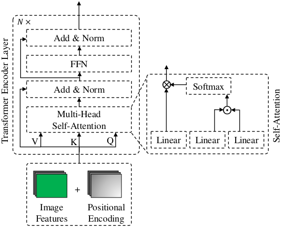
Figure 3: Illustration of multi-head multi-layer self-attention module of the Transformer Encoder layer. $N$ is a hyperparameter that denotes the number of encoder layers In the Transformer which stack together.

In detail, given an input ($\tilde{F}$) and the number of heads ($\mathit{h}$), the input is first transformed into three different groups of vectors, the query group, the key group and the value group. Given a multi-head attention module with $\mathit{h}$ heads and dimension of $d$, each of the aforementioned groups will have dimension of $d^{{}^{\prime}}=\frac{d}{h}$. Then, features derived from different inputs are packed together into three different groups of matrices $Q^{\prime},K^{\prime},$ and $V^{\prime}$, where $Q^{\prime}=\{Q_{i}\}_{i=1}^{h}=Concat(Q_{1},...,Q_{h})$ and the same definition applies to $K^{\prime}$ and $V^{\prime}$. Next, the process of multi-head attention is computed as follows:

where $\mathit{W_{1}}$ is the linear projection matrix and has dimension of $d\times d$, ${head}_{i}={Attention}(Q_{i},K_{i},V_{i}),$ and $Attention(Q,K,V)=softmax(\frac{QK^{T}}{\sqrt{d^{\prime}}})\odot V$. For the first Transformer encoder layer, the query, key, and value matrices ($Q$, $K$, and $V$) are all the same. Following the encoder architecture design in [53], to strengthen the flow of information and improve the performance, a residual connection followed by a layer normalization is added in each sub-layer in the encoder. Next, a feed-forward network (FNN) is applied after the self-attention layers [53]. FNN is consist of two linear transformation layers and a ReLU activation function within them, which can be denoted as $FFN(X)={W_{3}}\sigma({W_{2}}X+b^{\prime}_{2})+b^{\prime}_{3}$, where $\mathit{W_{2}}$ and $\mathit{W_{3}}$ are the two parameter matrices, and $b^{\prime}_{2}$ and $b^{\prime}_{3}$ are the biases. $\sigma$ represents the ReLU activation function. Let $\hat{F}\in\mathbb{R}^{b\times\sum_{i}^{4}c_{i}\times m_{4}\times n_{4}}$ represent the output features from the final Transformer encoder layer.

3.3 Feature Fusion and Quality Prediction

To benefit from the extracted features from both local (convolution) and non-local (self-attention) operators we use fully connected (FC) layers as fusion layers to map the aforementioned features and predict the perceptual quality of the image (see Fig. 2). For each batch of images, $B$, we minimize the regression loss to train our network.

where $q_{i}$ is the predicted quality score for $i^{th}$ image and $s_{i}$ is its corresponding ground truth (subjective quality score).

3.4 Relative Ranking

Although the regression loss (Eq. 3) is effective for the quality prediction task, it does not explicitly take into account ranking and correlation among images. Here, our goal is to consider the relative ranking relation between the samples within each batch. It is computationally expensive to consider all the samples’ relative ranking information; therefore, we only enforce it for the extreme cases. Among images within the batch $B$, let $q_{max},q^{\prime}_{max},q_{min},$ and $q^{\prime}_{min}$ denote the predicted quality for images with highest, second highest, lowest, and second lowest subjective quality scores, respectively, i.e., $s_{q_{max}}>s_{q^{\prime}_{max}}>s_{q^{\prime}_{min}}>s_{q_{min}}$, where $s_{q_{max}}$ denotes the subjective quality score corresponding to the image with the predicted quality score $q_{max}$, and a similar notation rule applies to the rest. Our goal is to have $d(q_{max},q^{\prime}_{max})+margin_{1}\leq d(q_{max},q_{min})$, here we define, $d(x,y)$ as the absolute value between $x$ and $y$, $d(x,y)=\mathinner{\!\left\lvert x-y\right\rvert}$. We utilize triplet loss to address the above inequality, where we minimize $\max\{0,d(q_{max},q^{\prime}_{max})-d(q_{max},q_{min})+margin_{1}\}$. In a similar way, we also want to have $d(q_{min},q^{\prime}_{min})+margin_{2}\leq d(q_{max},q_{min})$. The $margin$ values can be selected empirically based on each dataset, but that is cumbersome since each dataset have different distributions and ranges for the quality scores. For a perfect prediction where the estimated quality scores are the same as subjective scores we will have $margin_{1}+\mathinner{\!\left\lvert s_{q_{max}}-s_{q^{\prime}_{max}}\right\rvert}\leq\mathinner{\!\left\lvert s_{q_{max}}-s_{q_{min}}\right\rvert}\rightarrow margin_{1}+(s_{q_{max}}-s_{q^{\prime}_{max}})\leq(s_{q_{max}}-s_{q_{min}})\rightarrow margin_{1}\leq s_{q^{\prime}_{max}}-s_{q_{min}}.$ Therefore, we can consider $s_{q^{\prime}_{max}}-s_{q_{min}}$ to be an upper-bound for $margin_{1}$ during the training, and set $margin_{1}=s_{q^{\prime}_{max}}-s_{q_{min}}$ in Eq. 4. Similarly, we define $margin_{2}=s_{q_{max}}-s^{\prime}_{q_{min}}$. Finally, our relative ranking loss is defined as:

$$\mathcal{L}_{Relative-Ranking,B}=$$ (4)

$$\mathcal{L}_{triplet}(q_{max},q^{\prime}_{max},q_{min})+\mathcal{L}_{triplet}(q_{min},q^{\prime}_{min},q_{max})$$

$$=\max\{0,d(q_{max},q^{\prime}_{max})-d(q_{max},q_{min})+margin_{1}\}$$

$$+\max\{0,d(q^{\prime}_{min},q_{min})-d(q_{max},q_{min})+margin_{2}\}.$$

3.5 Self-Consistency

Last but not least, we propose to utilize the model’s uncertainty for the input image and its equivariant transformation during the training process. We exploit self-consistency via the self-supervisory signal between each image and its equivariant transformation to increase the robustness of the model. Let for an input $I$, $f_{\phi,conv}(I)$ and $f_{\theta,atten}(I)$ denote the output logits belonging to outputs of the convolution and Transformer layers, respectively, where $f_{\phi,conv}$ and $f_{\theta,atten}$ represent the CNN and Transformer with learnable parameters $\phi$ and $\theta$, respectively. In our model, we use the outputs of $f_{\phi,conv}$ and $f_{\theta,atten}$ to predict the image quality and since the human subjective scores stay the same for the horizontal filliping version of the input image, we thus expect to have $f_{\phi,conv}(I)=f_{\phi,conv}(\tau(I))$ and $f_{\theta,atten}(I)=f_{\theta,atten}(\tau(I))$, where $\tau$ represents the horizontal filliping transformation. In this way, by applying our consistency loss, the network learns to reinforce representation learning of itself without additional labels and external supervision. We minimize the self-consistency loss that is defined as follows:

$$\mathcal{L}_{Self-Consistency}=$$ (5)

$$\left\|f_{\phi,conv}(I)-f_{\phi,conv}(\tau(I))\right\|+$$

$$\left\|f_{\theta,atten}(I)-f_{\theta,atten}(\tau(I))\right\|+$$

$$\lambda_{1}\left\|\mathcal{L}_{Relative-Ranking,B}-\mathcal{L}_{Relative-Ranking,\tau(B)}\right\|,$$

where $\tau(B)$ denote when the equivariant transformation applies on batch $B$.

3.6 Losses

Our model trains in an end-to-end manner and minimizes the aforementioned losses together simultaneously. The total loss for our model is defined as:

$$\begin{array}[]{lll}\mathcal{L}_{total}&=\mathcal{L}_{Quality}+\lambda_{2}\mathcal{L}_{Relative-Ranking}+\\ &\lambda_{3}\mathcal{L}_{Self-Consistency},\end{array}$$ (6)

where $\lambda_{1},\lambda_{2},\lambda_{3}$ are balancing coefficients.

4 Experiments

4.1 Datasets and Evaluation Metrics

We evaluate the performance of our proposed model extensively on seven publicly available IQA datasets (four synthetically distorted and three authentically distorted). For synthetically distorted datasets, we use LIVE [78], CSIQ [79], TID2013 [80], and KADID-10K [81], where among them KADID has the most number of distortion typesand distorted images. For authentically distorted datasets, we use CLIVE [9], KonIQ-10k [10], and LIVE-FB [11], where among them LIVE-FB has the most number of unique contents. Table 1 shows the summary of the datasets that are used in our experiments.

Table 1: Summary of IQA datasets.

Databases	# of Dist.	# of Dist.	Distortions
	Images	Types	Type
LIVE	799	5	synthetic
CSIQ	866	6	synthetic
TID2013	3,000	24	synthetic
KADID	10,125	25	synthetic
CLIVE	1,162	-	authentic
KonIQ	10,073	-	authentic
LIVEFB	39,810	-	authentic

Table 2: Comparison of TReS v.s. state-of-the-art NR-IQA algorithms on synthetically and authentically distorted datasets. Bold entries in black and blue are the best and second-best performers, respectively. * code were not available publicly.

	LIVE		CSIQ		TID2013		KADID		CLIVE		KonIQ		LIVEFB		Weighted Average
	PLCC	SROCC	PLCC	SROCC	PLCC	SROCC	PLCC	SROCC	PLCC	SROCC	PLCC	SROCC	PLCC	SROCC	PLCC	SROCC
HFD*[82]	0.971	0.951	0.890	0.842	0.681	0.764	-	-	-	-	-	-	-	-	-	-
PQR*[35]	0.971	0.965	0.901	0.873	0.864	0.849	-	-	0.836	0.808	-	-	-	-	-	-
DIIVINE[5]	0.908	0.892	0.776	0.804	0.567	0.643	0.435	0.413	0.591	0.588	0.558	0.546	0.187	0.092	0.323	0.264
BRISQUE[6]	0.944	0.929	0.748	0.812	0.571	0.626	0.567	0.528	0.629	0.629	0.685	0.681	0.341	0.303	0.457	0.430
ILNIQE[8]	0.906	0.902	0.865	0.822	0.648	0.521	0.558	0.534	0.508	0.508	0.537	0.523	0.332	0.294	0.430	0.394
BIECON[83]	0.961	0.958	0.823	0.815	0.762	0.717	0.648	0.623	0.613	0.613	0.654	0.651	0.428	0.407	0.527	0.507
MEON[38]	0.955	0.951	0.864	0.852	0.824	0.808	0.691	0.604	0.710	0.697	0.628	0.611	0.394	0.365	0.514	0.479
WaDIQaM[34]	0.955	0.960	0.844	0.852	0.855	0.835	0.752	0.739	0.671	0.682	0.807	0.804	0.467	0.455	0.595	0.584
DBCNN[39]	0.971	0.968	0.959	0.946	0.865	0.816	0.856	0.851	0.869	0.869	0.884	0.875	0.551	0.545	0.679	0.671
TIQA[60]	0.965	0.949	0.838	0.825	0.858	0.846	0.855	0.850	0.861	0.845	0.903	0.892	0.581	0.541	0.698	0.670
MetaIQA[43]	0.959	0.960	0.908	0.899	0.868	0.856	0.775	0.762	0.802	0.835	0.856	0.887	0.507	0.540	0.634	0.656
P2P-BM[11]	0.958	0.959	0.902	0.899	0.856	0.862	0.849	0.840	0.842	0.844	0.885	0.872	0.598	0.526	0.705	0.658
HyperIQA[42]	0.966	0.962	0.942	0.923	0.858	0.840	0.845	0.852	0.882	0.859	0.917	0.906	0.602	0.544	0.715	0.676
TReS (proposed)	0.968	0.969	0.942	0.922	0.883	0.863	0.858	0.859	0.877	0.846	0.928	0.915	0.625	0.554	0.732	0.685

For performance evaluation, we employ two commonly used criteria, namely Spearman’s rank-order correlation coefficient (SROCC) and Pearson’s linear correlation coefficient (PLCC). Both SROCC and PLCC range from 0 to 1, and a higher value indicates a better performance. Following Video Quality Expert Group (VQEG) [84], for PLCC, logistic regression is first applied to remove nonlinear rating caused by human visual observation.

4.2 Implementation Details

We implemented our model by PyTorch and conducted training and testing on an NVIDIA RTX 2080 GPU. Following the standard training strategy from existing IQA algorithms, we randomly select multiple sample patches from each image and horizontally and vertically augment them randomly. Particularly, we select 50 patches randomly with the size of $224\times 224$ pixels from each training image. Training patches inherited quality scores from the source image, and we minimize $\mathcal{L}_{total}$ loss over the training set. We used Adam [85] optimizer with weight decay $5\times 10^{-4}$ to train our model for at most 5 epochs, with mini-batch size of 53. The learning rate is first set to $2\times 10^{-5}$ and reduced by $10$ after every epoch. During the testing stage, 50 patches with $224\times 224$ pixels from the test image are randomly sampled, and their corresponding prediction scores are average pooled to get the final quality score. We use ResNet50 [30] for our CNN backbone unless mentioned otherwise, while it is initialized with Imagenet weights. We use $N=2$ for number of encoder layers in the Transformer, $d=64$, and set the number of heads $h=16$. The hyper parameters $\lambda_{1},\lambda_{2},\lambda_{3}$ are empirically set to $0.5,0.05,1$, respectively.

Following the common practice in NR-IQA, all experiments use the same setting, where we first select $10$ different seeds, and then use them to split the datasets randomly to train/test ($80\%/20\%$), so we have $10$ different splits. Testing data is not being used during the training. In the case of synthetically distorted datasets, the split is implemented according to reference images to avoid content overlapping. For all of the reported results we run the experiment $10$ times with different initialization and report the median SROCC and PLCC values.

4.3 Performance Evaluation

Table 2 shows the overall performance comparison in terms of PLCC and SROCC on seven standard image quality datasets, which cover both synthetically and authentically distorted images. Furthermore, our model outperforms the existing methods by a significant margin on both LIVEFB and KADID datasets that are currently the largest datasets for in-the-wild images and synthetically distorted images, respectively. Our model also achieves competitive results on the smaller datasets. In the last column, we provide the weighted average performance across all datasets, using the dataset sizes as weights for the performances, and we observe that our proposed method outperforms existing methods on both PLCC and SROCC.

In Table 3, we conduct cross dataset evaluations and compare our model to the competing approaches. Training is performed on one specific dataset, and testing is performed on a different dataset without any finetuning or parameter adaptation. For synthetic image datasets (LIVE, CSIQ, TID2013), we select four distortion types (i.e., JPEG, JPEG2K, WN, and Blur) which all the datasets have in common. As shown in Table 3, our proposed method outperforms other algorithms on four datasets among six, which indicate the strong generalization power of our approach.

Table 3: SROCC evaluations on cross datasets, where bold entries indicate the best performers.

Train on	LIVEFB		CLIVE	KonIQ	LIVE
Test on	KonIQ	CLIVE	KonIQ	CLIVE	CSIQ	TID2013
WaDIQaM[34]	0.708	0.699	0.711	0.682	0.704	0.462
DBCNN[39]	0.716	0.724	0.754	0.755	0.758	0.524
P2P-BM[11]	0.755	0.738	0.740	0.770	0.712	0.488
HyperIQA[42]	0.758	0.735	0.772	0.785	0.744	0.551
TReS (Proposed)	0.713	0.740	0.733	0.786	0.761	0.562

We evaluate the latent features learned by our model in Fig. 4, where we use the latent features from the last layer of the network for query images and collect the top three nearest neighbor results for the corresponding query. As shown in Fig. 4, although we do not explicitly model the content or distortion types in our model, the nearest neighbor samples have similar content or artifacts in terms of perceptual quality and have close subjective scores to each other, which represent the effectiveness of our model in terms of feature representation. Specifically, in the first row, our model selects images with the same motion blur artifacts as the nearest neighbor samples. In the second row, our model selects images with low lighting condition which follow similar quality conditions as the query image.

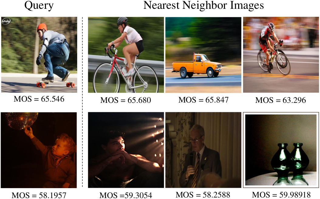
Figure 4: Nearest neighbor retrieval results. In each row, the leftmost image is a query image, and the rest are the top 3 nearest neighbors, using the latent features learned by our proposed models. The nearest neighbor retrieval process is done on the test portion of the datasets. Images in the first and second rows are taken from the LIVEFB dataset.

Moreover, in Fig. 5, we show the spatial quality map generated from the layer with the highest activation in our model. The bright regions represent the poor quality regions in the input images.

4.4 Ablation Study

In Table 4, we provide ablation experiments to illustrate the effect of each component of our proposed method by comparing the results on KADID and KonIQ datasets. Furthermore, in Table 5, we evaluate the performance sensitivity of our model for smaller backbones. For a fair comparison to existing algorithms, we chose Resnet50 for all of the experiments in this paper. However, as shown in Table 5, for smaller backbones, our model still achieves comparable results. As shown in Table 5, for large datasets (e.g., LIVEFB or KonIQ), the performance of our model does not drop significantly and is still competitive when we use a smaller backbone, which demonstrates the learning capacity of our proposed model.

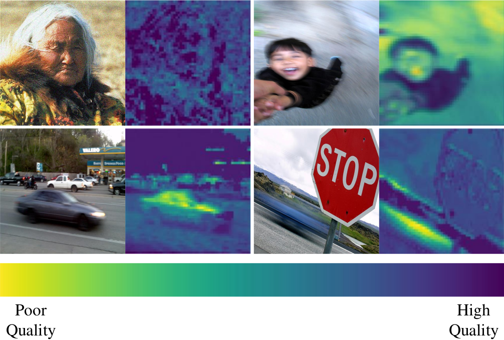
Figure 5: Spatial quality maps generated using the our proposed model. Left: Original Images. Right: Quality maps blended with the originals using viridis color.

Table 4: Ablation experiments on the effects of different components for our proposed model.

Resnet50	Transformer	Psitional	Relative	Self	KADID		KonIQ
		Encoding	Ranking	Consistency	PLCC	SROCC	PLCC	SROCC
✓					0.809	0.802	0.873	0.851
✓			✓	✓	0.822	0.820	0.896	0.884
✓	✓				0.833	0.820	0.886	0.872
✓	✓	✓			0.840	0.832	0.902	0.0.895
✓	✓	✓	✓		0.851	0.850	0.918	0.911
✓	✓	✓	✓	✓	0.858	0.859	0.928	0.915

Table 5: Ablation experiments on the performance of our proposed model via different backbones.

Dataset	Backbone	PLCC	SROCC	Dataset	Backbone	PLCC	SROCC
CLIVE	Resnet-50	0.877	0.846	CSIQ	Resnet-50	0.942	0.922
	Resnet-34	0.855	0.830		Resnet-34	0.924	0.920
	Resnet-18	0.859	0.822		Resnet-18	0.911	0.914
KonIQ	Resnet-50	0.928	0.915	TID2013	Resnet-50	0.883	0.863
	Resnet-34	0.922	0.909		Resnet-34	0.847	0.813
	Resnet-18	0.909	0.898		Resnet-18	0.843	0.810
LIVEFB	Resnet-50	0.625	0.560	KADID	Resnet-50	0.858	0.859
	Resnet-34	0.619	0.554		Resnet-34	0.851	0.855
	Resnet-18	0.611	0.550		Resnet-18	0.840	0.848

4.5 Failure Cases and Discussion

In Fig. 6, we show examples where our method fails to predict the image quality in agreement with the human subjective scores. All images in Fig. 6 have close ground truth scores, and our model predicted different scores for each image. From the modeling aspect, we think one reason for such a failure is that IQA models have to address the IQA task as either a regression and/or classification problem (simply because the existing datasets provide only the quality score(s) for each image). Recently, LIVEFB [11] provides patch-wise quality scores for local patches of each image and shows that incorporating patch scores leads to better performance. As a future direction, we think what is missing from the existing IQA datasets is a description of the reasoning process from the subjects to explain the reason behind their selected quality score; this can help the future models be able to model the HVS and reasoning behind the assigned quality scores in a better way for a more precise perceptual quality assessment. On the other hand, from the subjective scores perspective, the subjects may be less forgiving of the blur artifact and grayscale images, so those artifacts have drawn their attentions similarly. However, our model differentiates between different perceptual cues (color, sharpness, blurriness), which can explain the differences in the scores.

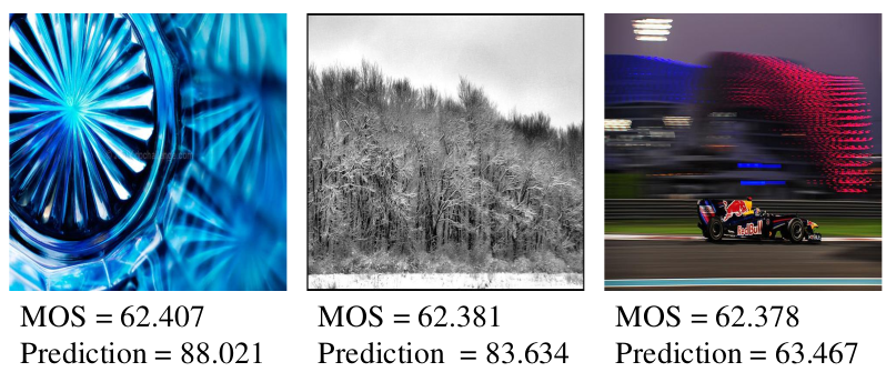
Figure 6: Failure cases, where the predictions are different from the subjective scores (MOS).

5 Conclusion

In this work, we present an NR-IQA algorithm that works based on a hybrid combination of CNNs and Transformers features to utilize both local and non-local feature representation of the input image. We further propose a relative ranking loss that takes into account the relative ranking information among the images. Finally, we exploit an additional self-consistency loss to improve the robustness of our proposed method. Our experiments show that our proposed method performs well on several IQA datasets covering synthetically and authentically distorted images.

Fig. 7 shows the scatter plots of our model’s predictions v.s. subjective ratings (MOS/DMOS) for all seven datasets. As shown in Fig. 7, the recently proposed FBLIVE dataset is the most challenging one. Although we achieve state-of-the-art on FBLIVE dataset comparing to existing algorithms, there is still a long way to go for understanding how the human vision system evaluates the quality of images in-the-wild.

A fair question is why not using other types of transformation instead of horizontal flipping and how they will affect the performance if we use them for self-consistency. In Table 6, we provide an ablation study where we consider other types of transformations to enforce self-consistency.

Table 6: SROCC results for ablation study for different equivariant transformations for the self-consistency loss.

Components	KADID	KonIQ
Baseline	0.850	0.911
Horizontal Flipping	0.859	0.915
Vertical Flipping	0.852	0.882
Rotation 90 Degree	0.851	0.891
Random Translation 16-20 pixels	0.854	0.913
Random Crop	0.832	0.872
Horizontal Flipping + Translation	0.860	0.916

Based on our experiments, for synthetically distorted datasets horizontal and vertical flipping, rotation, and translation can also improve the performance. For authentically distorted datasets we observe that only horizontal flipping and translation yield performance improvement. These experiments can explain that for synthetic datasets the artifacts play an important role and different transformations can help the model captures the artifacts better and become independent of the content information. However, for authentic quality assessment, the quality score is a combination of different factors and therefore some of the transformations can hurt the performance instead of helping. For example, to a viewer, a rotated version of the image will not have the same authentic quality score as the original one, therefore, enforcing the self-consistency would not be beneficial.

Also, we would like to emphasize that although our self-consistency will not add any computation to the interface time, it will require more GPU memory during the training, therefore it will be computationally expensive to apply multiple transformations at the same time. Nonetheless, in the last row of Table 6, we show that a combination of horizontal flipping and translation can further improve the results. As future work, we would like to consider improving the computational complexity of our self-consistency idea.

Last but not least, we claim in the paper that the features generated from CNNs and Transformers represent two different aspects of an image. In Fig. 7, we visualize the features of the last layer of our CNN model (second column) and our Transformer model (third column) for images with the same content but different artifacts. We can observe that for each image the CNN features and Transformer features represent completely different information. Moreover, we can observe that the features from the CNN (or Transformer) layer for different artifacts are also different, which proves the power of our model in capturing different informative information for each image.

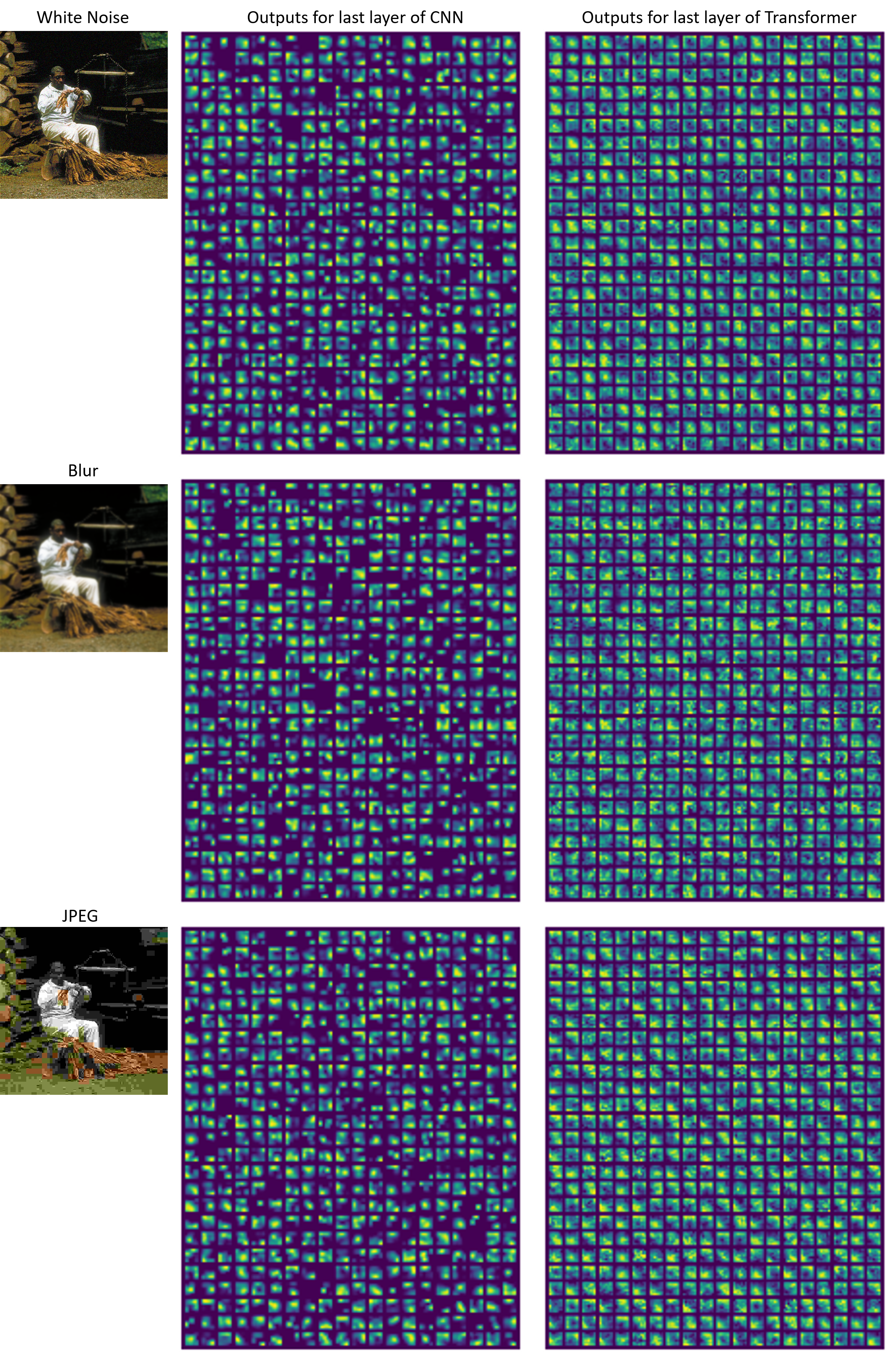
Figure 7: Visualization of features from the last layer of CNN and Transformer. Our CNN and Transformer models capture different information for each image as well as across different distortion types.

FQAs

1) What is the difference between self-consistency and ensembling? and will the self-consistency increase the interface time? In ensampling methods, we need to have several models (with different initializations) and ensemble the results during the training and testing, but in our self-consistency model, we enforce one model to have consistent performance for one network during the training while the network has an input with different transformations. Our self-consistency model has the same interface time/parameters in the testing similar to the model without self-consistency. In other words, we are not adding any new parameters to the network and it won’t affect the interface.

2) What is the difference between self-consistency and augmentation? In augmentation, we augment an input and send it to one network, so although the network will become robust to different augmentation, it will never have the chance of enforcing the outputs to be the same for different versions of an input at the same time. In our self-consistency approach, we force the network to have a similar output for an image with a different transformation (in our case horizontal flipping) which leads to more robust performance. Please also note that we still use augmentation during the training, so our model is benefiting from the advantages of both augmentation and self-consistency. Also, please see Fig. 1 in the main paper, where we showed that models that used augmentation alone are sensitive to simple transformations.

3) Why does the relative ranking loss apply to the samples with the highest and lowest quality scores, why not applying it to all the samples? 1) We did not see a significant improvement by applying our ranking loss to all the samples within each batch compared to the case that we just use extreme cases. 2) Considering more samples lead to more gradient back-propagation and therefore more computation during the training which causes slower training.

References

- [1] Y. Lou, Y. Bai, J. Liu, S. Wang, and L. Duan, “Veri-wild: A large dataset and a new method for vehicle re-identification in the wild,” in Proceedings of the IEEE Conference on Computer Vision and Pattern Recognition, 2019.
- [2] T.-Y. Chiu, Y. Zhao, and D. Gurari, “Assessing image quality issues for real-world problems,” in Proceedings of the IEEE Conference on Computer Vision and Pattern Recognition, 2020.
- [3] Z. Zhu, D. Liang, S. Zhang, X. Huang, B. Li, and S. Hu, “Traffic-sign detection and classification in the wild,” in Proceedings of the IEEE conference on computer vision and pattern recognition, 2016.
- [4] Z. Wang and A. C. Bovik, “Modern image quality assessment,” Synthesis Lectures on Image, Video, and Multimedia Processing, vol. 2, 2006.
- [5] M. A. Saad, A. C. Bovik, and C. Charrier, “Blind image quality assessment: A natural scene statistics approach in the dct domain,” IEEE transactions on Image Processing, vol. 21, no. 8, 2012.
- [6] A. Mittal, A. K. Moorthy, and A. C. Bovik, “No-reference image quality assessment in the spatial domain,” IEEE Transactions on image processing, vol. 21, no. 12, pp. 4695–4708, 2012.
- [7] W. Xue, L. Zhang, and X. Mou, “Learning without human scores for blind image quality assessment,” in Proceedings of the IEEE Conference on Computer Vision and Pattern Recognition, 2013.
- [8] L. Zhang, L. Zhang, and A. C. Bovik, “A feature-enriched completely blind image quality evaluator,” IEEE Transactions on Image Processing, vol. 24, no. 8, pp. 2579–2591, 2015.
- [9] D. Ghadiyaram and A. C. Bovik, “Massive online crowdsourced study of subjective and objective picture quality,” IEEE Transactions on Image Processing, vol. 25, 2015.
- [10] V. Hosu, H. Lin, T. Sziranyi, and D. Saupe, “Koniq-10k: An ecologically valid database for deep learning of blind image quality assessment,” IEEE Transactions on Image Processing, vol. 29, 2020.
- [11] Z. Ying, H. Niu, P. Gupta, D. Mahajan, D. Ghadiyaram, and A. Bovik, “From patches to pictures (paq-2-piq): Mapping the perceptual space of picture quality,” in Proceedings of the IEEE Conference on Computer Vision and Pattern Recognition, IEEE, 2020.
- [12] C.-H. Chou and Y.-C. Li, “A perceptually tuned subband image coder based on the measure of just-noticeable-distortion profile,” IEEE Transactions on circuits and systems for video technology, vol. 5, 1995.
- [13] Z. Wang and A. C. Bovik, “Mean squared error: Love it or leave it? a new look at signal fidelity measures,” IEEE signal processing magazine, vol. 26, no. 1, 2009.
- [14] M. M. Alam, K. P. Vilankar, D. J. Field, and D. M. Chandler, “Local masking in natural images: A database and analysis,” Journal of vision, vol. 14, 2014.
- [15] D. Li, T. Jiang, W. Lin, and M. Jiang, “Which has better visual quality: The clear blue sky or a blurry animal?,” IEEE Transactions on Multimedia, vol. 21, no. 5, 2018.
- [16] A. K. Moorthy and A. C. Bovik, “A two-step framework for constructing blind image quality indices,” IEEE Signal processing letters, vol. 17, no. 5, 2010.
- [17] A. K. Moorthy and A. C. Bovik, “Blind image quality assessment: From natural scene statistics to perceptual quality,” IEEE transactions on Image Processing, vol. 20, no. 12, pp. 3350–3364, 2011.
- [18] A. Mittal, R. Soundararajan, and A. C. Bovik, “Making a “completely blind” image quality analyzer,” IEEE Signal processing letters, vol. 20, no. 3, pp. 209–212, 2012.
- [19] X. Gao, F. Gao, D. Tao, and X. Li, “Universal blind image quality assessment metrics via natural scene statistics and multiple kernel learning,” IEEE Transactions on neural networks and learning systems, vol. 24, no. 12, 2013.
- [20] J. Xu, P. Ye, Q. Li, H. Du, Y. Liu, and D. Doermann, “Blind image quality assessment based on high order statistics aggregation,” IEEE Transactions on Image Processing, vol. 25, no. 9, pp. 4444–4457, 2016.
- [21] D. Ghadiyaram and A. C. Bovik, “Perceptual quality prediction on authentically distorted images using a bag of features approach,” Journal of vision, vol. 17, no. 1, 2017.
- [22] P. Ye and D. Doermann, “No-reference image quality assessment using visual codebooks,” IEEE Transactions on Image Processing, vol. 21, no. 7, 2012.
- [23] P. Ye, J. Kumar, L. Kang, and D. Doermann, “Unsupervised feature learning framework for no-reference image quality assessment,” in Proceedings of the IEEE Conference on Computer Vision and Pattern Recognition, IEEE, 2012.
- [24] L. Zhang, Z. Gu, X. Liu, H. Li, and J. Lu, “Training quality-aware filters for no-reference image quality assessment,” IEEE MultiMedia, vol. 21, 2014.
- [25] P. Ye, J. Kumar, and D. Doermann, “Beyond human opinion scores: Blind image quality assessment based on synthetic scores,” in Proceedings of the IEEE Conference on Computer Vision and Pattern Recognition, pp. 4241–4248, 2014.
- [26] P. Zhang, W. Zhou, L. Wu, and H. Li, “Som: Semantic obviousness metric for image quality assessment,” in Proceedings of the IEEE Conference on Computer Vision and Pattern Recognition, pp. 2394–2402, 2015.
- [27] K. Ma, W. Liu, T. Liu, Z. Wang, and D. Tao, “dipiq: Blind image quality assessment by learning-to-rank discriminable image pairs,” IEEE Transactions on Image Processing, vol. 26, no. 8, pp. 3951–3964, 2017.
- [28] E. P. Simoncelli and B. A. Olshausen, “Natural image statistics and neural representation,” Annual review of neuroscience, vol. 24, no. 1, pp. 1193–1216, 2001.
- [29] A. Krizhevsky, I. Sutskever, and G. E. Hinton, “Imagenet classification with deep convolutional neural networks,” Advances in neural information processing systems, vol. 25, 2012.
- [30] K. He, X. Zhang, S. Ren, and J. Sun, “Deep residual learning for image recognition,” in Proceedings of the IEEE conference on computer vision and pattern recognition, pp. 770–778, 2016.
- [31] L. Kang, P. Ye, Y. Li, and D. Doermann, “Convolutional neural networks for no-reference image quality assessment,” in Proceedings of the IEEE conference on computer vision and pattern recognition, pp. 1733–1740, 2014.
- [32] J. Long, E. Shelhamer, and T. Darrell, “Fully convolutional networks for semantic segmentation,” in Proceedings of the IEEE conference on computer vision and pattern recognition, pp. 3431–3440, 2015.
- [33] J. Redmon, S. Divvala, R. Girshick, and A. Farhadi, “You only look once: Unified, real-time object detection,” in Proceedings of the IEEE conference on computer vision and pattern recognition, 2016.
- [34] S. Bosse, D. Maniry, K.-R. Müller, T. Wiegand, and W. Samek, “Deep neural networks for no-reference and full-reference image quality assessment,” IEEE Transactions on Image Processing, vol. 27, 2017.
- [35] H. Zeng, L. Zhang, and A. C. Bovik, “A probabilistic quality representation approach to deep blind image quality prediction,” arXiv preprint arXiv:1708.08190, 2017.
- [36] K.-Y. Lin and G. Wang, “Hallucinated-iqa: No-reference image quality assessment via adversarial learning,” in Proceedings of the IEEE Conference on Computer Vision and Pattern Recognition, pp. 732–741, 2018.
- [37] H. Talebi and P. Milanfar, “Nima: Neural image assessment,” IEEE Transactions on Image Processing, vol. 27, no. 8, pp. 3998–4011, 2018.
- [38] K. Ma, W. Liu, K. Zhang, Z. Duanmu, Z. Wang, and W. Zuo, “End-to-end blind image quality assessment using deep neural networks,” IEEE Transactions on Image Processing, vol. 27, no. 3, pp. 1202–1213, 2017.
- [39] W. Zhang, K. Ma, J. Yan, D. Deng, and Z. Wang, “Blind image quality assessment using a deep bilinear convolutional neural network,” IEEE Transactions on Circuits and Systems for Video Technology, vol. 30, 2018.
- [40] S. Bianco, L. Celona, P. Napoletano, and R. Schettini, “On the use of deep learning for blind image quality assessment,” Signal, Image and Video Processing, vol. 12, no. 2, 2018.
- [41] B. Yan, B. Bare, and W. Tan, “Naturalness-aware deep no-reference image quality assessment,” IEEE Transactions on Multimedia, vol. 21, no. 10, pp. 2603–2615, 2019.
- [42] S. Su, Q. Yan, Y. Zhu, C. Zhang, X. Ge, J. Sun, and Y. Zhang, “Blindly assess image quality in the wild guided by a self-adaptive hyper network,” in Proceedings of the IEEE Conference on Computer Vision and Pattern Recognition, pp. 3667–3676, 2020.
- [43] H. Zhu, L. Li, J. Wu, W. Dong, and G. Shi, “Metaiqa: deep meta-learning for no-reference image quality assessment,” in Proceedings of the IEEE Conference on Computer Vision and Pattern Recognition, 2020.
- [44] W. Zhang, K. Zhai, G. Zhai, and X. Yang, “Learning to blindly assess image quality in the laboratory and wild,” in 2020 IEEE International Conference on Image Processing, pp. 111–115, IEEE, 2020.
- [45] S. Bosse, D. Maniry, T. Wiegand, and W. Samek, “A deep neural network for image quality assessment,” in 2016 IEEE International Conference on Image Processing, IEEE, 2016.
- [46] J. Kim and S. Lee, “Deep learning of human visual sensitivity in image quality assessment framework,” in Proceedings of the IEEE conference on computer vision and pattern recognition, 2017.
- [47] J. Deng, W. Dong, R. Socher, L.-J. Li, K. Li, and L. Fei-Fei, “Imagenet: A large-scale hierarchical image database,” in 2009 IEEE conference on computer vision and pattern recognition, pp. 248–255, Ieee, 2009.
- [48] L. Kang, P. Ye, Y. Li, and D. Doermann, “Simultaneous estimation of image quality and distortion via multi-task convolutional neural networks,” in 2015 IEEE international conference on image processing, pp. 2791–2795, IEEE, 2015.
- [49] L. Xu, J. Li, W. Lin, Y. Zhang, L. Ma, Y. Fang, and Y. Yan, “Multi-task rank learning for image quality assessment,” IEEE Transactions on Circuits and Systems for Video Technology, vol. 27, no. 9, 2016.
- [50] J. Kim and S. Lee, “Fully deep blind image quality predictor,” IEEE Journal of selected topics in signal processing, vol. 11, 2016.
- [51] J. Kim, A.-D. Nguyen, and S. Lee, “Deep cnn-based blind image quality predictor,” IEEE transactions on neural networks and learning systems, vol. 30, no. 1, pp. 11–24, 2018.
- [52] D. Pan, P. Shi, M. Hou, Z. Ying, S. Fu, and Y. Zhang, “Blind predicting similar quality map for image quality assessment,” in Proceedings of the IEEE Conference on Computer Vision and Pattern Recognition, pp. 6373–6382, 2018.
- [53] A. Vaswani, N. Shazeer, N. Parmar, J. Uszkoreit, L. Jones, A. N. Gomez, L. Kaiser, and I. Polosukhin, “Attention is all you need,” arXiv preprint arXiv:1706.03762, 2017.
- [54] D. Bahdanau, K. Cho, and Y. Bengio, “Neural machine translation by jointly learning to align and translate,” arXiv preprint arXiv:1409.0473, 2014.
- [55] M. Chen and A. Radford, “Rewon child, jeff wu, heewoo jun, prafulla dhariwal, david luan, and ilya sutskever. generative pretraining from pixels,” in Proceedings of the 37th International Conference on Machine Learning, vol. 1, 2020.
- [56] A. Dosovitskiy, L. Beyer, A. Kolesnikov, D. Weissenborn, X. Zhai, T. Unterthiner, M. Dehghani, M. Minderer, G. Heigold, S. Gelly, et al., “An image is worth 16x16 words: Transformers for image recognition at scale,” arXiv preprint arXiv:2010.11929, 2020.
- [57] H. Chen, Y. Wang, T. Guo, C. Xu, Y. Deng, Z. Liu, S. Ma, C. Xu, C. Xu, and W. Gao, “Pre-trained image processing transformer,” arXiv preprint arXiv:2012.00364, 2020.
- [58] K. Han, Y. Wang, H. Chen, X. Chen, J. Guo, Z. Liu, Y. Tang, A. Xiao, C. Xu, Y. Xu, et al., “A survey on visual transformer,” arXiv preprint arXiv:2012.12556, 2020.
- [59] N. Carion, F. Massa, G. Synnaeve, N. Usunier, A. Kirillov, and S. Zagoruyko, “End-to-end object detection with transformers,” in European Conference on Computer Vision, Springer, 2020.
- [60] J. You and J. Korhonen, “Transformer for image quality assessment,” arXiv preprint arXiv:2101.01097, 2020.
- [61] F. Gao, D. Tao, X. Gao, and X. Li, “Learning to rank for blind image quality assessment,” IEEE transactions on neural networks and learning systems, vol. 26, no. 10, pp. 2275–2290, 2015.
- [62] X. Liu, J. van de Weijer, and A. D. Bagdanov, “Rankiqa: Learning from rankings for no-reference image quality assessment,” in Proceedings of the IEEE International Conference on Computer Vision, 2017.
- [63] W. Zhang, K. Ma, G. Zhai, and X. Yang, “Uncertainty-aware blind image quality assessment in the laboratory and wild,” IEEE Transactions on Image Processing, vol. 30, pp. 3474–3486, 2021.
- [64] K. Ma, X. Liu, Y. Fang, and E. P. Simoncelli, “Blind image quality assessment by learning from multiple annotators,” in 2019 IEEE International Conference on Image Processing, pp. 2344–2348, IEEE, 2019.
- [65] N. Srivastava, G. Hinton, A. Krizhevsky, I. Sutskever, and R. Salakhutdinov, “Dropout: a simple way to prevent neural networks from overfitting,” The journal of machine learning research, vol. 15, 2014.
- [66] Z.-H. Zhou, Ensemble methods: foundations and algorithms. CRC press, 2012.
- [67] A. R. Zamir, A. Sax, N. Cheerla, R. Suri, Z. Cao, J. Malik, and L. J. Guibas, “Robust learning through cross-task consistency,” in Proceedings of the IEEE Conference on Computer Vision and Pattern Recognition, 2020.
- [68] D. E. Worrall, S. J. Garbin, D. Turmukhambetov, and G. J. Brostow, “Harmonic networks: Deep translation and rotation equivariance,” in Proceedings of the IEEE Conference on Computer Vision and Pattern Recognition, 2017.
- [69] T. Cohen and M. Welling, “Group equivariant convolutional networks,” in International conference on machine learning, PMLR, 2016.
- [70] O. J. Hénaff and E. P. Simoncelli, “Geodesics of learned representations,” arXiv preprint arXiv:1511.06394, 2015.
- [71] K. Ding, K. Ma, S. Wang, and E. P. Simoncelli, “Image quality assessment: Unifying structure and texture similarity,” arXiv preprint arXiv:2004.07728, 2020.
- [72] J. Bruna and S. Mallat, “Invariant scattering convolution networks,” IEEE transactions on pattern analysis and machine intelligence, vol. 35, no. 8, 2013.
- [73] B. Vintch, J. A. Movshon, and E. P. Simoncelli, “A convolutional subunit model for neuronal responses in macaque v1,” Journal of Neuroscience, vol. 35, no. 44, 2015.
- [74] M. D. Zeiler and R. Fergus, “Visualizing and understanding convolutional networks,” in European conference on computer vision, pp. 818–833, Springer, 2014.
- [75] I. Sutskever, O. Vinyals, and Q. V. Le, “Sequence to sequence learning with neural networks,” arXiv preprint arXiv:1409.3215, 2014.
- [76] I. Bello, B. Zoph, A. Vaswani, J. Shlens, and Q. V. Le, “Attention augmented convolutional networks,” in Proceedings of the IEEE International Conference on Computer Vision, 2019.
- [77] N. Parmar, A. Vaswani, J. Uszkoreit, L. Kaiser, N. Shazeer, A. Ku, and D. Tran, “Image transformer,” in International Conference on Machine Learning, PMLR, 2018.
- [78] H. R. Sheikh, M. F. Sabir, and A. C. Bovik, “A statistical evaluation of recent full reference image quality assessment algorithms,” IEEE Transactions on image processing, vol. 15, 2006.
- [79] E. C. Larson and D. M. Chandler, “Most apparent distortion: full-reference image quality assessment and the role of strategy,” Journal of electronic imaging, vol. 19, no. 1, 2010.
- [80] N. Ponomarenko, L. Jin, O. Ieremeiev, V. Lukin, K. Egiazarian, J. Astola, B. Vozel, K. Chehdi, M. Carli, F. Battisti, et al., “Image database tid2013: Peculiarities, results and perspectives,” Signal processing: Image communication, vol. 30, 2015.
- [81] H. Lin, V. Hosu, and D. Saupe, “Kadid-10k: A large-scale artificially distorted iqa database,” in 2019 Eleventh International Conference on Quality of Multimedia Experience (QoMEX), IEEE, 2019.
- [82] J. Wu, J. Zeng, Y. Liu, G. Shi, and W. Lin, “Hierarchical feature degradation based blind image quality assessment,” in Proceedings of the IEEE International Conference on Computer Vision, pp. 510–517, 2017.
- [83] J. Kim and S. Lee, “Fully deep blind image quality predictor,” IEEE Journal on Selected Topics in Signal Processing, vol. 11, no. 1, pp. 206–220, 2017.
- [84] J. Antkowiak, T. Jamal Baina, F. V. Baroncini, N. Chateau, F. FranceTelecom, A. C. F. Pessoa, F. Stephanie Colonnese, I. L. Contin, J. Caviedes, and F. Philips, “Final report from the video quality experts group on the validation of objective models of video quality assessment march 2000,” 2000.
- [85] D. P. Kingma and J. Ba, “Adam: A method for stochastic optimization,” arXiv preprint arXiv:1412.6980, 2014.