Nuclei with up to $\boldsymbol{A=6}$ nucleons with artificial neural network wave functions

Abstract

The ground-breaking works of Weinberg have opened the way to calculations of atomic nuclei that are based on systematically improvable Hamiltonians. Solving the associated many-body Schrödinger equation involves non-trivial difficulties, due to the non-perturbative nature and strong spin-isospin dependence of nuclear interactions. Artificial neural networks have proven to be able to compactly represent the wave functions of nuclei with up to $A=4$ nucleons. In this work, we extend this approach to ⁶Li and ⁶He nuclei, using as input a leading-order pionless effective field theory Hamiltonian. We successfully benchmark their binding energies, point-nucleon densities, and radii with the highly-accurate hyperspherical harmonics method.

1 Introduction

At the energy regime relevant for the description of atomic nuclei, the fundamental theory of strong interactions, quantum chromodynamics (QCD), becomes non-perturbative in its coupling constant. As a consequence, it is a formidable challenge to understand how nuclei directly emanate from the QCD Lagrangian. The ground-breaking works of Steven Weinberg Weinberg:1990rz ; Weinberg:1991um ; Weinberg:1992yk have opened the way to establishing nuclear effective field theories (EFTs) as the link between QCD and nuclear observables. Nuclear EFTs exploit the separation between the “hard” momentum scale ($M$, typically the nucleon mass) and the “soft” momentum scale ($Q$, typically the exchanged momentum). The active degrees of freedom at soft scale are hadrons whose interactions are constrained by the symmetries of QCD. Effective potentials and currents are then derived from the most general EFT-Lagrangian, and can be employed to make predictions for nuclear observables in a systematic expansion in $Q/M$ vanKolck2014 . To describe processes characterized by $Q\sim m_{\pi}$, the best suited approach is chiral-EFT which exploits the (approximate) chiral symmetry of QCD to derive consistent nuclear potentials and currents to estimate and reduce their uncertainties Epelbaum:2008ga ; Machleidt:2011zz . For distances larger than $1/m_{\pi}$, $Q$ is smaller than both $m_{\pi}$ and $M$, so that pions can be integrated out and the nuclear interactions reduce to delta functions and their derivatives Bedaque:2002mn . This pionless-EFT is particularly useful when describing systems characterized by distances much larger than the two-nucleon scattering lengths–that is, the two-nucleon scattering amplitude at zero energy vanKolck2014 .

Nuclear EFTs, originally proposed by Steven Weinberg, are nowadays the main input to “ab-initio” many-body approaches, which are aimed at solving the many-body Schrödinger equation associated with the nuclear Hamiltonian with controlled approximations Hergert:2020bxy . Among them, continuum quantum Monte Carlo (QMC) methods, such as the variational Monte Carlo (VMC), Green’s function Monte Carlo (GFMC), and auxiliary-field diffusion Monte Carlo (AFDMC), are ideally suited to test the convergence of Weinberg’s power counting and, more in general, the predictions of nuclear EFTs. These methods can accommodate “bare” potentials derived within nuclear EFTs, without further regularizing them and hence avoid the appearance of induced many-body forces. In addition, they have no problem in dealing with “stiff” forces, thereby enabling the exploration of a wide range of regulator values. Despite their success in describing the structure and dynamics of light nuclei Carlson:2014vla , QMC techniques face important challenges. The calculation of spin-isospin dependent Jastrow correlations used in GFMC scales exponentially with the number of nucleons, limiting the applicability of these methods to nuclei with up to $A=12$ nucleons. On the other hand, the Hubbard Stratonovich transformations used by AFDMC Schmidt:1999lik to treat larger nuclear systems Piarulli:2019pfq ; Lonardoni:2019ypg are limited to somewhat simplified interactions Gandolfi:2020pbj . In addition, the use of wave functions that scale polynomially with the number of nucleons exacerbates the AFDMC fermion sign problem. Thus, extending continuum QMC calculations to medium-mass nuclei requires devising wave functions that exhibit a polynomial scaling with $A$ while still encompassing the vast majority of nuclear correlations.

Algorithms that take advantage of noisy intermediate-scale quantum devices are potentially groundbreaking alternatives, and their capabilities have already been demonstrated on prototypical nuclear problems Dumitrescu:2018njn ; Roggero:2018hrn ; Roggero:2019srp . An alternative class of approaches relies on the ability of artificial neural networks (ANNs) to compactly represent complex high-dimensional functions carleo_machine_2019 . The ANN variational representations of quantum mechanical wave functions have been introduced in Ref. Carleo:2017 and have then since been applied to study ground-state properties and dynamics of several interacting lattice and continuum quantum systems nomura_restricted_2017 ; Saito:2018b ; Choo:2018 ; Nomura:2020 ; yoshioka:2019 ; nagy_variational_2019 ; vicentini:2019 ; hartmann_neural-network_2019 ; ferrari_neural_2019 ; Pfau:2019 ; Hermann:2019 ; Choo:2019 . In the domain of low-energy nuclear physics, Ref. Keeble:2019bkv has provided a proof-of-principle non-stochastic application of ANN to solve the Schrödinger equation of the deuteron with realistic Chiral-EFT interactions. Subsequently, the authors of Ref. Adams:2020aax have presented a VMC-ANN algorithm that extends the domain of applicability of ANN-based representations of the nuclear wave functions to nuclei with up to $A=4$. An adaptive stochastic reconfiguration algorithm has been devised to efficiently train permutation-invariant ANNs and compute ground-state properties of $A\leq 4$ nuclei as they emerge from a leading-order pionless-EFT Hamiltonian.

In this work, we refine the VMC-ANN algorithm of Ref. Adams:2020aax , so that it now takes as input the permutation-invariant ANN pair-wise coordinates instead of single-particle ones. We also extend its applicability to open-shell nuclei with $A=6$ nucleons and validate its predictions against the highly-accurate hypershperical-harmonics (HH) few-body method Kievsky:2008jpg . We solve the Schrödinger equation for the pionless-EFT Hamiltonian of Ref. Schiavilla:2021dun and compute the binding energies and charge radii of ²H, ³H, ³He, ⁴He, ⁶He, ⁶Li and compare our results with experimental data. The paper is organized as follows. Section 2 is devoted to the pionless-EFT Hamiltonian that we use, the VMC-ANN and HH methods are described in Section 3. Our results are presented and discussed in Section 4, while in Section 5 we draw our conclusions.

2 Nuclear Hamiltonian

We employ a nuclear Hamiltonian that is based on the tenet that the momentum scale relevant to model the structure of atomic nuclei is much smaller than the pion mass $m_{\pi}\simeq 140$ MeV. In this regime, pions are integrated out, hence the name pionless-EFT Chen:1999tn ; Bedaque:2002mn , and the charge-independent (CI) nuclear interactions only consist of contact terms between two or more nucleons. At leading-order (LO) in the pionless-EFT expansion, the Hamiltonian is a sum of a non-relativistic kinetic-energy term plus nucleon-nucleon ($N\!N$) and three-nucleon ($3N$) contact potentials

$$H_{LO} =-\sum_{i}\frac{{\vec{\nabla}_{i}^{2}}}{2m_{N}}+\sum_{i<j}v_{ij}+\sum_{i<j<k}V_{ijk}$$ (1)

In addition to the CI component, the two-nucleon interaction contains an electromagnetic (EM) contribution: $v=v^{\rm EM}+v^{\rm CI}_{\rm LO}$, where the full $v^{\rm EM}$ includes one- and two-photon Coulomb terms, the Darwin-Foldy term, vacuum polarization, and the magnetic moment interactions — see Ref. Wiringa:1994wb for their full expressions. However, as in the AFDMC calculations of Ref. Schiavilla:2021dun , in the present work we only retain the Coulomb repulsion between finite-size (rather than point-like) protons.

The LO pionless-EFT $N\!N$ interaction derived in Ref. Schiavilla:2021dun is required to only act in even partial waves. In coordinate space, it reads

$$v_{LO}^{CI}(r_{ij})=C_{01}C_{1}(r_{ij})P_{0}^{\sigma}P_{1}^{\tau}+C_{10}C_{0}(r_{ij})P_{1}^{\sigma}P_{0}^{\tau}$$ (2)

where $r_{ij}=|{\bf r}_{i}-{\bf r}_{j}|$ and $P_{0,1}^{\sigma}$ ($P_{0,1}^{\tau}$) are spin (isospin) projection operators on pair $ij$ with $S$ ($T$) equal to $0$ and $1$

$$P_{0}^{\sigma}=\frac{1-\sigma_{ij}}{4},\quad P_{1}^{\sigma}=\frac{3+\sigma_{ij}}{4},\quad P_{0}^{\tau}=\frac{1-\tau_{ij}}{4},\quad P_{1}^{\tau}=\frac{3+\tau_{ij}}{4}\,.$$ (3)

In the above equation we define $\sigma_{ij}={\bm{\sigma}}_{i}\cdot{\bm{\sigma}}_{j}$ and $\tau_{ij}={\bm{\tau}}_{i}\cdot{\bm{\tau}}_{j}$, with ${\bm{\sigma}}$ and ${\bm{\tau}}$ denoting the Pauli spin and isospin operator, respectively. The Gaussian cutoff functions

$$C_{\alpha}(r)=\frac{1}{\pi^{3/2}R_{\alpha}^{3}}e^{-(r/R_{\alpha})^{2}}$$ (4)

are introduced to regularize the contact interactions. In this work, we use model “o” of Ref. Schiavilla:2021dun , whose cutoff radii $R_{0}=1.54592984$ fm and $R_{1}=1.83039397$ fm as well as the low-energy constants $C_{01}=-5.27518671$ fm² and $C_{10}=-7.04040080$ fm² have been adjusted by fitting the neutron-proton scattering lengths and effective radii in the singlet and triplet channel, and the deuteron binding energy.

The potential of Eq. (2) can be compactly written in the spin-isospin operator basis as

$$v^{\rm CI}_{ij}=\sum_{p=1}^{4}v^{p}(r_{ij})O^{p}_{ij}\,,$$ (5)

where $O^{p=1,4}_{ij}=(1,\tau_{ij},\sigma_{ij},\sigma_{ij}\tau_{ij})$. The explicit expressions of the radial functions $v^{p}(r_{ij})$ are provided in Appendix A of Ref. Schiavilla:2021dun and their radial dependence is displayed in Fig. 1.

In pionless-EFT, solving $A\geq 3$ nuclei with purely attractive LO two-nucleon potentials leads to their “Thomas collapse” Yang:2019hkn when the regulator is taken to infinity. This pathological behavior is avoided promoting a contact $3N$ force to LO Bedaque:1998kg . In this work, we take a regularized $3N$ potential of the form

$$V_{ijk}=\frac{c_{E}}{f_{\pi}^{4}\Lambda_{\chi}}\frac{(\hbar c)^{6}}{\pi^{3}R_{3}^{6}}\sum_{\rm cyc}e^{-(r_{ij}^{2}+r_{jk}^{2})/R_{3}^{2}}$$ (6)

where $\Lambda_{\chi}=1$ GeV, $f_{\pi}=92.4$ MeV is the pion decay constant and $\sum_{\rm cyc}$ stands for the cyclic permutation of indices $i,j$, and $k$. The LEC $c_{E}$ is fixed to reproduce the ³H binding energy, $B(^{3}H)=8.475$ MeV, for a given value of the cutoff $R_{3}$. From the analysis of Ref. Schiavilla:2021dun , it emerges that the choice $R_{3}=1.0$ fm yields a satisfactory description of nuclear binding energies for several nuclei over a broad range of masses, up to ⁹⁰Zr. Therefore, we adopt this value for the regulator and the corresponding $c_{E}=1.0786$, as the Coulomb term between finite size protons does not contribute to the binding energy of ³H.

Figure 1: Radial functions of the model “o” $N\!N$ potential at LO in the pionless-EFT expansion in the spin-isospin basis.

3 Few-body methods

Variational Monte Carlo with ANN wave functions

The variational Monte Carlo method seeks the ground-state of a given Hamiltonian by minimizing the energy expectation value

$$\frac{\langle\Psi_{V}|H|\Psi_{V}\rangle}{\langle\Psi_{V}|\Psi_{V}\rangle}=E_{V}\geq E_{0}$$ (7)

where $E_{0}$ is the exact ground-state energy: $H|\Psi_{0}\rangle=E_{0}|\Psi_{0}\rangle$. The Metropolis-Hastings algorithm Metropolis:1953am is employed to sample the spatial and spin-isospin coordinates and carry out the multi-dimensional integration needed to evaluate the variational energy $E_{V}$.
In the same spirit as neural-network wave functions employed in condensed-matter, chemistry, and nuclear physics applications nomura_restricted_2017 ; ferrari_neural_2019 ; Hermann:2019 ; Adams:2020aax , we construct the ANN variational state as a product of mean-field state modulated by a flexible correlator factor

$$\langle RS|\Psi_{V}^{\textrm{ANN}}\rangle=e^{\,\mathcal{U}(R,S)}\tanh[\mathcal{V}(R,S)]\langle RS|\Phi\rangle\,.$$ (8)

In the above equation, $R\equiv\{\mathbf{r}_{1},\dots,\mathbf{r}_{A}\}$ and $S\equiv\{\mathbf{s}_{1},\dots,\mathbf{s}_{A}\}$ denote the set of single-particle spatial three-dimensional coordinates and the z-projection of the spin-isospin degrees of freedom $\mathbf{s}_{i}=\{s^{z}_{i},t_{i}^{z}\}$, respectively.
The mean-field part of the wave function is expressed as a sum of Slater determinants of single-particle orbitals

$$\langle RS|\Phi\rangle=\Big{[}\sum_{n}C_{n}\mathcal{A}_{n}[\phi_{\alpha_{1}}(\mathbf{r}_{1},\mathbf{s}_{1})\dots\phi_{\alpha_{A}}(\mathbf{r}_{A},\mathbf{s}_{A})]\Big{]}_{J^{\pi}T}\,,$$ (9)

$\mathcal{A}$ being the antisymmetrization operator and $C_{n}$ are the appropriate Clebsh-Gordan coefficients to reproduce the total angular momentum, total isospin, and parity $(J^{\pi},T)$ for the specific nucleus of interest. The single-particle orbitals are given by

$$\phi_{\alpha_{i}}(\mathbf{r}_{i},\mathbf{s}_{i})=\mathcal{R}_{nl}(r_{i})Y_{ll_{z}}(\hat{r}_{i})\chi(s^{z}_{i})\eta(t_{i}^{z})\,,$$ (10)

where $\mathcal{R}_{nl}(r_{i})$ are the radial functions parametrized by feed-forward ANNs, $Y_{ll_{z}}(\hat{r}_{i})$ are the spherical harmonics, and $\chi(s^{z}_{i})$ and $\eta(t_{i}^{z})$ are the spinors describing the spin and isospin of the single-particle state. To automatically remove the spurious center of mass contribution from the kinetic energy, the spatial coordinates are replaced by $\mathbf{r}_{i}\to\mathbf{r}_{i}-\mathbf{R}_{\rm CM}$, with $\mathbf{R}_{\rm CM}=\frac{1}{A}\sum_{i}\mathbf{r}_{i}$ being the center of mass coordinate Massella:2018xdj .
Similarly to Ref. Adams:2020aax , the correlations factors $\mathcal{U}(R,S)$ and $\mathcal{V}(R,S)$ are expressed in terms of permutation-invariant ANNs based on the Deep Sets architecture Zaheer:2017 ; Wagstaff:2019 . Instead of the single-particle inputs used in Ref. Adams:2020aax , in this work we map the coordinates of each pair separately to a latent-space representation — pair-wise inputs were also used in the ANNs employed in Refs. Pfau:2019 ; Hermann:2019 . A sum operation is then applied to destroy ordering information and ensure permutation invariance

$$\mathcal{F}(R,S)=\rho_{\mathcal{F}}\left(\sum_{i\neq j}\phi_{\mathcal{F}}(\mathbf{r}_{i},\mathbf{s}_{i},\mathbf{r}_{j},\mathbf{s}_{j})\right)\,\quad\mathcal{F}=\mathcal{U},\mathcal{V}\,.$$ (11)

When single-particle coordinates are used as input, correlations are generated in the latent space by the net $\rho_{\mathcal{F}}$. On the other hand, using the pair coordinates builds correlations already in the real space. Note that the conventional two-body Jastrow ansatz can be recovered if the latent space is taken to be one-dimensional and $\rho_{\mathcal{F}}$ is the identity function $\rho_{F}(x)=x$.
Both $\phi_{\mathcal{U}}$ and $\rho_{\mathcal{U}}$ are represented by real-valued ANNs comprised of four fully connected layers with 32 nodes each, while $\phi_{\mathcal{V}}$ and $\rho_{\mathcal{V}}$ are made of two fully connected layers. The size of the latent spaces for $\mathcal{U}$ and $\mathcal{V}$ is also taken to be 32-dimensional. On the other hand, the ANN representing $\mathcal{R}_{nl}$ is made of two fully connected layers, with 32 nodes each. The calculation of the kinetic energy requires using differentiable activation functions. We find that $\tanh$ and softplus Dugas:2000 yield fully consistent results.
Since the parameters of the network are randomly initialized, in the initial phases of the training, during the Metropolis walk, the nucleons can drift away from $\mathbf{R}_{\rm CM}$. To control this behavior, a Gaussian function is added to the single-particle radial functions to confine the nucleons within a finite volume $\mathcal{R}(r_{i})\to\mathcal{R}(r_{i})e^{-\alpha r_{i}^{2}}$, and we take $\alpha=0.04$.
The stochastic reconfiguration algorithm Sorella:2005 is employed to minimize the energy expectation value of Eq. (7) and find the optimal set of variational parameters. To speed-up the convergence of the training procedure, we adopt the adaptive learning rate algorithm discussed in the supplemental material of Ref. Adams:2020aax .

Hypershpherical harmonics

The hyperspherical harmonic (HH) method has been used to study nuclei of $A\leq 4$ Kievsky:2008jpg ; Marcucci:2019fphy and has been recently developed to treat also nuclei with up to $A=6$ nucleons Gnech:2020prc . In the HH the center of mass motion of the nucleons is decoupled and the remaining $N=A-1$ internal spatial configurations are given through the Jacobi coordinates, defined as

$$\boldsymbol{x}_{N-j+1}=\sqrt{\frac{2j}{j+1}}\Bigl{[}\boldsymbol{r}_{j+1}-\frac{1}{j}\sum_{i=1}^{j}\boldsymbol{r}_{i}\Bigr{]}\ ,\qquad j=1,\ldots,N\ ,$$ (12)

where $\boldsymbol{r}_{i}$ is the position of the $i$-th particle. The hyperspherical coordinate are given by

$$\rho=\sqrt{\sum_{i=1}^{N}x_{i}^{2}}\,\qquad,\Omega_{N}=\{\hat{x}_{1},\cdots,\hat{x}_{N},\varphi_{2},\cdots,\varphi_{N}\}\,,$$ (13)

where $\cos\varphi_{i}=\frac{x_{i}}{\sqrt{x_{1}^{2}+\dots+x_{i}^{2}}}$ for $i=2,\dots,N$. By rewriting the kinetic energy operator using the hyperspherical coordinates an operator $\Lambda_{N}^{2}(\Omega_{N})$ appears Kievsky:2008jpg . The eigenfunction of this operator are the so-called hyperspherical harmonics which we indicate with ${\cal Y}^{KLM_{L}}_{[K]}(\Omega_{N})$ where $K$ is the eigenvalue of the operator $\Lambda_{N}^{2}(\Omega_{N})$, $L$ the total angular momentum, $M_{L}$ the projection of the total angular momentum along $z$ and with $[K]$ we indicate all the remaining quantum numbers which uniquely identify the HH state. The nuclear wave function contains also spin and isospin degrees of freedom. The spin(isospin) is added through the function $\chi^{SM_{S}}_{[S]}$($\chi^{TM_{T}}_{[T]}$), where $S$($T$) is the total spin(isospin) and $M_{S}$($M_{T}$) the projection of the spin(isospin) on the $z$ direction. The formal expression for the HH+spin+isospin function can be found in Ref. Kievsky:2008jpg for $A=3,4$ and Gnech:2020prc for $A=6$. The basis is then written as

$$Y^{KLSJJ_{z}TM_{T}}_{[\alpha]}=\left[{\cal Y}^{KLM_{L}}_{[K]}(\Omega_{N})\chi^{SM_{S}}_{[S]}\right]_{JJ_{z}}\chi^{TM_{T}}_{[T]}\,.$$ (14)

The wave function of an $A$-body bound state, having total angular momentum $J$, $J_{z}$ and parity $\pi$, and third component of the total isospin $M_{T}$, can be decomposed as a sum of Faddeev-like amplitudes as:

$$\Psi_{A}=\sum_{p=1}^{N_{p}}\psi(\boldsymbol{x}_{1}^{(p)},\dots,\boldsymbol{x}_{N}^{(p)})\,,$$ (15)

where the sum $p$ runs over the $N_{p}$ even permutations of the particles. Note that by exploiting the sum over the permutation it is possible to select term of the HH basis expansion which are anti-symmetric using only the quantum numbers. By using the HH+spin+isospin anti-symmetrized basis in Eq. (14) the wave function can be rewritten as

$$\Psi_{A}=\sum_{l,\alpha}c_{l,\alpha}f_{l}(\rho)\sum_{p=1}^{N_{p}}Y^{KLSJJ_{z}TM_{T}}_{[\alpha]}(\Omega_{N}^{(p)})\,.$$ (16)

Here the function $f_{l}(\rho)$ is defined in terms of Laguerre polynomials multiplied by an exponential and with $\alpha$ we indicate the sum over all the quantum numbers which identify an anti-symmetric HH+spin+isospin state. The coefficients $c_{l,\alpha}$ are unknown. To determine them we solve the eigenvalue-eigenvector problem derived from the Rayleigh-Ritz variational principle. The obtained binding energies are expected to be accurate at the level of 1 keV and 10 keV for the three- and four-nucleon systems, respectively. The HH basis cannot reach a comparable accuracy for $A=6$ nuclei, and the extrapolation technique described is in Refs. Gnech:2020prc ; Gnech:2021prc is needed to obtain the binding energies and charge radii of ⁶Li and ⁶He.

4 Results and Discussion

The binding energies and charge radii of ²H, ³H, ³He, ⁴He, ⁶He, and ⁶Li obtained with the VMC-ANN and HH methods are listed in Table 1. For nuclei with $A\geq 3$, we separately show the results obtained with the two-body force alone ($N\!N$) and with the full LO Hamiltonian of Eq. (1) that includes the three-nucleon interaction ($3N$). The expectation value of the charge radius is derived from the point-proton radius using the relation:

$$\left\langle r_{\rm ch}^{2}\right\rangle=\left\langle r_{\rm pt}^{2}\right\rangle+\left\langle R_{p}^{2}\right\rangle+\frac{A-Z}{Z}\left\langle R_{n}^{2}\right\rangle+\frac{3}{4m_{p}^{2}},$$ (17)

where $r_{\rm pt}$ is the calculated point-proton radius, $\left\langle R_{p}^{2}\right\rangle=0.770(9)\,\rm{fm}^{2}$ ParticleDataGroup:2012pjm the proton radius, $\left\langle R_{n}^{2}\right\rangle=-0.116(2)\,\rm{fm}^{2}$ ParticleDataGroup:2012pjm the neutron radius, and $(3)/(4m_{p}^{2})\approx 0.033\,\rm{fm}^{2}$ the Darwin-Foldy correction Friar:1997js . The point-proton radius is calculated as

$$\left\langle r_{\rm pt}^{2}\right\rangle=\frac{1}{Z}\big{\langle}\Psi\big{|}\sum_{i}P_{p}|\mathbf{r}_{i}-\mathbf{R}_{\rm cm}|^{2}\big{|}\Psi\big{\rangle},$$ (18)

where $Z$ is the number of protons and $P_{p}=(1+\tau_{z_{i}})/2$ is the proton projector operator.

Table 1: Ground-state energies and charge radii for selected $A\leq 6$ nuclei obtained from the ANN and HH methods using as input the leading-order pionless-EFT Hamiltonian with and without the $3N$ force. We report also the experimental binding-energies from Ref. NNDC2021 and the charge radius taken from Refs. CODATA2021 ; Amroun:1994npa ; Morton:2006pra ; Krauth:2021nat ; Wang:2004prl ; Puchalski:2013prl .

Nucleus	Potential	ANN		HH		Exp.
		$E\,(\rm MeV)$	$r_{\rm ch}\,(\rm fm)$	$E\,(\rm MeV)$	$r_{\rm ch}\,(\rm fm)$	$E\,(\rm MeV)$	$r_{\rm ch}\,(\rm fm)$
2H	$N\!N$	$-2.242(1)$	$2.120(5)$	$-2.242$	$2.110(2)$	$-2.225$	$2.128$
3H	$N\!N$	$-9.511(1)$	$1.658(4)$	$-9.744$	$1.656(4)$	$-8.475$	$1.755(86)$
	$3N$	$-8.232(1)$	$1.750(3)$	$-8.475$	$1.747(6)$
3He	$N\!N$	$-8.800(1)$	$1.845(3)$	$-9.035$	$1.848(6)$	$-7.718$	$1.964(1)$
	$3N$	$-7.564(1)$	$1.961(3)$	$-7.811$	$1.969(8)$
4He	$N\!N$	$-36.841(1)$	$1.484(3)$	$-37.06$	$1.485(4)$	$-28.30$	$1.678$
	$3N$	$-27.903(1)$	$1.643(2)$	$-28.17$	$1.646(4)$
6He	$N\!N$	$-37.25(4)$	$1.895(2)$	$-37.96(8)$	$1.71(1)$	$-29.27$	$2.05(1)$
	$3N$	$-27.46(2)$	$>4.89(1)$	$-27.41(8)$	$>2.73$
6Li	$N\!N$	$-42.04(1)$	$2.248(3)$	$-42.51(5)$	$2.09(2)$	$-31.99$	$2.54(3)$
	$3N$	$-30.82(3)$	$3.049(2)$	$-31.00(8)$	$>2.74$

We begin our comparison with the ²H nucleus. Similarly with the findings of Refs. Keeble:2019bkv ; Adams:2020aax , the VMC-ANN method converges to the same binding energy as the HH. Because of the missing EM contributions in the $N\!N$ potential, both values are slightly more bound than the experimental datum. The VMC-ANN and HH charge radii are compatible with each other within errors and only marginally smaller than the experimental value.

VMC-ANN underbinds $A=3$ nuclei by around $0.25$ MeV with respect to the HH method, for both the $N\!N$ and the $N\!N+3N$ Hamiltonians. As noted in Ref. Adams:2020aax , these small discrepancies reflect the main limitation of the wave function ansatz of Eq. (8), i.e. the impossibility for the ANN correlator to compensate for the zeros of the mean-field part of the wave function $\langle RS|\Phi\rangle$. Nevertheless, the VMC-ANN and HH charge radii are very close to each other and, once the $3N$ force is included in the Hamiltonian, they are compatible with experiments. We also note that the HH binding energy of ³H agrees by construction with the experimental value, while the ³He differs from it by $\sim 0.1$ MeV. This small discrepancy might well be covered accounting for the neutron-proton mass difference and by using the full $v^{\rm EM}$ interaction rather than the simple Coulomb repulsion between finite-size protons.

Similarly to the $A=3$ case, the VMC-ANN method yields a ground-state energy of ⁴He that is $\sim 0.2$ above the HH value, whether or not the $3N$ force is included in the Hamiltonian. However, the repulsive features of the $3N$ potential are essential to bring the predicted binding energies and charge radii closer to their experimental values. To better illustrate this point, in Fig. 2 we show the VMC-ANN and HH point-nucleon density of ⁴He as obtained with and without the $3N$ force. There is an excellent agreement between the two methods, corroborating once again the accuracy of ANNs in representing quantum-mechanical wave function of light nuclei. As expected, the $3N$ potential pushes nucleons further away from their CM, broadening the single-particle density and enlarging the charge radius of the nucleus.

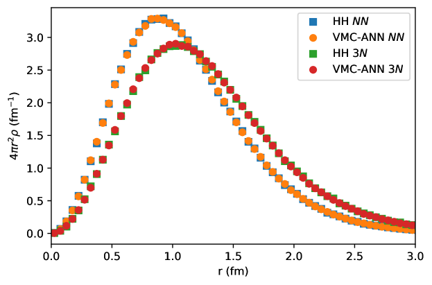
Figure 2: VMC-ANN and HH point-nucleon density of ⁴He as obtained using as input the $NN$ force only or the full $NN$ + $3N$ Hamiltonian.

When the $N\!N$ only is taken as input, VMC-ANN produces ⁶He and ⁶Li wave functions that are stable against breakup into ⁴He plus two neutrons and ⁴He plus deuteron, respectively. This is a highly non-trivial results, as sophisticated VMC calculations of light nuclei that use conventional two- and three-body Jastrow correlations generally fail to get a binding energy for ⁶Li that is below the sum of the one of ⁴He and the deuteron Wiringa:2021p . It remains to be understood whether VMC-ANN would be able to get a stable ⁶Li once more realistic nuclear interactions that include a tensor component are employed. In the $N\!N$ case, the VMC-ANN energies are $\sim 0.5$ MeV less bound than those obtained using the HH approach, corresponding to less than $0.1$ MeV per nucleon. The latter value is not dissimilar from the one we get comparing the VMC-ANN and HH binding energies of ³H and ³He.
The VMC-ANN charge radii are appreciably larger than the HH ones for both ⁶He and ⁶Li nuclei, which are nevertheless smaller than the experimental values. This behavior is reflected in the point-nucleon density of ⁶Li, displayed in Fig. 3. The VMC-ANN distribution extends to larger distances than the HH one. This is partly due the poor quality of the HH in reproducing the long range behaviour of the $A=6$ wave functions, which translates in a very slow convergence rate for the charge radii as function of $K$ — see Ref. Gnech:2020prc for a complete discussion. The relatively small value of $K$ employed in computing $A=6$ nuclei does not allow us to safely extrapolate the computed charge radii, which tend to be underestimated.
Analogous to Fig. 2, the $3N$ interactions broaden the point-nucleon density distributions, depleting their value near $r=0$ and dramatically increasing the charge radius well above its experimental value. In fact, both VMC-ANN and HH calculations with the $3N$ potential yield a ⁶Li that is only barely bound against ⁴He plus deuteron breakup. On the other hand, neither VMC-ANN nor HH calculations that include the $3N$ potential yield a stable ⁶He, as its binding energy is above the one of ⁴He. Hence, its charge radius becomes larger and larger as the wave function keeps extending to larger distances from $\mathbf{R}_{\rm CM}$. This behavior is reminiscent to the one described in Ref. Contessi:2017rww for the ¹⁶O nucleus, which was unbound with respect to breakup into four alpha clusters.

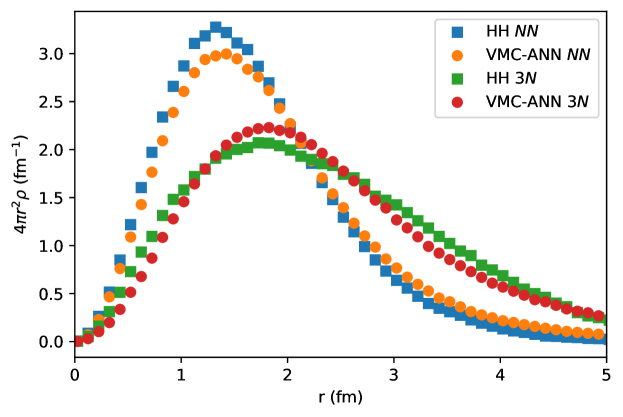
Figure 3: VMC-ANN and HH point-nucleon density of ⁶Li as obtained using as input the $NN$ force only or the full $NN$ + $3N$ Hamiltonian.

5 Conclusion

The development of QMC methods is instrumental for testing predictions and guiding the development of nuclear EFTs, originally proposed by Steven Weinberg. Currently available approaches are either limited to light nuclear systems or to simplified interactions. Novel VMC algorithms based on ANN representation of quantum-mechanical wave functions can potentially overcome these limitations and allow one to make predictions across the nuclear chart using a variety of EFT interactions and currents.

In this work, we extended the reach of the VMC-ANN algorithm introduced in Ref. Adams:2020aax to compute the binding energies and charge radii of $A\leq 6$ nuclei as they emerge from the LO pionless-EFT Hamiltonian of Ref. Schiavilla:2021dun . The VMC-ANN architecture was made more efficient by using as input the pair-wise coordinates of the nucleons instead of the single-particle ones. In addition, treating open-shell $A=6$ nuclei has required summing multiple Slater determinant in the mean-field part of the wave function, which is also expressed in terms of ANNs.

We compare the VMC-ANN binding energies and charge radii of $A\leq 6$ nuclei with the highly accurate HH method. Performing benchmark calculations among different numerical methods corroborates our confidence in the accuracy of the nuclear Schrödinger equation solution Kamada:2001tv ; Maris:2013rgq ; Piarulli:2019pfq . This step is critical to carry out meaningful comparisons of nuclear EFTs’ predictions against experimental data, as it helps to disentangle the uncertainties associated with solving the many-body problem from those pertaining the EFT-based modeling of nuclear dynamics.

There is perfect agreement between the two methods for the simplest ²H nucleus, in terms of both binding energies and charge radii. On the other hand, VMC-ANN underbinds ³H, ³He, and ⁴He nuclei by $\sim 0.2$ MeV with respect to HH. We ascribe the reason for this behavior to deficiencies in the mean-field part of the wave function that cannot be remedied by the ANN correlator. Nevertheless, the charge radii, and point-nucleon densities distributions for these $A\leq 4$ nuclei obtained within the VMC-ANN and HH methods are in excellent agreement, hence demonstrating the flexibility of the ANNs in representing the wave function of light nuclei.

The difference in binding energy per nucleon between the VMC-ANN and HH methods is about $\sim 0.1$ MeV for both ⁶He and ⁶Li; not dissimilar to the one observed for $A\leq 4$ nuclei. The comparison of the VMC-ANN and HH charge radii and the point-nucleon for $A=6$ nuclei presents somewhat bigger discrepancies than in the $A\leq 4$ case. The reason for this behavior is likely twofold. On the one hand, the HH expansion exhibits a slow convergence rate when it comes to reproducing the long-range behavior of the wave function. On the other one, VMC-ANN slightly underbinds these nuclei.

From our analysis, it appears that the ⁶He nucleus is not stable against breakup into ⁴He plus two neutrons at LO in the pionless-EFT expansion, at least for the values of the regulator and LECs that we used. The chief advantage of the Weinberg’s nuclear EFT framework is that it contains the diagnostic tools to assess its convergence. To determine whether ⁶He is bound within pionless-EFT, in addition to using different values of the regulator and LECs, we will employ the next-to-leading (NLO) Hamiltonian of Ref. Schiavilla:2021dun and carry out a rigorous uncertainty quantification on the line of Refs. Furnstahl:2014xsa ; Melendez:2019izc . Concurrently, we will further develop the accuracy of the VMC-ANN method and, thanks to its favorable polonomyal scaling with $A$, we will apply it to larger nuclear systems. The latter point is critical for studying the convergence and the predictive power of both chiral-EFT and pionless-EFT across the nuclear chart.

- (1) S. Weinberg, Phys. Lett. B251, 288 (1990). DOI 10.1016/0370-2693(90)90938-3
- (2) S. Weinberg, Nucl. Phys. B363, 3 (1991). DOI 10.1016/0550-3213(91)90231-L
- (3) S. Weinberg, Phys. Lett. B295, 114 (1992). DOI 10.1016/0370-2693(92)90099-P
- (4) U. van Kolck, Effective Field Theories of Loosely Bound Nuclei (2014), vol. 879, p. 123. DOI 10.1007/978-3-642-45141-6_4
- (5) E. Epelbaum, H.W. Hammer, U.G. Meissner, Rev. Mod. Phys. 81, 1773 (2009). DOI 10.1103/RevModPhys.81.1773
- (6) R. Machleidt, D. Entem, Phys. Rept. 503, 1 (2011). DOI 10.1016/j.physrep.2011.02.001
- (7) P.F. Bedaque, U. van Kolck, Ann. Rev. Nucl. Part. Sci. 52, 339 (2002). DOI 10.1146/annurev.nucl.52.050102.090637
- (8) H. Hergert, Front. in Phys. 8, 379 (2020). DOI 10.3389/fphy.2020.00379
- (9) J. Carlson, S. Gandolfi, F. Pederiva, S.C. Pieper, R. Schiavilla, K. Schmidt, R. Wiringa, Rev. Mod. Phys. 87, 1067 (2015). DOI 10.1103/RevModPhys.87.1067
- (10) K. Schmidt, S. Fantoni, Phys. Lett. B 446, 99 (1999). DOI 10.1016/S0370-2693(98)01522-6
- (11) M. Piarulli, I. Bombaci, D. Logoteta, A. Lovato, R. Wiringa, Phys. Rev. C 101(4), 045801 (2020). DOI 10.1103/PhysRevC.101.045801
- (12) D. Lonardoni, I. Tews, S. Gandolfi, J. Carlson, Phys. Rev. Res. 2, 022033 (2020). DOI 10.1103/PhysRevResearch.2.022033
- (13) S. Gandolfi, D. Lonardoni, A. Lovato, M. Piarulli, Front. Phys. 8, 117 (2020). DOI 10.3389/fphy.2020.00117
- (14) E. Dumitrescu, A. McCaskey, G. Hagen, G. Jansen, T. Morris, T. Papenbrock, R. Pooser, D. Dean, P. Lougovski, Phys. Rev. Lett. 120(21), 210501 (2018). DOI 10.1103/PhysRevLett.120.210501
- (15) A. Roggero, J. Carlson, Phys. Rev. C 100(3), 034610 (2019). DOI 10.1103/PhysRevC.100.034610
- (16) A. Roggero, A. Baroni, Phys. Rev. A 101(2), 022328 (2020). DOI 10.1103/PhysRevA.101.022328
- (17) G. Carleo, I. Cirac, K. Cranmer, L. Daudet, M. Schuld, N. Tishby, L. Vogt-Maranto, L. Zdeborová, Reviews of Modern Physics 91(4), 045002 (2019). DOI 10.1103/RevModPhys.91.045002. URL https://link.aps.org/doi/10.1103/RevModPhys.91.045002
- (18) G. Carleo, M. Troyer, Science 355(6325), 602 (2017). DOI 10.1126/science.aag2302. URL http://science.sciencemag.org/content/355/6325/602
- (19) Y. Nomura, A.S. Darmawan, Y. Yamaji, M. Imada, Physical Review B 96(20), 205152 (2017). DOI 10.1103/PhysRevB.96.205152. URL https://link.aps.org/doi/10.1103/PhysRevB.96.205152
- (20) H. Saito, Journal of the Physical Society of Japan 87(7), 074002 (2018). DOI 10.7566/JPSJ.87.074002. URL https://doi.org/10.7566/JPSJ.87.074002
- (21) K. Choo, G. Carleo, N. Regnault, T. Neupert, Phys. Rev. Lett. 121, 167204 (2018). DOI 10.1103/PhysRevLett.121.167204. URL https://link.aps.org/doi/10.1103/PhysRevLett.121.167204
- (22) Y. Nomura, Journal of the Physical Society of Japan 89(5), 054706 (2020). DOI 10.7566/JPSJ.89.054706. URL https://journals.jps.jp/doi/10.7566/JPSJ.89.054706
- (23) N. Yoshioka, R. Hamazaki, Physical Review B 99(21), 214306 (2019). DOI 10.1103/PhysRevB.99.214306. URL https://link.aps.org/doi/10.1103/PhysRevB.99.214306
- (24) A. Nagy, V. Savona, Physical Review Letters 122(25), 250501 (2019). DOI 10.1103/PhysRevLett.122.250501. URL https://link.aps.org/doi/10.1103/PhysRevLett.122.250501
- (25) F. Vicentini, A. Biella, N. Regnault, C. Ciuti, Physical Review Letters 122(25), 250503 (2019). DOI 10.1103/PhysRevLett.122.250503. URL https://link.aps.org/doi/10.1103/PhysRevLett.122.250503
- (26) M.J. Hartmann, G. Carleo, Physical Review Letters 122(25), 250502 (2019). DOI 10.1103/PhysRevLett.122.250502. URL https://link.aps.org/doi/10.1103/PhysRevLett.122.250502
- (27) F. Ferrari, F. Becca, J. Carrasquilla, Physical Review B 100(12), 125131 (2019). DOI 10.1103/PhysRevB.100.125131. URL https://link.aps.org/doi/10.1103/PhysRevB.100.125131. Publisher: American Physical Society
- (28) D. Pfau, J.S. Spencer, A.e.G.d.G. Matthews, W.M.C. Foulkes, arXiv e-prints arXiv:1909.02487 (2019)
- (29) J. Hermann, Z. Schätzle, F. Noé, arXiv e-prints arXiv:1909.08423 (2019)
- (30) K. Choo, A. Mezzacapo, G. Carleo, Nature Communications 11(1), 2368 (2020). DOI 10.1038/s41467-020-15724-9. URL https://www.nature.com/articles/s41467-020-15724-9
- (31) J.W.T. Keeble, A. Rios, Phys. Lett. B 809, 135743 (2020). DOI 10.1016/j.physletb.2020.135743
- (32) C. Adams, G. Carleo, A. Lovato, N. Rocco, Phys. Rev. Lett. 127(2), 022502 (2021). DOI 10.1103/PhysRevLett.127.022502
- (33) A. Kievsky, S. Rosati, M. Viviani, L. Marcucci, L. Girlanda, J. Phys. G: Nucl. Part. Phys. 35(6), 063101 (2008). DOI 10.1088/0954-3899/35/6/063101
- (34) R. Schiavilla, L. Girlanda, A. Gnech, A. Kievsky, A. Lovato, L.E. Marcucci, M. Piarulli, M. Viviani, Phys. Rev. C 103(5), 054003 (2021). DOI 10.1103/PhysRevC.103.054003
- (35) J.W. Chen, G. Rupak, M.J. Savage, Nucl. Phys. A 653, 386 (1999). DOI 10.1016/S0375-9474(99)00298-5
- (36) R.B. Wiringa, V.G.J. Stoks, R. Schiavilla, Phys. Rev. C 51, 38 (1995). DOI 10.1103/PhysRevC.51.38
- (37) C.J. Yang, Eur. Phys. J. A 56(3), 96 (2020). DOI 10.1140/epja/s10050-020-00104-0
- (38) P.F. Bedaque, H. Hammer, U. van Kolck, Phys. Rev. Lett. 82, 463 (1999). DOI 10.1103/PhysRevLett.82.463
- (39) N. Metropolis, A.W. Rosenbluth, M.N. Rosenbluth, A.H. Teller, E. Teller, J. Chem. Phys. 21, 1087 (1953). DOI 10.1063/1.1699114
- (40) P. Massella, F. Barranco, D. Lonardoni, A. Lovato, F. Pederiva, E. Vigezzi, J. Phys. G 47, 035105 (2020). DOI 10.1088/1361-6471/ab588c
- (41) M. Zaheer, S. Kottur, S. Ravanbakhsh, B. Poczos, R. Salakhutdinov, A. Smola, arXiv e-prints arXiv:1703.06114 (2017)
- (42) E. Wagstaff, F.B. Fuchs, M. Engelcke, I. Posner, M. Osborne, arXiv e-prints arXiv:1901.09006 (2019)
- (43) C. Dugas, Y. Bengio, F. Bélisle, C. Nadeau, R. Garcia, in Advances in Neural Information Processing Systems 13, ed. by T.K. Leen, T.G. Dietterich, V. Tresp (MIT Press, 2001), pp. 472–478. URL http://papers.nips.cc/paper/1920-incorporating-second-order-functional-knowledge-for-better-option-pricing.pdf
- (44) S. Sorella, Phys. Rev. B 71, 241103 (2005). DOI 10.1103/PhysRevB.71.241103. URL http://link.aps.org/doi/10.1103/PhysRevB.71.241103
- (45) L.E. Marcucci, J. Dohet-Eraly, L. Girlanda, A. Gnech, A. Kievsky, M. Viviani, Front. Phys. 8, 69 (2020). DOI 10.3389/fphy.2020.00069. URL https://www.frontiersin.org/article/10.3389/fphy.2020.00069
- (46) A. Gnech, M. Viviani, L.E. Marcucci, Phys. Rev. C 102, 014001 (2020). DOI 10.1103/PhysRevC.102.014001. URL https://link.aps.org/doi/10.1103/PhysRevC.102.014001
- (47) A. Gnech, L.E. Marcucci, R. Schiavilla, M. Viviani, (2021). ArXiv:2016.07439. To be published on Phys. Rev. C
- (48) J. Beringer, et al., Phys. Rev. D 86, 010001 (2012). DOI 10.1103/PhysRevD.86.010001
- (49) J.L. Friar, J. Martorell, D.W.L. Sprung, Phys. Rev. A 56, 4579 (1997). DOI 10.1103/PhysRevA.56.4579
- (50) NNDC (2021), Nudat2, https://www.nndc.bnl.gov/nudat2/
- (51) E. Tiesinga, P.J. Mohr, D.B. Newell, B.N. Taylor, CODATA2018 (2020). Available at http://physics.nist.gov/constants
- (52) A. Amroun, V. Breton, J.M. Cavedon, B. Frois, D. Goutte, F. Juster, P. Leconte, J. Martino, Y. Mizuno, X.H. Phan, S. Platchkov, I. Sick, S. Williamson, Nuclear Physics A 579(3), 596 (1994). DOI https://doi.org/10.1016/0375-9474(94)90925-3. URL https://www.sciencedirect.com/science/article/pii/0375947494909253
- (53) D.C. Morton, Q. Wu, G.W.F. Drake, Phys. Rev. A 73, 034502 (2006). DOI 10.1103/PhysRevA.73.034502. URL https://link.aps.org/doi/10.1103/PhysRevA.73.034502
- (54) J. Krauth, K. Schuhmann, M. Ahmed, et al., Nature 598, 527 (2021). DOI 10.1038/s41586-021-03183-1
- (55) L.B. Wang, P. Mueller, K. Bailey, G.W.F. Drake, J.P. Greene, D. Henderson, R.J. Holt, R.V.F. Janssens, C.L. Jiang, Z.T. Lu, T.P. O’Connor, R.C. Pardo, K.E. Rehm, J.P. Schiffer, X.D. Tang, Phys. Rev. Lett. 93, 142501 (2004). DOI 10.1103/PhysRevLett.93.142501. URL https://link.aps.org/doi/10.1103/PhysRevLett.93.142501
- (56) M. Puchalski, K. Pachucki, Phys. Rev. Lett. 111, 243001 (2013). DOI 10.1103/PhysRevLett.111.243001. URL https://link.aps.org/doi/10.1103/PhysRevLett.111.243001
- (57) R. Wiringa. Private communication
- (58) L. Contessi, A. Lovato, F. Pederiva, A. Roggero, J. Kirscher, U. van Kolck, Phys. Lett. B 772, 839 (2017). DOI 10.1016/j.physletb.2017.07.048
- (59) H. Kamada, et al., Phys. Rev. C 64, 044001 (2001). DOI 10.1103/PhysRevC.64.044001
- (60) P. Maris, J.P. Vary, S. Gandolfi, J. Carlson, S.C. Pieper, Phys. Rev. C 87(5), 054318 (2013). DOI 10.1103/PhysRevC.87.054318
- (61) R.J. Furnstahl, D.R. Phillips, S. Wesolowski, J. Phys. G 42(3), 034028 (2015). DOI 10.1088/0954-3899/42/3/034028
- (62) J.A. Melendez, R.J. Furnstahl, D.R. Phillips, M.T. Pratola, S. Wesolowski, Phys. Rev. C 100(4), 044001 (2019). DOI 10.1103/PhysRevC.100.044001