Deep Adversarially-Enhanced k-Nearest Neighbors

Abstract

Recent works have theoretically and empirically shown that deep neural networks (DNNs) have an inherent vulnerability to small perturbations. Applying the Deep k-Nearest Neighbors (DkNN) classifier, we observe a dramatically increasing robustness-accuracy trade-off as the layer goes deeper. In this work, we propose a Deep Adversarially-Enhanced k-Nearest Neighbors (DAEkNN) method which achieves higher robustness than DkNN and mitigates the robustness-accuracy trade-off in deep layers through two key elements. First, DAEkNN is based on an adversarially trained model. Second, DAEkNN makes predictions by leveraging a weighted combination of benign and adversarial training data. Empirically, we find that DAEkNN improves both the robustness and the robustness-accuracy trade-off on MNIST and CIFAR-10 datasets.

I Introduction

Deep learning has become the backbone of many applications, such as machine translation liu2020multilingual , image classification li2019deep , and object detection wu2020recent . Advanced deep neural network (DNN) models like convolutional neural network (CNN) krizhevsky2012imagenet and recurrent neural network (RNN) graves2013speech result in superiority over conventional models o2019deep . As a side effect, these DNN-based applications only perform well when the input is similar to the examples in the training set, i.e., when the covariate shift of the representation is small compared with the training distribution. A large shift will result in a significant accuracy degradation ben2010theory . More seriously, recent studies have shown that DNNs are easily fooled by adversarial examples, which are well-designed with imperceptible (to the human eyes) perturbations on benign inputs KGB16 ; SZS14 . The lacking of robustness and the big trade-off between the standard performance and the robustness have become bottlenecks of deep learning.

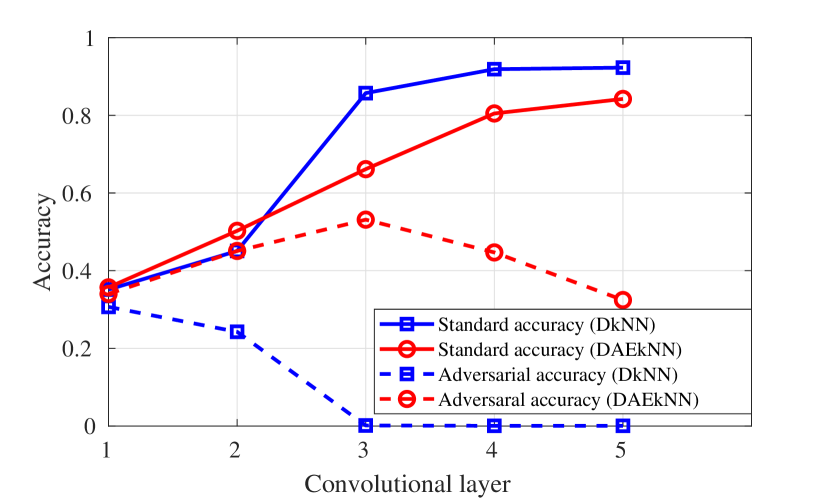
To tackle the problems, various approaches have been proposed. One category of methods is robust training, which mainly focuses on hardening model weights madry17 ; zhang2019theoretically ; cohen2019certified via augmenting benign examples with adversarial perturbations in the training process. This type of method is often tailored to a certain level of attack power, and is restricted to $\ell_{p}$ constraint perturbations. Another category of methods is the adversarial detection metzen2017detecting ; feinman2017detecting ; grosse2017statistical assuming that the adversarial distribution is significantly different from the benign data distribution, which is not always true in practice carlini2017adversarial . Strikingly, k-Nearest Neighbors (kNN)-based deep learning methods are recently demonstrated to have natural robustness defending against adversarial attacks papernot2018deep ; dubey2019defense ; wang2021rails and can be leveraged to tackle other types of data quality issues beyond adversarial examples bahri2020deep . However, the Deep k-Nearest Neighbors (DkNN) method on a standard CIFAR-10 model suffers from poor robustness and big robustness-accuracy trade-off as the layer goes deeper, as illustrated by the blue curves in Figure 1. In this work, we analyze the reasons for the failure of DkNN, and propose a novel robust classifier - Deep Adversarially-Enhanced k-Nearest Neighbors (DAEkNN) that combines the kNN with the adversarial training madry2017towards and a benign-adversarial joint prediction mechanism. We show that DAEkNN can achieve higher robustness and alleviate the robustness-accuracy trade-off compared with DkNN, as illustrated by the red curves in Figure 1.

We make the following contributions in our paper.

• We show that the robustness-accuracy trade-off measured by the Deep k-Nearest Neighbors (DkNN) increases dramatically when the layer goes deeper.

• We propose a Deep Adversarially-Enhanced k-Nearest Neighbors (DAEkNN) method that is based on an adversarially trained madry2017towards model and a benign-adversarial joint prediction mechanism.

• We demonstrate that DAEkNN enhances robustness and alleviates the robustness-accuracy trade-off. Specifically, on MNIST and CIFAR-10 datasets, DAEkNN improves DkNN robustness against PGD attack by $68.2\%$ and $50.42\%$ with $0.88\%$ and $13.34\%$ standard accuracy degradation.

Figure 1: Deep Adversarially-Enhanced k-Nearest Neighbors (DAEkNN) can achieve higher robustness and alleviate the robustness-accuracy trade-off than applying Deep k-Nearest Neighbors (DkNN) on a model trained by standard training. All experiments are conducted on CIFAR-10. Adversarial accuracy is evaluated using $10$-step PGD attack madry2017towards with attack power $\epsilon=8$. The blue curves show the results of DkNN. The red curves show the results of DAEkNN.

II DAEKNN DESIGN

II-A Preliminaries

Throughout this paper, we evaluate different classifiers by measuring three key indices: (i) Standard Accuracy (SA) on benign test examples (ii) Adversarial Accuracy (AA) on the adversarial test examples generated by $10$-step Projected Gradient Descent (PGD) attack madry2017towards and (iii) Harmonic Mean (HM) of AA and SA, which can be calculated by $\frac{2\text{SA}\times\text{AA}}{\text{SA}+\text{AA}}$. HM is determined by both SA and AA, reflecting the robustness-accuracy trade-off to a certain extend.

Projected Gradient Descent (PGD) attack

PGD attack generates adversarial examples $\mathbf{x}_{\delta}=\mathbf{x}+\mathbf{\delta}$ to flip the prediction via maximizing the cross-entropy loss $L$. The generator implements gradient ascent with projection, with the $i$th iterations defined as

$$\mathbf{x}_{\delta}^{i+1}\leftarrow\prod_{\mathcal{C}(\mathbf{x}_{\delta},\epsilon)}\big{[}\mathbf{x}_{\delta}^{i}+\kappa{\rm{sign}}\big{(}\nabla_{\mathbf{x}_{\delta}}L(f_{\theta},\mathbf{x}_{\delta}^{i},y)\big{)}\big{]}$$ (1)

where $f_{\theta}$ is the mapping from DNN input to output. $\kappa$ is the gradient step size. $\prod$ denotes a projection operator, and $\mathcal{C}(\mathbf{x}_{\delta},\epsilon)=\{\mathbf{x}_{\delta}|{\|\mathbf{\delta}\|_{p}}\leq\epsilon,\mathbf{x}_{\delta}\in[v_{\text{lb}},v_{\text{ub}}]^{d}\}$ represents the projection set. Here $\epsilon$ is a positive constant, and we use $\|\cdot\|_{p}=\|\cdot\|_{\infty}$ in this paper. If not otherwise specified, we use the attack power $\epsilon=8/80$ for CIFAR-10/MNIST. $d$ is the input dimension. $[v_{\text{lb}},v_{\text{ub}}]$ is the constraint on the data domain. In this paper, we consider $\mathbf{x}_{\delta}$ as an image vector, thereby $\mathbf{x}_{\delta}\in[0,255]^{d}$.

Deep k-Nearest Neighbors (DkNN)

Different from DNN classifiers, DkNN papernot2018deep combines kNN classifiers that are embedded into selected layers of a DNN, and makes predictions via majority vote among all kNNs. For any test input $\mathbf{x}$, DkNN classifies it to

$$y=\arg\max_{c}\sum_{l\in\mathcal{L}}p_{l}^{c}(\mathbf{x};D_{\text{tr}}^{b}),~{}c\in[C],$$ (2)

where $\mathcal{L}$ is the set of the selected layers and $l\in\mathcal{L}$ is the $l$-th layer of a DNN. $f_{\theta_{l}}$ denotes the mapping from input to layer $l$. Here $p_{l}^{c}(\mathbf{x})$ denotes the confidence score assigned to class $c$ predicted by the corresponding kNN in layer $l$. We use $[C]$ to denote the set $\{1,2,\cdots,C\}$, where $C$ is the number of classes. $D_{\text{tr}}^{b}=(X_{tr}^{b},Y_{tr}^{b})$ is the selected training dataset containing all benign examples $X_{tr}^{b}$ together with their labels $Y_{tr}^{b}$, and $D_{\text{tr}}^{b}(j)=(X_{tr}^{b}(j),Y_{tr}^{b}(j))=(\mathbf{x}_{j},y_{j})$ represents the $j$th example in $D_{\text{tr}}^{b}$. Let $K_{c}^{l}$ be the number of data points belonging to class $c$ among the $K$ nearest neighbors found via measuring $\text{dist}\big{(}f_{\theta_{l}}(\mathbf{x}),f_{\theta_{l}}(X_{tr}^{b}(j))\big{)},\forall j\in|X_{tr}^{b}|$, where $|\cdot|$ means the cardinality of a set. We use $\ell_{2}$ distance for $\text{dist}(\cdot,\cdot)$ by default. The confidence score can be calculated by $p_{l}^{c}(\mathbf{x};D_{\text{tr}}^{b})=\frac{K_{c}^{l}}{K}$.

By default, DkNN is applied on a model trained by standard training. From Figure 1, one can see that the adversarial accuracy obtained by DkNN drops dramatically as the layer goes deeper. As the standard accuracy obtained by DkNN monotonically increases, the robustness-accuracy trade-off also rises. To improve both the robustness and robustness-accuracy trade-off, we introduce a Deep Adversarially-Enhanced k-Nearest Neighbors (DAEkNN) method containing two key components: (i) A DNN model obtained by adversarial training (ii) A joint prediction mechanism leveraging benign and adversarial training data. We introduce each of them in detail below.

Figure 2: The framework of DAEkNN: DAEkNN is based on an adversarially trained deep neural network (DNN) model and a benign-adversarial joint prediction mechanism. In the training phase, a DNN is trained with adversarial data augmentation madry2017towards . In the inference phase, the prediction is made by a joint classifier applied on deep layers of the adversarially trained DNN and combined the k-nearest neighbors (kNN) classifiers based on benign training data and its adversarial counterpart.

II-B Improving Robustness Through Adversarially Trained Model

From Figure 1, one can see that the adversarial accuracy of DkNN drops dramatically as the layer goes deeper, indicating the features learned by DNN lack robustness. In order to robustify k-nearest neighbor classifiers in deep layers, we need the features extracted from those layers to be robust beforehand. Recent works have demonstrated that models trained by standard training tend to learn non-robust features, while models trained by adversarial training madry2017towards are able to extract more robust features engstrom2019adversarial ; wang2021fast ; wang2020practical .

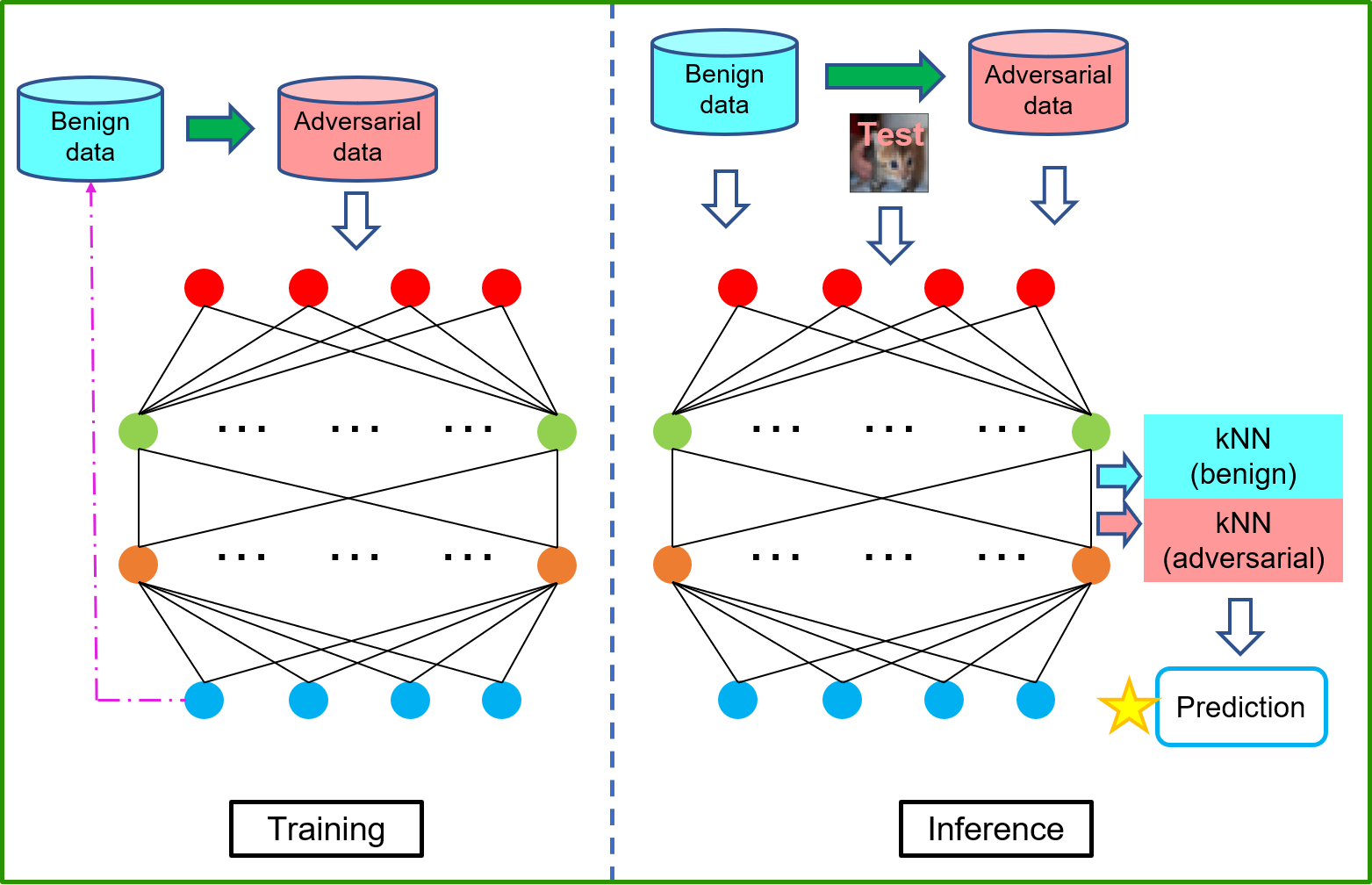
As shown in Figure 2, the adversarial training is performed by updating model weights with adversarial examples generated from benign data in each epoch, and can be characterized by the following optimization problem.

$$\begin{array}[]{ll}\arg\min_{\theta}\frac{1}{|S|}\sum_{(\mathbf{x},y)\in S}\max_{\|\mathbf{\delta}\|_{\infty}\leq\epsilon_{\text{tr}}}L(f_{\theta},\mathbf{x}+\mathbf{\delta},y),\end{array}$$ (4)

where $\epsilon_{\text{tr}}$ is the attack power of the adversarial generator in the training process, and in this paper we fix it to $\epsilon_{\text{tr}}=4$ and $\epsilon_{\text{tr}}=60$ for CIFAR-10 and MNIST, respectively. $S$ denotes a subset of $D_{\text{tr}}^{b}$. We remark that there are different robust training methods madry2017towards ; zhang2019theoretically that can be leveraged to harden DNNs, and we only focus on the adversarial training method madry2017towards .

II-C Improving Robustness Trough Adversarial Training Data

Note that adversarial perturbations are intended to enlarging the gap between the adversarial test distribution and the distribution of the original benign class. Using benign training distribution as the baseline, the covariate shift of the adversarial test distribution is larger than the covariate shift of the benign test distribution. For this reason, when all k-nearest neighbors are found from benign training data, the kNN classifiers are not able to correctly capture the information of the adversarial distribution. Spurred by that, we ask: Is it possible to better handle the covariate shift as well as obtaining more robust classifiers by changing the baseline (benign) distribution to a benign-adversarial combined distribution (in other words, by adding adversarial examples into the kNN searching space)?

Instead of using (2), we propose a benign-adversarial joint prediction mechanism that robustifies classifiers through incorporating the adversarial training data, as illustrated in the inference stage in Figure 2. Mathematically, the benign-adversarial joint prediction is expressed by the following formula.

$$\begin{array}[]{ll}y=\arg\max_{c}\sum_{l\in\mathcal{L}}\big{[}\omega_{a}^{l}p_{l}^{c}(\mathbf{x};D_{\text{tr}}^{a})+\omega_{b}^{l}p_{l}^{c}(\mathbf{x};D_{\text{tr}}^{b})\big{]},c\in[C],\end{array}$$ (6)

where $D_{\text{tr}}^{a}$ denotes the adversarial training data obtained by applying PGD attack on $D_{\text{tr}}^{b}$.

$$\begin{array}[]{ll}D_{\text{tr}}^{a}=\text{PGD}(\theta,\epsilon_{r},D_{\text{tr}}^{b}),\end{array}$$ (8)

Here $D_{\text{tr}}^{a}$ serves as the hardening dataset. We therefore call $\epsilon_{r}$ the hardening strength. We remark that $\epsilon_{r}$ is not as larger as better. For DAEkNN to be useful, we need to ensure that the features extracted by deep layers contain useful class information. For example, a model trained by standard training cannot tolerate large perturbations, and therefore using a large $\epsilon_{r}$ will hurt the performance. In contrast, an adversarially trained model can extract class-relevant features from both benign data and perturbed data. In this sense, an adversarially trained model results in narrower gap between the representations of benign examples and the adversarial examples. $\omega_{a}^{l}$ and $\omega_{b}^{l}$ are weights of the two classifiers. Note that (6) is not a simple mixed up of the benign and adversarial training data. Instead, the new classifier in a single layer is a weighted combination of two classifiers. The weights $\omega_{a}^{l}$, $\omega_{b}^{l}$ are calculated based on the relative distance of the kNN found by the two classifiers.

$$\begin{array}[]{ll}\omega_{a}^{l}=\frac{e^{\text{dist}\big{(}f_{\theta_{l}}(\mathbf{x}),f_{\theta_{l}}(X_{l}^{b})\big{)}}}{e^{\text{dist}\big{(}f_{\theta_{l}}(\mathbf{x}),f_{\theta_{l}}(X_{l}^{b})\big{)}}+e^{\text{dist}\big{(}f_{\theta_{l}}(\mathbf{x}),f_{\theta_{l}}(X_{l}^{a})\big{)}}},\\ \omega_{b}^{l}=\frac{e^{\text{dist}\big{(}f_{\theta_{l}}(\mathbf{x}),f_{\theta_{l}}(X_{l}^{a})\big{)}}}{e^{\text{dist}\big{(}f_{\theta_{l}}(\mathbf{x}),f_{\theta_{l}}(X_{l}^{a})\big{)}}+e^{\text{dist}\big{(}f_{\theta_{l}}(\mathbf{x}),f_{\theta_{l}}(X_{l}^{b})\big{)}}}\end{array}$$ (11)

where $X_{l}^{b}$ denotes the kNN of $\mathbf{x}$ found from $D_{\text{tr}}^{b}$ on layer $l$, and similarly, $X_{l}^{a}$ denotes the kNN of $\mathbf{x}$ found from $D_{\text{tr}}^{a}$ on layer $l$. We use the softmax version of the distance-based weights. One can see that the weight is large when the corresponding distance is small, and $\omega_{a}^{l}+\omega_{b}^{l}=1$.

(6) refines the decision boundaries of (2) by leveraging the combined and weighted classifiers. The implementation details can be viewed in Algorithm 1. We also refer readers to Section III for the ablation study and comparisons.

Algorithm 1 Deep Adversarially-Enhanced k-Nearest Neighbors (DAEkNN)

0  Model $\theta$ trained by adversarial training with $\epsilon_{\text{tr}}$; the selected layers $\mathcal{L}$; hardening strength $\epsilon_{r}$; test input $\mathbf{x}^{\prime}$; number of nearest neighbors $K$.

  Generate $D_{\text{tr}}^{a}$ from $D_{\text{tr}}^{b}$ through (8).

  for All $l\in\mathcal{L}$ do

     Find $K$ nearest neighbors $X_{l}^{b}$ and $X_{l}^{a}$ from $D_{\text{tr}}^{b}$ and $D_{\text{tr}}^{a}$, respectively.

     Count the number of data belonging to class $c$ ($K_{c}^{l}$) among each of $X_{l}^{b}$ and $X_{l}^{a}$.

     Calculate $p_{l}^{c}(\mathbf{x}^{\prime};D_{\text{tr}}^{b})$ and $p_{l}^{c}(\mathbf{x}^{\prime};D_{\text{tr}}^{a})$ using $\frac{K_{c}^{l}}{K}$ obtained from $X_{l}^{b}$ and $X_{l}^{b}$.

     Calculate $\omega_{a}^{l}$, $\omega_{b}^{l}$ through (11).

  end for

  Obtain the final prediction by (6).

  Output: $y$.

III Experimental Results

We compare DAEkNN with standard Convolutional Neural Network (CNN), Adversarially Trained madry2017towards Convolutional Neural Network (AT-CNN), and Deep k-Nearest Neighbors (DkNN) papernot2018deep on MNIST and CIFAR-10 datasets. We implement a three-convolutional-layer architecture for MNIST and the VGG16 architecture for CIFAR-10. VGG16 has five convolutional layer blocks and we call the $i$th block as convolutional layer $i$. By default, we set the attack power $\epsilon_{r}=8/80$ and the hardening strength $\epsilon_{r}=8/60$ for CIFAR-10/MNIST. The performances are measured by Standard Accuracy (SA) evaluated using benign examples, Adversarial Accuracy (AA) evaluated using adversarial examples, and the Harmonic Mean (HM) of SA and AA.

Table I shows the comparisons of different methods. DAEkNN improves DkNN / AT-CNN / CNN robustness against PGD attack by $68.2\%/5.98\%/68.26\%$ and $50.42\%/18.86\%/50.42\%$ with only $0.88\%/0.5\%/1.16\%$ and $13.34\%/7.12\%/13.8\%$ standard accuracy degradation on MNIST and CIFAR-10, respectively. We also compare DAEkNN with DkNN on different layers of VGG16, as shown in Figure 1. One can see that DAEkNN improves DkNN on both the robustness and robustness-accuracy trade-off.

TABLE I: Deep Adversarially-Enhanced k-Nearest Neighbors (DAEkNN) outperforms Convolutional Neural Network (CNN), Adversarially Trained madry2017towards Convolutional Neural Network (AT-CNN), and Deep k-Nearest Neighbors (DkNN) papernot2018deep in terms of Adversarial Accuracy (AA) without appreciable loss of Standard Accuracy (SA) on MNIST and CIFAR-10. Both DAEkNN and DkNN are applied on convolutional layer $2,3$ for MNIST and $3,4$ for CIFAR-10.

		CNN	AT-CNN	DkNN	DAEkNN
MNIST	SA	99.06%	98.4%	98.78%	97.9%
	AA	0%	62.28%	0.06%	68.26%
	HM	0%	76.28%	0.12%	80.44%
CIFAR-10	SA	92.24%	85.56%	91.78%	78.44%
	AA	0.06%	31.62%	0.06%	50.48%
	HM	0.12%	46.18%	0.12%	61.43%

We also consider leave-one-out versions of DAEkNN, which can be viewed as an ablation study. The two variants of DAEkNN are DAEkNN without adversarial training component (DAEkNN-WAT) and DAEkNN without adversarial training data (DAEkNN-WAD). As explained in Section II-C, the hardening strength $\epsilon_{r}$ needs to be set small for a model trained by standard training. We therefore set $\epsilon_{r}=2$ for DAEkNN-WAT. One can see from Table II that even DAEkNN-WAT can significantly improve the robustness of DkNN. With adversarial training data, DAEkNN improves the robustness of DAEkNN-WAD by $3.82\%$.

TABLE II: Comparisons among Deep k-Nearest Neighbors (DkNN) papernot2018deep , Deep Adversarially-Enhanced k-Nearest Neighbors (DAEkNN), DAEkNN without adversarial training component (DAEkNN-WAT), and DAEkNN without adversarial training data (DAEkNN-WAD). Performances are measured by Adversarial Accuracy (AA), Standard Accuracy (SA), and the Harmonic Mean (HM) of AA and SA on CIFAR-10. All methods are applied on convolutional layer $3,4$.

	DkNN	DAEkNN -WAT	DAEkNN -WAD	DAEkNN
SA	91.78%	85.96%	79.9%	78.44%
AA	0.06%	13.1%	46.66%	50.48%
HM	0.12%	22.74%	58.91%	61.43%

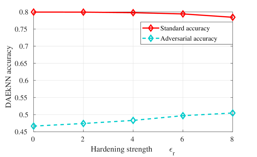
We then study how the hardening strength $\epsilon_{r}$ affects the performance of DAEkNN. As shown in Figure 3, increasing $\epsilon_{r}$ from $0-8$ improves the robustness without appreciable loss of standard accuracy.

Figure 3: Increasing the hardening strength $\epsilon_{r}$ within a certain range ($\leq\epsilon$ in this test) can improve the robustness of Deep Adversarially-Enhanced k-Nearest Neighbors (DAEkNN) without appreciable loss of standard accuracy. All experiments are conducted on CIFAR-10. Adversarial accuracy is evaluated using a $10$-step PGD attack madry2017towards with attack power $\epsilon=8$.

IV CONCLUSION

In this work, we propose a new deep neural network (DNN)-based classifier, called Deep Adversarially-Enhanced k-Nearest Neighbors (DAEkNN), which enjoys high robustness and can mitigate the robustness-accuracy trade-off. We first study the performance of single-layer Deep k-Nearest neighbors (DkNN) on each layer of a DNN. The results indicate that DkNN has poor robustness and big robustness-accuracy trade-offs. The proposed DAEkNN improves robustness through two key adversarial components. DAEkNN extracts features from an adversarially trained model that can provide more robust features. DAEkNN utilizes both the benign training data and adversarial training data in a benign-adversarial joint prediction classifier. The experiments on MNIST and CIFAR-10 demonstrate the effectiveness of DAEkNN.

In future work, we will (i) consider more attack types; (ii) explore the combinations of adversarial training data generated by different hardening strength and different attack types, which could potentially improve the robustness under stronger and unforeseen attacks; (iii) provide a theoretical analysis of the DAEkNN.

References

- [1] Y. Liu, J. Gu, N. Goyal, X. Li, S. Edunov, M. Ghazvininejad, M. Lewis, and L. Zettlemoyer, “Multilingual denoising pre-training for neural machine translation,” Transactions of the Association for Computational Linguistics, vol. 8, pp. 726–742, 2020.
- [2] S. Li, W. Song, L. Fang, Y. Chen, P. Ghamisi, and J. A. Benediktsson, “Deep learning for hyperspectral image classification: An overview,” IEEE Transactions on Geoscience and Remote Sensing, vol. 57, no. 9, pp. 6690–6709, 2019.
- [3] X. Wu, D. Sahoo, and S. C. Hoi, “Recent advances in deep learning for object detection,” Neurocomputing, vol. 396, pp. 39–64, 2020.
- [4] A. Krizhevsky, I. Sutskever, and G. E. Hinton, “Imagenet classification with deep convolutional neural networks,” in Advances in neural information processing systems, 2012, pp. 1097–1105.
- [5] A. Graves, A.-r. Mohamed, and G. Hinton, “Speech recognition with deep recurrent neural networks,” in 2013 IEEE international conference on acoustics, speech and signal processing. Ieee, 2013, pp. 6645–6649.
- [6] N. O’Mahony, S. Campbell, A. Carvalho, S. Harapanahalli, G. V. Hernandez, L. Krpalkova, D. Riordan, and J. Walsh, “Deep learning vs. traditional computer vision,” in Science and Information Conference. Springer, 2019, pp. 128–144.
- [7] S. Ben-David, J. Blitzer, K. Crammer, A. Kulesza, F. Pereira, and J. W. Vaughan, “A theory of learning from different domains,” Machine learning, vol. 79, no. 1, pp. 151–175, 2010.
- [8] A. Kurakin, I. Goodfellow, and S. Bengio, “Adversarial examples in the physical world,” arXiv preprint arXiv:1607.02533, 2016.
- [9] C. Szegedy, W. Zaremba, I. Sutskever, J. Bruna, D. Erhan, I. Goodfellow, and R. Fergus, “Intriguing properties of neural networks,” 2014 ICLR, vol. arXiv preprint arXiv:1312.6199, 2014.
- [10] A. Madry, A. Makelov, L. Schmidt, D. Tsipras, and A. Vladu, “Towards deep learning models resistant to adversarial attacks,” arXiv preprint arXiv:1706.06083, 2017.
- [11] H. Zhang, Y. Yu, J. Jiao, E. P. Xing, L. E. Ghaoui, and M. I. Jordan, “Theoretically principled trade-off between robustness and accuracy,” International Conference on Machine Learning, 2019.
- [12] J. Cohen, E. Rosenfeld, and Z. Kolter, “Certified adversarial robustness via randomized smoothing,” in International Conference on Machine Learning, 2019, pp. 1310–1320.
- [13] J. H. Metzen, T. Genewein, V. Fischer, and B. Bischoff, “On detecting adversarial perturbations,” in International Conference on Learning Representations, 2017.
- [14] R. Feinman, R. R. Curtin, S. Shintre, and A. B. Gardner, “Detecting adversarial samples from artifacts,” arXiv preprint arXiv:1703.00410, 2017.
- [15] K. Grosse, P. Manoharan, N. Papernot, M. Backes, and P. McDaniel, “On the (statistical) detection of adversarial examples,” arXiv preprint arXiv:1702.06280, 2017.
- [16] N. Carlini and D. Wagner, “Adversarial examples are not easily detected: Bypassing ten detection methods,” in Proceedings of the 10th ACM Workshop on Artificial Intelligence and Security. ACM, 2017, pp. 3–14.
- [17] N. Papernot and P. McDaniel, “Deep k-nearest neighbors: Towards confident, interpretable and robust deep learning,” arXiv preprint arXiv:1803.04765, 2018.
- [18] A. Dubey, L. v. d. Maaten, Z. Yalniz, Y. Li, and D. Mahajan, “Defense against adversarial images using web-scale nearest-neighbor search,” in Proceedings of the IEEE/CVF Conference on Computer Vision and Pattern Recognition, 2019, pp. 8767–8776.
- [19] R. Wang, T. Chen, S. Lindsly, C. Stansbury, A. Rehemtulla, I. Rajapakse, and A. Hero, “Rails: A robust adversarial immune-inspired learning system,” arXiv preprint arXiv:2107.02840, 2021.
- [20] D. Bahri, H. Jiang, and M. Gupta, “Deep k-nn for noisy labels,” in International Conference on Machine Learning. PMLR, 2020, pp. 540–550.
- [21] A. Madry, A. Makelov, L. Schmidt, D. Tsipras, and A. Vladu, “Towards deep learning models resistant to adversarial attacks,” arXiv preprint arXiv:1706.06083, 2017.
- [22] L. Engstrom, A. Ilyas, S. Santurkar, D. Tsipras, B. Tran, and A. Madry, “Adversarial robustness as a prior for learned representations,” arXiv preprint arXiv:1906.00945, 2019.
- [23] R. Wang, K. Xu, S. Liu, P.-Y. Chen, T.-W. Weng, C. Gan, and M. Wang, “On fast adversarial robustness adaptation in model-agnostic meta-learning,” 2021.
- [24] R. Wang, G. Zhang, S. Liu, P.-Y. Chen, J. Xiong, and M. Wang, “Practical detection of trojan neural networks: Data-limited and data-free cases,” in Proceedings of the European Conference on Computer Vision (ECCV), 2020.