Dynamics of Ostrowski skew-product: i@. Limit laws and Hausdorff dimensions

Abstract.

We present a dynamical study of Ostrowski’s map based on the use of transfer operators. The Ostrowski dynamical system is obtained as a skew-product of the Gauss map (it has the Gauss map as a base and intervals as fibers) and produces expansions of real numbers with respect to an irrational base given by continued fractions. By studying spectral properties of the associated transfer operators, we show that the absolutely continuous invariant measure of the Ostrowski dynamical system has exponential mixing properties. We deduce a central limit theorem for random variables of an arithmetic nature, and motivated by applications in inhomogeneous Diophantine approximation, we also get Bowen–Ruelle type implicit estimates in terms of spectral elements for the Hausdorff dimension of a bounded digit set.

Dedicated to Jörg Thuswaldner on the occasion of his $50^{th}$ birthday

1. Introduction

We are concerned with the Ostrowski transformation defined on $[0,1)^{2}$ by

$$S(x,y)=\left(\{1/x\},\{y/x\}\right)$$

where $\{.\}$ stands for the fractional part. This is a simple skew-product extension of the Gauss map defined on $[0,1)$ by $x\mapsto\{1/x\}$, which is known to describe dynamically regular continued fraction expansions. The Ostrowski map, introduced in [29], allows the ergodic description of the behaviour of the digits in the associated numeration system (see Proposition 2.1 below).

Various interesting arithmetic, combinatorial or dynamical aspects of the Ostrowski map (and numeration) have been investigated in a wide range of applications from Diophantine approximation to symbolic dynamics. Indeed, classical discrepancy results about Kronecker sequences rely on the use of Ostrowski’s numeration. It is also well-known that the Ostrowski map provides the inhomogeneous best approximations of $y$ in base $x$, as stressed for instance in Ito–Nakada [30], Berthé–Imbert [8] or Beresnevich–Haynes–Velani [6], with the latter providing estimates for sums of reciprocal of fractional parts motivated by applications in multiplicative Diophantine approximation. There is also a deep connection with Sturmian sequences, such as introduced by Morse–Heldund [43], which arise in symbolic dynamics from two-letter codings of orbits under irrational rotations on the unit circle; see e.g., the survey [7] and the references therein. We further refer to Bromberg–Ulcigrai [13] for the use of Ostrowski’s map as a renormalisation tool for temporal limit theorems on deterministic random walks and to Arnoux–Fisher [1] in connection with the geometry of scenery flows of the torus. Lastly, Hara–Ito [26] showed that the Ostrowski numeration yields a characterisation of real quadratic number fields through periodic expansions.

In this article, we discuss dynamical aspects of the Ostrowski map in the context of the study of spectral properties of the associated transfer operators. We observe a Gaussian behavior for Birkhoff sums that gives a refinement of ergodic results from [30], as well as Bowen–Ruelle type estimates for the Hausdorff dimension of fractal sets of pairs of real numbers defined as having bounded digits with respect to Ostrowski’s numeration.

1.1. Homogeneous and inhomogeneous Diophantine approximation

We begin by recalling the general context and some elements of motivation in brief. Denote by $\|\!\cdot\!\|$ the distance to the nearest integer. According to the classical result of Dirichlet, for any irrational number $x$, there exist infinitely many integers $q>0$ such that $q\cdot\|qx\|<1$. Moreover, it is well-known that the best approximations $q$ are given by the convergents of the continued fraction expansion of $x$. This naturally leads to the notion of badly approximable numbers for which there exists $\varepsilon>0$ such that $q\cdot\|qx\|\geq\varepsilon$ for any $q$.

Homogeneous approximation is about the bounds on $\|qx\|$, and it corresponds dynamically to the study of the orbit of $0$ under the action of the irrational rotation on the unit circle ${\mathbb{R}}/{\mathbb{Z}}$. Basically, inhomogeneous Diophantine approximation considers the case of the orbit of any point $y$ by shifting the initial point $0$, i.e., given a point $y$, it deals with the behavior of $\|qx-y\|$.

In the inhomogeneous setting, Minkowski [42] first showed that for any irrational number $x$ and for any real number $y$ which is not of the form $mx+n$, with $m$ and $n$ being integers, then

$$\liminf_{|q|\rightarrow\infty}|q|\!\cdot\!\|qx-y\|\leq\frac{1}{4}.$$

Note that this bound has been improved by Khintchine [35] in the setting of one-sided approximation (i.e., when we consider positive integers $q$) to $1/\sqrt{5}$, for any real number $y$. See also [17, 19, 21, 46] for related results on the sequence of inhomogeneous minima based on the use of Ostrowski’s numeration.

Thus, it is natural to consider the inhomogeneous analogue of the notion of badly approximable numbers: for an irrational number $x$ and for $\varepsilon>0$, set

(1.1) $$B(x,\varepsilon)=\left\{y\in{\mathbb{R}}:\liminf_{|q|\rightarrow\infty}|q|\!\cdot\!\|qx-y\|\geq\varepsilon\right\}.$$

When $q$ is assumed to be positive, it is also simply possible to consider one-sided approximations; see for instance [36, 19, 15].

Some questions arising from Diophantine approximations, either in the homogeneous or in the inhomogeneous case, are typically related to the Hausdorff dimension estimate of the set of badly approximable numbers, with techniques from metric number theory or homogeneous dynamics. Recall indeed that $x$ is badly approximable if and only if the partial quotients of its continued fraction expansion are bounded. Thus the study of bounded type fractal sets arises in a natural way: for a given integer $N\geq 2$, denote by $C_{N}$ the set of real numbers $x\in[0,1)$ which admit a continued fraction expansion $x=[0;a_{1},a_{2},\ldots]$ with all $a_{i}$ satisfying $1\leq a_{i}\leq N$. A powerful approach towards the study of the Hausdorff dimension of $C_{N}$ is provided by the thermodynamic formalism via transfer operators and dynamical determinants, leading to a Bowen–Ruelle type spectral characterisation for the Hausdorff dimension of $C_{N}$. We refer to Hensley [28, 27], Cesaratto–Vallée [18] and Jenkinson–Gonzalez–Urbański [32]. We also refer to Jenkinson–Pollicott [33] for an explicit numerical computation on the Hausdorff dimension of $C_{N}$ in the context of Zaremba’s conjecture and to Das–Fishman–Simmons–Urbański [20] for strengthening Hensley’s formula via small perturbations of a conformal iterated function system.

The situation for inhomogeneous approximation is more contrasted; see for instance [36, 14, 40]. In contrast with the homogeneous case, it is proved in particular by Bugeaud–Kim–Lim–Rams [15] that the set $B(x,\varepsilon)$ (defined in (1.1)) has full Hausdorff dimension for some positive $\varepsilon$ if and only if $x$ is singular on average, which is equivalent to the average of the logarithms of the partial quotients to tend to infinity. See also recent works of Kim–Liao [37] for uniform inhomogeneous approximation or Bugeaud–Zhang [16] for the field of formal power series.

In the meanwhile, there has been no development of a spectral approach in the inhomogeneous setting. We set up the first steps in this direction. Here, we introduce and study a concrete dynamical formulation for a certain bounded-type set (see (1.3) below), motivated by inhomogeneous Diophantine approximation that arises from the Ostrowski expansion (see also the discussion at the end of §5). One reason for this specific choice of digits is that it allows an explicit geometric description of fundamental digit sets (i.e., sets of real numbers having the same given number of first pairs of digits $(a,b)$ when applying the Ostrowski map, such as described in §2.2) in terms of quadrangulars that will provide suitable covers for the Hausdorff estimates (see Figure 3).

1.2. Set up and main results

The Ostrowski transformation $S$ is defined on $[0,1)^{2}$ by $S(x,y)=\left(\{1/x\},\{y/x\}\right)$. Let $(x,y)=(x_{0},y_{0})$ and $(x_{i},y_{i})=S^{i}(x,y)$ for all $i\geq 1$. We then get two sequences $(a_{i})_{i}$ and $(b_{i})_{i}$ of non-negative integers given by $a_{i}=\lfloor\frac{1}{x_{i-1}}\rfloor$ and $b_{i}=\lfloor\frac{y_{i-1}}{x_{i-1}}\rfloor$ ($i\geq 1$). Note that the sequence $(a_{i})_{i}$ provides the continued fraction expansion of $x=[0;a_{1},a_{2},\ldots]$. We denote by $\frac{p_{i}}{q_{i}}=[0;a_{1},\ldots,a_{i}]$ the $i$-th convergent of $x$ and set $\theta_{i}:=q_{i}x-p_{i}$. Then the sequence $(b_{i})_{i}$ yields the expansion $y=\sum_{i=1}^{\infty}b_{i}|\theta_{i-1}|$ for $y$ with respect to $x$. Moreover, the sequence of digits $(b_{i})_{i}$ satisfies the admissibility conditions stated in next proposition which guarantee uniqueness of such an expansion. We refer to Proposition 2.1 and §7 for more precise details. See also Barat–Liardet [5] or Berthé [7] for further reading on the Ostrowski numeration system. In particular, a related numeration system is defined for integers as a generalisation of the Zeckendorf representation which involves Fibonacci numbers and the golden ratio.

Proposition 1.1 (Ostrowski numeration system).

Let $x\in[0,1)\backslash{\mathbb{Q}}$. Let $(a_{i})$ stand for the sequence of partial quotients in the continued fraction expansion of $x$. Every real number $y\in[0,1)$ can be written uniquely in the form

$$y=\sum_{i=1}^{\infty}b_{i}|\theta_{i-1}|$$

where $0\leq b_{i}\leq a_{i}$ for all $i\geq 1$, if $a_{i}=b_{i}$ for some $i$, then $b_{i+1}=0$, and $a_{i}\neq b_{i}$ for infinitely many odd and even indices $i$.

In view of Proposition 1.1, Ostrowski’s numeration can be defined with respect either to the basis $(|\theta_{i}|)_{i}$ or to the basis $(\theta_{i})_{i}$. Accordingly, there are various dynamical systems associated with Ostrowski’s numerations such as discussed e.g. in [29, 30], which share a strong resemblance. We have chosen to focus here on the simplest one which has moreover the particularity of being formally close at first sight to the two-dimensional continued fraction algorithm Jacobi–Perron algorithm, which is among the most famous continued fraction algorithm (see Remark 2.2 for more details on this comparison).

Proposition 1.1 enables us to see that the Ostrowski transformation provides inhomogeneous approximations of $y=\sum_{i=1}^{\infty}b_{i}|\theta_{i-1}|=\sum_{i=1}^{\infty}b_{i}(-1)^{i-1}\theta_{i-1}$ in base $x$. More precisely, setting

(1.2) $$M_{n}:=\sum_{i=1}^{n}b_{i}(-1)^{i-1}q_{i-1},$$

the sequence $(M_{n})_{n\geq 1}$ yields a sequence of approximants such that $M_{n}x$ converges to $y$ modulo $1$. See §2.1 for more details and also §5.

Motivated by the study of badly approximable numbers, we consider the following bounded-type set of points whose Ostrowski expansion admits restricted digits. Fix an integer $N\geq 2$, and set

(1.3) $$E_{N}=\{(x,y)\in[0,1)^{2}:1\leq a_{i}\leq N\ \mbox{and }b_{i}=a_{i}-1,\ \mbox{for all }i\geq 1\}.$$

We study the Hausdorff dimension of $E_{N}$. We further ask how often the digit condition of (1.3) happens. For instance, consider for all $n\geq 1$ and $x=[0;a_{1},a_{2},\ldots,a_{n},\ldots]$

(1.4) $$D_{N,n}(x,y)=\#\{1\leq i\leq n:a_{i}\leq N\ \mbox{and }b_{i}=a_{i}-1\}.$$

Regarding $D_{N,n}$ as a random variable over pairs of real numbers in $[0,1)^{2}$, we study its limiting behavior as $N$ goes to infinity. Notice that

$$D_{N,n}(x,y)=\sum_{i=1}^{n}f(a_{i},b_{i})=\sum_{i=1}^{n}f\left(\left\lfloor\frac{1}{x_{i-1}}\right\rfloor,\left\lfloor\frac{y_{i-1}}{x_{i-1}}\right\rfloor\right)$$

where $f$ is the membership function given by $f(a,b)={\mathbf{1}}_{\leq N}(a){\mathbf{1}}_{a-1}(b)$. Simply the quantity $D_{N,n}$ can be understood as a Birkhoff sum of the Ostrowski map.

Now we describe our approach, which is both dynamical and functional, being based on classical transfer operator techniques. For complex parameters $s,w$ and for some observable $f:I^{2}\rightarrow{\mathbb{R}}^{+}$, consider the weighted transfer operator associated to the Ostrowski map

(1.5) $${\mathcal{L}}_{s,w}\phi(x,y)=\sum_{(a,b)\atop 0\leq b\leq a,1\leq a}\frac{\exp\left(w\!\cdot\!f\left(\frac{1}{a+x},\frac{b+y}{a+x}\right)\right)}{(a+x)^{3s}}\phi\left(\frac{1}{a+x},\frac{b+y}{a+x}\right)\cdot{\mathbf{1}}_{SI_{a,b}}(x,y)$$

whenever the series converges (see §2.4 for a precise assumption), where $I_{a,b}$ denotes stands for the interior of the set of points $(x,y)$ satisfying $\lfloor 1/x\rfloor=a$ and $\lfloor y/x\rfloor=b$. In this article, we study spectral properties of the operator for $(s,w)$ close to $(1,0)$, and for a given function $f:I^{2}\rightarrow{\mathbb{R}}^{+}$ assumed to be of moderate growth, i.e., $f\circ{\mathbf{h}}_{a,b}=O(\log a)$ for all $(a,b)\in{\mathcal{A}}$; we use the fact that the parameters $s$ and $w$ are related to the study of probabilistic limit theorems for Birkhoff sums and to Hausdorff dimensions, respectively.

In order to study the spectrum of this operator, the main difficulty is to deal with the characteristic functions ${\mathbf{1}}_{SI_{a,b}}$ that appear in (1.5), which precisely comes from the digit conditions from Proposition 1.1. However, for the Ostrowski map, the usual and well-known function spaces, e.g. $C^{1}$ (used in [4] for the study of Gauss map), or else the set of Hölder functions, are not invariant under the action of the transfer operator. We have chosen to adapt the strategy of Mayer [41] developed for a class of locally expanding maps of $[0,1]^{d}$, to the current Ostrowski setting. The operator is then proved to be compact which we plan to use for further numerical estimates (as e.g. in [33]). We also follow Broise [11] which handles the case of the Jacobi–Perron algorithm; this allows us to strengthen the comparison between both algorithms. The associated dynamical system is not a skew product but a two-dimensional continued fraction algorithm, however it shares common features with the Ostrowski’s map (see Remark 2.2 for more details).

We thus observe the existence of a coarse topological partition for $[0,1)^{2}$ with the two following disjoint subsets $\Delta_{0}=\{(x,y):y<x\}$ and $\Delta_{1}=\{(x,y):x<y\}$. This allows us to interpret the behavior of the transfer operator with respect to the multiplication by characteristic functions in terms of the admissibility between two partitions $I_{a,b}$ and $\Delta_{i}$ (see §3.1 for precise details). From this, we introduce a generalised transfer operator. For each $i\in\{0,1\}$, define

(1.6) $${\widetilde{\mathcal{L}}}_{i,(s,w)}\Phi(x,y)=\sum_{j\in\{0,1\}}\sum_{(a,b)\in{\mathcal{A}}_{i,j}}\frac{\exp\left(w\!\cdot\!f\left(\frac{1}{a+x},\frac{b+y}{a+x}\right)\right)}{(a+x)^{3s}}\cdot\Phi_{j}\left(\frac{1}{a+x},\frac{b+y}{a+x}\right)$$

where $\Phi=(\Phi_{0},\Phi_{1})$ with $\Phi_{i}$ acting on $\Delta_{i}$, and ${\mathcal{A}}_{i,j}$ is the set of pairs of digits $(a,b)$ (with $a\geq 1$, $0\leq b\leq a$) such that for each $i$, the associated inverse branch ${\mathbf{h}}_{a,b}$ maps $\Delta_{i}$ to $\Delta_{j}$.

The generalised transfer operator is almost similar to ${\mathcal{L}}_{s,w}$ but it will act on the function space with an additional index $i$ for the modified partition $\{\Delta_{i}\}_{i\in\{0,1\}}$. More precisely, we consider locally holomorphic functions described in terms of the space of “pairs” of functions that are holomorphic on $\Omega\subseteq{\mathbb{C}}^{2}$, where $\Omega$ is a bounded domain on which the inverse branches of the Ostrowski map can be analytically continued, defined as follows:

$${\widetilde{{\mathcal{B}}}}(\Omega)=\{\Phi=(\Phi_{0},\Phi_{1}):\Omega\rightarrow{\mathbb{C}}:\Phi_{i}\ \mbox{is bounded and holomorphic for }i=0,1\}.$$

This is a Banach space when endowed with the norm

$$\|\Phi\|=\sup_{i\in\{0,1\}}\sup_{(u,v)\in\Omega}|\Phi_{i}(u,v)|$$

on which the generalised transfer operator ${\widetilde{\mathcal{L}}}_{s,w}=({\widetilde{\mathcal{L}}}_{0,(s,w)},{\widetilde{\mathcal{L}}}_{1,(s,w)})$ acts properly when $(s,w)$ is close to $(1,0)$ and $f$ is assumed to be of moderate growth, i.e., $f\circ{\mathbf{h}}_{a,b}=O(\log a)$ for all $(a,b)$ satisfying $1\leq a$, $0\leq b\leq a$. Then we first observe the following.

Theorem A (Theorem 4.7).

The operator ${\widetilde{\mathcal{L}}}_{s,w}$ on ${\widetilde{{\mathcal{B}}}}(\Omega)$ is compact. In particular, it has a simple largest eigenvalue $\lambda_{s,w}$ whose modulus is strictly larger than all other eigenvalues.

A relation between ${\widetilde{\mathcal{L}}}_{s,w}$ and ${\mathcal{L}}_{s,w}$ can be clearly seen. Set $(\kappa\Phi)(x,y):=\Phi_{i}(x,y)$ if $(x,y)\in\Delta_{i}$, then we get $\kappa({\widetilde{\mathcal{L}}}_{s,w}\Phi)={\mathcal{L}}_{s,w}(\kappa\Phi)$. This specialisation shows that ${\mathcal{L}}_{s,w}$ has an eigenfunction $\kappa\Phi_{s,w}$ in the space $L^{1}([0,1]^{2})$ with the same eigenvalue $\lambda_{s,w}$. Together with the density of periodic points in Proposition 2.9, the spectral gap from Theorem A allows us to see that there exists an absolutely continuous invariant measure $\mu$ for the Ostrowski map, whose density is locally holomorphic (its explicit expression, due to Ito [29], is given in Remark 4.5). This further leads to:

Theorem B (Proposition 4.4 and Theorem 5.1).

The Ostrowski dynamical system has exponential mixing with respect to $\mu$. Therefore, we have a central limit theorem for Birkhoff sums. For given $f$ under mild assumptions and for $z\in{\mathbb{R}}$

$$\mu\left\{\frac{1}{\sqrt{n}}S_{n}f\leq z\right\}\longrightarrow\frac{1}{\sigma\sqrt{2\pi}}\int_{-\infty}^{z}e^{-t^{2}/2\sigma^{2}}dt$$

for a suitable constant $\sigma$ as $n$ goes to infinity.

Remark that this comes from the argument that the moment generating function of a Birkhoff sum $S_{n}f$ can be written in terms of transfer operators ${\widetilde{\mathcal{L}}}_{1,\frac{it}{\sqrt{n}}}^{n}$ (following now the classical approach initiated by Nagaev, see e.g. Broise [12]). Thus specialising $f$, we observe a Gaussian behavior for various Diophantine parameters.

Finally, we consider the operator ${\mathcal{L}}_{N,s}:={\mathcal{L}}_{N,s,0}$, whose summand is constrained with digits $(a,b)$ satisfying the condition in (1.3). Notice that the operator ${\mathcal{L}}_{N,s}$ satisfies Theorem A with the largest eigenvalue $\lambda_{N,s}$. Together with explicit estimates on the diameter of the partition $I_{a,b}$ (see Proposition 2.7) and a bounded distortion property of the Jacobian determinant (see Proposition 6.1), we have the following spectral description for the Hausdorff dimension of $E_{N}$.

Theorem C (Proposition 6.2 and 6.3).

Consider the restriction $S|_{E_{N}}$ and its associated transfer operator ${\mathcal{L}}_{N,s}$. Then we have

$$3s_{1}/2\leq\dim_{H}(E_{N})\leq\min\{s_{2},3s_{1}\}$$

for real variables $s_{1},s_{2}$ satisfying $\lambda_{N,s_{1}}=1$ and $(N+1)^{2s_{2}}\lambda_{N,s_{2}}=1$.

When the upper and lower bound is the same, this type of implicit characterisation is usually called a Bowen–Ruelle formula. Bowen [10] first showed that the Hausdorff dimension of a conformal repeller for quasicircles is equal to the zero of a pressure function. This study was further developed by Ruelle [44] for more general hyperbolic settings in terms of transfer operators. For the continued fraction case, there have been analogous results in the setting of homogeneous Diophantine approximation (see e.g. [18, 27, 28, 32]).

We remark that Theorem C is among the first such examples in inhomogeneous approximation and also for maps related to multidimensional continued fractions; note that estimates for the Hausdorff dimension of the Rauzy gasket and for the Arnoux–Rauzy continued fractions have been established in [2, 23, 25]. However, the present approach (i.e., the choice of coverings by the quadrangulars from Proposition 2.7) is not sufficient for obtaining a more precise spectral description in higher dimension with non-conformality. Note that the upper bound in Theorem C is not expected to be optimal; also the quantity $s_{1}$ from Theorem C is related to an analogous quantity for the Gauss map. We plan to refine such estimates in a subsequent paper.

We outline the contents of this paper as follows. In §2, we discuss basic dynamical properties of the Ostrowski map and of its transfer operator. In §3, we introduce a finite modified Markov partition and its associated generalised transfer operator. In §4, we study the spectral properties of these generalised transfer operators acting on a suitable Banach space. This leads us to have a central limit theorem in §5 and elements of description for the Hausdorff dimension of a fractal set of bounded digit type arising from the Ostrowski expansion in §6. In §7, we give a supplementary exposition to some arithmetic identities as well as arithmetical proofs.

Acknowledgements

We would like to thank François Ledrappier for his careful reading and for significantly improving the first draft. We thank Eda Cesarrato and Lingmin Liao for suggesting the refinements in Proposition 6.2 and Proposition 6.3, and also Viviane Baladi, Charles Fougeron, Brigitte Vallée and Benedict Sewell for stimulating discussions and clarifying comments. Finally, we owe much to the referee for his/her perceptive suggestions.

2. The Ostrowski dynamical system

2.1. Arithmetical identities

Let $I^{2}=[0,1)^{2}$. The Ostrowski map $S:I^{2}\rightarrow I^{2}$ is given by

$$S(x,y)=\left(\{1/x\},\{y/x\}\right)\mbox{ for }x\neq 0,\quad S(0,y)=\left(0,0\right).$$

This is a skew-product extension of the Gauss map, which is defined on the unit interval $I=[0,1)$ by $T:x\mapsto\{1/x\}$. For $(x,y)\in I^{2}$, set $(x_{0},y_{0}):=(x,y)$ and $(x_{i},y_{i}):=S^{i}(x,y)$ for all $i\geq 1$. Then the sequence of (pairs of) digits produced by the Ostrowski map is defined as follows, for all positive integer $i$:

$$(a_{i},b_{i})=\left(\left\lfloor\frac{1}{x_{i-1}}\right\rfloor,\left\lfloor\frac{y_{i-1}}{x_{i-1}}\right\rfloor\right)\mbox{ if }x_{i-1}\neq 0,\mbox{ otherwise }(a_{i},b_{i})=0.$$

We also recall that $(a_{i})_{i}$ provides the sequence of partial quotients in the continued fraction expansion of $x=[0;a_{1},a_{2},\cdots]$, $\frac{p_{i}}{q_{i}}=[0;a_{1},\cdots,a_{i}]$ stands for the $i$-th convergent of $x$, and $\theta_{i}:=q_{i}x-p_{i}$ for all $i\geq 1$.

We first state some classical identities concerning regular continued fractions. Let $x\in[0,1)$. Then, for $n\geq 0$, one has

(2.1) $$x=\frac{p_{n}+T^{n}(x)p_{n-1}}{q_{n}+T^{n}(x)q_{n-1}}$$

and

(2.2) $$xT(x)\cdots T^{n-1}(x)=\frac{1}{q_{n}+T^{n}(x)q_{n-1}}=|q_{n-1}x-p_{n-1}|=|\theta_{n-1}|.$$

Note that (2.1) and (2.2) can easily be deduced from the classical matricial representation of continued fractions. Indeed, one has

$$\left[\begin{array}[]{l}x\\ 1\end{array}\right] =xT(x)\cdots T^{n-1}(x)\left[\begin{array}[]{ll}0&1\\ 1&a_{1}\end{array}\right]\cdots\left[\begin{array}[]{ll}0&1\\ 1&a_{n}\end{array}\right]\begin{bmatrix}T^{n}(x)\\ 1\end{bmatrix}$$

$$=xT(x)\cdots T^{n-1}(x)\left[\begin{array}[]{ll}p_{n-1}&p_{n}\\ q_{n-1}&q_{n}\end{array}\right]\begin{bmatrix}T^{n}(x)\\ 1\end{bmatrix}.$$

For the action of the Ostrowski map $S$ on the skew coordinate, note that we have $y_{i-1}=x_{i-1}(y_{i}+b_{i})$ ($i\geq 1$), and thus this yields for all positive $n$ that

$$y=x_{0}x_{1}\cdots x_{n-1}y_{n}+\sum_{i=1}^{n}x_{0}x_{1}\cdots x_{i-1}b_{i}.$$

Note that the series $\sum_{i\geq 1}^{\infty}b_{i}|\theta_{i-1}|$ is convergent (with $0\leq b_{i}\leq a_{i}$ for all $i$). Indeed, for all positive $i$, one has $b_{i}|\theta_{i-1}|=b_{i}|q_{i-1}x-p_{i-1}|\leq\frac{a_{i}}{q_{i}}\leq\frac{1}{q_{i-1}}$; we conclude by observing that $q_{i}\geq(\frac{1+\sqrt{5}}{2})^{i}$ for all $i$.

Together with the identity $x_{0}x_{1}\cdots x_{i}=(-1)^{i}\theta_{i}=|\theta_{i}|$ ($i\geq 0$), we deduce that the sequence of digits $(b_{i})_{i}$ provides the expansion of $y$ in terms of the Ostrowski numeration system from Proposition 1.1.

Observe moreover by (2.2) that

$$0\leq y-\sum_{i=1}^{n}b_{i}|\theta_{i-1}|=y_{n}x_{0}\cdots x_{n-1}=y_{n}|\theta_{n-1}|=\frac{y_{n}}{q_{n}+q_{n-1}x_{n}}<1/q_{n}$$

since $0\leq x_{n},y_{n}\leq 1$. Hence, by recalling that $\|\!\cdot\!\|$ stands for the distance to the nearest integer, one has $\|y-\sum_{i=1}^{n}b_{i}|\theta_{i-1}|\|=y-\sum_{i=1}^{n}b_{i}|\theta_{i-1}|.$ Since $\sum_{i=1}^{n}b_{i}|\theta_{i-1}|=\sum_{i=1}^{n}b_{i}(-1)^{i}\theta_{i-1}$ is congruent modulo 1 to $(\sum_{i=1}^{n}b_{i}(-1)^{i-1}q_{i})x$, one gets

$$\|y-(\sum_{i=1}^{n}b_{i}(-1)^{i-1}q_{i})x\|=y-\sum_{i=1}^{n}b_{i}|\theta_{i-1}|=\sum_{i\geq n+1}^{n}b_{i}|\theta_{i-1}|.$$

Hence, the sequence $(M_{n})_{n}$, with $M_{n}=\sum_{i=1}^{n}b_{i}q_{i-1}(-1)^{i-1}$ (such as defined in (1.2)), is such that $\|y-M_{n}x\|=\sum_{i=n+1}^{\infty}b_{i}|\theta_{i-1}|$. Moreover, one has $|\theta_{i}|=|\theta_{i-2}|-a_{i}|\theta_{i-1}|$ for all $i\geq 1$. One then deduces by using telescoping sums that for $n\geq 1$

(2.3) $$\sum_{i=n}^{\infty}a_{i}|\theta_{i-1}|=|\theta_{n-2}|+|\theta_{n-1}|$$

and thus $\sum_{i=n+1}^{\infty}b_{i}|\theta_{i-1}|\leq|\theta_{n-1}|+|\theta_{n}|,$ which implies that the sequence $(M_{n}x)_{n}$ tends to $y$ modulo $1$ at exponential speed.

We now state a more complete version of Proposition 1.1, whose proof is given below in §7.

Proposition 2.1 (Ostrowski expansions).

Let $x\in[0,1)\backslash{\mathbb{Q}}$. Every real number $y\in[0,1)$ can be written in the form

(2.4) $$y=\sum_{i=1}^{\infty}b_{i}|\theta_{i-1}|$$

where the sequence $(b_{i})_{i}$ is given by the Ostrowski map $S$ applied to $(x,y)$.

Moreover, for any $(x,y)\in[0,1)^{2}$, the sequence $(a_{i},b_{i})_{i}$ of digits coming from the trajectories of the Ostrowski map $S$ satisfies the following admissibility properties:

1. $0\leq b_{i}\leq a_{i}$ for all $i\geq 1$;

2. if $a_{i}=b_{i}$ for some $i$, then $b_{i+1}=0$;     (Markov condition)

3. $a_{i}\neq b_{i}$ for infinitely many odd and even indices $i$.

Moreover, an expansion of the form (2.4) is unique provided that the sequence of digits $(b_{i})$ satisfies these admissibility conditions.

Remark 2.2.

The Ostrowski map is quite similar to the 2-dimensional Jacobi–Perron continued fraction algorithm. The Jacobi–Perron map is defined on $I^{2}$ by $\operatorname{T_{JP}}:(x,y)\mapsto\left(\{y/x\},\{1/x\}\right)$ if $x\neq 0$, and $(0,y)\mapsto(0,0).$ It produces a multi-dimensional continued fraction algorithm whereas the Ostrowski map is a skew-product of the Gauss map. The digits produced by the Jacobi–Perron algorithm satisfy a similar Markovian condition. Indeed, if $(a_{n},b_{n})=\left(\left\lfloor\frac{1}{x_{n-1}}\right\rfloor,\left\lfloor\frac{y_{n-1}}{x_{n-1}}\right\rfloor\right)$ with $(x_{n},y_{n})=\operatorname{T_{JP}}^{n}(x,y)$ for all $n\geq 1$, then one has for all $n\geq 1$, $0\leq b_{n}\leq a_{n}$, $a_{n}\geq 1$ and if $a_{n}=b_{n}$ then $b_{n+1}\geq 1$.

For more on its dynamical study and its exponential convergence properties, see e.g., Lagarias [39] and Broise [11].

2.2. On Ostrowski’s partition

In this section, we study the Ostrowski map from a dynamical point of view. We introduce the fundamental digit partition and discuss some basic properties.

Let us first decompose $I^{2}=[0,1)^{2}$ into the following countable partition given by the “cylinders”, i.e., the sets of real numbers in $I^{2}$ having the same first pair of digits $(a,b)$ when applying the Ostrowski map $S$. More precisely, for any $x\in(0,1)$, there exists a unique positive integer $a$ such that $a\leq\frac{1}{x}<a+1$ (i.e., $a=\lfloor 1/x\rfloor$). This means that it gives the first digit of the continued fraction expansion of $x$, i.e., $x=[0;a,\cdots]$. Then for any $y\in[0,1)$, there exists a unique integer $b$ (i.e., $b=\lfloor y/x\rfloor\geq 0$) such that $bx\leq y<(b+1)x$. Here, we always have $b\leq a$ since $y<1$. Thus for any integers $a,b$ satisfying $a\geq 1$ and $0\leq b\leq a$, set

$$I_{a,b}:=\left\{(x,y)\in I^{2}:\frac{1}{a+1}<x<\frac{1}{a},\ bx<y<(b+1)x\right\}.$$

The set $I_{a,b}$ is the interior of the set of points $(x,y)\in I^{2}$ satisfying $\lfloor 1/x\rfloor=a,$ $\lfloor y/x\rfloor=b.$ Let us denote by ${\mathcal{A}}$ the set of digits $(a,b)$, i.e.,

$${\mathcal{A}}=\{(a,b)\in{\mathbb{Z}}^{2}:1\leq a,\ 0\leq b\leq a\}.$$

Then it follows that $\{I_{a,b}\}_{(a,b)\in{\mathcal{A}}}$ forms a countable topological partition for $I^{2}$, called the fundamental digit partition. The atoms of this partition are called fundamental digit sets. They are either triangles or quadrangulars. See Figure 1 for an illustration.

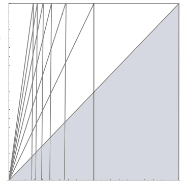
Figure 1. Partition $I_{a,b}$ for $(a,b)\in{\mathcal{A}}$. The set $\Delta_{0}$ is depicted in light grey.

The restriction of the map $S$ on each partition element $I_{a,b}$ is one-to-one, hence it is a bijection onto its image $S(I_{a,b})$ (given in Lemma 2.3 below). For any $(a,b)\in{\mathcal{A}}$, let ${\mathbf{h}}_{a,b}$ stand for the inverse branch of the restriction of $S$ to $I_{a,b}$. Note that it has a simple homographic form:

(2.5) $${\mathbf{h}}_{a,b}(x,y)=\left(\frac{1}{a+x},\frac{b+y}{a+x}\right).$$

To describe the image $S(I_{a,b})$, we divide the index set ${\mathcal{A}}$ into two disjoint subsets. Set

$${\mathcal{A}}_{0}:=\{(a,b)\in{\mathcal{A}}:a=b\}\mbox{ and }{\mathcal{A}}_{1}:=\{(a,b)\in{\mathcal{A}}:0\leq b<a\}.$$

We may also divide $I^{2}$ into two pieces, namely

$$\Delta_{0}=\left\{(x,y)\in(0,1)^{2}:y<x\right\}\mbox{ and }\Delta_{1}=\left\{(x,y)\in(0,1)^{2}:x<y\right\}.$$

We stress the fact that the first Ostrowski pair of digits of the elements in $\Delta_{0}$ does not belong to ${\mathcal{A}}_{0}$ as this notation might suggest. However, we take this notation for providing a convenient expression of the Markov condition of Proposition 2.1 with respect to the inverse branch maps ${\mathbf{h}}_{a,b}$ such as done below in §3.1.

One has (by considering equality up to sets of zero measure)

(2.6) $$\Delta_{0}:=\bigcup_{a\geq 1}I_{(a,0)}\ \mbox{and }\Delta_{1}:=I\backslash\Delta_{0}=\bigcup_{(a,b)\in{\mathcal{A}}\atop b\geq 1}I_{(a,b)}.$$

Now we can understand the admissibility properties from Proposition 2.1 in an alternatively way. Indeed, next lemma means that the partition $\{I_{a,b}\}_{(a,b)\in{\mathcal{A}}}$ is a Markov partition by (2.6). This also suggests us to express the associated transfer operator in an explicit way taking into account the Markov condition (which will be done below in §3.1).

Lemma 2.3.

The following holds for the Ostrowski map $S$:

$$\mbox{ For }(a,b)\in{\mathcal{A}}_{0}=\{(a,b)\in{\mathcal{A}}:a=b\}, S(I_{a,b})=\Delta_{0}.$$

$$\mbox{ For }(a,b)\in{\mathcal{A}}_{1}=\{(a,b)\in{\mathcal{A}}:0\leq b<a\}, S(I_{a,b})=(0,1)^{2}.$$

Proof.

From the expression (2.5), it is clear that $I_{a,b}={\mathbf{h}}_{a,b}((0,1)^{2})$ for $(a,b)\in{\mathcal{A}}_{1}$ and $I_{a,b}={\mathbf{h}}_{a,b}((0,1)^{2})\cap I^{2}={\mathbf{h}}_{a,b}(\Delta_{0})$ for $(a,b)\in{\mathcal{A}}_{0}$. Since $S|_{I_{a,b}}^{-1}={\mathbf{h}}_{a,b}$ is bijective (being an homography), the statement follows. ∎

Remark 2.4.

Note that for $(a,b)$ in ${\mathcal{A}}_{0},$ $I_{a,b}$ is a triangle and for $(a,b)$ in ${\mathcal{A}}_{1},$ $I_{a,b}$ is a quadrangular. Hence Lemma 2.3 is consistent with the fact ${\mathbf{h}}_{a,b}$ being an homography, i.e., a triangular is sent by ${\mathbf{h}}_{a,b}$ onto a triangular, and similarly a quadrangular is mapped onto a quadrangular.

We will need the following notation which corresponds to refining the fundamental digit partition by fixing a finite number of consecutive pairs of digits.

Notation 2.5.

In all that follows, we write ${\mathcal{A}}^{n}$ for the set of $n$-tuples of indexes $(a,b)=((a_{1},b_{1}),\ldots,(a_{n},b_{n}))$, and for any $(a,b)\in{\mathcal{A}}^{n}$

$${\mathbf{h}}_{a,b}:={\mathbf{h}}_{a_{1},b_{1}}\circ\cdots\circ{\mathbf{h}}_{a_{n},b_{n}}$$

stands for the corresponding depth $n$ inverse branch. We also use the notation (see e.g. (2.11))

(2.7) $${\mathbf{h}}_{a,b}^{(k)}:={\mathbf{h}}_{a_{k},b_{k}}\circ\cdots\circ{\mathbf{h}}_{a_{n},b_{n}},\quad 1\leq k\leq n.$$

Now define

$$I_{a,b}:={\mathbf{h}}_{a,b}(0,1)^{2}\cap(0,1)^{2}.$$

The topological partition $\{I_{a,b}\}_{(a,b)\in{\mathcal{A}}^{n}}$ is called the partition by fundamental sets of depth $n$.

We also introduce a further notation that will allow the description in the next proposition of the fundamental sets in the case of bounded pairs of digits under study in this paper.

Notation 2.6.

For $N\geq 2$, let

$${\mathcal{A}}_{N}=\{(a,b)\in{\mathcal{A}}:a\leq N\mbox{ and }b=a-1\}.$$

Let $(a,b)\in{\mathcal{A}}_{N}^{n}$. Set

$$I_{n}(a_{1},\cdots,a_{n}):=I_{a,b}\mbox{ for }(a,b)=((a_{1},a_{1}-1),(a_{2},a_{2}-1),\cdots,(a_{n},a_{n}-1)).$$

We also define

$$A_{n}(a_{1},\cdots,a_{n}):={\mathbf{h}}_{a,b}(0,0),\ B_{n}(a_{1},\cdots,a_{n}):={\mathbf{h}}_{a,b}(0,1),$$

$$C_{n}(a_{1},\cdots,a_{n}):={\mathbf{h}}_{a,b}(1,1),\ D_{n}(a_{1},\cdots,a_{n}):={\mathbf{h}}_{a,b}(1,0).$$

When there exists no risk of confusion, we use the shortcut $A_{n}$ for $A_{n}(a_{1},\cdots,a_{n})$, with the same holding also for $B_{n}$, $C_{n}$, $D_{n}$.

Now we provide explicit estimates for the measure and the size of fundamental sets of depth $n$. The proof of next proposition is given in §7.

Proposition 2.7.

Let $(a,b)\in{\mathcal{A}}^{n}$. Set $q_{-1}=0$, $p_{-1}=1$, $q_{0}=1$, $p_{0}=0$, and for all positive $k$ with $k\leq n-1$, let $q_{k+1}=a_{k+1}q_{k}+q_{k-1}$, $p_{k+1}=a_{k+1}p_{k}+p_{k-1}$, and $\alpha_{k}=\sum_{i=1}^{k}b_{i}|q_{k}p_{i-1}-p_{k}q_{i-1}|$. Then, the matrix of the homography ${\mathbf{h}}_{a,b}$ is equal to

(2.8) $$\begin{bmatrix}p_{n-1}&0&p_{n}\\ \alpha_{n-1}&1&\alpha_{n}\\ q_{n-1}&0&q_{n}\end{bmatrix},$$

i.e.,

$${\mathbf{h}}_{a,b}(x,y)=\left(\frac{p_{n-1}x+p_{n}}{q_{n-1}x+q_{n}},\frac{\alpha_{n-1}x+y+\alpha_{n}}{q_{n-1}x+q_{n}}\right),$$

and its Jacobian determinant ${\mathbf{J}}_{{\mathbf{h}}_{a,b}}$ thus satisfies for all $(x,y)\in I^{2}$:

$$|{\mathbf{J}}_{{\mathbf{h}}_{a,b}}(x,y)|=\left(\frac{1}{q_{n}+xq_{n-1}}\right)^{3}.$$

Furthermore, the diameter $\mathrm{diam}(I_{a,b})$ of $I_{a,b}$ is in $O(1/q_{n})$.

If moreover $(a,b)\in{\mathcal{A}}_{N}^{n}$, then $I_{a,b}$ is a trapezium whose (Lebesgue) measure equals

$$\mathrm{meas}(I_{a,b})=\frac{q_{n-1}+2q_{n}}{2q_{n}^{2}(q_{n}+q_{n-1})^{2}},$$

and whose diameter satisfies

$$\frac{1}{q_{n}+q_{n-1}}\leq\mathrm{diam}(I_{a,b})\leq\frac{3}{q_{n}+q_{n-1}}.$$

More precisely, the trapezium $I_{n}(a_{1},\cdots,a_{n})$ is inscribed in a rectangle with parallel vertical sides of width $\frac{1}{q_{n}(q_{n}+q_{n-1})}$ and height in $\Theta(1/q_{n})$. If $n$ is odd (resp. even), then both points $C_{n}={\mathbf{h}}_{a,b}(1,0)$ and $D_{n}={\mathbf{h}}_{a,b}(1,1)$ are located on a vertical line which is on the left (resp. right) of the vertical line containing $A_{n}={\mathbf{h}}_{a,b}(0,0)$ and $B_{n}={\mathbf{h}}_{a,b}(0,1)$.

Remark 2.8.

It is a classical result about homographies that is $h_{A}$ is a homography, with $A\in\mathrm{GL}(d+1,{\mathbb{R}})$, then for all ${\bf x}\in{\mathbb{R}}^{d}$, its Jacobian at ${\bf x}$ can be expressed as the quotient of the determinant of $A$ (expressed at ${\bf x}$) by the denominator of $h_{A}$ raised to the power $d+1$ (see e.g., [47, Proposition 5.2]). For the Jacobi–Perron algorithm, the expression of the Jacobian involves denominators where the variable $y$ also occurs. However, what is crucial in the Ostrowski case is that there is no dependence on the $y$-coordinate, in constrast to the Jacobi–Perron case.

2.3. Density of periodic points

For the later purpose, we shall remark here one important aspect concerning the density of periodic points.

Proposition 2.9.

The periodic points of the Ostrowski map $S$ are dense in $[0,1)^{2}$.

Proof.

We follow the idea of Broise [11, Proposition 2.9] which is conducted for the case of the Jacobi–Perron algorithm. For a finite sequence of digits $(a_{1},b_{1})\cdots(a_{n},b_{n})$, the notation $\overline{(a_{1},b_{1})\cdots(a_{n},b_{n})}$ stands for the infinite periodic sequence with period $(a_{1},b_{1})\cdots(a_{n},b_{n})$.

Let $(x,y)$ be a point in $\bigcap_{k\geq 0}S^{-k}(I^{2})$, i.e., $(x,y)$ admits an infinite expansion. Let $(a_{n},b_{n})_{n\geq 1}$ stand for its Ostrowski expansion. Let us define a sequence $(x^{(n)},y^{(n)})_{n\geq 1}$ of elements in $I^{2}$ admitting a periodic Ostrowski expansion that converges to $(x,y)$. One can first check that for every positive integer $n$, the infinite sequence $\overline{(a_{1},b_{1})\cdots(a_{n},b_{n})(1,0)}$ satisfies the admissibility conditions in Proposition 2.1. Then we can take $(x^{(n)},y^{(n)})$ as an element of $I^{2}$ having the periodic Ostrowski expansion $\overline{(a_{1},b_{1})\cdots(a_{n},b_{n})(1,0)}$. The point $(x^{(n)},y^{(n)})$ is in the domain $I_{n}(a_{1},\cdots,a_{n})$ (with the notation of Proposition 2.7), and this domain shrinks exponentially fast to $(x,y)$ by Proposition 2.7. We deduce that $(x^{(n)})$ converges to $x$ and $(y^{(n)})$ converges to $y$.

∎

2.4. Transfer operator

In this section, we introduce a first transfer operator associated to the Ostrowski dynamical system.

Let $s,w\in{\mathbb{C}}$ be complex parameters and let $f:I^{2}\rightarrow{\mathbb{R}}^{+}$ be a function. For $(x,y)\in I^{2}$ and $\phi\in L^{1}(I^{2})$, consider the transfer operator

$${\mathcal{L}}_{s,w}\phi(x,y)=\sum_{S(x^{\prime},y^{\prime})=(x,y)}\frac{\exp(w\!\cdot\!f(x^{\prime},y^{\prime}))}{|{\mathbf{J}}_{S}(x^{\prime},y^{\prime})|^{s}}\cdot\phi(x^{\prime},y^{\prime})$$

where ${\mathbf{J}}_{f}(x,y)$ denotes the Jacobian determinant of $f$ at $(x,y)$. Notice that for any $(a,b)\in{\mathcal{A}}$, we have (see also Proposition 2.7)

$${\mathbf{J}}_{{\mathbf{h}}_{a,b}}(x,y)=\det\left(\left[\begin{matrix}-\frac{1}{(a+x)^{2}}&0\\ -\frac{b+y}{(a+x)^{2}}&\frac{1}{a+x}\end{matrix}\right]\right)=-\frac{1}{(a+x)^{3}}$$

which is non-vanishing and uniform with regard to the skew coordinate. Then from §2.2, the operator can be written in a more explicit way as

(2.9) $${\mathcal{L}}_{s,w}\phi(x,y) =\sum_{(a,b)\in{\mathcal{A}}}e^{w\cdot f\circ{\mathbf{h}}_{a,b}(x,y)}\cdot|{\mathbf{J}}_{{\mathbf{h}}_{a,b}}(x,y)|^{s}\cdot\phi\circ{\mathbf{h}}_{a,b}(x,y)\cdot{\mathbf{1}}_{SI_{a,b}}(x,y)$$

(2.10) $$=\sum_{(a,b)\in{\mathcal{A}}}\frac{e^{w\cdot f\left(\frac{1}{a+x},\frac{b+y}{a+x}\right)}}{(a+x)^{3s}}\cdot\phi\left(\frac{1}{a+x},\frac{b+y}{a+x}\right)\cdot{\mathbf{1}}_{SI_{a,b}}(x,y).$$

This series converges when $\Re(s)>1/3$ and $\Re(w)$ is close to $0$, by assuming that $f\circ{\mathbf{h}}_{a,b}=O(\log a)$ for all $(a,b)\in{\mathcal{A}}$. From now on, we make this assumption on $f$ throughout the entire paper. According to the terminology from [4], such a function $f$ is called of moderate growth.

Remark that certain terms may vanish depending on the admissibility between $\Delta_{i}$ and $I_{a,b}$. Indeed Lemma 2.3 says that if $(x,y)\in\Delta_{0}$, then the characteristic function ${\mathbf{1}}_{SI_{a,b}}(x,y)=1$ for all $(a,b)\in{\mathcal{A}}$. However if $(x,y)\in\Delta_{1}$, there is no inverse image of $(x,y)$ under $S$ in $I_{a,b}$ for $(a,b)\in{\mathcal{A}}_{0}$ and thus we have ${\mathbf{1}}_{SI_{a,b}}(x,y)=0$ for $(a,b)\in{\mathcal{A}}_{0}$.

Now observe the iterations of ${\mathcal{L}}_{s,w}$. We recall that ${\mathbf{h}}_{a,b}^{(k)}$ stands for ${\mathbf{h}}_{a_{k},b_{k}}\circ\cdots\circ{\mathbf{h}}_{a_{n},b_{n}}$ for $1\leq k\leq n$. Then by the chain rule applied to the Jacobian determinant and by additivity of the exponential term, we have, for any $n\geq 1$:

(2.11) $${\mathcal{L}}_{s,w}^{n}\phi(x,y) =\sum_{(a,b)\in{\mathcal{A}}^{n}}e^{\sum_{k=1}^{n}w\cdot f\circ{\mathbf{h}}_{a,b}^{(k)}(x,y)}|{\mathbf{J}}_{{\mathbf{h}}_{a,b}}(x,y)|^{s}\cdot\phi\circ{\mathbf{h}}_{a,b}(x,y)$$

$$\ \ \ \ \ \ \ \quad\quad\cdot\prod_{k=1}^{n-1}{\mathbf{1}}_{SI_{a_{k},b_{k}}}({\mathbf{h}}_{a,b}^{(k+1)})(x,y)\cdot{\mathbf{1}}_{SI_{a_{n},b_{n}}}(x,y).$$

This shows that one has to look into the action of multiplication by characteristic functions for a suitable choice of the function space on which the operator may act. This will be the main discussion for the next section.

Remark 2.10.

In the classical case $(s,w)=(1,0)$, i.e., where ${\mathcal{L}}_{s,w}$ is the Perron–Frobenius operator, one recovers the relation

$$\int_{I^{2}}{\mathcal{L}}_{1,0}\phi\ dm=\int_{I^{2}}\phi\ dm$$

with respect to the Lebesgue measure $m$ on $I^{2}$. One has also for any $\phi$ in $L_{1}(I^{2})$ and any $\psi$ in $L_{\infty}(I^{2})$

$$\int_{I^{2}}\phi(x)\psi\circ S\ dm=\int_{I^{2}}({\mathcal{L}}_{1,0}\phi)\psi\ dm.$$

3. Markov partition and transfer operator

In the case of a dynamical system which is piecewise smooth and not complete (as in our case by Lemma 2.3), the main problem is to find a suitable space of functions on which the transfer operator admits nice spectral properties. We recall by (2.9) that characteristic functions of the form $SI_{a,b}$ appear in the expression of the transfer operator ${\mathcal{L}}_{s,w}\phi$ and thus, some well-known function spaces are not invariant under its action.

We remark that there have been extensive progress on this issue over the years in the more general context of (an)isotropic Banach spaces on which transfer operators associated to piecewise expanding or hyperbolic maps admit good spectral properties (see the book of Baladi [3] for the related literature). However, we are here in a simple case. Indeed, the Ostrowski map admits a Markov partition by Lemma 2.3 for which simple combinatorial arguments due to Mayer [41] can be suitably adapted. The idea is, firstly, to adapt the (countable) Markov partition provided by the sets $I_{a,b}$ by considering a (finite) modified Markov partition which controls the Markov admissibility conditions in Proposition 2.1. Secondly, the idea is to introduce a generalised transfer operator acting on a certain Banach space of holomorphic functions which are cut by discontinuities at the boundaries of the modified Markov partition. Note that this strategy was also successfully used by Broise in [11] for the study of the Jacobi–Perron algorithm (see also [41, Example 3]).

In this section, we show that the Ostrowski dynamical system admits a finite Markov partition (relative to the fundamental digit partition $\{I_{a,b}\}_{(a,b)\in{\mathcal{A}}}$) in the sense of Mayer and thus consider the associated generalised transfer operator. We now give all explicit details for the corresponding modification of the Markov partition in §3.1 and for the transfer operator in §3.2.

3.1. Markov partition in the sense of Mayer

In this section, we shortly recall the ideas of Mayer from [41] and show that there exists a finite partition of $I^{2}$ satisfying admissibility conditions with respect to the digit partition $\{I_{a,b}\}$. We recall that the admissible sequences of pairs of digits produced by the Ostrowski map $S$ satisfy a simple Markov condition (see Proposition 2.1).

More precisely, Mayer introduced in [41] a generalised transfer operator associated to a dynamical system $(I^{k},T)$, where $I^{k}\subseteq{\mathbb{R}}^{k}$ denotes the $k$-dimensional unit cube, for $T$ being a piecewise expanding with a countable partition. He showed that there is an ad hoc function space on which the operator acts and admits good spectral properties. Mayer considered the following modified notion for an irreducible Markov partition:

Definition 3.1 (Mayer).

Let $\{O_{i}\}_{i\in\mathcal{I}}$ be a topological partition by open sets for $I^{k}$. Denote by $h_{i}=T|_{O_{i}}^{-1}$ the inverse branch. Consider now a topological partition $\{W_{\alpha}\}_{{\alpha}\in\mathcal{J}}$ by open set of $I^{k}$ such that

1. For any $i\in\mathcal{I}$ and ${\alpha}\in\mathcal{J}$, there is either a unique $\beta\in\mathcal{J}$ satisfying

   $$h_{i}(W_{\alpha})\subseteq W_{\beta}\cap O_{i}\mbox{ or }h_{i}(W_{\alpha})\subseteq{\mathbb{R}}^{k}\backslash I^{k}.$$

2. Given ${\alpha},\beta\in\mathcal{J}$, there exists a finite chain $h_{i_{1}},\cdots,h_{i_{n}}$ and $\gamma_{1},\cdots,\gamma_{n}\in\mathcal{J}$ such that for all $1\leq r\leq n$, we have

   $$h_{i_{r}}\circ\cdots\circ h_{i_{n}}(W_{\alpha})\subseteq W_{\gamma_{r}}\cap O_{i_{r}}$$

   with $\gamma_{1}=\beta$.

Then the partition $\{W_{\alpha}\}_{{\alpha}\in\mathcal{J}}$ is called a Markov partition relative to $\{O_{i}\}_{i\in\mathcal{I}}$.

The motivation for introducing such a modified partition is to deal with characteristic functions in the expression of the transfer operator (2.11) for establishing the existence of an absolutely continuous invariant measure for piecewise expanding smooth maps that are not complete. In our case, we observe the existence of a finite Markov partition for the Ostrowski dynamical system that satisfies the admissibility conditions in Proposition 2.1 with respect to the partition $\{I_{a,b}\}$, as stated below.

Proposition 3.2.

The partition $\{\Delta_{0},\Delta_{1}\}$ is a Markov partition relative to $\{I_{a,b}\}_{(a,b)\in{\mathcal{A}}}$ in the sense of Mayer.

Proof.

We first recall that (see also Fig. 1)

$$\Delta_{0}=\{(x,y):y<x\}=\bigcup_{(a,b)\in{\mathcal{A}}:b=0}I_{a,b}\mbox{ and }\Delta_{1}=\{(x,y):x<y\}=\bigcup_{(a,b):0<b\leq a}I_{a,b}$$

(by considering equality up to sets of zero measure). Then we deduce from Lemma 2.3 by straightforward calculation the following:

• for $(a,b)\in{\mathcal{A}}_{0}=\{(a,b):a=b\}$, ${\mathbf{h}}_{a,b}(\Delta_{0})=I_{a,b},$ ${\mathbf{h}}_{a,b}(\Delta_{1})\cap I^{2}=\emptyset$;

• for $(a,b)\in{\mathcal{A}}_{1}=\{(a,b):0\leq b<a\},$ ${\mathbf{h}}_{a,b}(\Delta_{0})\subseteq I_{a,b},$ ${\mathbf{h}}_{a,b}(\Delta_{1})\subseteq I_{a,b},$ and ${\mathbf{h}}_{a,b}((0,1)^{2})=I_{a,b}.$

This shows that the partition $\{\Delta_{0},\Delta_{1}\}$ satisfies Condition (M1). We now introduce some notation for proving (M2). For a pair of digits $(a,b)\in{\mathcal{A}}$, we introduce a transition matrix $A^{(a,b)}$ encoding the admissibility between $I_{a,b}$ and $\{\Delta_{0},\Delta_{1}\}$, with the entry $A_{j,i}^{(a,b)}$ detecting the admissibility from $\Delta_{i}$ to $\Delta_{j}$ with respect to ${\mathbf{h}}_{a,b}$; hence, for each $(a,b)\in{\mathcal{A}}$ and $i,j\in\{0,1\}$, we set

$$A_{j,i}^{(a,b)} =1\ \mbox{if }{\mathbf{h}}_{a,b}(\Delta_{i})\subseteq\Delta_{j}\cap I_{a,b}$$

$$=0\ \mbox{if }{\mathbf{h}}_{a,b}(\Delta_{i})\subseteq{\mathbb{R}}^{2}\backslash\Delta_{j}.$$

We also set (which is well-defined by (M1))

$$\tau_{a,b}(i)=j\mbox{ if }A_{j,i}^{(a,b)}=1\mbox{ for some }j\mbox{ and }\tau_{a,b}(i)=i\mbox{ otherwise}.$$

Let us come to the proof of (M2) for the coarse partition $I^{2}$ provided by $\Delta_{0}\cup\Delta_{1}$. By Lemma 2.3 we observe that for $(a,b)\in{\mathcal{A}}$ and $i,j\in\{0,1\}$, then

$$A^{(a,a)}=\begin{bmatrix}0&0\\ 1&0\end{bmatrix},\quad A^{(a,0)}=\begin{bmatrix}1&1\\ 0&0\end{bmatrix},\quad A^{(a,b)}=\begin{bmatrix}0&0\\ 1&1\end{bmatrix}\mbox{ when }0<b<a.$$

We start with a simple remark. Fix $i\in\{0,1\}$. If there exists $j$ such that $A_{j,i}^{(a,b)}=1$, then $j=\tau_{a,b}(i)$ and $A_{\tau_{a,b}(i),i}^{(a,b)}=1$. If there is no such $j$, the column of index $i$ in the matrix $A^{(a,b)}$ has only zero entries, and in particular $A_{\tau_{a,b}(i),i}^{(a,b)}=0.$ Thus, one has ${\mathbf{h}}_{a,b}(\Delta_{i})\subset\Delta_{j}$ if and only if $j=\tau_{a,b}(i)$ and $A_{\tau_{a,b}(i),i}^{(a,b)}=1$; in other words, ${\mathbf{h}}_{a,b}(x,y)\in\Delta_{\tau_{a,b}(i)}\cap I_{a,b}$ for $(x,y)\in\Delta_{i}$ if and only if $A_{\tau_{a,b}(i),i}^{(a,b)}=1$.

We then consider the following graph: its vertices are $\Delta_{0}$ and $\Delta_{1}$ and there is an edge from state $i$ to $j$ $\Delta_{i}$ to $\Delta_{j}$ if ${\mathbf{h}}_{a,b}(\Delta_{i})\subset\Delta_{j}$, i.e., $j=\tau_{a,b}(i)$ and $A_{\tau_{a,b}(i),i}^{(a,b)}=1$. It is depicted in Fig. 2 below.

Assertion (M2) then comes from the fact that this graph is strongly connected. Indeed, given $i,j\in\{0,1\}$, there exists a path from state $i$ to state $j$, i.e., a sequence $(a_{k},b_{k})_{1\leq k\leq n}\in{\mathcal{A}}^{n}$ such that $\tau_{a_{1},b_{1}}\circ\cdots\circ\tau_{a_{n},b_{n}}(i)=j$ and

$${\mathbf{h}}_{a_{r},b_{r}}\circ\cdots\circ{\mathbf{h}}_{a_{n},b_{n}}(\Delta_{i})\subset\Delta_{\tau_{a_{r},b_{r}}\circ\cdots\circ\tau_{a_{n},b_{n}}(i)},\mbox{ for all }1\leq r\leq n,$$

which is equivalent to

(3.1) $$A_{\tau_{a_{n},b_{n}}(i),i}^{(a_{n},b_{n})}A_{\tau_{a_{n-1},b_{n-1}}\circ\tau_{a_{n},b_{n}}(i),\tau_{a_{n},b_{n}}(i)}^{(a_{n-1},b_{n-1})}\cdots A_{\tau_{a_{1},b_{1}}\circ\cdots\circ\tau_{a_{n},b_{n}}(i),\tau_{a_{2},b_{2}}\circ\cdots\circ\tau_{a_{n},b_{n}}(i)}^{(a_{1},b_{1})}=1.$$

∎

Figure 2. Admissibility among the $\Delta_{i}$’s with respect to the action of ${\mathbf{h}}_{a,b}$.

Remark 3.3.

If ${\mathbf{h}}_{a,b}(\Delta_{i})\subset\Delta_{j}$ for some $j$, then the first pair of Ostrowski digit of ${\mathbf{h}}_{a,b}(x,y)$ is $(a,b)$, for any $(x,y)\in\Delta_{i}$. Arrows in the graph depicted in Fig. 2 then indicate what are the admissible pairs of digits for elements of $\Delta_{0}$ and $\Delta_{1}$ with respect to the Markov condition of Proposition 2.1.

3.2. Generalised transfer operator

In this section, we define a generalised transfer operator associated to the Ostrowski map using the admissibility from §3.1 that compares to the genuine one given in (2.9), which involves by (2.11)

$$\prod_{k=1}^{n-1}{\mathbf{1}}_{SI_{a_{k},b_{k}}}\circ({\mathbf{h}}_{a_{k+1},b_{k+1}}\circ\cdots\circ{\mathbf{h}}_{a_{n},b_{n}})(x,y)\cdot{\mathbf{1}}_{SI_{a_{n},b_{n}}}(x,y).$$

For each $i,j\in\{0,1\}$ (this index refers to the atoms of the finite Markov partition $\{\Delta_{i}\}_{i\in\{0,1\}}$), set

$${\mathcal{A}}_{i,j}=\{(a,b)\in{\mathcal{A}}:{\mathbf{h}}_{a,b}({\Delta_{i}})\subset\Delta_{j}\}.$$

We also define ${\mathcal{A}}_{i,j}^{n}$ as ${\mathcal{A}}_{i,j}^{n}=\{(a,b)\in{\mathcal{A}}^{n}:{\mathbf{h}}_{a,b}({\Delta_{i}})\subset\Delta_{j}\}$. See Fig. 2 where the edges from state $\Delta_{i}$ to state $\Delta_{j}$ are labelled by elements of ${\mathcal{A}}_{i,j}$.

For any $i$ and $(x,y)\in\Delta_{i}$, ${\mathbf{1}}_{SI_{a,b}}(x,y)=1$ if and only if there exists $j$ such that $(a,b)\in{\mathcal{A}}_{i,j}$. The product of characteristic functions in (2.11) is identified with 1 for $(x,y)\in\Delta_{i}$ if and only if each term is equal to $1$, which is thus in turn equivalent to the existence of $j$ such that $((a_{1},b_{1}),\cdots,(a_{n},b_{n}))\in{\mathcal{A}}_{i,j}^{n}$.

Using this, we introduce a generalised transfer operator. For each $i\in\{0,1\}$ and $(x,y)\in\Delta_{i}$, define ${\widetilde{\mathcal{L}}}_{s,w}=({\widetilde{\mathcal{L}}}_{0,(s,w)},{\widetilde{\mathcal{L}}}_{1,(s,w)})$, where

(3.2) $${\widetilde{\mathcal{L}}}_{i,(s,w)}\Phi(x,y) =\sum_{j\in\{0,1\}}\sum_{(a,b)\in{\mathcal{A}}_{i,j}}e^{w\cdot f\circ{\mathbf{h}}_{a,b}(x,y)}\cdot|{\mathbf{J}}_{{\mathbf{h}}_{a,b}}(x,y)|^{s}\cdot\Phi_{j}\circ{\mathbf{h}}_{a,b}(x,y)$$

where $\Phi=(\Phi_{0},\Phi_{1})$. Note that this operator is similar to ${\mathcal{L}}_{s,w}$, but it is locally defined on each partition element $\Delta_{0}$ and $\Delta_{1}$ by means of the admissibility.

The explicit relation between the generalised operator ${\widetilde{\mathcal{L}}}_{s,w}$ and ${\mathcal{L}}_{s,w}$ is not difficult to see. Say the operator ${\widetilde{\mathcal{L}}}_{s,w}$ acts on $\widetilde{{\mathcal{B}}}$, a suitable function space which contains $L^{1}(I^{2})$. Let $\kappa:\widetilde{{\mathcal{B}}}\rightarrow L^{1}(I^{2})$ be the specialisation given a.e. by

$$(\kappa\Phi)(x,y):=\Phi_{i}(x,y)\ \mbox{if }(x,y)\in\Delta_{i}.$$

Then for $(x,y)\in\Delta_{i}$, we have

$$\kappa({\widetilde{\mathcal{L}}}_{s,w}\Phi)(x,y) ={\widetilde{\mathcal{L}}}_{i,(s,w)}\Phi(x,y)$$

$$=\sum_{j\in\{0,1\}}\sum_{(a,b)\in{\mathcal{A}}_{i,j}}e^{w\cdot f\circ{\mathbf{h}}_{a,b}(x,y)}\cdot|{\mathbf{J}}_{{\mathbf{h}}_{a,b}}(x,y)|^{s}\cdot\Phi_{j}\circ{\mathbf{h}}_{a,b}(x,y)$$

$$\overset{(*)}{=}\sum_{(a,b)\in{\mathcal{A}}}e^{w\cdot f\circ{\mathbf{h}}_{a,b}(x,y)}|{\mathbf{J}}_{{\mathbf{h}}_{a,b}}(x,y)|^{s}\!\cdot\!(\kappa\Phi)\circ{\mathbf{h}}_{a,b}(x,y)\cdot{\mathbf{1}}_{SI_{a,b}}(x,y)$$

(3.3) $$={\mathcal{L}}_{s,w}(\kappa\Phi)(x,y).$$

Here, we observe that $(*)$ holds since for $(x,y)\in\Delta_{i}$, we have ${\mathbf{1}}_{SI_{a,b}}(x,y)=1$ if and only if $(a,b)\in A_{i,j}$ for some $j$ (as stressed in the beginning of this section). This implies in particular that both operators have the same spectral properties.

Mayer [41] observed that there is a suitable function space for such piecewise expanding dynamical systems with a Mayer Markov partition on which the generalised transfer operator admits nice spectral properties. A simple but sensible idea is indeed to cut by discontinuities, that is, to consider the space of mappings into ${\mathbb{C}}\times{\mathbb{C}}$, indexed by $i\in\{0,1\}$, endowed with the sup-norm over both the domain and index. We will give a detailed exposition to this in the following section.

We finish this section with some miscellaneous remarks.

Remark 3.4.

We see that the iteration of ${\widetilde{\mathcal{L}}}_{s,w}$ can be written for $n\geq 1$ as

$${\widetilde{\mathcal{L}}}_{i,(s,w)}^{n}\Phi(x,y) =\sum_{j\in\{0,1\}}\sum_{(a,b)\in{\mathcal{A}}_{i,j}^{n}}\exp\left(\sum_{k=1}^{n}w\!\cdot\!f\circ{\mathbf{h}}_{a,b}^{(k)}(x,y)\right)$$

(3.4) $$\ \ \ \ \ \ \cdot|{\mathbf{J}}_{{\mathbf{h}}_{a,b}}(x,y)|^{s}\cdot\Phi_{j}\circ{\mathbf{h}}_{a,b}(x,y)$$

where ${\mathbf{h}}_{a,b}^{(k)}$ is the partial composition of depth $1\leq k\leq n$ of the inverse branch introduced in (2.7). The summand is over the all admissible sequences $(a,b)\in{\mathcal{A}}_{i,j}^{n}$, with respect to the Markov condition of Proposition 2.1.

Now, let $S_{n}f$ stand for the Birkhoff sum of the Ostrowski map $S$ for an observable $f$ of moderate growth defined on $I^{2}$, i.e., $S_{n}f=\sum_{k=1}^{n}f\circ S^{k}$. Let $(a,b)\in{\mathcal{A}}^{n}$. We observe that

$$S_{n}f({\mathbf{h}}_{a,b}(x,y))=\sum_{k=1}^{n}f\circ S^{k}({\mathbf{h}}_{a,b}(x,y))=\sum_{k=1}^{n}f\circ{\mathbf{h}}_{a,b}^{(k)}(x,y)$$

since for all $k$ with $1\leq k\leq n$

$$S^{k}({\mathbf{h}}_{a,b}(x,y))={\mathbf{h}}_{a,b}^{(k)}(x,y).$$

Hence, in the exponential term

$$\exp\left(\sum_{k=1}^{n}w\!\cdot\!f\circ{\mathbf{h}}_{a,b}^{(k)}(x,y)\right)=\exp(w\!\cdot\!S_{n}f({\mathbf{h}}_{a,b}(x,y)))$$

the parameter $w$ will be used for the study of probabilistic limit theorems below in §5. Further the parameter $s$ attached to the Jacobian determinant will play a role in the study of Hausdorff dimensions in §6.

4. Spectrum of the generalised transfer operator

Using the modification from §3, we introduce and study an ad-hoc function space due to Mayer [41] for the generalised transfer operator ${\widetilde{\mathcal{L}}}_{s,w}$. We show that ${\widetilde{\mathcal{L}}}_{s,w}$ acts compactly on this function space and hence conclude that the Ostrowski dynamical system admits an absolutely continuous invariant measure which satisfies an exponential mixing property.

Recall that for $(a,b)\in{\mathcal{A}}_{0}$ and $(x,y)\in\Delta_{1}$, ${\mathbf{h}}_{a,b}(x,y)$ lies in $[0,1]\times{\mathbb{R}}_{>1}$. For such pairs, notice that $\frac{a+y}{a+x}>1$ and that it is close to 1 for $a\gg 1$. In the worst case, when $a=1$ with small $x$ and large $y$, we see that $\frac{a+y}{a+x}$ is bounded by 2. From this, we observe the existence of a complex domain on which ${\mathbf{h}}_{a,b}$ admits an analytic continuation and that is mapped strictly into itself:

Proposition 4.1.

There is a bounded domain $\Omega$ in ${\mathbb{C}}^{2}$ with $I^{2}\subseteq\Omega$ on which the inverse branches ${\mathbf{h}}_{a,b}$, for $(a,b)\in{\mathcal{A}}$, can be analytically continued and which map $\overline{\Omega}$ strictly into itself.

Proof.

We first consider the following domain in ${\mathbb{R}}^{2}$ which contains $I^{2}$:

$$D:=\{(x,y):-1/4<x<3/2,\ -\alpha^{\prime}x-\beta^{\prime}<y<\alpha x+\beta\},$$

with $\beta>\alpha>1$, $\beta^{\prime}>\alpha^{\prime}>0$ and $\beta>1$ (We will see below that a suitable choice of parameters will be $\alpha=1.1$, $\beta=1.2$, $\alpha^{\prime}=1.03$, and $\beta^{\prime}=1.05$). Let $(x,y)\in D$ and let $(a,b)\in{\mathcal{A}}$. We recall that ${\mathbf{h}}_{a,b}(x,y)=(\frac{1}{a+x},\frac{b+y}{a+x})$. We want to prove that the image of $D$ by ${\mathbf{h}}_{a,b}$ is strictly included into itself.

Consider the first coordinate $\frac{1}{a+x}$ of ${\mathbf{h}}_{a,b}(x,y)$. One has

$$0<\frac{1}{a+x}<\frac{1}{1-1/4}=4/3<3/2.$$

We consider now the second coordinate $\frac{b+y}{a+x}$. Since $0\leq b\leq a$, one gets

$$\frac{-\alpha^{\prime}x-\beta^{\prime}}{a+x}<\frac{b+y}{a+x}<\frac{a+\alpha x+\beta}{a+x}.$$

We consider the upper inequality which involves $\beta+\frac{\alpha}{a+x}-\frac{b+y}{a+x}$. One has

$$\beta+\frac{\alpha}{a+x}-\frac{b+y}{a+x}>\beta+\frac{\alpha}{a+x}-\frac{a+\alpha x+\beta}{a+x}.$$

We distinguish two cases according to the fact that $a\geq 2$ or not.

If $a\geq 2$, one gets $1-\frac{1}{a+x}>\frac{3}{7}$. We then use

$$\beta+\frac{\alpha}{a+x}-\frac{a+\alpha x+\beta}{a+x}=(\beta-\alpha)\left(1-\frac{1}{a+x}\right)+\frac{(\alpha-1)a}{a+x}>(\beta-\alpha)\left(1-\frac{1}{a+x}\right),$$

since $\alpha>1$, to deduce that

$$\beta+\frac{\alpha}{a+x}-\frac{b+y}{a+x}>3/7(\beta-\alpha).$$

If $a=1$, $\frac{1}{1+x}>2/5$ and

$$\beta+\frac{\alpha}{1+x}-\frac{1+\alpha x+\beta}{1+x}=\frac{(\beta-\alpha)x+\alpha-1}{(1+x)}>\frac{2}{5}\left(-1/4(\beta-\alpha)+\alpha-1\right)=\frac{5\alpha-\beta-4}{10}$$

which holds for $5\alpha>4+\beta$ (which is the case with the choice we made $\alpha=1.1$ and $\beta=1.2$).

For the lower inequality, one has

$$\frac{b+y}{a+x}+\beta^{\prime}+\frac{\alpha^{\prime}}{a+x}>\frac{-\alpha^{\prime}x-\beta^{\prime}}{a+x}+\beta^{\prime}+\frac{\alpha^{\prime}}{a+x}=\beta^{\prime}-\alpha^{\prime}+\frac{a\alpha^{\prime}+\alpha^{\prime}-\beta^{\prime}}{a+x}$$

$$\geq\beta^{\prime}-\alpha^{\prime}+\frac{2\alpha^{\prime}-\beta^{\prime}}{a+x}>\beta^{\prime}-\alpha^{\prime},$$

since we assume $2\alpha^{\prime}>\beta^{\prime}$ (which is the case with the choice we made $\alpha^{\prime}=1.03$ and $\beta^{\prime}=1.05$). We thus have found a domain $D$ in the real plane that is mapped strictly into inside by all the maps ${\mathbf{h}}_{a,b}$.

For defining a suitable domain $\Omega\subseteq{\mathbb{C}}^{2}$, we follow and refer to Broise [11, Proposition 2.13]. We first projectivise the domain $D$ and then complexify it. Indeed, consider the cone

$$\tilde{D}=\{(\lambda\!\cdot\!(x,y),\lambda):(x,y)\in D,\lambda\in{\mathbb{R}}\}$$

where $\lambda\!\cdot\!(x,y)=(\lambda x,\lambda y)$ is the usual product by a scalar.

The matrix of the homography ${\mathbf{h}}_{a,b}$ is the matrix

$$M_{a,b}:=\begin{bmatrix}0&0&1\\ 0&1&b\\ 1&0&a\end{bmatrix},$$

which satisfies, for all $\lambda\in{\mathbb{R}}$,

$$M_{a,b}(\lambda\!\cdot\!(x,y),\lambda):=(\lambda x+\lambda a)\!\cdot\!({\mathbf{h}}_{a,b}(x,y),1).$$

By extending the linear map $M_{a,b}$ to the complex plane, one deduces that the domain $\tilde{D}+i\tilde{D}$ is mapped strictly into itself.

Now set $\Omega:=\pi(\tilde{D}+i\tilde{D})$, where $\pi$ denotes the homogenisation $(z_{1},z_{2},z_{3})\in{\mathbb{C}}^{3}\mapsto(\frac{z_{1}}{z_{3}},\frac{z_{2}}{z_{3}})\in{\mathbb{C}}^{2}$. Since ${\mathbf{h}}_{a,b}$ is homographic, it has a natural holomorphic extension ${\mathbf{h}}_{a,b}=\pi\circ M_{a,b}$ to $\Omega$. Hence we have proved the existence of a bounded domain $I^{2}\subset\Omega\subseteq{\mathbb{C}}^{2}$ such that ${\mathbf{h}}_{a,b}(\overline{\Omega})$ is strictly included in $\Omega$. ∎

Remark 4.2.

This gives another proof of the convergence of the Ostrowski algorithm (see Proposition 2.1) via the the use of the Hilbert metric, by following, e.g., the same arguments as in [11, Proposition 2.8]. This also yields that the Ostrowski map is expanding.

Here we remark that as a complex derivative ${\mathbf{J}}_{{\mathbf{h}}_{a,b}}(u,v)=-\frac{1}{(a+u)^{3}}\neq 0$ for all $(u,v)\in\Omega$, and this is equal to the Jacobian of the corresponding 4-dimensional real function up to a constant. Thus the series $\sum_{(a,b)\in{\mathcal{A}}}|{\mathbf{J}}_{{\mathbf{h}}_{a,b}}(u,v)|^{s}$ converges uniformly on $\Omega$ when $s$ is close to $1$. For $(a,b)\in{\mathcal{A}}^{n}$, we further have, by Proposition 2.7, the existence of a constant $\eta<1$ so that $|{\mathbf{J}}_{{\mathbf{h}}_{a,b}}|\ll\eta^{n},$ for all $(a,b)\in{\mathcal{A}}^{n}$.

Now consider the space ${\widetilde{{\mathcal{B}}}}(\Omega)$ defined in the introduction as

$${\widetilde{{\mathcal{B}}}}(\Omega)=\{\Phi=(\Phi_{0},\Phi_{1}):\Omega\rightarrow{\mathbb{C}}:\Phi_{i}\ \mbox{is bounded and holomorphic for }i=0,1\}.$$

This is a Banach space endowed with the norm

$$\|\Phi\|=\sup_{i\in\{0,1\}}\sup_{(u,v)\in\Omega}|\Phi_{i}(u,v)|.$$

Notice that the operator ${\widetilde{\mathcal{L}}}_{s,w}$ acts properly on ${\widetilde{{\mathcal{B}}}}$. For $\Phi\in{\widetilde{{\mathcal{B}}}}(\Omega)$ and $(s,w)$ close to $(1,0)$, we have

(4.1) $$|{\widetilde{\mathcal{L}}}_{i,(s,w)}\Phi(u,v)| \leq\sum_{j\in\{0,1\}}\sum_{(a,b)\in{\mathcal{A}}_{i,j}}\left|\frac{e^{w\cdot f\circ{\mathbf{h}}_{a,b}(u,v)}}{(a+u)^{3\sigma}}\right|\!\cdot\!|\Phi_{j}\circ{\mathbf{h}}_{a,b}(u,v)|$$

where $\sigma=\Re(s)$. Since $f$ is assumed to be of moderate growth (i.e., $f\circ{\mathbf{h}}_{a,b}=O(\log a)$ for all $(a,b)\in{\mathcal{A}}$), the series $\sum_{{\mathbf{h}}\in{\mathcal{A}}_{i,j}}\left|\frac{e^{w\cdot f\circ{\mathbf{h}}_{a,b}(u,v)}}{(a+u)^{3\sigma}}\right|$ again converges and there exists some constant ${M_{\sigma}}$ which gives the boundedness relation

(4.2) $$\|{\widetilde{\mathcal{L}}}_{s,w}\Phi\|\leq{M_{\sigma}}\|\Phi\|$$

by taking the supremum on both sides.

Following the main argument of Mayer, we study the spectrum of the weighted generalised transfer operator ${\widetilde{\mathcal{L}}}_{s,w}$ first for $(s,w)=(1,0)$. We observe:

Theorem 4.3.

Let ${\widetilde{\mathcal{L}}}={\widetilde{\mathcal{L}}}_{1,0}$.

1. The operator ${\widetilde{\mathcal{L}}}$ on ${\widetilde{{\mathcal{B}}}}(\Omega)$ is compact.

2. Further, there is a spectral gap. There is a positive eigenvalue $\lambda_{1,0}$ whose modulus is strictly larger than all other eigenvalues and moreover the corresponding eigenfunction $\Phi_{1,0}$ is positive.

Here the positivity is given with respect to the real cone of functions taking positive values on $\Omega\cap{\mathbb{R}}^{2}$. We remark that our modified Markov partition $\{\Delta_{i}\}_{i\in\{0,1\}}$ is finite, which simplifies a few arguments. The proof is based on standard techniques from functional analysis: compactness follows from Montel’s Theorem and the spectral gap is essentially due to the density of periodic points described in Proposition 2.9 for our case. For more details, see [11, 41].

Proof.

First we claim (1). Pick a sequence $(\Phi_{n})_{n\geq 1}$ in ${\widetilde{{\mathcal{B}}}}(\Omega)$ with $\|\Phi_{n}\|\leq 1$. Then it is sufficient to show that $({\widetilde{\mathcal{L}}}\Phi_{n})_{n\geq 1}$ has a convergent subsequence. Note that for each $i$ and $(u,v)\in\Omega$, by the above (4.1) and (4.2), there exists $M_{i}>0$ (by setting ${\widetilde{\mathcal{L}}}_{i}={\widetilde{\mathcal{L}}}_{i,(1,0)}$)

$$|{\widetilde{\mathcal{L}}}_{i}\Phi_{n}(u,v)|\leq{M_{i}}\|\Phi_{n}\|,$$

hence $\|{\widetilde{\mathcal{L}}}\|$ is bounded by $M_{i}$ uniformly on $\Omega$ since $\|\Phi_{n}\|\leq 1$. This also implies that $(\Phi_{n})_{n\geq 1}$ satisfies the Montel property. Since the index set $\{0,1\}$ is finite, we can extract a subsequence $(\Phi_{n_{k}})_{k\geq 1}$ that converges uniformly to $\Phi$ on every compact subset of $\Omega$. This yields the compactness of ${\widetilde{\mathcal{L}}}$.

We now explain (2). We rely on Perron–Frobenius theory by Krasnoselskiĭ [38]. Consider ${\widetilde{{\mathcal{B}}}}(\Omega)$ as ${\widetilde{{\mathcal{B}}}}(\Omega\cap{\mathbb{R}}^{2})+\sqrt{-1}\cdot{\widetilde{{\mathcal{B}}}}(\Omega\cap{\mathbb{R}}^{2})$. (In order to avoid any confusion, we do not use $i$ but $\sqrt{-1}$ in this proof). Let $K$ be the positive real cone

$$K=\{\Phi\in{\widetilde{{\mathcal{B}}}}(\Omega\cap{\mathbb{R}}^{2}):\Phi_{i}(x,y)\geq 0\ \mbox{for all }i\in\{0,1\},(x,y)\in\Omega\cap{\mathbb{R}}^{2}\}.$$

Then it suffices to show that for any non-trivial $\Phi\in K$, we have ${\widetilde{\mathcal{L}}}^{n}\Phi\in\mathrm{int}(K)$ for some $n\geq 1$. We claim that if we assume the contraposition, then Proposition 2.9 and Proposition 3.2 yield the conclusion as follows. Suppose indeed that for any $n$, there are $i_{n}$ and $(x_{n},y_{n})$ such that ${\widetilde{\mathcal{L}}}_{i_{n}}^{n}\Phi(x_{n},y_{n})=0$. This gives, by recalling (3.4):

$${\widetilde{\mathcal{L}}}_{i_{n}}^{n}\Phi(x_{n},y_{n})= \sum_{j\in\{0,1\}}\sum_{(a,b)\in{\mathcal{A}}_{i_{n},j}^{n}}|{\mathbf{J}}_{{\mathbf{h}}_{a,b}}(x_{n},y_{n})|^{s}\cdot\Phi_{j}\circ{\mathbf{h}}_{a,b}(x_{n},y_{n})=0.$$

This implies that for any $(a,b)\in{\mathcal{A}}_{i_{n},j}^{n}$ we have $\Phi_{j}({\mathbf{h}}_{a_{1},b_{1}}\circ\cdots\circ{\mathbf{h}}_{a_{n},b_{n}}(x_{n},y_{n}))=0$.

By the density of periodic orbits from Proposition 2.9 and by the Earle–Hamilton fixed-point theorem together with Proposition 4.1, we deduce that, for given any $(x,y)\in I^{2}$ and $(x^{\prime},y^{\prime})\in I^{2}$, there exists an admissible sequence of Ostrowski pairs of digits $(a_{k},b_{k})_{k}$ such that $(x^{\prime},y^{\prime})=\lim_{k}{\mathbf{h}}_{(a_{1},b_{1})}\circ\cdots\circ{\mathbf{h}}_{(a_{k},b_{k})}(x,y)$. In particular, any element $(x^{\prime},y^{\prime})$ of $I^{2}$ can be reached via $(x_{n},y_{n})$, i.e., there exists an admissible sequence of Ostrowski pairs of digits $(a_{k},b_{k})_{k}$ (which depends possibly on $n$) such that $(x^{\prime},y^{\prime})=\lim_{k}{\mathbf{h}}_{(a_{1},b_{1})}\circ\cdots\circ{\mathbf{h}}_{(a_{k},b_{k})}(x_{n},y_{n})$. By continuity of the function $\Phi$ and by the admissibility condition (M2) from Definition 3.1, together with Proposition 3.2, this implies that $\Phi\equiv 0$.

Hence for any non-trivial $\Phi\in K$, we see that ${\widetilde{\mathcal{L}}}^{n}\Phi\in\mathrm{int}(K)$, i.e., $c_{0}\leq{\widetilde{\mathcal{L}}}^{n}\Phi\leq c_{1}$ for some real values $c_{0},c_{1}>0$ depending on $\Phi$. Together with (1), we conclude that ${\widetilde{\mathcal{L}}}$ has a simple positive eigenvalue $\lambda_{1,0}$ associated with the positive eigenfunction $\Phi_{1,0}$ and the modulus of all other eigenvalues are strictly smaller than $\lambda_{1,0}$. ∎

This leads to the following Kuzmin-type theorem for the Ostrowski dynamical system, that is, the existence of an absolutely continuous invariant measure $\mu$ on $I^{2}$ that is exponentially mixing.

Theorem 4.4.

The Ostrowski transformation admits an absolutely continuous invariant measure $\mu$ with piecewise holomorphic density. Moreover, the system $(I^{2},S,\mu)$ is exponentially mixing in $\kappa({\widetilde{{\mathcal{B}}}})$.

Proof.

By Theorem 4.3, we have a spectral gap for ${\widetilde{\mathcal{L}}}_{1,0}$ with a simple dominant eigenvalue $\lambda_{1,0}$ and corresponding positive eigenfunction $\Phi_{1,0}$. Further, all other eigenvalues are strictly contained in an open disk of radius $\lambda_{1,0}$. Due to the specialisation (3.3), observe that $\kappa\Phi_{1,0}$ is an eigenfunction of ${\mathcal{L}}_{1,0}$ on $L^{1}(I^{2})$ with the same eigenvalue $\lambda_{1,0}$. In particular, one has $\lambda_{1,0}=1$ by Remark 2.10. Thus there exists $\varphi_{*}\in\kappa({\widetilde{{\mathcal{B}}}})$ satisfying ${\mathcal{L}}_{1,0}\varphi_{*}=\varphi_{*}$ (with $\varphi_{*}=\kappa\Phi_{1,0}$) and we get an invariant measure $\mu=\varphi_{*}m$ for the Ostrowski dynamical system, where $m$ stands for the Lebesgue measure on $I^{2}$ (its explicit expression, due to Ito [29], is given in Remark 4.5).

We next prove the mixing property. Again by the gap in the spectrum of ${\widetilde{\mathcal{L}}}_{1,0}$, we have that for all $\psi$ with $\psi=\kappa\Psi$ for some $\Psi\in{\widetilde{{\mathcal{B}}}}(\Omega)$

$${\mathcal{L}}_{1,0}^{n}\psi ={\mathcal{L}}_{1,0}^{n}(\kappa\Psi)=\kappa({\widetilde{\mathcal{L}}}_{1,0}^{n}\Psi)$$

$$=\kappa(\lambda_{1,0}^{n}{\widetilde{\mathcal{P}}}_{1,0}\Psi+{\widetilde{\mathcal{N}}}_{1,0}^{n}\Psi)$$

(4.3) $$=\lambda_{1,0}^{n}\left(\int_{I^{2}}\psi\ dm\right)\varphi_{*}+O(\rho^{n}\|\Psi\|)$$

as $n$ goes to infinity. Here, we use the spectral decomposition ${\widetilde{\mathcal{L}}}_{1,0}=\lambda_{1,0}{\widetilde{\mathcal{P}}}_{1,0}+{\widetilde{\mathcal{N}}}_{1,0}$.

Finally consider the correlation function: for $\phi,\psi\in\kappa({\widetilde{{\mathcal{B}}}})$ with $\psi=\kappa\Psi$ and $\phi=\kappa\Phi$, by (4.3), we have by noticing that $\lambda_{1,0}=1$

$$\int_{I^{2}}(\phi\circ S^{n})\!\cdot\!\psi\ \varphi_{*}dm =\int_{I^{2}}\phi\cdot{\mathcal{L}}^{n}_{1,0}(\psi\varphi_{*})\ dm$$

(4.4) $$=\int_{I^{2}}\phi\ \varphi_{*}dm\int_{I^{2}}\psi\ \varphi_{*}dm+O(\rho^{n}\|\Phi\|\|\Psi\|),$$

as $n$ goes to infinity. This shows that the invariant measure $\mu$ for the Ostrowski system is exponentially mixing. ∎

Remark 4.5.

We refer to Ito [29]. Ito earlier showed that there is an invariant measure for the Ostrowski map and the density is explicitly given by

$$\varphi_{*}(x,y)=\left\{\begin{array}[]{ll}\frac{1}{2\log 2}\frac{x+3}{(1+x)^{2}}\quad\mbox{ on }\Delta_{0}\\ \frac{1}{2\log 2}\frac{x+2}{(1+x)^{2}}\quad\mbox{ on }\Delta_{1}.\end{array}\right.$$

One has $\varphi_{*}=\kappa\Phi_{1,0}$. The proof is different from ours in the sense that it is based on an explicit realisation of the natural extension map.

Remark 4.6.

Write $s=\sigma+it$ and $w=\nu+i\tau$ (with $i=\sqrt{-1}$). We remark that the bounded operator ${\widetilde{\mathcal{L}}}_{\sigma,\nu}$ also satisfies the proof of Theorem 4.3 and ${\widetilde{\mathcal{L}}}_{s,w}$ depends analytically on $(s,w)$ with $(\sigma,\nu)$ near $(1,0)$, i.e., there is a complex neighborhood $U$ of $(1,0)$ on which $\lambda_{s,w}$ and $\Phi_{s,w}$ depend analytically on $U$. Then by analytic perturbation theory (see Kato [34]), the spectral gap property extends to ${\widetilde{\mathcal{L}}}_{s,w}$ for all $(s,w)\in U$.

We thus get, for $(s,w)$ close to $(1,0)$, the spectral decomposition

(4.5) $${\widetilde{\mathcal{L}}}_{s,w}=\lambda_{s,w}{\widetilde{\mathcal{P}}}_{s,w}+{\widetilde{\mathcal{N}}}_{s,w},$$

where ${\widetilde{\mathcal{P}}}_{s,w}$ is the projection onto the $\lambda_{s,w}$-eigenspace and ${\widetilde{\mathcal{N}}}_{s,w}$ corresponds to the remainder part of spectrum, i.e., this is a bounded operator with spectral radius $\rho$, where $\rho$ is the modulus of the subdominant eigenvalue. Hence, we summarize the perturbation of Theorem 4.3 as follows.

We recall that in next statement the function $f\in\kappa({\widetilde{{\mathcal{B}}}}(\Omega))$ which defines ${\widetilde{\mathcal{L}}}_{s,w}$ is assumed to be of moderate growth.

Theorem 4.7.

Let $(\sigma,\nu)$ be close to $(1,0)$.

1. The operator ${\widetilde{\mathcal{L}}}_{s,w}$ on ${\widetilde{{\mathcal{B}}}}(\Omega)$ is compact.

2. Further, there is a spectral gap. There is a positive eigenvalue $\lambda_{s,w}$ whose modulus is strictly larger than all other eigenvalues and moreover the corresponding eigenfunction $\Phi_{s,w}$ is positive.

5. Central limit theorem for Diophantine parameters

Let $(I^{2},S,\mu)$ be the Ostrowski dynamical system, where $\mu$ is the invariant measure given as in Theorem 4.4 and Remark 4.5. We recall that for an observable $f$, the Birkhoff sum $S_{n}f$ is defined as

$$S_{n}f=\sum_{k=0}^{n-1}f\circ S^{k}.$$

Assuming that $f$ has zero integral with respect to $\mu$, we say that the central limit theorem holds if the normalised sum $\frac{1}{\sqrt{n}}S_{n}f$ converges in law as a random variable to a normal distribution.

In this section, we establish the central limit theorem for Birkhoff sums for $f$ of moderate growth and we thus observe a Gaussian behavior for some Diophantine parameters. Note that this is a quite straightforward application of Theorem 4.7 with the mixing property from Proposition 4.4. More precisely, we recall by (4.4) that for $\phi,\psi$ with $\phi=\kappa\Phi$ and $\psi=\kappa\Psi$ for some $\Phi,\Psi\in{\widetilde{{\mathcal{B}}}}(\Omega)$, we have

$$\int_{I^{2}}(\phi\circ S^{n})\cdot\psi d\mu=\int_{I^{2}}\phi d\mu\int_{I^{2}}\psi d\mu+O(\rho^{n}\|\Phi\|\|\Psi\|).$$

This not only shows the mixing property in $\kappa({\widetilde{{\mathcal{B}}}}(\Omega))$ with respect to the invariant measure $\mu$ but also the exponential decay of correlation with rate $0<\rho<1$. Note that we state the central limit property with the invariant probability mesure $\mu$ below but it also holds with the Lebesgue measure since both measures are equivalent.

Theorem 5.1.

Let $f\in\kappa({\widetilde{{\mathcal{B}}}}(\Omega))$ be a non-negative real-valued function of moderate growth that has zero integral $\int_{I^{2}}fd\mu$, and which is not of the form $g-g\circ S$ for some $g$ of $\kappa({\widetilde{{\mathcal{B}}}}(\Omega))$.

Then there exists $\sigma>0$ such that $S_{n}f/\sqrt{n}$ converges in law to the normal distribution, i.e.,

$$\lim_{n}\mu\left\{(x,y)\in I:\frac{1}{\sqrt{n}}S_{n}f(x,y)\leq z\right\}\longrightarrow\frac{1}{\sigma\sqrt{2\pi}}\int_{-\infty}^{z}e^{-t^{2}/2\sigma^{2}}dt$$

for all $z\in{\mathbb{R}}$ as $n$ goes to infinity.

Proof.

We follow the now classical approach developed for instance in Broise [12] or Sarig [45] inspired by Nagaev’s theory.

Consider $\sum_{n\geq 1}\int_{I^{2}}(f\circ S^{n})\cdot fd\mu$. Since each integral in the summation is a correlation function, the exponential decay of (4.4) with mixing rate $\rho<1$ implies that the series converges. Further we observe that

$$\int_{I^{2}}(S_{n}f)^{2}d\mu =\int_{I^{2}}\sum_{k_{1},k_{2}=0}^{n-1}(f\circ S^{k_{1}})\cdot(f\circ S^{k_{2}})d\mu$$

$$=n\int_{I^{2}}f^{2}d\mu+2\sum_{k=1}^{n-1}(n-k)\int_{I^{2}}(f\circ S^{k})\!\cdot\!fd\mu.$$

One then checks that $\sigma^{2}=\lim_{n\rightarrow\infty}\frac{1}{n}\int_{I^{2}}(S_{n}f)^{2}d\mu$ exists, it can be written as $\sigma^{2}=\int_{I^{2}}f^{2}d\mu+2\sum_{k=1}^{\infty}\int_{I^{2}}(f\circ S^{k})\!\cdot\!fd\mu$ (Green-Kubo formula), and that it is non-vanishing under the assumptions on $f$.

Next we claim the normal distribution. Regarding $S_{n}f$ as a random variable, the idea is to express the moment generating function in terms of the transfer operator ${\mathcal{L}}_{1,w}$ with $w=it$ purely imaginary and observe the relation between derivatives of the dominant eigenvalue and $\sigma$. Observe that for $t\in{\mathbb{R}}$

$${\mathbb{E}}[e^{\frac{it}{\sqrt{n}}S_{n}f}]=\int_{I^{2}}e^{\frac{it}{\sqrt{n}}S_{n}f}d\mu=\int_{I^{2}}e^{\frac{it}{\sqrt{n}}(f\circ S^{n-1})}\cdots e^{\frac{it}{\sqrt{n}}f}d\mu.$$

We recall that $m$ stands for the Lebesgue measure on $I^{2}$ and that $\mu=\varphi_{*}m$. With the changes of variables $(x,y)\mapsto{\mathbf{h}}_{a,b}(x,y)$, we have

$$\int_{I^{2}}e^{\frac{it}{\sqrt{n}}f}\varphi_{*}dm=\sum_{(a,b)\in{\mathcal{A}}}\int_{{\mathbf{h}}_{a,b}(I^{2})}e^{\frac{it}{\sqrt{n}}\cdot f\circ{\mathbf{h}}_{a,b}}|{\mathbf{J}}_{{\mathbf{h}}_{a,b}}(x,y)|\cdot\varphi_{*}\circ{\mathbf{h}}_{a,b}\,dm=\int_{I^{2}}{\mathcal{L}}_{1,\frac{it}{\sqrt{n}}}(\varphi_{*})dm,$$

and

(5.1) $${\mathbb{E}}[e^{\frac{it}{\sqrt{n}}S_{n}f}]=\int_{I^{2}}{\mathcal{L}}_{1,\frac{it}{\sqrt{n}}}^{n}(\varphi_{*})\,dm=\int_{I^{2}}\kappa({\widetilde{\mathcal{L}}}_{1,\frac{it}{\sqrt{n}}}^{n}(\Phi_{1,0}))\,dm.$$

Together with Theorem 4.4, finally we claim the convergence to $e^{-\frac{1}{2}\sigma^{2}t^{2}}$. We recall (4.5) indeed that for a fixed $t$ and $n$ large enough, we have the spectral decomposition ${\widetilde{\mathcal{L}}}_{1,\frac{it}{\sqrt{n}}}=\lambda_{1,\frac{it}{\sqrt{n}}}{\widetilde{\mathcal{P}}}_{1,\frac{it}{\sqrt{n}}}+{\widetilde{\mathcal{N}}}_{1,\frac{it}{\sqrt{n}}}$, which enables us to write the expression (5.1) as

$${\mathbb{E}}[e^{\frac{it}{\sqrt{n}}S_{n}f}] =\int_{I^{2}}\kappa({\widetilde{\mathcal{L}}}_{1,\frac{it}{\sqrt{n}}}^{n}(\Phi_{1,0}))\,dm$$

$$=\int_{I^{2}}\lambda_{1,\frac{it}{\sqrt{n}}}^{n}\kappa({\widetilde{\mathcal{P}}}_{1,\frac{it}{\sqrt{n}}}(\Phi_{1,0}))+\kappa({\widetilde{\mathcal{N}}}_{1,\frac{it}{\sqrt{n}}}^{n}(\Phi_{1,0}))\,dm$$

$$=\int_{I^{2}}\left(1+\lambda_{1,0}^{(1)}\frac{t}{\sqrt{n}}+\frac{\lambda_{1,0}^{(2)}}{2}\!\cdot\!\frac{t^{2}}{n}+o\left(\frac{t^{2}}{n}\right)\right)^{n}\kappa({\widetilde{\mathcal{P}}}_{1,\frac{it}{\sqrt{n}}}(\Phi_{1,0}))+\kappa({\widetilde{\mathcal{N}}}_{1,\frac{it}{\sqrt{n}}}^{n}(\Phi_{1,0}))$$

where $\lambda_{1,0}^{(m)}=\frac{\partial^{m}}{\partial w^{m}}\Big{|}_{w=0}\lambda_{1,w}$ for short.

We now use the fact that we have the following formulas for the derivatives of the eigenvalue $\lambda_{1,w}$:

$$\lambda_{1,0}^{(1)}=\frac{\partial}{\partial w}\Big{|}_{w=0}\lambda_{1,w} =\int_{I^{2}}fd\mu=0$$

$$\lambda_{1,0}^{(2)}=\frac{\partial^{2}}{\partial w^{2}}\Big{|}_{w=0}\lambda_{1,w} =-\sigma^{2}.$$

This comes from the spectral gap and decay of correlations.

Then, we have the asymptotic expansion of $\lambda_{1,\frac{it}{\sqrt{n}}}$ when $n$ is large enough to conclude that $\frac{it}{\sqrt{n}}$ is close to $0$:

$$\lambda_{1,\frac{it}{\sqrt{n}}}=1-\frac{1}{2}\sigma^{2}\left(\frac{t}{\sqrt{n}}\right)^{2}+O\left(\frac{t}{\sqrt{n}}\right)^{3}.$$

We then deduce from the spectral decomposition together with perturbation theory that ${\mathbb{E}}[e^{\frac{it}{\sqrt{n}}S_{n}f}]$ converges to $e^{-\frac{1}{2}\sigma^{2}t^{2}}$. ∎

In view of Theorem 5.1 and Remark 3.4, specialising the observable $f$ allows us to define relevant quantities related to inhomogeneous approximation, and we have a Gaussian distribution for such Diophantine parameters. Indeed, the membership functions satisfy the assumptions of Theorem 5.1 (see e.g. [12, Section 7]). We thus can consider ${\mathbf{1}}_{\leq N}(\lfloor\frac{1}{x}\rfloor){\mathbf{1}}_{\lfloor\frac{1}{x}\rfloor-1}(\lfloor\frac{y}{x}\rfloor))$ for the set $E_{N}$ from (1.3), or else ${\mathbf{1}}_{k}(\lfloor\frac{y}{x}\rfloor))$, which yields to consider $\#\{1\leq k\leq n:b_{k}=b\}$ (considered in [30, Proposition 1]).

We focus here on the quantity $y_{n}$, where $(x_{n},y_{n})=S^{n}(x,y)$ for all $n$. We recall from (1.2) and §2.1 the quantity $M_{n}=\sum_{i=1}^{n}b_{i}q_{i-1}(-1)^{i-1}$. By (2.1), one has

$$\|y-M_{n}x\|=\sum_{i=n+1}^{\infty}b_{i}|\theta_{i-1}|=y_{n}|\theta_{n-1}|.$$

Hence the parameter $y_{n}$ has a Diophantine expression as $y_{n}=\frac{1}{|\theta_{n-1}|}\|M_{n}x-y\|$. This dynamical parameter allows the definition of the set of badly approximable numbers with respect to the Ostrowski expansion for $x\in[0,1)\backslash{\mathbb{Q}}$ and $\varepsilon>0$, as

$$B_{S}(x,\varepsilon)=\left\{y\in[0,1):\liminf_{n\rightarrow\infty}\frac{1}{|\theta_{n-1}|}\!\cdot\!\|M_{n}x-y\|\geq\varepsilon\right\}.$$

Thus we have from Theorem 5.1 a normal law for the quantity $|\theta_{n-1}|^{-1}\|M_{n}x-y\|$. By Ito–Nakada [30, Proposition 3], one has for $z$ with $0\leq z\leq 1$

$$\lim_{N\rightarrow\infty}\frac{\mbox{Card}\{n:1\leq n\leq N,\ |\theta_{n-1}|^{-1}\|M_{n}x-y\|\leq z\}}{N}$$

$$\ \ \ \ \ \ =\frac{1}{2\log 2}\left((2+z)\log 2-(2-z)\log(2-z)z-z\log(1+z)\right).$$

This result is obtained by considering the Birkhoff sum associated to the membership function associated with the subset of $I^{2}$ defined by $0\leq y\leq z$ by noticing that $\frac{1}{2\log 2}((2+z)\log 2-(2-z)\log(2-z)z-z\log(1+z))=\int_{0\leq y\leq z\leq 1}\varphi_{*}dm$ (see [30]).

We thus deduce from Theorem 5.1 the following central limit property for the quantity $y_{n}=|\theta_{n-1}|^{-1}\|M_{n}x-y\|$:

$$\mu\{(x,y)\in I^{2}:\frac{1}{\sigma\sqrt{N}}\mbox{Card}\{n:1\leq n\leq N,\ \frac{\|M_{n}x-y\|}{|\theta_{n-1}|}\leq z$$

$$\qquad-N\frac{1}{2\log 2}((2+z)\log 2-(2-z)\log(2-z)z-z\log(1+z))\}\}$$

$$\longrightarrow\frac{1}{\sigma\sqrt{2\pi}}\int_{-\infty}^{z}e^{-t^{2}/2\sigma^{2}}dt.$$

6. Hausdorff dimension estimates

For classical continued fractions, the study of fractal sets provided by bounded digits arises in a natural way from questions in Diophantine approximation. Let $A$ be a finite subset of positive integers and consider

$$\{x\in[0,1):x=[0;a_{1},a_{2},\cdots],\mbox{ with }a_{i}\in A,\mbox{ for all }i\geq 1\}.$$

There have been powerful results concerning the implicit characterisation of the Hausdorff dimension of this set in terms of (constrained) transfer operators associated to the Gauss map whose summand is constrained to $A$. We refer to Hensley [27], Jenkinson–Gonzalez–Urbański [32], Jenkinson–Pollicott [33], or Das–Fishman–Simmons–Urbański [20]. Roughly speaking, if the transfer operator (having the Jacobian as a potential) has a spectral gap acting on a suitable function space and if there is a unique real number $s$ for which the largest eigenvalue is equal to 1, then $s$ is equal to the Hausdorff dimension of this set. This kind of precise description was first established by Bowen [10] in connection with the pressure function and by Ruelle [44] via spectral invariants of transfer operators for conformal maps.

In this section, we obtain an analogous but weaker statement for the following bounded-digit set for Ostrowski expansions, where the associated dynamical system is non-conformal. We focus here on the following set for a fixed $N\geq 2$:

$$E_{N}=\{(x,y)\in[0,1)^{2}:1\leq a_{i}\leq N\ \mbox{and }b_{i}=a_{i}-1,\ \mbox{for all }i\geq 1\}$$

where $x=[0;a_{1},a_{2},\cdots]$ and $y$ is determined by its Ostrowski expansion with digits $(b_{i})_{i}$ in base $x$ (see Fig. 3 for an illustration). We are motivated on the one hand by Diophantine considerations concerning inhomogeneous badly approximable numbers. On the other hand, we strongly use the fact that we have an explicit description of the fundamental sets $I_{a,b}$ from Proposition 2.7 in relation to the bounded distortion property of the Jacobian determinant, that we recall below. We rely here on the fact that the map $S$ is a skew-product of the Gauss map.

Notice that the set $E_{N}$ is simply the limit set

(6.1) $$E_{N}=\cap_{n\geq 1}E_{N}^{(n)}\mbox{ with }E_{N}^{(n)}:=\cup_{(a,b)\in{\mathcal{A}}_{N}^{n}}{\mathbf{h}}_{a,b}(I^{2})$$

where ${\mathcal{A}}_{N}=\{(a,b)\in{\mathcal{A}}:a\leq N,\ b=a-1\}$ is the set of indexes associated to $E_{N}$.

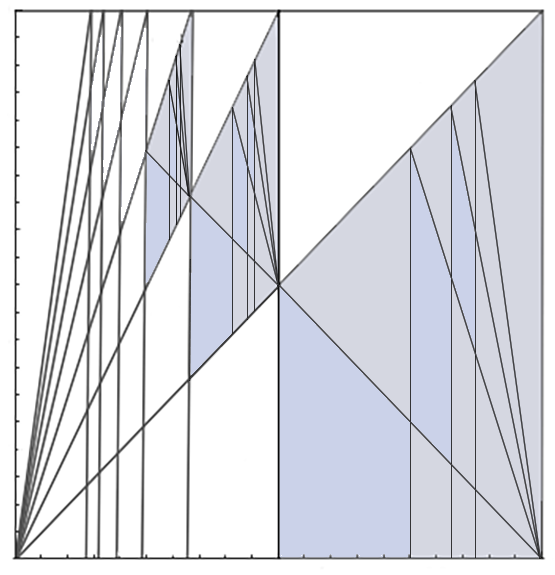
Figure 3. The sets $E_{3}^{(1)}$ and $E_{3}^{(2)}$, depicted in grey and blue, respectively.

Lemma 6.1 (Bounded distortion).

There exists a uniform constant $L>0$ so that for any $(a,b)\in{\mathcal{A}}^{n}$ with $n\geq 1$ and for any $(x_{1},y_{1})$ and $(x_{2},y_{2})$ in $I^{2}$, we have

$$\frac{1}{L}\leq\left|\frac{{\mathbf{J}}_{{\mathbf{h}}_{a,b}}(x_{1},y_{1})}{{\mathbf{J}}_{{\mathbf{h}}_{a,b}}(x_{2},y_{2})}\right|\leq L,$$

where $|{\mathbf{J}}_{{\mathbf{h}}_{a,b}}(x,y)|$ stands for the Jacobian (determinant) $|{\mathbf{J}}_{{\mathbf{h}}_{a,b}}(x,y)|$ of the inverse branch ${\mathbf{h}}_{a,b}$.

Proof.

According to the notation of Proposition 2.7, one has

$$|{\mathbf{J}}_{{\mathbf{h}}_{a,b}}(x,y)|=\frac{1}{(q_{n}+xq_{n-1})^{3}}$$

which does not depend on the skew coordinate $y$. We deduce the result directly from this expression, by taking e.g. $L=8$. ∎

Note that there is no Markov condition to consider here ($b$ is never equal to $a$). In order to study the Hausdorff dimension of $E_{N}$, one has to take suitable open covers. As classically done in the continued fraction setting, they will be based on fundamental sets. Hence, for any $(a,b)\in{\mathcal{A}}_{N}^{n}$, we consider the fundamental depth $n$ cylinder $I_{a,b}$, i.e., ${\mathbf{h}}_{a_{1},b_{1}}\circ\cdots\circ{\mathbf{h}}_{a_{n},b_{n}}(I^{2})$, which is simply a trapezium (we use here the fact that the digits $b_{i}$ are distinct from $a_{i}$ for all $i$). The fact that we have explicit estimates (by Proposition 2.7) for describing the fundamental sets of depth $n$ is crucial.

Together with the spectral properties from §4, we aim to get Bowen–Ruelle type estimates for the bounded-type set $E_{N}$. Here, we consider $w=0$, so we write ${\mathcal{L}}_{N,s}:={\mathcal{L}}_{N,s,0}$, for short, for the constrained operator deduced by the specialisation $\kappa$ from the operator ${\widetilde{\mathcal{L}}}_{N,s}=({\widetilde{\mathcal{L}}}_{0,(N,s)},{\widetilde{\mathcal{L}}}_{1,(N,s)})$, whose summand is restricted to ${\mathcal{A}}_{N}$, i.e., for $i\in\{0,1\}$

$${\widetilde{\mathcal{L}}}_{i,(N,s)}\Phi(x,y)=\sum_{j\in\{0,1\}}\sum_{(a,b)\in A_{N,i,j}}\frac{1}{(a+x)^{3s}}\cdot\Phi_{j}\left(\frac{1}{a+x},\frac{b+y}{a+x}\right)$$

where

$${\mathcal{A}}_{N,i,j}=\{(a,b)\in{\mathcal{A}}_{N}:{\mathbf{h}}_{a,b}({\Delta_{i}})\subset\Delta_{j}\}.$$

The constrained operator ${\mathcal{L}}_{N,s}$ has a spectral gap with the dominant eigenvalue $\lambda_{N,s}$ as the proof goes the same as Theorem 4.7.

Recall the fact that

$$E_{N}=\cap_{n\geq 1}\cup_{(a,b)\in{\mathcal{A}}_{N}^{n}}I_{a,b}$$

from (6.1) and consider open neighborhoods containing fundamental sets $I_{a,b}$ which form an open cover for $E_{N}$. The approach is similar to the one classically performed for regular continued fractions, such as developed in Jarnik [31], Good [24], or Fan–Liao–Wang–Wu [22], for instance. We now obtain the following upper bound.

Proposition 6.2.

We have $\dim_{H}E_{N}\leq\min\{s_{2},3s_{1}\},$ for $s_{1}$ satisfying $\lambda_{N,s_{1}}=1$ and $s_{2}$ satisfying $(N+1)^{2s_{2}}\lambda_{N,s_{2}}=1$.

Proof.

We fix $n$ and some point $(x,y)\in E_{N}$. First note that

$$({\mathcal{L}}^{n}_{N,s}\mathbf{1})(x,y)=\sum_{(a,b)\in{\mathcal{A}}_{N}^{n}}|{\mathbf{J}}_{a,b}(x,y)|^{s}$$

by taking the constant function $\mathbf{1}$. By the spectral gap property (see Remark 4.6), one has

$$|{\mathcal{L}}^{n}_{N,s}\mathbf{1}(x,y)-\lambda_{N,s}^{n}|\ll\lambda_{N,s}^{n}\rho^{n}$$

for some $\rho<1$. Also by Proposition 2.7 (and using the notation of its statement), one has $\mathrm{diam}(I_{a,b})\leq\frac{3}{q_{n}+q_{n-1}}$ and by Lemma 6.1, we have

$$|{\mathbf{J}}_{{\mathbf{h}}_{a,b}}(x,y)|\geq L^{-1}|{\mathbf{J}}_{{\mathbf{h}}_{a,b}}(0,0)|=L^{-1}\frac{1}{q_{n}}.$$

Hence for any $(a,b)\in{\mathcal{A}}_{N}^{n}$ and $(x,y)\in I^{2}$, this gives

$$\mathrm{diam}(I_{a,b})\leq C_{1}(N+1)^{2n}|{\mathbf{J}}_{{\mathbf{h}}_{a,b}}(x,y)|$$

for some $C_{1}>0$ by noticing that all $a_{i}$’s satisfy $a_{i}\leq N$, and then $q_{n}\leq(N+1)^{n}$. Accordingly, we get

$$\sum_{(a,b)\in{\mathcal{A}}_{N}^{n}}\mathrm{diam}(I_{a,b})^{s}\leq C_{1}^{s}(N+1)^{2ns}\sum_{(a,b)\in{\mathcal{A}}_{N}^{n}}|{\mathbf{J}}_{a,b}(x,y)|^{s}\leq C^{\prime}_{1}(N+1)^{2ns}\lambda_{N,s}^{n}$$

for some $C^{\prime}_{1}>0$. Taking the infimum over all open covers ${\mathcal{O}}$ whose elements have diameter at most $\delta$, we see that $\inf\sum_{O_{j}\in{\mathcal{O}}}\mathrm{diam}(O_{j})^{s}$ is bounded above by $C^{\prime}_{1}(N+1)^{2ns}\lambda_{N,s}^{n}$, where $n$ is chosen such that $\delta\geq\max_{{\mathcal{A}}_{N}^{n}}\mathrm{diam}(I_{a,b})$. This shows that if $(N+1)^{2s}\lambda_{N,s}<1$, then this infimum tends to 0 as $\delta$ goes to 0. Hence, we have $\dim_{H}(E_{N})\leq s_{2}$ for $s_{2}$ for which $(N+1)^{2s_{2}}\lambda_{N,s_{2}}=1$.

Similarly, Lemma 6.1 together with Proposition 2.7 gives, for some $C_{2},C^{\prime}_{2}>0$,

$$\sum_{(a,b)\in{\mathcal{A}}_{N}^{n}}\mathrm{diam}(I_{a,b})^{3s}\leq C_{2}^{3s}\sum_{(a,b)\in{\mathcal{A}}_{N}^{n}}\mathrm{Jac}(I_{a,b})^{s}\leq(C_{2}^{\prime})^{s}\lambda_{N,s}^{n},$$

we also obtain $\dim_{H}E_{N}\leq 3s_{1}$ for $s_{1}$ satisfying $\lambda_{N,s_{1}}=1$. ∎

For the lower bound, we further observe:

Proposition 6.3.

We have $\frac{3s_{1}}{2}\leq dim_{H}E_{N}$ for $s_{1}$ satisfying $\lambda_{N,s_{1}}=1$.

Proof.

We consider the Gibbs measure $\mu_{N,s}$ defined as the probability eigenmeasure of $\lambda_{N,s}$ for the dual operator of the constrained operator ${\mathcal{L}}_{N,s}$, whose existence is given by the analogue of Theorem 4.7 for the constrained operator. It satisfies, with some constant $C_{3}$, for $(a,b)\in{\mathcal{A}}_{N}^{n}$ and for some fixed $(x,y)\in E_{N}$, by also Lemma 6.1:

(6.2) $$\mu_{N,s}(I_{a,b})=\lambda_{N,s}^{-n}\int_{I^{2}}({\mathcal{L}}_{N,s}^{n}\mathbf{1}_{I_{a,b}})d\mu_{N,s}\leq C_{3}\lambda_{N,s}^{-n}|{\mathbf{J}}_{{\mathbf{h}}_{a,b}}(x,y)|^{s}.$$

We now fix $s$ equal to $s_{1}$ with $\lambda_{N,s_{1}}=1$.

We use Notation 2.6 and Proposition 2.7. We recall from (6.1) that the set

$$E_{N}=\cap_{n\geq 1}\cup_{(a,b)\in{\mathcal{A}}_{N}^{n}}I_{a,b}$$

is the intersection of the sequence of decreasing subsets $\cup_{(a,b)\in{\mathcal{A}}_{N}}I_{n}(a_{1},\cdots,a_{n})$ for $(a,b)=((a_{1},a_{1}-1),\cdots,(a_{n},a_{n}-1))\in{\mathcal{A}}_{N}^{n}$. For given $(a_{1},\cdots,a_{n})$, we consider the natural decomposition (up to the boundaries of the atoms) as follows (see Figure 4 as an illustration):

(6.3) $$K_{n}(a_{1},\cdots,a_{n})=I_{n}(a_{1},\cdots,a_{n})\backslash\bigcup_{1\leq k\leq N}I_{n+1}(a_{1},\cdots,a_{n},k).$$

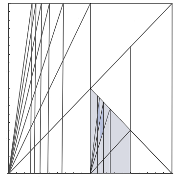
Figure 4. The set $K_{2}(1,1)$, depicted in blue, inside $I_{2}(1,1)$ ($N=2$).

Then the set $K_{n}(a_{1},\cdots,a_{n})$ is a union of fundamental sets $I_{a^{\prime},b^{\prime}}$ corresponding to elements $(a^{\prime},b^{\prime})\in{\mathcal{A}}^{n+1}$ satisfying $a^{\prime}_{1}=a_{1},\cdots,a^{\prime}_{n}=a_{n}$ and $a^{\prime}_{n+1}\geq N+1$, also $b^{\prime}_{1}=a_{1}-1,\cdots,b^{\prime}_{n}=a_{n}-1$ and $b^{\prime}_{n+1}\leq a^{\prime}_{n+1}$. The set $\bigcup_{1\leq k\leq N}I_{n+1}(a_{1},\cdots,a_{n},k)$ is a connected component of $I_{n}(a_{1},\cdots,a_{n})$ made of a finite union of trapeziums, and the trapezium $K_{n}(a_{1},\cdots,a_{n})$ is taken away from $I_{n}(a_{1},\cdots,a_{n})$ at level $n$ for defining $E_{N}$; we consider it as a “hole”. Notice that the hole is located on the right of $I_{n}(a_{1},\cdots,a_{n})$ if and and only if $n$ is odd.

Let $B(\delta)$ be a closed ball of radius $\delta$ in $E_{N}$. Let $n$ be the largest integer such that $B(\delta)\subset I_{n-1}(a_{1},\cdots,a_{n-1})$, for some $(a_{1},\cdots,a_{n-1})$. The ball $B(\delta)$ thus intersects at least two sets of the form $I_{n}(a_{1},\cdots,a_{n-1},k+1)$ and $I_{n}(a_{1},\cdots,a_{n-1},k)$ ($1\leq k\leq N-1$). We assume w.l.o.g. that $n$ is odd. This implies that the hole $K_{n-1}(a_{1},\cdots,a_{n-1})$ is on the left of $I_{n-1}(a_{1},\cdots,a_{n-1})$, and thus that the set $I_{n}(a_{1},\cdots,a_{n-1},k+1)$ is located on the left of $I_{n}(a_{1},\cdots,a_{n-1},k)$. Moreover, the hole $K_{n}(a_{1},\cdots,a_{n-1},k+1)$ is on the right of $I_{n}(a_{1},\cdots,a_{n-1},k+1)$. Since $B(\delta)$ intersects $I_{n}(a_{1},\cdots,a_{n-1},k+1)$ and $I_{n}(a_{1},\cdots,a_{n-1},k)$, then $\delta$ is larger than the difference of the lower vertices of the set $K_{n}(a_{1},\cdots,a_{n-1},k+1)$.

It remains to determine the lower vertices of $K_{n}(a_{1},\cdots,a_{n-1},k+1)$. The fundamental set $I_{n+1}(a_{1},\cdots,a_{n-1},k+1,N)$ is located just on the left of the hole $K_{n}(a_{1},\cdots,a_{n-1},k+1)$ within the fundamental set $I_{n}(a_{1},\cdots,a_{n-1},k+1)$. According to Notation 2.6, the right lower vertex of $I_{n+1}(a_{1},\cdots,a_{n-1},k+1,N)$ is $D_{n+1}(a_{1},\cdots,a_{n-1},k+1,N)$. This gives that the left lower vertex of the hole $K_{n}(a_{1},\cdots,a_{n-1},k+1)$ is $D_{n+1}(a_{1},\cdots,a_{n-1},k+1,N)$. The right lower vertex of the hole $K_{n}(a_{1},\cdots,a_{n-1},k+1)$ is the right lower vertex of $I_{n}(a_{1},\cdots,a_{n-1},k+1)$, namely $A_{n}(a_{1},\cdots,a_{n-1},k+1)$. The lower vertices of $K_{n}(a_{1},\cdots,a_{n-1},k+1)$ are thus $D_{n+1}(a_{1},\cdots,a_{n-1},k+1,N)$ and $A_{n}(a_{1},\cdots,a_{n-1},k=1)$. Hence $\delta$ is larger than the absolute value of the difference of their abcisses, denoted by $|-D_{n+1}(a_{1},\cdots,a_{n-1},k+1,N)+A_{n}(a_{1},\cdots,a_{n-1},k+1)|_{x}$.

Now, let us prove that $\delta\geq\frac{1}{(N+1)^{3}q_{n-1}^{2}}.$ By Proposition 2.7, one has

$$|-D_{n+1}(a_{1},\cdots,a_{n-1},k+1, N)+A_{n}(a_{1},\cdots,a_{n-1},k+1))|_{x}$$

$$=\frac{p_{n+1}+p_{n}(k+1)}{q_{n+1}+q_{n}(k+1)}-\frac{p_{n}(k+1)}{q_{n}(k+1)}$$

by using the following notation:

$$p_{n+1}=p_{n+1}(a_{1},\cdots,a_{n-1},k+1,N),\ p_{n}(k+1)=p_{n}(a_{1},\cdots,a_{n-1},k+1),$$

$$p_{n-1}=p_{n-1}(a_{1},\cdots,a_{n-1}),$$

with also the analogous notation for the $q_{n}$’s. One has $q_{n}(k+1)=q_{n}(k)+q_{n-1},$ and similarly for the $p_{n}$’s. This gives

$$\delta\geq\left|\frac{p_{n+1}+p_{n}(k+1)}{q_{n+1}+q_{n}(k+1)}-\frac{p_{n}(k+1)}{q_{n}(k+1)}\right|=\frac{1}{(q_{n+1}+q_{n}(k+1))q_{n}(k+1)}\geq\frac{1}{(N+1)^{3}q_{n-1}^{2}}$$

by noticing that $q_{n}(k+1)\leq(N+1)q_{n-1}$ and $q_{n+1}\leq(N^{2}+N+1)q_{n-1}\leq(N+1)^{2}q_{n-1}$.

Moreover, there is a positive integer $\ell$ such that for all $m$ and for any $\ell+m$-tuple $(a^{\prime},b^{\prime})$ of pairs of digits in ${\mathcal{A}}_{N}^{\ell+m}$, one has

$$\frac{1}{q_{m+\ell}(a^{\prime},b^{\prime})}\leq\frac{1}{(N+1)^{3/2}q_{m-1}(a^{\prime},b^{\prime})}\leq\delta^{1/2},$$

(here the dependence of the $q_{i}$’s with respect to the choice of digits $(a^{\prime},b^{\prime})$ is denoted as $q_{i}(a^{\prime},b^{\prime})$). Hence, by setting $m=n$, Proposition 2.7 yields that the corresponding Jacobian ${\mathbf{J}}_{{\mathbf{h}}_{a^{\prime},b^{\prime}}}$ satisfies

$$|{\mathbf{J}}_{{\mathbf{h}}_{a^{\prime},b^{\prime}}}|\leq\frac{1}{q_{n+\ell}^{3}(a^{\prime},b^{\prime})}\leq\delta^{3/2}.$$

Since $B(\delta)\subset I_{n-1}(a_{1},\cdots,a_{n-1})$, $B(\delta)$ is covered by at most $N^{\ell+1}$ cylinders of depth $n+\ell$, and by (6.2), one has

$$\mu_{N,s_{1}}(B(\delta))\leq C_{3}N^{\ell+1}\delta^{3s_{1}/2}.$$

Thus by mass distribution principle, we get $\dim_{H}(E_{N})\geq 3s_{1}/2$. ∎

We end with one final observation by discussing a simple corollary following Hensley [28]. Indeed, together with the spectral gap from Theorem 4.7 and 4.4, the following relation between the leading eigenvalues of ${\mathcal{L}}_{N,s}$ and ${\mathcal{L}}_{s}$, namely

(6.4) $$\lambda_{N,1-\frac{s}{N}}=\lambda_{1-\frac{s}{N}}+O(N^{-1}),$$

is an almost straightforward adaptation of the arguments due to Hensley. Remark that Hensley [28] obtain this more precisely with an accurate $N^{-1}$ order term and $O(N^{-2})$, but here we only consider a simple situation.

Looking at the Taylor expansion at $s=0$, we have

(6.5) $$\lambda_{1-\frac{s}{N}}=1-\frac{s}{N}\cdot\frac{d}{ds}\lambda_{s}\Big{|}_{s=1}+O(N^{-2}).$$

This shows that if one gets the first derivative of $\lambda_{s}$ of ${\mathcal{L}}_{s}$, then it is possible to calculate the eigenvalue $\lambda_{N,s}$ of the constrained operator ${\mathcal{L}}_{N,s}$.

Consider now the operator

$${\mathcal{A}}\phi(x,y)=-\sum_{(a,b)\in{\mathcal{A}}}\frac{3\log(a+x)}{(a+x)^{3}}\cdot\phi\left(\frac{1}{a+x},\frac{b+y}{a+x}\right).$$

Note that this operator is simply defined by ${\mathcal{A}}\phi=\frac{d}{ds}{\mathcal{L}}_{s}\Big{|}_{s=1}$ and thus it satisfies

(6.6) $${\mathcal{L}}_{s}={\mathcal{L}}_{1}+(s-1){\mathcal{A}}+O(|s-1|^{2})$$

where $s$ is close to 1. Here by the decomposition theory of bounded operators (see Hensley [28, Lemma 7]), for the invariant density $\varphi_{*}$ from Remark 4.5, we can write ${\mathcal{A}}\varphi_{*}=c\varphi_{*}+\eta$ for some $c\in{\mathbb{C}}$ with $\eta$ belonging to the image of ${\mathcal{A}}-cI$. Evaluating the projection operator, we have $\mathcal{P}{\mathcal{A}}\varphi_{*}=c\varphi_{*}$ since $\mathcal{P}\circ\eta=0$. Thus from integral representation for $\mathcal{P}$, we see that $c=\int_{I^{2}}{\mathcal{A}}\varphi_{*}dm$. We first claim that $c=\frac{d}{ds}\lambda_{s}|_{s=1}$. Set $z=s-1$ and $u=(I-{\mathcal{L}}_{1})^{-1}\eta$, then (6.6) gives

$${\mathcal{L}}_{s}(\varphi_{*}+zu) ={\mathcal{L}}_{1}(\varphi_{*}+zu)+z{\mathcal{A}}(\varphi_{*}+zu)+O(|z|^{2})$$

$$=(\varphi_{*}+zu)+cz(\varphi_{*}+zu)+O(|z|^{2})$$

since we have $\lambda_{1}=1$. Hence for $|z|$ being sufficiently small, by perturbation theory (see e.g. [28, §6]), this yields that $|\lambda_{s}-(1+cz)|\ll|z|^{2}$ and thus $\frac{d}{ds}\lambda_{s}|_{s=1}=c$.

Therefore we have

$$c=\frac{d}{ds}\lambda_{s}\Big{|}_{s=1} =\int_{I^{2}}{\mathcal{A}}\varphi_{*}(x,y)d(x,y)$$

$$=-\frac{1}{2\log 2}\int_{0}^{1}\sum_{a\geq 1}(a+1)x\cdot\frac{3\log(a+x)}{(a+x)^{3}}\cdot\frac{(3a+1)+3x}{(a+x)^{2}((a+1)+x)^{2}}dx$$

$$\ \ \ \ \ \ \ +\frac{1}{2\log 2}\int_{0}^{1}\sum_{a\geq 1}a(1-x)\cdot\frac{3\log(a+x)}{(a+x)^{3}}\cdot\frac{(2a+1)+2x}{(a+x)^{2}((a+1)+x)^{2}}dx.$$

Together with (6.4) and (6.5), we have $\lambda_{N,1-\frac{s}{N}}=1-c\cdot\frac{s}{N}+O(N^{-2})$.

Remark 6.4.

Proposition 6.2 and 6.3 show that the Hausdorff dimension of $E_{N}$ can be estimated via the bounded distortion property of the Jacobian as an application of the spectral analysis of the transfer operator due to nice properties of the Ostrowski dynamical system, despite the non-conformality. Though this is far from being sufficient to have the same upper and lower bound. We even expect both bounds not being sharp, the upper bound being in particuar far from optimal, which we plan to investigate in the further work.

7. Appendix

7.1. Proof of Proposition 2.7

Let $(a,b)=((a_{1},b_{1}),\ldots,(a_{n},b_{n}))\in{\mathcal{A}}^{n}$. We keep the notation of Proposition 2.7 for the definition of $(p_{k})_{-1\leq k\leq n}$ and $(q_{k})_{-1\leq k\leq n}$. The matrix of the homography ${\mathbf{h}}_{a,b}$ is $M_{a_{1},b_{1}}\cdots M_{a_{n},b_{n}}$, where $M_{a_{i},b_{i}}:=\begin{bmatrix}0&0&1\\ 0&1&b_{i}\\ 1&0&a_{i}\end{bmatrix}.$ It is thus of the form

$$\begin{bmatrix}p_{n-1}&0&p_{n}\\ \alpha_{n-1}&1&\alpha_{n}\\ q_{n-1}&0&q_{n}\end{bmatrix}$$

with

(7.1) $$\alpha_{n}=\sum_{i=1}^{n}b_{i}(-1)^{i}(q_{n}p_{i-1}-p_{n}q_{i-1})=\sum_{i=1}^{n}b_{i}|q_{n}p_{i-1}-p_{n}q_{i-1}|.$$

Note that the expressions for $\alpha_{n}$ can be obtained by induction, with the induction relation being $\alpha_{k+1}=\alpha_{k-1}+b_{k+1}+\alpha_{k}a_{k+1}$, by observing that the sign of $q_{n}p_{i-1}-p_{n}q_{i-1}$ is given by $(-1)^{i}$ ($1\leq i\leq n-1$) and thus does not depend on $n$. We directly deduce from this expression the first statement on the Jacobian.

The set $I_{a,b}$ is either equal to ${\mathbf{h}}_{a,b}(I^{2})$ or ${\mathbf{h}}_{a,b}(\Delta_{0})$. According to Notation 2.5 and from the expression ${\mathbf{h}}_{a,b}(x,y)=(\frac{p_{n-1}x+p_{n}}{q_{n-1}x+q_{n}},\frac{\alpha_{n-1}x+y+\alpha_{n}}{q_{n-1}x+q_{n}}),$ one deduces that the vertices of $I_{a,b}$ belong to the set $A_{n}={\mathbf{h}}_{a,b}(0,0)$, $B_{n}={\mathbf{h}}_{a,b}(0,1)$, $C_{n}={\mathbf{h}}_{a,b}(1,1)$, and $D_{n}={\mathbf{h}}_{a,b}(1,0)$, with

$$A_{n} =\left(\frac{p_{n}}{q_{n}},\frac{\alpha_{n}}{q_{n}}\right),\ B_{n}=\left(\frac{p_{n}}{q_{n}},\frac{\alpha_{n}+1}{q_{n}}\right),$$

$$C_{n} =\left(\frac{p_{n}+p_{n-1}}{q_{n}+q_{n-1}},\frac{\alpha_{n}+\alpha_{n-1}+1}{q_{n}+q_{n-1}}\right),\ D_{n}=\left(\frac{p_{n}+p_{n-1}}{q_{n}+q_{n-1}},\frac{\alpha_{n}+\alpha_{n-1}}{q_{n}+q_{n-1}}\right).$$

Let $K_{n}$ stand for the maximum of the absolute values of the cofactors of the matrix of ${\mathbf{h}}_{a,b}$. One checks that the diameter of $I_{a,b}$ is smaller than or equal to $3K_{n}/q_{n}^{2}$. One has

$$K_{n}=\max(|-p_{n}\alpha_{n-1}+\alpha_{n}p_{n-1}|,|-q_{n}\alpha_{n-1}+\alpha_{n}q_{n-1}|,1,p_{n},q_{n},p_{n-1},q_{n-1}).$$

Moreover, one deduces from (7.1) that, for any positive $n$,

(7.2) $$-q_{n}\alpha_{n-1}+\alpha_{n}q_{n-1}=\sum_{i=1}^{n}b_{i}(-1)^{n+i}q_{i-1},$$

and similarly $-p_{n}\alpha_{n-1}+\alpha_{n}p_{n-1}=\sum_{i=1}^{n}b_{i}(-1)^{n+i}p_{i-1}.$ This implies that $K_{n}=q_{n}$ and thus that the diameter of $I_{a,b}$ is in $O(1/q_{n})$.

Now we assume that $(a,b)\in{\mathcal{A}}_{N}^{n}$. We will get more precise estimates in this case. We have $I_{a,b}={\mathbf{h}}_{a,b}(I^{2})$. In particular $I_{a,b}$ is quadrangular (and not triangular). The measure of $I_{a,b}$ thus satisfies

$$\int_{I^{2}}\left(\frac{1}{q_{n}+xq_{n-1}}\right)^{3}dxdy=\int_{[0,1]}\left(\frac{1}{q_{n}+xq_{n-1}}\right)^{3}dx=\frac{q_{n-1}+2q_{n}}{2q_{n}^{2}(q_{n}+q_{n-1})^{2}}.$$

We recall that the four vertices of $I_{a,b}$ are denoted by $A_{n}={\mathbf{h}}_{a,b}(0,0)$, $B_{n}={\mathbf{h}}_{a,b}(0,1)$, $C_{n}={\mathbf{h}}_{a,b}(1,1)$, and $D_{n}={\mathbf{h}}_{a,b}(1,0)$. The trapezium $I_{a,b}$ is inscribed in a rectangle with parallel vertical sides of width $\frac{1}{q_{n}(q_{n}+q_{n-1})}$. One has $B_{n}$ above $A_{n}$ and $C_{n}$ above $D_{n}$. Its two sides have respective lengths $\frac{1}{q_{n}}$ and $\frac{1}{q_{n}+q_{n-1}}$. Hence the diameter of this quadrangular is bounded below by $\frac{1}{q_{n}+q_{n-1}}$.

One has

$$\sum_{i=1}^{n}(-1)^{i}a_{i}q_{i-1}=(-1)^{n}(q_{n}-q_{n-1})-q_{0}+q_{-1}=(-1)^{n}(q_{n}-q_{n-1})-1,$$

which gives

(7.3) $$\sum_{i=1}^{n}(-1)^{i}(a_{i}-1)q_{i-1}=(-1)^{n}(q_{n}-2q_{n-1})+\sum_{i=1}^{n-2}(-1)^{i}q_{i}.$$

Hence by (7.2) and (7.3), this gives

$$-q_{n}\alpha_{n-1}+\alpha_{n}q_{n-1}=q_{n}-2q_{n-1}+(-1)^{n}\sum_{i=1}^{n-2}(-1)^{i}q_{i}.$$

For two points $A$ and $B$, the notation $(A-B)_{y}$ stands for the difference between their coordinates. We have

$$(C_{n}-A_{n})_{y}=\frac{-\alpha_{n}q_{n-1}+\alpha_{n-1}q_{n}+q_{n}}{q_{n}(q_{n}+q_{n-1})}.$$

Hence by (7.2) and (7.3), one gets

$$(C_{n}-A_{n})_{y}=\frac{\sum_{i=1}^{n}b_{i}(-1)^{n+i}q_{i-1}+q_{n}}{q_{n}(q_{n}+q_{n-1})}=\frac{2q_{n}-2q_{n-1}+(-1)^{n}\sum_{i=1}^{n-2}(-1)^{i}q_{i}}{q_{n}(q_{n}+q_{n-1})},$$

which implies

$$0<(C_{n}-A_{n})_{y}<\frac{2}{q_{n}+q_{n-1}}.$$

Similarly, one has

$$(B_{n}-D_{n})_{y}=\frac{\alpha_{n}q_{n-1}-\alpha_{n-1}q_{n}+q_{n}+q_{n-1}}{q_{n}(q_{n}+q_{n-1})},$$

which gives

$$0<(B_{n}-D_{n})_{y}=\frac{2q_{n}-q_{n-1}+(-1)^{n}\sum_{i=1}^{n-2}(-1)^{i}q_{i}}{q_{n}(q_{n}+q_{n-1})}<\frac{2}{q_{n}+q_{n-1}}.$$

7.2. Proof of Proposition 2.1

Proof of Proposition 2.1.

We follow here mainly the proof given in [9].

We first state some useful identities. Recall that $|\theta_{k-1}|=a_{k+1}|\theta_{k}|+|\theta_{k+1}|$ ($k\geq 0$). Further, we have $\theta_{-1}=1$ and $\theta_{0}=x$. We also recall that the series $\sum_{k=0}^{\infty}a_{k}|\theta_{k}|$ is convergent as established in §2.1, and that $\sum_{k=n}^{\infty}a_{k}|\theta_{k-1}|=|\theta_{n-2}|+|\theta_{n-1}|$ holds for all positive $n$ (by (2.3)). By using telescoping sums, one gets

$$1+x=\sum_{k=1}^{\infty}a_{k}|\theta_{k-1}|,\quad 1-x=\sum_{k=1}^{\infty}a_{k}\theta_{k-1}$$

which gives

(7.4) $$x=\sum_{k=1}^{\infty}a_{2k}|\theta_{2k-1}|,\quad 1=\sum_{k=0}^{\infty}a_{2k+1}|\theta_{2k}|.$$

We first show that the sequence of digits $(a_{i},b_{i})_{i\geq 1}$ produced by the Ostrowski map applied to $(x,y)$ satisfies the admissibility conditions (1–3). Recall that $a_{i}=\lfloor\frac{1}{x_{i-1}}\rfloor$ and $b_{i}=\lfloor\frac{y_{i-1}}{x_{i-1}}\rfloor$ ($i\geq 1$). Since $y<1$, we have $\lfloor\frac{y_{i-1}}{x_{i-1}}\rfloor\leq\lfloor\frac{1}{x_{i-1}}\rfloor$, which yields (1). Assume that $a_{i}=b_{i}$. One has $x_{i}=\frac{1}{x_{i-1}}-a_{i}$, and $y_{i}=\frac{x_{i-1}}{y_{i-1}}-b_{i}$. One has $y_{i}<x_{i}$, since $\frac{y_{i-1}}{x_{i-1}}<\frac{1}{x_{i-1}}$ and $a_{i}=b_{i}$. This implies that $b_{i+1}=\lfloor\frac{y_{i}}{x_{i}}\rfloor=0$, which gives (2). Finally we claim (3). One has $y=\sum_{i=1}^{\infty}b_{i}|\theta_{i-1}|$. Assume that $a_{i}=b_{i}$ for all odd integer greater than some $i_{0}\geq 1$. In particular, by Condition (2), $b_{i}=0$ for all even index larger than $i_{0}$. Applying Ostrowski’s map $S$ to $(x_{i_{0}-1},y_{i_{0}-1})$ gives the expansion $(a_{i},b_{i})_{i\geq i_{0}}$. This implies by (7.4) that $1=\sum_{i\geq i_{0}}^{\infty}a_{i}|\theta_{i-1}|=y_{i_{0}}<1,$ which yields the desired contradiction. The same reasoning applies for the case of even indices.

We now prove the uniqueness of the expansion. Let us fix $y\in[0,1)$. Let $(b_{i})_{i\geq 1}$ and $(b^{\prime}_{i})_{i\geq 1}$ be such that

$$y=\sum_{i=1}^{\infty}b_{i}|\theta_{i-1}|=\sum_{i=1}^{\infty}b^{\prime}_{i}|\theta_{i-1}|$$

where $0\leq b_{i}\leq a_{i}$ for all $i\geq 1$, $b_{i+1}=0$ if $a_{i}=b_{i}$, $b_{i}\neq a_{i}$ for infinitely many even and odd integers, and the same assumptions for $(b^{\prime}_{i})_{i\geq 1}$. Suppose that $(b_{i})_{i}\neq(b^{\prime}_{i})_{i}$. Let $k$ be the smallest positive integer $i$ such that $b_{i}\neq b^{\prime}_{i}$. We assume without loss of generality that $b_{k}>b^{\prime}_{k}$. Then one has

$$\sum_{i=k+1}^{\infty}(b^{\prime}_{i}-b_{i})|\theta_{i-1}|=\sum_{i=1}^{k}(b_{i}-b^{\prime}_{i})|\theta_{i-1}|=(b_{k}-b^{\prime}_{k})|\theta_{k-1}|\geq|\theta_{k-1}|.$$

• First assume that $(b^{\prime}_{k+1}-b_{k+1})\leq a_{k+1}-1$. By (2.3) and since $b^{\prime}_{i}\neq a^{\prime}_{i}$ for infinitely many $i$, one has

  $$\sum_{i\geq k+2}(b^{\prime}_{i}-b_{i})|\theta_{i-1}|<|\theta_{k}|+|\theta_{k+1}|.$$

  Hence we get

  $$|\theta_{k-1}|\leq\sum_{i\geq k+1}(b^{\prime}_{i}-b_{i})|\theta_{i-1}|<a_{k+1}|\theta_{k}|+|\theta_{k+1}|=|\theta_{k-1}|,$$

  which gives a contradiction.

• We now assume that $b^{\prime}_{k+1}-b_{k+1}=a_{k+1}$. This implies that $b_{k+1}=0$, $b^{\prime}_{k+1}=a_{k+1}$ and consequently $b^{\prime}_{k+2}=0$. Let $\ell$ be the smallest positive integer such that $b^{\prime}_{k+1+2\ell}-b_{k+1+2\ell}<a_{k+1+2\ell}$ (such an index exists since $b^{\prime}_{i}\neq a_{i}$ for infinitely many even and odd integers). One has again by (2.3), and since $b^{\prime}_{i}\neq a_{i}$ for infinitely many $i$,

  $$\sum_{i\geq k+2\ell+2}(b^{\prime}_{i}-b_{i})|\theta_{i-1}|<|\theta_{k+2\ell}|.$$

  Consequently, one has

  $$|\theta_{k-1}|\leq\sum_{i\geq k+1}(b^{\prime}_{i}-b_{i})|\theta_{i-1}| =\sum_{i=0}^{\ell-1}a_{k+1+2i}|\theta_{k+2i}|+\sum_{i\geq k+2\ell+1}(b^{\prime}_{i}-b_{i})|\theta_{i-1}|$$

  $$<\sum_{i=1}^{\ell-1}a_{k+1+2i}|\theta_{k+2i}|+|\theta_{k+2\ell}|\leq|\theta_{k-1}|,$$

  which yields the desired contradiction, by noticing that

  $$\sum_{i=0}^{\ell-1}a_{k+1+2i}|\theta_{k+2i}|+|\theta_{k+2\ell}|=|\theta_{k-1}|.$$

∎

References

- [1] P. Arnoux and A. M. Fisher. The scenery flow for geometric structures on the torus: the linear setting. Chinese Ann. Math. Ser. B, 22(4):427–470, 2001.
- [2] A. Avila, P. Hubert, and A. Skripchenko. On the Hausdorff dimension of the Rauzy gasket. Bull. Soc. Math. France, 144(3):539–568, 2016.
- [3] V. Baladi. Dynamical zeta functions and dynamical determinants for hyperbolic maps, volume 68 of Ergebnisse der Mathematik und ihrer Grenzgebiete. 3. Folge. A Series of Modern Surveys in Mathematics. Springer, Cham, 2018. A functional approach.
- [4] V. Baladi and B. Vallée. Euclidean algorithms are Gaussian. J. Number Theory, 110(2):331–386, 2005.
- [5] G. Barat and P. Liardet. Dynamical systems originated in the Ostrowski alpha-expansion. Ann. Univ. Sci. Budapest. Sect. Comput., 24:133–184, 2004.
- [6] V. Beresnevich, A. Haynes, and S. Velani. Sums of reciprocals of fractional parts and multiplicative Diophantine approximation. Mem. Amer. Math. Soc., 263(1276):vii + 77, 2020.
- [7] V. Berthé. Autour du système de numération d’Ostrowski. Bull. Belg. Math. Soc. Simon Stevin, 8(2):209–239, 2001.
- [8] V. Berthé and L. Imbert. Diophantine approximation, Ostrowski numeration and the double-base number system. Discrete Math. Theor. Comput. Sci., 11(1):153–172, 2009.
- [9] A. Bourla. The ostrowski expansions revealed, 2016.
- [10] R. Bowen. Hausdorff dimension of quasicircles. Inst. Hautes Études Sci. Publ. Math., (50):11–25, 1979.
- [11] A. Broise. Fractions continues multidimensionnelles et lois stables. Bull. Soc. Math. France, 124(1):97–139, 1996.
- [12] A. Broise. Transformations dilatantes de l’intervalle et théorèmes limites. In Astérisque, number 238, pages 1–109. 1996. Études spectrales d’opérateurs de transfert et applications.
- [13] M. Bromberg and C. Ulcigrai. A temporal central limit theorem for real-valued cocycles over rotations. Ann. Inst. Henri Poincaré Probab. Stat., 54(4):2304–2334, 2018.
- [14] Y. Bugeaud, S. Harrap, S. Kristensen, and S. Velani. On shrinking targets for actions on tori. Mathematika, 56(2):193–202, 2010.
- [15] Y. Bugeaud, D. H. Kim, S. Lim, and M. Rams. Hausdorff dimension in inhomogeneous Diophantine approximation. Int. Math. Res. Not. IMRN, (3):2108–2133, 2021.
- [16] Y. Bugeaud and Z. Zhang. On homogeneous and inhomogeneous Diophantine approximation over the fields of formal power series. Pacific J. Math., 302(2):453–480, 2019.
- [17] J. W. S. Cassels. Über . Math. Ann., 127:288–304, 1954.
- [18] E. Cesaratto and B. Vallée. Hausdorff dimension of real numbers with bounded digit averages. Acta Arith., 125(2):115–162, 2006.
- [19] T. W. Cusick, A. M. Rockett, and P. Szüsz. On inhomogeneous Diophantine approximation. J. Number Theory, 48(3):259–283, 1994.
- [20] T. Das, L. Fishman, D. Simmons, and M. Urbański. Hausdorff dimensions of perturbations of a conformal iterated function system via thermodynamic formalism. arXiv:2007.10554, 2020.
- [21] R. Descombes. Sur la répartition des sommets d’une ligne polygonale régulière non fermée. Ann. Sci. Ecole Norm. Sup. (3), 73:283–355, 1956.
- [22] A.-H. Fan, L.-M. Liao, B.-W. Wang, and J. Wu. On Khintchine exponents and Lyapunov exponents of continued fractions. Ergodic Theory Dynam. Systems, 29(1):73–109, 2009.
- [23] C. Fougeron. Dynamical properties of simplicial systems and continued fraction algorithms. arXiv:2001.01367, 2020.
- [24] I. J. Good. The fractional dimensional theory of continued fractions. Proc. Cambridge Philos. Soc., 37:199–228, 1941.
- [25] R. Gutiérrez-Romo and C. Matheus. Lower bounds on the dimension of the Rauzy gasket. Bull. Soc. Math. France, 148(2):321–327, 2020.
- [26] Y. Hara and S. Ito. On real quadratic fields and periodic expansions. Tokyo J. Math., 12(2):357–370, 1989.
- [27] D. Hensley. The Hausdorff dimensions of some continued fraction Cantor sets. J. Number Theory, 33(2):182–198, 1989.
- [28] D. Hensley. Continued fraction Cantor sets, Hausdorff dimension, and functional analysis. J. Number Theory, 40(3):336–358, 1992.
- [29] S. Ito. Some skew product transformations associated with continued fractions and their invariant measures. Tokyo J. Math., 9(1):115–133, 1986.
- [30] S. Ito and H. Nakada. Approximations of real numbers by the sequence and their metrical theory. Acta Math. Hungar., 52(1-2):91–100, 1988.
- [31] V. Jarnik. Zur Theorie der diophantischen Approximationen. Monatsh. Math. Phys., 39(1):403–438, 1932.
- [32] O. Jenkinson, L. F. Gonzalez, and M. Urbański. On transfer operators for continued fractions with restricted digits. Proc. London Math. Soc. (3), 86(3):755–778, 2003.
- [33] O. Jenkinson and M. Pollicott. Rigorous effective bounds on the Hausdorff dimension of continued fraction Cantor sets: a hundred decimal digits for the dimension of . Adv. Math., 325:87–115, 2018.
- [34] T. Kato. Perturbation theory for linear operators. Classics in Mathematics. Springer-Verlag, Berlin, 1995. Reprint of the 1980 edition.
- [35] A. Khintchine. Neuer Beweis und Verallgemeinerung eines Hurwitzschen Satzes. Math. Ann., 111(1):631–637, 1935.
- [36] D. H. Kim. The shrinking target property of irrational rotations. Nonlinearity, 20(7):1637–1643, 2007.
- [37] D. H. Kim and L. Liao. Dirichlet uniformly well-approximated numbers. Int. Math. Res. Not., (24):7691–7732, 2019.
- [38] M. A. Krasnoselskiĭ. Positive solutions of operator equations. P. Noordhoff Ltd. Groningen, 1964. Translated from the Russian by Richard E. Flaherty; edited by Leo F. Boron.
- [39] J. C. Lagarias. The quality of the Diophantine approximations found by the Jacobi-Perron algorithm and related algorithms. Monatsh. Math., 115(4):299–328, 1993.
- [40] S. Lim, N. de Saxcé, and U. Shapira. Dimension bound for badly approximable grids. Int. Math. Res. Not. IMRN, (20):6317–6346, 2019.
- [41] D. H. Mayer. Approach to equilibrium for locally expanding maps in . Comm. Math. Phys., 95(1):1–15, 1984.
- [42] H. Minkowski. Ueber die Annäherung an eine reelle Grösse durch rationale Zahlen. Math. Ann., 54(1-2):91–124, 1900.
- [43] M. Morse and G. A. Hedlund. Symbolic dynamics II. Sturmian trajectories. Amer. J. Math., 62:1–42, 1940.
- [44] D. Ruelle. Thermodynamic formalism, volume 5 of Encyclopedia of Mathematics and its Applications. Addison-Wesley Publishing Co., Reading, Mass., 1978. The mathematical structures of classical equilibrium statistical mechanics, With a foreword by Giovanni Gallavotti and Gian-Carlo Rota.
- [45] O. M. Sarig. Introduction to the transfer operator method. Winter school on dynamics, Hausdorff Research Institute for Mathematics, Bonn, 2020.
- [46] V. T. Sós. On the theory of Diophantine approximations. II. Inhomogeneous problems. Acta Math. Acad. Sci. Hungar., 9:229–241, 1958.
- [47] W. A. Veech. Interval exchange transformations. J. Analyse Math., 33:222–272, 1978.