Imaging Calibration of AstroSat Cadmium Zinc Telluride Imager (CZTI)

Imaging Calibration of AstroSat Cadmium Zinc Telluride Imager (CZTI)

Abstract

AstroSat is India’s first space-based astronomical observatory, launched on September 28, 2015. One of the payloads aboard AstroSat is the Cadmium Zinc Telluride Imager (CZTI), operating at hard X-rays. CZTI employs a two-dimensional coded aperture mask for the purpose of imaging. In this paper, we discuss various image reconstruction algorithms adopted for the test and calibration of the imaging capability of CZTI and present results from CZTI on-ground as well as in-orbit image calibration.

ajay@iucaa.in 15 October 202015 October 2020

1 Introduction

AstroSat (Singh $et~{}al$., 2014), India’s first dedicated space astronomy observatory, covers a broad energy band including optical, Ultra-Violet (UV) and soft to hard X-rays, using four different co-pointed payloads, namely Ultra-Violet Imaging Telescope [UVIT; Tandon $et~{}al$. 2017], Soft X-ray Telescope [SXT; Singh $et~{}al$. 2017], Large Area X-ray Proportional Counters [LAXPC; Yadav $et~{}al$. 2016], and Cadmium Zinc Telluride Imager [CZTI; Vadawale $et~{}al$. 2016]. In addition; a Scanning Sky Monitor [SSM; Ramadevi $et~{}al$. 2017] is mounted perpendicular to other instruments and operates independently to search for X-ray transients. The SXT carries out x-ray imaging of the sky in the soft X-ray band (0.3 keV - 8 keV) using reflecting optics and CZTI in the hard X-ray band (20 keV-100keV) using a Coded Mask.

In this paper section 1.1 gives an introduction to the AstroSat CZT Imager, and section 2 presents results from the on-ground and in-flight calibration.

1.1 Cadmium Zinc Telluride Imager

The CZT detector is sensitive up to 500$~{}keV$, and CZTI electronics are tuned to discriminate photons up to 250 $~{}keV$. Coded Mask imaging (Skinner, 1984) with the CZTI is designed to operate in the energy range 20 to 100$~{}keV$.

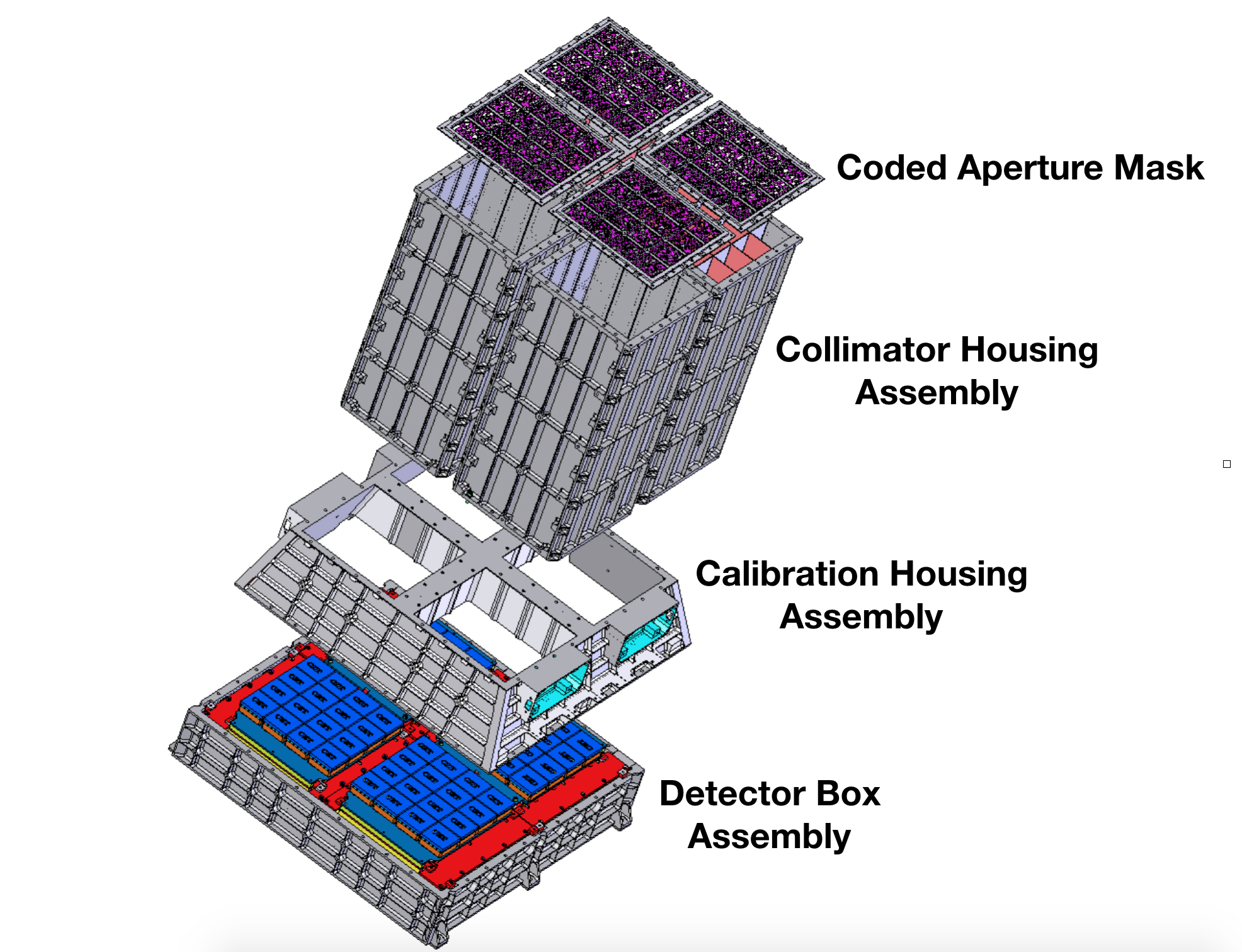
Figure 1: Assembly of the CZTI

CZTI is a ’box-type’ or ’simple’ coded mask telescope where the size of the coded mask and the detector are the same. The full CZTI detector is illuminated only by the on-axis source. Off-axis sources illuminate only a part of the detector depending on the position of the source, this is called “partial coding”. The coded mask for CZTI is designed with seven patterns based on 255-element pseudo-noise Hadamard set Uniformly Redundant Arrays (URA) (Caroli $et~{}al$., 1987). Each pattern has 16$\times$16 mask elements and used as a mask for an individual detector module. A random arrangement of these patterns into a 4 $\times$ 4 array results in the mask pattern for the first quadrant (quadrant A). The coded masks for the other quadrants (B, C, and D) were obtained by rotating the mask pattern of quadrant A by 90$\degree$, 180$\degree$ and 270$\degree$ respectively. Figure 2 shows the mask pattern for all four quadrants of CZTI. In the figure, closed mask elements are represented in black and the open ones in white.

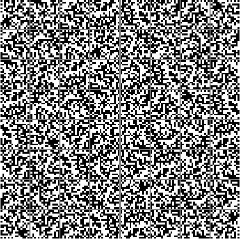
Figure 2: CZTI coded aperture mask for all four quadrants designed using 255 element pseudo-noise Hadamard set Uniformly Redundant Arrays. One extra closed element is added to each URA to obtain a square pattern. Here black areas represent closed mask elements and white areas represent open ones.

CZTI has a total geometric area of 976 cm² achieved using 64 detector modules, divided across four independent quadrants. Each CZT detector module is of size 39.06 mm$\times$39.06 mm$\times$ 5 mm and contains 256 pixels arranged in a 16$\times$16 array. An individual pixel in the array is of size 2.46 mm$\times$2.46 mm, except at edge rows which are 2.31 mm wide. Thus, the edge pixels are of size 2.31 mm$\times$2.46 mm, and the corner pixels are of size 2.31 mm$\times$2.31 mm.

A passive collimator wall of height 400 mm separates any two adjacent modules, restricting the view of each detector module to the coded mask directly above it. The collimator thus restricts the Field of View (FOV) of CZTI to 4.6$\degree$ $\times$ 4.6$\degree$ FWHM at energies below 100 keV. For energies above 100 keV, the collimator walls and the coded mask become progressively transparent, and allows the detection of Gamma-Ray Bursts from all over the sky (Rao $et~{}al$., 2016). Table 1 lists the main characteristics of CZTI. A detailed description of CZTI and its science goals may be found in (Bhalerao $et~{}al$., 2017).

Detector	Cadmium-Zinc-Telluride
Pixels	16384 (64 modules of 256 pixels each)
Pixel size	2.46 mm $\times$ 2.46 mm
Imaging method	Coded Aperture Mask
Field of View	4.6° $\times$ 4.6°
Angular resolution	$\sim$ 8 arc min (18 arc min geometric)
Energy resolution	$\sim$ 8% @ 100 keV
Energy range	20 $-$ 100 keV for collimated FOV (20 $-$ 380 keV for all sky)
Sensitivity	0.5 mCrab (5 sigma; 104 $s$)

Table 1: The important characteristics of CZT Imager.

CZTI records the distribution of counts as a function of position on the detector. The observed count distribution does not correspond to a sky image. The latter is obtained by subjecting the observed pattern to a image reconstruction procedure.

2 Imaging Calibration of CZTI

Like every space astronomy payload, the CZTI flight model underwent a phase of calibration on ground to characterise the pixel behaviour, effective area, imaging and spectral response, etc. The ground-based calibration was carried out by exposing the instrument to various radioactive sources placed at a finite distance from the detector. After launch, the first six months were devoted to carry out in-flight calibration using observations of astronomical sources.

CZTI image reconstruction is a two-step process, the first step is to acquire a spatially coded detector data, and the second step involves reconstruction of the observed image by decoding the collected data. The reconstruction is computationally expensive and performed offline, i.e., on the ground. A variety of image reconstruction algorithms are available, from which a choice is made based on the available computing resources, degree of crowding, nature of the background and the required accuracy. CZTI is a photon-counting detector and records the time of arrival, energy and position on the detector of each detected photon. CZTI image reconstruction starts by creating a two-dimensional map of total counts recorded in each pixel, called a Detector Plane Histogram (DPH). As the detection efficiency varies across the pixels, the DPH is normalized by the relative quantum efficiency (QE) of individual pixels to obtain a Detector Plane Image (DPI). The relative quantum efficiency (QE) of the pixels are available as a part of the CZTI Calibration Database (CALDB). The DPI represents a scaled shadow of the mask on the detector plane cast by the sources in the FOV. The pattern of the DPI depends on the position of the source in FOV and the recorded counts in each pixel depend on the intensities of these sources. If the position or intensity of a source changes, so would the total number of photons recorded by each pixel. The DPI is used as an input to the image reconstruction algorithm. We have used three variants of the Cross-Correlation, namely, mask cross-correlation (Skinner $et~{}al$., 1987; in’t Zand, 1992), shadow cross-correlation, balanced cross-correlation (Fenimore & Cannon, 1978; in’t Zand, 1992) and RichardsonLucy (Richardson, 1972; Bhattacharya, 2006; Shankar & Bhattacharya, 2003) techniques for CZTI imaging calibration.

In this paper we report the results of imaging calibration of CZTI, both on-ground and in-flight, in the sections to follow.

2.1 CZTI On Ground Calibration

We performed CZTI ground calibration in two phases, in the first phase, the coded mask and the imaging procedure were validated, and in the second phase, we calibrated the fully assembled CZTI to validate the imaging response.

2.1.1 On Ground Calibration using the Qualification Model

One detector module with 16$\times$16 pixels of a Qualification Model (QM) was used first to verify the imaging procedure. A fixture, schematically shown in figure 3, was made to perform the ground calibration. In the fixture, the source and the mask plate were placed at the height of $897.5~{}mm$ and $484~{}mm$ respectively above the detector. Two radioactive sources, Americium-241 (with a line at 59.54 keV) and Cobalt-57 (with lines at 122 keV and 136 keV) were used to validate the coded mask and the imaging procedure. ²⁴¹Am had count rate of 400 counts/sec and ⁵⁷Co had 350 counts/sec. We selected several locations on the fixture, including the centre as well as a few offset locations and carried out multiple observations at these locations. The finite distance of the source from the detector causes the shadow to differ from what would be expected from a distant astronomical source. In the laboratory setup built for CZTI ground calibration, one mask element cast its shadow over 2$\times$2 detector pixels. Hence, only a quarter of the mask illuminated the entire detector module, despite the mask and the detector being of the same physical size. For image reconstruction, we computed a library of the expected shadows of the mask on the detector, spanning source positions over $\pm 19.5$ mm from the centre in both X and Y directions, in steps of $0.25$ mm.

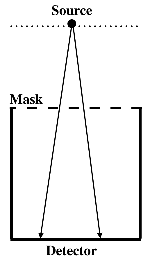
Figure 3: A schematic representation of the assembly made to test the coded mask imaging procedure using CZTI Qualification Module. In this setup the source was placed 897.5 mm above the detector while the mask is located at a height of 484 mm above the detector.

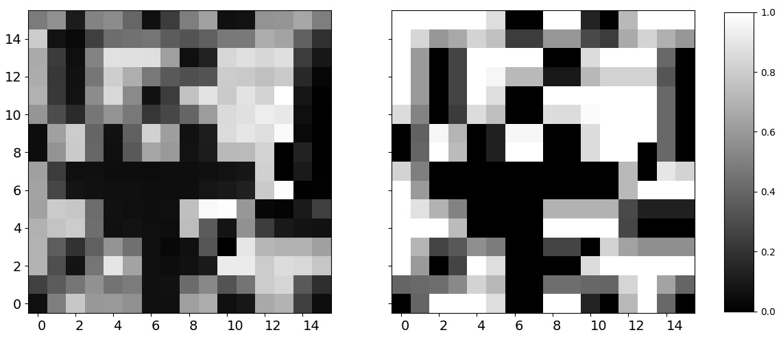
Figure 4: The expected (left panel) and observed (right panel) shadow of the mask on the detector when the radioactive source ²⁴¹Am was placed directly above the centre of the detector, in the arrangement shown in Fig. 3. The observed pattern is normalized and dead/noisy pixels are ignored.

We obtained five different data sets by placing the ²⁴¹Am source at different locations, including the centre and a few offset positions. One data set was also obtained by simultaneously placing two sources, ²⁴¹Am and ⁵⁷Co at two different locations on the fixture. In figure 4, the left panel shows the expected shadow pattern, and the right panel shows the observed pattern when the source was placed on a normal passing through the centre of the detector. The CZTI electronics recorded the pixel ID, energy and time of each detected photon, creating an event list. The DPH were constructed by binning the events as a function of pixel number and along with the computed shadow library were used as input to the imaging procedure. For image reconstruction during the ground calibration, we used Richardson-Lucy and cross-correlation algorithms.

Figure 5 shows the reconstructed image when ²⁴¹Am source was placed at the center using Richardson-Lucy and cross-correlation methods, and image profiles of X and Y cross sections of the reconstructed image is shown in figure 6. Figure 7 shows the reconstructed image using cross-correlation for the simultaneous observation of two sources where ²⁴¹Am source was placed at the offset of -10.25$~{}mm$ and ⁵⁷Co was placed at the offset of -10.25$~{}mm$ from the center in X-direction.

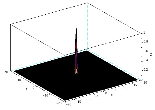
(a) Reconstructed image using Richardson-Lucy

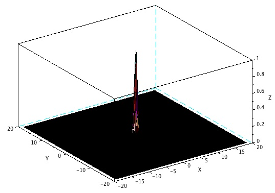
(b) Reconstructed image using cross-correlation

Figure 5: Reconstructed image using Richardson-Lucy and cross-correlation methods, when source is at the centre of the detector.

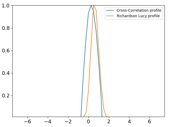
(a) Image profile in X cross sections.

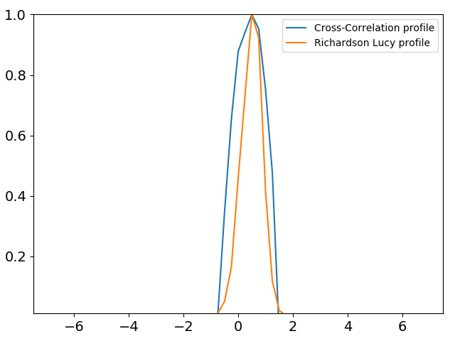
(b) Image profile in Y cross section.

Figure 6: Image profiles of X and Y cross sections of the image reconstructed using Cross-Correlation and Richardson-Lucy algorithm.

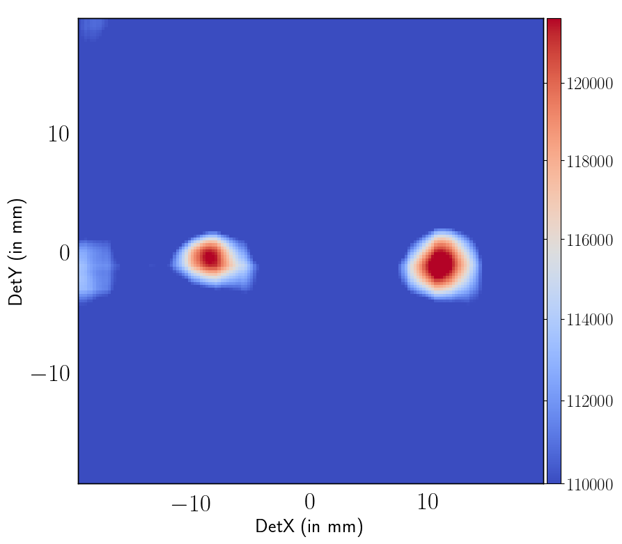
Figure 7: Reconstructed image using cross-correlation method for the simultaneous observation of two sources where ²⁴¹Am source was placed at the offset of -10.25$~{}mm$ and ⁵⁷Co was placed at the offset of +10.25$~{}mm$ from the center in X-direction. Sources were of almost equal strength.

We then compared the reconstructed source location from the image with the source position set in the lab during the acquisition of the data. Table 2 presents the results of this exercise.

Lab location (in mm)	CC (in mm)	RL (in mm)
(0.0,0.0)	(0.7,0.75)	(0.5,0.4)
(0.0,-10.25)	(0.2,-9.75)	(0.25,-9.7)
(0.0,10.25)	(0.5,11.0)	(0.5,11.0)
(-10.25,0.0)	(-9.85,0.5)	(-9.75,0.25)
(10.25,0.0)	(11.0,0.5)	(10.65,0.35)

Table 2: Position of source in lab and reconstructed positions using cross-correlation and Richardson-Lucy algorithm.

In the case of two-source observation, we constructed two separate DPHs, one from photons recorded near $60$ keV, and another from photons near $122$ keV. Table 3 summarises the reconstruction result for the observation with two sources.

Source	Lab location (in mm)	CC (in mm)	RL (in mm)
${}^{241}Am$	(-10.25,0.0)	(-9.0,0.0)	(-9.0,-0.2)
${}^{57}Co$	(10.25,0.0)	(10.7,-1.0)	(10.5,-1.25)

Table 3: Lab position of the source during the observation and reconstructed source position using Cross-correlation and Richardson-Lucy algorithm.

The results from cross-correlation and Richardson-Lucy methods agreed within 0.5 mm. The source positions set in the lab and the reconstructed positions were consistent well within 1 mm, except for one case where the deviation was 1.25 mm. This discrepancy in the reconstructed position could be due to the inaccuracy in the manual placement of the radioactive source. The location accuracy of 1.0 mm at a source height of 897.5 mm corresponds to an angular accuracy of 3.8 arcmin. In all the above reconstructions, the total number of source photons used are more than a million and average background count was 350 counts/sec. To examine the reliability of the algorithm, image reconstruction was also performed with a smaller subset of photons. Event lists containing $10^{5}$, $10^{4}$, $10^{3}$ and $10^{2}$ photons were selected randomly from the full event list and imaging was performed using them. We repeated the imaging procedure with ten different random event sets in each case to estimate the variation in reconstruction results due to counting statistics. Table 4 lists the absolute difference (in mm) between the source location reconstructed using the subset event list and the full event list.

Trial No	$10^{5}photons$	$10^{4}photons$	$10^{3}photons$	$10^{2}photons$
1	0.0	0.0	0.0	0.55
2	0.0	0.25	2.70	0.55
3	0.0	0.25	0.35	0.55
4	0.0	0.0	0.0	1.03
5	0.0	2.85	0.0	0.25
6	0.0	2.85	0.25	0.75
7	0.0	0.0	0.25	0.50
8	0.0	0.25	0.25	0.79
9	0.0	0.0	0.25	0.25
10	0.0	0.0	0.35	0.25

Table 4: Absolute difference (in mm) between the source location using a smaller number of events and the full event list.

The results show that the reconstruction is quite robust, and the RMS deviation is within 1.3 mm (5 arcmin).

2.1.2 On Ground Calibration using the Flight Module

The results from the qualification model confirmed the working of the coded mask and the imaging procedure. The four quadrants of the CZTI Flight Model (FM) were then assembled and calibrated.

The ground calibration of the FM was carried out by shining three different radioactive sources on individual quadrants. In addition to ²⁴¹Am and ⁵⁷Co, a ¹⁰⁹Cd source with lines at 22 keV and 88 keV was used. Figure 8 shows the laboratory setup used for the FM calibration. The perpendicularity of placement of the source with respect to the detector was ensured using a laser beam and a mirror.

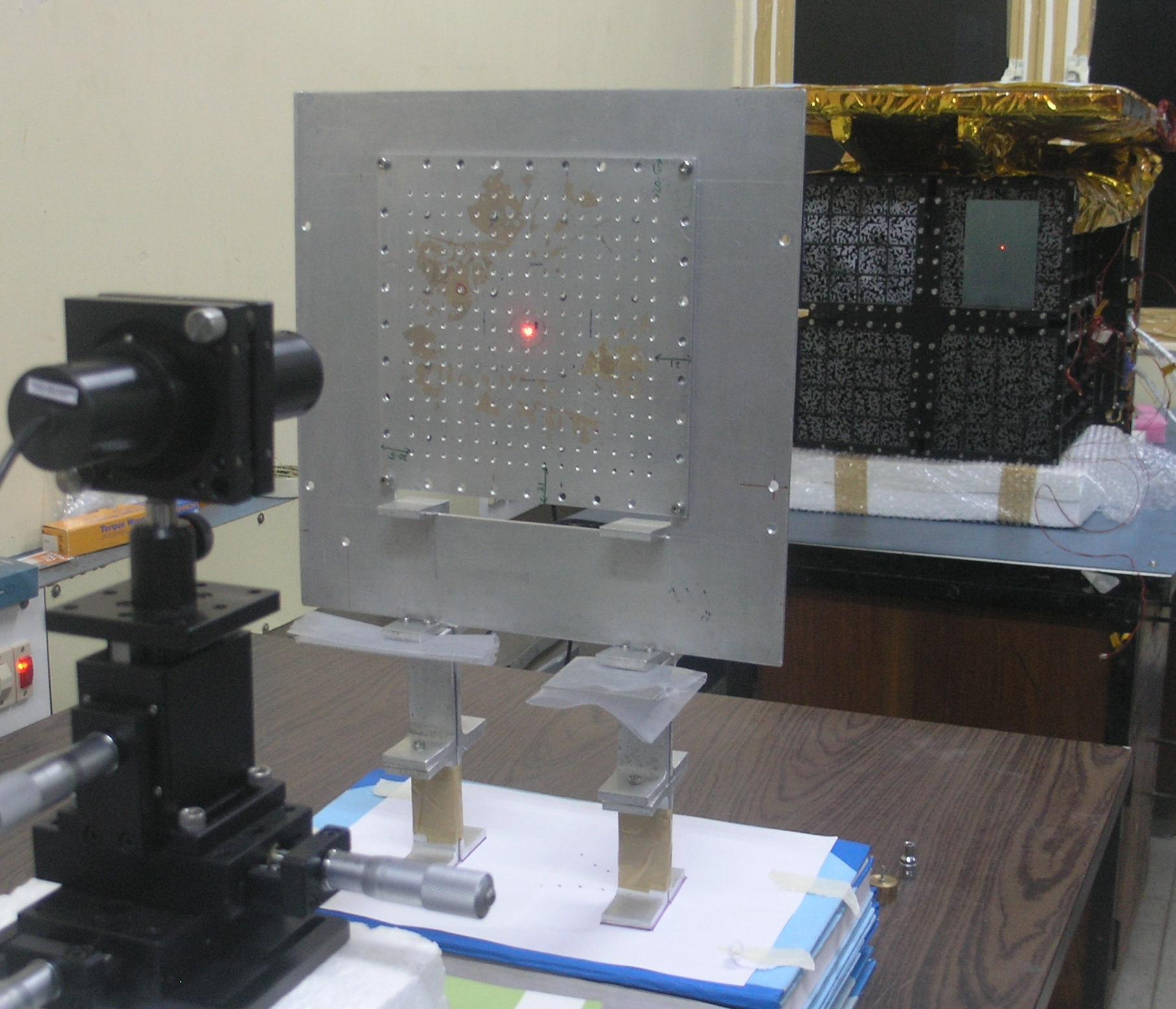
Figure 8: Laboratory setup at Tata Institute of Fundamental Research (TIFR) used for the CZTI FM calibration

The radioactive source was positioned at different locations on the quadrant using the fixture. Five reference positions P1, P2, P3, P4, and P5, directly above the intersection of four adjacent detector modules, were selected to place the source. Figure 9 shows the five selected positions.

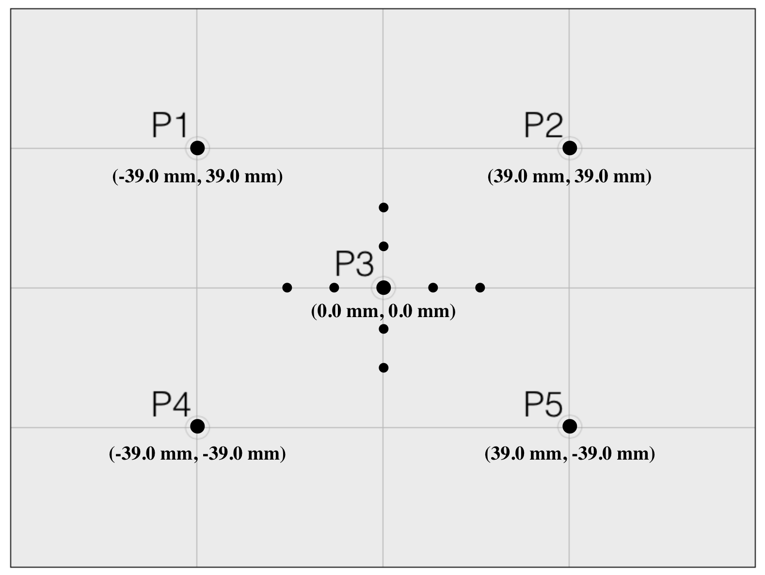
Figure 9: Reference positions on the fixture for a quadrant

In addition to the five reference positions, the radioactive source was also placed at a few locations, shifted in the X and Y directions from the central reference P3, as shown in Fig. 9. The height of the source plane was 2 metres above the detector. The uncertainty in the horizontal and vertical positioning of the source is estimated to be $\sim 2.5$ mm and $\sim 1$ cm respectively. The source illumination axis was kept perpendicular to the detector within an accuracy of about 0.14$\degree$. A library of shadows was created by computing expected shadow patterns for a range of source positions, spanning 39 mm on either side of each reference position in both directions in steps of 0.25 mm. The acquired datasets were then analyzed using cross-correlation and Richardson-Lucy algorithms. Figure 10 shows the reconstructed source profile using the Richardson-Lucy algorithm for an observation where the radioactive source is located at position P3.

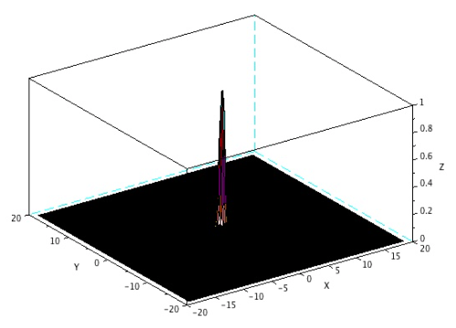
Figure 10: Reconstructed source profile using the Richardson-Lucy method when the source is placed at the central reference P3 during FM ground calibration.

Table 5 shows the deviation, in mm, of the reconstructed locations of the sources from the expected ones. In the flight model calibration, the source was at the height of 2000 $mm$, whereas during the qualification model calibration source was at 897 $mm$ above the detector. Hence, in the flight model calibration, we see more deviation than the deviation seen the qualification model calibration.

Sr.No.	Quadrant ID	Lab Location	Source	CC (in mm)	RL (in mm)
1	0	P1	Am	(3.00, 3.00)	(2.50, 1.50)
2	0	P3	Am	(3.00, 2.25)	(2.75, 2.00)
3	0	P4	Am	(-0.25, 1.75)	(-0.50, 1.75)
4	0	P5	Am	(-2.00, 4.00)	(-2.00, 4.00)
5	0	P3	Co	(-2.00, 2.00)	(-1.75, 1.50)
6	0	P3+(-10,0)	Co	(0.50, 2.00)	(-0.50, 1.50)
7	0	P3+(-20,0)	Co	(0.00, 2.25)	(-0.50, 2.00)
8	0	P3+(10,0)	Co	(0.75, 2.00)	(0.75, 2.00)
9	0	P3+(20,0)	Co	(1.25, 2.25)	(1.00, 2.00)
10	0	P3+(0,10)	Co	(0.50, 1.00)	(0.50, 1.00)
11	0	P3+(0,20)	Co	(2.00, -1.75)	(1.00, -1.75)
12	0	P3+(0,-10)	Co	(2.00, -3.00)	(0.00, -3.75)
13	0	P3+(0,-20)	Co	(-1.25, -2.75)	(-2.00,- 2.75)
14	0	P2	Co	(-1.25, -2.00)	(-1.25, -1.75)
15	0	P4	Co	(-3.00, 1.75)	(-2.50, 1.75)
16	0	P5	Co	(-2.25,1.50)	(1.25 ,1.75)
17	1	P3	Co	(0.25,-0.50)	(0.50, -0.25)
18	1	P3+(-10,0)	Co	(0.50, 1.25)	(0.00, 1.00)
19	1	P3+(10,0)	Co	(0.00, 0.50)	(0.25, 0.50)
20	1	P3+(0,10)	Co	(0.25,0.25)	(0.25, 0.0)
21	1	P3+(0,20)	Co	(0.75,-0.50)	(0.50,-0.25)
22	1	P3+(0,-10)	Co	(0.00,-1.25)	(0.25, -1.00)
23	1	P3+(0,-20)	Co	(1.0, -1.00)	(0.75, -1.25)
24	2	P3	Co	(1.25, 0.75)	(2.25, 0.75)
25	2	P3+(-10,0)	Co	(1.00, 0.75)	(0.75, 0.75)
26	2	P3+(-20,0)	Co	(1.00, 1.00)	(0.00, 1.25)
27	3	P1	Am	(-0.75, 3.00)	(-1.25, 1.00)
28	3	P2	Am	(3.00, 2.25)	(3.25, 2.25)
29	3	P3	Am	(0.75, 0.75)	(0.75, 0.75)
30	3	P4	Am	(2.25, 1.25)	(2.50, 1.00)
31	3	P3	Co	(0.00, 1.25)	(1.25, 1.00)
32	3	P3+(-10,0)	Co	(-1.00, 0.00)	(-1.00, 0.00)
33	3	P3+(-20,0)	Co	(-0.50, 0.00)	(-1.50, 0.25)
34	3	P3+(10,0)	Co	(0.75, 0.00)	(1.00, 0.75)
35	3	P3+(20,0)	Co	(1.00, 0.00)	(1.75, 1.25)
36	3	P3+(0,10)	Co	(0.25, -0.75)	(0.25, -0.75)
37	3	P3+(0,20)	Co	(1.50, -0.50)	(1.50,0.50)
38	3	P3+(0,-10)	Co	(0.25, -1.00)	(0.25, -1.00)
39	3	P3+(0,-20)	Co	(1.25, -2.00)	(1.00, -2.00)
40	3	P1	Co	(-1.00, 2.00)	(-2.00, -0.50)
41	3	P2	Co	(2.25, 2.25)	(0.00, 2.25)
42	3	P4	Co	(0.00, 0.00)	(0.00, 0.00)
43	3	P5	Co	(1.00, 0.75)	(1.00, 0.75)

Table 5: Laboratory source positions set during FM ground calibration and the offsets in reconstructed source positions by Cross-correlation and Richardson-Lucy algorithms. Units are millimetres.

Figure 11 shows a scatter plot of deviations in the reconstructed locations from those expected. In most cases, the deviation is well within 1.5 mm except for a small fraction extending up to 3 mm. The deviation of 3 mm at a height of $2000~{}mm$ corresponds to an angular deviation of 5 arcmin, within the design goal of 8 arcmin for the CZTI.

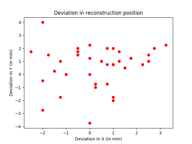
Figure 11: Deviation of the source positions recovered using the Richardson-Lucy algorithm with respect to the expected values during the FM ground calibration.

2.2 In-flight Calibration

The first six months after the launch of AstroSat was reserved for the Performance Verification (PV) and calibration of all the instruments. During this period, several calibration observations were conducted of the Crab nebula, one of which, observation ID 20160331_T01_112T01_9000000406, was used to characterise the post-launch imaging performance. This observation was performed from UT 2016-03-31 05:39:19 to 2016-04-03 03:55:11, adding up to a total of 114 ks exposure time. The observed data was analyzed using the CZTI data analysis pipeline. Figure 12 shows the reconstructed sky image of the Crab from all four quadrants of CZTI using the mask cross-correlation technique. In the images, the expected location (shown as a yellow circle) of the source matches the peak of the reconstructed profile for quadrants A and B, while images from quadrants C and D show a deviation of 0.29$\degree$ in the Y direction. For quadrant B, although the reconstructed source location is correct, there is an extended tail in the X-direction.

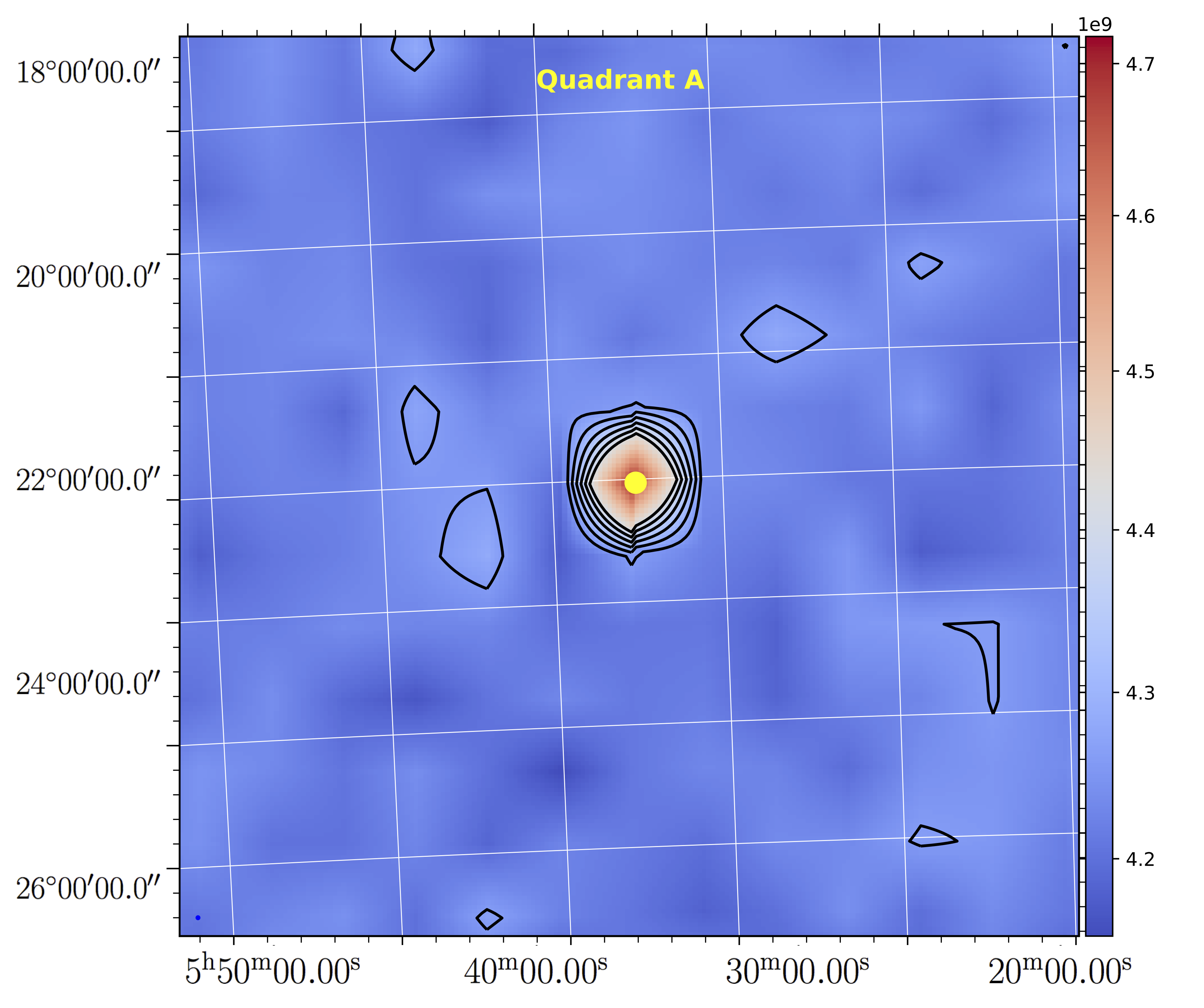
(a) Quadrant A.

(b) Quadrant B.

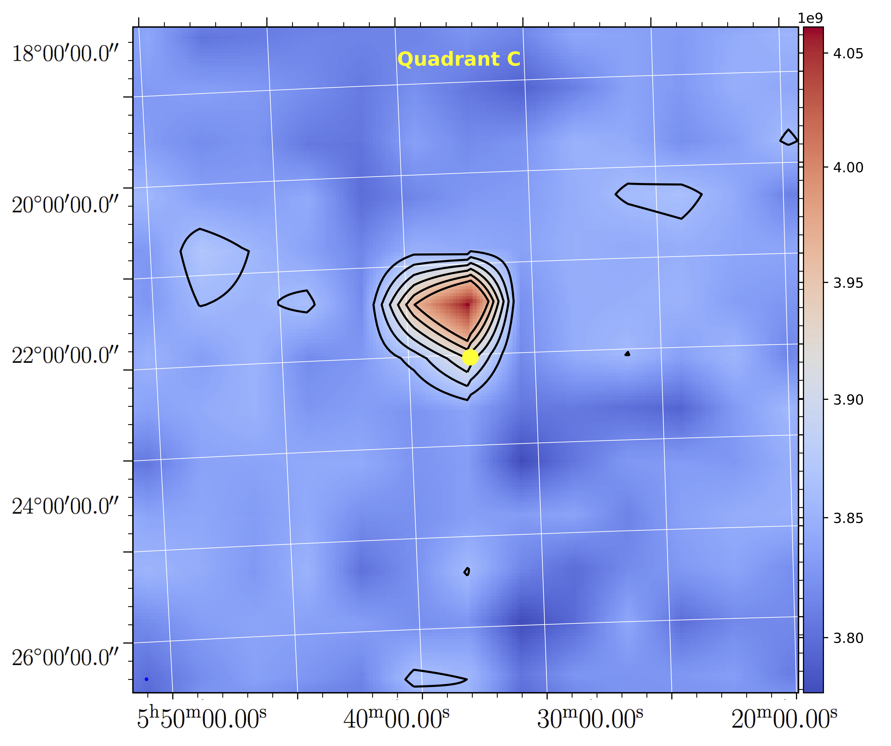
(c) Quadrant C.

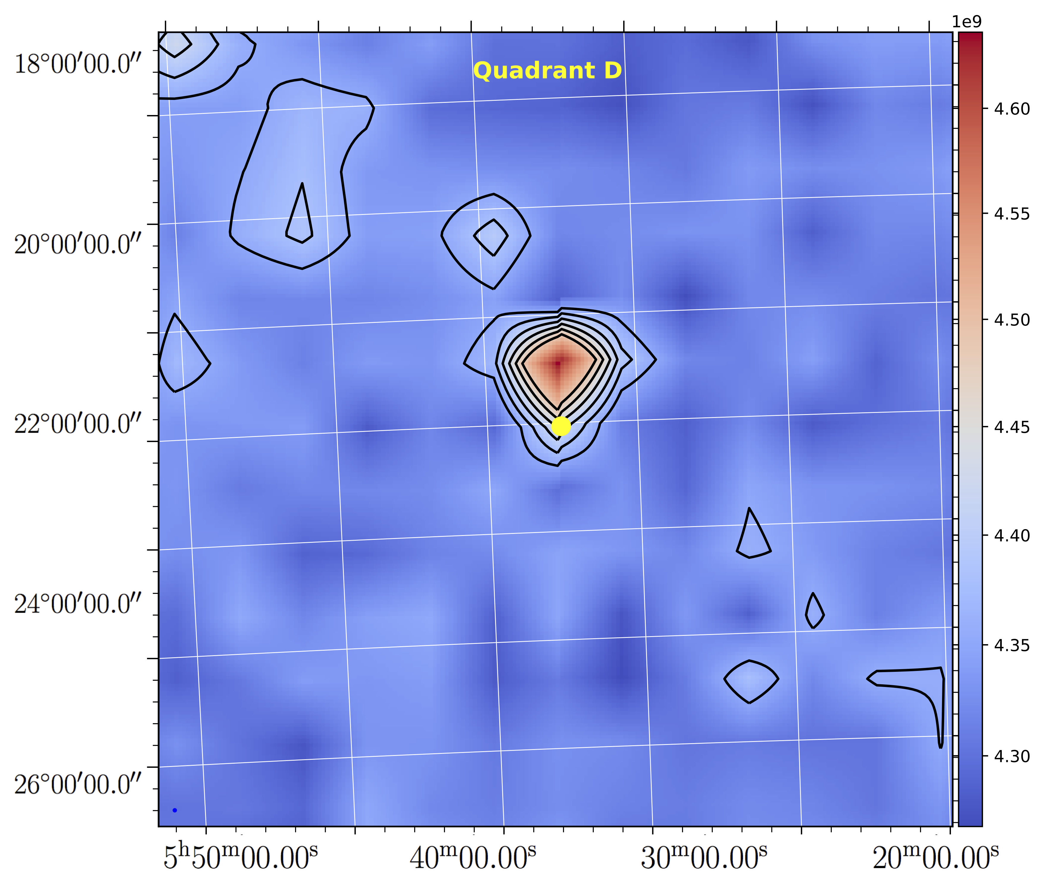
(d) Quadrant D.

Figure 12: Image of the Crab Nebula reconstructed from CZTI data using mask cross-correlation technique for observation id 9000000406. Note that the angular extent of the source is well within the resolution of the CZTI, so the image profile primarily reflects the angular response of CZTI.

To understand the discrepancy between the expected and the reconstructed images, various experiments and simulations were performed. For quadrant A, the reconstruction was as expected, so the experiment started with quadrant B, which showed an extended peak. The following possible scenarios were investigated to understand the cause of the extension and the shifts observed in the reconstructed image.

1. Extension or shift because of measurement error in the distance between the detector and the mask

2. Extension or shift because of unstable pointing

3. Extension or shift because of module dependency

4. Extension or shift because of misalignment between the detector and mask

2.2.1 Extension or shift because of measurement error in the distance between the detector and the mask

The distance between the coded aperture and the detector is a key factor in the design of a coded mask instrument. A wrong value for this used in the reconstruction process could lead to distortions in the recovered image. In the case of CZTI, the mask plate is placed 481 mm above the detector as per design. To investigate the effects of a possible error in this value, we simulated DPIs with the mask placed at heights 470 mm, 460 mm, 450 mm and 400 mm above the detector, and subjected them to the same image reconstruction as employed for the real data. This is a much exaggerated range of heights than the error margin that could be expected in reality. Figure 13 shows the images reconstructed from simulated DPI with the mask plate placed at 450 mm and 400 mm respectively. The reconstructed images show neither an extension nor a shift. Hence, an error in mask height was ruled out as a possible cause of the image distortions observed.

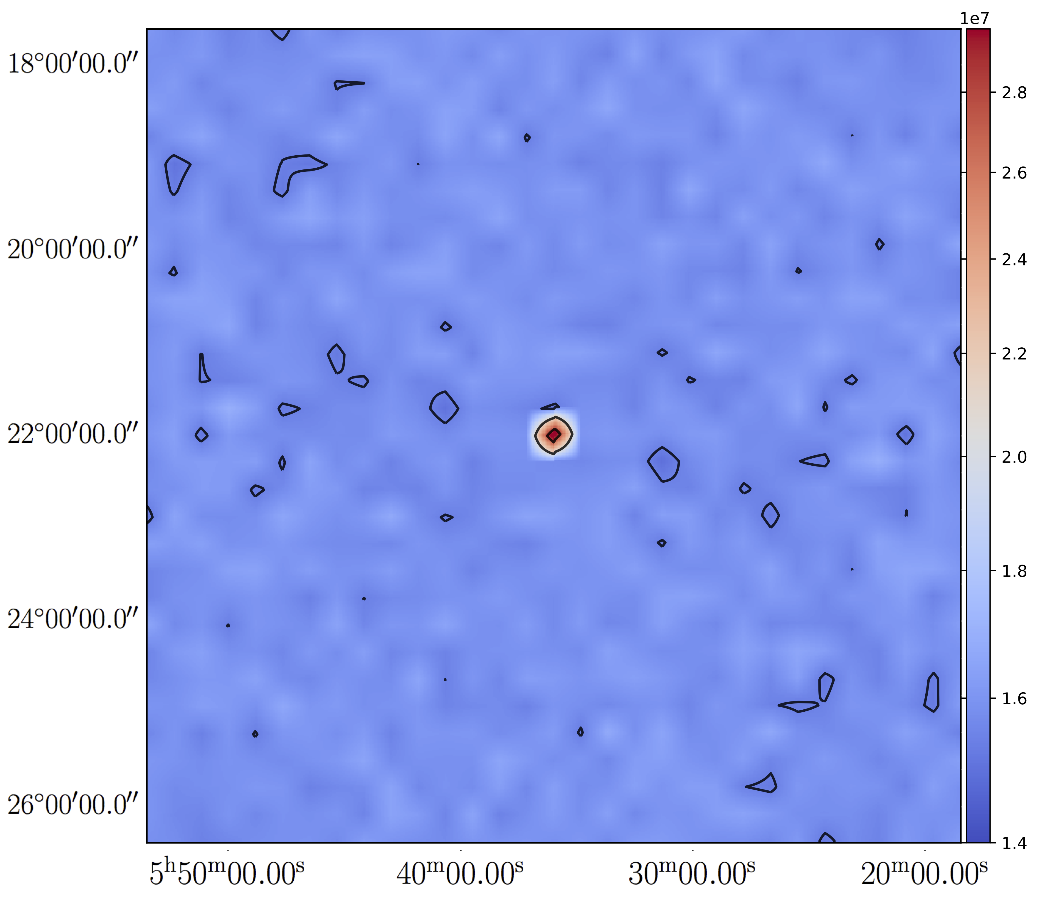
(a) Mask plate height $400~{}mm$ from detector.

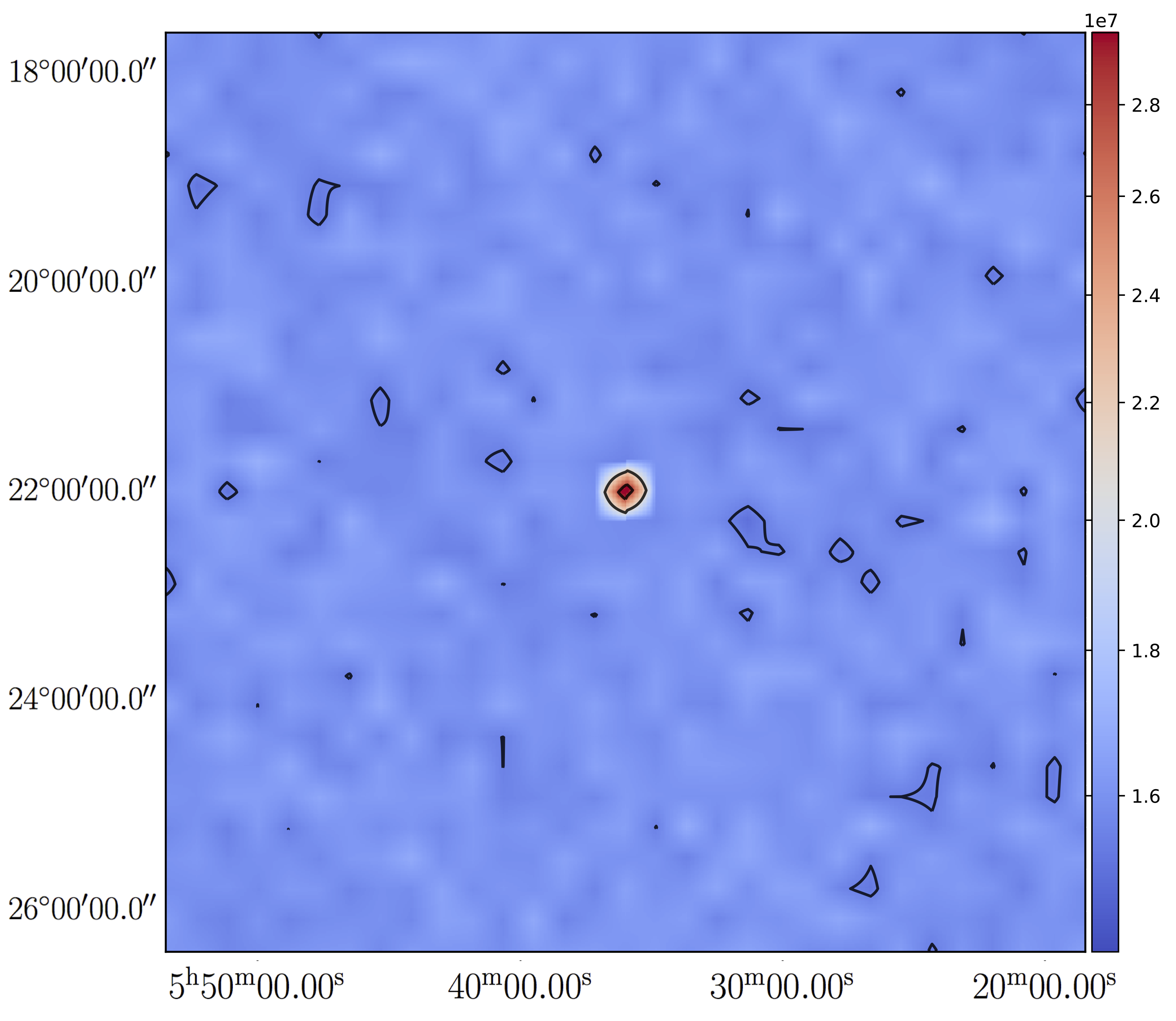
(b) Mask plate height $450~{}mm$ from detector.

Figure 13: Image reconstructed from simulated DPI with mask plate placed at a height $400~{}mm$ (Left panel) and $450~{}mm$ (Right panel)

2.2.2 Extension or shift because of planar misalignment between the mask and detector

The image reconstruction depends strongly on the planar alignment between the coded aperture and the detector, including any offset and rotations. If the mask and the detector are misaligned, then it can affect the reconstructed image. To examine the effect of a possible planar misalignment between the mask and detector, we simulated DPIs with planar misalignment of 1$\degree$, 3$\degree$, 5$\degree$,10$\degree$ and reduced these DPIs using the image reconstruction method. Figure 14 shows the images reconstructed from simulated DPI with the mask plate tilted with 5$\degree$,10$\degree$. The reconstructed images show neither an extension nor a shift. Hence, we discarded the possibility of planar misalignment between the mask and the detector as the reason behind the image distortions observed.

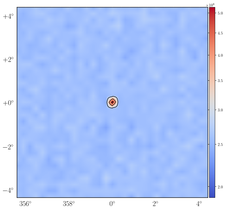
(a) Mask plate tilted with 5 degree from the detector plane.

(b) Mask plate tilted with 10 degree from the detector plane.

Figure 14: Reconstructed images by introducing planar misalignment between the mask and detector.

2.2.3 Extension or shift because of unstable pointing

If the time span over which the data for the DPI ere accumulated saw a significant variation in the pointing of the CZTI, then the reconstructed image could show a smearing. Individual Crab images can be constructed from the CZTI data for integration times as short as 30 sec. Doing so with quadrant B data showed very similar extension in individual images (Figure 15). Examination of the satellite attitude data, collected at 128 ms sampling, revealed that the attitude jitter was no more than 0.045 degree rms over the time scale of minutes to hours, thus making it very unlikely that the observed image extension could result from it.

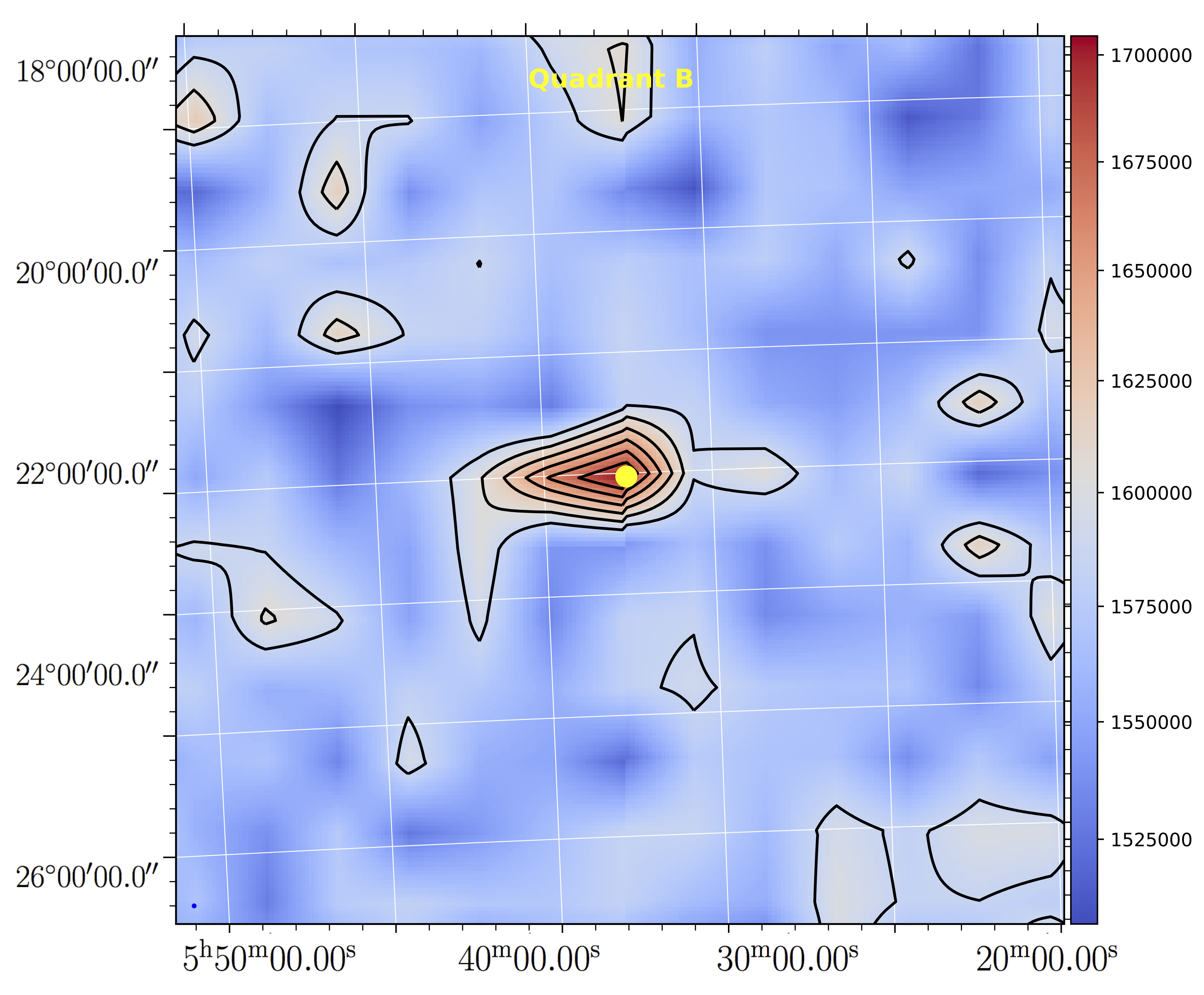
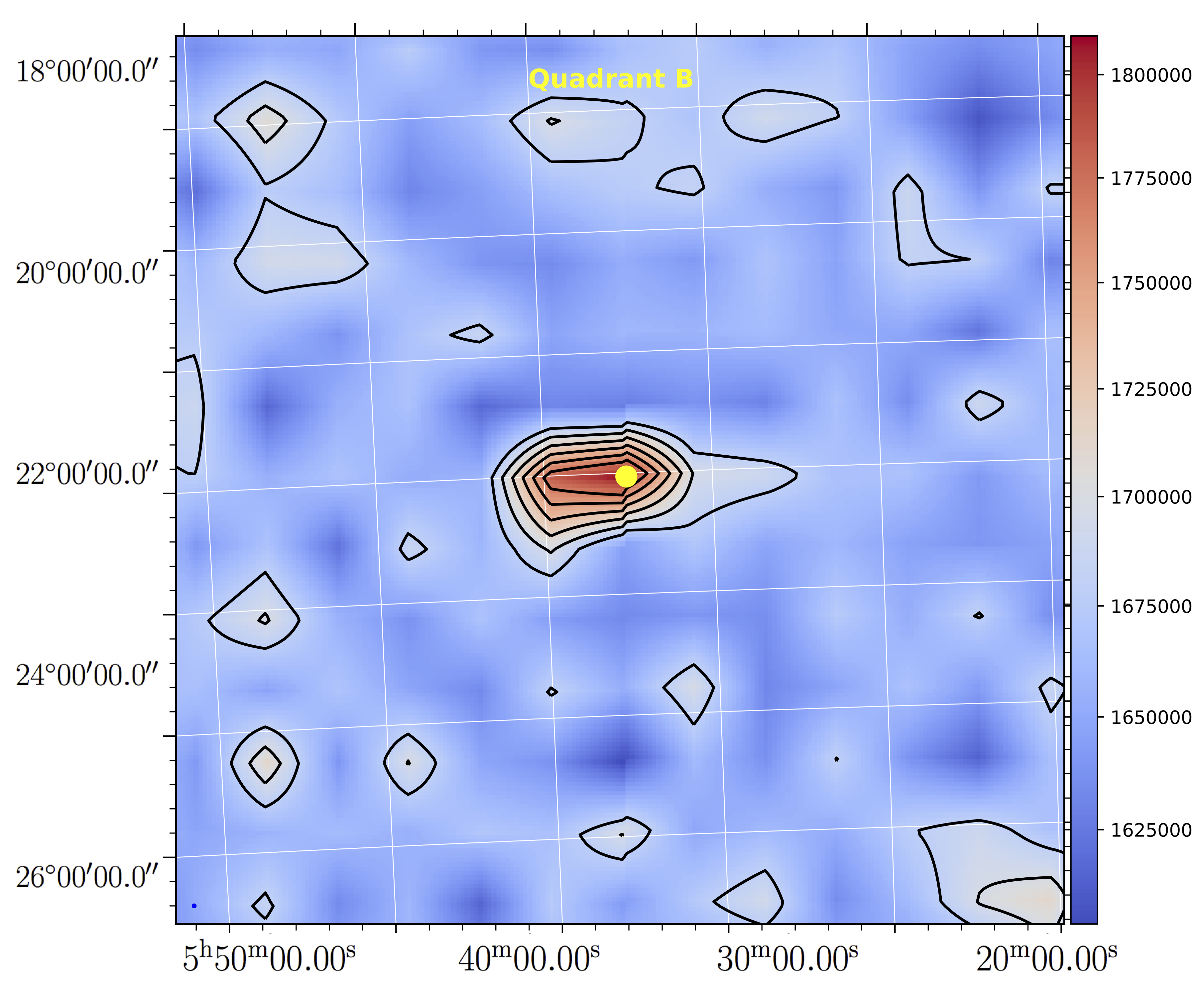
Figure 15: Reconstructed image at two time bins for Quadrant B

2.2.4 Module dependence

Each CZTI quadrant is composed of 16 detector modules, all of which operate independently. At this point it was essential to establish whether the image distortion observed was a quadrant level phenomenon or do individual detector modules in a quadrant display discordant behaviour. We therefore reconstructed images using events from individual modules in all four quadrants. In the reconstructed images, no module in the quadrant A showed any shift or extension. However, in quadrant B, 14 modules showed extension and in quadrants C and D, 14 and 12 modules respectively showed the shift in the reconstructed source position. An account of this is presented schematically in Figure 16. This collective display strongly indicated that the image extension or shift was associated with the imperfection of the complete assembly at the level of quadrants.

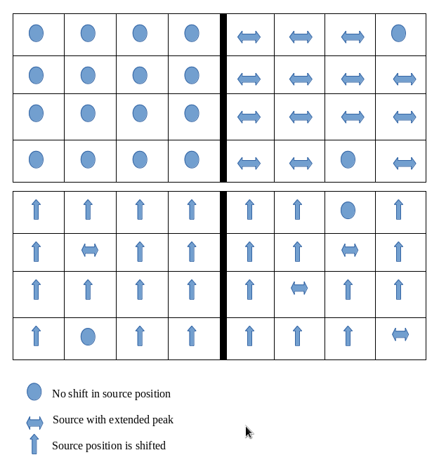
Figure 16: Distortions observed in module level imaging

2.2.5 Detector-mask misalignment

Results from module-level imaging lead us to the possibility of misalignment between the detector and the mask. We performed various simulations to examine the effect of misalignment on the reconstructed images. Initially, we simulated a DPI by shifting the mask pattern by $0.5~{}mm$ in the negative X direction. The source image reconstructed from the simulated DPI showed an extended peak. Next, we shifted the mask pattern at steps of $0.1$ mm in the negative X-direction and compared the simulated image profiles with the observed image profile.

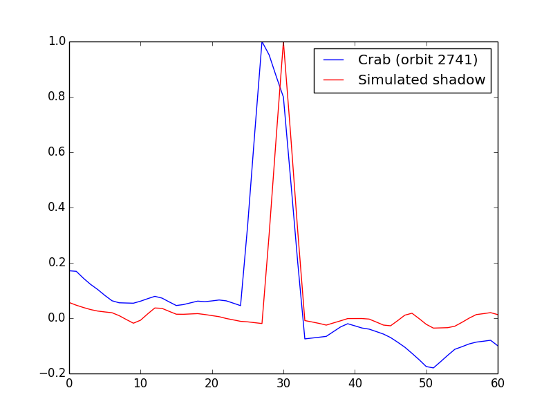
(a) Without mask shift

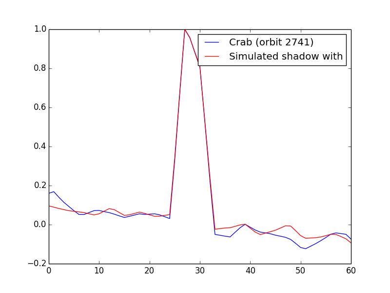
(b) With mask shift

Figure 17: Simulated 1-d image profiles with zero (left panel) and $-0.5$ mm (right panel) shift of the mask pattern in the x-direction, compared with that obtained from observed data

The one-dimensional image profile of the image reconstructed from observed data, and simulated data without any mask shift showed a strong disagreement. However, the image profile of the image reconstructed from simulated data with a mask shift of $-1.45$ mm showed a strong agreement with the observed image profile. Figure 17 shows the one-dimensional image profiles for observed and simulated data generated from the direct cross-correlation image. Then, we simulated DPIs for shifts in the X-direction, from $-1.20$ mm to $-1.65$ mm with a step of $0.05$ mm and compared the resulting images with that observed. The minimum chi-square was found for a mask shift of $-1.45$ mm, figure 19 . Hence, this experiment confirmed that in quadrant B there is a slight misalignment of $-1.45$ mm between the detector and the mask plate in the X-direction. Shifts for other quadrants were also estimated using a similar methodology. Table 6 below outlines the shift in the mask pattern with respect to the detector for all four quadrants.

We have not observed any extension in the reconstructed images during the on-ground calibration. To review the effect of the mask shift on the reconstructed images in near field imaging, we have simulated DPIs for diverging beam radiations shined by a radioactive source under the circumstances similar to the ground calibration. We then subjected the simulated DPIs to the image reconstruction algorithm. Figure  18 shows the reconstructed image generated using the simulated DPH with the mask shift of -1.45$~{}mm$. The reconstructed images did not show any extension or shift in the source position. In near field imaging, one mask element illuminates more than one detector pixel due to the diverging beam of radiations and possible that the mask shift may not affect the reconstructed image.

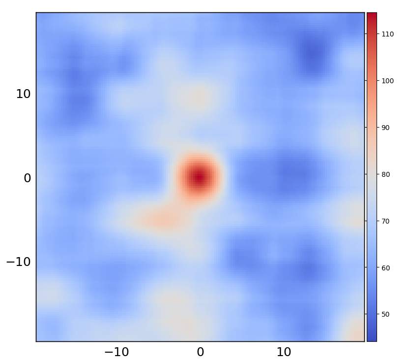
Figure 18: The image reconstructed from simulated DPI with the shifted mask in near field imaging similar to CZTI ground calibration.

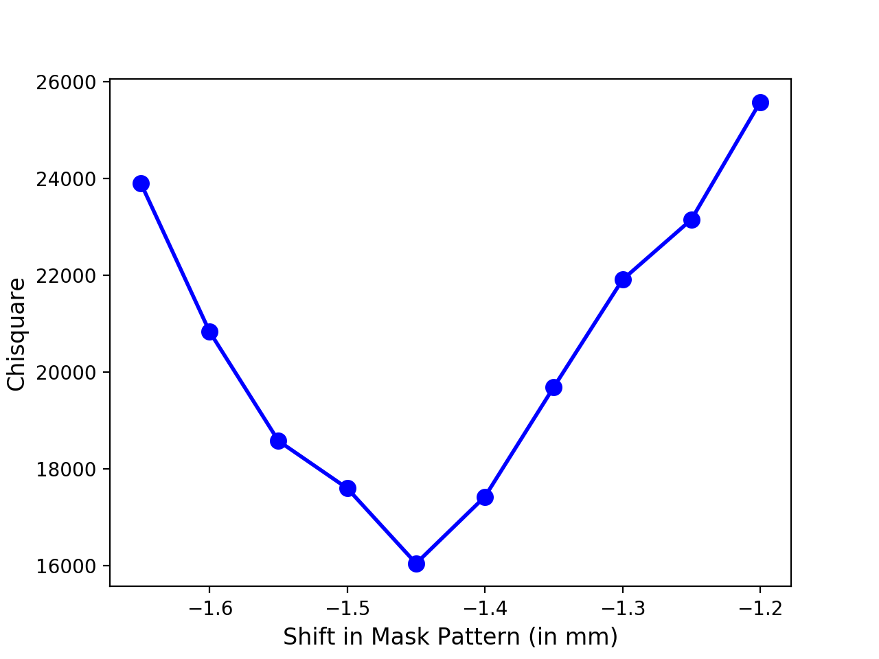
Figure 19: Chi-square value as a function of mask shift in the X direction for Quadrant B.

Quadrant	X shift (in mm)	Y shift (in mm)
A	0.00	0.00
B	-1.45	0.00
C	0.00	1.68
D	0.00	1.50

Table 6: The shift in the mask pattern with respect to the detector for all quadrants.

After calculating the shifts for all quadrants, we corrected for shifts in the imaging algorithm. The section below describes the corrections applied.

3 Correcting for Mask Shifts

In mask cross-correlation, the DPI is cross-correlated with the coded aperture mask. To correct for the shift in the reconstructed image, we multiply a phase matrix in the Fourier domain, as shown in Equation 1.

$$\mathcal{F}^{-1}(\mathcal{F}(DPI)X\mathcal{F}(MASK)*P)$$ (1)

Here, $\mathcal{F}$ is FFT, $\mathcal{F}^{-1}$ is inverse FFT, and P is a phase matrix as described in equation 2,

$$P=e^{i2\pi(f_{x}\delta_{x}+f_{y}\delta_{y})}$$ (2)

Here,
$\delta_{x}$ is the shift in X direction in pixel unit
$\delta_{y}$ is the shift in Y direction in pixel unit
$N_{x}$= number of pixels in X direction
$N_{y}$= number of pixels in Y direction
$f_{x}$= $\frac{-1}{N_{x}}+....+\frac{1}{N_{x}}$
$f_{y}$= $\frac{-1}{N_{y}}+....+\frac{1}{N_{y}}$

(a) Quadrant A.

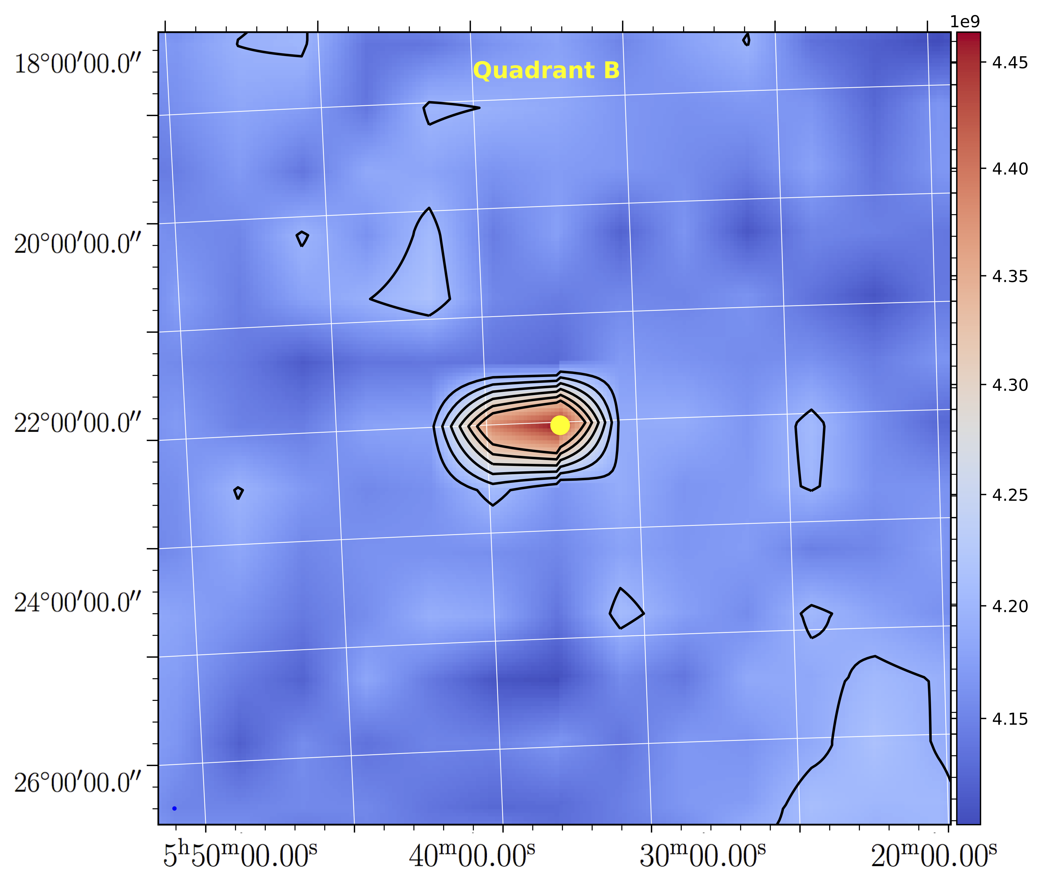
(b) Quadrant B.

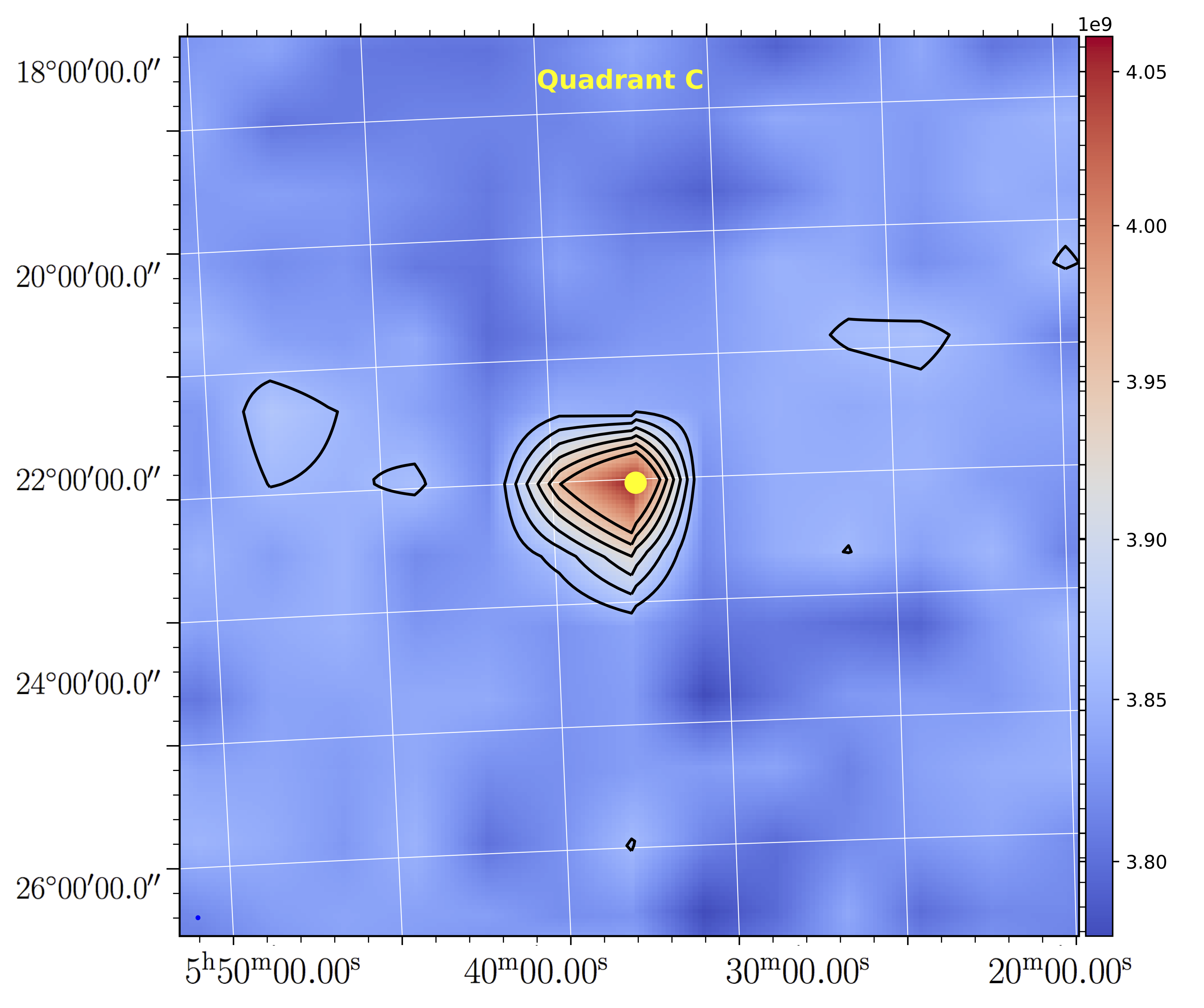
(c) Quadrant C.

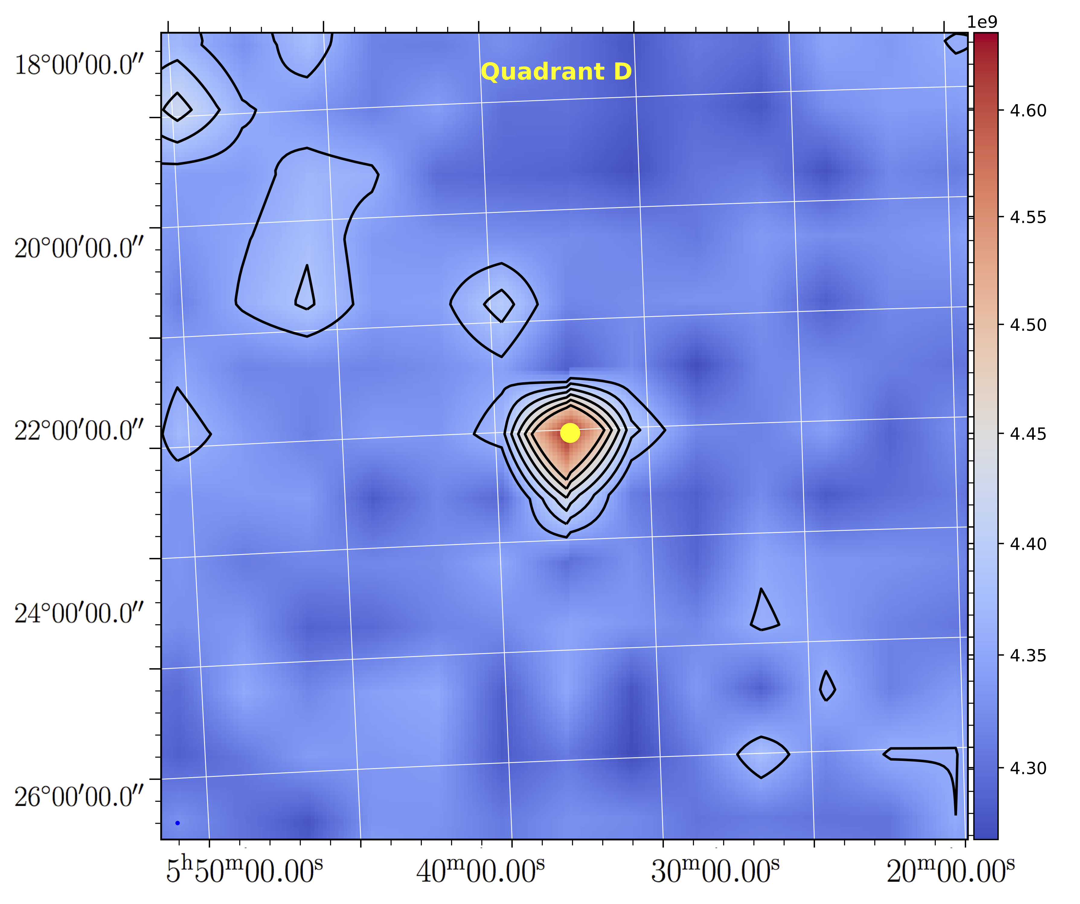
(d) Quadrant D.

Figure 20: Crab nebula image reconstructed using FFT after application of the phase matrix for observation id 9000000406.

After multiplication with the phase matrix and performing inverse FFT, the source is found to be at the expected location. CZTI data analysis pipeline is modified to incorporate the phase shift multiplication to correct the images reconstructed using mask cross-correlation images. Figure 20 shows the reconstructed sky images generated using modified mask cross-correlation for four quadrants. The phase matrix multiplication compensated for the shift in the reconstructed image, but the extension in quadrant B was not corrected. The extension in the image can be corrected using the shadow cross-correlation method (section LABEL:shadowcrosscorrelation) using computed shadows that incorporate the measured mask shifts.

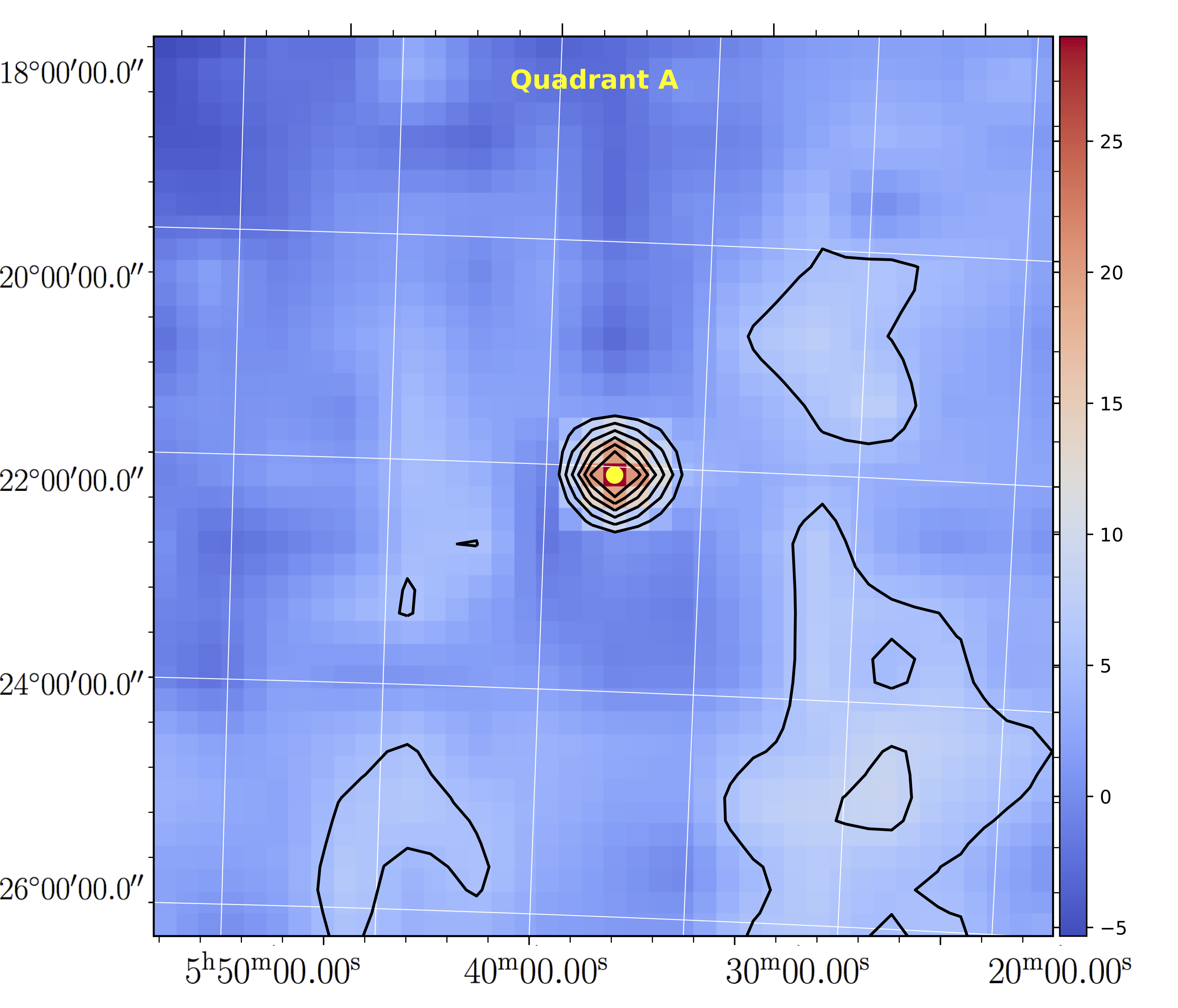
(a) Quadrant A.

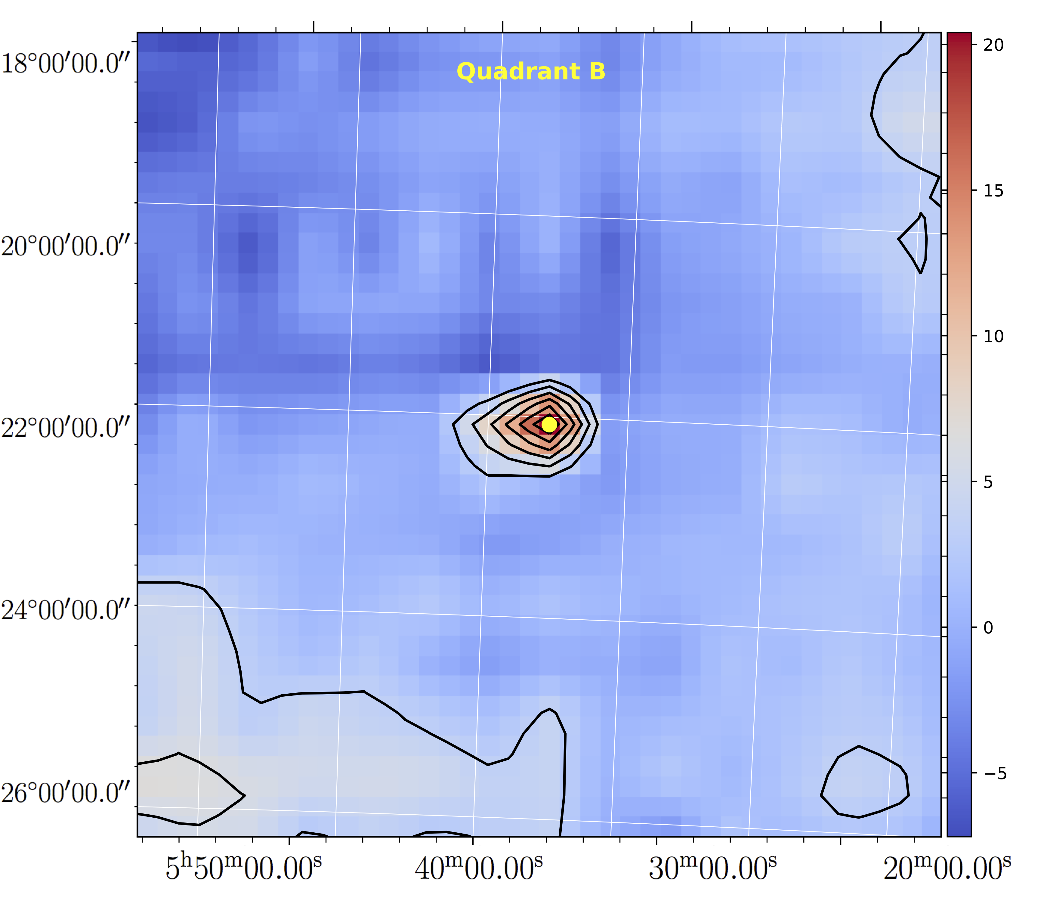
(b) Quadrant B.

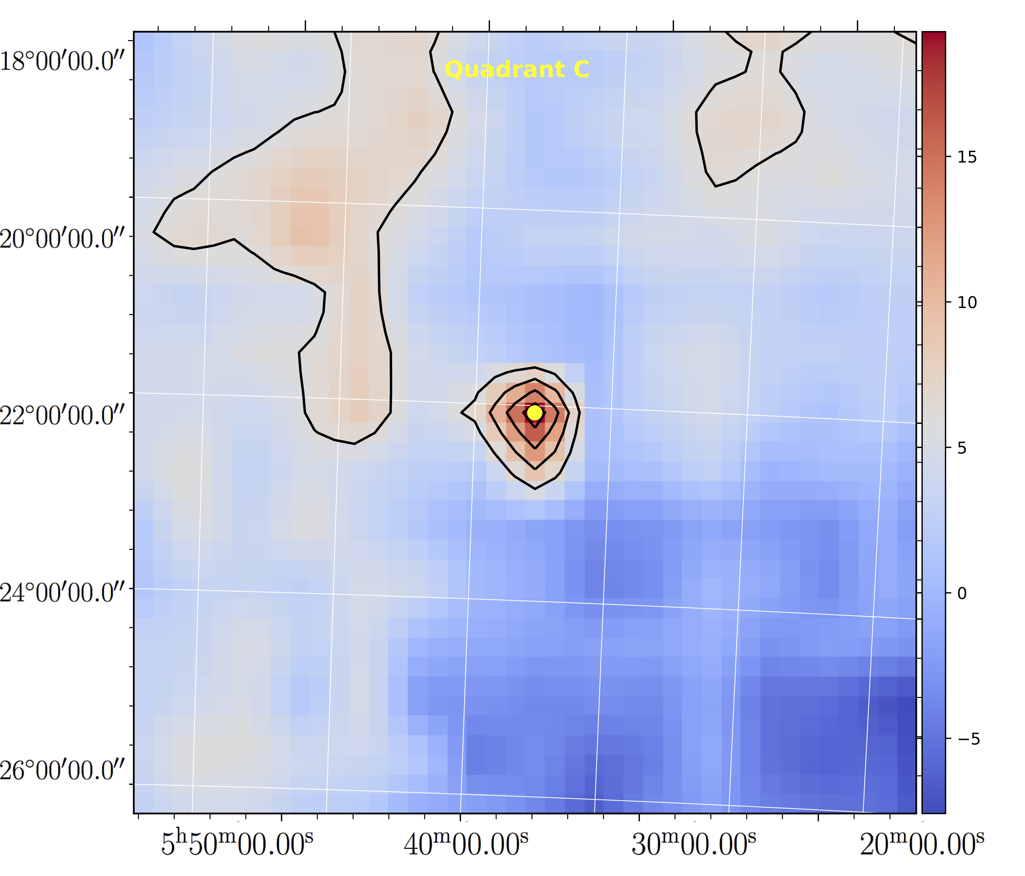
(c) Quadrant C.

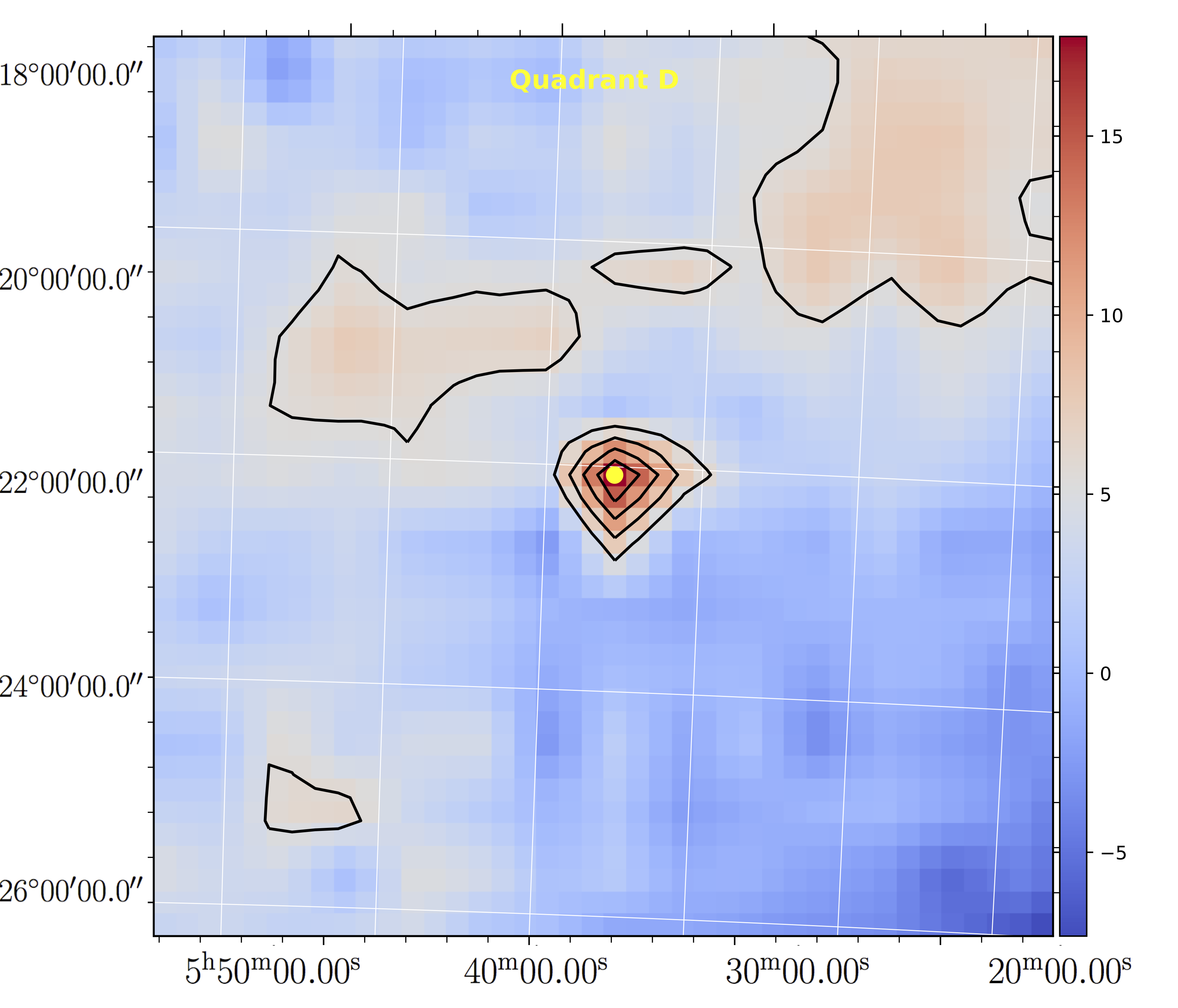
(d) Quadrant D.

Figure 21: Reconstructed sky images using the shadow library corrected for mask shifts by Balanced cross-correlation technique

Figure 21 shows the sky images reconstructed using the balanced cross-correlation. The reconstruction is performed using the shadow library corrected for the mask shift. In reconstructed images, the source is now at the expected location and also the extension in quadrant B is reduced to a great extent.

4 Conclusions

We have described the on-ground calibration and in-flight calibration performed for the imaging performance of CZTI. Using the qualification model, we verified the design of the CZTI coded mask and reconstruction algorithms. We verified that the performance of the CZTI meets the design goal of imaging resolution 8 arcmin or better. During the in-flight calibration, we found that there is a misalignment between the detector and the mask in three of its four quadrants. The estimated mask shift with respect to the detector in quadrant B was $-1.45$ mm in the X-direction, while those in quadrants C and D were +1.68 mm and +1.50 mm respectively in the Y direction. We mitigated the effect of this misalignment by modifying the algorithms employed for image reconstruction.

References

- Aschenbach (2009) Aschenbach, B. 2009, Experimental Astronomy, 26, 95
- Barthelmy . (2005) Barthelmy, S. D., Barbier, L. M., Cummings, J. R., . 2005, Space Science Reviews, 120, 143
- Bhalerao . (2017) Bhalerao, V., Bhattacharya, D., Vibhute, A., . 2017, Journal of Astrophysics and Astronomy, 38, 31
- Bhattacharya (2006) Bhattacharya, D. 2006, Advances in Space Research, 38, 2999
- Caroli . (1987) Caroli, E., Stephen, J. B., Di Cocco, G., Natalucci, L., & Spizzichino, A. 1987, Space Science Reviews, 45, 349
- Dey . (2006) Dey, N., Blanc-Feraud, L., Zimmer, C., . 2006, Microscopy Research and Technique, 69, 260
- Fenimore & Cannon (1978) Fenimore, E. E., & Cannon, T. M. 1978, Appl. Opt., 17, 337
- Godet . (2014) Godet, O., Nasser, G., Atteia, J. ., . 2014, in Society of Photo-Optical Instrumentation Engineers (SPIE) Conference Series, Vol. 9144, Space Telescopes and Instrumentation 2014: Ultraviolet to Gamma Ray, 914424
- Goldwurm . (2003) Goldwurm, A., David, P., Foschini, L., . 2003, Astronomy and Astrophysics, 411, L223
- Harrison . (2013) Harrison, F. A., Craig, W. W., Christensen, F. E., . 2013, Astrophysical Journal, 770, 103
- in’t Zand (1992) in’t Zand, J. J. M. 1992, PhD thesis, Space Research Organization Netherlands, Sorbonnelaan 2, 3584 CA Utrecht, The Netherlands
- Jager . (1997) Jager, R., Mels, W. A., Brinkman, A. C., . 1997, Astronomy and Astrophysics Supplement Series, 125, 557
- Lucy (1974) Lucy, L. B. 1974, The Astronomical Journal, 79, 745
- Ramadevi . (2017) Ramadevi, M. C., Seetha, S., Bhattacharya, D., . 2017, Experimental Astronomy, 44, 11
- Rao . (2017) Rao, A. R., Bhattacharya, D., Bhalerao, V. B., Vadawale, S. V., & Sreekumar, S. 2017, ArXiv e-prints, arXiv:1710.10773
- Rao . (2016) Rao, A. R., Chand, V., Hingar, M. K., . 2016, Astrophysical Journal, 833, 86
- Richardson (1972) Richardson, W. H. 1972, J. Opt. Soc. Am., 62, 55
- Segreto . (2010) Segreto, A., Cusumano, G., Ferrigno, C., . 2010, Astronomy and Astrophysics, 510, A47
- Shankar & Bhattacharya (2003) Shankar, B., & Bhattacharya, D. 2003, Bulletin of The Astronomical Society of India - BULL ASTRON SOC INDIA, 31, 491
- Singh . (2014) Singh, K. P., Tandon, S. N., Agrawal, P. C., . 2014, in Proceedings of SPIE, Vol. 9144, Space Telescopes and Instrumentation 2014: Ultraviolet to Gamma Ray, 91441S
- Singh . (2017) Singh, K. P., Stewart, G. C., Westergaard, N. J., . 2017, Journal of Astrophysics and Astronomy, 38, 29
- Skinner (1984) Skinner, G. K. 1984, Nuclear Instruments and Methods in Physics Research A, 221, 33
- Skinner . (1987) Skinner, G. K., Ponman, T. J., Hammersley, A. P., & Eyles, C. J. 1987, Astrophysics and Space Science, 136, 337
- Tandon . (2017) Tandon, S. N., Subramaniam, A., Girish, V., . 2017, The Astronomical Journal, 154, 128
- Vadawale . (2016) Vadawale, S. V., Rao, A. R., Bhattacharya, D., . 2016, in Society of Photo-Optical Instrumentation Engineers (SPIE) Conference Series, Vol. 9905, Space Telescopes and Instrumentation 2016: Ultraviolet to Gamma Ray, 99051G
- Winkler . (2003) Winkler, C., Courvoisier, T. J. L., Di Cocco, G., . 2003, Astronomy and Astrophysics, 411, L1
- Yadav . (2016) Yadav, J. S., Agrawal, P. C., Antia, H. M., . 2016, in Society of Photo-Optical Instrumentation Engineers (SPIE) Conference Series, Vol. 9905, Space Telescopes and Instrumentation 2016: Ultraviolet to Gamma Ray, 99051D