A fast iterative PDE-based algorithm for feedback controls of nonsmooth mean-field control problems

Abstract. A PDE-based accelerated gradient algorithm is proposed to seek optimal feedback controls of McKean-Vlasov dynamics subject to nonsmooth costs, whose coefficients involve mean-field interactions both on the state and action. It exploits a forward-backward splitting approach and iteratively refines the approximate controls based on the gradients of smooth costs, the proximal maps of nonsmooth costs, and dynamically updated momentum parameters. At each step, the state dynamics is realized via a particle approximation, and the required gradient is evaluated through a coupled system of nonlocal linear PDEs. The latter is solved by finite difference approximation or neural network-based residual approximation, depending on the state dimension. Exhaustive numerical experiments for low and high-dimensional mean-field control problems, including sparse stabilization of stochastic Cucker-Smale models, are presented, which reveal that our algorithm captures important structures of the optimal feedback control, and achieves a robust performance with respect to parameter perturbation.

Key words. Controlled McKean–Vlasov diffusion, optimal gradient method, monotone scheme, neural network, sparse control, stochastic Cucker-Smale model.

AMS subject classifications. 49N80, 60H35, 35Q93, 93A16

1 Introduction

In this article, we propose a class of iterative methods for solving mean-field control (MFC) problems, where the state dynamics and cost functions depend upon the joint law of the state and the control processes. Let $T>0$ be a given terminal time, $W=(W_{t})_{t\in[0,T]}$ be an $n$-dimensional Brownian motion defined on the probability space $(\Omega,\mathcal{F},{\mathbb{P}})$, $\mathbb{F}=(\mathcal{F}_{t})_{t\in[0,T]}$ the natural filtration of $W$ augmented with an independent $\sigma$-algebra $\mathcal{F}_{0}$, and $\mathcal{H}^{2}({\mathbb{R}}^{k})$ be the set of admissible controls containing all ${\mathbb{R}}^{k}$-valued square integrable $\mathbb{F}$-progressively measurable processes. For a given $\mathcal{F}_{0}$-measurable initial state $\xi\in L^{2}(\Omega;\mathbb{R}^{d})$ and a control $\alpha\in\mathcal{H}^{2}({\mathbb{R}}^{k})$, we consider the state process governed by the following controlled McKean–Vlasov diffusion:

$$\mathrm{d}X_{t}=b(t,X_{t},\alpha_{t},\mathcal{L}_{(X_{t},\alpha_{t})})\,\mathrm{d}t+\sigma(t,X_{t},\alpha_{t},\mathcal{L}_{(X_{t},\alpha_{t})})\,\mathrm{d}W_{t},\;t\in[0,T];\quad X_{0}=\xi,$$ (1.1)

where $b:[0,T]\times{\mathbb{R}}^{d}\times{\mathbb{R}}^{k}\times\mathcal{P}_{2}({\mathbb{R}}^{d}\times{\mathbb{R}}^{k})\to{\mathbb{R}}^{d}$ and $\sigma:[0,T]\times{\mathbb{R}}^{d}\times{\mathbb{R}}^{k}\times\mathcal{P}_{2}({\mathbb{R}}^{d}\times{\mathbb{R}}^{k})\to{\mathbb{R}}^{d\times n}$ are sufficiently regular functions such that (1.1) admits a unique square integrable solution $X^{\alpha}$. The value function of the optimal control problem is defined by

$$J^{\star}(\xi)=\inf_{\alpha\in\mathcal{H}^{2}(\mathbb{R}^{k})}J(\alpha;\xi),\quad\textnormal{with}\;J(\alpha;\xi)=\mathbb{E}\bigg{[}\int_{0}^{T}\Big{(}f(t,X^{\alpha}_{t},\alpha_{t},\mathcal{L}_{(X^{\alpha}_{t},\alpha_{t})})+\ell(\alpha_{t})\Big{)}\,\mathrm{d}t+g(X^{\alpha}_{T},\mathcal{L}_{X^{\alpha}_{T}})\bigg{]},$$ (1.2)

where $f:[0,T]\times{\mathbb{R}}^{d}\times{\mathbb{R}}^{k}\times\mathcal{P}_{2}({\mathbb{R}}^{d}\times{\mathbb{R}}^{k})\to{\mathbb{R}}$, $g:{\mathbb{R}}^{d}\times\mathcal{P}_{2}({\mathbb{R}}^{d})\to{\mathbb{R}}$ are differentiable functions of at most quadratic growth, and $\ell:\mathbb{R}^{k}\to\mathbb{R}\cup\{\infty\}$ is a proper, lower semicontinuous and convex function. Above and hereafter, $\mathcal{L}_{U}$ denotes the law of a random variable $U$, and $\mathcal{P}_{2}(E)$ denotes the Wasserstein space of probability measures on the Euclidean space $E$ with finite second moment.

The above MFC problem extends classical stochastic control problems by allowing the mean-field interactions through the joint distribution of the state and control processes. It describes large population equilibria of interacting individuals controlled by a central planner, and plays an important role in economics [12, 1, 4], production management [31], biology [20, 9, 5] and social interactions [2, 3, 4]. Moreover, the extended real-valued function $\ell$ in (1.2) includes important examples such as characteristic functions of convex sets representing control constraints [1, 47], $\ell_{1}$-norm based regularizations used to induce sparsity or switching properties of the optimal control [20, 9], and entropy regularizations in machine learning [53, 33].

To solve (1.1)-(1.2), we aim to construct an optimal (decentralized) feedback control, i.e., a sufficiently regular function $\phi^{\star}:[0,T]\times{\mathbb{R}}^{d}\to{\mathbb{R}}^{k}$ such that the corresponding controlled dynamics (1.1) (with $\alpha_{t}=\phi^{\star}(t,X_{t})$) admits a unique solution $X^{\phi^{\star}}$ and $J^{\star}(\xi)=J(\phi^{\star}(\cdot,X^{\phi^{\star}}_{\cdot}),\xi)$. The existence of such feedback controls has been shown in [47] (see also [21, Section 6.4] for special cases without mean-field interactions through control variables). The main advantage of a feedback strategy is that implementing the optimal control reduces to simple function evaluation at the current state of the system. Moreover, a feedback control allows us to interpret the mechanism of the optimal control. This is particularly important for economics and social science [42], where one would like to understand the cause of a decision, and explain its dependence on the state dynamics and the objective function. A feedback control also allows us to analyze the failure of certain control policies for fault diagnosis.

Existing numerical methods for MFC problems and their limitations.

As analytical solutions to optimal feedback controls of (1.1)-(1.2) are rarely available, numerical schemes for solving such control problems become vital. Due to the nonlinear dependence on the marginal laws, it is difficult to follow the classical dynamic programming (DP) approach for constructing optimal feedback controls. The main challenge here is that to construct feedback controls, DP requires us to find derivatives of solutions to an infinite-dimensional Hamilton-Jacobi-Bellman (HJB) partial differential equation (PDE) defined on $[0,T]\times\mathcal{P}_{2}({\mathbb{R}}^{d})$ (see e.g., [46]), which is computationally intractable. Hence, most existing numerical methods are based on the optimization interpretation of (1.1)-(1.2).

The most straightforward approach for solving (1.1)-(1.2) is to restrict the optimization over feedback controls within a prescribed parametric family, i.e., the so-called policy gradient (PG) method (see e.g., [22]). It approximates the optimal feedback control in a parametric form depending on weights $\theta$ (for instance a deep neural network), and then seeks the optimal approximation by performing gradient descent of $J$ with respect to the weights $\theta$ based on simulated trajectories of the state process. By exploiting an efficient neural network representation of the feedback control, the PG method can be adapted to solve MFC problems with high-dimensional state processes.

However, the PG method has two serious drawbacks, especially for solving control problems with nonlinear dynamics and nonsmooth costs in (1.1)-(1.2). Firstly, as the loss functional $J$ is nonconvex and nonsmooth in the weights $\theta$ of the numerical feedback controls, there is no theoretical guarantee on the convergence of the PG method for solving nonsmooth MFC problems. In practice, even though the PG method may minimize the loss function reasonably well, the resulting approximate feedback control often fails to capture important structural features of the optimal feedback control, and consequently lacks the capability to provide sufficient insights of the optimal decision; see Figures 6, 7 and 9 in Section 5.2.2 where the PG method ignores the temporal and spatial nonlinearity and the sparsity of the optimal controls. Secondly, as the PG method computes approximate feedback controls based purely on sample trajectories of the state dynamics, it cannot recover optimal feedback controls outside the support of the optimal state process. Consequently, the performance of the approximate feedback control in general can be very sensitive to perturbations of the (random) initial state $\xi$ of (1.1); see Section 5.1 for details. This is undesirable for practical applications of MFC problems, as the initial condition $\xi$ describes the asymptotic regime of initial conditions of a large number of players, and often cannot be observed exactly.

Another approach is to solve the optimality systems arising from applying the Pontryagin Maximum Principle (PMP) to (1.1)-(1.2). Existing works consider special cases with neither nonsmooth costs nor mean-field interactions through control variables, and design numerical methods based on either a probabilistic or deterministic formulation (see e.g., [21, Section 6.2.4]). The probabilistic formulation represents an optimal control $\alpha^{\star}\in\mathcal{H}^{2}({\mathbb{R}}^{k})$ as $\alpha^{\star}_{t}=\hat{\alpha}(t,X^{\alpha^{\star}}_{t},\mathcal{L}_{X^{\alpha^{\star}}_{t}},Y^{\alpha^{\star}}_{t},Z^{\alpha^{\star}})$ for $\,\text{\rm{d}}t\otimes\,\text{\rm{d}}{\mathbb{P}}$-a.e., with $\hat{\alpha}$ being the pointwise minimizer of an associated Hamiltonian $\mathcal{H}$, and $(X^{\alpha^{\star}},Y^{\alpha^{\star}},Z^{\alpha^{\star}})$ being the solution to a coupled forward-backward stochastic differential equation (FBSDE) depending on $\hat{\alpha}$. The coupled FBSDE can be solved by first representing the solution in terms of grid functions [6, 48], binomial trees [6] or neural networks [27, 22, 29], and then employing regression methods to obtain the optimal approximation. Similarly, the deterministic formulation represents an optimal feedback control $\phi^{\star}$ as $\phi^{\star}(t,x)=\bar{\alpha}(t,x,\mu^{\star}_{t},(\nabla_{x}v)(t,x),(\textrm{Hess}_{x}v)(t,x))$ for all $(t,x)\in[0,T]\times{\mathbb{R}}^{d}$. Here $\bar{\alpha}$ is the pointwise minimizer of an associated Hamiltonian $\mathscr{H}$ (possibly different from $\mathcal{H}$), and $(\mu^{\star},v)$ satisfy a coupled Fokker-Planck (FP)-HJB PDE system depending on $\bar{\alpha}$, which consists of a nonlinear FP equation for the marginal distribution $\mu^{\star}$ of the optimal state process, and of a nonlinear HJB equation for the adjoint variable $v$. The FP-HJB system can then be solved by finite difference methods as in [2, 3, 4] or by neural network methods as in [23].

We observe, however, that the above PMP approach suffers from the following limitations. Firstly, the derivation of the optimality systems relies heavily on the analytic expression of pointwise minimizers of the Hamiltonians, which may not be available for general control problems. More crucially, as pointed out in [1], when there is a nonlinear dependence on the law of the control, the PMP in general cannot be expressed in terms of a pointwise minimization of Hamiltonian (see [47] for a detailed investigation of this issue). These factors prevent us from applying the PMP approach to solve (1.1)-(1.2) with general cost functions and control interactions. Secondly, similar to the PG method, solving the coupled FBSDE via regression focuses mainly along trajectories of the optimal state, and consequently would result in an approximate feedback control that is sensitive to perturbation of the initial state (see Section 5.1). Finally, solutions to the nonlinear FP equation in general only exist in the sense of distributions and often admit temporal and spatial singularity. This creates significant numerical challenges, especially when the diffusion coefficient $\sigma$ of (1.1) is degenerate (as in most kinetic models) or the initial state $\xi$ has a singular density; see Section 5 for concrete examples. In particular, in the high-dimensional setting, one may need to employ neural networks with complex structures to approximate such irregular solutions, which subsequently results in challenging optimization problems for training the networks.

Our contributions and related works.

This paper proposes a class of iterative algorithms to construct optimal feedback controls for nonsmooth MFC problems (1.1)-(1.2).

• We construct a sequence of feedback controls $\phi^{m}:[0,T]\times{\mathbb{R}}^{d}\to{\mathbb{R}}^{k}$ whose realized control processes minimize the functional $J$. This is done by following an accelerated gradient descent algorithm, which extends the forward-backward splitting algorithm for finite-dimensional minimization problems in [15] to the present (infinite-dimensional) nonsmooth MFC problems. At each iteration with given feedback control, we evaluate the gradient of the smooth costs at the corresponding realized control process, and update the feedback control by incorporating the gradient information, the proximal map of the nonsmooth cost $\ell$, and an explicit dynamically updated momentum parameter.

  The proposed accelerated proximal gradient approach has the following advantages in solving (1.1)-(1.2): (i) unlike the aforementioned PMP approach, our algorithm requires neither (pointwise) analytical minimization of the Hamiltonian nor deriving the optimality systems, and hence can be applied to MFC problems with general mean-field interactions through the control variables; (ii) our algorithm shares the same computational complexity as the gradient-based algorithms in [45, 7, 53, 36] (by requiring one gradient evaluation per iteration), but enjoys an accelerated convergence rate and can handle general convex nonsmooth costs, including $\ell_{1}$-regularizers and control constraints. In fact, such an accelerated gradient iteration is known to be an optimal first order (gradient) method (in the sense of complexity analysis) for minimizing finite-dimensional nonsmooth functions [15]; (iii) our method represents the control iterates in a feedback form (cf., [7, 53, 36] which update controls as stochastic processes), and avoids the curse of dimensionality in the gradient evaluation as the number of iterations tends to infinity (see Section 2 for details).

• We present a practical implementation of the above accelerated gradient algorithm by combining Monte Carlo and PDE approaches. At each iteration, the state dynamics with a given feedback control is realized by using a particle approximation and Euler-Maruyama timestepping scheme, and the required gradient is computed by solving a coupled system of nonlocal linear PDEs, whose coefficients depend on the empirical measure of the particle system. The coupled PDE system is then solved with two different approaches depending on the state dimension $d$ in (1.1), in order to balance the efficiency and computation complexity. In the low-dimensional setting (say $d\leq 2$), we discretize the coupled PDE system by a class of semi-implicit monotone finite difference approximations. To accommodate the curse of dimensionality with large state dimension, we also propose a residual approximation approach to solve the coupled PDE system, in which the numerical solution is decomposed into a pre-determined candidate solution and an unknown residual term. The computation of the residual term is addressed by a mesh-free method based on neural network approximation and stochastic optimization algorithms, such as the Stochastic Gradient Descent (SGD) algorithm or its variants.

  The proposed algorithm combines the advantages of probabilistic and deterministic approaches. Firstly, the particle approximation allows for efficient computation of the marginal distribution of the state process and avoids the numerical challenge in solving a nonlinear FP equation (cf., [2, 3, 4, 23]). This is particularly relevant for high-dimensional MFC problems with degenerate diffusion coefficients or irregular initial distribution (see Section 5). Secondly, by exploiting the PDE formulation of the gradient evaluation, our algorithm recovers the optimal feedback control on the entire computational domain, rather than merely along the trajectories of the optimal state (cf., the probabilistic methods in [6, 22, 29, 48]). This allows us to capture important structures of the optimal control and achieve a robust performance with parameter uncertainty (see Section 5). As alluded to earlier, such an accurate approximation of the optimal feedback control is practically important for mathematical modelling and fault diagnosis in engineering. Finally, instead of directly applying SGD to high-dimensional PDE systems as in [52, 23], the proposed residual approximation approach leverages available efficient solvers to compute the dominant part of solutions (see e.g., the Riccati-based solvers in [31, 5]), and employs a small number of SGD iterations to fit the residual term. This significantly accelerates the convergence of the algorithm for solving high-dimensional MFC problems (see Figure 8).

• We demonstrate the effectiveness of the algorithm through extensive numerical experiments. This includes a two-dimensional nonsmooth MFC problem arising from portfolio liquidation with trade crowding, and a six-dimensional nonsmooth nonconvex MFC problem arising from sparse consensus control of stochastic Cucker-Smale models. Our experiments show that the resulting approximate feedback control correctly captures the temporal/spatial nonlinearity and the sparsity of the optimal control, and achieves a robust performance in the presence of initial state perturbation.

The rest of the paper is organized as follows. Section 2 describes our numerical methodology, including the accelerated proximal gradient iteration, the particle system for the state process, and the PDE system for the gradient evaluation. We then propose a class of finite difference approximations in Section 3 and neural network-based residual approximations in Section 4 to solve the PDE systems. In Section 5, we present exhaustive numerical experiments for multidimensional nonsmooth nonconvex MFC problems, which demonstrate that the proposed algorithm leads to more accurate and stable feedback controls than the aforementioned PG method and the PMP method.

2 Fast iterative PDE-based method for MFCs

In this section, we propose a class of Markovian accelerated proximal gradient methods for MFC problems with nonsmooth running costs.

2.1 Accelerated gradient method with open-loop control

We start by interpreting the MFC problem (1.1)-(1.2) as a nonsmooth optimization problem over the Hilbert space $\mathcal{H}^{2}({\mathbb{R}}^{k})$:

$$\inf_{\alpha\in\mathcal{H}^{2}(\mathbb{R}^{k})}(F(\alpha)+G(\alpha)),$$ (2.1)

with the functionals $F:\mathcal{H}^{2}(\mathbb{R}^{k})\to{\mathbb{R}}$ and $G:\mathcal{H}^{2}(\mathbb{R}^{k})\to{\mathbb{R}}\cup\{\infty\}$ defined as follows: for all $\alpha\in\mathcal{H}^{2}({\mathbb{R}}^{k})$,

$$F(\alpha)\coloneqq\mathbb{E}\bigg{[}\int_{0}^{T}f(t,X^{\alpha}_{t},\alpha_{t},\mathcal{L}_{(X^{\alpha}_{t},\alpha_{t})})\,\mathrm{d}t+g(X^{\alpha}_{T},\mathcal{L}_{X^{\alpha}_{T}})\bigg{]},\quad G(\alpha)\coloneqq\mathbb{E}\bigg{[}\int_{0}^{T}\ell(\alpha_{t})\,\,\text{\rm{d}}t\bigg{]},$$ (2.2)

where $X^{\alpha}\in\mathcal{S}^{2}({\mathbb{R}}^{d})$ is the state process controlled by $\alpha$ satisfying (1.1). It is clear that $G:\mathcal{H}^{2}(\mathbb{R}^{k})\to{\mathbb{R}}\cup\{\infty\}$ is convex due to the convexity of $\ell$. Moreover, by [1, Lemma 3.1] and by assuming the differentiability of $(b,\sigma,f)$, $F:\mathcal{H}^{2}(\mathbb{R}^{k})\to{\mathbb{R}}$ is Fréchet differentiable with the derivative $\nabla F:\mathcal{H}^{2}(\mathbb{R}^{k})\to\mathcal{H}^{2}(\mathbb{R}^{k})$ such that for all $\alpha\in\mathcal{H}^{2}({\mathbb{R}}^{k})$,

$${(\nabla F)(\alpha)_{t}}=(\partial_{a}H)(t,X^{\alpha}_{t},\alpha_{t},\mathcal{L}_{(X^{\alpha}_{t},\alpha_{t})},Y^{\alpha}_{t},Z^{\alpha}_{t})+\tilde{\mathbb{E}}[(\partial_{\nu}H)(t,\tilde{X}^{\alpha}_{t},\tilde{\alpha}_{t},\mathcal{L}_{(X^{\alpha}_{t},\alpha_{t})},\tilde{Y}^{\alpha}_{t},\tilde{Z}^{\alpha}_{t})(X^{\alpha}_{t},\alpha_{t})],$$ (2.3)

$\,\text{\rm{d}}t\otimes\,\text{\rm{d}}{\mathbb{P}}$-a.e., where $H:[0,T]\times\mathbb{R}^{d}\times\mathbb{R}^{k}\times\mathcal{P}_{2}(\mathbb{R}^{d}\times\mathbb{R}^{k})\times\mathbb{R}^{d}\times\mathbb{R}^{d\times n}\to\mathbb{R}$ is the Hamiltonian defined by:

$$H(t,x,a,\eta,y,z)\coloneqq\left\langle b(t,x,a,\eta),y\right\rangle+\left\langle\sigma(t,x,a,\eta),z\right\rangle+f(t,x,a,\eta),$$ (2.4)

and $(Y^{\alpha},Z^{\alpha})$ are square integrable adapted adjoint processes such that for all $t\in[0,T]$,

$$\begin{split}\mathrm{d}Y^{\alpha}_{t}&=-\Big{(}(\partial_{x}H)(t,X^{\alpha}_{t},\alpha_{t},\mathcal{L}_{(X^{\alpha}_{t},\alpha_{t})},Y^{\alpha}_{t},Z^{\alpha}_{t})\\ &\qquad+\tilde{\mathbb{E}}[(\partial_{\mu}H)(t,\tilde{X}^{\alpha}_{t},\tilde{\alpha}_{t},\mathcal{L}_{(X^{\alpha}_{t},\alpha_{t})},\tilde{Y}^{\alpha}_{t},\tilde{Z}^{\alpha}_{t})(X^{\alpha}_{t},\alpha_{t})]\Big{)}\,\,\text{\rm{d}}t+Z^{\alpha}_{t}\,\,\text{\rm{d}}W_{t},\\ Y^{\alpha}_{T}&=(\partial_{x}g)(X^{\alpha}_{T},\mathcal{L}_{X^{\alpha}_{T}})+\tilde{\mathbb{E}}[(\partial_{\mu}g)(\tilde{X}^{\alpha}_{T},\mathcal{L}_{X^{\alpha}_{T}})(X^{\alpha}_{T})].\end{split}$$ (2.5)

Above and hereafter, we use the tilde notation to denote an independent copy of a random variable as in [1]. Moreover, for a given function $h:\mathcal{P}_{2}(\mathbb{R}^{d}\times\mathbb{R}^{k})\to\mathbb{R}$ and a measure $\eta\in\mathcal{P}_{2}(\mathbb{R}^{d}\times\mathbb{R}^{k})$ with marginals $\mu\in\mathcal{P}_{2}(\mathbb{R}^{d})$, $\nu\in\mathcal{P}_{2}(\mathbb{R}^{k})$, we denote by $\big{(}(\partial_{\mu}h)(\eta),(\partial_{\nu}h)(\eta)\big{)}(\cdot):\mathbb{R}^{n}\times\mathbb{R}^{k}\to\mathbb{R}^{n}\times\mathbb{R}^{k}$ the partial L-derivatives of $h$ with respect to the marginals; see e.g., [1, Section 2.1] or [21, Chapter 5] for detailed definitions.

Based on the above interpretation, we can design an accelerated gradient descent algorithm to find optimal controls of (1.1)-(1.2), which extends Nesterov’s accelerated proximal gradient (NAG) method (also known as the Fast Iterative Shrinkage-Thresholding Algorithm [15]) to the present infinite-dimensional setting. Roughly speaking, at each iteration, we evaluate the gradient of the smooth functional $F$ at a given control, compute the proximal operator of the nonsmooth functional $G$, and incorporate Nesterov momentum in the control update, in order to accelerate the convergence of the algorithm.

More precisely, let $\alpha^{0}\in\mathcal{H}^{2}(\mathbb{R}^{k})$ be the initial guess of the optimal control, and $\tau>0$ be a chosen stepsize. We consider the following sequences $(\alpha^{m})_{m\in\mathbb{N}}$ and $(\beta^{m})_{m\in\mathbb{N}}$ such that $\beta^{0}=\alpha^{0}$ and for each $m\in\mathbb{N}\cup\{0\}$,

$$\alpha_{t}^{m+1} =\text{prox}_{\tau\ell}\left(\beta_{t}^{m}-\tau(\nabla F)(\beta^{m})_{t}\right),\quad\beta_{t}^{m+1}=\alpha_{t}^{m+1}+\frac{m}{m+3}(\alpha_{t}^{m+1}-\alpha_{t}^{m})$$ (2.6)

$\mathrm{d}t\otimes\mathrm{d}\mathbb{P}$-a.e., where $(\nabla F)(\beta^{m})$ is defined by (2.3), and $\operatorname*{prox}_{\tau\ell}:{\mathbb{R}}^{k}\to{\mathbb{R}}^{k}$ is the proximal map of $\tau\ell:{\mathbb{R}}^{k}\to{\mathbb{R}}\cup\{\infty\}$ such that

$$\textrm{prox}_{\tau\ell}(a)=\arg\min_{z\in{\mathbb{R}}^{k}}\left(\frac{1}{2}|z-a|^{2}+\tau\ell(z)\right),\quad a\in{\mathbb{R}}^{k},\tau>0.$$

The ratio $\frac{m}{m+3}$ in (2.6) is often referred to as the momentum parameter. It ensures that the iteration (2.6) converges with an optimal rate for convex and smooth functionals $F$; see the first paragraph of Section 2.3 for a detailed discussion. Such a regularity condition holds in particular for commonly used linear-convex MFC problems (see e.g., [12, 1, 31, 47]). To derive (2.6), we have also exploited the structure of the nonsmooth functional $G$ and explicitly expressed the proximal operator of $G:\mathcal{H}^{2}(\mathbb{R}^{k})\to{\mathbb{R}}\cup\{\infty\}$ via a pointwise composition of the proximal map of $\ell$. For many practically important nonsmooth functions $\ell$, the proximal function $\operatorname*{prox}_{\tau\ell}$ can be evaluated either analytically (see e.g., [13, Chapter 6]) or approximately by efficient numerical methods (see [51] and the references therein).

However, we observe that the non-Markovian nature of $(\alpha^{m})_{m\in\mathbb{N}}$ creates an essential difficulty in solving for the adjoint processes $(Y^{m},Z^{m})_{m\in\mathbb{N}}$, and hence in evaluating $(\nabla F)(\beta^{m})$ for each $m$. This prevents us from implementing the updates (2.6) in the pairwise sense as for gradient-based algorithms for deterministic optimal control problems (see e.g., [8]). To be more precise, let us initialize the iterates (2.6) with $\alpha^{0}=0$. Then one can express $(Y^{1},Z^{1})$ as $(Y^{0}_{t},Z^{0}_{t})=(u(t,X^{0}_{t}),v(t,X^{0}_{t}))$ for some deterministic functions $u,v$ (often called decoupling fields), and obtain the stochastic processes $(Y^{0},Z^{0})$ by computing the functions $u,v$. Hence, one easily sees that $(\alpha^{1},\beta^{1})$ are functions of $X^{0}$, and consequently, the coefficients of the state dynamics (1.1) and adjoint equations (2.5) for $(X^{1},Y^{1},Z^{1})$ would depend on both $X^{0}$ (through $\beta^{1}$) and $X^{1}$. Repeating this process, one observes that $(Y^{m},Z^{m})$ are functions of time and the enlarged system $(X^{0},\ldots,X^{m})$, whose computational complexity increases rapidly as the number of NAG iterations grows. A similar difficulty has been observed in [16] for implementing (non-Markovian) Picard iterations to solve coupled FBSDEs.

2.2 Accelerated gradient method with feedback control

To address the above difficulty, we propose a Markovian analogue of the above NAG iteration, for which the dimensions of the decoupling fields for the adjoint processes do not change with respect to the number of NAG iterations. Roughly speaking, we shall represent the control $\alpha^{m}$ as $\alpha^{m}_{t}=\phi^{m}(t,X^{m}_{t})$ with some deterministic feedback function $\phi^{m}:[0,T]\times\mathbb{R}^{d}\to\mathbb{R}^{k}$ at each iteration, which will be updated by the NAG iteration as in (2.6). More precisely, at the $m$-th iteration, we consider the following state dynamics controlled by a sufficiently regular feedback policy $\psi^{m}:[0,T]\times\mathbb{R}^{d}\to\mathbb{R}^{k}$ (which is typically different from $\phi^{m}$): $X_{0}=\xi$, and for all $t\in[0,T]$,

$$\mathrm{d}X_{t}=b(t,X_{t},\psi^{m}(t,X_{t}),\mathcal{L}_{(X_{t},\psi^{m}(t,X_{t}))})\,\mathrm{d}t+\sigma(t,X_{t},\psi^{m}(t,X_{t}),\mathcal{L}_{(X_{t},\psi^{m}(t,X_{t}))})\,\mathrm{d}W_{t}.$$ (2.7)

Let $X^{m}$ be the solution of (2.7); we then seek the adjoint processes $(Y^{m},Z^{m})$ satisfying (2.5) with $(X^{\alpha},\alpha)$ replaced by $(X^{m},\psi^{m}(\cdot,X^{m}))$, in order to evaluate the gradient of $F$ at the corresponding control process $\psi^{m}(\cdot,X^{m})$ as in (2.3). The feedback structure of $\alpha^{m}$ implies that there exist deterministic decoupling fields $u^{m}:[0,T]\times\mathbb{R}^{d}\to\mathbb{R}^{d}$ and $v^{m}:[0,T]\times\mathbb{R}^{d}\to\mathbb{R}^{d\times n}$ such that for $\mathrm{d}t\otimes\mathrm{d}\mathbb{P}$-a.e.,

$$Y^{m}_{t}=u^{m}(t,X^{m}_{t}),\quad Z^{m}_{t}=v^{m}(t,X^{m}_{t}),$$ (2.8)

This reduces the numerical approximation of $(Y^{m},Z^{m})$ to the computation of $(u^{m},v^{m})$. Once the functions $(u^{m},v^{m})$ are determined, one can compute the updated control $\alpha^{m+1}$ via the gradient descent step (2.6) with the Nesterov momentum. In fact, by virtue of the Markovian representation (2.8), we see $(\nabla F)(\psi^{m}(\cdot,X^{m}))_{t}=(\nabla F)(\psi^{m})(t,X^{m}_{t})$, $\mathrm{d}t\otimes\,\text{\rm{d}}\mathbb{P}$-a.e., with the function $(\nabla F)(\psi^{m}):[0,T]\times\mathbb{R}^{d}\to\mathbb{R}^{k}$ defined by

$$\begin{split}&(\nabla F)(\psi^{m})(t,x)\\ &\coloneqq(\partial_{a}H)(t,x,\psi^{m}(t,x),\mathcal{L}_{(X^{m}_{t},\psi^{m}(t,X^{m}_{t}))},u^{m}(t,x),v^{m}(t,x))\\ &\quad+\tilde{\mathbb{E}}[(\partial_{\nu}H)(t,\tilde{X}^{m}_{t},\psi^{m}(t,\tilde{X}^{m}_{t}),\mathcal{L}_{(X^{m}_{t},\psi^{m}(t,X^{m}_{t}))},u^{m}(t,\tilde{X}^{m}_{t}),v^{m}(t,\tilde{X}^{m}_{t}))(x,\psi^{m}(t,x))].\end{split}$$ (2.9)

This allows us to update the control $\alpha^{m+1}$ through the feedback map $\phi^{m+1}$ based on $\psi^{m}$, $u^{m}$ and $v^{m}$.

To compute the decoupling fields $(u^{m},v^{m})$ in (2.8) for each $m$, we connect them with solutions to some PDE systems. In fact, the nonlinear Feynman–Kac formula in [44] shows that, if $u^{m}$ is sufficiently smooth, then $v^{m}(t,x)=(\nabla_{x}u^{m})(t,x)\sigma(t,x,\mathcal{L}_{X^{m}_{t}})$ for all $(t,x)\in[0,T]\times\mathbb{R}^{d}$, and $u^{m}$ solves the following system of parabolic linear PDEs (depending on $\psi^{m}$ and the law of $X^{m}$):

$$(\partial_{t}u)(t,x)+(\mathscr{L}^{m}u)(t,x)=-f^{m}(t,x,u,v),$$ (2.10)

with $u(T,x)=h^{m}(x)$ and $v(t,x)=(\nabla_{x}u)(t,x)\sigma^{m}(t,x)$ for all $(t,x)\in[0,T]\times\mathbb{R}^{d}$, where $\mathscr{L}^{m}$ is the (vector-valued) differential operator such that for each $\varphi=(\varphi_{1},\ldots,\varphi_{d})\in C^{1,2}([0,T]\times\mathbb{R}^{d};\mathbb{R}^{d})$, $i\in\{1,\ldots,d\}$ and $(t,x)\in[0,T]\times\mathbb{R}^{d}$,

$$(\mathscr{L}^{m}\varphi)_{i}(t,x)=\frac{1}{2}\text{tr}\big{(}\sigma^{m}(t,x)\sigma^{m}(t,x)^{\mathsf{T}}(\textrm{Hess}_{x}\varphi_{i})(t,x)\big{)}+\langle b^{m}(t,x),(\nabla_{x}\varphi_{i})(t,x)\rangle,$$ (2.11)

with $b^{m}:[0,T]\times\mathbb{R}^{d}\to\mathbb{R}^{d}$ and $\sigma^{m}:[0,T]\times\mathbb{R}^{d}\to\mathbb{R}^{d\times n}$ given by

$$\begin{split}b^{m}(t,x)&=b(t,x,\psi^{m}(t,x),\mathcal{L}_{(X^{m}_{t},\psi^{m}(t,X^{m}_{t}))}),\\ \sigma^{m}(t,x)&=\sigma(t,x,\psi^{m}(t,x),\mathcal{L}_{(X^{m}_{t},\psi^{m}(t,X^{m}_{t}))}),\end{split}$$ (2.12)

and the functions $f^{m}$ and $h^{m}$ satisfy for all $(t,x)\in[0,T]\times{\mathbb{R}}^{d}$ (cf. (2.5)),

$$f^{m}(t,x,u,v) =(\partial_{x}H)(t,x,\psi^{m}(t,x),\mathcal{L}_{(X^{m}_{t},\psi^{m}(t,X^{m}_{t}))},u(t,x),v(t,x))$$ (2.13)

$$\quad+\tilde{\mathbb{E}}[(\partial_{\mu}H)(t,\tilde{X}^{m}_{t},\psi^{m}(t,\tilde{X}^{m}_{t}),\mathcal{L}_{(X^{m}_{t},\psi^{m}(t,X^{m}_{t}))},u(t,\tilde{X}^{m}_{t}),v(t,\tilde{X}^{m}_{t}))(x,\psi^{m}(t,x))],$$

$$h^{m}(x) =(\partial_{x}g)(x,\mathcal{L}_{X^{m}_{T}})+\tilde{\mathbb{E}}[(\partial_{\mu}g)(\tilde{X}^{m}_{T},\mathcal{L}_{X^{m}_{T}})(x)].$$ (2.14)

Concrete numerical methods for solving (2.10) will be given in Sections 3 and 4.

Here, we point out the following three features of the PDE system (2.10), which are crucial in the design of numerical methods: (i) As the Hamiltonian $H$ defined in (2.4) is affine in the components $y$ and $z$, the function $f^{m}$ is linear in $u$ and $v$, and hence (2.10) is a linear PDE system. (ii) Due to the measure dependence in $f^{m}$, (2.10) is nonlocal in the sense that the value of the solution $u^{m}$ at each point evolves based on the weighted average of other values of $u^{m}$ with respect to the marginal law $(\mathcal{L}_{X^{m}_{t}})_{t\in[0,T]}$ of the process $X^{m}$. (iii) Even though the $i$-th component of the differential operator $\mathscr{L}^{m}$ in (2.11) only involves the $i$-th component of the solution $u^{m}$, the function $f^{m}$ in (2.10) in general results in a coupling among all components of $u$ and their gradients $v$. In the special cases where the diffusion coefficient $\sigma$ of (1.1) depends only on time (see Section 5 for concrete examples), the function $f^{m}$ is independent of $v$ and hence the system (2.10) is only coupled through the solution $u^{m}$.

Algorithm 1 summarizes the Markovian NAG method for (1.1)-(1.2) based on the PDE system (2.10), which will also be referred to as the fast iterative PDE-based (FIPDE) method hereafter. In particular, the term “fast”, analogous to [15], refers to the momentum acceleration in (2.15) and indicates that Algorithm 1 converges faster than a plain gradient descent iteration over feedback controls (see Figures 5 and 6 for details).

Algorithm 1 Fast Iterative PDE-based method for MFC problems

1:  Input: Choose the initial feedback control $\phi^{0}:[0,T]\times\mathbb{R}^{d}\mapsto\mathbb{R}^{k}$ and stepsize $\tau>0$. Set $\psi^{0}=\phi^{0}$.

2:  for $m=0,1\ldots$ do

3:     Compute the law of the state process $X^{m}$ governed by (2.7).

4:     Compute the decoupling fields $(u^{m},v^{m})$ of $(Y^{m},Z^{m})$ by solving (2.10) based on the law of $X^{m}$.

5:     Update the controls such that for all $(t,x)\in[0,T]\times\mathbb{R}^{d}$,

$$\begin{split}\phi^{m+1}(t,x)&=\text{prox}_{\tau\ell}\left(\psi^{m}(t,x)-\tau(\nabla F)(\psi^{m})(t,x)\right),\\ \psi^{m+1}(t,x)&=\phi^{m+1}(t,x)+\frac{m}{m+3}(\phi^{m+1}(t,x)-\phi^{m}(t,x)),\end{split}$$ (2.15)

with $(\nabla F)(\psi^{m})$ defined by (2.9).

6:  end for

We emphasize that, a key feature of the FIPDE method is that it computes the functions $(u^{m},v^{m})$ for each $(t,x)\in[0,T]\times{\mathbb{R}}^{d}$ based on a PDE formulation, in contrast to the pure data-driven algorithms in [6, 22, 29, 48], which solve $(u^{m},v^{m})$ merely along the trajectories of $X^{m}$. Hence, the FIPDE method leads to a more accurate approximation of the optimal feedback control, especially outside the support of the optimal state process of (1.1)-(1.2). In particular, the FIPDE method is capable of recovering important structural features of the optimal control, and the performance of the approximate feedback control is robust with respect to perturbation of model parameters; see Section 5 for a detailed comparison between the FIPDE method and several data-driven algorithms.

In practice, we represent the feedback maps $(\phi^{m},\psi^{m})_{m\in\mathbb{N}}$ and the decoupling fields $(u^{m},v^{m})_{m\in\mathbb{N}}$ in suitable parametric forms, whose precise choices depend on the dimension of the problem and the numerical methods used to solve the PDE system (2.10) (see Sections 3 and 4 for details). Given a parameterized feedback map $\psi^{m}$, the law of the controlled state process $X^{m}$ in Step 3 of Algorithm 1 can be approximated by a particle method and an Euler-Maruyama discretization of (2.7). For instance, let $N\in\mathbb{N}$ be the number of particles and $\{0=t_{0}<\ldots<t_{M}=T\}$ a partition of $[0,T]$ with time stepsize $\Delta t=T/M$ for some $M\in\mathbb{N}$. Then we consider the discrete-time interacting particle system $(X^{l,N}_{t})_{t\in[0,T]}$, $l=1,\ldots,N$, such that $X^{l,N}_{0}=\xi^{l}$, for $j=0,\ldots,M-1$ and $t\in[t_{j},t_{j+1})$, $X^{l,N}_{t}=X^{l,N}_{t_{j}}$, and

$$X^{l,N}_{t_{j+1}}=X^{l,N}_{t_{j}}+b(t_{j},X^{l,N}_{t_{j}},\psi^{m}(t_{j},X^{l,N}_{t_{j}}),\mu^{X,\psi^{m}}_{N,t_{j}})\Delta t+\sigma(t_{j},X^{l,N}_{t_{j}},\psi^{m}(t_{j},X^{l,N}_{t_{j}}),\mu^{X,\psi^{m}}_{N,t_{j}})\Delta W_{j}^{l},$$ (2.16)

with $\mu^{X,\psi^{m}}_{N,t_{j}}(\mathrm{d}x)=\frac{1}{N}\sum_{l=1}^{N}\delta_{(X^{l,N}_{t_{j}},\psi^{m}(t_{j},X^{l,N}_{t_{j}}))}(\mathrm{d}x)$, where $(\xi^{l})_{l=1,\ldots,N}$ and $(W^{l})_{l=1,\ldots,N}$ are independent copies of $\xi$ and $W$, respectively, $\Delta W_{j}^{l}=W^{l}_{t_{j+1}}-W^{l}_{t_{j}}$ for all $j,l$, and $\delta_{x}$ denotes the Dirac measure supported at $x$ for all $x\in\mathbb{R}^{d}$.

Compared with the deterministic methods in [2, 3, 4, 23], (2.16) avoids the numerical challenge in solving the nonlinear FP equation, and allows for efficient computation of the marginal distribution of the state process, especially for MFC problems (1.1)-(1.2) with degenerate diffusion coefficient $\sigma$ or initial state $\xi$ with singular density. In fact, it is well-known that, for sufficiently regular feedback maps $\psi^{m}$, the empirical measure $\mu^{X,\psi^{m}}_{N}$ converges to the law of $(X^{m},\psi^{m}(\cdot,X^{m}))$ in the Wasserstein metric as $M,N$ tend to infinity; see also [19, 10] for the convergence rates of (2.16) in terms of $M$ and $N$. For our numerical experiments in Section 5, we choose sufficiently large $M$ and $N$ such that the presented results are not influenced by those choices.

As numerical approximations of (2.7) are relatively well-understood, in the subsequent sections, we focus on the numerical approximations of the PDE system (2.10) with given parameterized feedback function $\psi^{m}$ and empirical approximations $\mu^{X,\psi^{m}}_{N,\cdot}$ of the law of $(X^{m},\psi^{m}(\cdot,X^{m}))$. In particular, we shall propose a class of monotone schemes in Section 3 for (2.10) with spatial dimension $d\leq 3$, and neural network-based schemes in Section 4 for the high-dimensional setting.

2.3 Convergence of gradient methods for open-loop and feedback controls

The convergence of the iteration (2.6) can be established by extending the analysis in [15] to the present infinite-dimensional setting. Indeed, by following similar arguments as in [15, Theorem 4.4], one can prove that, if the functional $F:\mathcal{H}^{2}({\mathbb{R}}^{k})\to{\mathbb{R}}\cup\{\infty\}$ in (2.2) is convex and its derivative $\nabla F:\mathcal{H}^{2}({\mathbb{R}}^{k})\to\mathcal{H}^{2}({\mathbb{R}}^{k})$ in (2.3) is Lipschitz continuous, then for sufficiently small stepsize, the corresponding costs $(J(\alpha^{m}))_{m\in\mathbb{N}}$ of the sequence $(\alpha^{m})_{m\in\mathbb{N}}$ converges to the optimal cost $J^{\star}$ in (1.2) with the sublinear rate $\mathcal{O}(m^{-2})$. This is the optimal convergence rate of gradient-based algorithms with at most one gradient evaluation for each iteration (see [15] and references therein). The same convergence rate still holds when the controls are updated with approximate proximal operators, provided that the errors made in the calculation of the proximal operator decrease at appropriate rates [51].

For nonconvex $F$, it is well-known that gradient-based algorithms in general can only find critical points. The extrapolation step in (2.6) further compounds the complexity, as $J(\beta^{m})$ may be arbitrarily larger than $J(\alpha^{m})$, especially when $F$ is oscillatory. Consequently, [14, 40, 30, 41] introduced additional monitoring steps to (2.6) to ensure a sufficient descent of the function values at each iteration. They proved that the modified algorithms generate iterates whose limit points are critical points. However, our numerical results in Section 5.2 indicate that even for nonconvex control problems, the control strategies from the unmodified NAG iteration often perform reasonably well.

Analysing the convergence of gradient methods with feedback controls (e.g., Algorithm 1) is technically more challenging. This is because the objective of a control problem is typically nonconvex with respect to feedback controls, even in the linear-quadratic setting without mean-field interaction (see [34] and the references therein). The convergence analysis also requires to investigate the regularity of the generated feedback controls, so that the state and adjoint processes are well-defined. In the more recent work [49], we analyse Algorithm 1 without the momentum step (i.e., $\psi^{m}=\phi^{m}$ for all $m$) for control problems without mean-field interaction. We identify conditions under which the algorithm generates uniform Lipschitz feedback controls $(\phi^{m})_{m\in\mathbb{N}}$, and further establish that the associated control processes converge linearly to a critical point of the functional $J$ in (1.2). The convergence result holds when the diffusion coefficient is uncontrolled, and in addition one of the following five cases is satisfied: (i) time horizon $T$ is small; (ii) running cost is sufficiently convex in control; (iii) costs depend weakly on state; (iv) control affects state dynamics weakly; (v) state dynamics is strongly dissipative. Note that the conditions allow for nonlinear state dynamics with degenerate noise, unbounded, nonconvex and nonsmooth cost functions, and unbounded action space. We refer the reader to [49] for rigorous statements of the convergence results. The proof exploits precise regularity estimates for the decoupling fields $(u^{m},v^{m})_{m\in\mathbb{N}}$ in (2.8). We conjecture that similar convergence results also hold in the mean-field setting, whose rigorous proof requires establishing the regularity of the decoupling fields in the measure component, and is left for future research.

2.4 Importance of the gradient direction in Algorithm 1

We emphasise that Algorithm 1 updates a feedback map using the Markovian representation of the functional gradient at the corresponding open-loop control (see (2.9)), instead of using the gradient of $J$ at the feedback map itself. This difference is crucial for the convergence analysis of Algorithm 1. For demonstration purposes, we assume for simplicity that there is no mean-field interaction, all variables are one-dimensional, and consider minimising the following cost (with $\ell\equiv 0$ in (1.2)):

$$J(\phi)\coloneqq\mathbb{E}\bigg{[}\int_{0}^{T}f(t,X^{\phi}_{t},\phi(t,X^{\phi}_{t}))\,\mathrm{d}t+g(X^{\phi}_{T})\bigg{]},$$ (2.17)

over all feedback maps $\phi:[0,T]\times{\mathbb{R}}\to{\mathbb{R}}$, where for each $\phi$, $X^{\phi}$ satisfies the following controlled dynamics:

$$\mathrm{d}X_{t}=b(t,X_{t},\phi(t,X_{t}))\,\mathrm{d}t+\sigma\,\mathrm{d}W_{t},\;t\in[0,T];\quad X_{0}=x_{0}.$$ (2.18)

We assume that $f,g,b$ are sufficiently regular but possibly unbounded, in order to allow for the commonly used linear-convex problems (see e.g., [12, 1, 31, 47]). To derive a gradient method in $\phi$, recall that by [17, Section 4.1], for any given feedback map $\psi$, the derivative of $J$ at $\phi$ in the direction $\psi$ is

$$\frac{\,\text{\rm{d}}J(\phi+\epsilon\psi)}{\,\text{\rm{d}}\epsilon}\bigg{|}_{\epsilon=0}={\mathbb{E}}\bigg{[}\int_{0}^{T}(\partial_{a}H^{\textrm{r}e})\big{(}t,X^{\phi}_{t},\phi(t,X^{\phi}_{t}),(\partial_{x}\mathfrak{u}^{\phi})(t,X^{\phi}_{t})\big{)}\psi(t,X^{\phi}_{t})\,\,\text{\rm{d}}t\bigg{]},$$ (2.19)

where $H^{\textrm{r}e}$ is the reduced Hamiltonian such that $H^{\textrm{r}e}(t,x,a,y)=b(t,x,a)y+f(t,x,a)$, and $\mathfrak{u}^{\phi}$ satisfies for all $(t,x)\in[0,T]\times{\mathbb{R}}$,

$$(\partial_{t}u)(t,x)+\tfrac{1}{2}\sigma^{2}(\partial_{xx}u)(t,x)+H^{\textrm{r}e}\big{(}t,x,\phi(t,x),(\partial_{x}u)(t,x)\big{)}=0;\quad u(T,x)=g(x).$$ (2.20)

This leads to the following iterative scheme, which is a direct application of the gradient descent algorithm for feedback maps: let $\tau>0$, and for all $m\in\mathbb{N}\cup\{0\}$,

$$\phi^{m+1}(t,x)=\phi^{m}(t,x)-\tau\partial_{a}H^{\textrm{r}e}\big{(}t,x,\phi^{m}(t,x),(\partial_{x}\mathfrak{u}^{\phi^{m}})(t,x)\big{)},\quad(t,x)\in[0,T]\times{\mathbb{R}}.$$ (2.21)

However, it is unclear under which condition the above heuristic derivation leads to a well-defined sequence of feedback controls, as the iteration (2.21) in general does not preserve the regularity of the feedback maps $(\phi^{m})_{m\in\mathbb{N}}$. To see this, assume that $\phi^{m}$ is Lipschitz continuous for some $m\in\mathbb{N}$. Then by (2.21), the regularity of $\phi^{m+1}$ depends on the regularity of $\partial_{x}\mathfrak{u}^{\phi^{m}}$. Formally taking derivatives of (2.20) with respect to $x$ implies that $w\coloneqq\partial_{x}\mathfrak{u}^{\phi^{m}}$ satisfies the following PDE: for all $(t,x)\in[0,T]\times{\mathbb{R}}$,

$$\begin{split}&(\partial_{t}w)(t,x)+(\mathscr{L}^{m}w)(t,x)\\ &\quad=-\left[(\partial_{x}H^{\textrm{r}e})\big{(}t,x,\phi^{m}(t,x),w(t,x)\big{)}+(\partial_{a}H^{\textrm{r}e})\big{(}t,x,\phi^{m}(t,x),w(t,x)\big{)}(\partial_{x}\phi^{m})(t,x)\right],\end{split}$$ (2.22)

with $w(T,x)=(\partial_{x}g)(x)$, where the operator $\mathscr{L}^{m}$ is defined as in (2.11) (with $\psi^{m}=\phi^{m}$). Compared with (2.10), the right-hand side of (2.22) involves an additional term $\partial_{a}H^{\textrm{re}}\,\partial_{x}\phi^{m}$, due to the application of the chain rule. Then by standard regularity estimates of PDEs, the Lipschitz continuity of $\phi^{m}$ only implies the boundedness of $\partial_{x}\mathfrak{u}^{\phi^{m}}$, and consequently $\phi^{m+1}$ is not Lipschitz continuous. In other words, estimating the derivatives of $\phi^{m+1}$ requires bounds on higher order derivatives of $\phi^{m}$, and it is unclear how to close this norm gap. Note that a uniform Lipschitz estimate of $(\phi^{m})_{m\in\mathbb{N}}$ is crucial for a uniform moment bound of $(X^{\phi^{m}})_{m\in\mathbb{N}}$, which in turn is a necessary condition for the convergence of $(\phi^{m})_{m\in\mathbb{N}}$.

In constrast, Algorithm 1 updates $(\phi^{m})_{m\in\mathbb{N}}$ by replacing $\partial_{x}\mathfrak{u}^{\phi^{m}}$ in (2.21) with the decoupling field $u^{m}$, where $u^{m}$ satisfies (2.22) without the term $\partial_{a}H^{\textrm{re}}\,\partial_{x}\phi^{m}$ (cf. (2.10)). This allows for estimating the Lipschitz constant of $u^{m}$ (and hence $\phi^{m+1}$) in terms of the Lipschitz constant of $\phi^{m}$, and subsequently concluding the convergence of $\phi^{m}$. Note that if $\phi^{m}$ is an optimal feedback control, then (2.10) agrees with (2.22), as $(\partial_{a}H^{\textrm{r}e})\big{(}t,x,\phi^{m}(t,x),(\partial_{x}\mathfrak{u}^{\phi^{m}})(t,x)\big{)}=0$ for all $(t,x)\in[0,T]\times{\mathbb{R}}$.

3 Implementation of the FIPDE method via finite differences

In this section, we discuss the practical implementation of the FIPDE method in Section 2 for low-dimensional state dynamics (1.1). In particular, we shall propose a class of semi-implicit monotone finite difference approximations for solving (2.10) at the $m$-th NAG iteration, which achieves an efficient performance in terms of the computation time if (1.1) has a spatial dimension $d\leq 2$.

Throughout this section, we focus on the $m$-th NAG iteration with $m\in\mathbb{N}\cup\{0\}$ and assume the feedback function $\psi^{m}$ and particle approximation $(X^{l,N})_{l=1,\ldots,N}$ of $X^{m}$ are given (see the discussion below Algorithm 1). Then, we need to solve the following nonlocal parabolic PDE system (cf. (2.10)):

$$(\partial_{t}u)(t,x)+(\mathscr{L}^{m}_{N}u)(t,x)=-f^{m}_{N}(t,x,u,v),$$ (3.1)

with $u(T,x)=h^{m}(x)$ and $v(t,x)=(\nabla_{x}u)(t,x)\sigma^{m}(t,x)$ for all $(t,x)\in[0,T]\times\mathbb{R}^{d}$, where the operator $\mathscr{L}^{m}_{N}$ (resp. the function $f^{m}_{N}$) is defined similar to (2.11) (resp. (2.13)), but depends on the empirical measure $\mu^{X,\psi^{m}}_{N,t}(\mathrm{d}x)=\frac{1}{N}\sum_{l=1}^{N}\delta_{(X^{l,N}_{t},\psi^{m}(t,X^{l,N}_{t}))}(\mathrm{d}x)$ instead of the law $\mathcal{L}_{(X^{m}_{t},\psi^{m}(t,X^{m}_{t}))}$ for all $t\in[0,T]$. To simplify the presentation, we shall focus on the uniform spatial grid $\{x_{k}\}_{k}=h{\mathbb{Z}}^{d}$ on $\mathbb{R}^{d}$ with mesh size $h>0$ and a time partition $\{t_{j}\}_{j=0}^{M}$ with time stepsize $\Delta t=T/M$ for $M\in\mathbb{N}$, but similar schemes can be designed for unstructured nondegenerate grids as well.

We start by introducing a semi-implicit timestepping approximation to (3.1). Observe that the $i$-th component of the differential operator $\mathscr{L}^{m}_{N}$ depends only on the $i$-th component of the solution $u$, and all nonlocal and coupling terms appear in $f^{m}_{N}$. Hence, we shall adopt implicit timestepping for the local operator $\mathscr{L}^{m}_{N}$ and explicit timestepping for $f^{m}_{N}$, which leads to the following (backward) time discretization of (3.1): $U^{M}(x)=h^{m}(x)$ for all $x\in{\mathbb{R}}^{d}$ and for all $j=1,\ldots,M$, $x\in\mathbb{R}^{d}$,

$$\frac{U^{j}(x)-U^{j-1}(x)}{\Delta t}+(\mathscr{L}^{m}_{N}U^{j-1})(x)=-f^{m}_{N}(t_{j},x,U^{j},V^{j}),$$

where for all $x\in{\mathbb{R}}^{d}$, $U^{j}(x)$ is the approximation of $u(t_{j},x)$ and $V^{j}(x)=(\nabla_{x}U^{j})(x)\sigma^{m}_{N}(t_{j},x)$. Note that the implicit timestepping for $\mathscr{L}^{m}_{N}$ enables us to enjoy a less restrictive stability condition than that for fully explicit schemes, while the explicit timestepping for $f^{m}_{N}$ avoids solving the dense system resulting from the mean-field terms, and allows us to solve for each component of $U^{j}$ independently, given $U^{j+1}$.

We proceed to perform spatial discretization of $\mathscr{L}^{m}_{N}$. Note that the $i$-th component of $\mathscr{L}^{m}_{N}$ depends only on the $i$-th component of $u$, and all components of $\mathscr{L}^{m}_{N}$ have the same coefficients (see (2.11) and (2.12)). Then, as shown in [18], one can construct monotone and consistent approximations of $\mathscr{L}^{m}_{N}$ such that for any $\varphi=(\varphi_{1},\ldots,\varphi_{d})\in C^{2}(\mathbb{R}^{d};\mathbb{R}^{d})$, $i=1,\ldots,d$, $j=0,\ldots,M$, $k\in{\mathbb{Z}}^{d}$, $L^{m,j}_{N,h}[\varphi]_{k}=(L^{m,j}_{N,h}[\varphi]_{1,k},\ldots,L^{m,j}_{N,h}[\varphi]_{d,k})$ satisfies

$$\begin{split}L^{m,j}_{N,h}[\varphi]_{i,k}&=\sum_{q\in{\mathbb{Z}}^{d}}a^{m,N}_{h,j,q,k}[\varphi_{i}(x_{q})-\varphi_{i}(x_{k})],\\ |(\mathscr{L}^{m}_{N}\varphi)_{i}(t_{j},x_{k})&-L^{m,j}_{N,h}[\varphi]_{i,k}|\to 0,\quad\textnormal{as $h\to 0$,}\end{split}$$ (3.2)

with coefficients $a^{m,N}_{h,j,q,k}\geq 0$ for all $q,k,j$. The precise construction of such numerical approximations depends on the structures of the coefficients $b^{m}$ and $\sigma^{m}$. In particular, one can adopt the standard finite difference schemes in [11, 38] if the diffusion coefficient ${\sigma}^{m}({\sigma}^{m})^{\mathsf{T}}$ is diagonally dominant, and use the semi-Lagrangian scheme in [26] for general cases. We refer the reader to Section 5 for more details.

It remains to discretize the term $f^{m}_{N}(t,x,u,v)$. By (2.4) and (2.13), we have

$$f^{m}_{N}(t,x,u,v)=f^{m,\textrm{re}}_{N}(t,x,u)+f^{m,\textrm{ex}}_{N}(t,x,u),$$

with the terms

$$f^{m,\textrm{re}}_{N}(t,x,u) \coloneqq\big{(}(\partial_{x}b)(t,x,\psi^{m}(t,x),\mu^{X,\psi^{m}}_{N,t})\big{)}^{\mathsf{T}}u(t,x)+(\partial_{x}f)(t,x,\psi^{m}(t,x),\mu^{X,\psi^{m}}_{N,t})$$

$$\quad+{\mathbb{E}}^{\mu^{X}_{N,t}}\Big{[}\big{(}(\partial_{\mu}b)(t,\cdot,\psi^{m}(t,\cdot),\mu^{X,\psi^{m}}_{N,t})(t,\psi^{m}(t,x))\big{)}^{\mathsf{T}}u(t,\cdot)$$

$$\quad+(\partial_{\mu}f)(t,\cdot,\psi^{m}(t,\cdot),\mu^{X,\psi^{m}}_{N,t})(t,\psi^{m}(t,x))\Big{]},$$

$$f^{m,\textrm{ex}}_{N}(t,x,u) \coloneqq\Big{(}(\nabla_{x}\sigma)(t,x,\psi^{m}(t,x),\mu^{X,\psi^{m}}_{N,t})\Big{)}^{\mathsf{T}}\Big{(}(\nabla_{x}u)(t,x)\sigma(t,x,\psi^{m}(t,x),\mu^{X,\psi^{m}}_{N,t})\Big{)}$$

$$\quad+{\mathbb{E}}^{\mu^{X}_{N,t}}\Big{[}\Big{(}(\partial_{\mu}\sigma)(t,\cdot,\psi^{m}(t,\cdot),\mu^{X,\psi^{m}}_{N,t})(t,\psi^{m}(t,x))\Big{)}^{\mathsf{T}}\Big{(}(\nabla_{x}u)(t,\cdot)\sigma(t,\cdot,\psi^{m}(t,\cdot),\mu^{X,\psi^{m}}_{N,t})\Big{)}\Big{]},$$

where ${\mathbb{E}}^{\mu^{X}_{N,t}}[\varphi(\cdot)]\coloneqq\frac{1}{N}\sum_{l=1}^{N}\varphi(X^{l,N}_{t})$ for given function $\varphi:{\mathbb{R}}^{d}\to{\mathbb{R}}^{d}$, and $f^{m,\textrm{ex}}_{N}$ uses $v(t,x)=(\nabla_{x}u)(t,x)\sigma^{m}(t,x)$. Note that if $\sigma$ is independent of the state variable and the marginal law of the state variable (see Section 5 for concrete examples), then $f^{m,\textrm{ex}}_{N}(t,x,u)\equiv 0$ and hence $f^{m}_{N}$ is independent of the gradients of $u$.

Now let $(U_{k}^{j})_{k\in{\mathbb{Z}}^{d}}$ be a discrete approximation of $u(t_{j},\cdot)$ on the grid $\{x_{k}\}_{k\in{\mathbb{Z}}^{d}}$. We approximate $f^{m,\textrm{re}}_{N}$ by replacing $u(t_{j},\cdot)$ with the monotone interpolation of $(U_{k}^{j})_{k\in{\mathbb{Z}}^{d}}$:

$$\begin{split}f^{m,\textrm{re}}_{N,h}(t_{j},x_{k},U^{j})&\coloneqq\big{(}(\partial_{x}b)(t_{j},x_{k},\psi^{m}(t_{j},x_{k}),\mu^{X,\psi^{m}}_{N,t_{j}})\big{)}^{\mathsf{T}}U^{j}_{k}+(\partial_{x}f)(t_{j},x_{k},\psi^{m}(t_{j},x_{k}),\mu^{X,\psi^{m}}_{N,t_{j}})\\ &\quad+{\mathbb{E}}^{\mu^{X}_{N,t_{j}}}\Big{[}\big{(}(\partial_{\mu}b)(t_{j},\cdot,\psi^{m}(t_{j},\cdot),\mu^{X,\psi^{m}}_{N,t})(t_{j},\psi^{m}(t_{j},x_{k}))\big{)}^{\mathsf{T}}\textbf{i}_{h}[U^{j}](\cdot)\\ &\quad+(\partial_{\mu}f)(t_{j},\cdot,\psi^{m}(t_{j},\cdot),\mu^{X,\psi^{m}}_{N,t_{j}})(t_{j},\psi^{m}(t_{j},x_{k}))\Big{]},\end{split}$$ (3.3)

where $\textbf{i}_{h}$ is the piecewise linear/multilinear interpolation operator such that for all $\varphi=(\varphi_{1},\ldots,\varphi_{d}):h{\mathbb{Z}}^{d}\to\mathbb{R}^{d}$, $i=1,\ldots,d$, $x\in\mathbb{R}^{d}$,

$$(\textbf{i}_{h}[\varphi])_{i}(x)=\sum_{k\in{\mathbb{Z}}^{d}}\varphi_{i}(x_{k})\omega_{k}(x;h),\quad$$

with the standard “tent functions” $\{\omega_{k}\}_{k}$ satisfying $0\leq\omega_{k}(x;h)\leq 1$, $\sum_{k}\omega_{k}=1$, $\omega_{k}(x_{j};h)=\boldsymbol{\delta}_{kj}$ and $\textrm{supp}\,\omega_{k}\subset\{x\in\mathbb{R}^{d}\mid|x-x_{k}|\leq 2h\}$. To approximate $f^{m,\textrm{ex}}_{N}$, we observe that

$$\begin{split}f^{m,\textrm{ex}}_{N}(t,x,u)=\sum_{i,l=1}^{d}\Big{(}b^{m}_{N,il}(t,x)(\partial_{x_{l}}u_{i})(t,x)+{\mathbb{E}}^{\mu^{X}_{N,t}}\big{[}c^{m}_{N,il}(t,x,\cdot)(\partial_{x_{l}}u_{i})(t,\cdot)\big{]}\Big{)},\end{split}$$ (3.4)

for some functions $b^{m}_{N,il}:[0,T]\times{\mathbb{R}}^{d}\to{\mathbb{R}}$, $c^{m}_{N,il}(t,x,\cdot):[0,T]\times{\mathbb{R}}^{d}\times{\mathbb{R}}^{d}\to{\mathbb{R}}$ depending explicitly on $\sigma,\nabla_{x}\sigma$, $\nabla_{\mu}\sigma$, $\psi^{m}$ and $\mu^{X,\psi^{m}}_{N,t}$. Based on the signs of $b^{m}_{N,il}$ and $c^{m}_{N,il}$, we discretize the terms $b^{m}_{N,il}(\partial_{x_{l}}u_{i})$ and $c^{m}_{N,ij}(t,x,\cdot)(\partial_{x_{j}}u_{i})(t,\cdot)$ by the upwind finite difference schemes:

$$\mathfrak{D}^{m,j,b}_{N,h,i,l}[u(t_{j},\cdot)](x) =b^{m,+}_{N,il}(t_{j},x)\frac{u_{i}(t_{j},x+e_{l}h)-u_{i}(t_{j},x)}{h}+b^{m,-}_{N,il}(t_{j},x)\frac{u_{i}(t_{j},x-e_{l}h)-u_{i}(t_{j},x)}{h},$$

$$\mathfrak{D}^{m,j,c}_{N,h,i,l}[u(t_{j},\cdot)](x,y) =c^{m,+}_{N,il}(t_{j},x,y)\frac{u_{i}(t_{j},y+e_{l}h)-u_{i}(t_{j},y)}{h}+c^{m,-}_{N,il}(t_{j},x,y)\frac{u_{i}(t_{j},y-e_{l}h)-u_{i}(t_{j},y)}{h},$$

where $\{e_{l}\}_{l=1}^{d}\subset{\mathbb{R}}^{d}$ is the standard basis of ${\mathbb{R}}^{d}$, and $b^{\pm}=\max(\pm b,0)$ for any $b\in{\mathbb{R}}$. In practice, to evaluate $\mathfrak{D}^{m,j,c}_{N,h,i,l}[u(t_{j},\cdot)](x,\cdot)$ on the particles $(X^{l,N}_{t_{j}})_{l=1,\ldots,N}$, we shall replace the grid function $(U_{k}^{j})_{k\in{\mathbb{Z}}^{d}}$ by its monotone interpolant, which leads to the following approximation:

$$\begin{split}f^{m,\textrm{ex}}_{N,h}(t_{j},x_{k},U^{j})\coloneqq\sum_{i,j=1}^{d}\Big{(}\mathfrak{D}^{m,j,b}_{N,h,i,l}[U^{j}](x_{k})+{\mathbb{E}}^{\mu^{X}_{N,t}}\big{[}\mathfrak{D}^{m,j,c}_{N,h,i,l}\big{[}\textbf{i}_{h}[U^{j}]\big{]}(x_{k},\cdot)\big{]}\Big{)}.\end{split}$$ (3.5)

Therefore, the fully discrete scheme of (3.1) reads as: $U^{M}_{k}=h^{m}(x_{k})$ for all $k\in{\mathbb{Z}}^{d}$, and for all $j=1,\ldots,M,k\in{\mathbb{Z}}^{d}$,

$$U^{j-1}_{k}-\Delta t{L}^{m,j-1}_{N,h}[U^{j-1}]_{k}=U^{j}_{k}+\Delta t\big{(}f^{m,\textrm{re}}_{N,h}(t_{j},x_{k},U^{j})+f^{m,\textrm{ex}}_{N,h}(t_{j},x_{k},U^{j})),$$ (3.6)

with ${L}^{m,j-1}_{N,h}$ defined as in (3.2), $f^{m,\textrm{re}}_{N,h}$ defined as in (3.3) and $f^{m,\textrm{ex}}_{N,h}$ defined as in (3.5). As the scheme adopts explicit timestepping for the gradient of $u$ but is implicit in the second order terms, we can set $\Delta t=\mathcal{O}(h)$ for numerical stability.

After obtaining the discrete solution $(U^{j}_{k})_{j,k}$, we follow (2.15) to update the feedback controls $\phi^{m+1}$ and $\psi^{m+1}$, which requires us to evaluate $(\nabla F)(\psi^{m})(t_{j},x_{k})$ for all $j=0,\ldots M$ and $k\in{\mathbb{Z}}^{d}$. Observe from (2.13) and (2.9) that $f^{m}$ and $(\nabla F)(\psi^{m})$ have similar structures, except from the fact that $f^{m}$ depends on $(\partial_{x}H,\partial_{\mu}H)$, and $(\nabla F)(\psi^{m})$ depends on $(\partial_{a}H,\partial_{\nu}H)$. Hence, one can construct an analogue approximation of $(\nabla F)(\psi^{m})(t_{j},x_{k})$ by replacing $(\partial_{x}b,\partial_{\mu}b,\partial_{x}\sigma,\partial_{\mu}\sigma)$ in $f^{m,\textrm{re}}_{N}+f^{m,\textrm{ex}}_{N}$ with $(\partial_{a}b,\partial_{\nu}b,\partial_{a}\sigma,\partial_{\nu}\sigma)$. This enables us to evaluate $\phi^{m+1}$ and $\psi^{m+1}$ at all grid points $(t_{j},x_{k})$, and subsequently to obtain a particle approximation of $X^{m+1}$ for the next NAG iteration based on (2.16) and the monotone interpolant of $\psi^{m+1}$ over the grids.

4 Implementation of the FIPDE method via residual approximation

Despite the finite difference approximation in Section 3 being very effective in solving low-dimensional MFC problems, it cannot be applied to MFC problems with high-dimensional state processes, due to unaffordable computational costs. In this section, we shall propose a neural network-based implementation of the FIPDE method, where at each NAG iteration, we compute an approximate solution to (2.10) by minimizing a proper residual over a family of neural networks.

As in Section 3, we focus on the $m$-th NAG iteration and seek a vector-valued function $u:[0,T]\times{\mathbb{R}}^{d}\to{\mathbb{R}}^{d}$ satisfying the following nonlocal parabolic PDE system:

$$(\partial_{t}u)(t,x)+(\mathscr{L}^{m}_{N}u)(t,x)=-f^{m}_{N}(t,x,u,v),$$ (4.1)

with $u(T,x)=h^{m}(x)$ and $v(t,x)=(\nabla_{x}u)(t,x)\sigma^{m}(t,x)$ for all $(t,x)\in[0,T]\times\mathbb{R}^{d}$. The operator $\mathscr{L}^{m}_{N}$ and the function $f^{m}_{N}$ (which is affine and nonlocal in $u,v$) are defined as in (3.1), which depend on a given feedback control $\psi^{m}$ (represented by a multilayer neural network) and the empirical measures of a given particle approximation $(X^{l,N})_{l=1,\ldots,N}$ of the state process $X^{m}$ for the present NAG iteration.

In the following, we shall reformulate (4.1) into an empirical risk minimization problem over multilayer neural networks, which is then solved by using stochastic gradient descent (SGD) algorithms; see e.g., the Deep Galerkin Method (DGM) in [52]. However, instead of directly applying DGM to (4.1), we shall consider an acceleration method by first decomposing the solution $u$ into:

$$u(t,x)=\bar{u}(t,x)+\tilde{u}(t,x),\quad(t,x)\in[0,T]\times{\mathbb{R}}^{d},$$ (4.2)

where $\bar{u}$ is an approximate solution to (4.1) computed by some efficient numerical methods, and $\tilde{u}$ is a residual correction of $\bar{u}$ based on neural networks. By computing the dominant part of the solution $u$ efficiently and merely applying SGD algorithms for the small residual term, we can obtain an accurate and stable approximation of $u$ with a small number of SGD iterations, and subsequently reduce the total computation time for solving PDE systems at all NAG iterations.

In general, the numerical solver of $\bar{u}$ should be designed in a problem dependent way. For many practical MFC problems (see, e.g., [31, 5]), we can first linearize the dynamics (1.1) around the target states and approximate the cost functions (1.2) by suitable quadratic costs. This leads to a linear-quadratic (LQ) approximation of the MFC problem (1.1)-(1.2), and the approximate solution $\bar{u}$ of (4.1) can be chosen as the solution of the (matrix-valued) differential Riccati equations for the resulting LQ MFC problem. Consequently, the decomposition (4.2) can be viewed as a neural network-based nonlinear correction to the (suboptimal) linear feedback control. We refer the reader to Section 5.2.2 for more details on the LQ approximation of MFC problems with nonsmooth costs.

Given the approximate solution $\bar{u}:[0,T]\times{\mathbb{R}}^{d}\to{\mathbb{R}}^{d}$, we see from (4.1) that the residual term $\tilde{u}:[0,T]\times{\mathbb{R}}^{d}\to{\mathbb{R}}^{d}$ satisfies for all $(t,x)\in[0,T]\times\mathbb{R}^{d}$,

$$(\partial_{t}\tilde{u})(t,x)+(\mathscr{L}^{m}_{N}\tilde{u})(t,x)=-\tilde{f}^{m}_{N}(t,x,\tilde{u},\tilde{v}),\quad\tilde{u}(T,x)=h^{m}(x)-\bar{u}(T,x),$$ (4.3)

where $\tilde{v}(t,x)=(\nabla_{x}\tilde{u})(t,x)\sigma^{m}(t,x)$, and

$$\tilde{f}^{m}_{N}(t,x,\tilde{u},\tilde{v})=f^{m}_{N}(t,x,\tilde{u}+\bar{u},\tilde{u}+\bar{v})+(\partial_{t}\bar{u})(t,x)+(\mathscr{L}^{m}_{N}\bar{u})(t,x).$$

We then extend the residual based method for scalar PDEs in [52, 35] to the coupled PDE system (4.3). In particular, let $\mathcal{D}\subset{\mathbb{R}}^{d}$ be the chosen computational domain and $\mathcal{N}_{u}=\{{u}^{\theta}:[0,T]\times{\mathbb{R}}^{d}\to{\mathbb{R}}^{d}\mid\theta\in{\mathbb{R}}^{p}\}$ be a family of multilayer neural networks with some prescribed architectures and sufficiently smooth activation functions. Then we seek the optimal neural network in $\mathcal{N}_{u}$ to approximate $\tilde{u}$ by minimising the following loss function over the weights $\theta$ :

$$\begin{split}\mathcal{E}(\theta)&=\|(\partial_{t}\tilde{u}^{\theta})(\cdot,\cdot)+(\mathscr{L}^{m}_{N}\tilde{u}^{\theta})(\cdot,\cdot)+\tilde{f}^{m}_{N}(\cdot,\cdot,\tilde{u}^{\theta},(\nabla_{x}\tilde{u}^{\theta})\sigma^{m})\|^{2}_{[0,T]\times\mathcal{D},\nu_{1}}\\ &\quad+\eta_{1}\|\tilde{u}^{\theta}(T,\cdot)-(h^{m}(\cdot)-\bar{u}(T,\cdot))\|^{2}_{\mathcal{D},\nu_{2}}+\eta_{2}\|\tilde{u}^{\theta}(\cdot,\cdot)\|^{2}_{[0,T]\times\partial\mathcal{D},\nu_{3}}.\end{split}$$ (4.4)

Here, $\nu_{i}$, $i=1,2,3$, are some given probability measures on $[0,T]\times\mathcal{D}$, $\mathcal{D}$ and $[0,T]\times\partial\mathcal{D}$ respectively, and $\eta_{1},\eta_{2}>0$ are some given weighting parameters (possibly different among all NAG iterations) introduced to balance the interior residual and the residuals of the boundary data. Note that $\tilde{u}^{\theta}$ takes values in ${\mathbb{R}}^{d}$, and (4.4) contains residuals of all components.

In practice, the loss function (4.4) can be minimized by using SGD based on a sequence of mini-batches of pseudorandom points or quasi-Monte Carlo points. More precisely, for the $j$-th SGD iteration with $j\in\mathbb{N}$, we first generate $N_{\textrm{in}}$ points from $[0,T]\times\mathcal{D}$, $N_{\textrm{ter}}$ points from $\mathcal{D}$ and $N_{\textrm{bdy}}$ points from $[0,T]\times\partial\mathcal{D}$ according to the measures $\nu_{1}$, $\nu_{2}$ and $\nu_{3}$, respectively, then evaluate the following empirical loss with the current weights $\theta_{j}\in{\mathbb{R}}^{k}$:

$$\begin{split}\mathcal{E}_{\textrm{em}}(\theta_{j})&=\frac{1}{N_{\textrm{in}}}\sum_{i=1}^{N_{\textrm{in}}}|(\partial_{t}\tilde{u}^{\theta_{j}})(t_{i},x_{i})+(\mathscr{L}^{m}_{N}\tilde{u}^{\theta_{j}})(t_{i},x_{i})+\tilde{f}^{m}_{N}(t_{i},x_{i},\tilde{u}^{\theta_{j}},(\nabla_{x}\tilde{u}^{\theta_{j}})\sigma^{m})|^{2}\\ &\quad+\frac{\eta_{1}}{N_{\textrm{ter}}}\sum_{i=1}^{N_{\textrm{ter}}}|\tilde{u}^{\theta_{j}}(T,x_{i})-(h^{m}(x_{i})-\bar{u}(T,x_{i}))|^{2}+\frac{\eta_{2}}{N_{\textrm{bdy}}}\sum_{i=1}^{N_{\textrm{bdy}}}|\tilde{u}^{\theta_{j}}(t_{i},x_{i})|^{2},\end{split}$$ (4.5)

and finally obtain the updated weights $\theta_{j+1}=\theta_{j+1}-\tau_{j}(\nabla_{\theta}\mathcal{E}_{\textrm{em}})(\theta_{j})$ with a stepsize $\tau_{j}>0$. The above SGD iterations are performed until the index $j$ meets the maximum iteration number or an accuracy tolerance is satisfied.

Finally, we discuss the implementation of Step 5 in Algorithm 1 based on an approximate solution $\tilde{u}^{\theta}$ to (4.3) and the current feedback control $\psi^{m}$, where both are represented by a multilayer neural network. By (4.2), the solution $u^{m}$ to (4.1) is now approximated by ${u}^{\theta}\coloneqq\bar{u}+\tilde{u}^{\theta}$, which leads to a pointwise approximation $(\nabla F)(\psi^{m},\theta)$ of the function $(\nabla F)(\psi^{m})$ by replacing $u^{m}$ in (2.9) with $u^{\theta}$. Note that the required derivative $\nabla_{x}{u}^{\theta}$ for approximating the function $v^{m}$ can be computed analytically if $\bar{u}$ and $\tilde{u}^{\theta}$ are differentiable. However, in contrast to the grid-based representation of feedback controls in Section 3, the neural network representation of the feedback control prevents us from obtaining the updated control $\psi^{m+1}$ in (2.15) via simple operations applied to the parameters. This is due to the fact that a linear combination of multilayer neural networks with nonlinear activation functions in general can only be expressed as a neural network with more complicated architectures (see e.g., [50, Lemma A.1]). Hence, exactly following the update rules in (2.15) would require us to save all $(\psi^{m})_{m\in\mathbb{N}\cup\{0\}}$ and $(u^{m})_{m\in\mathbb{N}\cup\{0\}}$, which increases both the memory requirements and the computational cost for Steps 3 and 4 of Algorithm 1 if the NAG iteration $m$ is large. To overcome this difficulty, we shall follow (2.15) approximately and obtain the updated controls as follows:

$$\begin{split}\phi^{m+1}&\in\operatorname*{arg\,min}_{\phi\in\mathcal{N}_{\phi}}\|\phi-\big{(}\text{prox}_{\tau\ell}(\psi^{m}-\tau(\nabla F)(\psi^{m},\theta))\big{)}\|^{2}_{[0,T]\times\mathcal{D},\nu_{1}},\\ \psi^{m+1}&\in\operatorname*{arg\,min}_{\psi\in\mathcal{N}_{\psi}}\|\psi-\big{(}\phi^{m+1}+\tfrac{m}{m+3}(\phi^{m+1}-\phi^{m})\big{)}\|^{2}_{[0,T]\times\mathcal{D},\nu_{1}},\end{split}$$ (4.6)

where $\mathcal{N}_{\phi}$ and $\mathcal{N}_{\psi}$ are families of multilayer neural networks with prescribed architectures and unknown parameters. These supervised learning problems can be easily solved by performing gradient descent based on sample points from $[0,T]\times\mathcal{D}$.

5 Numerical experiments

In this section, we demonstrate the effectiveness of the FIPDE scheme through numerical experiments. We present two MFC problems with nonsmooth optimization objectives: a portfolio liquidation problem with trade crowding and transaction costs in Section 5.1, and sparse consensus control of two-dimensional and six-dimensional stochastic Cucker-Smale models in Section 5.2. For both examples, we benchmark the FIPDE method with existing pure data-driven algorithms, including the empirical regression method in [39] and the neural network-based policy gradient method in [22], which lead to approximate feedback control merely along trajectories of the optimal state process. Our experiments show that compared with pure data-driven approaches, the FIPDE method leads to a global approximation of the optimal feedback control, and achieves a robust performance in terms of model perturbations.

5.1 Portfolio liquidation with trade crowding and transaction costs

In this section, we consider a portfolio liquidation problem where a large number of market participants try to liquidate their positions on the same asset by a given terminal time $T>0$ (see [12, 1]), while taking into account (possibly nonsmooth) execution costs and the permanent price impact caused by their trading actions. The cooperative equilibrium leads to a MFC problem for a representative agent.

Let $(\alpha_{t})_{t\in[0,T]}$ be the trading speed chosen by the representative agent, the state dynamics of the MFC problem is given by: for all $t\in[0,T]$,

$$\,\text{\rm{d}}Q_{t}=\alpha_{t}\,\mathrm{d}t,\quad\mathrm{d}S_{t} =\lambda\mathbb{E}[\alpha_{t}]\,\mathrm{d}t+\sigma\,\mathrm{d}W_{t},$$

where $Q=(Q_{t})_{t\in[0,T]}$ is the inventory process with a random initial state $Q_{0}$ representing the initial inventories for all participants, $S=(S_{t})_{t\in[0,T]}$ is the price process with a deterministic initial state $S_{0}=s_{0}\geq 0$, and $\lambda\mathbb{E}[\alpha_{t}]$ with $\lambda\geq 0$ represents the permanent market impact on the asset price due to the trading of all participants. Here, the processes $Q$, $S$ and $W$ are all one-dimensional.

The objective of the agent is then to minimize the following cost functional

$$J(\alpha;(S_{0},Q_{0}))=\mathbb{E}\left[\int_{0}^{T}\Big{(}\alpha_{t}S^{\alpha}_{t}+(Q^{\alpha}_{t})^{2}+k_{1}|\alpha_{t}|^{2}+k_{2}|\alpha_{t}|\Big{)}\,\mathrm{d}t-Q^{\alpha}_{T}(S^{\alpha}_{T}-\gamma Q^{\alpha}_{T})\right],$$ (5.1)

over all possible trading speeds $\alpha$, where $(Q^{\alpha}_{t})^{2}$ penalizes the current inventory, $k_{1},k_{2}\geq 0$, and $Q^{\alpha}_{T}(S^{\alpha}_{T}-\gamma Q^{\alpha}_{T})$ with $\gamma\geq 0$ is the liquidation value of the remaining inventory at terminal time. Note that the nonsmooth term $k_{2}|\alpha|$ models proportional execution costs such as the bid-ask spread, the fees paid to the venue, and/or a stamp duty (see, e.g., [32]). In the following, we shall perform experiments with different choices of $Q_{0}$ and $k_{2}$ (whose values will be specified later) while fixing the other model parameters as: $T=1$, $s_{0}=2$, $\lambda=0.5$, $\sigma=0.7$, $\gamma=0.5$ and $k_{1}=1$.

We initialize Algorithm 1 with stepsize $\tau=1/6$ and initial guess $\phi^{0}=0$. At the $m$-th NAG iteration, given an approximate control strategy $\psi^{m}:[0,T]\times\mathbb{R}^{2}\to\mathbb{R}$ with associated state processes $(S^{m},Q^{m})$, we consider the following decoupled system of PDEs (cf., (2.10)): for all $(t,s,q)\in[0,T)\times{\mathbb{R}}\times{\mathbb{R}}$,

$$(\partial_{t}u_{1})(t,s,q)+(\mathscr{L}^{m}u_{1})(t,s,q) =-\psi^{m}(t,s,q), \quad u_{1}(T,s,q)=-q,$$ (5.2a)

$$(\partial_{t}u_{2})(t,s,q)+(\mathscr{L}^{m}u_{2})(t,s,q) =-2q, \quad u_{2}(T,s,q)=-s+2\gamma q,$$ (5.2b)

with $\mathscr{L}^{m}$ such that for each $\varphi\in C^{1,2}([0,T]\times\mathbb{R}^{2};\mathbb{R})$ and $(t,s,q)\in[0,T]\times\mathbb{R}\times\mathbb{R}$,

$$(\mathscr{L}^{m}\varphi)(t,s,q)=\tfrac{1}{2}\sigma^{2}(\partial_{ss}\varphi)(t,s,q)+\lambda\mathbb{E}[\psi^{m}(t,S^{m}_{t},Q^{m}_{t})](\partial_{s}\varphi)(t,s,q)+\psi^{m}(t,s,q)(\partial_{q}\varphi)(t,s,q).$$ (5.3)

We implement the FIPDE algorithm with the monotone scheme (3.6) to solve the system (5.2). We first approximate the expectations in (5.3) by empirical averages over $N=10^{4}$ particle approximations of $(S^{m},Q^{m})$ generated by (2.16) with $\Delta t=1/50$, localize the equation on the domain $\mathcal{D}=[-2,6]\times[0,4]$ and impose boundary conditions as the terminal condition, i.e., $(u_{1}(t,s,q),u_{2}(t,s,q))=(-q,-s+2\gamma q)$ for all $(t,s,q)\in[0,T]\times\partial\mathcal{D}$. Our experiments with larger computational domains indicate that this domain truncation and boundary condition leads to a negligible domain truncation error. Then we construct an implicit first-order monotone scheme (3.6) for the localized system (5.2) by discretizing the first-order and second-order derivatives in (5.3) via the upwind finite difference and the central difference, respectively, The chosen time stepsize is $\Delta t=1/50$, and the spatial mesh sizes $h_{s}=8/50$, $h_{q}=4/50$.

As a benchmark for the FIPDE scheme, we also implement an empirical regression (EMReg) method to solve (5.1), where for each NAG iteration, we solve the adjoint BSDE (2.5) by projecting the decoupling fields $(u^{m},v^{m})$ of $(Y^{m},Z^{m})$ on prescribed vector spaces of basis functions, and evaluating the coefficients by performing regressions based on simulated trajectories of $(S^{m},Q^{m})$ (see, e.g., [39]). In particular, we partition the computation domain $\mathcal{D}=[-2,6]\times[0,4]$ with the same meshsize $h_{s}=8/50$ and $h_{q}=4/50$ as that of the FIPDE method, and choose the indicator functions of all subcells as the basis functions in the regression. We also employ (2.16) with the same parameters $N=10^{4}$ and $M=50$ as those for the FIPDE method to generate state trajectories, in order to ensure a fair comparison. Other implementation details are given in Appendix A.1.

We first examine the performance of the FIPDE and EMReg schemes for solving the linear-quadratic (LQ) MFC problem (5.1) with $Q_{0}\sim\mathcal{U}(1,2)$ (the uniform distribution on $(1,2)$) and $k_{2}=0$. Extending the arguments in [54] to (5.1) yields that for any square-integrable initial condition $Q_{0}$, the optimal feedback control of (5.1) is of the form:

$$\phi^{\star}(t,s,q)=a_{t}q+b_{t}{\mathbb{E}}[Q^{\star}_{t}],\quad\forall(t,s,q)\in[0,T]\times{\mathbb{R}}\times{\mathbb{R}},$$ (5.4)

where $Q^{\star}$ is the optimal inventory process, and $a_{t},b_{t}:[0,T]\to{\mathbb{R}}$ are solutions to some Riccati equations depending explicitly on $T,\lambda,\gamma$ and $k_{1}$, but independent of $s_{0}$ and $Q_{0}$. Despite the fact that both the FIPDE and EMReg schemes achieve less than $1\%$ absolute error for value function approximations within 5 NAG iterations (see Figure 11 in Appendix A.1 for more details), these two methods generate qualitatively different feedback controls. Figure 1 compares the exact feedback control (5.4) and the approximate feedback controls obtained by the FIPDE and EMReg schemes after 20 NAG iterations, for which we evaluate the feedback strategies at $s=2$ and $(t,q)\in[0,1]\times[0.5,2.5]$. One can clearly observe that the approximate feedback control from the FIPDE scheme is in almost exact agreement with the analytic solution on the entire computational domain. In contrast, the EMReg method produces a much more irregular control strategy, which is only accurate on a certain part of the domain. Recall that we initialize the NAG iteration in Algorithm 1 with $\phi^{0}=0$, and Figure 1 (right) indicates that the EMReg method does not update the initial guess for $q>2$. In fact, as the EMReg method approximates the adjoint processes by performing regression based on the simulated trajectories of the state process, the EMReg method not only suffers more from statistical errors, but also cannot recover the exact feedback control beyond the support of the simulated trajectories. As we shall see soon, such a local approximation property makes these pure data-driven approaches unstable with respect to model perturbation.

(a) Analytic solution

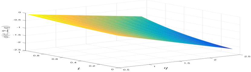
(b) The FIPDE scheme

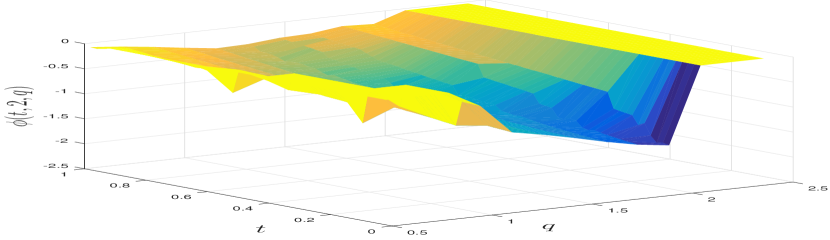
(c) The EMReg scheme

Figure 1: Feedback controls of the LQ optimal liquidation problem with $Q_{0}\sim\mathcal{U}(1,2)$ obtained by using different methods.

We proceed to investigate the robustness of feedback controls obtained by the FIPDE scheme and the EMReg scheme with respect to perturbation of the random initial condition $Q_{0}$, which models the initial inventories of all market participants. As it is practically difficult to obtain the precise distribution of $Q_{0}$, it is desirable for the feedback control to be stable in terms of the uncertainty in the initial law (see, e.g., [28]). In particular, we first obtain approximate feedback controls by applying the FIPDE and EMReg schemes to solve (5.1) with $Q^{\textrm{pre}}_{0}\sim\mathcal{U}(1,2)$, and then examine the performance of these feedback controls on perturbed models with $Q_{0}\sim\mathcal{U}(Q_{0,\min},Q_{0,\max})$ for $Q_{0,\min}\in[0.5,1.5]$ and $Q_{0,\max}\in[1.5,2.5]$.

Figure 2 illustrates the performance of these precomputed controls on models with different $Q_{0}$ in terms of the absolute performance gap $|J(\phi^{\textrm{pre}})-J^{\star}|$, where $J(\phi^{\textrm{pre}})$ is the expected cost of a precomputed feedback control $\phi^{\textrm{pre}}$ on the perturbed model, and $J^{\star}$ is the optimal cost of the perturbed model. One can clearly observe from Figure 2 (left) that the precomputed feedback control from the FIPDE scheme is very robust with respect to perturbation of $Q_{0}$, as it yields extremely small performance gaps for all perturbed models. Moreover, the absolute performance gaps remain almost constants for different $Q_{0}$ with the same expectation. This is because the feedback control from the FIPDE scheme captures the precise spatial dependence of the optimal feedback control of a perturbed problem (i.e., the function $\phi^{\star}$ in (5.4)), while it keeps the measure dependence the same as that for the unperturbed model. As the optimal feedback control of the LQ MFC problem (5.1) depends on the law of $Q_{0}$ only through its first moment, the absolute performance gap $|J(\phi^{\textrm{pre}})-J^{\star}|$ for the FIPDE scheme is purely determined by the perturbation of ${\mathbb{E}}[Q_{0}]$.

In contrast, as shown in Figure 2 (right), the approximate feedback control from the EMReg scheme is very sensitive to perturbations of $Q_{0}$, where absolute performance gaps are typically a few magnitudes larger than those of the FIPDE scheme. This phenomenon is more pronounced if the support of the perturbed $Q_{0}$ is not contained by the interval $[1,2]$, i.e., the support of the original $Q_{0}$. This is because the EMReg scheme (and other pure data-driven algorithms) computes approximate feedback controls merely based on trajectories of the original state process, and consequently the resulting feedback control performs poorly along the trajectories outside the support of the original system. In particular, since it is critical to execute a proper strategy for large values of $Q_{t}$ in the present liquidation problem, a slight perturbation of $Q_{0,\max}$ will significantly worsen the performance of the precomputed control.

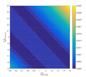
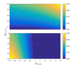
Figure 2: Absolute performance gaps of precomputed feedback controls from the FIPDE scheme (left) and the EMReg scheme (right) on perturbed models with $Q_{0}\sim\mathcal{U}(Q_{0,\min},Q_{0,\max})$.

The improved robustness of the FIPDE scheme over the EMReg scheme can be better analysed by the relative performance gaps $|J(\phi^{\textrm{pre}})-J^{\star}|/|J^{\star}|$, whose distributions (with fixed $Q_{0,\min}$ and varying $Q_{0,\max}$) are summarized by the box plots in Figure 3. We can clearly see that the precomputed control of the FIPDE scheme achieves a relative error of less than 2% on most perturbed models (Figure 2 (left)), while the precomputed control of the EMReg scheme will typically lead to a relative error ranging from $20\%$ to $10^{3}\,\%$ (Figure 3 (top-right)).

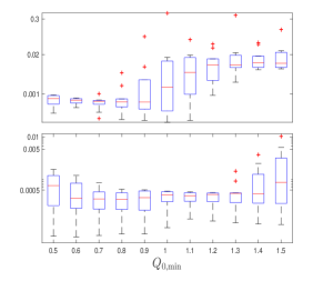
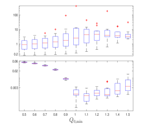
Figure 3: Relative performance gaps of precomputed feedback controls on perturbed models with $Q_{0}\sim\mathcal{U}(Q_{0,\min},Q_{0,\max})$; from left to right: results for the FIPDE and EMReg scheme; from top to bottom: distributions of relative errors for fixed $Q_{0,\min}$ and varying $Q_{0,\max}\in[2,2.5]$ and $Q_{0,\max}\in[1.5,2]$, where on each box, the central line is the median, the edges of the box are the 25th and 75th percentiles, the whiskers extend to non-outliers extreme data points, and outliers are plotted individually.

Finally, we examine the performance of the FIPDE scheme for solving the nonsmooth MFC problem (5.1) with $k_{1}=k_{2}=1$ in (5.1). We initialize Algorithm 1 with $\tau=1/6$ and $\phi^{0}=0$, and for each NAG iteration, discretize the PDE system (5.2) by using the same monotone scheme as that for the LQ case. Note that for all $\tau>0$, the proximal operator of $\tau|\cdot|$ is given by $\text{prox}_{\tau|\cdot|}(x)=\textrm{sgn}(x)(|x|-k_{2}\tau)$ for all $|x|\geq k_{2}\tau$ and $\text{prox}_{\tau\ell}(x)=0$ for all $|x|\leq k_{2}\tau$.

We carry out the FIPDE scheme with 20 NAG iterations, whose convergence is shown in Figure 11 in Appendix A.1; note that in fact 4 NAG iterations are sufficient to approximate the value function accurately. The resulting approximate feedback control is independent of the variable $s$ but nonlinear in the variable $q$. Figure 4 (left) presents the approximate feedback controls for $s=2$ and $(t,q)\in[0,1]\times[0.5,2.5]$, which clearly shows that the nonsmooth cost enhances the sparsity of the optimal strategy, especially near the terminal time. We then analyze the robustness of the FIPDE scheme by exercising the feedback control $\phi^{\textrm{pre}}$ computed with $Q_{0}\sim\mathcal{U}(1,2)$ on perturbed models with $Q_{0}\sim\mathcal{U}(Q_{0,\min},Q_{0,\max})$. Due to the absence of analytic solution for the nonsmooth MFC problem, we compare the expected cost $J(\phi^{\textrm{pre}})$ of $\phi^{\textrm{pre}}$ on the perturbed model against the numerical approximation $J(\phi^{\textrm{pert}})$ of the optimal cost of the perturbed model, where $\phi^{\textrm{pert}}$ is the feedback control obtained by the FIPDE scheme with the perturbed $Q_{0}$. Figure 4 (right) depicts the absolute performance gaps $|J(\phi^{\textrm{pre}})-J(\phi^{\textrm{pert}})|$ for different $Q_{0}$. Due to the nonsmooth cost function, the optimal feedback controls of (5.1) depend nonlinearly on the law of $Q_{0}$, and hence the performance gaps are no longer constant along the diagonals (cf., Figure 2 (left)). However, the absolute performance gaps remain small for all perturbations, which demonstrates the robustness of the FIPDE scheme in the present nonsmooth setting.

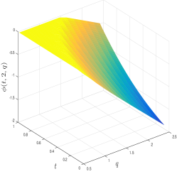
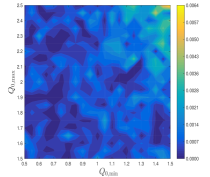
Figure 4: Numerical results of the FIPDE scheme for the nonsmooth optimal liquidation problem with $k_{2}=1$; from left to right: approximate feedback control for $Q_{0}\sim\mathcal{U}(1,2)$, and absolute performance gaps of the precomputed feedback control on perturbed models with $Q_{0}\sim\mathcal{U}(Q_{0,\min},Q_{0,\max})$.

5.2 Sparse consensus control of stochastic Cucker-Smale models

In this section, we study optimal control of the multidimensional stochastic mean-field Cucker-Smale (C-S) dynamics (see, e.g., [43] and [21, Chapter 4]), where the controller aims to enforce consensus emergence of an interactive particle system via (possibly sparse) external intervention. In its general form this leads to a nonsmooth nonconvex MFC problem.

Given a terminal time $T>0$ and a $d$-dimensional adapted control strategy $(\alpha_{t})_{t\in[0,T]}$, we consider the following $2d$-dimensional controlled dynamics with additive noise, which can be viewed as the large population limit of the finite-particle model studied in [25]: for all $t\in[0,T]$,

$$\,\text{\rm{d}}x_{t}=v_{t}\,\,\text{\rm{d}}t,\quad\,\text{\rm{d}}v_{t}=\bigg{(}\int_{\mathbb{R}^{d}\times\mathbb{R}^{d}}\kappa(x_{t},v_{t},x^{\prime},v^{\prime})\,\mathcal{L}_{(x_{t},v_{t})}(\,\text{\rm{d}}x^{\prime},\,\text{\rm{d}}v^{\prime})+\alpha_{t}\bigg{)}\,\,\text{\rm{d}}t+\sigma\,\,\text{\rm{d}}W_{t},$$ (5.5)

with initial state $(x_{0},v_{0})\in L^{2}(\Omega;\mathbb{R}^{d}\times\mathbb{R}^{d})$, where $W$ is a $d$-dimensional Brownian motion defined on a filtered probability space $(\Omega,\mathcal{F},\{\mathcal{F}_{t}\}_{t\in[0,T]},\mathbb{P})$, $\sigma\in\mathbb{R}^{d\times d}$ and $\kappa:\mathbb{R}^{d}\times\mathbb{R}^{d}\times\mathbb{R}^{d}\times\mathbb{R}^{d}\to\mathbb{R}^{d}$ is given by

$$\kappa(x,v,x^{\prime},v^{\prime})=\frac{K(v^{\prime}-v)}{(1+|x-x^{\prime}|^{2})^{\beta}},\quad\textnormal{with some $\beta,K\geq 0$.}$$

It is well-known that for uncontrolled deterministic models (with $\sigma=0$ and $\alpha\equiv 0$), a time-asymptotic flocking behaviour (i.e., all trajectories of the velocity process tend to the same value as $t\to\infty$) only appears for $\beta\leq 1/2$ or for specific initial conditions if $\beta>1/2$; see [25, 24, 9] and references therein. Moreover, as shown in [25, 43], even when the deterministic counterpart exhibits a time-asymptotic flocking behaviour, the additive noise may prevent the emergence of flocking in the stochastic model.

The aim of the controller is to either induce consensus on models that would otherwise diverge, or to accelerate the flocking for an initial configuration that would naturally self-organise. More precisely, for given constants $\gamma_{1},\gamma_{2}\geq 0$, we consider minimizing the following cost functional

$$J(\alpha;(x_{0},v_{0}))=\mathbb{E}\left[\int_{0}^{T}\Big{(}|v_{t}-\mathbb{E}[v_{t}]|^{2}+\gamma_{1}|\alpha_{t}|^{2}+\gamma_{2}|\alpha_{t}|_{1}\Big{)}\,\mathrm{d}t+|v_{T}-\mathbb{E}[v_{T}]|^{2}\right]$$ (5.6)

over all adapted control processes $\alpha$ taking values in $\mathbb{R}^{d}$, where $|\cdot|_{1}$ is the $\ell_{1}$-norm of a given vector. Note that in general, the cost functional $J$ is neither convex nor smooth in the control process $\alpha$, due to the nonlinear interaction kernel $\kappa$ in (5.5) and the $\ell_{1}$-norm in (5.6). However, in the special case with $\beta=\gamma_{2}=0$ and $\gamma_{1}>0$, (5.5)-(5.6) is a LQ MFC problem whose optimal feedback control can be found via Riccati equations (see, e.g., [54, 12]).

In the subsequent two sections, we demonstrate the effectiveness of the FIPDE method (i.e., Algorithm 1) to solve (5.5)-(5.6) with different choices of $\beta,d$ and $\gamma_{2}$. For the $m$-th NAG iteration, given the approximate feedback control $\psi^{m}:[0,T]\times\mathbb{R}^{d}\times\mathbb{R}^{d}\to\mathbb{R}^{d}$ with associated state processes $(x^{m}_{t},v^{m}_{t})_{t\in[0,T]}$, the FIPDE method seeks functions ${u}_{1},{u}_{2}:[0,T]\times\mathbb{R}^{d}\times\mathbb{R}^{d}\to\mathbb{R}^{d}$ satisfying the following coupled system of $2d$-dimensional parabolic PDEs: for all $(t,x,v)\in[0,T]\times\mathbb{R}^{d}\times\mathbb{R}^{d}$,

$$(\partial_{t}u_{1}+\mathscr{L}^{m}u_{1})(t,x,v) =-f^{m}_{1}(t,x,v,u_{2}), \quad{u}_{1}(T,x,v)=0,$$ (5.7a)

$$(\partial_{t}u_{2}+\mathscr{L}^{m}u_{2})(t,x,v) =-f^{m}_{2}(t,x,v,u_{1},u_{2}), \quad{u}_{2}(T,x,v)=2(v-\mathbb{E}[v^{m}_{T}]),$$ (5.7b)

with the operator $\mathscr{L}^{m}$ and the source terms $f^{m}_{1},f^{m}_{2}$ satisfying for all $\varphi\in C^{1,2}([0,T]\times\mathbb{R}^{2d};\mathbb{R})$,

$$\begin{split}(\mathscr{L}^{m}\varphi)(t,x,v)&=\tfrac{1}{2}\textnormal{tr}\big{(}\sigma\sigma^{\mathsf{T}}(\partial_{vv}\varphi)(t,x,v)\big{)}+v^{\mathsf{T}}(\partial_{x}\varphi)(t,x,v)\\ &\quad+\big{(}{{\mathbb{E}}}[\kappa(x,v,{x}^{m}_{t},{v}^{m}_{t})]+\psi^{m}(t,x,v)\big{)}^{\mathsf{T}}(\partial_{v}\varphi)(t,x,v),\\ f^{m}_{1}(t,x,v,u_{2})&={{\mathbb{E}}}[(\partial_{x}\kappa)(x,v,{x}^{m}_{t},{v}^{m}_{t})]u_{2}(t,x,v)+{{\mathbb{E}}}[(\partial_{{x}^{\prime}}\kappa)({x}^{m}_{t},{v}^{m}_{t},{x},{v})u_{2}(t,x^{m}_{t},v^{m}_{t})],\\ f^{m}_{2}(t,x,v,u_{1},u_{2})&=u_{1}(t,x,v)+2(v-\mathbb{E}[v^{m}_{t}])+{{\mathbb{E}}}[(\partial_{v}\kappa)(x,v,{x}^{m}_{t},{v}^{m}_{t})]u_{2}(t,x,v)\\ &\quad+{{\mathbb{E}}}[(\partial_{{v}^{\prime}}\kappa)({x}^{m}_{t},{v}^{m}_{t},{x},{v})u_{2}(t,x^{m}_{t},v^{m}_{t})],\end{split}$$ (5.8)

where for each $w\in\{x,x^{\prime},v,v^{\prime}\}$, $\partial_{w}\kappa$ denotes the Jacobian matrix such that $(\partial_{w}\kappa)_{ij}={\partial_{w_{i}}\kappa_{j}}$. In practice, we approximate the expectations in the coefficients of (5.8) by the corresponding empirical averages over particle approximations of $(x^{m},v^{m})$, which are generated by (2.16) with sufficiently large $N,M\in\mathbb{N}$. The PDE systems with approximated coefficients will be solved by using the finite difference approximation in Section 3 or the residual approximation method in Section 4, depending on the problem dimension $2d$; see Sections 5.2.1 and 5.2.2, respectively, for more details.

We shall also compare the FIPDE method with the neural network-based policy gradient (NNPG) method, which is a pure data-driven algorithm proposed in [22] to solve MFC problems. The NNPG method considers minimizing (5.6) over a class of feedback controls represented by multilayer neural networks with weights $\theta$, and obtains the optimal weights by applying gradient descent algorithms based on simulated trajectories of the state process (5.5) (see Sections 5.2.1 and 5.2.2 for more details). As we shall see soon, the proposed FIPDE method achieves more accurate and interpretable feedback controls than the NNPG method, in both the low-dimensional and high-dimensional settings.

5.2.1 Consensus control of two-dimensional C-S models

This section studies (5.5)-(5.6) for two-dimensional C-S models with different communication rates $\beta$. In particular, we shall perform experiments with the following model parameters: $T=d=K=1$, $\sigma=\gamma_{1}=0.1$, $\gamma_{2}=0$, $\beta\in\{0,10\}$, and $(x_{0},v_{0})$ follows the two-component Gaussian mixture distribution with mixture weights $(0.5,0.5)$, mean $(1.2,1.8)$ and covariance $0.01\mathbb{I}_{2}$ for component 1, and mean $(1.8,1.2)$ and covariance $0.01\mathbb{I}_{2}$ for component 2, where $\mathbb{I}_{2}$ is the $2\times 2$ identity matrix.

We now discuss the implementation details of the FIPDE algorithm with finite difference approximation for the present two-dimensional setting. The FIPDE algorithm is initialized with $\tau=1/6$ and $\phi^{0}\equiv 0$. At the $m$-th NAG iteration, given an approximate feedback control $\psi^{m}$, we first generate particle approximations $(x^{m,l},v^{m,l})_{l=1,\ldots,10^{4}}$ of the state process $(x^{m},v^{m})$ with time stepsize $\Delta t=1/50$ (i.e., (2.16) with $N=10^{4}$ and $M=50$), and replace the expectations in (5.8) by the empirical averages over particles. The PDE system with approximate coefficients is then localized on the domain $\mathcal{D}=[0,5]\times[0,4]$ with boundary conditions being the terminal values, i.e., $(u_{1}(t,x,v),u_{2}(t,x,v))=(0,2(v-\tfrac{1}{N}\sum_{l=1}^{N}v^{m,l}_{T}))$ for all $(t,x,v)\in[0,T]\times\partial\mathcal{D}$. We further construct a semi-implicit first-order monotone scheme (3.6) for the localized system (5.7) by adopting the time stepsize $\Delta t=1/50$ and mesh sizes $h_{x}=5/50$, $h_{v}=4/50$, and discretizing the first-order derivatives in (5.8) via the upwind finite difference and the second-order derivative in (5.8) via the central difference.

For the LQ MFC problem (5.5)-(5.6) with $\beta=0$, we compare the approximate feedback control from the FIPDE scheme with the optimal feedback control given by

$$\phi^{\star}(t,x,v)=-\tfrac{a_{t}}{2\gamma_{1}}(v-{\mathbb{E}}[v^{\star}_{t}]),\quad(t,x,v)\in[0,T]\times{\mathbb{R}}\times{\mathbb{R}},$$ (5.9)

where $a:[0,T]\times{\mathbb{R}}$ satisfies $a^{\prime}_{t}-2Ka_{t}-\frac{1}{2\gamma_{1}}a_{t}^{2}+2=0$ with $a_{T}=2$, and $v^{\star}$ is the optimal velocity process (see, e.g., [54, 12]). The blue line in Figure 5 (left) presents the expected costs of the approximate feedback controls obtained by the FIPDE method at all NAG iterations, which converge exponentially to the optimal cost in terms of the number of NAG iterations; a linear regression of the data shows the absolute error for the $m$-th iteration is of the magnitude $\mathcal{O}(0.55^{m})$. The FIPDE method is benchmarked against the iterative PDE-based (IPDE) algorithm obtained by omitting the momentum step in Algorithm 1 (i.e., $\psi^{m}=\phi^{m}$ for all $m$), whose convergence is shown by the red line in Figure 5 (left). Note that the FIPDE and IPDE methods take a similar time to perform one gradient descent iteration, but the FIPDE method requires much fewer iterations to achieve high accuracy. This shows that the momentum step indeed accelerates the algorithm convergence, and justifies the terminology “fast” in FIPDE. We further depict the approximate feedback control $\phi$ (generated by the last NAG iteration) with $t=0$ and $(x,v)\in[1,2]^{2}$ in Figure 5 (right), which approximates the optimal feedback control $\phi^{\star}(0,\cdot,\cdot)$ (see (5.9)) with a relative error of $1.7\%$ in the $L^{2}$-norm. One can clearly observe that the approximate feedback control captures the affine structure of $\phi^{\star}$ in $v$, constant in $x$.

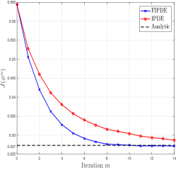
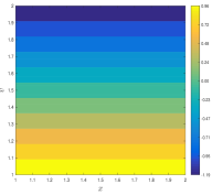
Figure 5: Numerical results of the FIPDE scheme for two-dimensional C-S model with $\beta=0$; from left to right: convergence of the FIPDE method in terms of NAG iterations, and the approximate feedback control at $t=0$.

Then we proceed to study the (nonconvex) MFC problem (5.5)-(5.6) with $\beta=10$, where the uncontrolled velocity process does not exhibit a flocking behaviour; see Figure 12 in Appendix A.2. In the following, we apply the FIPDE method (with the same discretization parameters as above) to design feedback controls and induce consensus for such models. We shall further benchmark the performance of the FIPDE method against a neural network-based policy gradient (NNPG) method (see Algorithm 1 in [22]), whose implementation details are given in Appendix A.2. In particular, we seek an approximate feedback control among a family of neural networks whose flexibility is sufficient to capture the nonlinearity of the optimal feedback control in $(t,x,v)$, and obtain the optimal neural network approximation by running the Adam algorithm [37] with sufficiently many iterations.

Figure 6 exhibits the approximate feedback controls and the associated costs from the FIPDE and NNPG methods. From Figure 6 (left), we see that despite the nonconvexity of the control problem, the FIPDE method converges exponentially in the value function approximation as the iteration index $m$ tends to infinity, with the absolute error $\mathcal{O}(0.5^{m})$. Compared with the IPDE method, the momentum step in Algorithm 1 accelerates the algorithm’s convergence also in the present nonconvex setting. We refer the reader to Figure 12 in Appendix A.2 for the flocking behaviour of the controlled velocity process obtained by the FIPDE method.

More importantly, the FIPDE method generates a more interpretable approximate feedback control compared to the NNPG method, which helps us understand the mechanism of the optimal control process. Note that for the uncontrolled C-S model (5.5) with $\beta>0$, the interaction kernel $\kappa$ indicates that a particle’s velocity is largely affected by the velocities of particles in the nearest neighborhood. Consequently, for a given particle whose velocity is above the average velocity, the further it is away from the population with small velocity, the less internal attraction exists for the particle’s velocity to the average velocity, and the stronger external intervention is required to induce consensus (and similarly for particle whose velocity is below the average velocity). Such a nonlinear dependence of the optimal feedback control on the variable $x$ is correctly captured by the approximate feedback control $\phi$ of the FIPDE method, whose values at $t=0$ are depicted in Figure 6 (middle). Recall that at $t=0$, the average velocity is $1.5$, and particles with velocity below and above $1.5$ cluster around the points $x=1.8$ and $x=1.2$, respectively. Hence, the absolute magnitude of the function $x\mapsto\phi(0,x,v)$ is minimized near $1.8$ if $v>1.5$ and near $1.2$ if $v<1.5$, which confirms our theoretical understanding of the model. By contrast, the NNPG method produces a less interpretable approximate feedback control with no clear dependence on the variable $x$, as shown in Figure 6 (right).

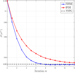
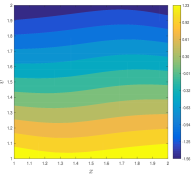
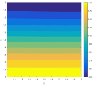
Figure 6: Numerical results of the FIPDE and NNPG methods for two-dimensional C-S model with $\beta=10$; from left to right: convergence of the FIPDE scheme in terms of NAG iterations, the feedback control of the FIPDE method at $t=0$, and the feedback control of the NNPG method at $t=0$.

5.2.2 Sparse consensus control of six-dimensional C-S models

This section examines the performance of the FIPDE method (i.e., Algorithm 1) for solving (5.5)-(5.6) with possibly nonsmooth costs in a six-dimensional setting, where the corresponding PDE systems (5.7) are solved by using the residual approximation approach introduced in Section 4. We carry out numerical experiments with $d=3$, $T=K=1$, $\sigma=0.1\mathbb{I}_{3}$, $\gamma_{1}=0.3$, $(x_{0},v_{0})\sim\mathcal{U}([0,1]^{6})$ (the uniform distribution on $[0,1]^{6}$) but different choices of $\beta,\gamma_{2}\geq 0$. For the sake of presentation, we shall only specify the neural network architectures used in our computation, and refer the reader to Appendix A.2 for the detailed implementation of the empirical risk minimization problem (4.5).

Let us start with the LQ MFC problem by choosing $\beta=\gamma_{2}=0$. We initialize Algorithm 1 with $\phi^{0}=0$ and $\tau=1/5$, and adopt feedforward neural networks with the same architecture to approximate each component of $\phi^{m},\psi^{m}:[0,T]\times{\mathbb{R}}^{6}\to{\mathbb{R}}^{3}$ and $u^{m}:[0,T]\times{\mathbb{R}}^{6}\to{\mathbb{R}}^{6}$ for all NAG iterations. More precisely, for each $m$, we have $\phi^{m}=(\phi^{\theta}_{1},\ldots\phi^{\theta}_{3})$, $\psi^{m}=(\psi^{\theta}_{1},\ldots\psi^{\theta}_{3})$ and $u^{m}=(u^{\theta}_{1},\ldots u^{\theta}_{6})$, where $\phi^{\theta}_{i},\psi^{\theta}_{i},u^{\theta}_{i}$ are some fully-connected networks with the sigmoid activation function, depth 2 (1 hidden layer), and the dimensions of the input, output and hidden layers being 7, 1 and 20, respectively. We then apply the residual approximation method to solve (5.7) on the spatial domain $\mathcal{D}=[-1,2]^{6}$. Note that approximating each component of the solutions individually allows us to capture the heterogeneity among components with shallow networks, and consequently makes the empirical residuals relatively easy to optimize. Moreover, we set $\bar{u}=0$ on $[0,T]\times\mathcal{D}$ for the decomposition (4.2), since in the present LQ case, there is no obvious candidate solution to (5.7), except the exact solution based on Riccati equations.

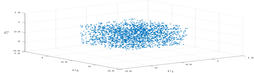
(a) Uncontrolled velocity, $t=0$

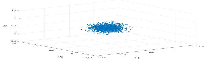
(b) Uncontrolled velocity, $t=1$

(c) Controlled velocity, $t=1$

Figure 13: Uncontrolled and controlled six-dimensional C-S models with $\beta=0$ at different times.

We carry out the FIPDE method with 15 NAG iterations and summarize the numerical results in Table 1. It is clear that the approximate controls and their associated costs of the FIPDE method converge rapidly to the optimal control process and the optimal cost function obtained by Riccati equations. Moreover, a sensitivity analysis of the neural network architectures indicates that the convergence of the FIPDE method is very robust with respect to the network depth $L$, the dimension $H$ of hidden layers, and the (smooth) activation functions. Figure 13 in Appendix A.2 depicts the trajectories of the uncontrolled and controlled velocity processes, which demonstrates that the approximate feedback control of the FIPDE method effectively accelerates the emergence of the flocking behaviour.

Table 1: Impact of the network architecture on the convergence of the FIPDE method. Shown are: (a) the absolute error $|J(\phi^{m})-J^{\star}|$ of the numerical value function $J(\phi^{m})$, and (b) the absolute error $(\mathbb{E}[\sup_{t\in[0,T]}|\alpha_{t}^{m}-\alpha_{t}^{\star}|^{2}])^{\frac{1}{2}}$ of the numerical control process $\alpha^{m}$.

	NAG Itr $m$	1	3	6	9	12	15
$L=2$, $H=20$, $\varrho=\textrm{sigm}$	(a)	0.0401	0.0121	0.0050	0.0023	0.0010	0.0007
	(b)	0.2650	0.1549	0.1015	0.0632	0.0400	0.0283
$L=4$, $H=20$, $\varrho=\textrm{sigm}$	(a)	0.0396	0.0122	0.0045	0.0019	0.0008	0.0005
	(b)	0.2676	0.1667	0.1082	0.0721	0.0470	0.0346
$L=2$, $H=40$, $\varrho=\textrm{sigm}$	(a)	0.0395	0.0127	0.0053	0.0024	0.0012	0.0009
	(b)	0.2638	0.1594	0.1015	0.0663	0.0412	0.0300
$L=2$, $H=20$, $\varrho=\tanh$	(a)	0.0412	0.0197	0.0086	0.0041	0.0022	0.0013
	(b)	0.2659	0.1936	0.1261	0.0860	0.0557	0.0346

We then examine the accuracy of the FIPDE method for approximating the optimal feedback control $\phi^{\star}$, which satisfies $\phi^{\star}(t,x,v)=A_{t}(v-{\mathbb{E}}[v^{\star}_{t}])$ for all $(t,x,v)\in[0,T]\times{\mathbb{R}}^{3}\times{\mathbb{R}}^{3}$, with $A\in C([0,T];{\mathbb{R}}^{3\times 3})$ being the solution to a differential Riccati equation, and $v^{\star}$ being the optimal velocity process. As shown in Figure 7 (left), although the FIPDE method is implemented with feedforward neural networks taking inputs $(t,x,v)$, the resulting approximate feedback control correctly captures the important structures of the optimal control $\phi^{\star}$, i.e., the affineness in $v$ and the independence of $x$. To further highlight the advantage of the PDE-based solver over pure data-driven approaches, we implement the NNPG method with the same neural network architecture (see Appendix A.2 for more details), and compare the resulting feedback control against the FIPDE method and the analytic solution. Comparing Figure 7 (middle) and (right), we see the FIPDE method recovers the exact feedback control accurately on (cross-sections of) the entire space-time domain, while the NNPG method only approximates the exact control on certain sub-domains (depending on the trajectories of the optimal state process), and fails to capture the time dependence of the exact control.

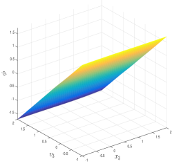
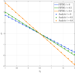
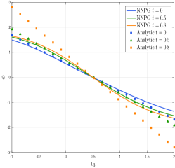
Figure 7: Feedback controls for six-dimensional C-S model with $\beta=\gamma_{2}=0$; from left to right: feedback control of the FIPDE scheme at $t=0$ and different $(x_{3},v_{3})$, feedback controls of the FIPDE scheme and the analytic solution at different $(t,v_{3})$, and feedback controls of the NNPG scheme and the analytic solution at different $(t,v_{3})$, where the remaining components are set to $0.5$.

Now we proceed to apply the FIPDE method to the nonsmooth MFC problem (5.5)-(5.6) with $\beta=0$ and $\gamma_{2}\in\{0.1,0.3\}$. As initial feedback control $\phi^{0}$ for Algorithm 1 we use the approximate feedback control for the LQ problem (with $\gamma_{2}=0$) obtained by the FIPDE method, and choose the stepsize $\tau=1/5$. At the $m$-th NAG iteration, the residual approximation (RA) approach in Section 4 is implemented to solve (5.7) on the domain $\mathcal{D}=[-1,2]^{6}$. In particular, we decompose the numerical solution into the form $\bar{u}+\tilde{u}^{m}$, where $\bar{u}:[0,T]\times{\mathbb{R}}^{6}\to{\mathbb{R}}^{6}$ is the approximate decoupling field of the above LQ problem obtained by the FIPDE method, and $\tilde{u}^{m}:[0,T]\times{\mathbb{R}}^{6}\to{\mathbb{R}}^{6}$ is an unknown nonlinear residual correction. We then approximate the components of $\tilde{u}^{m}$ by neural networks with the sigmoid activation function, depth 4 (3 hidden layers), and the dimensions of the input, output and hidden layers being 7, 1 and 40, respectively, and determine the optimal neural network representation by minimizing the empirical loss (4.5) with 100 SGD iterations (see Appendix A.2). In the following, we refer to the method as “RA with 100 SGD”.

To demonstrate the efficiency of the RA approach, we compare the performance of the above FIPDE method to those of the Direct Method and the NNPG method. In the Direct Method, we do not decompose numerical solutions in a separable form (i.e., we set $\bar{u}=0$ in (4.2)), and directly minimize the residuals of (5.7) over neural networks. For each NAG iteration, we choose the same trial functions (4-layer networks with hidden width 40), numbers of training samples and learning rates of the SGD algorithm as those of the FIPDE method, and perform $q$ SGD iterations with different choices of $q\in\mathbb{N}$, which will be referred to as “DM with $q$ SGD” in the following discussion. In the NNPG method, we minimize the objective (5.6) over all feedback controls parametrized by 4-layer networks with the same architecture (see Appendix A.2 for more details).

Figure 8 depicts the convergence of value functions from “RA with 100 SGD” and “DM with $q$ SGD” (with $q\in\{200,500,1000\}$) for solving (5.5)-(5.6) with $\gamma_{2}=0.1$, where we take the value function from the NNPG method as a reference value. It clearly demonstrates that the residual approximation requires significantly less number of SGD iterations than the Direct Method for solving the PDE system (5.7) at each NAG iteration; in particular, the approximate feedback controls of “RA with 100 SGD” (the red line) at all NAG iterations consistently achieve lower costs than those of “DM with $1000$ SGD” (the blue line). Observe that for each NAG iteration, the computation times of the residual approximation approach and the Direct Method scale linearly with the number of SGD iterations. Thus the residual decomposition (4.2) reduces the total computational time of the Direct Method by roughly a factor of 10. A similar efficiency enhancement of the residual approximation approach has also been observed in the nonsmooth problem (5.5)-(5.6) with $\beta=0$ and $\gamma_{2}=0.3$.

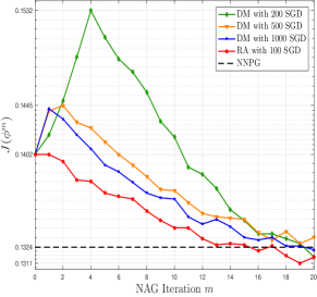
Figure 8: Efficiency improvement of the residual approximation approach over the Direct Method for six-dimensional C-S model with $\beta=0$ and $\gamma_{2}=0.1$.

Figure 9 presents the approximate feedback controls of the nonsmooth problem (5.5)-(5.6) with different $\gamma_{2}>0$, obtained by using the FIPDE and NNPG methods. Due to the $\ell_{1}$-norm in (5.6), the optimal feedback control is nonlinear in $v$ and admits a sparse structure. That is, the optimal decision is to act only on the particles whose velocities are far from the mean and to steer them to consensus, without intervening with the particles near the consensus manifold [20]. As shown in Figure 9 (left) and (middle), the approximate controls of the FIPDE method correctly capture the sparse features of the optimal control, where the zero-control region shrinks as the terminal time approaches and expands as the parameter $\gamma_{2}$ increases. On the other hand, the NNPG method results in a (suboptimal) non-sparse linear strategy, which suggests to control all agents with mild strength. It also fails to capture the time dependence of the optimal control, as already observed in the LQ setting (see Figure 7). Consequently, for $\gamma_{2}=0.3$, the control of the NNPG method has a $2.4\%$ higher expected cost (5.6) than that of the FIPDE method (in terms of the relative error); the expected costs for the NNPG and FIPDE methods are 0.1635 and 0.1596, respectively.

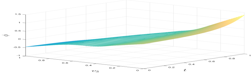
(a) FIPDE for $\gamma_{2}=0.1$

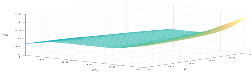
(b) FIPDE for $\gamma_{2}=0.3$

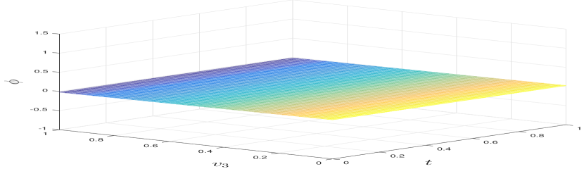
(c) NNPG for $\gamma_{2}=0.3$

Figure 9: Feedback controls for six-dimensional C-S models with $\beta=0$ and $\gamma_{2}>0$, where the controls are evaluated at different $(t,v_{3})$ with the remaining components being $0.5$.

Finally, we apply the FIPDE method to solve the nonconvex MFC problem (5.5)-(5.6) with $\beta=1$ and $\gamma_{2}=0$. As in the two-dimensional setting studied in Section 5.2.1, the uncontrolled velocity process does not form a consensus, and the optimal feedback control in general depends nonlinearly on $(t,x,v)$. Similar to the above nonsmooth problem, we use the LQ feedback control as the initial guess $\phi^{0}$ in Algorithm 1, choose the stepsize $\tau=1/5$, and employ the residual approximation approach to solve (5.7) at all NAG iterations, with the candidate solution $\bar{u}$ being the approximate decoupling field of the LQ problem. The components of the residual $\tilde{u}^{m}$ and the controls $\phi^{m},\psi^{m}$ are approximated by $7$-layer neural networks with hidden width 60 (see Appendix A.2 for more details). Figure 10 compares the uncontrolled velocity process and the controlled velocity process obtained by the FIPDE method (with $6$ NAG iterations), which clearly demonstrates the effectiveness of the FIPDE method on inducing consensus. Compared with the NNPG method (implemented with the same neural networks), the FIPDE method results in a similar value function but a better consensus at the terminal time; the value functions of the FIPDE and NNPG methods are 0.111 and 0.114, respectively, while the final variances ${\mathbb{E}}[|v_{T}-{\mathbb{E}}[v_{T}]|^{2}]$ obtained by the FIPDE and NNPG methods are 0.007 and 0.01, respectively. Moreover, similar to the above examples in Figures 7 and 9, the FIPDE method captures the nonlinear time dependence of the optimal control, while the NNPG method leads to an approximate control that is constant in $t$ (plots omitted).

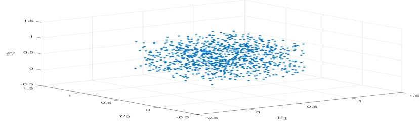
(a) Uncontrolled velocity, $t=0$

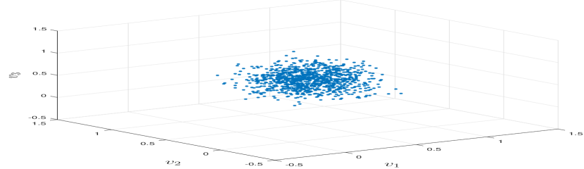
(b) Uncontrolled velocity, $t=1$

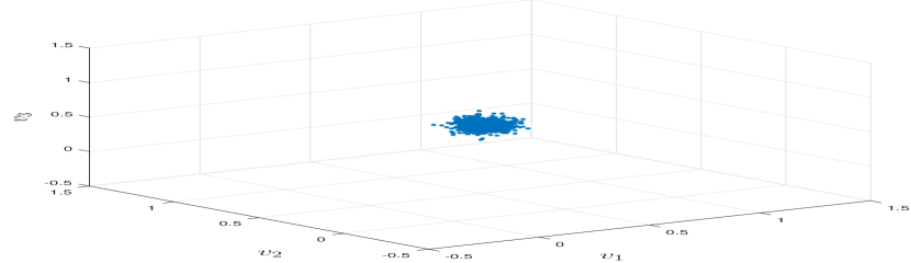
(c) Controlled velocity, $t=1$

Figure 10: Uncontrolled and controlled six-dimensional C-S models with $\beta=1$ at different times.

Appendix A Supplementary materials for Section 5

A.1 Supplementary materials for Section 5.1

Convergence of the NAG iteration.

Figure 11 presents the expected costs of the approximate feedback controls obtained by all NAG iterations of the FIPDE and EMReg methods for the optimal liquidation problem (5.1) with $Q_{0}\in\mathcal{U}(1,2)$, $k_{1}=1$ and $k_{2}\in\{0,1\}$. To estimate the optimal expected cost for the LQ setting (with $k_{2}=0$), we implement the exact feedback control (5.4) with time stepsize $\Delta t=1/50$, and replace the expectation in (5.1) by the empirical average over $10^{6}$ sample trajectories of the state processes. It shows that for both the LQ and nonsmooth MFC problems, the FIPDE and EMReg methods give convergent approximations to the optimal cost functions as the number of NAG iterations tends to infinity. Moreover, a linear regression of the data indicates that the FIPDE method approximates the value function with an absolute error of the magnitude $\mathcal{O}(m^{-2.7})$ for the LQ case.

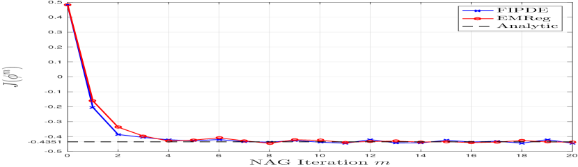
(a) LQ case with $k_{2}=0$

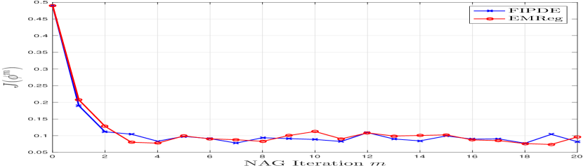
(b) Nonsmooth case with $k_{2}=1$

Figure 11: Convergence of the FIPDE and EMReg methods for approximating the value functions of optimal liquidation problems (5.1) in terms of NAG iteration.

Computational time.

The FIPDE method is implemented by using Matlab R2016b on a laptop with 2.2GHz 4-core Intel Core i7 processor and 16 GB memory. The computation takes around 1 second per NAG iteration. The EMReg method is implemented by using Matlab R2020b on a PC with 2.1GHz 6-core Intel Core i5 processor and 16 GB memory. The computation takes around 5 minutes per NAG iteration based on our implementation.

A.2 Supplementary materials for Section 5.2

Effectiveness of the FIPDE method for two-dimensional models.

Figure 12 compares the uncontrolled two-dimensional C-S model with $\beta=10$ and the controlled model obtained by the FIPDE method, where the scatter plots are generated based on $10^{4}$ simulated trajectories. One can clearly observe that the uncontrolled velocity process does not admit a time-asymptotic flocking behaviour, and the feedback control from the FIPDE method effectively induces the consensus of the velocity process.

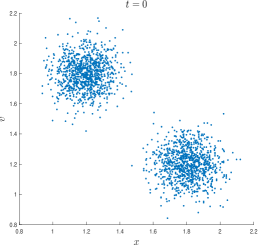
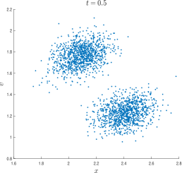
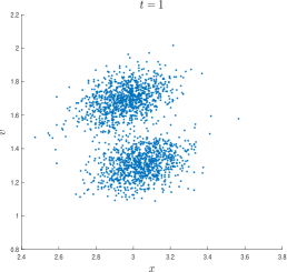
(a) Uncontrolled position and velocity

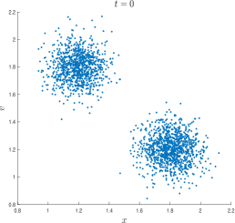
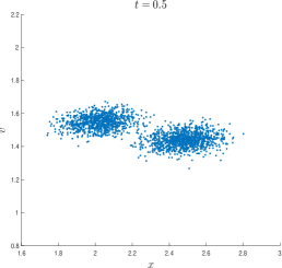
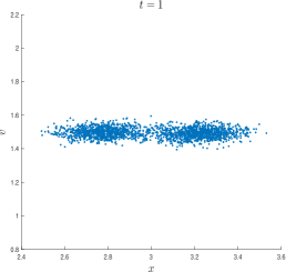
(b) Controlled position and velocity obtained by the FIPDE method

Figure 12: Uncontrolled and controlled two-dimensional C-S models with $\beta=10$ at different times.

Effectiveness of the FIPDE method for six-dimensional models with $\beta=0$.

Figure 12 compares the uncontrolled six-dimensional C-S model with $\beta=0$ and the controlled model obtained by the FIPDE method with quadratic costs (i.e., $\gamma_{2}=0$ in (5.6)), where the scatter plots are generated based on $5\times 10^{3}$ simulated trajectories. One can clearly observe that the feedback control from the FIPDE method accelerates the consensus of the velocity process.

Implementation of the NNPG method for two-dimensional models.

We implement the neural network-based policy gradient (NNPG) method using PyTorch for the optimal control of two-dimensional C-S models with $\beta=10$ as follows. The set of trial functions for feedback controls consists of $7$ layer fully-connected networks with the sigmoid activation function and the dimensions of input, hidden and output layers being equal to $3$, $70$ and $1$, respectively. The optimal weights $\theta$ of the network are obtained by running the Adam algorithm [37] with $5\times 10^{4}$ iterations and a decaying learning rate scheduler. At each iteration, we generate $10^{2}$ trajectories of (5.5) by using (2.16) with time stepsize $\Delta t=0.02$, approximate the functional $J$ in (5.6) by the empirical average of simulated trajectories, and perform gradient descent based on the empirical loss. The learning rate is initialized at $0.0005$ and will be reduced by a factor of 0.3 if the loss does not decrease after 10 iterations. The minimum learning rate is set to be $10^{-6}$.

Implementation of the NNPG method for six-dimensional models.

We state the PyTorch implementation of the NNPG method for six-dimensional C-S models with different choices of $\beta,\gamma_{2}$ used in Section 5.2. As the chosen neural network architecture for each example has been specified in Section 5.2, it remains to discuss the implementation of the Adam algorithm. For $\beta=0$ and $\gamma_{2}\in\{0,0.1,0.3\}$, at each SGD iteration, we generate $10^{3}$ trajectories of (5.5) by using (2.16) with time stepsize $\Delta t=0.02$, and perform gradient descent based on an empirical approximation of $J$ in (5.6). We choose the same “reduce on plateau” learning rate scheduler as the above two-dimensional case and perform a sufficiently large number of iterations until the empirical loss stabilizes. For $\beta=1$ and $\gamma_{2}=0$, we reduce the number of simulated trajectories per iteration to $10^{2}$ and keep the remaining configurations. This helps to accommodate the increasing computational cost of simulating (5.5) with $\beta>0$.

Implementation of the FIPDE method for six-dimensional models.

We state the PyTorch implementation of the FIPDE method for six-dimensional C-S models with different choices of $\beta,\gamma_{2}$ used in Section 5.2. Before stating the configuration details, we remark that the algorithm’s hyperparameters have not been optimally tuned and hence the following choices may not be the optimal combination. The neural network architectures for all examples have been specified in Section 5.2.

For all NAG iterations, we sample $N$ trajectories of (5.5) by using (2.16) with $\Delta t=0.01$, where $N=4\times 10^{4}$ for $\beta=\gamma_{2}=0$, and $N=5\times 10^{3}$ for the remaining cases. Then, for all choices of $\beta,\gamma_{2}$, we apply the Adam algorithm to solve the corresponding risk minimization problem (4.4) with the initial learning rate 0.005. The learning rate will be decreased by employing the same “reduce on plateau” scheduler as the above NNPG method for the examples with $\beta=0,\gamma_{2}\in\{0,0.1,0.3\}$, while for the example with $\beta=1,\gamma_{2}=0$ it will be decreased by a factor of 0.8 for every 5000 SGD iterations.

At each SGD iteration, a mini-batch of points with size 20 is drawn by following uniform distributions from the interior and boundaries of the domain (i.e., $N_{\textrm{in}}=N_{\textrm{ter}}=N_{\textrm{bdy}}=20$ in (4.5)). Based on these samples, we compute the empirical loss (4.5) with certain $\eta_{1},\eta_{2}>0$ depending on the model parameters. In particular, for $\beta=\gamma_{2}=0$, we choose $\eta_{1}=5$, $\eta_{2}=10$ for the first 6 NAG iterations and $\eta_{1}=2$, $\eta_{2}=5$ for the remaining NAG iterations to balance the interior and boundary losses, while for $\beta=0$, $\gamma_{2}=\{0,1,0.3\}$ and $\beta=1$, $\gamma_{2}=0$, we choose $\eta_{1}=1,\eta_{2}=1/400$ and $\eta_{1}=1,\eta_{2}=1/800$, respectively, across all NAG iterations. The total number of Adam iterations is chosen as 9000 for $\beta=\gamma_{2}=0$, 100 for $\beta=0,\gamma_{2}\in\{0.1,0.3\}$, and 20000 for $\beta=1,\gamma_{2}=0$.

To solve the supervised learning problem (4.6), we carry out the Adam algorithm with initial learning rate 0.001, which will be reduced by employing the same scheduler as that for solving (4.4). We shall randomly draw a mini-batch of points with size 20 at each iteration, and run the algorithm with sufficiently many iterations until the loss stabilizes.

Computational time.

For the two-dimensional C-S models, the FIPDE method is implemented in Matlab R2016b on a laptop with 2.2GHz 4-core Intel Core i7 processor and 16 GB memory. The computation with 15 NAG iterations takes around 30 seconds for $\beta=0$ and around $10$ minutes for $\beta=10$, due to an increased computational cost in evaluating the interaction kernel $\kappa$ for general $\beta>0$. The NNPG method is implemented in Python 3.8.5 on a PC with 2.1GHz 6-core Intel Core i5 processor and 16 GB memory. The computation with $5\times 10^{4}$ Adam iterations takes around 2 hours.

For the six-dimensional C-S models, both the FIPDE and NNPG methods are implemented by using Python 3.8.5 on a PC with 2.1GHz 6-core Intel Core i5 processor and 16 GB memory. The NNPG method typically takes around 20-40 minutes, where the precise computation time depends on the complexity of the problem and the number of SGD iterations used in the simulation. The FIPDE method takes around 20 minutes per NAG iteration for $\beta=0$, and around 8 hours per NAG iteration for $\beta=1$. Note that these times can be shortened if we fine tune the hyperparameters (e.g., the number of SGD iterations) and perform the computation on GPUs.

References

- [1] B. Acciaio, J. Backhoff-Veraguas, and R. Carmona, Extended mean field control problems: stochastic maximum principle and transport perspective, SIAM Journal on Control and Optimization, 57 (2019), pp. 3666–3693.
- [2] Y. Achdou and M. Laurière, On the system of partial differential equations arising in mean field type control, arXiv preprint arXiv:1503.05044, (2015).
- [3] , Mean field type control with congestion (II): An augmented Lagrangian method, Applied Mathematics & Optimization, 74 (2016), pp. 535–578.
- [4] , Mean field games and applications: Numerical aspects, Mean Field Games, (2020), pp. 249–307.
- [5] G. Albi, M. Herty, D. Kalise, and C. Segala, Moment-driven predictive control of mean-field collective dynamics, arXiv preprint arXiv:2101.01970, (2021).
- [6] A. Angiuli, C. V. Graves, H. Li, J.-F. Chassagneux, F. Delarue, and R. Carmona, Cemracs 2017: numerical probabilistic approach to MFG, ESAIM: Proceedings and Surveys, 65 (2019), pp. 84–113.
- [7] R. Archibald, F. Bao, J. Yong, and T. Zhou, An efficient numerical algorithm for solving data driven feedback control problems, Journal of Scientific Computing, 85 (2020), pp. 1–27.
- [8] B. Azmi, D. Kalise, and K. Kunisch, Optimal feedback law recovery by gradient-augmented sparse polynomial regression, Journal of Machine Learning Research, 22 (2021), pp. 1–32.
- [9] R. Bailo, M. Bongini, J. A. Carrillo, and D. Kalise, Optimal consensus control of the Cucker-Smale model, IFAC-PapersOnLine, 51 (2018), pp. 1–6.
- [10] J. Bao, C. Reisinger, P. Ren, and W. Stockinger, First-order convergence of Milstein schemes for McKean–Vlasov equations and interacting particle systems, Proceedings of the Royal Society A, 477 (2021), p. 20200258.
- [11] G. Barles and P. E. Souganidis, Convergence of approximation schemes for fully nonlinear second order equations, Asymptotic Analysis, 4 (1991), pp. 271–283.
- [12] M. Basei and H. Pham, Linear-quadratic McKean–Vlasov stochastic control problems with random coefficients on finite and infinite horizon, and applications, arXiv preprint arXiv:1711.09390, (2017).
- [13] A. Beck, First-order methods in optimization, SIAM, 2017.
- [14] A. Beck and M. Teboulle, Fast gradient-based algorithms for constrained total variation image denoising and deblurring problems, IEEE transactions on image processing, 18 (2009), pp. 2419–2434.
- [15] , A fast iterative shrinkage-thresholding algorithm for linear inverse problems, SIAM Journal on Imaging Sciences, 2 (2009), pp. 183–202.
- [16] C. Bender and J. Zhang, Time discretization and Markovian iteration for coupled FBSDEs, The Annals of Applied Probability, 18 (2008), pp. 143–177.
- [17] A. Bensoussan, J. Frehse, P. Yam, et al., Mean field games and mean field type control theory, vol. 101, Springer, 2013.
- [18] I. H. Biswas, E. R. Jakobsen, and K. H. Karlsen, Difference-quadrature schemes for nonlinear degenerate parabolic integro-PDE, SIAM Journal on Numerical Analysis, 48 (2010), pp. 1110–1135.
- [19] M. Bossy and D. Talay, A stochastic particle method for the McKean–Vlasov and the Burgers equation, Mathematics of Computation, 66 (1997), pp. 157–192.
- [20] M. Caponigro, M. Fornasier, B. Piccoli, and E. Trélat, Sparse stabilization and optimal control of the Cucker-Smale model, Mathematical Control and Related Fields, 3 (2013), pp. 447–466.
- [21] R. Carmona and F. Delarue, Probabilistic Theory of Mean Field Games with Applications I, Springer, 2018.
- [22] R. Carmona and M. Laurière, Convergence analysis of machine learning algorithms for the numerical solution of mean field control and games: II–the finite horizon case, arXiv preprint arXiv:1908.01613, (2019).
- [23] , Convergence analysis of machine learning algorithms for the numerical solution of mean field control and games I:–the ergodic case, SIAM Journal on Numerical Analysis, 59 (2021), pp. 1455–1485.
- [24] J. A. Carrillo, M. Fornasier, J. Rosado, and G. Toscani, Asymptotic flocking dynamics for the kinetic Cucker-Smale model, SIAM Journal on Mathematical Analysis, 42 (2010), pp. 218–236.
- [25] F. Cucker and S. Smale, Emergent behavior in flocks, IEEE Transactions on Automatic Control, 52 (2007), pp. 852–862.
- [26] K. Debrabant and E. Jakobsen, Semi-lagrangian schemes for linear and fully non-linear diffusion equations, Mathematics of Computation, 82 (2013), pp. 1433–1462.
- [27] W. E, J. Han, and A. Jentzen, Deep learning-based numerical methods for high-dimensional parabolic partial differential equations and backward stochastic differential equations, Communications in Mathematics and Statistics, 5 (2017), pp. 349–380.
- [28] M. Germain, M. Laurière, H. Pham, and X. Warin, Deepsets and their derivative networks for solving symmetric PDEs, arXiv preprint arXiv:2103.00838, (2021).
- [29] M. Germain, J. Mikael, and X. Warin, Numerical resolution of McKean–Vlasov FBSDEs using neural networks, arXiv preprint arXiv:1909.12678, (2019).
- [30] S. Ghadimi and G. Lan, Accelerated gradient methods for nonconvex nonlinear and stochastic programming, Mathematical Programming, 156 (2016), pp. 59–99.
- [31] E. Gobet and M. Grangereau, Extended McKean–Vlasov optimal stochastic control applied to smart grid management, (2019).
- [32] O. Guéant, The Financial Mathematics of Market Liquidity: From optimal execution to market making, vol. 33, CRC Press, 2016.
- [33] X. Guo, A. Hu, and Y. Zhang, Reinforcement learning for linear-convex models with jumps via stability analysis of feedback controls, arXiv preprint arXiv:2104.09311, (2021).
- [34] B. Hambly, R. Xu, and H. Yang, Policy gradient methods for the noisy linear quadratic regulator over a finite horizon, SIAM J. Control Optim., 59 (2021), pp. 3359–3391.
- [35] K. Ito, C. Reisinger, and Y. Zhang, A neural network-based policy iteration algorithm with global -superlinear convergence for stochastic games on domains, Foundations of Computational Mathematics, 21 (2021), pp. 331–374.
- [36] B. Kerimkulov, D. Šiška, and L. Szpruch, A modified MSA for stochastic control problems, Applied Mathematics & Optimization, (2021), pp. 1–20.
- [37] D. P. Kingma and J. Ba, Adam: A method for stochastic optimization, arXiv preprint arXiv:1412.6980, (2014).
- [38] H. J. K. Kushner, H. J. Kushner, P. G. Dupuis, and P. Dupuis, Numerical methods for stochastic control problems in continuous time, vol. 24, Springer Science & Business Media, 2001.
- [39] J.-P. Lemor, E. Gobet, and X. Warin, Rate of convergence of an empirical regression method for solving generalized backward stochastic differential equations, Bernoulli, 12 (2006), pp. 889–916.
- [40] H. Li and Z. Lin, Accelerated proximal gradient methods for nonconvex programming, Advances in neural information processing systems, 28 (2015).
- [41] Q. Li, Y. Zhou, Y. Liang, and P. K. Varshney, Convergence analysis of proximal gradient with momentum for nonconvex optimization, in International Conference on Machine Learning, PMLR, 2017, pp. 2111–2119.
- [42] T. Miller, Explanation in artificial intelligence: Insights from the social sciences, Artificial Intelligence, 267 (2019), pp. 1–38.
- [43] M. Nourian, P. E. Caines, and R. P. Malhamé, Mean field analysis of controlled Cucker-Smale type flocking: Linear analysis and perturbation equations, IFAC Proceedings Volumes, 44 (2011), pp. 4471–4476.
- [44] É. Pardoux, Backward stochastic differential equations and viscosity solutions of systems of semilinear parabolic and elliptic PDEs of second order, in Stochastic Analysis and Related Topics VI, Springer, 1998, pp. 79–127.
- [45] L. Pfeiffer, Numerical methods for mean-field-type optimal control problems, arXiv preprint arXiv:1703.10001, (2017).
- [46] H. Pham and X. Wei, Bellman equation and viscosity solutions for mean-field stochastic control problem, ESAIM: Control, Optimisation and Calculus of Variations, 24 (2018), pp. 437–461.
- [47] C. Reisinger, W. Stockinger, and Y. Zhang, Optimal regularity of extended mean field controls and their piecewise constant approximation, arXiv preprint arXiv:2009.08175v2, (2020).
- [48] , A posteriori error estimates for fully coupled McKean–Vlasov forward-backward SDEs, arXiv preprint arXiv:2007.07731, (2020).
- [49] , Linear convergence of a policy gradient method for finite horizon continuous time stochastic control problems, arXiv preprint arXiv:2203.11758, (2022).
- [50] C. Reisinger and Y. Zhang, Rectified deep neural networks overcome the curse of dimensionality for nonsmooth value functions in zero-sum games of nonlinear stiff systems, Analysis and Applications, 18 (2020), pp. 951–999.
- [51] M. Schmidt, N. Roux, and F. Bach, Convergence rates of inexact proximal-gradient methods for convex optimization, Advances in neural information processing systems, 24 (2011).
- [52] J. Sirignano and K. Spiliopoulos, DGM: A deep learning algorithm for solving partial differential equations, Journal of Computational Physics, 375 (2018), pp. 1339–1364.
- [53] D. Šiška and Ł. Szpruch, Gradient flows for regularized stochastic control problems, arXiv preprint arXiv:2006.05956, (2020).
- [54] J. Yong, Linear-quadratic optimal control problems for mean-field stochastic differential equations, SIAM Journal on Control and Optimization, 51 (2013), pp. 2809–2838.