Synchronization of Frequency Modulated Multi-Agent Systems

Abstract

Oscillation synchronization phenomenon is widely observed in natural systems through frequency modulated signals, especially in biological neural networks. Frequency modulation is also one of most widely used technologies in engineering. However, due to the technical difficulty, oscillations are always simplified as unmodulated sinusoidal-like waves in studying the synchronization mechanism in the bulky literature over the decades. It lacks mathematical principles, especially systems and control theories, for frequency modulated multi-agent systems. This paper aims to bring a new formulation of synchronization of frequency modulated multi-agent systems. It develops new tools to solve the synchronization problem by addressing three issues including frequency observation in nonlinear frequency modulated oscillators subject to network influence, frequency consensus via network interaction subject to observation error, and a well placed small gain condition among them. The architecture of the paper consists of a novel problem formulation, rigorous theoretical development, and numerical verification.

I Introduction

Frequency modulated signals extensively exist in natural network systems such as neural circuits. Neuroscientists are interested in modeling nervous systems from simple neural networks to even the human brain. One of the basic areas is to study the neural network models for rhythmic body movements during animal locomotion. Such spinal neural networks are called central pattern generators (CPGs) that, as oscillator circuits, can generate coordinated signals for rhythmic body movements. It has been well understood that “most neurons use action potentials (APs), brief and uniform pulses of electrical activity, to transmit information… the strength at which an innervated muscle is flexed depends solely on the ‘firing rate,’ the average number of APs per unit time (a ‘rate code’)" [1]. In other words, the transmitted signals are frequency modulated. For example, the frequency modulated signals recorded in a real CPG network are shown in Fig. 1 for the dorsal-ventral swimmer Tritonia, a genus of sea slugs.

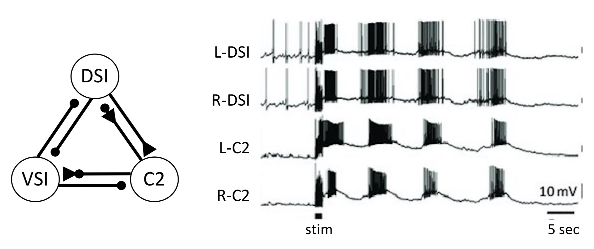
Figure 1: A real frequency modulated CPG model. The neural circuit and swim motor patters for the dorsal-ventral swimmer Tritonia. Left: The Tritonia swim CPG consists of three neuron types: DSI, C2, and VSI. Right: Simultaneous intracellular micro-electrode recordings show that two contralateral DSIs fire bursts of APs in phase with each other and slightly ahead of the two C2s. VSI (not recorded here) fires APs in the inter-burst interval. Courtesy of PNAS [2].

Frequency modulation (FM) is also one of most widely used technologies in engineering. The conventional FM is the encoding of information in a carrier wave by varying the instantaneous frequency of the wave. It has a long history with applications in telecommunications, radio broadcasting, signal processing, and computing [3, 4, 5]. For instance, in radio transmission, FM, compared with an equal power amplitude modulation signal, has the advantage of a larger signal-to-noise ratio and therefore rejects radio frequency interference. Inspired by the aforementioned biological CPGs discovered in animal locomotion, engineers have applied artificial CPGs as oscillator circuits in robotics [6, 7, 8]. Such artificial CPGs can generate frequency modulated signals, resembling the firing bursts of APs, to control robotic locomotion.

However, it lacks mathematical principles, especially systems and control theories, for frequency modulated multi-agent systems. A multi-agent system (MAS) refers to a group of multiple dynamic entities (called agents) that share information or tasks to accomplish a common objective. The agents in an MAS can be circuits, autonomous vehicles, robots, power plants in electrical grid, and other dynamic entities. A CPG network in its dynamic formulation is a typical MAS where each ganglion circuit (group of neurons) is regarded as an agent and they generate patterned signals through inter-agent coordination. In real biological CPGs, the signals of burst firing are frequency modulated [9, 10, 11]. However, the mathematical principles for such CPGs have yet to be studied in terms of their coordinated behaviors. The research was mainly conducted based simplified unmodulated CPG models. For example, the signals of burst firing are approximately represented by unmodulated sinusoidal-like waves when the adaptivity property of CPG circuits was studied for Hirudo verbena, a species of leech. Such an unmodulated leech CPG model was used in [12, 13] (and many other references) to significantly reduce model complexity as there exists no systems and control theory for frequency modulated MASs.

Over the past two decades, abundant researchers have extensively studied MASs and achieved numerous outcomes, across the disciplines of biology, statistical physics, computer sciences, sociology, management sciences, and systems and control engineering. They have established many systems and control theories and engineering tools for various engineering tasks formulated as consensus, rendezvous, swarm, flocking, formation, etc. The early work on control of MASs focused on the so-called consensus problem where a networked set of agents intends to merge to a common state; see, e.g., [14, 15, 16] for simple linear homogenous MASs. A major technical question was to understand the influence of network topology on collaborative behaviors.

The research has been widely extended to deal with more general homogeneous MASs in literature, e.g., [17, 18, 19] for continuous-time systems and [20, 21, 22, 23] for discrete-time systems. This line of research has also quickly spread to many other related problems such as synchronization, formation, flocking, swarming and rendezvous [24, 25, 26]. It is well known that the collective property, in particular, consensus is closely related to the eigenvalue distributions of the so-called Laplacian matrix, which in turn is crucially influenced by the network topology. It is fair to say that the existing control strategies for analysis and control of linear homogeneous MASs are mature using basic Laplacian matrix properties in graph theory.

The mature solutions to various control problems for homogenous MASs rely on the prerequisite that all the agents share share common dynamics. So, they mainly focus on trajectory synchronization. In the recent decade, researchers have put more efforts on synchronization of complicated heterogeneous MASs, where the major challenge arises from the lack of common dynamics. To deal with this challenge, the work in [27, 28] assumes a common virtual exosystem that defines a trajectory on which all agents synchronize to. Researchers also studied the problem using different concepts of homogenization in, e.g., [29, 30]. Some other relevant techniques can be found in [31, 32], etc.

When researchers turned to nonlinear MASs, they first applied the linear techniques to deal with nonlinearities under certain constraints on the growth rates such as a globally Lipschitz-like condition; see, e.g., [33, 34]. The early research on nonlinear collective dynamic behaviors was also found on synchronization of simply coupled nonlinear systems. The complexity is not from network but individual nonlinear characteristics. Typical examples include synchronization of master-slave chaotic systems [35], Kuramoto models [36], and coupled harmonic oscillators [37], etc.

Synchronization of general nonlinear heterogeneous MASs is the state-of-the-art of this field. This problem was studied in [38, 39, 40] using a generalized output regulation framework where the agents converge to various design of specified reference models. In a leader-following setting, the problem was formulated as a cooperative output regulation problem in, e.g., [41] where agents achieve synchronization on a trajectory that is assigned by one or more leaders. When the leader’s system dynamics are unknown to some agents, adaptive schemes were developed in, e.g., [42, 43, 44]. These design approaches for heterogeneous MASs can be illustrated as “reference consensus + agent-reference regulation” where the synchronized behavior is determined by the specified reference model dynamics (called virtual exosystem, exosystem, homogeneous model, internal model, reference model, or leader, etc.) rather than inherent agent dynamics.

On the contrary, to adopt inherent agent dynamics rather than the specified common dynamics, people studied the so-called dynamics consensus/synchronization problem as the prerequisite for trajectory synchronization. For example, the authors of [45, 46] proposed the concept of emergent dynamics which is an “average” of the “units’ drifts”. An MAS reaches dynamic consensus if the agents’ trajectories converge to the one generated by the emergent dynamics. However, synchronization errors exist in these works due to the heterogeneity between unit dynamics and emergent dynamics, which may be diminished by increasing the interconnection gain. The idea was also applied on Andronov-Hopf oscillators [47] and Stuart-Landau oscillators [48]. A more recent result on dynamics synchronization was developed in [49, 50] in a new formulation of autonomous synchronization. The result ensures that both the synchronized agent dynamics and the synchronized states are not specified a priori but autonomously determined by the inherent properties and the initial states of agents.

In all the references discussed in the above survey of MASs, the final target of synchronization is on agent trajectories. It can be achieved either through direct exchange of trajectory information via network (homogeneous MASs) or indirectly through consensus of specified or autonomous reference models plus regulation of agent trajectories to references (heterogeneous MASs). A key stumbling block in generalizing the existing MAS control techniques to frequency modulated MASs is that the techniques require direct or indirect exchange and coordination of unmodulated values of agent trajectories in time domain. However, for frequency modulated MASs, the target is not determined by the instantaneous values of agent trajectories.

The main contribution of this paper is the first attempt to establish a framework for synchronization of frequency modulated MASs. There is rare systems and control theory (analysis or controller synthesis) available for frequency modulated MASs. The technical challenges lie in the fact that the frequency information is hidden from the instantaneous agent values observed or transmitted in a network. Analysis and control of frequency modulated MASs relies on an effective distributed frequency demodulation theory, which is still an open topic. Technically, we will first develop a new method to construct a frequency observer of a nonlinear system, especially subject to an external input representing synchronization error. None of the existing observer design methods is applicable in this scenario. Moreover, the gain from the external input to the observation error should be made arbitrarily small. Secondly, we will design a frequency synchronization approach assuming the frequency observers work with appropriate observation errors. As the two actions occur concurrently, we will also ensure a deliberately formulated small gain condition. The complete framework is established by an explicit controller architecture with rigorous mathematical proofs and demonstrated by numerical simulation.

The rest of the paper is organized as follows. The problem of synchronization of a frequency modulated MAS is formulated in Section II. A frequency observer for a nonlinear frequency modulated oscillator subject to network influence is designed in Section III. Then, a frequency consensus algorithm is established via network interaction subject to observation errors in Section IV. Based on the techniques for frequency observation and frequency consensus and examination of a small gain condition, the overall solution to the synchronization problem is proposed in Section V. The effectiveness of the approach is verified in Section VI. The paper is finally concluded in Section VII.

II Problem Formulation

This paper is concerned about a network of frequency modulated oscillators, or called agents, of the following dynamics

$$\dot{\sigma}_{i} =S\sigma_{i}+B\chi_{i}$$

$$\omega_{i} =E\sigma_{i}+\omega_{c}$$

$$\dot{x}_{i} =f(x_{i})\omega_{i}+f_{o}(x_{i}),\;i=1,\cdots,n$$ (1)

where $\sigma_{i}\in\mathbb{R}^{p}$ is the state of the oscillator $i$. The information to be transmitted over a network is $E\sigma_{i}$ modulated by a nonlinear carrier represented by the $x_{i}$-dynamics. In particular, the information $E\sigma_{i}$ is added on the top of the carrier’s base frequency $\omega_{c}$ to form the frequency $\omega_{i}\in\mathbb{R}$ of the carrier. Then, the actual transmitted signal over the network becomes $x_{i}\in\mathbb{R}^{q}$. The matrices $S$, $B$, and $E$ are constant of appropriate dimensions. The vector functions $f$ and $f_{o}$ are continuously differentiable and specified a priori. In particular, the function $f$ satisfies $f(x_{i})\neq 0$ for any $x_{i}\neq 0$ so that $\omega_{i}$ is effectively encoded in the signal $x_{i}$.

The objective is to design the input $\chi_{i}$ to each agent such that the states achieve synchronization in the sense of

$$\lim_{t\rightarrow\infty}\|\sigma_{i}(t)-\sigma_{j}(t)\|=0,\;i,j=1,\cdots,n,$$ (2)

or equivalently, in terms of the frequencies,

$$\lim_{t\rightarrow\infty}\|\omega_{i}(t)-\omega_{j}(t)\|=0,\;i,j=1,\cdots,n.$$ (3)

The design of $\chi_{i}$ relies on the received signals through a network. Associated with the network, we define a graph $\mathcal{G}=(\mathcal{V},\mathcal{E},A)$, where $\mathcal{V}=\left\{1,2,\ldots,n\right\}$ indicates the vertex set, $\mathcal{E}\subseteq\mathcal{V}\times\mathcal{V}$ the edge set, and $A\in\mathbb{R}^{n\times n}$ the associated adjacency matrix whose $(i,j)$-entry is $a_{ij}$. For $i,j\in\mathcal{V}$, $a_{ij}>0$ if and only if $\left(i,j\right)\in\mathcal{E}$ and otherwise, $a_{ij}=0$. The set of neighbors of $i$ is denoted as $\mathcal{N}_{i}=\left\{j\;|\;\left(i,j\right)\in\mathcal{E}\right\}$. Let the $(i,j)$-entry of the Laplacian matrix $L\in\mathbb{R}^{n\times n}$ be $l_{ij}(t)$ where $l_{ii}(t)=\sum_{j=1}^{n}a_{ij}(t)$ and $l_{ij}(t)=-a_{ij}(t)$ for $i\neq j$, $i,j\in\mathcal{V}$.

If the oscillator states $\sigma_{i}$, $i\in\mathcal{V}$, were available for transmission, synchronization can be easily achieved by a controller of the form

$$\chi_{i}=-M\sum_{j\in{\cal N}_{i}}a_{ij}(\sigma_{i}-\sigma_{j}),\;i\in\mathcal{V}$$ (4)

with a certain network connectivity condition for a properly designed matrix $M$. However, in the present scenario, $\sigma_{j}$ is not available for agent $i$. The controller under consideration is modified to

$$\chi_{i}= -M\sum_{j\in{\cal N}_{i}}a_{ij}(\sigma_{i}-\hat{\sigma}^{i}_{j})$$ (5)

$$\hat{\sigma}^{i}_{j}= {\cal O}(x_{j}),\;j\in{\cal N}_{i},\;i\in\mathcal{V},$$ (6)

where $\hat{\sigma}^{i}_{j}$ is the estimated value of $\sigma_{j}$ by agent $i$. The notation ${\cal O}(x_{j})$ is not necessarily a static function but represents the output of a dynamic system whose input is $x_{j}$. The functionality of ${\cal O}(x_{j})$ is to estimate the frequency $\omega_{j}$ and the oscillator state $\sigma_{j}$ using the received signal $x_{j}$. In this sense, ${\cal O}(x_{j})$ is called a frequency observer. The specific design of ${\cal O}(x_{j})$ for each agent is elaborated as follows, motivated by the dynamics (1),

$$\dot{\hat{\sigma}}_{j}^{i} =S\hat{\sigma}_{j}^{i}+\mu(x_{j},\hat{x}_{j}^{i},\hat{\sigma}_{j}^{i})$$

$$\hat{\omega}_{j}^{i} =E\hat{\sigma}_{j}^{i}+\omega_{c}$$

$$\dot{\hat{x}}_{j}^{i} =f(\hat{x}^{i}_{j})\hat{\omega}_{j}^{i}+f_{o}(x_{j})+\kappa(x_{j},\hat{x}_{j}^{i}),\;j\in{\cal N}_{i},\;i\in\mathcal{V}$$ (7)

with $\hat{x}_{j}^{i}(0)=x_{j}(0)$, for some functions $\mu$ and $\kappa$. Now, the aforementioned synchronization problem can be solved in a framework of three steps.

Step 1 (Observer design): Let $\tilde{\sigma}_{j}^{i}=\hat{\sigma}^{i}_{j}-\sigma_{j}$, $j\in{\cal N}_{i}$, $i\in\mathcal{V}$, be the estimation errors. They can be put in a compact cumulative form of $\phi_{i}=\sum_{j\in{\cal N}_{i}}a_{ij}\tilde{\sigma}^{i}_{j}$ and $\phi=\operatorname{col}(\phi_{1},\cdots,\phi_{n})$. Also, let $\chi=\operatorname{col}(\chi_{1},\cdots,\chi_{n})$. As the system (1) is non-autonomous with an external input $\chi_{i}$, the observer (7) is designed such that

$$\limsup_{t\rightarrow\infty}\|\phi(t)\| \leq\gamma_{\sigma}\limsup_{t\rightarrow\infty}\|\chi(t)\|$$

for some gain $\gamma_{\sigma}$.

Step 2 (Perturbed consensus): The control input $\chi_{i}$ to each agent is designed such that consensus is achieved with the estimation errors regarded as external perturbation in the sense of

$$\limsup_{t\rightarrow\infty}\|\chi(t)\|\leq\gamma_{\chi}\limsup_{t\rightarrow\infty}\|\phi(t)\|$$

for some gain $\gamma_{\chi}$.

Step 3 (Small gain condition): The two gains $\gamma_{\sigma}$ and $\gamma_{\chi}$ must satisfy a small gain condition to ensure the final target of synchronization in terms of (2), which puts an extra constraint on the design in the above two steps.

The framework of these three steps will be developed in the subsequent three sections, respectively. The technical challenges in the development are summarized as follows.

(i) It requires a new method to construct a frequency observer of a nonlinear system, especially subject to an external input. None of the existing observer design methods is applicable in this scenario. Moreover, the gain from the external input to the observation error can be made arbitrarily small.

(ii) To decouple the complexity of the overall system, we first consider Step 1 and Step 2, separately. In particular, Step 1 can be achieved under the assumption that $\chi(t)$ is bounded and similarly, Step 2 can be achieved under the assumption that $\phi(t)$ is bounded. It is a technical difficulty to ensure both assumptions can be satisfied concurrently in the closed-loop system through a certain interconnection. On satisfaction of these bounded assumptions, the proposed controller must also ensure a small gain condition, which requires deep understanding the coupling structure in the system dynamics.

(iii) Among the agents, the communicated state is the modulated signal $x_{i}$, however, the target of the control strategy is synchronization of the state $\sigma_{i}$. In fact, synchronization of the instantaneous values of $x_{i}$ is not needed in this framework. So, the existing synchronization methods for nonlinear systems using a reference model (or an internal model) do not apply in the present setting.

III Design of a Frequency Observer

In this section, we study a frequency observer for a frequency modulated oscillator. To simplify the notation, we omit the subscripts and superscripts in this section by focusing on an individual scenario. More specially, we consider the model

$$\dot{\sigma} =S\sigma+B\chi$$

$$\omega =E\sigma+\omega_{c}$$

$$\dot{x} =f(x)\omega+f_{o}(x)$$ (8)

and the corresponding observer

$$\dot{\hat{\sigma}} =S\hat{\sigma}+\mu(x,\hat{x},\hat{\sigma})$$

$$\hat{\omega} =E\hat{\sigma}+\omega_{c}$$

$$\dot{\hat{x}} =f(\hat{x})\hat{\omega}+f_{o}(x)+\kappa(x,\hat{x})$$ (9)

with $\hat{x}(0)=x(0)$. The following notations are used throughout the paper. For a symmetric real matrix $P$, let $\lambda_{\max}(P)$ and $\lambda_{\min}(P)$ be the maximum and minimum eigenvalues of $P$, respectively. And let $\varpi(P)=\frac{\lambda_{\max}(P)}{\lambda_{\min}(P)}$.

Lemma III.1

Consider the dynamics (8) and the observer (9) with a constant $\omega_{c}>0$ and a time varying signal $\chi(t)$ satisfying $\|\chi(t)\|\leq b_{\chi},\;\forall t\geq 0$ for a constant $b_{\chi}$. Suppose the frequency modulated signal $x(t)$ is bounded, i.e., $\underline{\alpha}\leq\|x(t)\|\leq\bar{\alpha},\forall t\geq 0$ for some constants $\underline{\alpha},\bar{\alpha}>0$. For any constants $b_{o},\gamma>0$, if there exist matrices $K_{o}$ and $P=P^{\mbox{\tiny\sf T}}>0$ such that

$$P(S-K_{o}E)+(S-K_{o}E)^{\mbox{\tiny\sf T}}P =-I$$

$$\|PB\|\sqrt{\varpi(P)} <\gamma_{o}$$ (10)

for $\gamma_{o}=\gamma/8$, then there exist control functions $\mu$ and $\kappa$ such that

$$\limsup_{t\rightarrow\infty}\|\hat{\sigma}(t)-\sigma(t)\| \leq\gamma\limsup_{t\rightarrow\infty}\|\chi(t)\|$$ (11)

for

$$\|\hat{\sigma}(0)-\sigma(0)\| \leq b_{o}.$$ (12)

Proof: For the convenience of presentation, denote the observation errors $\tilde{\sigma}=\hat{\sigma}-\sigma$ and $\tilde{x}=\hat{x}-x$. With the relationship $\hat{\omega}-\omega=E\tilde{\sigma}$, the error dynamics can be written as

$$\dot{\tilde{\sigma}} =S\tilde{\sigma}+\mu(x,\hat{x},\hat{\sigma})-B\chi$$

$$\dot{\tilde{x}} =f(\hat{x})\hat{\omega}-f(x)\omega+\kappa(x,\hat{x})$$

$$=f(x)E\tilde{\sigma}+[f(\hat{x})-f(x)]\hat{\omega}+\kappa(x,\hat{x}).$$

Pick a matrix function

$$K(\hat{x})=K_{o}\frac{f^{\mbox{\tiny\sf T}}(\hat{x})}{\|f(\hat{x})\|^{2}}.$$ (13)

It will be proved later that $\|f(\hat{x}(t))\|>0,\;\forall t\geq 0$, to validate the definition of $K$. Direct calculation shows that

$$K(\hat{x})f(\hat{x}) =K_{o}\frac{f^{\mbox{\tiny\sf T}}(\hat{x})}{\|f(\hat{x})\|^{2}}f(\hat{x})=K_{o}.$$

Then, one has

$$S\tilde{\sigma}-K(\hat{x})f(\hat{x})E\tilde{\sigma}=S\tilde{\sigma}-K_{o}E\tilde{\sigma}=\bar{S}\tilde{\sigma}$$

where $\bar{S}=S-K_{o}E$ is Hurwitz with (10) that can be rewritten as

$$P\bar{S}+\bar{S}^{\mbox{\tiny\sf T}}P =-I$$

$$8\|PB\|\sqrt{\varpi(P)} <\gamma.$$ (14)

We introduce a new variable

$$\nu={\tilde{\sigma}}-K(\hat{x}){\tilde{x}},$$ (15)

that gives

$$\dot{\nu}= S\tilde{\sigma}+\mu(x,\hat{x},\hat{\sigma})-B\chi$$

$$-K(\hat{x})[f(x)E\tilde{\sigma}+[f(\hat{x})-f(x)]\hat{\omega}+\kappa(x,\hat{x})]$$

$$-\dot{K}(\hat{x}){\tilde{x}}$$

$$= S\tilde{\sigma}-K(\hat{x})f(x)E\tilde{\sigma}+\bar{\mu}(x,\hat{x})-B\chi$$

$$= S\tilde{\sigma}-K(\hat{x})f(\hat{x})E\tilde{\sigma}-K(\hat{x})f(x)E\tilde{\sigma}$$

$$+K(\hat{x})f(\hat{x})E\tilde{\sigma}+\bar{\mu}(x,\hat{x})-B\chi$$

$$= \bar{S}\tilde{\sigma}+K(\hat{x})[f(\hat{x})-f(x)]E\tilde{\sigma}+\bar{\mu}(x,\hat{x})-B\chi$$

where

$$\mu(x,\hat{x},\hat{\sigma})= K(\hat{x})\kappa(x,\hat{x})+K(\hat{x})[f(\hat{x})-f(x)]\hat{\omega}$$

$$+K^{\prime}(x,\hat{x},\hat{\sigma}){\tilde{x}}+\bar{\mu}(x,\hat{x})$$

$$\bar{\mu}(x,\hat{x})= -\bar{S}K(\hat{x}){\tilde{x}}-K(\hat{x})[f(\hat{x})-f(x)]EK(\hat{x}){\tilde{x}}$$

and

$$K^{\prime}(x,\hat{x},\hat{\sigma})= K_{o}\left(\frac{\|f(\hat{x})\|^{2}I_{q}-2f(\hat{x})f^{\mbox{\tiny\sf T}}(\hat{x})}{\|f(\hat{x})\|^{4}}\times\right.$$

$$\left.\frac{\partial f(\hat{x})}{\partial\hat{x}}\left(f(\hat{x})\hat{\omega}+f_{o}(x)+\kappa(x,\hat{x})\right)\right)^{\mbox{\tiny\sf T}}.$$

It is noted that, along the trajectory of (9),

$$\dot{K}(\hat{x})=\frac{\partial K(\hat{x})}{\partial\hat{x}}\dot{\hat{x}}=K^{\prime}(x,\hat{x},\hat{\sigma}).$$

The $\nu$-dynamics can be further simplified as follows

$$\dot{\nu}= \bar{S}\nu+K(\hat{x})[f(\hat{x})-f(x)]E\nu-B\chi.$$ (16)

Next, noting $E\tilde{\sigma}=E\nu+EK(\hat{x}){\tilde{x}}$, the $\tilde{x}$-dynamics can be rewritten as

$$\dot{\tilde{x}} =f(x)E\nu-\beta\tilde{x}$$ (17)

where

$$\kappa(x,\hat{x})=-\beta\tilde{x}-f(x)EK(\hat{x}){\tilde{x}}-[f(\hat{x})-f(x)]\hat{\omega}$$

and $\beta$ is to be specified later.

As $f$ is continuously differentiable, there exist positive numbers $\alpha,\theta>0$ such that (see Lemma 11.1 of [51])

$$\|[f(x+\tilde{x})-f(x)]E\nu\| \leq\theta\|\nu\|\|\tilde{x}\|$$

$$\|f(x)E\nu\| \leq\theta\alpha\|\nu\|,\;\forall\underline{\alpha}\leq\|x\|\leq\bar{\alpha},\;\|\tilde{x}\|\leq\underline{\alpha}/2.$$

Also, we define positive numbers $b_{x},b_{K}>0$ as

$$b_{x}=\arg\max_{b\leq\underline{\alpha}/2}\{8\theta\|PK(x+\tilde{x})\|\|\tilde{x}\|\leq 1,\;\forall\underline{\alpha}\leq\|x\|\leq\bar{\alpha},$$

$$\|\tilde{x}\|\leq b\}$$ (18)

and

$$b_{K}=\max_{\underline{\alpha}\leq\|x\|\leq\bar{\alpha},\|\tilde{x}\|\leq b_{x}}\|K(x+\tilde{x})\|.$$ (19)

From the above definition, one has $b_{x}\leq\underline{\alpha}/2$. For $\underline{\alpha}\leq\|x\|\leq\bar{\alpha},\|\tilde{x}\|\leq b_{x}$, one has $\underline{\alpha}/2\leq\|\tilde{x}+x\|\leq\bar{\alpha}+\underline{\alpha}/2$, so $b_{K}$ is finite according to the definition of the function $K$. Then, let $\beta$ satisfy the following conditions

$$\beta >\frac{\varpi(P)b_{o}^{2}+8\rho^{2}b_{\chi}^{2}\varpi(P)}{4b_{x}^{2}}+\theta^{2}\alpha^{2}$$ (20)

$$\beta >\frac{b_{K}^{2}}{4}+\theta^{2}\alpha^{2}$$ (21)

$$\beta \geq\frac{1}{4\lambda_{\min}(P)}+\lambda_{\min}(P)\theta^{2}\alpha^{2}.$$ (22)

The remaining analysis will be on the interconnected system composed of (16) and (17).

Next, we will prove

$$\|\tilde{x}(t)\|<b_{x},\;\forall t\geq 0.$$ (23)

If (23) does not hold, there exists a finite $T>0$ such that $\|\tilde{x}(t)\|<b_{x},\;\forall t\in[0,T)$ and $\|\tilde{x}(T)\|=b_{x}$, because $\|\tilde{x}(0)\|=0$ and $\tilde{x}(t)$ is a continuous function of $t$. A contradiction will be derived below.

First, for the system (16), pick a Lyapunov function candidate $V_{1}(\nu)=\nu^{\mbox{\tiny\sf T}}P\nu/2$, whose time derivative satisfies

$$\dot{V}_{1}(\nu)= -\|\nu\|^{2}+2\nu^{\mbox{\tiny\sf T}}PK(x+\tilde{x})[f(\hat{x})-f(x)]E\nu-2\nu^{\mbox{\tiny\sf T}}PB\chi$$

$$\leq -\|\nu\|^{2}+2\theta\|PK(x+\tilde{x})\|\|\tilde{x}\|\|\nu\|^{2}$$

$$+\frac{1}{4}\|\nu\|^{2}+4\|PB\|^{2}\|\chi\|^{2}.$$

For $t\in[0,T]$, one has $\|\tilde{x}(t)\|\leq b_{x}$ and hence $8\theta\|PK(x+\tilde{x})\|\|\tilde{x}\|\leq 1$. Therefore,

$$\dot{V}_{1}(\nu)\leq -\|\nu\|^{2}+\frac{1}{4}\|\nu\|^{2}+\frac{1}{4}\|\nu\|^{2}+4\|PB\|^{2}\|\chi\|^{2}$$

$$\leq -\frac{1}{2}\|\nu\|^{2}+4\|PB\|^{2}\|\chi\|^{2}$$ (24)

and

$$\dot{V}_{1}(\nu)\leq-\frac{1}{\lambda_{\max}(P)}V_{1}(\nu)+4\|PB\|^{2}\|\chi\|^{2}.$$ (25)

From (25), the comparison principle gives

$$V_{1}(\nu(t))$$

$$\leq V_{1}(\nu(0))+4\|PB\|^{2}\int_{0}^{t}\exp(-\frac{1}{\lambda_{\max}(P)}(t-\tau))\|\chi(\tau)\|^{2}d\tau$$

$$\leq V_{1}(\nu(0))+4\|PB\|^{2}b_{\chi}^{2}\int_{0}^{t}\exp(-\frac{1}{\lambda_{\max}(P)}(t-\tau))d\tau$$

$$= V_{1}(\nu(0))+4\|PB\|^{2}b_{\chi}^{2}\lambda_{\max}(P)\left[1-\exp(-\frac{1}{\lambda_{\max}(P)}t)\right]$$

$$\leq V_{1}(\nu(0))+4\|PB\|^{2}b_{\chi}^{2}\lambda_{\max}(P)$$

$$\leq \lambda_{\max}(P)\|\nu(0)\|^{2}/2+4\|PB\|^{2}b_{\chi}^{2}\lambda_{\max}(P).$$

From the above calculation, one has

$$\lambda_{\min}(P)\|\nu(t)\|^{2}/2 \leq V_{1}(\nu(t))$$

$$\leq\lambda_{\max}(P)\|\nu(0)\|^{2}/2+4\|PB\|^{2}b_{\chi}^{2}\lambda_{\max}(P),$$

and then

$$\|\nu(t)\|^{2}\leq\varpi(P)\|\nu(0)\|^{2}+8\|PB\|^{2}b_{\chi}^{2}\varpi(P).$$ (26)

By (12) and the fact

$$\nu(0)={\tilde{\sigma}}(0)-K(\hat{x}(0)){\tilde{x}(0)}={\tilde{\sigma}}(0),$$

(26) implies

$$\|\nu(t)\|^{2}\leq\varpi(P)b_{o}^{2}+8\|PB\|^{2}b_{\chi}^{2}\varpi(P).$$ (27)

Secondly, for the system (17), pick a Lyapunov function candidate $V_{2}(\tilde{x})=\|\tilde{x}\|^{2}/2$, whose time derivative satisfies

$$\dot{V}_{2}(\tilde{x})= -\beta\|\tilde{x}\|^{2}+\tilde{x}^{\mbox{\tiny\sf T}}f(x)E\nu$$

$$\leq -\beta\|\tilde{x}\|^{2}+\theta\alpha\|\tilde{x}\|\|\nu\|$$

$$\leq -(\beta-\theta^{2}\alpha^{2})\|\tilde{x}\|^{2}+\frac{1}{4}\|\nu\|^{2}$$

$$\leq -2(\beta-\theta^{2}\alpha^{2})V_{2}(\tilde{x})+\frac{1}{4}\|\nu\|^{2}.$$ (28)

It is noted that $\beta-\theta^{2}\alpha^{2}>0$ from (20) or (21). Applying the comparison principle again gives

$$V_{2}(\tilde{x}(t))$$

$$\leq V_{2}(\tilde{x}(0))+\frac{1}{4}\int_{0}^{t}\exp(-2(\beta-\theta^{2}\alpha^{2})(t-\tau))\|\nu(\tau)\|^{2}d\tau$$

$$\leq \frac{\varpi(P)b_{o}^{2}+8\|PB\|^{2}b_{\chi}^{2}\varpi(P)}{4}\int_{0}^{t}\exp(-2(\beta-\theta^{2}\alpha^{2})(t-\tau))d\tau$$

$$\leq \frac{\varpi(P)b_{o}^{2}+8\|PB\|^{2}b_{\chi}^{2}\varpi(P)}{8(\beta-\theta^{2}\alpha^{2})}[1-\exp(-2(\beta-\theta^{2}\alpha^{2})t]$$

$$\leq \frac{\varpi(P)b_{o}^{2}+8\|PB\|^{2}b_{\chi}^{2}\varpi(P)}{8(\beta-\theta^{2}\alpha^{2})},$$

where (27) is used in the above calculation. By (20), one has

$$\|\tilde{x}(t)\|^{2}=2V_{2}(\tilde{x}(t))\leq \frac{\varpi(P)b_{o}^{2}+8\rho^{2}b_{\chi}^{2}\varpi(P)}{4(\beta-\theta^{2}\alpha^{2})}<b_{x}^{2}$$

for $t\in[0,T]$. It is a contradiction with $\|\tilde{x}(T)\|=b_{x}$. From the above argument, one has (23) proved. Also, $\|K(\hat{x}(t))\|\leq b_{K}$, $\hat{x}(t)\neq 0$, $f(\hat{x}(t))\neq 0$, (III), and (III) hold for all $t\geq 0$. The definition of $K$ in (13) is thus validated.

Next, as (21) is equivalent to

$$\sqrt{\frac{1}{4(\beta-\theta^{2}\alpha^{2})}}<\frac{1}{b_{K}},$$

(III) implies that the $\tilde{x}$-system (17) is input-to-state stable viewing $\tilde{x}$ as the state and $\nu$ as the input and particularly (see Theorem 2.7 of [51]),

$$\limsup_{t\rightarrow\infty}\|{\tilde{x}(t)}\|\leq\frac{1}{b_{K}}\limsup_{t\rightarrow\infty}\|\nu(t)\|.$$

And the following inequalities hold

$$\limsup_{t\rightarrow\infty}\|K(\hat{x}(t)){\tilde{x}(t)}\|\leq b_{K}\limsup_{t\rightarrow\infty}\|{\tilde{x}(t)}\|\leq\limsup_{t\rightarrow\infty}\|\nu(t)\|.$$ (29)

For $\bar{V}_{2}(\tilde{x})=\lambda_{\min}(P)\|\tilde{x}\|^{2}/2$, a variant of (III) is written as follows

$$\dot{\bar{V}}_{2}(\tilde{x})= -\lambda_{\min}(P)\beta\|\tilde{x}\|^{2}+\lambda_{\min}(P)\tilde{x}^{\mbox{\tiny\sf T}}f(x)E\nu$$

$$\leq -\lambda_{\min}(P)\beta\|\tilde{x}\|^{2}+\lambda_{\min}(P)\theta\alpha\|\tilde{x}\|\|\nu\|$$

$$\leq -(\lambda_{\min}(P)\beta-\lambda^{2}_{\min}(P)\theta^{2}\alpha^{2})\|\tilde{x}\|^{2}+\frac{1}{4}\|\nu\|^{2}.$$ (30)

It is ready to construct the composite Lyapunov function

$$V(\nu,\tilde{x})=V_{1}(\nu)+\bar{V}_{2}(\tilde{x})$$

that satisfies

$$\lambda_{\min}(P)\|\operatorname{col}(\nu,\tilde{x})\|^{2}/2\leq V(\nu,\tilde{x})$$

$$\leq \lambda_{\max}(P)\|\nu\|^{2}/2+\lambda_{\min}(P)\|\tilde{x}\|^{2}/2$$

$$\leq \lambda_{\max}(P)\|\operatorname{col}(\nu,\tilde{x})\|^{2}/2.$$

Using (III) and (30), the derivative of $V(\nu,\tilde{x})$ satisfies

$$\dot{V}(\nu,\tilde{x})\leq -\frac{1}{4}\|\nu\|^{2}-(\lambda_{\min}(P)\beta-\lambda^{2}_{\min}(P)\theta^{2}\alpha^{2})\|\tilde{x}\|^{2}$$

$$+4\|PB\|^{2}\|\chi\|^{2}$$

$$\leq -\frac{1}{4}\|\operatorname{col}(\nu,\tilde{x})\|^{2}+4\|PB\|^{2}\|\chi\|^{2}$$

noting $\lambda_{\min}(P)\beta-\lambda^{2}_{\min}(P)\theta^{2}\alpha^{2}\geq 1/4$ according to (22). As a result, the $(\nu,\tilde{x})$-system composed of (16) and (17) is input-to-state stable viewing $(\nu,\tilde{x})$ as the state and $\chi$ as the input. In particular, one has

$$\limsup_{t\rightarrow\infty}\|\operatorname{col}(\nu(t),\tilde{x}(t))\| \leq\gamma/2\limsup_{t\rightarrow\infty}\|\chi(t)\|$$ (31)

as (14) is equivalent to

$$\frac{\gamma}{2}>\sqrt{\frac{\lambda_{\max}(P)4\|PB\|^{2}}{\lambda_{\min}(P)/4}}=4\|PB\|\sqrt{\varpi(P)}.$$

Finally, using (15), (29), and (31), the following conclusion is verified

$$\limsup_{t\rightarrow\infty}\|\tilde{\sigma}(t)\|$$

$$\leq \limsup_{t\rightarrow\infty}\|\nu(t)\|+\limsup_{t\rightarrow\infty}\|K(\hat{x}(t)){\tilde{x}(t)}\|$$

$$\leq 2\limsup_{t\rightarrow\infty}\|\nu(t)\|\leq 2\limsup_{t\rightarrow\infty}\|\operatorname{col}(\nu(t),\tilde{x}(t))\|$$

$$\leq \gamma\limsup_{t\rightarrow\infty}\|\chi(t)\|,$$

which is (11). The proof is thus completed. $\square$

Remark III.1

Design of a state observer for estimating the internal state of a given system is an important topic in control theory. For example, there are many practical applications of a Luenberger observer and a Kalman filter. Researchers have also studied many nonlinear observer design methods. The observer in [52] is based on the observer error linearization approach. An extended Luenberger observer was designed in [53] using the technique of linearization and transformation into a nonlinear observer canonical form. High gain observers were studied in many references, e.g., [54, 55], for nonlinear systems in canonical observability form. Neither the approach based on linearization nor a canonical form does not apply in the present paper due to the special structure of the system under consideration. However, the new approach takes advantage of the interconnection structure between the $\sigma$ and $x$ subsystems and derives a Lyapunov function based argument. In addition, an arbitrarily specified gain from an external input to the estimation error further complicates the problem.

Remark III.2

The gain from $\|\chi\|$ to the estimation error $\|\hat{\sigma}-\sigma\|$ is characterized in the lemma by an appropriately designed observer. It is noted that the influence of $\chi$ could be completely removed by compensation in the observer (9) such as $\dot{\hat{\sigma}}=S\hat{\sigma}+B\chi+\mu(x,\hat{x},\hat{\sigma})$. However, such compensation is not applicable when the observer is used for network synchronization in this paper. Consider the observer (7) of agent $i$ to estimate the frequency of agent $j$. The only signal agent $i$ is able to access is the state $x_{j}$, not the input $\chi_{j}$ of agent $j$.

Remark III.3

It is assumed that the frequency modulated signal $x(t)$ is bounded, i.e., $\underline{\alpha}\leq\|x(t)\|\leq\bar{\alpha},\forall t\geq 0$, in the lemma. It is a reasonable assumption for a persistently exciting oscillator. For example, for an oscillator

$$\dot{x}=\left[\begin{array}[]{cc}0&\omega(t)\\ -\omega(t)&0\end{array}\right]x,$$

one has $\|x(t)\|=\|x(0)\|,\;\forall t\geq 0$ that is bounded no matter how $\omega(t)$ varies, because

$$\frac{d\|x(t)\|^{2}}{dt}=2x^{\mbox{\tiny\sf T}}\dot{x}=2x^{\mbox{\tiny\sf T}}\left[\begin{array}[]{cc}0&\omega(t)\\ -\omega(t)&0\end{array}\right]x=0.$$

Oscillation is also typically generated as a stable limit cycle which is a closed trajectory and bounded.

To close this section, we discuss the existence of the solution to (10) for a special case.

Corollary III.1

For

$$S=\left[\begin{array}[]{cc}0&\varsigma\\ -\varsigma&0\end{array}\right],\;\varsigma>0,\;E=\left[\begin{array}[]{cc}1&0\end{array}\right],\;B=\left[\begin{array}[]{c}1\\ 1\end{array}\right],$$

and any constant $\gamma_{o}>0$, there exist matrices $K_{o}$ and $P=P^{\mbox{\tiny\sf T}}>0$ such that (10) is satisfied.  

Proof: For a positive $\rho$, let $K_{o}=\rho B/EB+SB/EB$. Then,

$$\bar{S}= S-K_{o}E=S-\rho BE/EB-SBE/EB$$

$$= S(I-BE/EB)+\rho BE/EB$$

$$= \left[\begin{array}[]{cc}-\varsigma-\rho&\varsigma\\ -\rho&0\end{array}\right].$$

We can solve the equation in (10) as

$$P=\frac{1}{2\varsigma}\left[\begin{array}[]{cc}1&-1\\ -1&\frac{\rho+2\varsigma}{\rho}\end{array}\right]$$

which has two eigenvalues $-\varsigma$ and $-\rho$ and hence is Hurwitz. The characteristic equation of $P$ is

$$\det(P_{o}-\lambda I)= \lambda^{2}-\frac{\rho+\varsigma}{\rho\varsigma}\lambda+\frac{1}{2\rho\varsigma}=0,$$

which implies

$$\varpi(P)+\varpi^{-1}(P)=\frac{\lambda_{\max}(P)}{\lambda_{\min}(P)}+\frac{\lambda_{\min}(P)}{\lambda_{\max}(P)}=\frac{2\rho+2\varsigma^{2}/\rho+2\varsigma}{\varsigma}$$

and hence

$$\varpi(P)<\frac{2\rho+2\varsigma^{2}/\rho+2\varsigma}{\varsigma}.$$

It is noted that $|PB\|=1/\rho$. Then,

$$\|PB\|^{2}\varpi(P) <\frac{2+2\varsigma^{2}/\rho^{2}+2\varsigma/\rho}{\rho\varsigma}\leq\frac{2+2\varsigma^{2}+2\varsigma}{\rho\varsigma}\leq\gamma_{o}^{2}$$

for

$$\rho\geq\max\{1,\frac{2+2\varsigma^{2}+2\varsigma}{\gamma_{o}^{2}\varsigma}\}.$$

The proof is thus completed. $\square$

IV Perturbed Consensus

Consider the $\sigma_{i}$-dynamics of the system (1), that is,

$$\dot{\sigma}_{i} =S\sigma_{i}+B\chi_{i},\;i\in\mathcal{V}.$$ (32)

If the state $\sigma_{i}$ could be directly transferred over the network, without frequency modulation, the synchronization target (2) can be easily achieved through the ideal controller (4). However, with frequency modulation, the controller takes the form (5) where the estimated state $\hat{\sigma}_{j}^{i}$ rather than $\sigma_{j}$ is available for the design. The controller (5) can be rewritten as the ideal controller (4) subject to perturbation (i.e., the estimation error),

$$\chi_{i}=-M\sum_{j\in{\cal N}_{i}}a_{ij}(\sigma_{i}-\sigma_{j})+M\sum_{j\in{\cal N}_{i}}a_{ij}\tilde{\sigma}^{i}_{j},\;i\in\mathcal{V}.$$ (33)

For $\phi_{i}=\sum_{j\in{\cal N}_{i}}a_{ij}\tilde{\sigma}^{i}_{j}$, the system composed of (32) and (33) becomes

$$\dot{\sigma}_{i}=S\sigma_{i}-BM\sum_{j\in{\cal N}_{i}}a_{ij}(\sigma_{i}-\sigma_{j})+BM\phi_{i},\;i\in\mathcal{V}.$$ (34)

For the convenience of presentation, let $\phi=\operatorname{col}(\phi_{1},\cdots,\phi_{n})$ and $\sigma=\operatorname{col}(\sigma_{1},\cdots,\sigma_{n})$.

Let ${\bf r},\boldsymbol{1}\in\mathbb{R}^{n}$ be the left and right eigenvectors corresponding to the eigenvalue zero of the Laplacian matrix $L$ and satisfying ${\bf r}^{\mbox{\tiny\sf T}}\boldsymbol{1}=1$. There exist matrices $W\in\mathbb{R}^{(n-1)\times n}$ and $U\in\mathbb{R}^{n\times(n-1)}$ such that

$$T=\left[\begin{array}[]{c}{\bf r}^{\mbox{\tiny\sf T}}\\ W\end{array}\right],\;T^{-1}=\left[\begin{array}[]{cc}\boldsymbol{1}&U\end{array}\right],$$ (35)

$W\boldsymbol{1}=0$ and ${\bf r}^{\mbox{\tiny\sf T}}U=0$. Then

$$TLT^{-1}=\left[\begin{array}[]{cc}0&0\\ 0&H\end{array}\right]$$ (36)

where

$$H=WLU$$ (37)

is called an H-matrix associated with $L$. It is well known that, under Assumption 1 given below, all the eigenvalues of $H$ have positive real parts.

Assumption 1

The directed graph $\mathcal{G}$ contains a spanning tree.  

Now, the main result about perturbed consensus is given in the following lemma.

Lemma IV.1

Consider the system (32) with (33) under Assumption 1, if $M$ is selected such that

$$A_{\zeta}=I_{n-1}\otimes S-H\otimes BM$$ (38)

is Hurwitz, then

$$\limsup_{t\rightarrow\infty}\|\chi(t)\|\leq\gamma_{\chi}\limsup_{t\rightarrow\infty}\|\phi(t)\|$$ (39)

for some constant $\gamma_{\chi}$ and any bounded $\phi(t)$.

Proof: The the system composed of (32) and (33), i.e., (34), can be put in a compact form

$$\dot{\sigma}= (I_{n}\otimes S-L\otimes BM)\sigma+(I_{n}\otimes BM)\phi.$$ (40)

We introduce the following coordinate transformation

$$\left[\begin{array}[]{c}\bar{\sigma}\\ \zeta\end{array}\right]=\left(T\otimes I_{p}\right)\sigma,\;\sigma=\left(T^{-1}\otimes I_{p}\right)\left[\begin{array}[]{c}\bar{\sigma}\\ \zeta\end{array}\right].$$ (45)

In the new coordinate, the system (40) is equivalent to

$$\left[\begin{array}[]{c}\dot{\bar{\sigma}}\\ \dot{\zeta}\end{array}\right]= (I_{n}\otimes S-TLT^{-1}\otimes BM)\left[\begin{array}[]{c}\bar{\sigma}\\ \zeta\end{array}\right]+(T\otimes BM)\phi,$$

that is

$$\dot{\bar{\sigma}} =S\bar{\sigma}+({\bf r}^{\mbox{\tiny\sf T}}\otimes BM)\phi$$

$$\dot{\zeta} =A_{\zeta}\zeta+(W\otimes BM)\phi.$$ (46)

As $A_{\zeta}$ is Hurwitz, there exists $Q=Q^{\mbox{\tiny\sf T}}>0$ as the solution to the Lyapunov equation

$$QA_{\zeta}+A_{\zeta}^{\mbox{\tiny\sf T}}Q=-2I.$$ (47)

The derivative of the function

$$V(\zeta)=\zeta^{\mbox{\tiny\sf T}}Q\zeta$$ (48)

along the trajectories of (46) is

$$\dot{V}(\zeta)= -2\|\zeta\|^{2}+2\zeta^{\mbox{\tiny\sf T}}Q(W\otimes BM)\phi$$

$$= -\|\zeta\|^{2}+\|Q(W\otimes BM)\|^{2}\|\phi\|^{2}.$$ (49)

It implies that the $\zeta$-system (46) is input-to-state stable viewing $\zeta$ as the state and $\phi$ as the input. In particular,

$$\limsup_{t\rightarrow\infty}\|\zeta(t)\| \leq\gamma_{\zeta}\limsup_{t\rightarrow\infty}\|\phi(t)\|$$ (50)

for

$$\gamma_{\zeta}=\sqrt{\varpi(Q)}\|Q(W\otimes BM)\|.$$ (51)

Next, from the relationship

$$(L\otimes M)\sigma=(LT^{-1}\otimes M)\left[\begin{array}[]{c}\bar{\sigma}\\ \zeta\end{array}\right]=(LU\otimes M)\zeta$$

one has

$$\limsup_{t\rightarrow\infty}\|(L\otimes M)\sigma(t)\| \leq\|LU\otimes M\|\limsup_{t\rightarrow\infty}\|\zeta(t)\|$$

$$\leq\|LU\|\|M\|\gamma_{\zeta}\limsup_{t\rightarrow\infty}\|\phi(t)\|.$$

Finally, (33) can be put in the following compact form

$$\chi=-(L\otimes M)\sigma+(I_{n}\otimes M)\phi$$ (52)

that gives

$$\limsup_{t\rightarrow\infty}\|\chi(t)\|$$

$$\leq \|LU\|\|M\|\gamma_{\zeta}\limsup_{t\rightarrow\infty}\|\phi(t)\|+\|I_{n}\otimes M\|\limsup_{t\rightarrow\infty}\|\phi(t)\|$$

$$= \|M\|(\|LU\|\gamma_{\zeta}+1)\limsup_{t\rightarrow\infty}\|\phi(t)\|.$$

The proof is thus complete for $\gamma_{\chi}=\|M\|(\|LU\|\gamma_{\zeta}+1)$. $\square$

Remark IV.1

Under Assumption 1, let $\lambda_{i},\;i=2,\cdots n$, be the eigenvalues of $H$ that have positive real parts. If $(S,B)$ is stabilizable, let $G=G^{\mbox{\tiny\sf T}}>0$ be the solution to the following algebraic Riccati equation

$$S^{\mbox{\tiny\sf T}}G+GS-\lambda^{*}GBB^{\mbox{\tiny\sf T}}G+\epsilon I=0$$ (53)

for some $0<\lambda^{*}\leq\min_{i=2,\cdots N}\Re\{\lambda_{i}\}$ and $\epsilon>0$. Let the controller gain matrix be $M=B^{\mbox{\tiny\sf T}}G/2$. Then, all the eigenvalues of $S-\lambda_{i}BM$ have strictly negative real parts and hence $A_{\zeta}$ in (38) is Hurwitz.

Remark IV.2

The concept of perturbed consensus was originally proposed in [40] to deal with synchronization of heterogeneous nonlinear MASs using output communication, where the perturbation represents some trajectory regulation error. In this reference, perturbed consensus is formulated as a constant gain from the perturbation $\phi$ to the consensus error $\|\sigma-\boldsymbol{1}\otimes\sigma_{o}\|$ for some agreed trajectory $\sigma_{o}$. In this paper, to facilitate the subsequent analysis of the overall system, perturbed consensus is formulated in terms of a gain from the perturbation $\phi$ to $\chi$, i.e., (39). In Lemma IV.1, perturbed consensus is achieved under the assumption that the perturbation $\phi(t)$ is always bounded for $t\geq 0$, which will be ensured when the overall system is considered in the following section.

V Synchronization of a Frequency Modulated MAS

With the frequency observers and the controllers for perturbed consensus proposed in the previous two sections, it is ready to obtain the result of synchronization of a frequency modulated MAS using a small gain based argument. The result is stated in the following theorem.

Theorem V.1

Consider the dynamics (1), the controller (5), and the observer (7) with a constant $\omega_{c}>0$ under Assumption 1. Suppose the frequency modulated signal $x(t)$ is bounded, i.e., $\underline{\alpha}\leq\|x(t)\|\leq\bar{\alpha},\forall t\geq 0$ for some constants $\underline{\alpha},\bar{\alpha}>0$. Let $M$ be selected such that $A_{\zeta}$ in (38) is Hurwitz and $\gamma_{\zeta}$ defined as (51). Pick any

$$0<\gamma<\frac{1}{\|A\|\|M\|(\|LU\|\gamma_{\zeta}+1)}.$$ (54)

If there exist matrices $K_{o}$ and $P=P^{\mbox{\tiny\sf T}}>0$ satisfying (10) for $\gamma_{o}=\min\{\gamma/8,\gamma/\sqrt{8n}\}$, then, for any constants $b_{o},b_{\zeta}>0$, there exist control functions $\mu$ and $\kappa$ such that synchronization is achieve in the sense of (2) for any initial state of the closed-loop system satisfying

$$\|(W\otimes I_{p})\sigma(0)\| \leq b_{\zeta}$$

$$\|\hat{\sigma}_{j}^{i}(0)-\sigma_{j}(0)\| \leq b_{o},\;j\in{\cal N}_{i},\;i\in\mathcal{V}.$$ (55)

Proof: For the matrix $Q$ in (47), we first define two quantities

$$\pi^{a}_{i}= \|L_{i}U\|\|M\|\sqrt{\varpi(Q)}b_{\zeta}$$

$$+(\|L_{i}U\|\|M\|\|A\boldsymbol{1}\|\gamma_{\zeta}+\|M\|\|A_{i}\boldsymbol{1}\|)$$

$$\times(\sqrt{\varpi(P)}b_{o}+b_{x}b_{K})>0$$

and

$$\pi^{b}_{i}=1-(\|L_{i}U\|\|M\|\|A\boldsymbol{1}\|\gamma_{\zeta}+\|M\|\|A_{i}\boldsymbol{1}\|)\sqrt{8}\|PB\|\sqrt{\varpi(P)}$$

where $b_{x}$ and $b_{K}$ are defined in (III) and (19), $L_{i}$ and $A_{i}$ are the $i$-th rows of $L$ and $A$, respectively.

By (10), one has

$$\sqrt{8n}\|PB\|\sqrt{\varpi(P)} <\gamma.$$ (56)

Noting $\|A\boldsymbol{1}\|\leq\sqrt{n}\|A\|$ and using (54) and (56), one has

$$(\|L_{i}U\|\|M\|\|A\boldsymbol{1}\|\gamma_{\zeta}+\|M\|\|A_{i}\boldsymbol{1}\|)\sqrt{8}\|PB\|\sqrt{\varpi(P)}$$

$$< \|A\boldsymbol{1}\|\|M\|(\|LU\|\gamma_{\zeta}+1)\sqrt{8}\|PB\|\sqrt{\varpi(P)}$$

$$< \|A\|\|M\|(\|LU\|\gamma_{\zeta}+1)\sqrt{8n}\|PB\|\sqrt{\varpi(P)}<1$$

and hence $\pi^{b}_{i}>0$. Now, it is ready to pick

$$b_{\chi}>\frac{\pi^{a}_{i}}{\pi^{b}_{i}}>0.$$

and hence

$$b_{\sigma}=\sqrt{\varpi(P)b_{o}^{2}+8\|PB\|^{2}b_{\chi}^{2}\varpi(P)}+b_{x}b_{K}.$$

Next, we will prove that the signals $\phi(t)$ and $\chi_{i}(t)$ are bounded. First, it is noted that

$$\|\tilde{\sigma}_{j}^{i}(0)\|\leq b_{o}<b_{\sigma}.$$

Assume there exists a finite $T>0$ such that

$$\|\tilde{\sigma}_{j}^{i}(t)\|<b_{\sigma},\;\forall t<T$$

and

$$\|\tilde{\sigma}_{j}^{i}(T)\|=b_{\sigma}.$$ (57)

A contradiction is derived below.

By the assumption, one has

$$\|\phi_{i}(t)\| \leq\sum_{j\in{\cal N}_{i}}a_{ij}\|\tilde{\sigma}^{i}_{j}(t)\|\leq\sum_{j\in{\cal N}_{i}}a_{ij}b_{\sigma}=\|A_{i}\boldsymbol{1}\|b_{\sigma}$$ (58)

and hence

$$\|\phi(t)\| \leq\|A\boldsymbol{1}\|b_{\sigma},$$ (59)

which shows that $\phi(t)$ is bounded for $t\in[0,T]$.

Using (48) and (49) gives

$$\dot{V}(\zeta)\leq-\frac{V(\zeta)}{\lambda_{\max}(Q)}+\|Q(W\otimes BM)\|^{2}\|\phi\|^{2}.$$

As a result, for $t\in[0,T]$,

$$V(\zeta(t)) \leq V(\zeta(0))+\|Q(W\otimes BM)\|^{2}\|A\boldsymbol{1}\|^{2}b_{\sigma}^{2}\lambda_{\max}(Q)$$

and

$$\|\zeta(t)\|^{2}\leq \frac{\lambda_{\max}(Q)\|\zeta(0)\|^{2}}{\lambda_{\min}(Q)}$$

$$+\|Q(W\otimes BM)\|^{2}\|A\boldsymbol{1}\|^{2}b_{\sigma}^{2}\frac{\lambda_{\max}(Q)}{\lambda_{\min}(Q)}$$

$$\leq \varpi(Q)\|\zeta(0)\|^{2}+\|A\boldsymbol{1}\|^{2}b_{\sigma}^{2}\gamma_{\zeta}^{2}.$$

Then, we use the facts

$$(L_{i}\otimes I_{p})\sigma=(L_{i}T^{-1}\otimes I_{p})\left[\begin{array}[]{c}\bar{\sigma}\\ \zeta\end{array}\right]=(L_{i}U\otimes I_{p})\zeta$$

and

$$\chi_{i}=-(L_{i}\otimes M)\sigma+M\phi_{i},$$ (60)

and have the following calculation, for $t\in[0,T]$,

$$\|\chi_{i}(t)\|\leq \|(L_{i}\otimes M)\sigma(t)\|+\|M\|\|\phi_{i}(t)\|$$

$$\leq \|L_{i}U\otimes M\|\|\zeta(t)\|+\|M\|\|\phi_{i}(t)\|$$

$$\leq \|L_{i}U\|\|M\|\sqrt{\varpi(Q)\|\zeta(0)\|^{2}+\|A\boldsymbol{1}\|^{2}b_{\sigma}^{2}\gamma_{\zeta}^{2}}$$

$$+\|M\|\|A_{i}\boldsymbol{1}\|b_{\sigma}$$

$$\leq \|L_{i}U\|\|M\|\sqrt{\varpi(Q)}b_{\zeta}$$

$$+(\|L_{i}U\|\|M\|\|A\boldsymbol{1}\|\gamma_{\zeta}+\|M\|\|A_{i}\boldsymbol{1}\|)b_{\sigma}$$

and hence

$$\|\chi_{i}(t)\|\leq \|L_{i}U\|\|M\|\sqrt{\varpi(Q)}b_{\zeta}$$

$$+(\|L_{i}U\|\|M\|\|A\boldsymbol{1}\|\gamma_{\zeta}+\|M\|\|A_{i}\boldsymbol{1}\|)$$

$$(\sqrt{\varpi(P)b_{o}^{2}+8\|PB\|^{2}b_{\chi}^{2}\varpi(P)}+b_{x}b_{K})$$

$$\leq \|L_{i}U\|\|M\|\sqrt{\varpi(Q)}b_{\zeta}$$

$$+(\|L_{i}U\|\|M\|\|A\boldsymbol{1}\|\gamma_{\zeta}+\|M\|\|A_{i}\boldsymbol{1}\|)$$

$$(\sqrt{\varpi(P)}b_{o}+\sqrt{8}\|PB\|\sqrt{\varpi(P)}b_{\chi}+b_{x}b_{K})$$

$$= \pi^{a}_{i}+(1-\pi_{i}^{b})b_{\chi}<b_{\chi}.$$

Denote $\bar{b}_{\chi}=\max_{i=1,\cdots,n}\{\pi^{a}_{i}+(1-\pi_{i}^{b})b_{\chi}\}<b_{\chi}$, one has

$$\|\chi_{i}(t)\|\leq\bar{b}_{\chi},\;\forall t\in[0,T].$$

Using the similar development of (27) gives

$$\|\nu(t)\|^{2}\leq\varpi(P)b_{o}^{2}+8\|PB\|^{2}\bar{b}_{\chi}^{2}\varpi(P).$$ (61)

Moreover, using (19) and (23) gives

$$\|\tilde{\sigma}_{j}^{i}(t)\|\leq \|\nu(t)\|+\|K(\hat{x}(t)){\tilde{x}(t)}\|$$

$$\leq \sqrt{\varpi(P)b_{o}^{2}+8\|PB\|^{2}\bar{b}_{\chi}^{2}\varpi(P)}+b_{x}b_{K}<b_{\sigma}$$

for $t\in[0,T]$. It contradicts with the assumption (57). Using the proof by contradiction, one has

$$\|\tilde{\sigma}_{j}^{i}(t)\|<b_{\sigma},\;\|\phi(t)\|\leq\|A\boldsymbol{1}\|b_{\sigma},\;\|\chi_{i}(t)\|\leq b_{\chi},\;\forall t>0.$$ (62)

Finally, Lemmas III.1 and IV.1 can be applied to complete the proof using a small gain argument. On one hand, by Lemma III.1,

$$\limsup_{t\rightarrow\infty}\|\tilde{\sigma}_{j}^{i}(t)\| \leq\gamma\limsup_{t\rightarrow\infty}\|\chi_{j}(t)\|,\;j\in{\cal N}_{i}.$$

For $\phi_{i}=\sum_{j\in{\cal N}_{i}}a_{ij}\tilde{\sigma}^{i}_{j}$, one has

$$\limsup_{t\rightarrow\infty}\|\phi_{i}(t)\| \leq\gamma\sum_{j\in{\cal N}_{i}}a_{ij}\limsup_{t\rightarrow\infty}\|\chi_{j}(t)\|$$

and hence

$$\limsup_{t\rightarrow\infty}\|\phi(t)\| \leq\gamma\|A\|\limsup_{t\rightarrow\infty}\|\chi(t)\|.$$ (63)

On the other hand, by Lemma IV.1,

$$\limsup_{t\rightarrow\infty}\|\chi(t)\|\leq\gamma_{\chi}\limsup_{t\rightarrow\infty}\|\phi(t)\|$$ (64)

for $\gamma_{\chi}=\|M\|(\|LU\|\gamma_{\zeta}+1)$ that satisfies the small gain condition $\gamma\|A\|\gamma_{\chi}<1$. Putting (63) and (64) together gives

$$\limsup_{t\rightarrow\infty}\|\phi(t)\| \leq\gamma\|A\|\gamma_{\chi}\limsup_{t\rightarrow\infty}\|\phi(t)\|.$$ (65)

It concludes that

$$\lim_{t\rightarrow\infty}\|\phi(t)\|=0.$$

Using the same approach, one has

$$\lim_{t\rightarrow\infty}\|\chi(t)\|=0.$$

Finally, by (50), one has

$$\lim_{t\rightarrow\infty}\|\zeta(t)\|=0$$

and

$$\lim_{t\rightarrow\infty}\|\sigma(t)-(\boldsymbol{1}\otimes I_{p})\bar{\sigma}(t)\|=\lim_{t\rightarrow\infty}\|(U\otimes I_{p})\zeta(t)\|=0,$$

which implies (2). The proof is thus completed. $\square$

Remark V.1

The functions $\mu$ and $\kappa$ used in the observer (7) can be explicitly designed accordingly Lemma III.1. From the proof, it is noted that the functions depend on the function $f$ and the parameters $S$, $E$, $B$ $\alpha$, and $b_{\chi}$. Also, it is noted from the proof of Theorem V.1 that $b_{\chi}$ further depends on $L$, $b_{\zeta}$, and $b_{o}$. Therefore, the two functions $\mu$ and $\kappa$ can be uniform for all the agents as shown in (7). As the constants $b_{\zeta}$ and $b_{o}$ to characterize of the initial states of the closed-loop system can be arbitrarily selected, the synchronization problem in the theorem is solved in a semi-global sense.

Remark V.2

The state of the dynamics (1) of agent $i$ is $(\sigma_{i},x_{i})$, where $x_{i}$ is accessible by the neighbored agents via network but $\sigma_{i}$ is not. Synchronization of the agents in terms of the full state trajectories $(\sigma_{i}(t),x_{i}(t))$ obviously implies frequency synchronization (2) for $\sigma_{i}$. It is worth mentioning that the mechanism of frequency synchronization developed in this paper does not follow the traditional idea of synchronization of full state trajectories used in most existing works. In particular, the difference between the trajectories of two agents does not approach zero, that is, $\lim_{t\rightarrow\infty}\|x_{i}(t)-x_{j}(t)\|$ does not necessarily exist or is not equal to zero, even when (2) is guaranteed.

VI Numerical Examples

We consider a network of $n=6$ frequency modulated oscillators of the form (1) with

$$S=\left[\begin{array}[]{cc}0&0.1\\ -0.1&0\end{array}\right],\;B=\left[\begin{array}[]{c}1\\ 1\end{array}\right],\;E=\left[\begin{array}[]{cc}4.5&0\end{array}\right]$$

and

$$f(x_{i})=\left[\begin{array}[]{cc}0&1\\ -1&0\end{array}\right]x_{i},\;f_{o}(x_{i})=0,\;\omega_{c}=3.$$

In this example, the modulated signals $x_{i}(t)$ are frequency-varying sinusoids. The target is to synchronize the frequencies of the signals generated by the oscillators, not the instantaneous values of the signals. The network topology is illustrated in Fig. 2

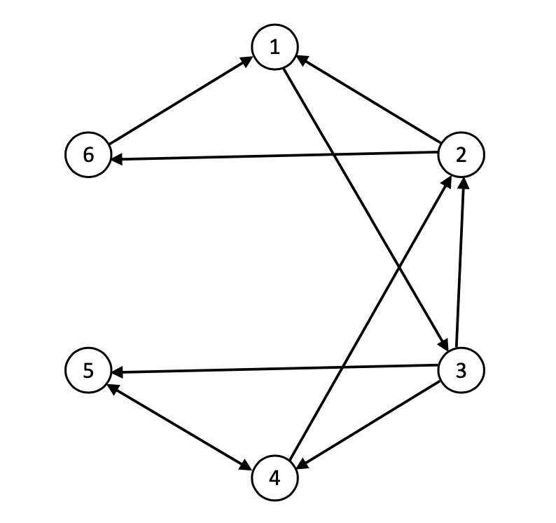
Figure 2: Illustration of the network topology of six oscillators (agents) where the weight associated with each edge (arrowed line) is positive.

In particular, the following function

$$K(\hat{x})=K_{o}\frac{\hat{x}^{\mbox{\tiny\sf T}}}{\|\hat{x}\|^{2}}\left[\begin{array}[]{cc}0&-1\\ 1&0\end{array}\right],\;K_{o}=\left[\begin{array}[]{c}1.80\\ 1.76\end{array}\right]$$

with

$$K^{\prime}(x,\hat{x},\hat{\sigma})= K_{o}\left(\frac{I_{q}-2f(\hat{x})f^{\mbox{\tiny\sf T}}(\hat{x})}{\|\hat{x}\|^{2}}\times\right.$$

$$\left.\left[\begin{array}[]{cc}0&1\\ -1&0\end{array}\right]\left(f(x)\hat{\omega}+\kappa(x,\hat{x})\right)\right)^{\mbox{\tiny\sf T}}$$

is used to construct the functions $\mu$ and $\kappa$ of the frequency observers. The parameter $\beta=10$ is used for the simulation. It is noted that a higher value of $\beta$ gives faster convergence of the frequency observers. For $a_{ij}=1,\;\forall\left(i,j\right)\in\mathcal{E}$, the control gain matrix $M=0.01\left[\begin{array}[]{cc}1&0.5\end{array}\right]$ representing weak coupling among the oscillators is used in the controller. Using the observer/controller proposed in the paper, the synchronization performance of the oscillators is discussed below. In the figures, we only demonstrate the trajectories of three oscillators, denoted as OSC 1, OSC 3, and OSC 5, corresponding to the nodes 1, 3, and 5 in Fig. 2, respectively. The other three oscillators have similar profiles and thus omitted.

The profile of the frequency modulated signals $x_{i}(t)$ (only the first component $x_{i1}(t)$ for concise presentation) is shown in Fig. 5. Frequency synchronization can be observed in this figure as expected, while synchronization of the signals in oscillation phase and amplitudes is not needed. Frequency synchronization can also be exhibited in Fig. 5 in an explicit illustration. It is noted that frequencies $\omega_{i}(t)$ in this figure are not directly measured or transmitted via the network. The effectiveness of the proposed frequency observer is verified in Fig. 5. According to the topology, the frequency of OSC 1 is observed by agent 3, that of OSC 3 is observed by agents 2, 4, 5, separately, and that of OSC 5 by agent 4. The convergence of the observed frequencies (in dashed curves) to the real values (solid curves) can be achieved by all the observers .

Next, we examine the robustness of synchronization of frequency modulated oscillators with respect to noise in the transmitted signals via the network. The result is shown in Fig. 6 using the synchronization error $\omega_{1}(t)-\omega_{3}(t)$ as an example. The top graph shows a perfect synchronization behavior without any noticeable error in the scale of $\pm 0.01$. The relative and absolute error tolerances in MATLAB simulation are $10^{-4}$ and $10^{-8}$, respectively. The middle graph shows the result for the unmodulated controller (4) with transmission noise, i.e,

$$\chi_{i}=-M\sum_{j\in{\cal N}_{i}}a_{ij}(\sigma_{i}-\sigma_{j}-{\rm n}^{i}_{j}),\;i\in\mathcal{V}$$

where the level of noise ${\rm n}^{i}_{j}$ on $\sigma_{j}$ transmitted from $j$ to $i$ is $\pm 1\%$ of the magnitude of the transmitted signals. In this case, the synchronization error induced by the noise can ben obviously observed. Finally, we apply the same level of noise on the frequency modulated controller (7), i.e.,

$$\dot{\hat{\sigma}}_{j}^{i} =S\hat{\sigma}_{j}^{i}+\mu(x_{j}+{\rm n}^{i}_{j},\hat{x}_{j}^{i},\hat{\sigma}_{j}^{i})$$

$$\hat{\omega}_{j}^{i} =E\hat{\sigma}_{j}^{i}+\omega_{c}$$

$$\dot{\hat{x}}_{j}^{i} =f(\hat{x}^{i}_{j})\hat{\omega}_{j}^{i}+f_{o}(x_{j}+{\rm n}^{i}_{j})+\kappa(x_{j}+{\rm n}^{i}_{j},\hat{x}_{j}^{i}),\;j\in{\cal N}_{i}.$$

The result in the bottom graph exhibits that the synchronization error using frequency modulation is significantly less than that in the unmodulated case. The error is noticeable with more details when it is amplified to the scale of $10^{-4}$. The comparison in Fig. 6 verifies the robustness of frequency modulated MASs in mitigating the influence of network noise.

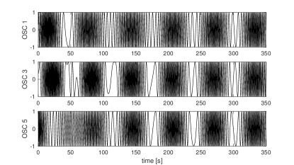
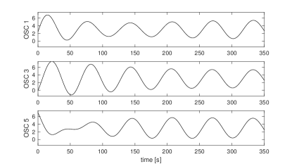
Figure 3: Profile of the frequency modulated signals $x_{i1}(t)$, the first element of the state vector $x_{i}(t)$, for $i=1,3,5$.

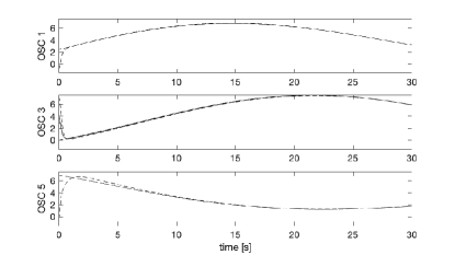
Figure 4: Profile of the frequencies $\omega_{i}(t)$ for $i=1,3,5$.

Figure 5: Profile of the observed frequencies $\hat{\omega}_{j}^{i}(t)$, $j\in{\cal N}_{i}$ (dashed curves) vs the real frequencies $\omega_{j}(t)$ (solid curves), for $j=1,3,5$.

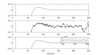
Figure 6: Profile of the synchronization error $\omega_{1}(t)-\omega_{3}(t)$ in three cases. Top graph: noise free; middle graph: unmodulated synchronization with noise; and bottom graph: frequency modulated synchronization with noise.

Next, we consider another example of a network of Hindmarsh-Rose oscillators, which are a class of low-dimensional Hodgkin-Huxley model of neuronal activity. They can characterize the spiking-bursting behavior of the membrane potential observed in experiments. The dynamics are of the form (1) with

$$S=\left[\begin{array}[]{cc}0&0.005\pi\\ -0.005\pi&0\end{array}\right],\;B=\left[\begin{array}[]{c}1\\ 1\end{array}\right],\;E=\left[\begin{array}[]{cc}0.4&0\end{array}\right]$$

and

$$x_{i}=\left[\begin{array}[]{c}v_{i}\\ w_{i}\\ z_{i}\end{array}\right],\;f(x_{i})=\left[\begin{array}[]{c}2\\ -5v_{i}^{2}-w_{i}+1\\ 0\end{array}\right],$$

$$f_{o}(x_{i})=\left[\begin{array}[]{c}3v_{i}^{2}-v_{i}^{3}+w_{i}-z_{i}\\ 0\\ 0.005(4(v_{i}+1.5)-z_{i})\end{array}\right],\;\omega_{c}=0.9.$$

The variable $v_{i}(t)$ represents the membrane potential of a neuron, $w_{i}(t)$ is the spiking variable that represents the transport rate of sodium and potassium ions through fast ion channels, and $z_{i}(t)$ is the adaptation current that increases at every spike and leads to a decrease in the firing rate. The signal $\omega_{i}(t)$ is encoded as the firing rate of the membrane potential. The network topology is the same one in Fig. 2. The non-sinusoidal signals $x_{i}(t)$ of this class of oscillators consist of bursts and spikes of varying firing rates. The synchronization target is not the instantaneous signals but their firing rates.

The results discussed in the first example can be observed in this example as well. As a comparison, the membrane potentials of the individual oscillators without synchronization control, i.e., $\chi_{i}=0$, are plotted in Fig. 7. With the synchronization controller proposed in this paper, frequency synchronization of membrane potentials is plotted in Fig. 10 and synchronization of firing rates of spikes in Fig. 10. Once synchronized, the firing rates of spikes are generally less than those of individual oscillators because the variations of the firing rates are averaged. It is also noted that the signals in terms of the instantaneous values are not necessarily synchronized. The convergence of the observed firing rates to the real values is shown in Fig. 10. The results well demonstrate the similar phenomenon observed in real neural circuits.

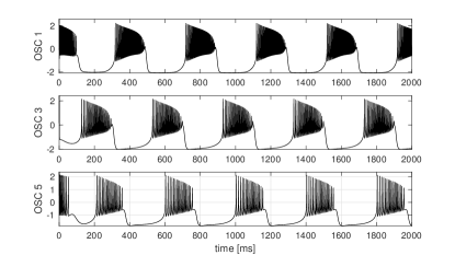
Figure 7: Profile of the membrane potentials $v_{i}(t)$ of individual Hindmarsh-Rose oscillators without synchronization for $i=1,3,5$.

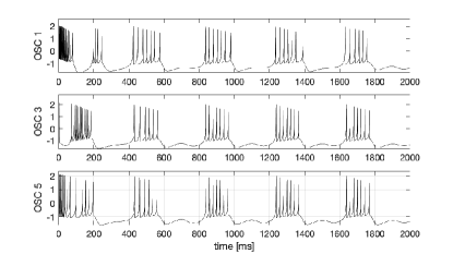
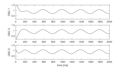
Figure 8: Profile of the membrane potentials $v_{i}(t)$ of Hindmarsh-Rose oscillators for $i=1,3,5$.

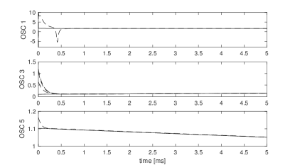
Figure 9: Profile of the firing rates $\omega_{i}(t)$ of Hindmarsh-Rose oscillators for $i=1,3,5$.

Figure 10: Profile of the observed firing rates $\hat{\omega}_{j}^{i}(t)$, $j\in{\cal N}_{i}$ (dashed curves) vs the real firing rates $\omega_{j}(t)$ (solid curves) of Hindmarsh-Rose oscillators for $j=1,3,5$.

VII Conclusions

In this paper, we have established a framework for synchronization of frequency modulated multi-agent systems for the first time. The framework includes a frequency observer subject to an external input and a distributed synchronization controller based on the observer using the small gain argument. We have verified the effectiveness of the design using rigorous theoretical proofs and extensive numerical simulation. It is interesting to further extend the framework to study more complicated models, especially from real biological neural networks. The research for unmodulated multi-agent systems has experienced rapid development in the recent decade, which can be further developed for frequency modulated multi-agent systems using the framework in this paper. The robust synchronization mechanism using frequency modulated signals has the potentials in revealing the similar phenomenon in real systems and gaining deep understanding of how neuronal circuits generate extremely robust and adaptive oscillatory behaviors in animal locomotion. It is expected that the research along this direction is also beneficial for building artificial frequency modulated multi-agent systems with more engineering applications.

References

- [1] W. Gerstner, A. K. Kreiter, H. Markram, and A. V. Herz, “Neural codes: firing rates and beyond,” Proceedings of the National Academy of Sciences, vol. 94, no. 24, pp. 12 740–12 741, 1997.
- [2] J. M. Newcomb, A. Sakurai, J. L. Lillvis, C. A. Gunaratne, and P. S. Katz, “Homology and homoplasy of swimming behaviors and neural circuits in the nudipleura (mollusca, gastropoda, opisthobranchia),” Proceedings of the National Academy of Sciences, vol. 109, no. Supplement 1, pp. 10 669–10 676, 2012.
- [3] J. Saeedi and K. Faez, “Synthetic aperture radar imaging using nonlinear frequency modulation signal,” IEEE Transactions on Aerospace and Electronic Systems, vol. 52, no. 1, pp. 99–110, 2016.
- [4] H.-J. Choi and J.-H. Jung, “Enhanced power line communication strategy for DC microgrids using switching frequency modulation of power converters,” IEEE Transactions on Power Electronics, vol. 32, no. 6, pp. 4140–4144, 2017.
- [5] Z. Wang, Y. Wang, and L. Xu, “Parameter estimation of hybrid linear frequency modulation-sinusoidal frequency modulation signal,” IEEE Signal Processing Letters, vol. 24, no. 8, pp. 1238–1241, 2017.
- [6] M. A. Lewis, F. Tenore, and R. Etienne-Cummings, “CPG design using inhibitory networks,” in Proceedings of the 2005 IEEE International Conference on Robotics and Automation. IEEE, 2005, pp. 3682–3687.
- [7] A. J. Ijspeert, A. Crespi, D. Ryczko, and J.-M. Cabelguen, “From swimming to walking with a salamander robot driven by a spinal cord model,” Science, vol. 315, no. 5817, pp. 1416–1420, 2007.
- [8] A. Spaeth, M. Tebyani, D. Haussler, and M. Teodorescu, “Spiking neural state machine for gait frequency entrainment in a flexible modular robot,” PloS One, vol. 15, no. 10, p. e0240267, 2020.
- [9] E. O. Olivares, E. J. Izquierdo, and R. D. Beer, “Potential role of a ventral nerve cord central pattern generator in forward and backward locomotion in caenorhabditis elegans,” Network Neuroscience, vol. 2, no. 3, pp. 323–343, 2018.
- [10] L. Hachoumi and K. T. Sillar, “Developmental stage-dependent switching in the neuromodulation of vertebrate locomotor central pattern generator networks,” Developmental Neurobiology, vol. 80, no. 1-2, pp. 42–57, 2020.
- [11] W. Friesen and C. Hocker, “Functional analyses of the leech swim oscillator,” J. Neurophysiol., vol. 86, pp. 824–835, 2001.
- [12] Z. Chen, M. Zheng, W. O. Friesen, and T. Iwasaki, “Multivariable harmonic balance analysis of neuronal oscillator for leech swimming,” Journal of Computational Neuroscience, vol. 25, pp. 583–606, 2008.
- [13] T. Iwasaki, J. Chen, and W. O. Friesen, “Biological clockwork underlying adaptive rhythmic movements,” Proceedings of the National Academy of Sciences, vol. 111, no. 3, pp. 978–983, 2014.
- [14] A. Jadbabaie, J. Lin, and A. S. Morse, “Coordination of groups of mobile agents using nearest neighbor rules,” IEEE Transactions on Automatic Control, vol. 48, no. 6, pp. 988–1001, 2003.
- [15] R. Olfati-Saber and R. Murray, “Consensus problems in networks of agents with switching topology and time-delays,” IEEE Transactions on Automatic Control, vol. 49, no. 9, pp. 1520–1533, 2004.
- [16] W. Ren and R. W. Beard, “Consensus seeking in multiagents systems under dynamically changing interaction topologies,” IEEE Transactions on Automatic Control, vol. 50, no. 5, pp. 655–661, 2005.
- [17] L. Scardovi and R. Sepulchre, “Synchronization in networks of identical linear systems,” Automatica, vol. 45, no. 11, pp. 2557–2562, 2009.
- [18] S. E. Tuna, “LQR-based coupling gain for synchronization of linear systems,” arXiv preprint arXiv:0801.3390, 2008.
- [19] J. Seo, H. Shim, and J. Back, “Consensus of high-order linear systems using dynamic output feedback compensator: Low gain approach,” Automatica, vol. 45, no. 11, pp. 2659–2664, 2009.
- [20] S. E. Tuna, “Synchronizing linear systems via partial-state coupling,” Automatica, vol. 44, no. 8, pp. 2179–2184, 2008.
- [21] K. You and L. Xie, “Network topology and communication data rate for consensusability of discrete-time multi-agent systems,” IEEE Transactions on Automatic Control, vol. 56, no. 10, pp. 2262–2275, 2011.
- [22] K. Hengster-Movric, K. You, F. L. Lewis, and L. Xie, “Synchronization of discrete-time multi-agent systems on graphs using riccati design,” Automatica, vol. 49, no. 2, pp. 414–423, 2013.
- [23] A. A. Stoorvogel, A. Saberi, M. Zhang, and Z. Liu, “Solvability conditions and design for synchronization of discrete-time multiagent systems,” International Journal of Robust and Nonlinear Control, vol. 28, no. 4, pp. 1381–1401, 2018.
- [24] S. Knorn, Z. Chen, and R. H. Middleton, “Overview: Collective control of multiagent systems,” IEEE Transactions on Control of Network Systems, vol. 3, no. 4, pp. 334–347, Dec 2016.
- [25] H. Modares, B. Kiumarsi, F. L. Lewis, F. Ferrese, and A. Davoudi, “Resilient and robust synchronization of multiagent systems under attacks on sensors and actuators,” IEEE Transactions on Cybernetics, vol. 50, no. 3, pp. 1240–1250, 2019.
- [26] G. Jing and L. Wang, “Multiagent flocking with angle-based formation shape control,” IEEE Transactions on Automatic Control, vol. 65, no. 2, pp. 817–823, 2019.
- [27] P. Wieland, R. Sepulchre, and F. Allgöwer, “An internal model principle is necessary and sufficient for linear output synchronization,” Automatica, vol. 47, no. 5, pp. 1068–1074, 2011.
- [28] H. Kim, H. Shim, and J. H. Seo, “Output consensus of heterogeneous uncertain linear multi-agent systems,” IEEE Transactions on Automatic Control, vol. 56, no. 1, pp. 200–206, 2011.
- [29] T. Yang, A. Saberi, A. A. Stoorvogel, and H. F. Grip, “Output synchronization for heterogeneous networks of introspective right-invertible agents,” International Journal of Robust and Nonlinear Control, vol. 24, no. 13, pp. 1821–1844, 2014.
- [30] L. Zhu and Z. Chen, “Robust homogenization and consensus of nonlinear multi-agent systems,” Systems and Control Letters, vol. 65, pp. 50–55, 2014.
- [31] J. Lunze, “Synchronization of heterogeneous agents,” IEEE Transactions on Automatic Control, vol. 57, no. 11, pp. 2885–2890, 2012.
- [32] H. Grip, A. Saberi, and A. Stoorvogel, “On the existence of virtual exosystems for synchronized linear networks,” Automatica, vol. 49, no. 10, pp. 3145–3148, 2013.
- [33] W. Yu, G. Chen, and M. Cao, “Consensus in directed networks of agents with nonlinear dynamics,” IEEE Transactions on Automatic Control, vol. 56, no. 6, pp. 1436–1441, 2011.
- [34] H. Su, G. Chen, X. Wang, and Z. Lin, “Adaptive second-order consensus of networked mobile agents with nonlinear dynamics,” Automatica, vol. 47, no. 2, pp. 368–375, 2011.
- [35] L. Pecora and T. Carroll, “Synchronization in chaotic systems,” Physical Review Letters, vol. 64, no. 8, p. 821, 1990.
- [36] N. Chopra and M. Spong, “On exponential synchronization of Kuramoto oscillators,” IEEE Transactions on Automatic Control, vol. 54, no. 2, pp. 353–357, 2009.
- [37] H. Su, X. Wang, and Z. Lin, “Synchronization of coupled harmonic oscillators in a dynamic proximity network,” Automatica, vol. 45, no. 10, pp. 2286–2291, 2009.
- [38] A. Isidori, L. Marconi, and G. Casadei, “Robust output synchronization of a network of heterogeneous nonlinear agents via nonlinear regulation theory,” IEEE Transactions on Automatic Control, vol. 59, no. 10, pp. 2680–2691, 2014.
- [39] X. Chen and Z. Chen, “Robust perturbed output regulation and synchronization of nonlinear heterogeneous multiagents,” IEEE Transactions on Cybernetics, vol. 46, no. 12, pp. 3111–3122, 2015.
- [40] L. Zhu, Z. Chen, and R. Middleton, “A general framework for robust output synchronization of heterogeneous nonlinear networked systems,” IEEE Transactions on Automatic Control, vol. 61, no. 8, pp. 2092–2107, 2016.
- [41] Y. Su and J. Huang, “Cooperative global robust output regulation for nonlinear uncertain multi-agent systems in lower triangular form,” IEEE Transactions on Automatic Control, vol. 60, no. 9, pp. 2378–2389, 2015.
- [42] H. Cai, F. L. Lewis, G. Hu, and J. Huang, “The adaptive distributed observer approach to the cooperative output regulation of linear multi-agent systems,” Automatica, vol. 75, pp. 299–305, 2017.
- [43] J. Huang, “The cooperative output regulation problem of discrete-time linear multi-agent systems by the adaptive distributed observer,” IEEE Transactions on Automatic Control, vol. 62, no. 4, pp. 1979–1984, 2017.
- [44] Y. Yan and Z. Chen, “Cooperative output regulation of linear discrete-time time-delay multi-agent systems by adaptive distributed observers,” Neurocomputing, vol. 331, pp. 33–39, 2019.
- [45] E. Panteley, A Stability-Theory Perspective to Synchronization of Heterogeneous Networks (Drsc Dissertation). University Paris Sud, Orsay, France, 2015.
- [46] E. Panteley and A. Loría, “Synchronization and dynamic consensus of heterogeneous networked systems,” IEEE Transactions on Automatic Control, vol. 62, no. 8, pp. 3758–3773, 2017.
- [47] M. Maghenem, E. Panteley, and A. Loria, “Singular-perturbations-based analysis of synchronization in heterogeneous networks: A case-study,” in 2016 IEEE 55th Conference on Decision and Control (CDC), 2016, pp. 2581–2586.
- [48] E. Panteley, A. Loria, and A. El-Ati, “Practical dynamic consensus of Stuart-Landau oscillators over heterogeneous networks,” International Journal of Control, vol. 93, no. 2, pp. 261–273, 2020.
- [49] Y. Yan, Z. Chen, and R. Middleton, “Autonomous synchronization of heterogeneous multi-agent systems,” IEEE Transactions on Control of Network Systems, 2020, DOI: 10.1109/TCNS.2020.3042593.
- [50] Z. Hu, Z. Chen, and H. T. Zhang, “Necessary and sufficient conditions for asymptotic decoupling of stable modes in LTV systems,” IEEE Transactions on Automatic Control, 2020, DOI: 10.1109/TAC.2020.3030854.
- [51] Z. Chen and J. Huang, Stabilization and Regulation of Nonlinear Systems. Springer, 2005.
- [52] X.-H. Xia and W.-B. Gao, “Nonlinear observer design by observer error linearization,” SIAM Journal on Control and Optimization, vol. 27, no. 1, pp. 199–216, 1989.
- [53] M. Zeitz, “The extended Luenberger observer for nonlinear systems,” Systems and Control Letters, vol. 9, no. 2, pp. 149–156, 1987.
- [54] H. K. Khalil and L. Praly, “High-gain observers in nonlinear feedback control,” International Journal of Robust and Nonlinear Control, vol. 24, no. 6, pp. 993–1015, 2014.
- [55] D. Astolfi and L. Marconi, “A high-gain nonlinear observer with limited gain power,” IEEE Transactions on Automatic Control, vol. 60, no. 11, pp. 3059–3064, 2015.