MatSat: a matrix-based differentiable SAT solver

Abstract

We propose a new approach to SAT solving which solves SAT problems in vector spaces as cost minimization of a differentiable cost function ${\rm J}^{sat}$. In our approach, a solution, satisfying assignment, of a SAT problem in $n$ variables is represented by a binary vector ${\mathbf{u}}\in\{0,1\}^{n}$ such that ${\rm J}^{sat}({\mathbf{u}})=0$. We search for such ${\mathbf{u}}$ in a vector space $\mathbb{R}^{n}$ by cost minimization, i.e., starting from an initial ${\mathbf{u}}_{0}$, we minimize ${\rm J}^{sat}$ to zero while iteratively updating ${\mathbf{u}}$ by Newton’s method. We implemented our approach as an incomplete matrix-based differentiable SAT solver MatSat. Although existing main-stream SAT solvers decide each bit of a solution assignment one by one, be they of conflict driven clause learning (CDCL) type or of stochastic local search (SLS) type, MatSat fundamentally differs from them in that it updates all variables at once and continuously approaches a solution in a vector space. We conducted experiments to measure the scalability of MatSat with random 3-SAT problems. In these experiments, for example, we showed that MatSat implemented on GPU can solve the problem with $n=3\times 10^{5}$ variables, demonstrating the feasibility of hardware acceleration by GPU for matrix-based solvers like MatSat. We also compared MatSat with nine state-of-the-art CDCL and SLS SAT solvers in terms of execution time by conducting experiments with several random and non-random data sets. In the case of easy random SAT, the performance of MatSat comes between the SLS solvers and the CDCL solvers whereas it is ranked 1st on the difficult one. On the other hand, MatSat showed poor performance on non-random SAT problems. To improve its poor performance, we introduced weighted variables and clauses and confirmed the effectiveness of the weighted version of MatSat on non-random SAT.

0.1 Introduction

The Boolean satisfiability problem (SAT) lies at the core of many fields including AI and extensive efforts have been made to build powerful SAT solvers. In this paper, we propose a new approach to SAT solving which solves SAT problems as cost minimization of a differentiable cost function ${\rm J}^{sat}$ in vector spaces that contains a piecewise linear function $\mbox{min}_{1}(x)=\mbox{min}(x,1)$ as a continuous surrogate for disjunction.

In our approach, a solution of a SAT problem in $n$ variables is represented by a 0-1 vector ${\mathbf{u}}\in\{0,1\}^{n}$ such that ${\rm J}^{sat}({\mathbf{u}})=0$, i.e., ${\mathbf{u}}$ is a root of ${\rm J}^{sat}$. We search for such ${\mathbf{u}}$ in a vector space $\mathbb{R}^{n}$ by cost minimization, i.e., starting from a random ${\mathbf{u}}_{0}$, we minimize ${\rm J}^{sat}$ to zero while iteratively updating ${\mathbf{u}}$ using Newton’s method. We implemented our approach as a matrix-based differentiable SAT solver MatSat. While existing main-stream SAT solvers search for a solution by determining each bit of a candidate assignment one by one, be they of conflict driven clause learning (CDCL) type or of stochastic local search (SLS) type, MatSat fundamentally differs from them in that it updates all variables at once and continuously approaches a solution in a high dimensional vector space with help of gradient information.

In a broader perspective, MatSat is considered as an embodiment of recently emerging differentiable approaches which solve logical problems by converting them to differentiable forms in a continuous space. We pick up some of them here as the background of our work. In the field of logic programming, Sato finds that Datalog programs can be computed orders of magnitude faster than the traditional symbolic evaluation by way of matrix equations [23]. Also it is shown that inventing new predicates can be carried out on a large scale in a vector space by minimizing a loss function made up of matrices representing them [24]. Sakama et al. developed a matrix-based approach to partial evaluation of logic programs [22].

Aside from these logic-based approaches, there are differentiable approaches closer to neural networks. Evans and Grefenstette showed how to incorporate differentiable components into an inductive logic programming framework by learning a weight matrix associated with candidate clauses for a target program to be synthesized [8]. Manhaeve et al.  presented a neural extension of probabilistic modeling language ProbLog allowing “neural predicates” whose probabilities are computed by neural networks [18]. Cingillioglu and Russo described a way of handling logical entailment in logic programs by their Iterative Memory Attention model that manipulates a vectorized normal logic program and a vectorized query atom [6].

The approaches described above deal with logic in one way or another but are not directly aimed at SAT solving. There are however researchers aiming at differentiable SAT solvers. For example, Nickles incorporated a differentiable evaluation function into a SAT solver to choose a decision literal for sampling of answer sets in probabilistic answer set programming [19]. Wang et. al built a MAXSAT solver based on the combination of semidefinite programming relaxation and branch-and-bound strategy [29]. Selsam et al.  proposed a neural net classifier NeuroSAT for SAT problems that learn embeddings of a SAT problem through three perceptrons and two LSTMs so that the system predicts one bit, i.e., the satisfiability of the problem [27].

Compared to these differentiable SAT solvers, the architecture of MatSat is quite simple. When viewed as a neural network, it is just a one-layer neural network applying a piecewise linear activating function and sum-product operation to a matrix describing a SAT problem. From the viewpoint of existing SAT solvers, MatSat is an incomplete solver unable to solve UNSAT problems. Nonetheless when applied to SAT problems, it sometimes outperforms state-of-the-art SAT solvers as far as experimental results in Section 0.5 are concerned. It is also scalable, solving random 3-SAT problems with up to $3\times 10^{5}$ variables when implemented on GPU.

Our contributions thus include a reformulation of SAT solving as cost minimization in vector spaces with a logic-based cost function, a proposal of matricized differentiable SAT solver MatSat suited for multicore and GPU architecture, and experimental demonstration of the strength of MatSat together with its weakness.

0.2 Preliminaries

In this paper, bold italic capital letters such as $\bm{A}$ stand for a real matrix whereas bold italic lower case letters such as $\bm{a}$ stand for a real vector. $\|\bm{a}\|_{1}=\sum_{i}|\bm{a}(i)|$ denotes the 1-norm of a vector $\bm{a}$ and $\|\bm{a}\|_{2}=\sqrt{\sum_{i}\bm{a}(i)^{2}}$ is the 2-norm of $\bm{a}$. For two $n$ dimensional vectors $\bm{a}$ and $\bm{b}$, we use $(\bm{a}\bullet\bm{b})$ to denote their inner product (dot product) and $\bm{a}\odot\bm{b}$ to denote their Hadamard product, i.e., $(\bm{a}\odot\bm{b})(i)=\bm{a}(i)\bm{b}(i)$ for $i(1\leq i\leq n)$. The dimension $n$ of a vector $\bm{a}$ is sometimes called the length of $\bm{a}$. For a scalar $\theta$, $\bm{a}_{<\theta}$ stands for a binary vector such that $\bm{a}_{<\theta}(i)=1$ if $\bm{a}(i)<\theta$ and $\bm{a}_{<\theta}(i)=0$ otherwise. ${\mathbf{1}}_{m}$ designates an all-one column vector of length $m$. $\mbox{min}_{1}(x)=\mbox{min}(x,1)$ designates the lesser of 1 and $x$. $\mbox{min}_{1}(\bm{a})$ means the component-wise application of $\mbox{min}_{1}(x)$ to a vector $\bm{a}$.

0.3 Matricized SAT

We encode a SAT instance in CNF form with $m$ clauses in $n$ variables into an $m\times 2n$ binary matrix. For example, we encode a SAT instance $S_{0}=(a\vee b\vee\bar{c})\wedge(\bar{a}\vee\bar{b})$ into ${\mathbf{Q}}_{0}\in\mathbb{R}^{2\times 3}$ below.

$${\mathbf{Q}}_{0}=\begin{array}[]{c}\begin{array}[]{cccccc}a&b&c&\bar{a}&\bar{b}&\bar{c}\\ \end{array}\\ \left[\begin{array}[]{cccccc}1&1&0&0&0&1\\ 0&0&0&1&1&0\\ \end{array}\right]\end{array}$$

The idea behind ${\mathbf{Q}}_{0}$ is that when a SAT instance $S=C_{1}\wedge\cdots\wedge C_{m}$ of $m$ clauses in $n$ variables $\{a_{1},\ldots,a_{n}\}$ is given, we introduce $2n$ literals $\{a_{1},\ldots,a_{n},\neg a_{1},\ldots,\neg a_{n}\}$ in this order together with a binary matrix ${\mathbf{Q}}\in\{0,1\}^{m\times 2n}$ and use them as a column index for ${\mathbf{Q}}$. ${\mathbf{Q}}$ represents $S$ in such a way that $\bm{Q}(i,:)$, the $i$-th row in $\bm{Q}$, encodes the $i$-th clause $C_{i}$ ($1\leq i\leq m$). More concretely, when the $i$-th clause $C_{i}$ ($1\leq i\leq m$) contains a positive literal $a_{j}$($1\leq j\leq n$) (resp. negative literal $\neg a_{j}$), we put ${\mathbf{Q}}(i,j)=1$ (resp. ${\mathbf{Q}}(i,j+n)=1$). Otherwise ${\mathbf{Q}}(i,j)={\mathbf{Q}}(i,j+n)=0$. We call ${\mathbf{Q}}$ an instance matrix for $S$. A truth value assignment (interpretation) for $\{a_{1},\ldots,a_{n}\}$ is identified with an assignment vector, i.e., a binary column vector ${\mathbf{u}}\in\{0,1\}^{n}$ of length $n$ such that ${\mathbf{u}}(j)=1$ (resp. $0$) holds if-and-only-if the variable $a_{j}$ is true (resp. false) in the assignment ($1\leq j\leq n$). Henceforth we interchangeably use 1 for true and 0 for false.

Now introduce the dualized assignment vector ${\mathbf{u}}^{d}=[{\mathbf{u}};{\mathbf{1}}_{n}-{\mathbf{u}}]$ of ${\mathbf{u}}$. It is a vertical concatenation of two column vectors ${\mathbf{u}}$ and its complement ${\mathbf{1}}_{n}-{\mathbf{u}}$. Put $\delta_{i}=\bm{Q}(i,:){\mathbf{u}}^{d}$. It is immediate to see that $\delta_{i}$ gives the number of literals true in ${\mathbf{u}}$ contained in $C_{i}$. So if $\delta_{i}\geq 1$, or equivalently, if $\mbox{min}_{1}(\delta_{i})=1$, we know that $C_{i}$ is true in ${\mathbf{u}}$. Otherwise $\mbox{min}_{1}(\delta_{i})=0$ and $C_{i}$ is false in ${\mathbf{u}}$. Thus a clause $C_{i}$ is evaluated by ${\mathbf{u}}$ to $\mbox{min}_{1}(\delta_{i})=\mbox{min}_{1}(\bm{Q}(i,:){\mathbf{u}}^{d})\in\{0,1\}$ and if all $\mbox{min}_{1}(\delta_{i})$’s are 1, in other words, if $\mbox{min}_{1}(\bm{Q}{\mathbf{u}}^{d})={\mathbf{1}}_{m}$ holds, $S$ is satisfiable and ${\mathbf{u}}$ is a solution, i.e., satisfying assignment. We summarize discussion so far as Proposition 1.

Proposition 1.

Let $\bm{Q}\in\{0,1\}^{m\times 2n}$ be an instance matrix for a SAT instance $S=C_{1}\wedge\cdots\wedge C_{m}$ with $m$ clauses in $n$ variables and ${\mathbf{u}}$ an assignment for the variables in $S$. $S$ is satisfiable if-and-only-if $\mbox{min}_{1}(\bm{Q}{\mathbf{u}}^{d})={\mathbf{1}}_{m}$.

Proof.

We prove the only-if part. Suppose $S$ is satisfiable and has a satisfying assignment ${\mathbf{u}}$. For every $i$ ($1\leq i\leq m$), $C_{i}$ has at least one literal true in ${\mathbf{u}}$. So $\delta_{i}=\bm{Q}(i,:){\mathbf{u}}^{d}\geq 1$ and hence $\mbox{min}_{1}(\bm{Q}(i,:){\mathbf{u}}^{d})=1$ holds for every $i$, which means $\mbox{min}_{1}(\bm{Q}{\mathbf{u}}^{d})$ is an all-one vector ${\mathbf{1}}_{m}$. ∎

Consider for example an assignment ${\mathbf{u}}_{0}=[1\;0\;0]^{T}$ for the variables $\{a,b,c\}$ in $S_{0}$. Then we have ${\mathbf{u}}_{0}^{d}=[1\;0\;0\;0\;1\;1]^{T}$ and $\delta_{1}=\bm{Q}_{0}(1,:){\mathbf{u}}_{0}^{d}=2$. Accordingly $\mbox{min}_{1}(\delta_{1})=1$ and the first clause $a\vee b\vee\bar{c}$ in $S_{0}$ is true in ${\mathbf{u}}_{0}$. Likewise $\mbox{min}_{1}(\delta_{2})=\mbox{min}_{1}(\bm{Q}_{0}(2,:){\mathbf{u}}_{0}^{d})=1$ and the second clause $\neg a\vee\neg b$ is true in ${\mathbf{u}}_{0}$ as well. So all clauses are true in ${\mathbf{u}}_{0}$, i.e., $\mbox{min}_{1}(\bm{Q}_{0}{\mathbf{u}}_{0}^{d})=[1\;1]^{T}={\mathbf{1}}_{2}$ in notation and ${\mathbf{u}}_{0}$ is a solution for the SAT instance $S_{0}$.

0.4 SAT solving by cost minimization

According to Proposition 1, SAT solving is equivalent to finding an assignment vector ${\mathbf{u}}\in\{0,1\}^{n}$ making $\mbox{min}_{1}(\bm{Q}{\mathbf{u}}^{d})={\mathbf{1}}_{m}$ true where ${\mathbf{Q}}\in\{0,1\}^{m\times 2n}$ is an instance matrix for $m$ clauses in $n$ variables. We solve this problem by cost minimization applied to a relaxed equation $\mbox{min}_{1}(\bm{Q}{\tilde{\mathbf{u}}}^{d})={\mathbf{1}}_{m}$ for $\tilde{\mathbf{u}}\in\mathbb{R}^{n}$ where $\tilde{\mathbf{u}}^{d}=[\tilde{\mathbf{u}};{\mathbf{1}}_{n}-\tilde{\mathbf{u}}]$. We first introduce a cost function ${\rm J}^{sat}:\tilde{\mathbf{u}}\in\mathbb{R}^{n}\mapsto\mathbb{R}$ below where $\ell>0$.

$${\rm J}^{sat} = ({\mathbf{1}}_{m}\bullet({\mathbf{1}}_{m}-\mbox{min}_{1}({\mathbf{Q}}\tilde{\mathbf{u}}^{d})))+(\ell/2)\cdot\|\tilde{\mathbf{u}}\odot({\mathbf{1}}_{n}-\tilde{\mathbf{u}})\|_{2}^{2}$$ (1)

Proposition 2.

Let $\bm{Q}\in\{0,1\}^{m\times 2n}$ be an instance matrix for a SAT instance $S$. ${\rm J}^{sat}=0$ if-and-only-if $\tilde{\mathbf{u}}$ is a binary vector $\in\{0,1\}^{n}$ and $\tilde{\mathbf{u}}$ represents a satisfying assignment for $S$.

Proof.

Let $\tilde{\mathbf{u}}$ be an assignment vector satisfying $S$. Then by Proposition 1, we have ${\mathbf{1}}_{m}=\mbox{min}_{1}({\mathbf{Q}}\tilde{\mathbf{u}}^{d})$. So the first term in ${\rm J}^{sat}$ is zero. Since $\tilde{\mathbf{u}}\in\{0,1\}^{n}$, the second term in ${\rm J}^{sat}$ is zero as well. Hence ${\rm J}^{sat}=0$. Now suppose ${\rm J}^{sat}=0$. Since every term in ${\rm J}^{sat}$ is non-negative, we have $({\mathbf{1}}_{m}\bullet({\mathbf{1}}_{m}-\mbox{min}_{1}({\mathbf{Q}}\tilde{\mathbf{u}}^{d})))=0$ and $\|\tilde{\mathbf{u}}\odot({\mathbf{1}}_{n}-\tilde{\mathbf{u}})\|_{2}^{2}=0$. The latter implies $\tilde{\mathbf{u}}$ is a binary vector whereas the former implies that ${\mathbf{1}}_{m}-\mbox{min}_{1}({\mathbf{Q}}\tilde{\mathbf{u}}^{d})={\mathbf{0}}$, i.e., $\mbox{min}_{1}({\mathbf{Q}}\tilde{\mathbf{u}}^{d})={\mathbf{1}}_{m}$ holds. Therefore every clause in $S$ is true in $\tilde{\mathbf{u}}$. ∎

Proposition 2 tells us that a SAT solution is a root of ${\rm J}^{sat}$. So we compute it by Newton’s method. We need the Jacobian ${\mathbf{J}}_{acb}^{sat}$ of ${\rm J}^{sat}$. Split ${\mathbf{Q}}$ into ${\mathbf{Q}}=[{\mathbf{Q}}_{1}\,{\mathbf{Q}}_{2}]$ where ${\mathbf{Q}}_{1}\in\{0,1\}^{m\times n}$ is a binary matrix holding occurrence information about positive literals in each clause while ${\mathbf{Q}}_{2}\in\{0,1\}^{m\times n}$ is the one about negative literals. ${\mathbf{J}}_{acb}^{sat}$ is derived as follows.

Put ${\mathbf{c}}={\mathbf{Q}}\tilde{\mathbf{u}}^{d}={\mathbf{Q}}_{2}{\mathbf{1}}_{n}+({\mathbf{Q}}_{1}-{\mathbf{Q}}_{2})\tilde{\mathbf{u}}$ and ${\mathbf{d}}=\tilde{\mathbf{u}}\odot({\mathbf{1}}_{n}-\tilde{\mathbf{u}})\odot({\mathbf{1}}_{n}-2\tilde{\mathbf{u}})$. Let $\tilde{\mathbf{u}}_{p}=\tilde{\mathbf{u}}(p)$ be the $p$-th component in $\tilde{\mathbf{u}}$ ($1\leq p\leq n$) and ${\mathbf{I}}_{p}$ a zero vector except for the $p$-th component which is one. Note $\frac{\partial\tilde{\mathbf{u}}}{\partial\tilde{\mathbf{u}}_{p}}={\mathbf{I}}_{p}$. We compute the partial derivative of ${\rm J}^{sat}$ w.r.t. $\tilde{\mathbf{u}}_{p}$

$$\frac{\partial{\rm J}^{sat}}{\partial\tilde{\mathbf{u}}_{p}} = ({\mathbf{1}}_{n}\,\bullet\,(-({\mathbf{c}}_{<1})\odot(({\mathbf{Q}}_{1}-{\mathbf{Q}}_{2}){\mathbf{I}}_{p})))+\ell\cdot({\mathbf{d}}\,\bullet\,{\mathbf{I}}_{p})$$

$$= -(({\mathbf{Q}}_{1}-{\mathbf{Q}}_{2})^{T}({\mathbf{c}}_{<1})\,\bullet\,{\mathbf{I}}_{p})+\ell\cdot({\mathbf{d}}\,\bullet\,{\mathbf{I}}_{p})$$

$$= ((({\mathbf{Q}}_{2}-{\mathbf{Q}}_{1})^{T}({\mathbf{c}}_{<1})+\ell\cdot{\mathbf{d}})\,\bullet\,{\mathbf{I}}_{p}).$$

Since $p$ is arbitrary, by substituting original formulas for ${\mathbf{c}}$ and ${\mathbf{d}}$ respectively, we reach

$${\mathbf{J}}_{acb}^{sat} = ({\mathbf{Q}}_{2}-{\mathbf{Q}}_{1})^{T}({\mathbf{Q}}\tilde{\mathbf{u}}^{d})_{<1}$$ (2)

$$\hskip 10.00002pt+\;\ell\cdot(\tilde{\mathbf{u}}\odot({\mathbf{1}}_{n}-\tilde{\mathbf{u}})\odot({\mathbf{1}}_{n}-2\tilde{\mathbf{u}})).$$

We implement Newton’s method by starting from an initial vector $\tilde{\mathbf{u}}_{ini}$ and updating $\tilde{\mathbf{u}}$ by

$$\tilde{\mathbf{u}}_{new}\;\leftarrow\;\tilde{\mathbf{u}}-({\rm J}^{sat}/\|{\mathbf{J}}_{acb}^{sat}\|_{F}^{2}){\mathbf{J}}_{acb}^{sat}$$ (3)

until convergence. Note that the updating scheme (3) has the same form as gradient descent. The difference is that the learning rate $\alpha={\rm J}^{sat}/\|{\mathbf{J}}_{acb}^{sat}\|_{F}^{2}$ is not a constant and automatically adjusted as convergence proceeds.

To understand what the update scheme (3) does, let’s look at the first term ${\mathbf{e}}$ in ${\mathbf{J}}_{acb}^{sat}$ where ${\mathbf{e}}=({\mathbf{Q}}_{2}-{\mathbf{Q}}_{1})^{T}({\mathbf{Q}}\tilde{\mathbf{u}}^{d})_{<1}$. We consider the case in which the second term in ${\rm J}^{sat}$ is small and $\tilde{\mathbf{u}}$ is close to a binary assignment vector ${\mathbf{u}}$, i.e. $\tilde{\mathbf{u}}\approx{\mathbf{u}}$. Suppose so. Let $S_{f}$ be the set of clauses in $S$ falsified by ${\mathbf{u}}$. The members of $S_{f}$ are detected as a component being one in the binary vector $({\mathbf{Q}}\tilde{\mathbf{u}}^{d})_{<1}$. Assume that a variable $v_{p}$ assigned $\tilde{\mathbf{u}}(p)$ occurs positively $n_{1}$ times and negatively $n_{2}$ times respectively in the set $S_{f}$. Then we have ${\mathbf{e}}(p)=n_{2}-n_{1}$. Since ${\mathbf{J}}_{acb}^{sat}(p)\approx{\mathbf{e}}(p)$, we see that when $v_{p}$ negatively occurs more often than positively in $S_{f}$, ${\mathbf{e}}(p)>0$ and the update scheme (3) will decrease $\tilde{\mathbf{u}}_{p}$, making it closer to $0$ (false). As a result, every clause in $S_{f}$ containing $\neg v_{p}$ gets closer to true, which will increase the number of satisfied clauses in $S$. Similar understanding is possible in the case of ${\mathbf{e}}(p)<0$.

It is interesting to note that this behavior of the update scheme (3) bears a strong resemblance to that of an SLS solver which flips a variable in the currently unsatisfied clauses to increase satisfied clauses, though our approach is continuous.

Input: an instance matrix ${\mathbf{Q}}\in\{0,1\}^{m\times 2n}$

       for a SAT instance $S$, integers max_try and max_itr

Output: an assignment vector ${\mathbf{u}}$ for the variables in $S$ and

       $error$ = the number of unsatisfying clauses by ${\mathbf{u}}$

1:  initialize $\tilde{\mathbf{u}}\in\mathbb{R}^{n}$ by a uniform distribution U(0,1)

2:  for $p=1$ to max_try do

3:     for $q=1$ to max_itr do

4:        compute ${\rm J}^{sat}$ by (1) and ${\mathbf{J}}_{acb}^{sat}$ by (2)

5:        update $\tilde{\mathbf{u}}$ by (3)

6:        threshold $\tilde{\mathbf{u}}$ to a binary vector ${\mathbf{u}}$

7:        compute $error=\|{\mathbf{1}}_{m}-\mbox{min}_{1}({\mathbf{Q}}{\mathbf{u}}^{d})\|_{1}$

8:        if $error=0$ then

9:           exit $p$-loop

10:        end if

11:     end for

12:     $\tilde{\mathbf{u}}=(1-\beta)\cdot\tilde{\mathbf{u}}+\beta\cdot\Delta$    % $0\leq\beta\leq 1$, $\Delta\sim$ U(0,1)

13:  end for

14:  return ${\mathbf{u}}$ and $error$

Algorithm 1     MatSat algorithm

We implement our cost minimization approach to SAT solving as a matrix-based differentiable solver MatSat whose algorithm is depicted in Algorithm 1. We add some modifications to a basic cost minimization algorithm which simply iterates updating $\tilde{\mathbf{u}}$ until convergence. The first one is a thresholding operation in line 6. Theoretically iterating the $q$-loop until ${\rm J}^{sat}=0$ is desired but it takes a long time. So we “jump to conclusion” by thresholding $\tilde{\mathbf{u}}$ at $\theta$ to a binary assignment vector ${\mathbf{u}}=\tilde{\mathbf{u}}_{\geq\theta}$ so that $error$, the number of falsified clauses by ${\mathbf{u}}$, is minimum. Currently we apply grid search for $\theta$. I.e., we divide the interval [min($\tilde{\mathbf{u}}$)  max($\tilde{\mathbf{u}}$)] into 200 levels and choose the best $\theta$ giving minimum error.

The second one is a retry with perturbation in line 12. When $error$ does not reach zero within max_itr iterations in the $q$-loop, we give a little perturbation to $\tilde{\mathbf{u}}$ to avoid a local minimum (by adding noise sampled from a uniform distribution to each component of $\tilde{\mathbf{u}}$) and restart the next $q$-loop in the $p$-loop. The $p$-loop is repeated at most max_try times. $\Delta$ is an $n$ dimensional vector whose component is sampled from a uniform distribution over $(0,1)$ and $\beta$ adjusts the degree of perturbation. For example $\beta=1$ is equivalent to starting a completely new $q$-loop and $\beta=0$ to continuing update. Usually we use $\beta=0.5$.

Time complexity per iteration within $q$-loop is estimated as $O(mn)$ where $m$ is the number of clauses and $n$, the number of variables, in a SAT instance as only multiplication of $m\times n$ matrix and vector of length $n$ is used in the algorithm.

0.5 Experiments

To examine the viability of our cost minimization approach, we conduct three experiments with MatSat. The first two are to examine the scalability of MatSat. The third one is a comparison of MatSat with the state-of-the-art SAT solvers.

0.5.1 Scalability

We examine how far MatSat works when the problem size gets large by conducting two random 3-SAT experiments. In the first experiment, we use random SAT instances called “forced uniform random 3-SAT instance”. A forced uniform random 3-SAT instance with $m$ clauses in $n$ variables is generated as follows. We first randomly generate a hidden assignment $a_{h}$ over $n$ variables. We also equiprobabilistically generate a clause containing three mutually different literals and if it is satisfied by $a_{h}$, we keep it. We repeat this process $m$ times and convert the resulting set of $m$ clauses to an instance matrix ${\mathbf{Q}}\in\{0,1\}^{m\times 2n}$, the input for MatSat.

Table 1: Scalability for random 3-SAT

$n$	$10k$	$20k$	$40k$	$60k$	$80k$	$100k$
$m$	(  $n\times 4.26$  )
#instance	5	5	5	5	5	5
time(s)	13.0	44.8	143.8	281.0	406.2	503.7
std	3.7	12.9	23.6	32.3	45.8	62.0

While varying $n$, we create such SAT instances containing $m=n\times 4.26$ clauses, run MatSat on them with experimental parameters set to max_try = 100 and max_itr = 1000 and measure execution time. In more detail, for each $n\in\{10k,20k,40k,60k,80k,100k\}$, we generate five forced uniform random 3-SAT instances containing $m=n\times 4.26$ clauses in $n$ variables and for each instance, we repeat five trials of SAT solving. Table 1 presents the experimental result. In Table 1, “#instance”, the number of generated instances for each $n$, is fixed to five. 25 trials are conducted in total for each $n$ and their average execution time is recorded as “time”. We add that MatSat finds a solution in all of $25\times 6=130$ SAT solving trials.

To visualize time dependency, we plot average execution time w.r.t.  $n$ with std (sample standard deviation) in Figure 1. It shows almost linear dependency of execution time on $n$ contrary to the expected time complexity $O(n^{2})$. Although what causes this linearity remains unclear, it empirically demonstrates the scalability of MatSat for random 3-SAT.

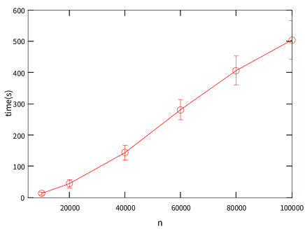
Figure 1: Execution time with random 3-SAT w.r.t. $n$ ($m=4.26n$)

We also conduct the second experiment to test the affinity of MatSat with GPU technology for large SAT problems with $n$ up to 300k. We reimplement MatSat using GPU (GeForce® GTX 1080 Ti) as MatSat-GPU and compare it with Sparrow2Riss-2018 which is the winner of Random Track in SAT competition 2018 [13] using large scale random SAT problems.

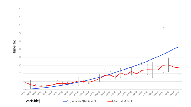
Figure 2: MatSat-GPU(red) and Sparrow2Riss-2018(blue) up to $n$ = 300k

In the experiment, as in the previous experiment, while varying $n$ from $n$ = $10k$ to $300k$ with $m=4.26\times n$, we run each solver 10 times on random SAT instances generated from different seeds and measure execution time. Average execution time by each solver is plotted in Figure 2(MatSat-GPU: red line, Sparrow2Riss-2018: blue line) with std (sample standard deviation). First, we can see that MatSat-GPU runs dozens of times faster than the CPU version of MatSat, depending on the number of variables, compared to the experiment in Figure 1. We also see that the average execution time by MatSat-GPU slowly rises w.r.t. $n$ until $n=300k$ while that of Sparrow2Riss-2018 rises more sharply. As a result, although Sparrow2Riss-2018 initially runs faster than MatSat-GPU, their curves cross around $n=170k$ and MatSat-GPU runs faster than Sparrow2Riss-2018 thereafter.

What is more conspicuous here is the difference in std, sample standard deviation. While the std of MatSat-GPU is rather stable through all $n$, Sparrow2Riss-2018 is not. Initially it has almost zero std but suddenly has a large std in $n$ = 270k and this happens again in $n$ = 290k and $n$ = 300k. The abrupt explosion of std seems to imply that for Sparrow2Riss-2018, most of generated random SAT instances are easily solvable but a very few of them are extraordinarily hard, causing abrupt explosion of std.

This experiment demonstrates the scalability of MatSat-GPU w.r.t. random 3-SAT and at the same time the affinity of MatSat’s matrix-based architecture for GPU. It additionally reveals the relative stability of the behavior of MatSat in SAT solving compared to Sparrow2Riss-2018 when dealing with large random 3-SAT.

0.5.2 Comparing MatSat with modern SAT solvers

Here we compare MatSat with the state-of-the-art SAT solvers. We consider four solvers from SAT competition 2018 [13, 12], i.e. Sparrow2Riss-2018 (Random Track, winner), gluHack (Random Track, ranked 2nd), glucose-3.0_PADC_10_NoDRUP (Random Track, ranked 3rd) and MapleLCMDistChronoBT (Main Track winner). We also consider MapleLCMDistChrBt-DL-v3 which is the winner of SAT RACE 2019 and a basic solver MiniSat 2.2 [9]. They are all CDCL solvers except for Sparrow2Riss-2018 which is a hybrid of SLS solver (Sparrow) and CDCL solver (Riss) [3]. We also compare MatSat with three SLS solvers. They are probSAT [2] which selects a varible based on a probability distribution, YalSAT [1] which is based on probSAT and the winner of 2017 SAT competition Random Track and CCAnr 1.1 [4] aiming at non-random SAT based on Configuration Checking with Aspiration (CCA) heuristics.

First we compare MatSat with these nine solvers by random SAT. We use three data sets: Set-A, Set-B and Set-C. Set-A contains 500 forced uniform random 3-SAT instances. Each instance is composed of $m=2130$ clauses in $n=500$ variables. Set-B is a random benchmark set taken from SAT competition 2018 [13, 12]. It consists of 55 random 3-SAT instances each of which contains $m$ clauses in $n$ variables where $n$ = 200$\sim$400 and $m$ = 4.3n. Set-C is a small set containing 10 random 5-SAT instances selected from a benchmark set submitted for SAT competition 2018 [13, 12]. Each instance is generated as “q-hidden formula” [15] with 5279 clauses in 250 variables and intended to be hard to SLS solvers.

Experimental settings are as follows. To run MatSat, we use max_itr = 500 and max_try = 100 for Set-A and Set-B and max_itr = 5000 and max_try = 2000 for Set-C. Set-A is divided into five sets of equal size and we run MatSat on each of five divided sets to obtain total execution time for 500 random 3-SAT instances. MatSat successfully returns a solution in all cases. For other solvers, default settings are used. timeout is set to 5000s and when it occurs it is counted as 5000s execution time. We measure average execution time per instance for Set-A and Set-C and the total execution time for Set-B.

Table 2: Execution time for random SAT

Solver	Data set
	Set-A	Set-B	Set-C
	time(s)*	time(s)	time(s)*	timeout/10
MatSat	0.0679	18.8	697.7	0/10
Sparrow2Riss-2018	0.0013	2.3	1544.1	3/10
gluHack	34.5	537.4	5000.0	10/10
glucose-3.0_PADC_10_NoDRUP	42.9	962.4	5000.0	10/10
MapleLCMDistChronoBT	0.34	519.1	5000.0	10/10
MapleLCMDistChronoBT_DL_v3	1.96	762.3	5000.0	10/10
MiniSat 2.2	3.28	50.1	5000.0	10/10
probSAT	0.0050	0.39	2134.8	2/10
YalSAT	0.0058	0.34	1018.6	1/10
CCAnr 1.1	0.0051	0.48	937.6	0/10

The experimental result is shown in Table 2 with best figures in bold face. Here time(s)* denotes execution time per instance. Set-C has the timeout column which denotes the number of occurrences of timeout in solving Set-C. We first observe that as far as Set-A and Set-B are concerned, in terms of execution time, pure CDCL solvers perform poorly while pure SLS solvers perform show their strength and the performance of MatSat is just between the two groups.

More interesting is the case of Set-C which is generated by the q-hidden method [15] so that the occurrence of literals in an instance is balanced, and hence more difficult than random SAT with unbalanced occurrences of literals. In the case of Set-C, all conventional solvers, CDCL or SLS type, cause timeout except for CCAnr 1.1. Even Sparrow2Riss-2018 which performs best for Set-A causes timeout three times. In particular, all pure CDCL solvers cause timeout for every instance. Consequently MatSat is ranked 1st on execution time of Set-C. We point out that MatSat outperforms all pure CDCL solvers. This observations is consistently understandable if we notice that MatSat bears some similarity to an SLS solver as explained in Section 0.4 and usually an SLS solver is good at solving random SAT.

To understand more deeply how MatSat can outperform these CDCL solvers, we examine the detail of a typical distribution of execution time in 100 forced random uniform 3-SAT instances by MatSat and three CDCL solvers (MiniSat 2.2, MapleLCMDistChronoBT and MapleLCMDistChronoBT_DL_v3) which is depicted in Figure 3.

Observe that MatSat, MapleLCMDistChronoBT and MapleLCMDistChronoBT_DL_v3 consume very similar time for instances numbered from about 30 to 100 but concerning the remaining instances, the latter two take much longer time than MatSat. In other words, about 30% of the 100 random SAT instances are extremely hard for the CDCL solvers while those instances are relatively easy for MatSat, which explains the superiority of average performance by MatSat compared to them. Also observe that the same phenomenon occurs between MatSat and MiniSat 2.2 where MiniSat 2.2 suddenly takes longer time for instances numbered less than 5. So we may say that the execution time by MatSat is more stable and less sensitive to the difference in individual instances compared to other solvers. This stability could be ascribed to the global nature of MatSat’s update scheme (3) which always takes all components in a candidate assignment into account unlike the sequential discrete update (with almost inevitable backtracking) on components in the candidate assignment made by a CDCL solver.

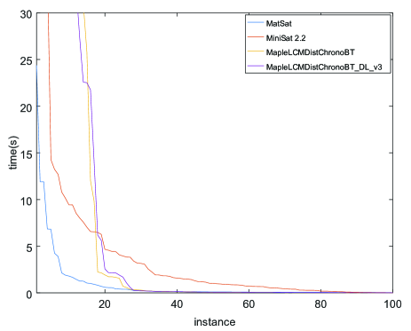
Figure 3: Distribution of execution time for 100 instances (n=500,m=2130)

So far we have been focusing solely on random SAT instances which have different characteristics from non-random ones. So we additionally conduct an experiment to compare ten solvers by non-random (structured) SAT.

We prepare three benchmarks. The first one is Set-D taken from SATLIB [14]. It contains 100 satisfiable 3-SAT instances where each instance has $m=300$ clauses in $n=90$ variables. The second one is Set-E also taken from SATLIB [14]. It contains 100 satisfiable 5-SAT instances where each instance has $m=3100$ clauses in $n=500$ variables. The third one is Set-F from SAT competition 2018 Main Track [13, 12] submitted by Chen [5], which encodes relativized pigeonhole principle (RPHP) [7] and contains 20 satisfiable 3-SAT instances where each instance has $m=1120$ clauses in $n=320$ variables (concerning Set-F, it was initially assumed to be non-random SAT but later we are informed by reviewers that Chen’s benchmarks are not non-random and Set-F should be counted as a random SAT problem. We are sorry that we were not aware of the random nature of Set-F. So the result with Set-F should be taken as showing the behavior of MatSat with random SAT like problems).

We run ten solvers, i.e., MatSat, Sparrow2Riss-2018, gluHack, glucose-3.0_PADC_10_NoDRUP, MapleLCMDistChronoBT, MapleLCMDistChronoBT_DL_v3, MiniSat 2.2, probSAT, YalSAT and CCAnr 1.1. Their experimental settings are as follows. To run MatSat, we use max_itr = 500 and max_try = 100 for Set-D, max_itr = 2000 and max_try = 100 for Set-E and max_itr = 500 and max_try = 1000 for Set-F. Given these parameters, MatSat successfully finds a solution for all instances. For other solvers, default settings are used. timeout is set to 5000s. When timeout occurs, we equate execution time to 5000s. We measure the total execution time for Set-D and Set-E, and average execution time per instance for Set-F.

Table 3: Execution time for non-random and random SAT

Solver	Data set
	Set-D	Set-E	Set-F
	time(s)	time(s)	time(s)*	timeout/20
MatSat	9.29	679.7	2.0	0/20
Sparrow2Riss-2018	0.23	0.26	251.9	1/20
gluHack	0.32	0.58	5000.0	20/20
glucose-3.0_PADC_10_NoDRUP	0.45	0.63	4346.2	17/20
MapleLCMDistChronoBT	0.22	0.42	3643.7	12/20
MapleLCMDistChronoBT_DL_v3	0.24	0.42	3205.7	10/20
MiniSat 2.2	0.21	0.21	4345.8	15/20
probSAT	0.46	0.46	14.3	0/20
YalSAT	0.39	0.45	41.3	0/20
CCAnr1.1	0.39	0.50	14.2	0/20

Table 3 shows the result with best figures in bold face. time(s)* in the table denotes execution time per instance. Set-F has the timeout column which denotes the number of occurrences of timeout in solving 20 instances in Set-F.

MatSat performs very poorly on Set-D and Set-E compared to other solvers. However, Set-F shows quite different performance (as mentioned before, Set-F should be considered as a random SAT problem). As the timeout column in Table 3 tells, MatSat and three SLS solvers (probSAT, YalSAT, CCAnr 1.1) causes no timeout, but Sparrow2Riss-2018 causes timeout once and other four CDCL solvers cause timeout ten times or more. Also while none of the SLS solvers causes timeout, they take much longer time than MatSat to solve Set-F. As a reuslt, MatSat outperforms all nine solvers that participate in the experiment.

Although we cannot stretch experimental results in this section too far, we may say that MatSat behaves differently in SAT solving from existing SAT solvers, sometimes giving an advantage in the case of random SAT.

0.6 Weighted variables and clauses

The experimental results in the previous section uncover poor performance of MatSat on non-random SAT. We here propose to introduce weighted variables and clauses to improve the situation. The idea is to introduce a real number, variable weight, for each variable to tell the solver which variable is important. Also we introduce a real number, clause weight, for each clause. Those variables and clauses that have large weights have the priority to be optimized by the solver just like unit clauses are specially treated by unit propagation.

More formally, when an instance matrix ${\mathbf{Q}}(m\times 2n)$ is given, we introduce a variable weight vector ${\mathbf{w}}_{v}(1\times n)$ and a clause weight vector ${\mathbf{w}}_{c}(m\times 1)$ w.r.t. ${\mathbf{Q}}$. Let $a_{i}$ $(1\leq i\leq n)$ be the $i$-th variable and ${\mathbf{w}}_{v}^{*}(i)$, the $i$-th element of ${\mathbf{w}}_{v}^{*}$, be the number of total occurrences of $a_{i}$ in the SAT instance represented by ${\mathbf{Q}}$. We define the variable weight ${\mathbf{w}}_{v}(i)$ for $a_{i}$ as ${\mathbf{w}}_{v}(i)={\mathbf{w}}_{v}^{*}(i)/{\rm ave}({\mathbf{w}}_{v}^{*})$ where ${\rm ave}({\mathbf{w}}_{v}^{*})$ is the average of elements in ${\mathbf{w}}_{v}^{*}$. We next define a clause weight ${\mathbf{w}}_{c}(j)$ $(1\leq j\leq m)$ for the $j$-th clause $C_{j}$ represented by the $j$-th row of ${\mathbf{Q}}$ as the sum of weights of variables in $C_{j}$. Finally we define ${\rm J}^{sat\_w}$, a weighted version of ${\rm J}^{sat}$, by

$${\rm J}^{sat\_w} = ({\mathbf{1}}_{m}\bullet({\mathbf{w}}_{c}\odot({\mathbf{1}}_{m}-\mbox{min}_{1}({\mathbf{Q}}\tilde{\mathbf{u}}^{d}))))+(\ell/2)\cdot\|{\mathbf{w}}_{v}^{T}\odot\tilde{\mathbf{u}}\odot({\mathbf{1}}_{n}-\tilde{\mathbf{u}})\|_{2}^{2}.$$ (4)

Since $({\mathbf{1}}_{m}-\mbox{min}_{1}({\mathbf{Q}}\tilde{\mathbf{u}}^{d}))(j)$ is the falsity of the $j$-th clause $C_{j}$, being multiplied by a large weight ${\mathbf{w}}_{c}(j)$ in ${\rm J}^{sat\_w}$ means the continuous falsity of $C_{j}$ is more strongly minimized than other clauses in learning. Put ${\mathbf{Q}}=[{\mathbf{Q}}_{1}\,{\mathbf{Q}}_{2}]$ where ${\mathbf{Q}}_{1}$ (resp. ${\mathbf{Q}}_{2}$) represents the positive literals (resp. negative literals) of ${\mathbf{Q}}$. Then ${\rm J}^{sat\_w}$’s Jacobian ${\mathbf{J}}_{acb}^{sat\_w}$ is computed as follows (derivation omitted).

$${\mathbf{J}}_{acb}^{sat\_w} = ({\mathbf{Q}}_{2}-{\mathbf{Q}}_{1})^{T}({\mathbf{w}}_{c}\odot[({\mathbf{Q}}\tilde{\mathbf{u}}^{d})\leq{\mathbf{1}}_{m}])+\ell\cdot({\mathbf{w}}_{v}^{T}\odot{\mathbf{w}}_{v}^{T}\odot\tilde{\mathbf{u}}\odot({\mathbf{1}}_{n}-\tilde{\mathbf{u}})\odot({\mathbf{1}}_{n}-2\tilde{\mathbf{u}}))$$ (5)

We conduct a small experiment on non-random SAT using this weighted version of MatSat. It minimizes ${\rm J}^{sat\_w}$ (4) by Newton’s method using (5). In addition to Set-E and Set-F, we use another test set Set-G from SATLIB [14] in the experiment containing 100 instances of 5-SAT with $m=3100$ clauses in $n=500$ variables. The experimental result is summarized in Table 4.

Table 4: Learning time(s) by the weighted and non-weighted MatSat on non-random SAT instances

MatSat	Set-D	Set-E	Set-G
non-weighted	9.29	679.7	1277.3
(max_itr max_try)	(500 100)	(2k 100)	(5k 100)
weighted	2.18	82.4	123.7
(max_itr max_try)	(100,300)	(1k,100)	(200,100)

Comparing the non-weighted version and the weighted version, we notice that the weighted MatSat learns much faster, almost an order of magnitude faster for Set-G, than the non-weighted MatSat, with a small number of iterations. Although this experiment is small, it attests the effectiveness of weighted variables and clauses for MatSat to control the learning process and suggests one way to improve the performance of MatSat on non-random SAT.

0.7 Related Work

SAT is a central discipline of computer science and the primary purpose of this paper is to bring a differentiable approach into this established field from the viewpoint of integrating symbolic reasoning and numerical computation. But, first, we put our work in the traditional context.

According to a comprehensive survey [11], our proposal is categorized as continuous-unconstrained global optimization approach. We note that a variety of global optimization approaches are described in [11] but all encode clauses as a product of some literal functions as in [10]. As a result, the objective function for $n$ variables becomes a multivariate polynomial of degree possibly up to $2n$. Contrastingly in our approach, clauses are not functions but constant vectors collectively encoding a SAT instance as an instance matrix, and far more importantly, our objective function is not a simple multivariate polynomial but a sum of two terms with distinct roles as explained next. First recall our objective function ${\rm J}^{sat}$ is of the form: ${\rm J}^{sat}=f+r$ where $f=({\mathbf{1}}_{m}\bullet({\mathbf{1}}_{m}-\mbox{min}_{1}({\mathbf{Q}}\tilde{\mathbf{u}}^{d})))$ using $\mbox{min}_{1}(x)$and $r=(\ell/2)\cdot\|\tilde{\mathbf{u}}\odot({\mathbf{1}}_{n}-\tilde{\mathbf{u}})\|_{2}^{2}$. While $r$ is just a multivariate polynomial of constant degree, four, working as a penalty term to force 0-1 vectors, $f$ is essential and navigates SAT solution search as a continuous surrogate of the number of false clauses. Unlike various UniSAT models in [11], it is not a product of functions but a sum of piecewise linear functions of $\tilde{\mathbf{u}}$, which makes all the difference from the viewpoint of optimization. In particular, when all components of ${\mathbf{Q}}\tilde{\mathbf{u}}^{d}$ are less than one, it becomes linear w.r.t. $\tilde{\mathbf{u}}$. So when $\tilde{\mathbf{u}}$ is distant from a solution and ${\mathbf{Q}}\tilde{\mathbf{u}}^{d}$ which is a continuous approximation to the number of true literals in clauses is small, the convergence of $f$ is likely to be fast due to the linearity of $f$.

Now we focus on related works from the viewpoint of of integrating symbolic reasoning and numerical computation. As explained Section 0.1, there has been a steady stream of tensorizing logic programming [23, 24, 22, 17, 26] in which for example, Sato experimentally implemented a differentiable SAT solver in Octave and compared its performance with one CDCL solver [26].

There is also a trend of combining neural computation with logic programming. For example, DeepProbLog allows the user to write “neural predicates” computed by a neural network and the probability of a query is computed just like usual ProbLog programs while using probabilities computed by the neural predicates [18]. T-PRISM replaces the basic data structure with tensor computation in a logic-based probabilistic modeling language PRISM [25] and makes it possible to learn neural networks [17].

Direct attempts at a differentiable SAT solver include the work done by Nickles that integrates the derivative of a loss function with a traditional SAT solver [19]. Wang shows that a MAXSAT can be incorporated into a convolutional neural network to realize end-to-end learning of visual Sudoku problems [28]. Selsam et al.’s neural net classifier NeuroSAT achieves 85% classification accuracy on moderate size problems with 40 variables and could extract solutions 70% of satisfiable cases [27].

Last but not least, there are some works on the use of GPU, for example, for simplification [20] and for CDCL solvers [21]. In the latter case, Osama et al.  used GPU for inprocessing such as garbage collection and simplification.

0.8 Conclusion

We proposed a simple differentiable SAT solver MatSat. It is a new type of SAT solver, not a CDCL solver or an SLS solver. It carries out SAT solving in vector spaces as cost minimization of a cost function ${\rm J}^{sat}(\tilde{\mathbf{u}})$ w.r.t.  a continuous assignment $\tilde{\mathbf{u}}$ applied to a binary matrix ${\mathbf{Q}}$ representing a SAT instance. We empirically confirmed the scalability of MatSat. In particular, it is shown that when implemented by GPU, it can solve random 3-SAT instances of various sizes up to $n=3\times 10^{5}$ variables. We then compared MatSat with nine modern SAT solvers including representative CDCL and SLS solvers in terms of execution time. When applied to three data sets of random SAT instances, it outperforms all CDCL solvers but is outperformed by all SLS solvers for two easy sets. On the other hand concerning the data set designed to be hard for SLS solvers, it outperforms all nine solvers. We also conducted a comparative experiment with non-random SAT sets and discovered that MatSat performs poorly on these sets. Apparently the number of experiments is not enough but these results seem to suggest the unique behavior of MatSat different from SLS and CDCL solvers.

As future work, we need to conduct more experiments with various types of SAT instances including (unforced) uniform random k-SAT instances and structured ones. It is our plan to improve GPU implementation and introduce heuristics for parameters $\ell$ in (1) and $\beta$ in Algorithm 1. We also plan to reconstruct MatSat for MAXSAT, which seems straightforward because ${\mathbf{v}}=\mbox{min}_{1}({\mathbf{Q}}{\mathbf{u}}^{d})$ in ${\rm J}^{sat}$ computed by MatSat is actually an indicator vector of clauses satisfied by an assignment vector ${\mathbf{u}}$ and $\|{\mathbf{v}}\|_{1}$ is the number of satisfied clauses. Hence by relaxing ${\mathbf{u}}$ to $\tilde{\mathbf{u}}\in\mathbb{R}^{n}$ and concurrently relaxing ${\mathbf{v}}$ to $\tilde{\mathbf{v}}\in\mathbb{R}^{n}$, we would have a differentiable formulation of MAXSAT that optimizes $\|\tilde{\mathbf{v}}\|_{1}$.

MatSat is at the cross-roads of SAT solving, machine learning and (propositional) logic and also closely related to neural networks. It is an instance of differentiable approaches emerging in various fields ranging from neural networks to logic programming that solve symbolic problems in a differentiable framework in a continuous space. We expect that MatSat opens a new approach to building a powerful GPU-based SAT solver.

References

- [1] Andreas Fröhlich Uwe Schöning Adrian Balint, Armin Biere. Improving implementation of sls solvers for sat and new heuristics for k-sat with long clauses. In In: Sinz C., Egly U. (eds) Theory and Applications of Satisfiability Testing – SAT 2014, LNCS Volume 8561.
- [2] Uwe Schöning Adrian Balint. Choosing probability distributions for stochastic local search and the role of make versus break. In In: Cimatti A., Sebastiani R. (eds) Theory and Applications of Satisfiability Testing – SAT 2012, LNCS Volume 7317.
- [3] Adrian Balint and Norbert Manthey. Sparrowtoriss. In Anton Belov, Daniel Diepold, Marijn J.H. Heule, and Matti Järvisalo, editors, Proceedings of SAT Competition 2014, volume B-2014-2 of Department of Computer Science Series of Publications B, page 77. University of Helsinki, Helsinki, Finland, 2014.
- [4] Su K. Cai S., Luo C. A configuration checking based local search solver for non-random satisfiability. In In: Heule M., Weaver S. (eds) Theory and Applications of Satisfiability Testing – SAT 2015, LNCS Volume 9340.
- [5] Jingchao Chen. Encodings of relativized pigeonhole principle formulas with auxiliary constraints. In Proceedings of SAT Competition 2018 : Solver and Benchmark Descriptions, Department of Computer Science Series of Publications B, vol. B-2018-1, page 63. Department of Computer Science, University of Helsinki, 2018.
- [6] Nuri Cingillioglu and Alessandra Russo. DeepLogic: End-to-End Logical Reasoning. CoRR, abs/1805.07433, 2018.
- [7] Jan Elffers, Jesús Giráldez-Cru, Stephan Gocht, Jakob Nordström, and Laurent Simon. Seeking practical cdcl insights from theoretical sat benchmarks. In Proceedings of the Twenty-Seventh International Joint Conference on Artificial Intelligence, IJCAI-18, pages 1300–1308. International Joint Conferences on Artificial Intelligence Organization, 2018.
- [8] Richard Evans and Edward Grefenstette. Learning explanatory rules from noisy data. J. Artif. Intell. Res., 61:1–64, 2018.
- [9] Niklas Eén and Niklas Sörensson. An extensible sat-solver. In Enrico Giunchiglia and Armando Tacchella, editors, SAT, volume 2919 of Lecture Notes in Computer Science, pages 502–518. Springer, 2003.
- [10] Jun Gu, Qian-Ping Gu, and Ding-Zhu Du. Convergence properties of optimization algorithms for the sat problem. 45(2):209–219, 1996.
- [11] Jun Gu, Paul W. Purdom, John Franco, and Benjamin W. Wah. Algorithms for the satisfiability (sat) problem: A survey. In DIMACS Series in Discrete Mathematics and Theoretical Computer Science, pages 19–152. American Mathematical Society, 1996.
- [12] Marijn Heule, Matti Järvisalo, and Martin Suda. Sat competition 2018. Journal on Satisfiability, Boolean Modeling and Computation, 11(1):133–154, 2019.
- [13] Marijn J. H. Heule, Matti Juhani Järvisalo, and Martin Suda, editors. Proceedings of SAT Competition 2018: Solver and Benchmark Descriptions, volume B-2018-1 of Department of Computer Science Series of Publications B. Department of Computer Science, University of Helsinki, 2018.
- [14] Holger H. Hoos and Thomas Stützle. An online resource for research on sat. In T.Walsh I.P.Gent, H.v.Maaren, editor, Proceedings of SAT Competition 2000, pages 283–292. IOS Press, 2000.
- [15] Haixia Jia, Cristopher Moore, and Doug Strain. Generating hard satisfiable formulas by hiding solutions deceptively. In Manuela M. Veloso and Subbarao Kambhampati, editors, Proceedings of The Twentieth National Conference on Artificial Intelligence and the Seventeenth Innovative Applications of Artificial Intelligence Conference, pages 384–389. AAAI Press / The MIT Press, 2005.
- [16] Diederik P. Kingma and Jimmy Ba. Adam: A method for stochastic optimization. In Yoshua Bengio and Yann LeCun, editors, 3rd International Conference on Learning Representations, ICLR 2015, San Diego, CA, USA, May 7-9, 2015, Conference Track Proceedings, 2015.
- [17] Ryosuke Kojima and Taisuke Sato. T-PRISM: A tensorized logic programming language for large-scale data. In Proceedings of the 14th International workshop on Neural-Symbolic Learning and Reasoning (NeSy’19), 2019.
- [18] Robin Manhaeve, Sebastijan Dumancic, Angelika Kimmig, Thomas Demeester, and Luc De Raedt. Deepproblog: Neural probabilistic logic programming. CoRR, 2018.
- [19] Matthias Nickles. Sampling-based SAT/ASP multi-model optimization as a framework for probabilistic inference. In Proceedings of the 28th International Conference,ILP 2018, pages 88–104, 2018.
- [20] Muhammad Osama and Anton Wijs. Parallel sat simplification on gpu architectures. In Tomáš Vojnar and Lijun Zhang, editors, Tools and Algorithms for the Construction and Analysis of Systems, pages 21–40. Springer International Publishing, 2019.
- [21] Muhammad Osama, Anton Wijs, and Armin Biere. SAT solving with GPU accelerated inprocessing. In Jan Friso Groote and Kim Guldstrand Larsen, editors, Tools and Algorithms for the Construction and Analysis of Systems - 27th International Conference, TACAS 2021, Held as Part of the European Joint Conferences on Theory and Practice of Software, ETAPS 2021, Luxembourg City, Luxembourg, March 27 - April 1, 2021, Proceedings, Part I, volume 12651 of Lecture Notes in Computer Science, pages 133–151. Springer, 2021.
- [22] Chiaki Sakama, Hien Nguyen, Taisuke Sato, and Katsumi Inoue. Partial evaluation of logic programs in vector spaces. In Proceedings of the 11th Workshop on Answer Set Programming and Other Computing Paradigms (ASPOCP 2018), 2018.
- [23] Taisuke Sato. A linear algebraic approach to Datalog evaluation. Theory and Practice of Logic Programming (TPLP), 17(3):244–265, 2017.
- [24] Taisuke Sato, Katsumi Inoue, and Chiaki Sakama. Abducing relations in continuous spaces. In Proceedings of the 27th International Joint Conference on Artificial Intelligence (IJCAI-ECAI-18), pages 1956–1962, 2018.
- [25] Taisuke Sato and Yoshitaka Kameya. Parameter learning of logic programs for symbolic-statistical modeling. Journal of Artificial Intelligence Research, 15:391–454, 2001.
- [26] Taisuke Sato and Ryosuke Kojima. Logical inference as cost minimization in vector spaces. In Artificial Intelligence IJCAI 2019 International Workshops, Revised Selected Best Papers (Amal El Fallah Seghrouchni,David Sarne (Eds.)), pages 239–252. 2020.
- [27] Daniel Selsam, Matthew Lamm, Benedikt Bünz, Percy Liang, Leonardo de Moura, and David L. Dill. Learning a SAT solver from single-bit supervision. In International Conference on Learning Representations (ICLR’19), 2019.
- [28] Po-Wei Wang, Priya L. Donti, Bryan Wilder, and J. Zico Kolter. Satnet: Bridging deep learning and logical reasoning using a differentiable satisfiability solver. In Proceedings of the 36th International Conference on Machine Learning (ICML 2019), California, USA, pages 6545–6554, 2019.
- [29] Po-Wei Wang and J. Zico Kolter. Low-rank semidefinite programming for the MAX2SAT problem. In The Thirty-Third AAAI Conference on Artificial Intelligence (AAAI 2019), Hawaii, USA, pages 1641–1649, 2019.