Are all outliers alike?
A Taxonomy of Out of Distribution Samples

Ramneet Kaur Susmit Jha Anirban Roy Sangdon Park Oleg Sokolsky Insup Lee Ramneet Kaur , Susmit Jha , Anirban Roy^†^†footnotemark: , Sangdon Park, Oleg Sokolsky^†^†footnotemark: , & Insup Lee^†^†footnotemark:
ramneetk@seas.upenn.edu,{susmit.jha,anirban.roy}@sri.com,
{sangdonp, sokolsky, lee}@cis.upenn.edu Ramneet Kaur is a graduate student at the Department of Computer and Information Science, University of Pennsylvania, Philadelphia, USA. This work was done when she was a summer intern at SRI.Computer Science Laboratory, SRI International, Menlo Park, CA 94025, USADepartment of Computer and Information Science, University of Pennsylvania, Philadelphia, USA.

Are all outliers alike?
On Understanding the Diversity of Outliers
for Detecting OODs

Detecting OODs as datapoints with High Uncertainty

Abstract

Deep neural networks (DNNs) are known to produce incorrect predictions with very high confidence on out-of-distribution inputs (OODs). This limitation is one of the key challenges in the adoption of DNNs in high-assurance systems such as autonomous driving, air traffic management, and medical diagnosis. This challenge has received significant attention recently, and several techniques have been developed to detect inputs where the model’s prediction cannot be trusted. These techniques detect OODs as datapoints with either high epistemic uncertainty or high aleatoric uncertainty. We demonstrate the difference in the detection ability of these techniques and propose an ensemble approach for detection of OODs as datapoints with high uncertainty (epistemic or aleatoric). We perform experiments on vision datasets with multiple DNN architectures, achieving state-of-the-art results in most cases.

Machine Learning, ICML

1 Introduction

DNNs have achieved remarkable performance in many areas such as computer vision (Gkioxari et al., 2015), speech recognition (Hannun et al., 2014), and text analysis (Majumder et al., 2017). But their deployment in the safety-critical systems such as self-driving vehicles (Bojarski et al., 2016), medical diagnoses (De Fauw et al., 2018) is hindered by their brittleness. One major challenge is the inability of DNNs to be self-aware of when new inputs are outside the training distribution and likely to produce incorrect predictions. It has been widely reported in literature (Guo et al., 2017; Hendrycks & Gimpel, 2016) that DNNs exhibit overconfident incorrect predictions on inputs which are outside the training distribution. The responsible deployment of DNNs in high-assurance applications necessitates detection of out-of-distribution datapoints (OODs) so that DNNs can abstain from making decisions on those.

OODs are those points that do not belong to any class of the in-distribution (iD). Existing techniques detect OODs as datapoints that have either lack of support from the iD data (Lee et al., 2018; An & Cho, 2015) or high entropy in the class prediction (Hendrycks & Gimpel, 2016; Steinhardt & Liang, 2016). Lack of support from the iD data indicates high epistemic uncertainty (EU) and high entropy in the class prediction indicates high aleatoric uncertainty (Hüllermeier & Waegeman, 2019). Existing techniques can thus be classified into two categories; one that detect OODs due to high EU and other that detect OODs due to high AU. We propose detecting OODs as datapoints with high uncertainty (aleatoric or epistemic).

High entropy in the predictive distribution by the ensemble of classifiers has been proposed by Lakshminarayanan et al. (2016) for OOD detection. We propose OOD detection with an ensemble of detectors where each detector is composed of indicators for both, high EU and high AU.

We make the following three contributions in this paper:

•

Classification of OOD detection techniques. We classify the existing techniques as detecting OODs due to either high EU or high AU.
•

OODs as datapoints with high uncertainty. We illustrate difference in the detection abilities of the classified techniques and propose detecting OODs as datapoints with high uncertainty (aleatoric or epistemic).
•

Ensemble approach to detect OODs. We propose a novel OOD detection technique based on the ensemble of OOD detectors where each detector is composed of indicators for both, high EU and high AU.
•

Empirical evaluation. We demonstrate the effectiveness of our approach on several vision benchmarks, obtaining state-of-the-art (SOTA) results.

2 Background

OOD datapoints (OODs) do not belong to (any class of) the in-distribution (iD). So, OODs can be detected by:

1.

Lack of support (or evidence) from the iD data to make decision on these points as they do not belong to the iD; indicating high epistemic uncertainty (EU) (Hüllermeier & Waegeman, 2019).
2.

High entropy in the class prediction as they do not belong to any iD class; indicating high aleatoric uncertainty (AU) (Hüllermeier & Waegeman, 2019).

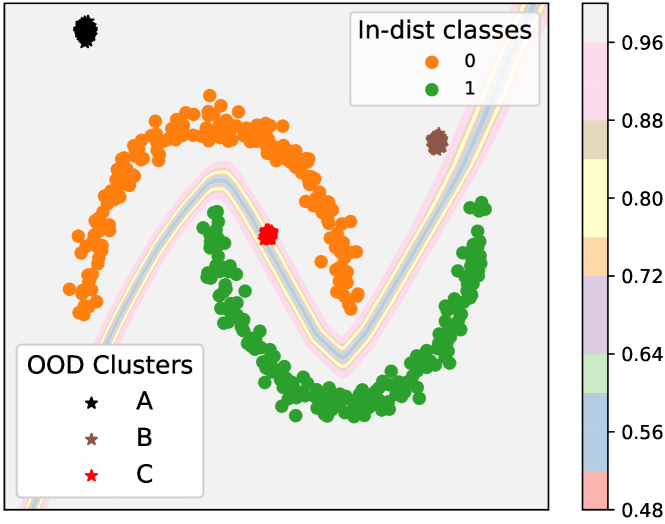
Existing OOD detection techniques. Current approaches for OOD detection detect OODs as datapoints either with high EU or high AU. Therefore, they differ in their ability to detect OODs. We demonstrate this difference on a 2D half-moon dataset. As shown in Figure 1, we consider three clusters of OODs: cluster $A$ (black), $B$ (brown) and $C$ (red).

Refer to caption — Figure 1: (Left) shows the 2 iD half-moon classes, 3 OOD clusters, and the trained classifier’s boundary with softmax scores in the input space. (Right) shows iD samples and OODs in the classifier’s penultimate feature space.

We consider two approaches for detecting OODs with EU and two approaches for detecting OODs with high AU:

•

Lee et al. (2018) propose using Mahalanobis distance of an input from the iD density for OOD detection. This corresponds to using lack of support from the iD data, i.e., large distance from the iD density to detect OODs as datapoints with high EU. Figure 2(a) shows that the Mahalanobis distance from the mean and covariance of all the iD data in the penultimate feature space is only able to detect the cluster $A$ that lie far from the iD density.
•

Using reconstruction error from the Principal Component Analysis (PCA) (Hoffmann, 2007) on the iD data is another approach that detects OODs as data points with high EU. This is because it uses lack of support from the iD data, i.e., high reconstruction error from the PCA of the iD data for OOD detection. Figure 2(b) shows that using minimum reconstruction error from the class-conditional PCA performed in the feature space of the iD data is able to detect OODs from clusters $A$ and $B$ .
•

Hendrycks & Gimpel (2016) propose using maximum softmax probability as an indicator of the KL-divergence between distribution of the predicted softmax probabilities and the uniform distribution. This divergence measures entropy in the prediction of the class for an input (Steinhardt & Liang, 2016) and therefore detects OODs as data points with high AU. Figure 2(c) shows that this technique (SBP) is able to detect those OODs that lie on or near the decision boundary where the classifier is least confident or has high entropy in its prediction.
•

Another approach for detection of OODs as data points with high AU is by using non-conformance in the labels of the K-Nearest Neighbors for OOD detection (DkNN) (Papernot & McDaniel, 2018). As shown in Figure 2(d), entropy in the label of the kNNs from the penultimate layer is only able to detect OODs with nearest neighbors from multiple classes (cluster $C$ ).

Existing techniques for detecting OODs due to either high AU or high EU are summarized in Table 2 of appendix.

Proposed approach for OOD detection. We propose using both lack of support from the iD data as well as high entropy in the class prediction to detect OODs as datapoints with high uncertainty (epistemic or aleatoric). Further, as observed from the toy example, techniques for detecting OODs as datapoints with high EU (or AU) such as Mahalanobis and PCA (or SBP and DkNN) also differ in their abilities. Therefore, we propose using an ensemble of OOD detectors where each detector is composed of indicators for both, high EU and high AU. Figure 3 shows improvement in the True Negative Rate (TNR) of the proposed technique with two detectors over a single detector on the two half-moons dataset.¹¹1Empirical evaluation on CIFAR10 and SVHN in appendix A.3.3 also justify these observations. We compare the performance of ensemble approach with the indicators of high AU and high EU as well as individual detectors used in the ensemble approach. Our approach achieves SOTA in almost all cases.

3 Ensemble approach for detection of OODs as datapoints with high uncertainty

OODs as datapoints with high AU. For a given threshold $\delta_{a}$ on the entropy in the predicted class distribution for the iD data and $n_{c}$ as the number of classes, an input $x$ is detected as an OOD due to high AU if $-\sum\limits_{i=1}^{n_{c}}p_{i|x}\ \log\ (p_{i|x})>\delta_{a}.$ Here $p_{i|x}$ is the predicted probability of $x$ in class $i$ .

OODs as datapoints with high EU. Probability density function (PDF) estimated from the iD data can be used to provide support for a datapoint belonging to the iD. For a given threshold $\delta_{e}$ on the probability of an input $x$ belonging to the iD density and $\{q_{i}(.)\ :\ 1\leq i\leq n_{c}\}$ as the class-conditional iD PDF set, $x$ is detected as an OOD due to high EU if $\displaystyle\max_{i=1}^{n_{c}}\{q_{i}(x)\}<\delta_{e}.$

OODs as data points with high uncertainty. We detect an input $x$ as an OOD if it has high AU or high EU:

-\sum\limits_{i=1}^{n_{c}}p_{i|x}\ \log\ (p_{i|x})>\delta_{a}\vee\displaystyle\max_{i=1}^{n_{c}}\{q_{i}(x)\}<\delta_{e}.

(1)

There are different ways of assigning score to the OOD nature of an input $x$ from (1). We call these scores as uncertainty scores. One way to compute the uncertainty score is by picking the dominating uncertainty:

\displaystyle\max(-\sum_{i=1}^{n_{c}}p_{i|x}\ \log\ (p_{i|x})-\delta_{a},\delta_{e}-\max_{i=1}^{n_{c}}\{q_{i}(x)\})

(2)

Another way is to use the linear combination of AU and EU:

	$\displaystyle w_{1}\times(-\sum\limits_{i=1}^{n_{c}}p_{i\|x}\ \log\ (p_{i\|x}))$		(3)
	$\displaystyle+\ w_{2}\times(\displaystyle\max_{i=1}^{n_{c}}\{q_{i}(x)\})$

There can be other ways of assigning uncertainty score to the input. We use the score from (3) in our experiments.

Ensemble approach for OOD detection. We propose OOD detection by combining uncertainty scores by different detectors. There are multiple ways of assigning weights to the predictions of individual detectors in an ensemble approach (Dietterich, 2000). We use logistic regression for assigning weights to the uncertainty scores by individual detectors in our experiments.

4 Experimental Results

Individual detectors. We use two detectors in the proposed ensemble approach for OOD detection. First detector is composed of the Mahalanobis distance (for EU)²²2Mahalanobis distance of an input from the estimated iD density corresponds to measuring the log of probability densities of an input (Lee et al., 2018). Using mahalanobis distance from the empirical class means and tied empirical covariance of all the training iD data thus detects OODs as datapoints with high EU. and ODIN (Liang et al., 2017) with $\epsilon=0.005$ and $T=10$ (for AU). Second detector is composed of the minimum reconstruction error from the class-conditional PCA on the top 40% eigen vectors (for EU)³³3PCA can be viewed as a maximum likelihood procedure on a Gaussian density model of the observed data (Tipping & Bishop, 1999). Performing class-wise reconstruction error from PCA thus detects OODs as datapoints with high EU. and a novel non-conformance measure amongst nearest neighbors⁴⁴4Details are given in the appendix. (for AU).

Evaluation. We evaluate the proposed technique on different iD datasets on different architectures. We consider MNIST (LeCun et al., 1998), CIFAR10 (Krizhevsky et al., 2009) and SVHN (Netzer et al., 2011) as iD datasets. KMNIST (Clanuwat et al., 2018) and F-MNIST (Xiao et al., 2017) datasets are considered as OOD for MNIST. For CIFAR10 and SVHN, we consider LSUN (Yu et al., 2015), Imagenet (Deng et al., 2009), SVHN (for CIFAR10 as iD) and CIFAR10 (for SVHN as iD) as OOD. We also consider a Subset-CIFAR100 as OODs for CIFAR10 and SVHN. Specifically, from the CIFAR100 classes, we select sea, road, bee, and butterfly as OOD which are visually similar (and thus challenging OOD for CIFAR10) to the ship, automobile, and bird classes in the CIFAR10, respectively. We report TNR at 95% TPR, area under receiver operating characteristic curve (AUROC), and detection accuracy (DTACC). We compare with the SOTA detectors that are used as indicators of AU or EU in our approach; namely SBP (Hendrycks & Gimpel, 2016), ODIN (Liang et al., 2017) and Mahalanobis (Lee et al., 2018).

Results. Table 1 shows that the proposed ensemble approach for detecting OODs as datapoints with high uncertainty outperforms SOTA in almost all the cases. Figure 4 shows the t-SNE (Maaten & Hinton, 2008) plot of the penultimate features from the ResNet50 model trained on CIFAR10. We show 4 examples of OODs (2 due to high EU and 2 due to high AU) from Subset-CIFAR100. These OODs were detected by the proposed approach but missed by the Mahalanobis approach.

Table 1: Comparison with SBP, ODIN and Mahalanobis as SOTA OOD detection techniques.

MNIST (LeNet5) TNR (95% TPR) AUROC DTACC $D_{out}$ SBP ODIN Mahala Ours SBP ODIN Mahala Ours SBP ODIN Mahala Ours KMNIST 69.33 67.72 80.52 91.7 93.24 92.98 96.53 98.29 86.88 85.99 90.82 93.98 F-MNIST 52.69 58.47 63.33 72.62 89.19 90.76 94.11 95.49 82.77 83.21 87.76 90.56 CIFAR-10 (ResNet34) TNR (95% TPR) AUROC DTACC $D_{out}$ SBP ODIN Mahala Ours SBP ODIN Mahala Ours SBP ODIN Mahala Ours SVHN 32.47 72.85 53.16 83.2 89.88 93.85 93.85 96.91 85.06 85.40 89.17 91.16 LSUN 45.44 45.16 77.53 81.23 91.04 89.63 96.51 96.87 85.26 81.83 90.64 91.19 ImageNet 44.72 46.54 68.41 74.53 91.02 90.45 95.02 95.73 85.05 83.06 88.63 89.73 SCIFAR100 38.17 37.00 38.39 51.11 88.91 86.13 88.86 93.85 82.34 78.50 82.51 89.93 CIFAR-10 (ResNet50) TNR (95% TPR) AUROC DTACC $D_{out}$ SBP ODIN Mahala Ours SBP ODIN Mahala Ours SBP ODIN Mahala Ours SVHN 44.69 86.61 34.49 88.8 97.31 84.41 98.19 97.84 86.36 91.25 76.72 92.26 LSUN 48.37 80.72 32.18 81.38 92.78 96.51 87.09 96.93 86.97 90.59 80.07 91.79 ImageNet 42.06 73.23 29.48 74.44 90.80 94.91 84.30 95.6 84.36 88.23 77.19 89.42 SCIFAR100 36.39 47.44 21.06 48.33 89.09 86.16 77.42 92.98 83.37 78.69 71.43 88.27 CIFAR-10 (DenseNet) TNR (95% TPR) AUROC DTACC $D_{out}$ SBP ODIN Mahala Ours SBP ODIN Mahala Ours SBP ODIN Mahala Ours SVHN 39.22 69.96 83.63 90.92 88.24 92.02 97.10 98.41 82.41 84.10 91.26 93.29 LSUN 48.38 71.89 46.63 83.47 92.14 94.37 91.18 97.07 86.22 87.72 84.93 91.74 ImageNet 40.13 61.03 49.33 77.56 89.30 91.40 90.32 95.86 82.67 83.85 83.08 89.55 SCIFAR100 34.11 35.06 20.33 32.11 85.53 80.18 80.40 90.09 79.18 72.58 74.15 85.2 SVHN (ResNet34) TNR (95% TPR) AUROC DTACC $D_{out}$ SBP ODIN Mahala Ours SBP ODIN Mahala Ours SBP ODIN Mahala Ours CIFAR10 78.26 32.60 85.03 90.34 92.92 66.75 97.05 97.64 90.03 65.37 93.15 94.29 LSUN 74.29 35.92 78.38 85.46 91.58 68.60 96.17 97.09 88.96 66.75 91.98 93.17 ImageNet 79.02 41.80 84.46 89.81 93.51 73.00 96.95 97.6 90.44 60.84 93.14 94.32 SCIFAR100 81.28 36.67 86.61 97.28 94.62 68.01 97.30 98.19 91.48 67.26 93.60 96.39 SVHN (DenseNet) TNR (95% TPR) AUROC DTACC $D_{out}$ SBP ODIN Mahala Ours SBP ODIN Mahala Ours SBP ODIN Mahala Ours CIFAR10 69.31 37.23 80.82 83.81 91.90 73.14 96.80 97.17 86.61 68.92 92.87 92.69 LSUN 77.12 62.91 76.87 89.21 94.13 86.06 96.37 97.89 89.14 80.04 92.43 93.48 ImageNet 79.79 62.76 85.44 92.97 94.78 85.41 97.29 98.37 90.21 79.94 93.39 94.45 SCIFAR100 76.94 48.17 86.06 93.89 94.18 78.94 97.43 98.08 89.57 73.72 93.02 95.22

Additional experimental results in the appendix. We also compare area under precision recall curve with SOTA results and report it in the appendix. Logistic regression for assigning weights to the uncertainty scores is trained on a small subset of the iD and OOD samples. We show that these weights can also be learned by only using iD and adversarial samples generated from the iD as a proxy for OODs. All these results, along with ablation studies on indicators of high AU and high EU composing individual detectors as well as individual detectors are included in the appendix. In all the results, we achieved the performance that is similar to the one reported in Table 1.

5 Conclusion

We classify the existing techniques as detecting OODs due to either high EU or high AU. We demonstrate that these techniques differ in their ability for OOD detection. Using these insights, we propose using an ensemble approach for detecting OODs as datapoints with high uncertainty (aleatoric or epistemic). We have performed extensive experiments on a toy dataset and several benchmark datasets (e.g., MNIST, CIFAR10, SVHN). Our experiments show that our approach can accurately detect various types of OODs coming from a wide range of OOD datasets. We have shown that our approach generalizes over multiple DNN architectures and performs robustly when the OOD samples are similar to iD.

The difference in the ability of individual detectors could be explained with their expertise in detecting particular types of OODs. Mixture of experts model (MoE) (Jacobs et al., 1991) is used to make each expert focus on predicting the right answer for the cases where it is already doing better than the other experts. As a future work, we will look into MoE for dynamically (i.e. conditioned on input) assigning weights to individual detectors in the ensemble approach.

Acknowledgments

This work was supported by the Air Force Research Laboratory and the Defense Advanced Research Projects Agency under DARPA Assured Autonomy under Contract No. FA8750-19-C-0089 and Contract No. FA8750-18-C-0090, U.S. Army Research Laboratory Cooperative Research Agreement W911NF-17-2-0196, U.S. National Science Foundation(NSF) grants #1740079 and #1750009, the Army Research Office under Grant Number W911NF-20-1-0080 and in part by Semiconductor Research Corporation (SRC) Automotive Electronics program under Task 2894.001. Any opinions, findings and conclusions or recommendations expressed in this material are those of the authors and do not necessarily reflect the views of the Air Force Research Laboratory (AFRL), the Army Research Office (ARO), the Defense Advanced Research Projects Agency (DARPA), or the Department of Defense, or the United States Government.

References

An & Cho (2015) An, J. and Cho, S. Variational autoencoder based anomaly detection using reconstruction probability. Special Lecture on IE, 2(1):1–18, 2015.
Bergman & Hoshen (2020) Bergman, L. and Hoshen, Y. Classification-based anomaly detection for general data. arXiv preprint arXiv:2005.02359, 2020.
Bernhardsson (2018) Bernhardsson, E. Annoy, 2018. URL https://github.com/spotify/annoy.
Bojarski et al. (2016) Bojarski, M., Del Testa, D., Dworakowski, D., Firner, B., Flepp, B., Goyal, P., Jackel, L. D., Monfort, M., Muller, U., Zhang, J., et al. End to end learning for self-driving cars. arXiv preprint arXiv:1604.07316, 2016.
Clanuwat et al. (2018) Clanuwat, T., Bober-Irizar, M., Kitamoto, A., Lamb, A., Yamamoto, K., and Ha, D. Deep learning for classical japanese literature. arXiv preprint arXiv:1812.01718, 2018.
De Fauw et al. (2018) De Fauw, J., Ledsam, J. R., Romera-Paredes, B., Nikolov, S., Tomasev, N., Blackwell, S., Askham, H., Glorot, X., O’Donoghue, B., Visentin, D., et al. Clinically applicable deep learning for diagnosis and referral in retinal disease. Nature medicine, 24(9):1342–1350, 2018.
Deng et al. (2009) Deng, J., Dong, W., Socher, R., Li, L.-J., Li, K., and Fei-Fei, L. Imagenet: A large-scale hierarchical image database. In 2009 IEEE conference on computer vision and pattern recognition, pp. 248–255. Ieee, 2009.
Dietterich (2000) Dietterich, T. G. Ensemble methods in machine learning. In International workshop on multiple classifier systems, pp. 1–15. Springer, 2000.
Gkioxari et al. (2015) Gkioxari, G., Girshick, R., and Malik, J. Contextual action recognition with r* cnn. In Proceedings of the IEEE international conference on computer vision, pp. 1080–1088, 2015.
Golan & El-Yaniv (2018) Golan, I. and El-Yaniv, R. Deep anomaly detection using geometric transformations. In Advances in Neural Information Processing Systems, pp. 9758–9769, 2018.
Goodfellow et al. (2014) Goodfellow, I. J., Shlens, J., and Szegedy, C. Explaining and harnessing adversarial examples. arXiv preprint arXiv:1412.6572, 2014.
Guo et al. (2017) Guo, C., Pleiss, G., Sun, Y., and Weinberger, K. Q. On calibration of modern neural networks. arXiv preprint arXiv:1706.04599, 2017.
Hannun et al. (2014) Hannun, A., Case, C., Casper, J., Catanzaro, B., Diamos, G., Elsen, E., Prenger, R., Satheesh, S., Sengupta, S., Coates, A., et al. Deep speech: Scaling up end-to-end speech recognition. arXiv preprint arXiv:1412.5567, 2014.
Hendrycks & Gimpel (2016) Hendrycks, D. and Gimpel, K. A baseline for detecting misclassified and out-of-distribution examples in neural networks. arXiv preprint arXiv:1610.02136, 2016.
Hendrycks et al. (2019a) Hendrycks, D., Mazeika, M., and Dietterich, T. Deep anomaly detection with outlier exposure. In International Conference on Learning Representations, 2019a.
Hendrycks et al. (2019b) Hendrycks, D., Mazeika, M., Kadavath, S., and Song, D. Using self-supervised learning can improve model robustness and uncertainty. In Advances in Neural Information Processing Systems, pp. 15663–15674, 2019b.
Hoffmann (2007) Hoffmann, H. Kernel PCA for novelty detection. Pattern recognition, 40(3):863–874, 2007.
Hüllermeier & Waegeman (2019) Hüllermeier, E. and Waegeman, W. Aleatoric and epistemic uncertainty in machine learning: A tutorial introduction. arXiv preprint arXiv:1910.09457, 2019.
Jacobs et al. (1991) Jacobs, R. A., Jordan, M. I., Nowlan, S. J., and Hinton, G. E. Adaptive mixtures of local experts. Neural computation, 3(1):79–87, 1991.
Krizhevsky et al. (2009) Krizhevsky, A., Hinton, G., et al. Learning multiple layers of features from tiny images. 2009.
Lakshminarayanan et al. (2016) Lakshminarayanan, B., Pritzel, A., and Blundell, C. Simple and scalable predictive uncertainty estimation using deep ensembles. arXiv preprint arXiv:1612.01474, 2016.
LeCun et al. (1998) LeCun, Y., Bottou, L., Bengio, Y., and Haffner, P. Gradient-based learning applied to document recognition. Proceedings of the IEEE, 86(11):2278–2324, 1998.
Lee et al. (2018) Lee, K., Lee, K., Lee, H., and Shin, J. A simple unified framework for detecting out-of-distribution samples and adversarial attacks. In Advances in Neural Information Processing Systems, pp. 7167–7177, 2018.
Liang et al. (2017) Liang, S., Li, Y., and Srikant, R. Enhancing the reliability of out-of-distribution image detection in neural networks. arXiv preprint arXiv:1706.02690, 2017.
Maaten & Hinton (2008) Maaten, L. v. d. and Hinton, G. Visualizing data using t-sne. Journal of machine learning research, 9(Nov):2579–2605, 2008.
Majumder et al. (2017) Majumder, N., Poria, S., Gelbukh, A., and Cambria, E. Deep learning-based document modeling for personality detection from text. IEEE Intelligent Systems, 32(2):74–79, 2017.
Netzer et al. (2011) Netzer, Y., Wang, T., Coates, A., Bissacco, A., Wu, B., and Ng, A. Y. Reading digits in natural images with unsupervised feature learning. 2011.
Papernot & McDaniel (2018) Papernot, N. and McDaniel, P. Deep k-nearest neighbors: Towards confident, interpretable and robust deep learning. arXiv preprint arXiv:1803.04765, 2018.
Ruff et al. (2018) Ruff, L., Vandermeulen, R., Goernitz, N., Deecke, L., Siddiqui, S. A., Binder, A., Müller, E., and Kloft, M. Deep one-class classification. In International conference on machine learning, pp. 4393–4402. PMLR, 2018.
Schölkopf et al. (1999) Schölkopf, B., Williamson, R. C., Smola, A. J., Shawe-Taylor, J., Platt, J. C., et al. Support vector method for novelty detection. In NIPS, volume 12, pp. 582–588. Citeseer, 1999.
Steinhardt & Liang (2016) Steinhardt, J. and Liang, P. Unsupervised risk estimation using only conditional independence structure. arXiv preprint arXiv:1606.05313, 2016.
Tipping & Bishop (1999) Tipping, M. E. and Bishop, C. M. Probabilistic principal component analysis. Journal of the Royal Statistical Society: Series B (Statistical Methodology), 61(3):611–622, 1999.
Xiao et al. (2017) Xiao, H., Rasul, K., and Vollgraf, R. Fashion-mnist: a novel image dataset for benchmarking machine learning algorithms. arXiv preprint arXiv:1708.07747, 2017.
Yu et al. (2015) Yu, F., Seff, A., Zhang, Y., Song, S., Funkhouser, T., and Xiao, J. Lsun: Construction of a large-scale image dataset using deep learning with humans in the loop. arXiv preprint arXiv:1506.03365, 2015.

Appendix A Appendix

A.1 Existing OOD detection Techniques

Existing techniques for detecting OODs due to either high AU or high EU are summarized in Table 2.

Detection of OODs due to high AU Justification ODIN (Liang et al., 2017) ODIN is an enhancement to SBP after adding noise to the input and temperature scaling to the classifier’s confidence. DkNN (Papernot & McDaniel, 2018) Use entropy in the labels of the kNNs to detect OODs. Confident Classifier (Steinhardt & Liang, 2016) Train the OOD detector by minimizing KL-divergence between the predicted distribution of the softmax scores and uniform distribution for OODs. Self-supervised (Hendrycks et al., 2019b) Use KL-divergence from the uniform distribution of the predicted softmax scores to detect OODs. Outlier Exposure (Hendrycks et al., 2019a) Train the OOD detector by setting cross-entropy loss for OODs ( $\mathcal{L}_{OE}$ ) as the uniform distribution. Predictive Uncertainty (Lakshminarayanan et al., 2016) Use entropy in the predicted class distributions for OOD detection. Detection of OODs due to high EU Justification OC-SVM (Schölkopf et al., 1999) Lack of support from the estimated iD density is used for OOD detection. Deep-SVDD (Ruff et al., 2018) Lack of support from the estimated iD density (as a hypersphere) is used for OOD detection. VAE (An & Cho, 2015) Reconstruction error is used to detect OODs. The high error for OODs is due to lack of support by the iD data as the VAE is trained to reconstruct only the iD data. Outlier Exposure (Hendrycks et al., 2019a) Train the OOD detector by setting the loss function based on density estimation from the iD. GEOM (Golan & El-Yaniv, 2018) Error in the prediction of the applied transformation on an input GOAD (Bergman & Hoshen, 2020) is used to detect OODs. The high error in the prediction for OODs is due to lack of support from iD as this task is learnt by transforming only the iD data.

Table 2: Existing techniques detecting OODs due to high EU or high AU.

A.2 Novel non-conformance measure amongst the nearest neighbors for detecting OODs.

We compute an m-dimensional feature vector to capture the conformance among the input’s nearest neighbors in the training samples, where m is the dimension of the input. We call this m-dimensional feature vector as the conformance vector. The conformance vector is calculated by taking the mean deviation along each dimension of the nearest neighbors from the input. We hypothesize that this deviation for the iD samples would vary from the OODs due to AU; i.e. uncertainty due to nearest neighbors from multiple classes in case of OODs.

The value of the conformance measure is calculated by computing mahalanobis distance of the input’s conformance vector to the closest class conformance distribution. The parameters of this mahalanobis distance are the empirical class means and tied empirical covariance on the conformance vectors of the training samples.

The value of the number of the nearest neighbors is chosen from the set $\{10,20,30,40,50\}$ via validation. We used Annoy (Approximate Nearest Neighbors Oh Yeah) (Bernhardsson, 2018) to compute the nearest neighbors.

A.3 Additional experimental results

We first present comparison of AUPR with SOTA. We then present our results on various vision datasets and different architectures of the pre-trained DNN based classifiers for these datasets in comparison to the SBP, ODIN, the Mahalanobis methods in unsupervised settings. Finally, we report results from the ablation study on OOD detection with indicators of high EU (Mahala, PCA) and AU (ODIN, KNN) as well as individual detectors (Mahala+ODIN, PCA+KNN) and compare it the proposed ensemble approach.

A.3.1 Comparison of AUPR with the SOTA.

Results in comparison to AUPR IN and AUPR OUT are shown in tables 3, 4, 5, 6, 7, and 8. Here also, the proposed OOD detection technique could out-perform the other three detectors on most of the test cases.

A.3.2 Learning weights of the individual detectors in unsupervised settings

Here we train the logistic regression on a small subset of iD and a small subset of adversarial samples as a proxy for OODs for determining weights of the two detectors. Adversarial samples are generated by applying FGSM attack (Goodfellow et al., 2014) on the iD samples. Table 9 shows that the proposed approach works in the unsupervised settings as well.

Table 3: Experimental Results with MNIST on Lenet5 for AUPR IN and AUPR OUT.
The best results are highlighted.

OOD Dataset	Method	AUPR IN	AUPR OUT
KMNIST	SBP	92.47	92.41
	ODIN	92.65	92.69
	Mahalanobis	96.69	96.2
	Ours	98.47	98.12
Fashion-MNIST	SBP	87.98	87.89
	ODIN	90.94	89.99
	Mahalanobis	95.24	91.94
	Ours	96.53	93.04

Table 4: Experimental Results with CIFAR10 on DenseNet for AUPR IN and AUPR OUT. The best results are highlighted.

OOD Dataset	Method	AUPR IN	AUPR OUT
SVHN	SBP	74.53	94.09
	ODIN	80.49	97.05
	Mahalanobis	94.13	98.78
	Ours	96.27	99.39
Imagenet	SBP	90.88	86.74
	ODIN	91.32	90.55
	Mahalanobis	91.32	88.6
	Ours	96.08	95.56
LSUN	SBP	93.68	89.83
	ODIN	94.65	93.39
	Mahalanobis	92.71	87.74
	Ours	97.40	96.51
Subset CIFAR100	SBP	96.65	50.08
	ODIN	95.14	47.64
	Mahalanobis	95.68	37.86
	Ours	98.15	52.18

Table 5: Experimental Results with CIFAR10 on ResNet34 for AUPR IN and AUPR OUT. The best results are highlighted.

OOD Dataset	Method	AUPR IN	AUPR OUT
SVHN	SBP	85.4	93.96
	ODIN	86.46	97.55
	Mahalanobis	91.19	96.14
	Ours	93.61	98.67
Imagenet	SBP	92.49	88.4
	ODIN	92.11	87.46
	Mahalanobis	95.77	94.02
	Ours	96.32	94.99
LSUN	SBP	92.45	88.55
	ODIN	91.58	86.5
	Mahalanobis	97.08	95.78
	Ours	97.36	96.29
Subset CIFAR100	SBP	97.77	55.62
	ODIN	97.05	51.57
	Mahalanobis	97.71	54.11
	Ours	98.91	60.11

Table 6: Experimental Results with CIFAR10 on ResNet50 for AUPR IN and AUPR OUT. The best results are highlighted.

OOD Dataset	Method	AUPR IN	AUPR OUT
SVHN	SBP	87.78	95.61
	ODIN	93.17	99.03
	Mahalanobis	71.88	92.54
	Ours	94.69	99.20
Imagenet	SBP	92.6	87.98
	ODIN	95.16	94.45
	Mahalanobis	86.14	80.6
	Ours	96.11	94.85
LSUN	SBP	94.45	90.41
	ODIN	96.9	96.01
	Mahalanobis	89.34	82.87
	Ours	97.53	96.03
Subset CIFAR100	SBP	97.72	55.29
	ODIN	96.67	60.62
	Mahalanobis	94.49	36.12
	Ours	98.72	59.30

Table 7: Experimental Results with SVHN on DenseNet for AUPR IN and AUPR OUT. The best results are highlighted.

OOD Dataset	Method	AUPR IN	AUPR OUT
CIFAR10	SBP	95.7	82.8
	ODIN	84.32	60.32
	Mahalanobis	98.94	88.91
	Ours	99.04	90.54
Imagenet	SBP	97.2	88.42
	ODIN	90.95	79.59
	Mahalanobis	99.12	90.22
	Ours	99.4	95.17
LSUN	SBP	96.96	87.44
	ODIN	92.03	79.98
	Mahalanobis	98.84	85.79
	Ours	99.26	93.34
Subset CIFAR100	SBP	99.39	63.21
	ODIN	97.24	45.23
	Mahalanobis	99.82	72.35
	Ours	99.86	70.10

Table 8: Experimental Results with SVHN on ResNet34 for AUPR IN and AUPR OUT. The best results are highlighted.

OOD Dataset	Method	AUPR IN	AUPR OUT
CIFAR10	SBP	95.06	85.66
	ODIN	80.69	50.49
	Mahalanobis	99.04	88.62
	Ours	99.17	91.17
Imagenet	SBP	95.68	86.18
	ODIN	84.62	58.28
	Mahalanobis	99	88.39
	Ours	99.19	90.78
LSUN	SBP	94.19	83.95
	ODIN	82.37	53.12
	Mahalanobis	98.73	85.11
	Ours	99.03	89.03
Subset CIFAR100	SBP	99.35	64.38
	ODIN	95.57	23.04
	Mahalanobis	99.81	64.4
	Ours	99.88	65.19

A.3.3 Ablation study

Indicators of high EU or high AU. We report ablation study on OOD detection with the following indicators of high EU and high AU composing the individual detectors. Mahala is used as an indicator of high EU in the first detector, ODIN used as an indicator of high AU in the first detector, PCA used as an indicator of high EU in the second detector, and KNN used as an indicator of high AU in the second detector. Tables LABEL:table:ablation-cifar, 11 and 12 show these results.

The proposed approach could out-perform all the four OOD detection techniques in all the cases. An important observation made from these experiments is that the performance of OOD detection techniques based on high EU or high AU could depend on the architecture of the classifier. For example, while the performance of PCA was really bad in case of DenseNet (for both CIFAR10 and SVHN) as compared to all other methods, it could out-perform all but our approach for SVHN on ResNet34.

Individual detectors. We also report the performance of individual detectors (Mahala+ODIN and PCA+KNN) used in the ensemble approach. The uncertainty score by these detectors is used for OOD detection. Table 13 shows that the ensemble approach could out-perform individual detectors in almost all the cases.

Table 9: Comparison with SBP, ODIN and Mahalanobis methods in unsupervised settings.

In-dist	OOD Dataset	Method	TNR	AUROC	DTACC	AUPR
(model)
CIFAR10
(ResNet50)
	SVHN	SBP	44.69	97.31	86.36	87.78
		ODIN	63.57	93.53	86.36	87.58
		Mahalanobis	72.89	91.53	85.39	73.80
		Ours	85.90	95.14	90.66	80.01
	Imagenet	SBP	42.06	90.8	84.36	92.6
		ODIN	79.48	96.25	90.07	96.45
		Mahalanobis	94.26	97.41	95.16	93.11
		Ours	95.19	97.00	96.02	90.92
	LSUN	SBP	48.37	92.78	86.97	94.45
		ODIN	87.29	97.77	92.65	97.96
		Mahalanobis	98.17	99.38	97.38	98.69
		Ours	99.36	99.65	98.57	98.96
CIFAR10
(WideResNet)
	SVHN	SBP	45.46	90.10	82.91	82.52
		ODIN	57.14	89.30	81.14	75.48
		Mahalanobis	85.86	97.21	91.87	94.69
		Ours	88.95	97.61	92.46	92.84
	LSUN	SBP	52.64	92.89	86.81	94.13
		ODIN	79.60	96.08	89.74	96.23
		Mahalanobis	95.69	98.93	95.41	98.99
		Ours	98.84	99.63	97.72	99.25
SVHN
(DenseNet)
	Imagenet	SBP	79.79	94.78	90.21	97.2
		ODIN	79.8	94.8	90.2	97.2
		Mahalanobis	99.85	99.88	98.87	99.95
		Ours	98.02	98.34	98.00	97.05
	LSUN	SBP	77.12	94.13	89.14	96.96
		ODIN	77.1	94.1	89.1	97.0
		Mahalanobis	99.99	99.91	99.23	99.97
		Ours	99.74	99.79	99.08	99.65
	CIFAR10	SBP	69.31	91.9	86.61	95.7
		ODIN	69.3	91.9	86.6	95.7
		Mahalanobis	97.03	98.92	96.11	99.61
		Ours	94.87	98.41	94.97	98.76

Table 10: Ablation study with individual indicators of uncertainty (either AU or EU) for CIFAR10 on DenseNet.
The best results are highlighted.

OOD	Method	TNR	AUROC	DTACC	AUPR	AUPR
dataset		(TPR=95%)			IN	OUT
SVHN	Mahala	83.63	97.1	91.26	94.13	98.78
	KNN	84.07	97.18	91.32	94.2	98.84
	ODIN	69.96	92.02	84.1	80.49	97.05
	PCA	2.46	55.89	56.36	35.42	74.12
	Our	90.92	98.41	93.29	96.27	99.39
Imagenet	Mahala	49.33	90.32	83.08	91.32	88.6
	KNN	51.36	90.73	83.31	91.75	88.87
	ODIN	61.03	91.4	83.85	91.32	90.55
	PCA	4.66	58.68	57.19	60.66	54.42
	Ours	77.56	95.86	89.55	96.08	95.56
LSUN	Mahala	46.63	91.18	84.93	92.71	87.74
	KNN	51.48	92.25	85.96	93.75	89.13
	ODIN	71.89	94.37	87.72	94.65	93.39
	PCA	2.06	53.26	54.88	57.08	49.33
	Ours	83.47	97.07	91.74	97.4	96.51

Table 11: Ablation study with individual indicators of uncertainty (either AU or EU) for SVHN on DenseNet.
The best results are highlighted.

OOD	Method	TNR	AUROC	DTACC	AUPR	AUPR
dataset		(TPR=95%)			IN	OUT
CIFAR10	Mahala	80.82	96.8	92.27	98.94	88.91
	KNN	69.99	95.58	90.77	98.52	84.3
	ODIN	37.23	73.14	68.92	84.32	60.32
	PCA	5.27	65.82	64.83	86.62	33.51
	Ours	83.81	97.17	92.69	99.04	90.54
Imagenet	Mahala	85.44	97.29	93.39	99.12	90.22
	KNN	65.76	94.67	89.59	98.18	80.16
	ODIN	62.76	85.41	79.94	90.95	79.59
	PCA	5.16	65.08	65.39	86.65	32.83
	Ours	92.97	98.37	94.45	99.40	95.17
LSUN	Mahala	76.87	96.37	92.43	98.84	85.79
	KNN	59.64	93.71	88.22	97.83	77.17
	ODIN	62.91	86.06	80.04	92.03	79.98
	PCA	3.19	62.66	64.7	85.72	30.37
	Ours	89.21	97.89	93.48	99.26	93.34

Table 12: Ablation study with individual indicators of uncertainty (either AU or EU) for SVHN on ResNet34.
The best results are highlighted.

OOD	Method	TNR	AUROC	DTACC	AUPR	AUPR
dataset		(TPR=95%)			IN	OUT
SCIFAR100	Mahala	86.61	97.3	93.6	99.81	64.4
	KNN	84.67	96.82	92.83	99.76	61.08
	ODIN	36.67	68.01	67.26	95.57	23.04
	PCA	89.94	97.81	94.52	99.84	70.83
	Ours	97.28	98.19	96.39	99.88	65.19
LSUN	Mahala	78.38	96.17	91.98	98.73	85.11
	KNN	77.61	95.98	91.34	98.61	85.56
	ODIN	35.92	68.6	66.75	82.37	53.12
	PCA	82.93	96.88	92.74	98.97	88.27
	Ours	85.46	97.09	93.17	99.03	89.03
CIFAR10	Mahala	85.03	97.05	93.15	99.04	88.62
	KNN	82.17	96.65	92.24	98.87	87.63
	ODIN	32.67	66.75	65.37	80.69	50.49
	PCA	88.18	97.55	93.83	99.2	90.77
	Ours	90.34	97.64	94.29	99.17	91.17

Table 13: Ablation study on individual detectors with uncertainty scores on ResNet34.
The best results are highlighted.

in-dist	OOD	Method	TNR	AUROC	DTACC	AUPR	AUPR
in-dist	dataset		(TPR=95%)			IN	OUT
CIFAR10	SVHN	Mahala+ODIN	76.98	96.09	90.24	92.73	98.17
		PCA+KNN	65.82	94.92	90.09	92.26	96.79
		Ours	83.20	96.91	91.16	93.61	98.67
	LSUN	Mahala+ODIN	79.58	96.59	90.88	97.07	95.99
		PCA+KNN	75.54	96.30	90.58	96.96	95.45
		Ours	81.23	96.87	91.19	97.36	96.29
	Imagenet	Mahala+ODIN	73.18	95.61	89.57	96.17	94.86
		PCA+KNN	67.47	94.76	88.50	95.55	93.63
		Ours	74.53	95.73	89.73	96.32	94.99
	SCIFAR100	Mahala+ODIN	47.50	91.86	85.84	98.43	60.82
		PCA+KNN	50.28	92.82	87.82	98.67	59.91
		Ours	51.11	93.85	89.93	98.91	60.11
SVHN	CIFAR10	Mahala+ODIN	86.32	97.06	93.47	99.00	88.62
		PCA+KNN	88.62	97.57	93.84	99.20	90.87
		Ours	90.34	97.64	94.29	99.17	91.17
	LSUN	Mahala+ODIN	79.00	96.19	92.14	98.73	85.01
		PCA+KNN	84.49	96.96	93.10	98.99	88.27
		Ours	85.46	97.09	93.17	99.03	89.03
	Imagenet	Mahala+ODIN	84.59	96.94	93.23	98.99	88.26
		PCA+KNN	88.58	97.55	93.95	99.20	90.81
		Ours	89.81	97.60	94.32	99.19	90.78
	SCIFAR100	Mahala+ODIN	86.56	97.32	93.75	99.81	64.67
		PCA+KNN	95.72	98.14	96.01	99.87	66.46
		Ours	97.28	98.19	96.39	99.88	65.19

Are all outliers alike? A Taxonomy of Out of Distribution Samples

Are all outliers alike? On Understanding the Diversity of Outliers for Detecting OODs