yupi: Generation, Tracking and Analysis of Trajectory data in Python

Abstract

The study of trajectories is often a core task in several research fields. In environmental modelling, trajectories are crucial to study fluid pollution, animal migrations, oil slick patterns or land movements. In this contribution, we address the lack of standardization and integration existing in current approaches to handle trajectory data. Within this scenario, challenges extend from the extraction of a trajectory from raw sensor data to the application of mathematical tools for modeling or making inferences about populations and their environments. This work introduces a generic framework that addresses the problem as a whole, i.e., a software library to handle trajectory data. It contains a robust tracking module aiming at making data acquisition handy, artificial generation of trajectories powered by different stochastic models to aid comparisons among experimental and theoretical data, a statistical kit for analyzing patterns in groups of trajectories and other resources to speed up pre-processing of trajectory data. It is worth emphasizing that this library does not make assumptions about the nature of trajectories (e.g., those from GPS), which facilitates its usage across different disciplines. We validate the software by reproducing key results when modelling dynamical systems related to environmental modelling applications. An example script to facilitate reproduction is presented for each case.

Software Availability

Software name: yupi
Developers: A. Reyes, G. Viera-López, J.J. Morgado
First release: 2021
Program language: Python
License: MIT
Available at:
https://github.com/yupidevs/yupi
https://pypi.org/project/yupi/
Documentation:
https://yupi.readthedocs.io/en/latest/
Examples:
https://github.com/yupidevs/yupi_examples

1 Introduction

Environmental modelling, as many other fields of science, has been vastly impacted by a huge availability of mobile tracking sensors. The subsequent increase of accessible trajectory data has lead to an uprising demand of trajectory analysis techniques. For example, in Community Ecology and Movement Ecology different trajectory-based research is well developed (De Cáceres et al., 2019; Demšar et al., 2015). Likewise, Group-Based Trajectory Modeling (GBTM), a statistical methodology for analyzing developmental trajectories, has been used in the study of restored wetlands (Matthews, 2015). Moreover, trajectory analysis has impacted the integration of land use and land cover data (Zioti et al., 2022) as well as oil spill environmental models for predicting oil slick trajectory patterns (Balogun et al., 2021) and pollution transients models (Okamoto and Shiozawa, 1987). Furthermore, in the context of animal behavior, appropriate handling of trajectory data has allowed the characterization of behavioral patterns within a vast sample of organisms, ranging from microorganisms and cells (Figueroa-Morales et al., 2020; Altshuler et al., 2013) to insects with a large impact in the environment, such as leaf-cutter ants (Hu et al., 2016; Tejera et al., 2016). This overwhelming increase on trajectory-related applications suggests to explore the available frameworks devoted to handle trajectory data.

Trajectory analysis software have been designed to address problems in specific research fields (e.g., molecular dynamics (Roe and Cheatham III, 2013; Krüger et al., 1991); modelling, transformation and visualization of urban trajectory data (Shamal et al., 2019); animal trajectory analysis (McLean and Skowron Volponi, 2018) and human mobility analysis (Pappalardo et al., 2019)). For handling geo-positional trajectory data, a variety of tools has been offered by different Python libraries such as MovingPandas (Graser, 2019), PyMove (Sanches, 2019; Oliveira, 2019) and Tracktable (Sandialabs, 2021). More recently, Traja (Shenk et al., 2021) provided a more abstract tool set for handling generic two-dimensional trajectories, despite being focused around animal trajectory analysis. In the field of Astrodynamics high-level software has been provided by Julia. SatelliteToolbox.jl is perhaps the most comprehensive astrodynamics package available in Julia, which is provided alongside the in-development trajectory design toolkit, Astrodynamics.jl (McLean et al., 2013). In this regard, a programming toolkit specialized in the generation, optimization, and analysis of orbital trajectories has been published as OrbitalTrajectories.jl (Padilha et al., 2021). R language has been widely exploited as well. For an excellent review and description of R packages for movement, broken down into three stages: pre–processing, post–processing and analysis, see (Joo et al., 2020).

As a consequence of the specificity of existing frameworks, there is a wide diversity of software to address specific trajectory-related tasks, but a standard library for handling trajectories in an abstract manner isn’t available yet. For instance, most of existing software only address two-dimensional trajectories or trajectories limited to a fixed number of dimensions. Moreover, they typically rely on different data structures to represent a trajectory.

In order to tackle these limitations, in this work we offer yupi, a general purpose software for handling trajectories regardless their nature. Our library aims to provide maximum abstraction from problem-specific details by representing data in a compact and scalable manner and automating typical tasks related to trajectory processing. At the same time, we want to encourage the synergy among already available software. For this purpose, we also provide tools to convert the trajectory objects used in our library into the data structures used by other available frameworks, and vice-versa.

The software is the result of the experience gathered by the research our group has systematically conducted in the past few years regarding analysis and modelling of complex systems and visual tracking techniques in laboratory experiments. We believe that the field of environmental modelling is a strong candidate to showcase our library due to the wide variety of trajectory-related problems from different natures.

The manuscript is presented as follows: In Section 2, we describe the structure of the library, review basic concepts regarding trajectories and present the way yupi handles them. Section 3 presents applications that use trajectory analysis in diverse environmental modelling scenarios. Finally, we summarize the work emphasizing the main contributions of yupi and highlighting its current limitations.

2 Software

Since yupi aims to become a standard library to handle a wide spectrum of tasks related to trajectories, all the components of the library share the usage of a unified representation of Trajectory objects as the standard structure to describe a path. Then, task-specific modules were conceived to boost the processes of gathering, handling and analyzing trajectories.

The core module, yupi, hosts the Trajectory class. It includes required resources for arithmetic operations among trajectories and its storage on disk. The library has six basic modules operating on Trajectory objects (see Figure 1). Artificial (i.e., simulated) trajectories with custom mathematical properties can be created with yupi.generators. Data can be extracted from videos using the yupi.tracking module. Regardless the origin of a given trajectory, it can be altered using the yupi.transformations module. Tools included in yupi.stats allow the statistical analysis of an ensemble of trajectories. The module yupi.graphics contains visualization functions for trajectories and its estimated statistical quantities. In addition to yupi internal modules, we provide a complementary software package named yupiwrap designed exclusively to enable data conversion among yupi and third-party software. Next, we present each module of yupi providing a brief description of its functionalities.

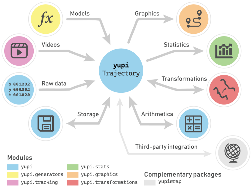
Figure 1: Visual representation of the internal structure of yupi. Each possible path in the graph represents a possible application of yupi. Node colors resemble the internal yupi module containing the specific tool, with exception of gray, that represents the complementary software package yupiwrap, designed to ease the conversion process among yupi and third-party software.

2.1 Core module

Empirically, a trajectory is the path that a body describes through space. More formally, it is a function $\mathbf{r}(t)$, where $\mathbf{r}$ denotes position and $t$, time. Here, $\mathbf{r}$ extends from the origin of an arbitrary reference frame, to the moving body. Consequently, the core module contains the class Trajectory to represent a moving object described by some position vector, $\mathbf{r}(t)$, of an arbitrary number of dimensions.

Since time is a continuous, machines have to deal with a discretized (i.e., sampled) version of the trajectory, $\mathbf{r}(t)$. As soon as one considers a sampled trajectory, it always requires an associated time vector, $\mathbf{t}=(t_{1},...,t_{n})^{\intercal}$, where each $t_{i}$ represents the timestamp of the $i$-th sample and $n$ is the total number of samples. For brevity, the sampled trajectory is often referred to as trajectory as well, so we may use either term. For instance, in the typical 3-dimensional case, a trajectory can be defined by the vector $\mathbf{r}_{i}=(x_{i},y_{i},z_{i})^{\intercal}$, where each component denotes a spatial coordinate.

The core module defines the way to retrieve specific quantities from a trajectory such as position components or velocity time series. It also defines operations among trajectories such as addition, scaling or rotation. In addition, storage functionalities are provided for different importing/exporting formats. Resources from this module can be imported directly from yupi and will be summarized next.

2.1.1 Vector objects

It is very common to refer to position or velocity as a vector that changes through time. According to this, a Vector class was created to store all the time-evolving data in a trajectory. Iterating over each sample of these Vector time series one can get the vector components at specific time instants.

This class was implemented by wrapping the numpy ndarray type. The main reason that motivated this choice, along with all the benefits from the ndarray class itself, was to gain verbosity over the usual operations on a vector. For instance, getting a specific component of a vector, the differences between its elements, or even calculating its norm, can be done with a vector instance by accessing properties such as: norm or delta. In addition, properties x, y, z allow acquiring data from one specific axis in multidimensional vectors.

Although users may not directly instantiate Vector objects, these are used all along the library to represent every time-evolving data one could get from a trajectory such as position, velocity, acceleration and time itself.

2.1.2 Trajectory objects

A Trajectory object is yupi’s essential structure. Its time evolving data, stored as Vector objects, can be accessed through the attributes t, r, v and a, standing for time, position, velocity and acceleration, respectively.

Trajectory data is typically stored in different manners, e.g., a single sequence of $d$-dimensional points where each point represents the position at a time instant or, alternatively, $d$ sequences of position components. Regardless of the input manner, yupi offers the way to create Trajectory objects from raw data.

By default, trajectories will be assumed to be uniformly spaced every 1 unit of time. However, custom time information can also be supplied. Then, position and time are used to automatically estimate velocity and acceleration according to one of the supported numerical methods: linear finite differences and the method proposed by (Fornberg, 1988).

Trajectory objects can be shifted or scaled by performing arithmetic operations on either all position components of a subset of them. For the specific case of 2- or 3-dimensional trajectories, rotation methods were conveniently implemented to ease visualization tasks, named rotate_2d and rotate_3d.

Furthermore, operations among trajectories are also defined. Trajectories with the same dimension and time vector can be added, subtracted or multiplied together. These operations are defined point-wise and can be used via the conventional operators for addition, subtraction and multiplication: +, - and *.

2.2 Generators module

The usage of randomly generated data is common in different research approaches related to trajectory analysis (Tuckerman, 2010). In this section we tackle three classical models that usually explain (or serve as a framework to explain) a wide number of phenomena connected to Biology, Engineering and Physics: Random Walks (Pearson, 1905), the Langevin model (Langevin, 1908) and Diffusing-Diffusivity model (Chechkin et al., 2017).

In yupi, the aforementioned models are implemented by inheritance of an abstract Generator class. Any Generator object must be used specifying four parameters that characterize numerical properties of the generated trajectories: T (total time), dim (trajectories dimension), N (number of trajectories to be generated) and dt (time step). Additionally, a seed parameter can be specified to initialize a random number generator (rng) which is used locally to reproduce the same results without changing the global seed.

Next, we will briefly describe the foundations of each model implemented in yupi and explain how to use them to generate ensembles of trajectories like the ones sketched in Figure 2a.

2.2.1 Random walk

A Random Walk is a random process that, in a $d$-dimensional space ($d\!\in\!\mathbb{N}^{+}$), describes a path consisting in a succession of independent random displacements. Since the extension to more than one dimension is straightforward, we shall formulate the process in its simplest way:

Let $Z_{1},...,Z_{i},...,Z_{n}$ be independent and identically distributed random variables (r.v.’s) with $P(Z_{i}=-1)=q$, $P(Z_{i}=0)=w$ and $P(Z_{i}=1)=p$, and let also $X_{i}=\sum_{j=1}^{i}Z_{j}$. Interpreting $Z_{i}$ as the displacement at the $i$-th time instant, the collection of random positions $\{X_{i},1\leq i\leq n\}$ defines the well known random walk in one dimension.

It is possible to extend this definition by allowing the walker to perform displacements of unequal lengths. Hence, if we denote by $L_{i}$ the variable that accounts for the length of the step at the $i$-th time instant, the position will be given by:

$$X_{i}=\sum_{j=1}^{i}L_{j}Z_{j},\qquad i=1,2,...,n$$ (1)

A process governed by Equation 1 in each axis is a $d$-dimensional Random Walk. Note that our definition is slightly more general than the classical, i.e., it allows the walker to remain at rest in a node of a network that is not necessarily evenly spaced. These generalized versions are often known as Lazy Random Walks (Lawler and Limic, 2010) or Random Walks with multiple step lengths (Boczkowski et al., 2018).

We define a trajectory by having a position vector whose components are described by Equation 1. For instance, in the 3-dimensional case, $\mathbf{r}_{i}=(X_{i}^{(1)},X_{i}^{(2)},X_{i}^{(3)})$.

In yupi, this model is accessible through the RandomWalkGenerator class. To use it, the probabilities $q$, $w$ and $p$ need to be defined for each dimension:

    prob = [[.5, .1, .4],   # x-axis
            [.5,  0, .5]]   # y-axis

Then, trajectories are generated as:

from yupi.generators import RandomWalkGenerator
rw = RandomWalkGenerator(T, dim, N, dt, prob)
trajs = rw.generate()

In this case, the variable trajs contains a list of N generated Trajectory objects. Note that the first 4 parameters passed to the RandomWalkGenerator are required by any kind of generator in yupi as explained in the beginning of this section.

2.2.2 Langevin model

An Ornstein-Uhlenbeck process (Uhlenbeck and Ornstein, 1930), well known by its multiple applications to describe processes from different fields (Lax et al., 2006), is defined in the absence of drift by the linear stochastic differential equation:

$$dv=-\gamma\,v\,dt+\sigma\,dW$$ (2)

where $\gamma$ and $\sigma$ are positive constants and $W$ is a Wiener process. Equation 2 is also written as a Langevin equation (Langevin, 1908), which in the multi-dimensional case takes the form:

$$\frac{d}{dt}\mathbf{v}(t)=-\gamma\mathbf{v}(t)+\sigma\boldsymbol{\xi}(t)$$ (3)

where $\boldsymbol{\xi}(t)$ is a white noise; $\sigma$, the scale noise parameter; and $\gamma^{-1}$, a characteristic relaxation time of the process.

In trajectory analysis, $\mathbf{v}(t)$ is intended to denote velocity, so the position vector is given by:

$$\mathbf{r}(t)=\int_{0}^{t}\mathbf{v}(t^{\prime})\,dt^{\prime}$$ (4)

Equations 3 and 4 can be solved numerically if the initial conditions $\mathbf{v}(0)=\mathbf{v}_{0}$ and $\mathbf{r}(0)=\mathbf{r}_{0}$ are known.

LangevinGenerator is the class offered by yupi to generate trajectories that follow this model. By conveniently setting the parameters described above (i.e., $\gamma$, $\sigma$, $\mathbf{v}_{0}$ and $\mathbf{r}_{0}$) several real-life scenarios can be modeled. In Section 3.2, a Langevin model is used to simulate the motion of a Lysozyme molecule in an aqueous medium.

2.2.3 Diffusing-Diffusivity model

Slow environmental relaxation has been found in soft matter for colloidal particles diffusing in an environment of biopolymer filaments and phospholipid tube assemblies (Wang et al., 2012). Non-Gaussian distribution of increments was observed even when the diffusive dynamics exhibit linear growth of the mean square displacement. A model framework of a diffusion process with fluctuating diffusivity that reproduces this interesting finding has been presented as Diffusing Diffusivity Model. Namely:

$$\frac{d}{dt}\mathbf{r}(t) =\sqrt{2D(t)}\,\boldsymbol{\xi}(t)$$ (5a)

$$D(t) =\mathbf{Y}^{2}(t)$$ (5b)

$$\frac{d}{dt}\mathbf{Y}(t) =-\frac{1}{\tau}\mathbf{Y}(t)+\sigma\boldsymbol{\eta}(t)$$ (5c)

where $\boldsymbol{\xi}(t)$ and $\boldsymbol{\eta}(t)$ are Gaussian white noises and $D(t)$, the diffusion coefficient, is a random function of time expressed as the square of the auxiliary variable, $\mathbf{Y}(t)$.

In other words, the coupled set of stochastic differential equations (5) predicts a Brownian but Non-Gaussian diffusion, where the position, $\mathbf{r}(t)$, is described by an over-damped Langevin equation with the diffusion coefficient being the square of an Ornstein-Uhlenbeck process. The model has been discussed and solved analytically by (Chechkin et al., 2017; Thapa et al., 2018).

The class devoted to generate trajectories modeled by the Equations 5 is called DiffDiffGenerator. Implementation details can be found in the software documentation.

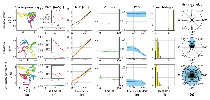
Figure 2: Statistical analysis of three generated ensembles of N=1000 two-dimensional trajectories. Rows listed from top to bottom correspond to an ensemble generated using a Random Walk, Langevin and Diffusing Diffusivity models, respectively. (a) Spacial projection of five trajectories. (b) Estimated Velocity autocorrelation function and (c) Mean Squared Displacement as a function of the lag time. (d) Kurtosis as a function of time. (e) Power Spectral Density. (f) Speed histograms. (g) Turning angle probability densities.

2.3 Stats module

The library provides common techniques based on the mathematical methods that researchers frequently use when analyzing trajectories. This section presents an overview on how to compute observables to describe them. Velocity autocorrelation function, kurtosis or mean square displacement are some typical examples.

Most of these observables were originally defined using ensemble averages (i.e., expected values at a given time instant). However, under the assumption of ergodicity, it is possible to compute the observables using time averages (i.e., by averaging the quantities among time intervals instead). In yupi the observables can be computed using both approaches. In the following subsections, we will denote by $E[\cdot]$ (i.e., expected value) the ensemble average and $\langle\cdot\rangle$ the time average.

2.3.1 Velocity autocorrelation function

The velocity autocorrelation function (VACF) is defined as the ensemble average of the product of velocity vectors at any two instants of time. Under stationary conditions, the definition is typically relaxed to the one of Equation 6a, in which one of the vectors is the initial velocity. On the other hand, Equation 6b presents the way VACF is computed by averaging over time under the assumption that both averages are equivalent (i.e., ergodic assumption).

$$C_{v}(t) =E[\mathbf{v}(0)\cdot\mathbf{v}(t)]$$ (6a)

$$\begin{split}C_{v}(\tau)&=\langle\mathbf{v}(t)\cdot\mathbf{v}(t+\tau)\rangle\\ &=\frac{1}{T-\tau}\int_{0}^{T-\tau}\mathbf{v}(t)\cdot\mathbf{v}(t+\tau)dt\end{split}$$ (6b)

Here, $\tau$ is the lag time, a time window swept along the velocity samples and $T$ is the elapsed time, where $\tau\ll T$.

It should be noted that in Equation 6b VACF is defined to be computed on a single trajectory, unlike Equation 6a that requires an ensemble. This also applies to further statistical observables that can be computed using both kinds of averaging procedures.

VACF quantifies the way in which the memory in the velocity decays as a function of time (Balakrishnan, 2008). Moreover, it can be successfully used to analyze the nature of an anomalous diffusion process (Metzler et al., 2014).

From top to bottom, Figure 2b shows VACF plots for Random Walk, Langevin and Diffusing Diffusivity generated ensembles. VACF scatter as an almost flat curve around zero for the top and bottom case, which indicates the memoryless nature of Random Walk and Diffusing Diffusivity processes. On the other hand, the center row shows an exponential decay, meaning that a Langevin model predicts some characteristic time that dominates the relaxation to equilibrium.

With yupi, one can estimate the VACF of a collection of trajectories (e.g., the ensemble generated in Section 2.2.1) as:

    from yupi.stats import vacf
    trajs_vacf, trajs_vacf_std = vacf(
        trajs, time_avg=True, lag=25)

where vacf is the name of the function that computes the autocorrelation, the parameter trajs represents the array of trajectories and time_avg indicates the method to compute the observable, i.e., averaging over time with a lag time defined by lag.

The computation of the remaining observables can be coded in a similar way. Next, for the sake of brevity, we will address only its theoretical foundations. In the software documentation, more examples can be found that make use of all the observables.

2.3.2 Mean square displacement

The mean square displacement (MSD) is defined in Equation 7a by an ensemble average of square displacements. In addition, the time-averaged mean square displacement (TAMSD) is computed by a moving average of the squared increments along a single trajectory. This is performed by integrating over trajectory points separated by a lag time $\tau$ that is much smaller than the overall measurement time $T$ (Equation 7b).

$$\delta^{2}(t) =E[{(\mathbf{r}(t)-\mathbf{r}(0))}^{2}]$$ (7a)

$$\begin{split}\delta^{2}(\tau)&=\langle{(\mathbf{r}(t+\tau)-\mathbf{r}(t))}^{2}\rangle\\ &=\frac{1}{T-\tau}\int_{0}^{T-\tau}{(\mathbf{r}(t+\tau)-\mathbf{r}(t))}^{2}dt\end{split}$$ (7b)

The MSD of a normal diffusive trajectory arises as a linear function of time. Therefore, it is a typical indicator to classify processes far from normal diffusion. Moreover, MSD reveals what are the time scales that characterize different diffusive regimes.

In Figure 2c a comparison of MSD plots is made for the three ensembles previously presented. Regardless of the model used, the same long time behavior can be perceived, i.e., the same scaling law arises for sufficiently long time scales. This can be seen while contrasting the MSD curves with the dashed line of slope equal to one, meaning that normal diffusion is achieved.

2.3.3 Kurtosis

Another useful statistical observable is the kurtosis. Different formulations for kurtosis have been proposed in the literature (Cain et al., 2017). The common choice for the one-dimensional case is presented as the ensemble average of Equation 8a, where $\mu$ stands for the mean velocity and $\sigma$ the standard deviation. In addition, for the multivariate case we use Mardia’s measure (Mardia, 1970) as in Equation 8b. The vector $\boldsymbol{\mu}$ is the $d$-dimensional mean velocity ($d>1$) and $\mathbf{\Sigma}$ the covariance matrix. In both cases we have omitted the explicit dependence with time, but it should be noted that the expected value is taken at a given instant.

$$\kappa(t) =E\left[\left(\frac{v-\mu}{\sigma}\right)^{4}\right]$$ (8a)

$$\kappa(t) =E[\{(\mathbf{v}-\boldsymbol{\mu})^{\intercal}\mathbf{\Sigma}^{-1}(\mathbf{v}-\boldsymbol{\mu})\}^{2}]$$ (8b)

The kurtosis measures the disparity of spatial scales of a dispersal process (Méndez et al., 2016) and it is also an intuitive means to understand normality (Cain et al., 2017).

Figure 2d shows how kurtosis converges to a value close to $8$ regardless of the model used. This is a consequence of convergence to a Gaussian density and the fact that all three processes are two-dimensional. Moreover, just in the case of the Diffusing Diffusivity model a leptokurtic regime is observed, i.e., a regime in which $\kappa\gtrsim 8$. This means that some flat-tailed density (compared with the Gaussian) aroused first and $\kappa(t)$ provides a direct way to extract, apart from the crossover time, the correlation time of the diffusion coefficient.

2.3.4 Power spectral density

The Power Spectral Density, or Power Spectrum, (PSD) of a continuous-time random process can be defined by virtue of the Wiener${-}$Khintchin theorem as the Fourier transform $S(\omega)$ of its autocorrelation function $C(t)$:

$$S(\omega)=\int_{-\infty}^{\infty}C(t)e^{-i\omega t}dt$$ (9)

Power spectrum analysis indicates the frequency content of the process. The inspection of the PSD from a collection of trajectories enables the characterization of the motion in terms of the frequency components.

For instance, when analysing the ensembles represented in Figure 2a, we notice important differences in their spectrum (see Figure 2e). In the Langevin and Diffusing Diffusivity cases the PSD shows a decay for larger frequencies as opposite to the Random Walk model, in which all frequencies contribute equally, i.e., the spectrum is distributed uniformly.

2.3.5 Histograms

Certain probability density functions can also be estimated from input trajectories (e.g., velocity and turning angle distributions).

Speed probabilty density function is a useful observable to inspect jump length statistics. For instance, Figure 2f reveals the discrete nature of the Random Walk and the rapidly decay of the tails for the Langevin and Diffusing Diffusivity plots, which is a typical indicator to discard anomalous diffusion models as candidate theories.

Figure 2f shows turning angle distributions in polar axes. For the Random Walk model just few discrete orientations are available in contrast with the other two cases: a bell-shape around zero and a uniform distribution for the Langevin and Diffusing Diffusivity model, respectively.

2.3.6 Other functionalities

In addition to the computation of statistical estimators, the stats module of yupi includes the collect function for querying specific data from a set of trajectories. If one desires to obtain only position, velocity or speed data from specific time instants, this function automatically iterates over the ensemble and returns the requested data. Moreover, collect also gets samples for a given time scale using sliding windows.

A more extensive showcase of this module can be seen in the examples provides as part of the Software Documentation.

2.3.7 Graphics module

A set of pre-configured visualization functions are included as part of yupi. Spatial projections can be visualized for the cases of 2- and 3-dimensional trajectories using plot_2d and plot_3d functions. For instance, each subplot in Figure 2a is the outcome of plot_2d for different ensembles.

In addition, specific plots were added to ease the visualization of the observables offered by the module yupi.stats). This customized plotting functions were designed to highlight statistical patterns following the commonly used standards in the literature (e.g., by default, plots of angle distributions are displayed in polar coordinates and the y- and x-axis of the Power Spectral Density plots in logarithmic scale). All the plots in Figure 2b-g were produced using the aforementioned functions.

All these functions were conceived to allow plots customization through case-specific parameters (e.g., PSD can be plotted as a function of the frequency or angular frequency). Moreover, since all the predefined plots were implemented over matplotlib, the users can fully customize their plots via keyword arguments (kwargs parameter) that will override any default values imposed by the specific yupi plotting function.

2.4 Transformation module

The yupi.transformations module can be used when the desired outcome is a “transformed” version of a given trajectory that does not modify the trajectory itself. Since several methods of this kind can be applied from standard signal processing libraries (e.g., scipy.signal) we kept this module simple. Therefore, we included mostly specific resources that were both useful in the context of trajectory analysis and uncommon in most popular signal processing libraries.

2.4.1 Trajectory filters

The module scipy.signal offers methods to convolve, to spline or to apply low-, band- and high-pass filters. However, we have included a convenient filter especially useful in the context of animal behavior, where the instant velocity vector is sometimes approximated to a local weighted average over past values (Li et al., 2011). This is presented as the convolution:

$$\mathbf{v}_{s}(t)=\Omega\int_{0}^{t}e^{-\Omega(t-t^{\prime})}\mathbf{v}(t^{\prime})dt^{\prime}$$ (10)

where $\Omega$ is a parameter that accounts for the inverse of the time window over which the average is more significant. A filter defined by Equation 10 preserves directional persistence and produces a smoothed version of a trajectory whose velocity as a function of time is given by $\mathbf{v}_{s}(t)$. Therefore, position can be recovered with the help of Equation 4.

This “exponential-convolutional” filter can be used as:

from yupi.transformations import (
    exp_convolutional_filter)
smooth_traj = exp_convolutional_filter(
    traj, ommega=5)

Future releases of the library may include new filters required for specific applications in trajectory analysis.

2.4.2 Trajectory re-samplers

There are several applications that require trajectories to be sampled in specific time arrays. The most obvious case is when a trajectory has a non-uniform time array and it is desired to produce an equivalent trajectory sampled periodically on time. This can be achieved using the resample function:

    from yupi.transformations import resample
    t1 = resample(traj, new_dt=0.3, order=2)

Notice that, by default, the library uses a linear interpolation to resample the trajectory. However, the order of the estimation can be controlled using the order parameter.

Equivalently, a new trajectory can be obtained for a given time array that is not required to be uniformly sampled by specifying the time array itself as the $new\_t$ parameter instead of $new\_dt$ while calling the resample function.

We also included a simple sub-sampling method designed for uniformly-sampled trajectories. It produces trajectories that keep only a fraction of the original trajectory points. It can be used as:

    from yupi.transformations import subsample
    compact_traj = subsample(traj, step=5)

where the step parameter is specifying how many sample points will be skipped.

2.5 Tracking module

The tracking module contains all the tools related to retrieving trajectories from video inputs. Although yupi works with trajectories of an arbitrary number of dimensions, the scope of this module is limited to two-dimensional trajectories due to the nature of video sources. However, inspired by several practical scenarios in which tracking techniques are required to extract meaningful information, we decided to include these tools as part of the library.

We will refer to tracking as the process of retrieving the spatial coordinates of moving objects in a sequence of images. Notice that this is not always possible for any image sequence. Some requirements should be met in order to extract meaningful information.

Along this section, we will assume that any video used for tracking purposes was taken keeping a constant distance from the camera to the plane in which the target objects are moving.

2.5.1 Tracking of objects of interest

When following a given object in a video, the aim of tracking techniques is to provide its position vector with respect to the camera, which we will denote by $\mathbf{r}_{i}^{\mathrm{(oc)}}$ (superscript $(oc)$ stands for object-to-camera reference and subscript $i$ stands for the $i$-th frame the vector is referred to).

If the dimensions of the object being tracked are small enough (i.e., comparatively smaller than the distance covered in the whole trajectory) the centroid of the object determines the only degrees of freedom of the movement since orientation can be neglected. This point is frequently taken as the position of the object.

To determine the actual position of an object on every frame, a tracking algorithm to segment the pixels belonging to the object from the background is required. Five algorithms are implemented in yupi: ColorMatching, FrameDifferencing, BackgroundSubtraction, TemplateMatching and OpticalFlow. A detailed explanation of the basics of the aforementioned algorithms can by found in Frayle-Pérez et al. (2017). All those algorithms attempt to solve the same problem using very different strategies. Therefore, it happens often that under specific conditions one of them may outperform the others.

To speed up the tracking process, yupi uses a region of interest (ROI) around the last known position of the tracked objects. Then, on every frame, the algorithm searches only inside this region instead of in the whole image. When it founds the new position, it updates the center of the region of interest for the next frame. When the tracking ends, the time evolution of the central position of the ROI is used to reconstruct the trajectory of the tracked object.

The library enables the extraction of Trajectory objects from videos through ObjectTracker instances which are defined by a tracking algorithm and a ROI. For a given video, several objects can be tracked concurrently using an independent ObjectTracker for each one of them. Finally, a TrackingScenario is the structure that groups all trackers and iterates through the video frames while resolving the desired trajectories for each tracker.

2.5.2 Tracking a camera in motion

Sometimes the camera used to track the object under study is also in motion and it is able to translate and to execute rotations around a vertical axis. Therefore, knowledge regarding positions and orientations of the camera during the whole experiment is required to enable a correct reconstruction of the trajectory relative to a fixed coordinate system. One way to tackle this issue is inferring the movement of the camera by means of the displacements of the background in the image. Preserving the assumption that the camera only moves in a plane parallel to the plane in which the objects are moving, the motion of the camera can be estimated by tracking a number of background points between two different frames and solve the optimization problem of finding the affine matrix that best transforms the set of points. This means that for a rotation angle $\theta$, a scale parameter $s$, and displacements $t_{x}$ and $t_{y}$, an arbitrary vector $(x,y)$ will become

$$\begin{bmatrix}x^{\prime}\\ y^{\prime}\\ 1\end{bmatrix}=\begin{bmatrix}s\cos\theta&-\sin\theta&t_{x}\\ \sin\theta&s\cos\theta&t_{y}\\ 0&0&1\end{bmatrix}\begin{bmatrix}x\\ y\\ 1\end{bmatrix}$$ (11)

Therefore, the problem reduces to find the vector $(\theta,t_{x},t_{y},s)$ that minimizes the least square error of the transformation. Under the assumption that the camera is always at approximately the same distance from the background, the scale parameter should be close to 1. As long as the mean square error remains under a given threshold and the condition $s\approx 1$ holds, the validity of the estimation is guaranteed. Hence, the collection $\{\theta_{i},t_{xi},t_{yi}\}$, where $i$ stands for the frame number, contains all the information necessary to compute the positions and orientations of the camera.

2.5.3 Tracking objects and camera simultaneously

As was mentioned above, the position of the object under study with respect to the camera in the $i$-th frame has been denoted by $\mathbf{r}_{i}^{\mathrm{(oc)}}$. If the camera also moves and we can follow features on the background from one frame to the another, we are able to calculate the parameters $(\theta_{i},t_{xi},t_{yi})$ of the affine matrix that transforms the $(i{-}1)$-th into the $i$-th frame.

The question we now face is: How to compute the position $\mathbf{r}_{i}\equiv\mathbf{r}_{i}^{\mathrm{(ol)}}$ of the object with respect to the frame of reference fixed to the lab in the $i$-th frame?

Let us label as $\alpha_{i}$ the cumulative angular differences of the affine matrix parameter $\theta$ until the $i$-th frame (Equation 12a) and $\mathbf{t}_{i}=(t_{xi},t_{yi})^{\intercal}$ the vector of displacements of the affine transformation. Let $\mathbf{R}$ be the rotation matrix (i.e., the upper-left $2{\times}2$ block of the matrix in Equation 11 when $s=1$). Then, the position of the camera in the lab coordinate system, $\mathbf{r}_{i}^{(\mathrm{cl})}$, can be determined in an iterative manner as follows:

$$\alpha_{i} =\sum_{j=1}^{i}\theta_{j}\qquad$$ (12a)

$$\mathbf{r}_{i}^{\mathrm{(cl)}} =\mathbf{R}^{-1}(\alpha_{i})\cdot(-\mathbf{t}_{i})+\mathbf{r}_{i-1}^{\mathrm{(cl)}}$$ (12b)

$$\mathbf{r}_{i} =\mathbf{R}^{-1}(\alpha_{i})\cdot\mathbf{r}_{i}^{\mathrm{(oc)}}+\mathbf{r}_{i}^{\mathrm{(cl)}}$$ (12c)

Therefore, the desired position of the object under study, $\mathbf{r}_{i}$, can be computed by Equation 12c in terms of its position in the frame of reference fixed to the camera, $\mathbf{r}_{i}^{\mathrm{(oc)}}$, the absolute position of the camera, $\mathbf{r}_{i}^{\mathrm{(cl)}}$, and the camera orientation, $\alpha_{i}$.

This whole process is simplified in yupi by the CameraTracker class. By default, yupi assumes that the position of the camera remains fixed. However, in order to estimate the motion of a camera and use it to retrieve the correct position of the tracked objects, the user only needs to create a CameraTracker object and pass it to the TrackingScenario.

2.5.4 Removing distortion

When recording video, the output images generally contain some distortion caused by the camera optics. This is important when spatial measurements are being done using videos or photographs. To correct these errors some adjustments must be applied to each frame. Applying an undistorter function to the videos is possible in yupi using the ClassicUndistorter or the RemapUndistorted.

2.6 Integration with other software packages

Along with yupi, we offer a Python library called yupiwrap (available in https://github.com/yupidevs/yupiwrap), designed to ease the integration of yupi with other libraries for handling trajectories. Two-way conversions between a given yupi Trajectory and the data structure used by the third-party library can be made via yupiwrap. This approach enables users to seamlessly use the resources needed from either library.

2.6.1 Integration with traja

Traja Python package is a toolkit for numerical characterization and analysis of moving animal trajectories (Shenk et al., 2021). It provides some machine learning tools that aren’t yet available in yupi.

To convert from yupi to traja let us first consider an arbitrary yupi Trajectory:

    traj = Trajectory(
        x=[0, 1.0, 0.63, -0.37],
        y=[0, 0, 0.98, 1.24])

and then the conversion to a traja DataFrame is done by:

    from yupiwrap import yupi2traja
    traj_traja = yupi2traja(traj)

Notice that only two-dimensional trajectories can be converted to a traja object due to its own limitations. The conversion in the opposite direction can be done in a similar way by using traja2yupi instead.

2.6.2 Integration with tracktable

Tracktable provides a set of tools for handling two- and 3-dimensional trajectories even in geospatial coordinate systems (Sandialabs, 2021). The core data structures and algorithms in this package are implemented in C++ for speeding up computation and more efficient memory usage.

If we consider the same yupi Trajectory from the previous example, we can convert it into a Tracktable object using:

    from yupiwrap import yupi2tracktable
    traj_track = yupi2tracktable(traj)

In this case, all trajectories with a number of dimensions within 1 to 3 can be converted into Tracktable objects. The conversion in the opposite direction can also be done by importing tracktable2yupi.

3 Examples

In this section, we illustrate the usage of yupi through different examples that require a complex integration of different modules. The examples were chosen to showcase the potential of the library to solve problems that heavily rely on trajectory analysis and its extraction from video sources. Most of the examples reproduce core results from published research. Others include original approaches to verify known properties of different phenomena. All in all, the collection of examples is designed to provide a quick starting point for new research projects involving trajectory data, with a particular focus in environmental modelling.

For simplicity, we omit some technical details related to its implementation. However, we provide a detailed version of these examples in the software documentation with required multimedia resources and source code, available in a repository conceived for yupi examples.

3.1 Identifying environmental properties through tracking and trajectory processing

Visual tracking has proven to be an effective method for the study of physical and biological processes. Moreover, indirect measurements from the enviroment can also be retrieved from the analysis of the directly measured trajectories. For instance, tracking techniques have empowered researchs on animal behavior, which can improve the effectiveness and success of conservation management programs (Greggor et al., 2019) and gives valuable information about ecosystem changes (Rahman and Candolin, 2022). More especifically, in (Yuan et al., 2018) the authors infered the water quality through the analysis of features from fish trajectories. Furthermore, the work of (Panwar et al., 2020) shows how to automate the detection of waste in water bodies using images from the environment. In addition, the measurements of river flows have also benefited from the tracking of key features using satellital images (Gleason et al., 2017).

In the work of (Stephenson et al., 1999), it was shown how the stresses of turning wheels in the grounds can affect vegetation cover, plant health and diversity, as well as reducing underground rhizomes (roots) generation. Inspired on these facts, we decided to reproduce the tracking results from the work of (Amigó-Vega et al., 2019) on the study of the motion of vehicles on granular materials. They reported the analysis of the trajectories performed by a scaled-size wheel while rolling on sand at two different gravitational accelerations, exploiting a frugal instrument design (Viera-López et al., 2017; Altshuler et al., 2014). Figure 3a shows a sketch of the instrument where a camera on top captures the motion of the wheel while rolling around a pivot. This example was built using one of the original videos provided by the authors (see Figure 3b).

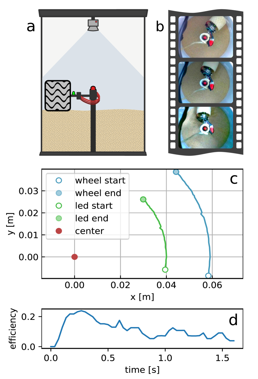
Figure 3: Efficiency of the rolling process computed for a wheel moving across granular material at a constant angular velocity $\omega=4$ rad/s under a gravitational acceleration as the one on Mars. (a) Experimental setup composed by the wheel electro-mechanical system to ensure the constant angular velocity and a camera to record its motion. (b) Sample frames from a video where the wheel moves around the pivot. (c) Estimated positions of the wheel and the LED used as a reference to track it. (d) Estimation of the rolling efficiency for a single realization of the experiment, showing a strong consistence with the ones reported in the original paper (Amigó-Vega et al., 2019).

In the video, one observes the wheel forced to move on sand at a fixed angular velocity. In optimal rolling conditions, one can expect it to move at a constant linear velocity. However, due to slippage and compaction-decompaction of the granular soil, the actual linear velocity differs from the one expected under ideal conditions. To study the factors that affect the wheel motion, the first step is quantifying how different the rolling process is with respect to the expected one in ideal conditions. This example focuses on the problem of capturing the trajectory of the wheel and computing the efficiency of the rolling process.

We start by creating two trackers: one for the central pivot and one for the green led attached next to the wheel. Since the central pivot should not move significantly, we can track it using TemplateMatching algorithm, by comparing every frame with a template of the object. As the led colors differs from the rest of the image, we can use ColorMatching algorithm to track its position.

Both trackers are used among the TrackingScenario to retrieve the trajectories of both objects along the video. It is worth to mention that, for an accurate estimation, it is required to know the scale factor (i.e., the number of pixels required to represent 1 m).

By calling the track method, the tracking process should produce two trajectories (one for each tracker). Notice that these trajectories (i.e., ${t_{\text{led}}}$ and ${t_{\text{pivot}}}$) are referred to a frame of reference placed on the bottom left corner of the image as shown in Figure 3.

Then, using the arithmetic operations from yupi it is possible to estimate the trajectory of the LED referred to the center pivot by simply subtracting them as: $t_{\text{led\_centered}}=t_{\text{led}}-t_{\text{pivot}}$.

Since the LED and the center of the wheel are placed at a constant distance of 0.039 m, we can estimate the trajectory of the wheel referred to the center pivot:

    wheel_centered = led_centered.copy()
    wheel_centered.add_polar_offset(0.039, 0)

Finally, the trajectory of the wheel referred to its initial position, can be obtained by subtracting the initial from the final position after completing the whole trajectory.

wheel = wheel_centered - wheel_centered.r[0]

Now, assuming no slippage, we can compute the linear velocity as: $v_{\text{max}}=\mathbf{\omega}R$ = $(4\,\mathrm{rad/s})\times(0.07\,\mathrm{m})$ and measure the actual linear velocity using the trajectory estimated by the tracking process:

    v_actual = wheel.v.norm

By dividing $v_{\text{actual}}$ by $v_{\text{max}}$, we can estimate the efficiency of the rolling as described in (Amigó-Vega et al., 2019). The temporal evolution of the efficiency for the single experiment can be observed in Figure 3d.

We can notice how the linear velocity of the wheel is not constant despite the constant angular velocity, due to slippage in the terrain. Even when we are observing only one realization of the experiment, and assuming the angular velocity of the wheel being perfectly constant, we notice the consistency of this result with the one reported in the original paper.

Despite the specific nature of this example, it is easy to make a straightforward extension of its usage across many other problems that may require the identification of objects from video sources and the application of arithmetic operations over trajectories to indirectly measure any derived quantities. In that regard, we included in the software documentation additional examples related to trajectory tracking that partially reproduce key results from published research: The work of (Díaz-Melián et al., 2020) where the authors study the penetration of objects into granular beds; The work of (Frayle-Pérez et al., 2017), where the authors studied the capabilities of different image processing algorithms that can be used for tracking of the motion of insects under controlled environments and the work of (Serrano-Muñoz et al., 2019) that extends on the previous one by proposing the design of a robot able to track millimetric-size walkers in much larger distances by tracking both insect and camera simultaneusly.

3.2 Equation-based simulations: A molecule immerse in a fluid

Several systems can be explained using stochastic models as the ones shown in Section 2.2. To accurately describe them, it is required to adjust the parameters of the model according to measureable data. Next, we will illustrate how to use yupi to generate simulated trajectories of a lysozyme in water using the Langevin model presented in Section 2.2.2. We corroborate that the model correctly predicts the order of magnitude of molecule’ speed values.

Proteins contribute greatly in environmental processes and are fundamental in soil and ecosystem health (Li et al., 2020). Since interactions of proteins with charged surfaces are important in many applications such as biocompatible medical implants (Subrahmanyam et al., 2002), the dynamics of lysozyme and its hydration water has been characterized under electric field effects in different water environments (Favi et al., 2014). Alongside, the thermal velocity for a sizeable particle immerse in water such as a lysozyme molecule at room temperature has been estimated to be around $10\,\mathrm{m/s}$ (Berg, 2018).

The right hand side of the Langevin equation (3) can be interpreted as the net force acting on a particle. This force can be written as a sum of a viscous force proportional to the particle’s velocity (i.e., Stokes’ law with drag parameter, $\gamma=1/\tau$, with $\tau$ a correlation time), and a noise term, $\sigma\,\boldsymbol{\xi}(t)$, representing the effect of collisions with the molecules of the fluid. Therefore, (3) can be written in a slightly different way by noting that there is a relation between the strength of the fluctuating force, $\sigma$, and the magnitude, $1/\tau$, of the friction or dissipation, which is known as the Fluctuation-dissipation theorem (Kubo, 1966; Srokowski, 2001). Consequently, in terms of experimental measured quantities and in differential form, the Langevin equation can be reformulated in the light of stochastic processes by

$$d\mathbf{v} =-\frac{1}{\tau}\mathbf{v}dt+\sqrt{\frac{2}{\tau}\left(\frac{kT}{m}\right)}\,d\mathbf{W}$$ (13a)

$$\frac{1}{\tau} =\gamma=\frac{\alpha}{m}=\frac{6\pi\eta a}{m}$$ (13b)

where $k$ is the Boltzmann constant, $T$ the absolute temperature, and $m$ the mass of the particle. Equation 13b provides an operational method to measure the correlation time in terms of the Stoke’s coefficient, $\alpha$, which depends on the radius of the particle, $a$, and the fluid viscosity, $\eta$.

Lysozyme enzymes are molecules with a high molecular weight ($\sim 10^{4}\,\mathrm{g/mol}$) (Colvin, 1952). So, it is reasonable to expect a brownian behavior in the limit of large time scales when the particle is subjected to the molecular collisions of the surrounding medium (e.g., an aqueous medium). Then, Equation 13a is a good choice to use as a model.

By setting the total simulation time T, the dimension dim, the number N and the time step dt of the simulated trajectories, as well as the coefficients gamma and sigma of Equation 3, we can instantiate the LangevinGenerator class and generate an ensemble of trajectories:

from yupi.generators import LangevinGenerator
lg = LangevinGenerator(
    T, dim, N, dt, gamma, sigma)
trajs = lg.generate()

Figure 4 shows the velocity probability density function that the model predicts. Apart from the typical Gaussian shape that arises when massive particles are jiggling, the standard deviation (vertical red lines) is in agreement with the previous estimation for the local thermal velocity.

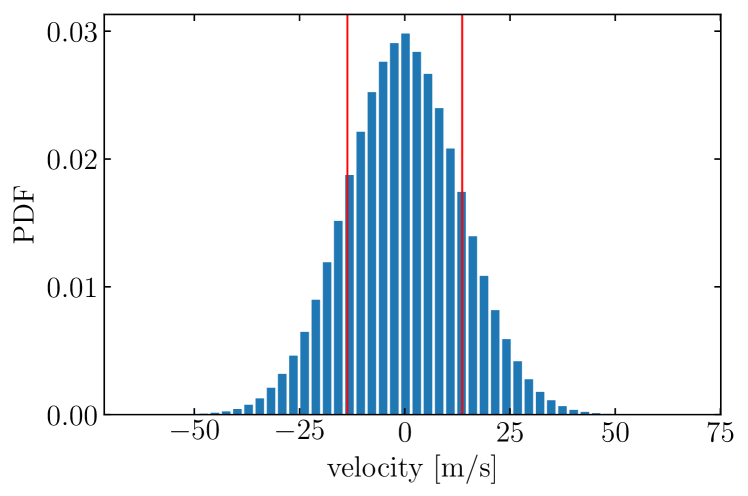
Figure 4: Gaussian velocity distribution predicted by Equation 13a for trajectories of a lysozyme molecule in water. Standard deviation, depicted as vertical red lines, coincides with those values in which $\langle v^{2}\rangle^{1/2}\sim 10\,\mathrm{m/s}$.

Another equation-based simulation is presented as part of the complementary examples provided in yupi documentation. It covers the computation of the probability density function for displacements at different time instants for the case of a one-dimensional process that follows the equations of a Diffusing Diffusivity model (see Section 5). The example reproduces important results from the paper presented by (Chechkin et al., 2017).

3.3 Time series analysis: water consumption examination

This example showcases the usage of yupi beyond “real” trajectories. We reproduce an example from (Hipel and McLeod, 1994) in the context of hydrological studies by simply treating a time series as an abstract trajectory.

Seasonal autoregressive integrated moving average
(SARIMA) models are useful for modelling seasonal time series in which the mean and other statistics for a given season are not stationary across the years. Some types of hydrological time series which are studied in water resources engineering could be nonstationary. For example, socio-economic factors such as an increasing of population growth in the city of London, Ontario, Canada since the Second World War to 1991, caused a greater water demand in the period (Hipel and McLeod, 1994). Figure 5a shows the average monthly water consumption (in millions of liters per day) from 1966 to 1988 for this city. The increasing trend around which the seasonal data fluctuates reveals nonstationary characteristics. As a consequence, autocorrelation analysis was used by (Hipel and McLeod, 1994) in the design and study of a SARIMA model for the water usage time series.

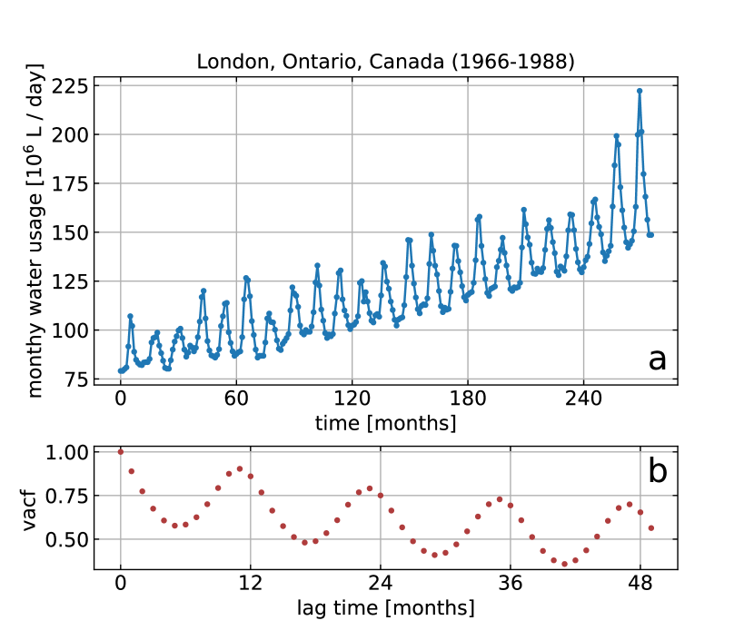
Figure 5: Analysis of water consumption in for the city of London, Ontario, Canada. (a) Seasonality of the average monthly water usage (1966-1988). The sinusoidal pattern on top of the linear trend accounts for nonstationarity. (b) Slow decreasing of the normalized autocorrelation function as a function of the lag time. Oscillations are portrayed with a period of a year. (Original plots can be found in Figures VI.2/12.4.1 pages 417/440, in (Hipel and McLeod, 1994).)

First, let waterusage be the variable in which the time series has been stored. Visualization of the data shown in Figure 5a can be done using:

from yupi import Trajectory
traj = Trajectory(x=np.cumsum(water_usage))
plt.plot(traj.v.x)

Computation and visualization of the autocorrelation function depicted in Figure 5b (see Section 2.3.1 for theoretical details) can be simply coded as:

from yupi.stats import vacf
from yupi.graphics import plot_vacf
acf, _ = vacf([traj], time_avg=True, lag=50)
plot_vacf(acf / acf[0], traj.dt, lag=50,
    x_units=’months’, y_units=None)

4 Conclusions

This contribution presents yupi, a general purpose library for handling trajectory data. Our library proposes an integration of tools from different fields conceived as a complete solution for research applications related to obtaining, processing and analyzing trajectory data. Resources are organized in modules according to their nature. However, consistency is guaranteed using standardized trajectory data structures across every module.

We have shown the effectiveness of the tool by reproducing results reported in a number of research papers. We believe the examples illustrating the simplicity of yupi should enable researchers from different fields to become more proficient in processing and analyzing trajectories even with minimal programming knowledge.

The current version of yupi does not provide specific functionalities to process geo-spacial data. Considering the wealth of available tools to tackle these specific tasks, we encourage the re-utilization of existing approaches for specific use cases by providing an extension to simplify two-way conversions of data among some existing trajectory-related software libraries.

References

- Altshuler et al. (2013) Altshuler, E., Miño, G., Pérez-Penichet, C., del Río, L., Lindner, A., Rousselet, A., Clément, E., 2013. Flow-controlled densification and anomalous dispersion of e. coli through a constriction. Soft Matter 9, 1864–1870.
- Altshuler et al. (2014) Altshuler, E., Torres, H., González-Pita, A., Sánchez-Colina, G., Pérez-Penichet, C., Waitukaitis, S., Hidalgo, R., 2014. Settling into dry granular media in different gravities. Geophysical Research Letters 41, 3032–3037.
- Amigó-Vega et al. (2019) Amigó-Vega, J., Serrano-Muñoz, A., Viera-López, G., Altshuler, E., 2019. Measuring the performance of a rover wheel in martian gravity. Revista Cubana de Física 36, 46–50.
- Balakrishnan (2008) Balakrishnan, V., 2008. Elements of nonequilibrium statistical mechanics. volume 3. Springer.
- Balogun et al. (2021) Balogun, A.L., Yekeen, S.T., Pradhan, B., Yusof, K.B.W., 2021. Oil spill trajectory modelling and environmental vulnerability mapping using gnome model and gis. Environmental Pollution 268, 115812.
- Berg (2018) Berg, H.C., 2018. Random walks in biology, in: Random Walks in Biology. Princeton University Press.
- Boczkowski et al. (2018) Boczkowski, L., Guinard, B., Korman, A., Lotker, Z., Renault, M., 2018. Random walks with multiple step lengths, in: Latin American Symposium on Theoretical Informatics, Springer. pp. 174–186.
- Cain et al. (2017) Cain, M.K., Zhang, Z., Yuan, K.H., 2017. Univariate and multivariate skewness and kurtosis for measuring nonnormality: Prevalence, influence and estimation. Behavior research methods 49, 1716–1735.
- Chechkin et al. (2017) Chechkin, A.V., Seno, F., Metzler, R., Sokolov, I.M., 2017. Brownian yet non-gaussian diffusion: from superstatistics to subordination of diffusing diffusivities. Physical Review X 7, 021002.
- Colvin (1952) Colvin, J.R., 1952. The size and shape of lysozyme. Canadian Journal of Chemistry 30, 831–834.
- De Cáceres et al. (2019) De Cáceres, M., Coll, L., Legendre, P., Allen, R.B., Wiser, S.K., Fortin, M.J., Condit, R., Hubbell, S., 2019. Trajectory analysis in community ecology. Ecological Monographs 89, e01350.
- Demšar et al. (2015) Demšar, U., Buchin, K., Cagnacci, F., Safi, K., Speckmann, B., Van de Weghe, N., Weiskopf, D., Weibel, R., 2015. Analysis and visualisation of movement: an interdisciplinary review. Movement ecology 3, 1–24.
- Díaz-Melián et al. (2020) Díaz-Melián, V., Serrano-Muñoz, A., Espinosa, M., Alonso-Llanes, L., Viera-López, G., Altshuler, E., 2020. Rolling away from the wall into granular matter. Physical Review Letters 125, 078002.
- Favi et al. (2014) Favi, P.M., Zhang, Q., O’Neill, H., Mamontov, E., Diallo, S., 2014. Dynamics of lysozyme and its hydration water under an electric field. Journal of biological physics 40, 167–178.
- Figueroa-Morales et al. (2020) Figueroa-Morales, N., Rivera, A., Soto, R., Lindner, A., Altshuler, E., Clément, E., 2020. E. coli “super-contaminates” narrow ducts fostered by broad run-time distribution. Science advances 6, eaay0155.
- Fornberg (1988) Fornberg, B., 1988. Generation of finite difference formulas on arbitrarily spaced grids. Mathematics of computation 51, 699–706.
- Frayle-Pérez et al. (2017) Frayle-Pérez, S., Serrano-Muñoz, A., Viera-López, G., Altshuler, E., 2017. Chasing insects: a survey of tracking algorithms. Revista Cubana de Física 34, 44–47.
- Gleason et al. (2017) Gleason, C., Garambois, P.A., Durand, M., 2017. Tracking river flows from space. EOS Earth & Space Science News .
- Graser (2019) Graser, A., 2019. Movingpandas: efficient structures for movement data in python. GIForum 1, 54–68.
- Greggor et al. (2019) Greggor, A.L., Blumstein, D.T., Wong, B., Berger-Tal, O., 2019. Using animal behavior in conservation management: a series of systematic reviews and maps.
- Hipel and McLeod (1994) Hipel, K.W., McLeod, A.I., 1994. Time series modelling of water resources and environmental systems. Elsevier.
- Hu et al. (2016) Hu, D., Phonekeo, S., Altshuler, E., Brochard-Wyart, F., 2016. Entangled active matter: From cells to ants. The European Physical Journal Special Topics 225, 629–649.
- Joo et al. (2020) Joo, R., Boone, M.E., Clay, T.A., Patrick, S.C., Clusella-Trullas, S., Basille, M., 2020. Navigating through the r packages for movement. Journal of Animal Ecology 89, 248–267.
- Krüger et al. (1991) Krüger, P., Lüke, M., Szameit, A., 1991. Simlys—a software package for trajectory analysis of molecular dynamics simulations. Computer physics communications 62, 371–380.
- Kubo (1966) Kubo, R., 1966. The fluctuation-dissipation theorem. Reports on progress in physics 29, 255.
- Langevin (1908) Langevin, P., 1908. On the theory of the brownian motion. C. R. Acad. Sci. 146, 530––533.
- Lawler and Limic (2010) Lawler, G.F., Limic, V., 2010. Random walk: a modern introduction. volume 123. Cambridge University Press.
- Lax et al. (2006) Lax, M., Cai, W., Xu, M., 2006. Random processes in physics and finance. Oxford University Press.
- Li et al. (2011) Li, L., Cox, E.C., Flyvbjerg, H., 2011. ‘dicty dynamics’: Dictyostelium motility as persistent random motion. Physical biology 8, 046006.
- Li et al. (2020) Li, Y., Wang, M., Zhang, Y., Koopal, L.K., Tan, W., 2020. Goethite effects on transport and activity of lysozyme with humic acid in quartz sand. Colloids and Surfaces A: Physicochemical and Engineering Aspects 604, 125319.
- Mardia (1970) Mardia, K.V., 1970. Measures of multivariate skewness and kurtosis with applications. Biometrika 57, 519–530.
- Matthews (2015) Matthews, J.W., 2015. Group-based modeling of ecological trajectories in restored wetlands. Ecological Applications 25, 481–491.
- McLean and Skowron Volponi (2018) McLean, D.J., Skowron Volponi, M.A., 2018. trajr: an r package for characterisation of animal trajectories. Ethology 124, 440–448.
- McLean et al. (2013) McLean, F., Eichhorn, H., Cano, J.L., 2013. Astrodynamics.jl, an MPLv2-licensed toolbox for the development of astrodynamics software in Julia. URL: https://juliaastrodynamics.github.io/.
- Méndez et al. (2016) Méndez, V., Campos, D., Bartumeus, F., 2016. Stochastic foundations in movement ecology. Springer.
- Metzler et al. (2014) Metzler, R., Jeon, J.H., Cherstvy, A.G., Barkai, E., 2014. Anomalous diffusion models and their properties: non-stationarity, non-ergodicity, and ageing at the centenary of single particle tracking. Physical Chemistry Chemical Physics 16, 24128–24164.
- Okamoto and Shiozawa (1987) Okamoto, S., Shiozawa, K., 1987. A trajectory plume model for simulating air pollution transients. Atmospheric Environment (1967) 21, 2145–2152.
- Oliveira (2019) Oliveira, A.F.d., 2019. Uma arquitetura e implementação do módulo de visualização para biblioteca PyMove. Bachelor’s thesis. Universidade Federal Do Ceará.
- Padilha et al. (2021) Padilha, D., Dei Tos, D.A., Baresi, N., Kawaguchi, J., 2021. Modern numerical programming with julia for astrodynamic trajectory design, in: 31st AAS/AIAA Space Flight Mechanics Meeting, p. 303.
- Panwar et al. (2020) Panwar, H., Gupta, P., Siddiqui, M.K., Morales-Menendez, R., Bhardwaj, P., Sharma, S., Sarker, I.H., 2020. Aquavision: Automating the detection of waste in water bodies using deep transfer learning. Case Studies in Chemical and Environmental Engineering 2, 100026.
- Pappalardo et al. (2019) Pappalardo, L., Simini, F., Barlacchi, G., Pellungrini, R., 2019. scikit-mobility: A python library for the analysis, generation and risk assessment of mobility data. arXiv preprint arXiv:1907.07062 .
- Pearson (1905) Pearson, K., 1905. The problem of the random walk. Nature 72, 342–342.
- Rahman and Candolin (2022) Rahman, T., Candolin, U., 2022. Linking animal behaviour to ecosystem change in disturbed environments. Frontiers in Ecology and Evolution .
- Roe and Cheatham III (2013) Roe, D.R., Cheatham III, T.E., 2013. Ptraj and cpptraj: software for processing and analysis of molecular dynamics trajectory data. Journal of chemical theory and computation 9, 3084–3095.
- Sanches (2019) Sanches, A.D.J.A.M., 2019. Uma arquitetura e implementação do módulo de pré-processamento para biblioteca PyMove. Bachelor’s thesis. Universidade Federal Do Ceará.
- Sandialabs (2021) Sandialabs, 2021. Tracktable. URL: https://tracktable.sandia.gov/.
- Serrano-Muñoz et al. (2019) Serrano-Muñoz, A., Frayle-Pérez, S., Reyes, A., Almeida, Y., Altshuler, E., Viera-López, G., 2019. An autonomous robot for continuous tracking of millimetric-sized walkers. Review of Scientific Instruments 90, 014102.
- Shamal et al. (2019) Shamal, A.D., Kamw, F., Zhao, Y., Ye, X., Yang, J., Jamonnak, S., 2019. An open source trajanalytics software for modeling, transformation and visualization of urban trajectory data, in: 2019 IEEE Intelligent Transportation Systems Conference (ITSC), IEEE. pp. 150–155.
- Shenk et al. (2021) Shenk, J., Byttner, W., Nambusubramaniyan, S., Zoeller, A., 2021. Traja: A python toolbox for animal trajectory analysis. The Journal of Open Source Software .
- Srokowski (2001) Srokowski, T., 2001. Stochastic processes with finite correlation time: Modeling and application to the generalized langevin equation. Physical Review E 64, 031102.
- Stephenson et al. (1999) Stephenson, G., et al., 1999. Vehicle impacts on the biota of sandy beaches and coastal dunes. A review from a New Zealand perspective. 121.
- Subrahmanyam et al. (2002) Subrahmanyam, S., Piletsky, S.A., Turner, A.P., 2002. Application of natural receptors in sensors and assays. Analytical chemistry 74, 3942–3951.
- Tejera et al. (2016) Tejera, F., Reyes, A., Altshuler, E., 2016. Uninformed sacrifice: Evidence against long-range alarm transmission in foraging ants exposed to localized abduction. The European Physical Journal Special Topics 225, 663–668.
- Thapa et al. (2018) Thapa, S., Lomholt, M.A., Krog, J., Cherstvy, A.G., Metzler, R., 2018. Bayesian analysis of single-particle tracking data using the nested-sampling algorithm: maximum-likelihood model selection applied to stochastic-diffusivity data. Physical Chemistry Chemical Physics 20, 29018–29037.
- Tuckerman (2010) Tuckerman, M., 2010. Statistical mechanics: theory and molecular simulation. Oxford university press.
- Uhlenbeck and Ornstein (1930) Uhlenbeck, G.E., Ornstein, L.S., 1930. On the theory of the brownian motion. Physical review 36, 823.
- Viera-López et al. (2017) Viera-López, G., Serrano-Muñoz, A., Amigó-Vega, J., Cruzata, O., Altshuler, E., 2017. Note: Planetary gravities made simple: Sample test of a mars rover wheel. Review of Scientific Instruments 88, 086107.
- Wang et al. (2012) Wang, B., Kuo, J., Bae, S.C., Granick, S., 2012. When brownian diffusion is not gaussian. Nature materials 11, 481–485.
- Yuan et al. (2018) Yuan, F., Huang, Y., Chen, X., Cheng, E., 2018. A biological sensor system using computer vision for water quality monitoring. Ieee Access 6, 61535–61546.
- Zioti et al. (2022) Zioti, F., Ferreira, K.R., Queiroz, G.R., Neves, A.K., Carlos, F.M., Souza, F.C., Santos, L.A., Simoes, R.E., 2022. A platform for land use and land cover data integration and trajectory analysis. International Journal of Applied Earth Observation and Geoinformation 106, 102655.